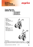
1
Robot Motion Robot Notes Robot Motion: Probabilistic Model; Sampling and Gaussian Implementations; Markov Localization September 2001 Kurt Konolige SRI International [email protected] http://www.ai.sri.com/~konolige 1 Robot Motion 1 2 3 4 5 6 Mobile Robots and Motion............................................................................................................. 4 1.1 Type of mobile bases.............................................................................................................. 4 1.2 Control and Controllability..................................................................................................... 4 1.2.1 Configuration Space ....................................................................................................... 5 1.2.2 Controllability................................................................................................................. 5 1.2.3 Control Regime............................................................................................................... 5 1.3 Dead-Reckoning ..................................................................................................................... 6 1.3.1 Position Estimation......................................................................................................... 6 1.3.2 Encoders and Precision................................................................................................... 7 1.3.3 Position Integration......................................................................................................... 7 1.4 Position Integration Errors ..................................................................................................... 9 1.4.1 Systematic vs. Random Errors........................................................................................ 9 1.4.2 Mobile Robot Random Errors ........................................................................................ 9 1.4.3 Error Representation for Position Integration................................................................. 9 1.4.4 Addition of errors ......................................................................................................... 11 1.4.5 Movement Error Units.................................................................................................. 12 1.4.6 Measuring Integration Errors........................................................................................ 12 Probabilistic Robot Error Model .................................................................................................. 14 2.1 Random Variables ................................................................................................................ 14 2.2 Robot Error and Motion as Random Variables .................................................................... 15 2.3 Robot Error Characteristics .................................................................................................. 17 Position Error Representation: Sampled Distributions................................................................. 18 3.1 Mean and Variance of a Sample Set..................................................................................... 18 3.2 Picking from a Sample Set ................................................................................................... 18 3.3 Robot Motion via Sampling ................................................................................................. 19 3.4 Extended Robot Motion ....................................................................................................... 20 3.5 Picking from a Distribution .................................................................................................. 21 Position Error Representation: Normal Distributions................................................................... 23 4.1.1 The Covariance Matrix ................................................................................................. 24 4.1.2 Rotation of Covariance ................................................................................................. 25 4.1.3 Initial Covariance ......................................................................................................... 26 4.2 Error Propagation under Exact Robot Motion...................................................................... 27 4.2.1 Error Covariance Units................................................................................................. 29 4.2.2 Error Evolution ............................................................................................................. 30 4.3 Total Error Updating ............................................................................................................ 30 Markov Localization using Sampling........................................................................................... 31 5.1 Markov Localization............................................................................................................. 31 5.2 Update using Samples .......................................................................................................... 31 5.3 Poisson Process .................................................................................................................... 32 5.4 Sonar Sensor Model ............................................................................................................. 33 5.4.1 On-Axis Sensor Model ................................................................................................. 33 5.4.2 Off-Axis Sensor Model ................................................................................................ 34 5.4.3 Mixtures and Gain ........................................................................................................ 35 Local Perceptual Space and Coordinate Systems ......................................................................... 36 6.1.1 Global Coordinate System............................................................................................ 36 6.1.2 Artifacts ........................................................................................................................ 37 6.1.3 The Robot Local Frame ................................................................................................ 38 6.1.4 Coordinate Transformations ......................................................................................... 39 2 Robot Motion 3 Robot Motion 1 Mobile Robots and Motion Mobile robots move in a large variety of ways. There are robots that walk, crawl, jump, swim, fly, and of course, roll. Some of these machines require very complex locomotion control, e.g., controlling helicopters or two-legged robots with dynamic balance is a very difficult control problem in its own right, and there are well-established research programs in both areas, as well as other forms of locomotion [refs]. But here we are more concerned with the challenges of navigation and localization, and we will look at only the simplest form of robot locomotion, namely a rolling robot that can turn and move forward or backward. 1.1 Type of mobile bases A mobile base must be capable of motion on a planar or near-planar surface, the ground plane. The simplest type of base has three degrees of freedom, its xy position and its orientation. More complex bases may have more degrees of freedom, e.g., articulated bases [ref Koren + Borenstein] may have two coupled parts. But most bases used for mobile robot research have a single body whose position and orientation can be controlled. Even within this framework, there are still a large variety of locomotion methods. 1. Ackerman drive. This is the typical car: steering front wheels, rear wheels for balance. 2. Differential Drive. In this method, two independently-driven wheels are placed on opposite sides of the robot. For balance, there is a passive caster wheel or wheels on the other sides of the robot. 3. Synchrodrive. This is a special type of base devised for indoor mobile robots. The Bxx series from RWI and the Nomad robots use this base. It has three driven wheels placed in a triangular pattern supporting the robot. The wheels all point in the same direction; when powered, the robot moves in that direction. Additionally, the wheels are connected by a belt drive to another motor that turns the wheels synchronously relative to the base. Hence, the robot can change its direction without rotating the base. 4. Omnidrive. This base is similar to the synchrodrive base, but each wheel is a complex mechanism that is capable of rolling in any direction. These bases make tradeoffs in design complexity, cost, performance, and ease of use. There are two performance criteria that are typically considered in mobile robot applications. • How easy is it to control the robot? Bases that allow the robot to turn in place, or to move in any desired direction without first turning, are much easier to control than ones that require extensive maneuvering to turn. We will look at the issue of controllability in Section XXX below. • How accurately can the base move? Typically bases have incremental encoders that keep track of wheel motion, and translate this motion into a dead-reckoned X-Y position. The accuracy of dead-reckoning is a critical factor in many mobile robot applications. Of course, this accuracy depends not only on the base, but also on the type of surface it travels on. In Section XXX we will discuss the types of dead-reckoning errors that occur, and comment on typical accuracies for various kinds of bases. 1.2 Control and Controllability How easy is it to move a mobile robot from one place to another? We’re all familiar with how hard or sometimes impossible it is to parallel-park a car in a space where it could fit. The difficulty lies in the nature or its steering: one cannot turn the car without moving it forward. In formal terms, the car has a nonholonomic constraint, that is, a constraint relating its position and velocity variables. Non-holonomic 4 Robot Motion constraints make it more difficult to control a vehicle, because it is not possible to move the vehicle in any desired direction. In this subsection we’ll look at these issues briefly, and also discuss the particular abstract control regime that a Saphira server must conform to. 1.2.1 Configuration Space Latombe, Robot Motion Planning [1991] Definitions, basic concepts. Question: which of the four base types have non-holonomic constraints? 1.2.2 Controllability Basic results on controllability: single non-holonomic constraints are still fully controllable. 1.2.3 Control Regime A base is controlled by applying power to its motors. Depending on the type of base, this will cause it move in a certain way. For bases of types 1, 3, and 4, the motors control the steering angle and forward motion. For differential drive, the motors control the motion of the two wheels: turning them both together makes the robot move forward or back, and moving them differentially causes the robot to turn (and perhaps also move forward or back). Both types of bases have two degrees of control, but they express it in different ways. From the point of view of controlling the robot’s motion, it’s easiest to think of the first Figure 1-1 Controlling the robot's velocity and type of control. It’s no accident that most of our angle vehicles (including planes and boats) are controlled by a steering wheel and an accelerator. You point in the direction you want to go, and you say how fast you want to go; furthermore, you can do this independently, that is, changing the steering angle doesn’t change the velocity. We’ll call this (v,φ) control. Figure 1-1 shows the idea: the robot’s instantaneous heading is given by φ (the direction of the arrow), and its velocity by v (the length of the arrow). By changing these variables, the robot executes the given trajectory. The robot is restricted to traveling smoothly, that is, the values (v,φ) change smoothly as the robot moves, depending on the power applied to the motors. To achieve a given velocity and heading, a feedback controller changes the motor power to move the velocity or heading to the desired value, and keep it there. The desired values are called setpoints. In typical digital controllers, the power value is recalculated hundreds of times a second, to achieve a tight tracking of the setpoints. Most bases provide such setpoints as part of their control electronics. 5 Robot Motion Velocity Position Translation speed(v) SfROBOT->setVel(int v) mm/sec move(d) SfROBOT->move(int d) mm Rotation rotate(v) SfRobot->(int ω) deg/sec turnto(φ) SfROBOT->setHeading(int φ) turn(φ) SfROBOT->setDeltaHeading(int φ) deg Table 1.1 Control channels and their setpoints Are there other reasonable choices for setpoints? Well, there are two control channels: rotation and translation. For each of these channels, we can choose to have either a velocity or position setpoint. (Why not acceleration?) For example, we could choose to move the robot a distance d and turn it to an angle φ. Or, we could choose to control the robots translational velocity v and rotational velocity ω. Table 1.1 shows the possibilities for each of the control channels. A particular control regime consists of one choice from each column. Saphira allows you to work in any control regime, and to switch control regimes at will, by calling the indicated functions. Note that the velocity and position control have very different effects on robot motion. Calling sfSetVelocity(100), for example, will start the robot moving until it attains a velocity of 100 mm/sec, and keeps it moving at that speed. On the other hand, calling sfSetPosition(100) will cause the robot to move forward 100 mm from its current position, and then stop. Rotational position has two functions: one for absolute angular position within the internal coordinate system, and one for relative position. sfSetDHeading(φ) moves the angular setpoint φ degrees from its current position. sfSetHeading(φ) moves the setpoint to the absolute position φ. In all of these functions, the maximum velocity achieved is set using the function sfSetMaxVelocity(int v). This sets the maximum velocity for each wheel. All of these control functions are interruptable, that is, issuing a new translational command interrupts the current robot translational motion by resetting the setpoint. It may also switch regimes, e.g., if the previous command was a positional one, and the new one is for velocity, then the translational control is switched from position to velocity. 1.3 1.3.1 Dead-Reckoning Position Estimation Almost all mobile robots use some kind of internal reference to keep track of their position as they move. Position estimation is useful for all kinds of task. On a very small scale, it can help to piece together individual sensor readings in a geometrically coherent manner, to give a better picture of the world around the robot. Such sensor fusion is especially important for robots whose sensors give them a limited view, e.g., those employing sonar or infrared proximity sensors. We’ll have much more to say about sensor fusion in Chapter XXX. Another important use for position estimation is navigation. Robots that must deliver goods from one place to another need to be able to tell when they have reached their goal, which areas they must avoid, and how to get from one place to another. One way to navigate is to keep track of their position in a map of their environment, and use that map to plan routes from one place to another. For example, hospital delivery robots like the one at Stanford have a precise floor plan of the hospital, and can navigate down corridors and through doors by keeping track of where it is in the plan. 6 Robot Motion There are many different ways to estimate position. Broadly speaking, we can divide these methods into two classes, internal and external. Internal methods rely on motion or forces produced by the robot itself, without regard to the external environment. External methods use some environmental signal to register the robot’s position. The signal can be a naturally-occurring one, such as the Earth’s magnetic field; or artificially created expressly for the purpose of position registration, as is the case with the Global Positioning System. Table 1.2 is a list of some of the better-known methods for position estimation, along Internal Methods Type Wheel Encoders Inertial Navigation Systems Precision mm cm Update Rate instantaneous 10 Hz Precision cm (differential) Update Rate 10 Hz cm mm 10 cm 1 degree 10 Hz 100 Hz 1 Hz 10 Hz External Methods Type Global Positioning System External Beacons Sonar Radio, Laser Landmarks Compass Table 1.2 Some Position Estimation Methods with typical precisions and update rates. Often several methods will be used together for more robust estimation, e.g., INS and GPS. In this case, the strengths of the systems are complementary: GPS gives reliable global position information, but tends to have high-frequency errors over the short term; the INS drifts with time, but gives a precise estimate for small local motions. Saphira relies on several methods to keep track of the robot’s position. Internally, wheel encoders give a precise estimate of the amount that the robot’s wheel have turned. More globally, a compass and the ability to locate sensed landmarks in a map keep the dead-reckoned position updated with respect to the environment. We’ll learn about the external methods in future chapters. 1.3.2 Encoders and Precision The robot’s position can be estimated by keeping track of how much its wheels turn. The principal mechanism for doing this is with incremental encoders, devices that are attached to a rotating shaft, and count as they are turned. A typical encoder might register 100 to 1000 counts for every revolution of the shaft. Most encoders also signal the direction the shaft is turning, by a method called quadrature encoding. The degree of precision of the encoders depends on their intrinsic counting ability, where they are mounted in the power train, and how large the wheels are. On most robots, it’s possible to achieve submillimeter precision when measuring wheel motion (see Exercise XXX). But precision is not the same as accuracy --- because of gear play, wheel slippage, and many other factors, the actual error of the robot’s position is estimated with significantly less accuracy. 1.3.3 Position Integration One of the most useful functions of internal sensors is to estimate the global position of the robot. Since internal sensors give information about the speed or distance the robot moves, and the change of angle of the robot, the information must be integrated to give its global position and direction. For 7 Robot Motion example, on Pioneer I the encoder counts are accumulated for 20 ms, and then used to perform motor control and to update the position of the robot. How do the encoder counts of the wheels relate to the ∆θ overall movement of the robot? Let’s assume we’ve figured out the relation between encoder counts and wheel distance, so that at the end of 20 ms the right wheel has moved a ∆r - ∆l distance ∆r , and the left ∆l . How far has the robot moved, and how much has it turned? ∆l If ∆r and ∆l are the same, then the robot has moved forward ∆r and hasn’t turned at all. If these two are different, then we can think of it in the following way (see Figure 1-2). Assume that ∆l is less than ∆r , and that d they’re both positive. Suppose both wheels moved forward Figure 1-2 Incremental motion of the ∆l at the same speed, keeping the robot straight, and then robot over a 20 ms period the left wheel stopped while the right one moved forward the distance ∆r - ∆l . How much did the robot turn? The turning motion happened at the end, as the axle of the robot rotated around the center of the left wheel, with the right end describing an arc of radius d (the length of the axle) and distance ∆r - ∆l . The angle ∆θ is simply the percentage of the circumference of the circle with radius d that the axle turned times the number of radians in a full circle, i.e., ( ∆r − ∆l ) 2πd × 2π radians, which is just (∆r − ∆l) d . How far did the center of the robot move? In the first part of the motion, it moved a distance ∆l . In the second part, the center of the robot moved ½ the ∆r − ∆l distance of the arc at the end, i.e., 0.5( ∆r − ∆l ) . ∆θ = Adding this to the original straight-line motion, we get d ∆r + ∆l 0.5(∆r + ∆l ) . Although we assumed that ∆r and ∆l ∆s = are both positive, the same analysis holds no matter what 2 their value. Equation 1.1 summarizes these results, the basic relationship between small wheel movements and Equation 1.1 Small wheel movements of a differential-drive base robot motion for a differential-drive base. The small robot motions can be integrated to give the global position of the robot. Figure 1-3 shows the path of the robot, broken into short segments that represent the information returned by the sensors. For Pioneer II robots, this occurs every 10 ms. Since the maximum speed of the robot is 2 m/s, the largest such segment is at most 2 cm in length. At any moment, the pose of the robot ∆s, ∆θ is given by the triple (x,y,θ) in the global coordinate system. If in the next time increment the robot moves a distance ∆s and turns ∆θ, then the new position of the robot ( x′, y ′,θ ′) can be calculated readily if we assume that the incremental motion is in a straight line. According to the analysis we just gave for the incremental x ′ = x + ∆s cos θ motion, we assume that the robot travels in y ′ = y + ∆s sin θ a straight line for the distance ∆s at the original angle θ, then turns an angle ∆θ. θ ′ = θ + ∆θ With this assumption, the updated Figure 1-3 Incremental position information integrated to give global position 8 Robot Motion coordinates are given by the simple functions shown in the figure. 1.4 1.4.1 Position Integration Errors Systematic vs. Random Errors Measurements taken with sensors are subject to many different sorts of errors. For example, a weight scale may consistently measure low because its spring is worn. Most sensors include some kind of calibration mechanism to correct for this systematic error, which arises from some mis-alignment in the sensor mechanism itself. In motion of differential drive robots, systematic errors can arise from many different sources. The main culprits are usually uneven or worn wheels, and errors in the distance between the wheels [ref Borenstein et al.]. All these problems introduce calibration errors into the chain from wheel motion on the floor to its measurement by the encoders and integration procedure. In the Pioneer robots, these calibration errors can lead to large errors in the integrated turn angle of the robot, and smaller errors in the estimated distance traveled. Because the turn angle is so important for position integration, there is a procedure for calibrating it. Note that the calibration can depend not only on the robot mechanics, but also on the environment. Different parts of the wheel will contact the ground on hard floors than on rugs, leading to differences in the actual axle length. In contrast to systematic errors, random errors are ones that cannot be calibrated out, either because they arise from unknown and/or unsensed interactions of the robot with the environment, or because they represent unmodeled behavior of the sensing chain. A typical example is wheel slippage, where the estimated distance the wheel travels is greater than the actual distance. 1.4.2 Mobile Robot Random Errors There are several sources of random error in position integration. These errors occur because of the finite width of the wheels (so the exact wheel contact can’t be predicted), deviations from roundness, wheel slippage, floor surface bumps, and other causes. Pile rugs are particularly bad: the pile nap can have an orientation that contacts the wheels on the inside or outside, depending on the direction of travel. Given that the robot may move a different amount at each wheel from the distance indicated by the wheel encoders, we can classify integration errors into three main types. • Range error. As the robot travels forward (or backwards), the integrated distance will differ from the true distance, as both wheels contribute to the error. This error grows with the distance traveled. • Turn error. Similar to range error, but for turns. As the robot turns, the integrated angle will differ from the true angle, as the difference of the wheel motions is in error. • Drift error. As the robot moves forward in a straight line, there may be a difference in the errors of the wheels, leading to a change in angle of the robot. [Figures would be nice here] Over long periods of time, turn and drift far outweigh range error, since they contribute to the overall position error in a nonlinear manner. Consider a robot whose position is initially perfectly well-known, and moves forward in a straight line along the x axis, according to the wheel encoders. Because of drift error, the robot’s actual angle will gradually differ from its true angle in the global coordinate system. The error in y position introduced by a move of d meters will have a component of d sin ∆θ , which can be quite large as the angular error ∆θ grows. 1.4.3 Error Representation for Position Integration How are position integration errors to be represented? It seems reasonable to represent range error, for example, as the average error in position over a standard distance, such as one meter. This average error is called the deviation. But what happens when the robot moves two meters? Is the deviation now 9 Robot Motion twice what it was for one meter? Intuitively, it should be less, at least if the errors are randomly distributed, since some of the error introduced in the first meter may be canceled by an opposite error in the second meter. To sharpen our intuitions, we’ll treat errors mathematically as random variables. Each random variable x represents a distribution of values; since we’re dealing with positions and angles, the variables are continuous, and the probability distribution is called a probability density function (PDF). A PDF is represented by a function p(x) over all values of x, where 0 ≤ p( x) ≤ 1 (1-1) ∫ p( x)dx = 1 An important concept in statistics is the expected value of a function of a random variable, defined as E ( f (x)) = ∫ f ( x) p( x)dx (1-2) The expected or average value of x is called the mean: ) x = E (x) (1-3) The distribution of values around the mean is called the variance, and is defined as: ) σ 2 = E ((x − x) 2 ) (1-4) From these definitions, one of the important properties of the sample mean is that: n ∑ (x n i − x) = i =0 ∑x i − nx = 0 (1-5) i =0 In statistics, we take samples from the population of a random variable x in order to determine these properties. Let xi be a set of n observations of the random variable x. The corresponding sample mean and sample variance are given by: n x= ∑x i i =0 n n 2 s = ∑ (x i − x) i =0 n −1 (1-6) n 2 = ∑ ∆x i 2 i =0 n −1 Note that the sample variance is defined using a divisor of n-1 rather than n. The sample data will be closer to the sample mean than to the true mean, and the smaller denominator compensates for this. In the limit of large n, the finite set will be a good approximation of this density function. The units of variance are the square of whatever the units of x are. The standard deviation is defined as the square root of the variance; its units are the same as x’s. The standard deviation is a good measure of the spread of the random variable x. If x is distributed as a gaussian function, then 68% of the area under the gaussian lies within a standard deviation of the mean; 95% is within two standard deviations. Thus, we should expect the value of x to be within a standard deviation of the mean 68 percent of the time. 10 Robot Motion 1.4.4 Addition of errors Now consider a robot that moves forward 2 meters, in 1 meter segments. Let x represent the motion of the first meter, and x′ the second meter (see Figure 1-4). What is the total variance in the robot’s position at the end of the move? […x′j…..] […xi…..] x$ ′ x$ […yij…..] y$ Figure 1-4 Robot motion in two steps. Each random variable x and x′ has a mean of 1 meter. The random variable y represents the total movement. To calculate the variance, consider the random variable y as composed of the addition of the 1-meter random variables, so that y ij = x i + x ′j . Then the variance of y can be shown to be: n var(y ) = n ∑ ∑ [( x i =0 j =0 i + x ′j ) − (xˆ + xˆ ′)] 2 n2 = var(x) + var(x ′) (1-7) The details of the reduction in (2.7) are left as an exercise. From this equation, we can answer the question just posed: the variance at the end of two meters is the sum of the variances from each of the 1meter moves. Thus, as is well-known from statistics, when two independent random variables with no constraints are added, the variances of the variables are added to produce the variance of the summed variable. The variance is the average of the squared error; the deviation is the square root of the variance. Assuming the errors in range are independent, the deviation in range after two meters will be 2 times the deviation after one meter. It’s important to keep in mind, though, that variances add for independent random variables. If there is systematic error in the position integration, then the situation can be worse. For example, suppose the wheels have worn down so their circumference is 90% of the assumed circumference. Then, in addition to small random variations in the integrated range, there will be a systematic underestimation of the range by 10%, and the range error will be dominated by it. Note that the systematic deviation is additive, rather than its variance. What all this means is that it’s important to try to identify systematic errors and correct them, so that the only errors are the independent random ones. For differential drive bases, and the Pioneers in particular, turning can introduce large systematic errors, depending on the type of surface the robot is on. If the surface is known beforehand, then it’s possible to correct for systematic errors by rotating the robot on the surface under controlled conditions. Another caveat is that the random variables must have no constraints for their variances to add. The derivation of (2.7) only holds if yij = xi + x′j ; this is true for position coordinates, but not for angles. In the case of angles, there is a singularity at 0 degrees, so yij = ( xi + x′j ) mod 360 . When computing angular differences ∆yij , the maximum angle difference is 180o, and thus ∆yij = ( ∆xi + ∆x′j ) mod 180 . For small angle differences, ∆yij will be close to zero, and the modulo addition won’t have much effect. For larger differences, however, it will; and in general, the total angular variance will be less than the sum of the two component variances. 11 Robot Motion 1.4.5 Movement Error Units Because of the additivity of variances, we’ll represent errors by their variance, that is, the average squared error. The following table summarizes the three types of errors. Error k R ∆s kθ ∆θ k D ∆s Units of kx mm2/m deg2/deg deg2/m Table 1.3 Position integration errors and their units If the robot moves forward a distance s, and turns an angle θ, then the variance will be: var(s) = k R s var(θ ) = kθ θ + k D s (1-8 ) NOTE: in this equation, s and θ are both positive values. θ is the amount of turning the robot does. 1.4.6 Measuring Integration Errors Measuring the range, turn, and drift errors of a robot can be tricky. For one thing, these errors will change depending on the surface the robot runs on: deep carpet, polished tile, grass. For another, it can be difficult to set up good experimental conditions for measuring the robot angle and distance traveled. In this section we’ll give some hints about how to measure the appropriate variables, as well as how to interpret the results of the measurements. Consider the case of measuring the range error. We’d like the robot to move a distance of, say, 1 meter, based on the encoder readings, and then we can check how far it actually moved. Using the Saphira client connected to the robot, we can move the robot forward using the joystick keys, and read the values of the encoder distance directly from the client window. But it’s difficult to stop the robot exactly at 1 meter; usually the best we can do is something like 990 or 1013 mm. Let’s look at a typical series of measurements: Encoder distance xe (mm) 890 1012 1003 Measured distance xm (mm) 930 1044 1020 Normalized measure xr (mm) 1045 1032 1017 The normalized measure xr is the measured distance xm normalized to an encoder count of 1 meter, that is, what we’d expect to measure at an encoder count of 1000 mm. This is easily derived as xr = xm ×1000 xe . Notice how the measured distances are always larger than the encoder estimation: the mean of the normalized measurements is 1031 mm, not 1000 mm. The difference between the mean x̂r and 1000 mm is the systematic error that we identified in the previous section. Systematic error, or error in the mean values of measured and estimated position, can be eliminated by simply recalculating the estimated value xe to be xˆ r 1000 of its original value. 12 Robot Motion Once the normalized measurements are calculated, then the random errors can be computed using the formula for the sample mean and variance (2-6). This is the average squared range error over a distance of one meter, which is the quantity we were interested in calculating. Turn and drift error can be calculated using similar techniques. In measuring turn and drift, it’s easiest to try to turn the robot so that it faces the same way it did at the start of the measurement, and then read off the angle change from the Saphira client window. 13 Robot Motion 2 Probabilistic Robot Error Model In this Section we take up the formulation of a probabilistic robot error model. The main elements of the model are a characterization of errors induced by motion of a differential-drive robot, and the addition of errors over a succession of moves. This general model will be the foundation, in subsequent Sections, for implementing several different forms of approximate models that are computationally tractable. 2.1 Random Variables We have already introduced the notion of random variables. Each random variable X represents a distribution of values; since we’re dealing with positions and angles, the variables are continuous, and the probability distribution is called a probability density function (PDF). A PDF is represented by a function f X ( x) over all values of X, where 0 ≤ f X ( x) ≤ 1 ∫f X ( x)dx = 1 (2-1) b P(a ≤ X ≤ b) = ∫ f X ( x)dx a The mean and the variance can be computed as before, via the expected values of x and the squared error. µ ≡ E ( X) = ∫ xf X ( x)dx σ 2 ≡ var(X) ≡ E (( X − µ ) 2 ) = ∫ ( x − µ ) 2 f X ( x)dx (2-2) The mean is the average value of the random variable. The squared error, also called the variance, represents the spread of the variable. Small variances mean the distribution is tightly peaked. There are two important types of random variables that we will use. The first is the normal distribution, whose PDF takes the shape of a Gaussian function. The definition is: N µ ,σ 2 ( x) ≡ 1 2π σ −( x−µ )2 e 2σ 2 (2-3) The normal distribution is symmetric around the mean, nonzero everywhere, and has most of its probability mass within 3σ of the mean. The variance of the distribution is σ . More generally, normal distributions have unique combination properties that we will exploit in this and following Sections. The Dirac delta function represents a probability mass concentrated at a single value of X. It is not a differentiable function, but has the following characteristics: 2 14 Robot Motion δ µ ( x) = 0, x ≠ µ ∫ δ µ ( x)dx = 1 ∫ f ( x)δ µ ( x)dx = (2-4) f (µ ) The variance of the delta function is 0. 2.2 Robot Error and Motion as Random Variables As before, we represent the robot’s current positional error using a 3-dimensional random variable, for x, y, and heading of the robot. For simplicity in the next few Sections, we’ll restrict the development to a scalar random variable X, the robot’s movement along the x axis. The question we want to address is: How does robot motion affect its uncertain position X? For example, suppose the robot moves a distance a along the x axis. How does X evolve under this motion? In general terms, we can represent robot motion as another random variable Y, with a parameter a that expresses the distance of the movement. Y(a) ≡ f Y ( a ) ( y ) Some examples: • No uncertainty. δ a ( y) . • (2-5) If the robot moves exactly a, then the movement random variable is Normal distribution of uncertainty. The movement random variable is a normal distribution centered on a. The variance of the normal distribution defines the uncertainty of the movement. Given an initial pose estimate X for the robot, and a movement variable Y, how do we calculate the robot pose estimate after the movement? The answer is given by the addition of the two variables: Z = X + Y(a) (2-6) Just as in the case of certain motion, we add the movement distance to the original pose of the robot. Since these are random variables, the addition also produces an updated uncertainty for the robot. To find this, we need to compute the value of Z, given the values of X and Y. The random variables are continuous distributions, not single values, so addition is more complicated than simple arithmetic addition. In fact, the addition of two random variables, represented by continuous PDFs, is not deterministic. To determine Z, we must consider the joint distribution X,Y. X, Y(a) ≡ f X ,Y ( a ) ( x, y ) (2-7) The random variable Z can be determined as the projection of the joint distribution down to a single distribution, for which x+y=z. f Z ( z) = ∫f X ,Y ( a ) ( x, y ) (2-8) z= x+ y 15 Robot Motion The integration over the set z = x+y can be accomplished by substituting the variable x = z-y (or y = z-x) in the integration: f Z ( z ) = ∫ f X ,Y ( a ) ( z − y, y )dy = ∫ f X ,Y ( a ) ( x, z − x)dx (2-9) It can be shown that, whatever the joint distribution X,Y, the mean of Z is just the sum of the means of X and Y. µZ = µX + µY (2-10) But, the same is not true of the variance of Z: in general, it will not be the sum of the variances of X and Y, but dependent on the exact shape of the joint distribution X,Y. What does the joint distribution look like? As we have said, it is not deterministic: there are many different joint distributions that will integrate to the marginal distributions X and Y. For example, consider X as the math test scores of a class, and Y as the verbal test scores. If there is a negative correlation between verbal and math ability, then the joint distribution X,Y will be skewed so that high math scores are often paired with low verbal scores, and vice versa. On the other hand, if Y is the physics scores of the class, then there will be a positive correlation, and high math scores will more likely be paired with high physics scores. If the random variables X and Y are independent (not correlated) then the joint distribution takes on a particularly simple form, the product of the two marginal distributions. The assumption of independence is also called the Markov robot motion assumption, because it has the same form as a probabilistic Markov chain. f X , Y ( a ) ( x, y ) = f X ( x ) f Y ( a ) ( y ) f Z ( z ) = ∫ f X ( z − y ) f Y ( a ) ( y )dy = ∫ f X ( x) f Y ( a ) ( z − x)dx (2-11) Under independence, the variance of Z is the sum of the variances of X and Y. var(Z) = var(X) + var(Y) (2-12) Note that this is the smallest variance that Z could assume. If the input variables are correlated, then the output variance will be larger. In systematic error, the deviation (square root of the variance) tends to add. For example, consider a robot that is mis-calibrated so that it always outputs a longer distance from the wheel encoders than the actual distance. If the error after moving 1 meter is 10 cm, then the error after moving 2 meters will be 20 cm. Some examples of particular distributions for X and Y: • Delta functions. The variance is zero for both X and Y, and the Z is a delta function with mean x+y. Note that for delta functions, the assumption of independence isn’t necessary. • Delta function and normal distribution. Let X be N a , s , and Y the delta function δ b . Then Z is the normal function N a +b , s . 16 Robot Motion • Normal distributions. Let X be N a , s , and Y be N b ,t . Then the independent joint distribution X+Y is just N a +b , s +t . Note that the variances of the input distributions are summed. 2.3 Robot Error Characteristics See Section 1.4. 17 Robot Motion 3 Position Error Representation: Sampled Distributions One method of approximating a PDF is to use discrete values of probability at selected points. A widespread representation of this sort are so-called occupancy grids [Moravec, Elfes], in which a geometric area is divided into a number of cells, and at each cell there is a probability of the cell being occupied by an object. Typically, probability grids of this sort are formulated using uniform grids, although other methods that conserve space are used, e.g., quadtree or octree representations [refs?]. The good thing about grids is that they can represent arbitrary PDFs, at least to some degree of precision based on the grid cell size. For example, it is easy to represent the robot being at one of two widely-separated locations. With analytic distributions, such as a normal distribution, this cannot be done (but mixtures of several normal functions are often used). An alternative to uniform grids is the notion of samples. A sample set can be considered as a nonuniform grid, where each sample represents the probability at some arbitrary point in the space. More formally, a sample set is a set of tuples, each tuple composed of a point and its corresponding probability. A sample set representing the random variable X has the following characteristics. s i ≡< xi , pi > P ( a ≤ X ≤ b) = ∑p a ≤ xi ≤ b ∑p i i (3-1) =1 A sample set with all probabilities equal is called a uniform sample set. For uniform sample sets, the density of samples is a measure of the value of the PDF. A set of samples represents one PDF exactly, namely, the one defined by Equation 3-1 above. By using enough samples, an arbitrary PDF can be approximated as closely as desired. But, it may take an exponential number of samples to do so. One nice property of sample sets is that the samples can be concentrated in the “interesting” part of the distribution, where most of the change in the distribution takes place. In this way, the variable parts of the distribution can be finely modeled, while the slowly-changing parts need few samples. 3.1 Mean and Variance of a Sample Set Instead of integration, we use summation. Interesting property: using only a random subset of the samples will give an approximation of the mean and variance. 3.2 Picking from a Sample Set An important operation is the notion of picking randomly from a sample set. “To pick randomly” means to choose an element based on its probability; elements with higher probability should be selected proportionally more times than those with a lower probability. For a uniform sample set, we choose uniformly from all elements. One of the applications for picking randomly from a sample set is to resample the sample set. In later Sections, we will use resampling to convert a sample set with non-uniform probabilities into a sample set approximating its PDF, but with uniform probabilities. A more immediate application is the combination of two sample sets into a joint distribution. Given the two sample sets X and Y, we want to form the joint sample set X,Y. As before, the joint distribution X,Y is underdetermined by the individual distributions X and Y. For example, let’s say that X are math scores for a class, and Y are verbal scores. Each student has a math and verbal score, and unfortunately 18 Robot Motion those students who do well in math tend to do poorly in verbal skills, and vice versa. In this case, the random variables are anti-correlated. If we form the joint sample set, we should more likely team up high values of X with low values of Y. A special case is when the individual variables are independent of each other. Now, if we choose any value of X, it will have no bearing on what we should choose from Y. A standard example is coin-tossing with a fair coin. Let X and Y will be uniform sample sets with approximately equal numbers of heads and tails. To form the joint distribution X,Y, we choose randomly from X, and then choose randomly from Y, using the two values to make up a new sample of the joint sample set. After proceeding in this way for a large number of samples, there should be approximately equal proportions of (h,t), (h,h), (t,h), and (t,t) tuples. [Change of variables] 3.3 Robot Motion via Sampling We return to the problem of adding two random variables, one representing the robot’s initial pose, the other the robot’s motion. Repeating Equation 2-6: Z = X + Y(a) ( 3-2) Here each random variable is represented by a sample set. How do we form Z? As before, we must consider the joint distribution X,Y, which is again a sample set, and construct Z by choosing members from X,Y and adding the x and y elements together. If we consider X and Y to be independent random variables, then we can form the joint sample set by picking independently from each of the single distributions. Now we have to consider the full three dimensional pose of the robot in constructing the updated pose set Z. The initial pose of the robot, X, is a uniform sample set with elements of the form < ( xi , y i ,θ i ), pi > ( 3-3) What about Y? First, for small robot motions, it is parameterized by the distance the robot moves, and the angle the robot turns: Y ( ∆s, ∆θ ) . The two parameters contribute to the three elements of the random variable Y: < ∆x, ∆y , ∆θ > . To pick a random element of Y, we start by picking elements from the random variables ∆s and ∆θ . We know these are normal distributions with mean ∆s and ∆θ , and variances given by: var(∆s) = k R ∆s var(∆θ ) = kθ ∆θ + k D ∆s (3-4 ) Section 3.5 discusses how to pick randomly from normal distributions. Once we have a sample from this set, we convert it into a sample of Y using the change of variables: ∆x j = ∆s j cosθ i ∆y j = ∆s j sin θ i (3-5 ) ∆θ j = ∆θ j 19 Robot Motion Here θi is the direction of robot motion, from the sample of X. Now we have all that is required to construct a sample of Z, which is: xi + ∆s j cosθ i y i + ∆s j sin θ i (3-6 ) θ i + ∆θ j The beauty of sample sets is that we can perform complex operations on PDFs, such as addition and change of variables, simply by picking samples correctly and performing the corresponding operations on individual values, rather than random variables. And, we don’t have to know anything about the form of the PDF. 3.4 Extended Robot Motion There is one further complication in applying Equation 3-6 to actual robot motion. This Equation is valid only in the case of small robot motion, where the robot moves in the direction of its original pose. Often we want to move the sample set representing the robot’s position only occasionally, after the robot has moved a significant distance. In this case, the direction of motion is not necessarily the same as the original direction; nor can it be found using the robot’s change of heading. Figure 3-1 shows the relevant geometry for an extended movement. The angle α is the difference between the original direction and the direction of motion. Note that it must be expressed as a local change in direction, since we will update samples with different headings for the robot. ∆θ p’= (x’,y’,θ’) ∆s α p = (x,y,θ) Figure 3-1 Geometry of extended robot motion. The direction in which the robot travels differs from its initial direction by an angle α. This angle is not necessarily the same as ∆θ. For extended motion, we could try to represent α as a random variable, but we won’t add this complication. α can be computed by looking at the poses p and p’ returned by position integration. The angle between the poses, minus the original heading θ, gives α. The method of computing Z from the previous Section remains unchanged, except for the final step. The updated values of the sample of Z are: xi + ∆s j cos(θ i + α ) y i + ∆s j sin(θ i + α ) (3-7 ) θ i + ∆θ j 20 Robot Motion NOTE: distance and total angle change (for variance) are approximations. 3.5 Picking from a Distribution In the sampling method, we are often confronted with the problem of picking from a particular distribution. Here we discuss a method for picking from a distribution, based on its cumulative distribution. Any time we can form the cumulative distribution, this method is applicable. For a random variable X with density function f X (x ) , the cumulative distribution is defined as P( X ≤ y ) , that is, the probability that the random variable is less than a value x. From the definition of probability density, we can write: y P( X ≤ y ) = ∫f X ( x)dx (3-8) −∞ We can use the cumulative distribution to define a picking strategy, based on uniform sampling. Suppose we pick some large number N of samples from X. First note that for any probability a, aN of the samples should have values taken from the beginning of the distribution f X (x ) up to the point where it integrates to the probability a. In terms of the cumulative distribution, aN of the samples should be less than or equal to x a , where P (X ≤ x a ) = a (3-9) How can we pick the set N? Suppose we start by picking from a uniform distribution in the interval [0,1]. Let the value picked be called a. Then, we find the x a that satisfies Equation 3-2, and use this value as a member of N. If we pick the entire set N in this way, it will satisfy Equation 3-2, in the limit of large N. For a standard normal distribution ( N 0,1 ), the cumulative distribution can be found using the error function. For any value x, the cumulative distribution is: PN 0 ,1 ( x) = 2) +1 erf ( x 2 (3-10) To find the value x a that satisfies a = PN 0 ,1 ( x a ) , we have to compute the inverse of the cumulative distribution. There are several ways to do this, the most common being some variant of Gauss-Newton iteration. For our purposes, a simple table-driven strategy will be good, because it can also be used for picking from discrete sample distributions. In the table method, we pre-compute a table of value of the cumulative function P. Generally, we will pick entries in the table based on where there are high values of the PDF underlying the cumulative distribution. For the standard normal function, values from –5 to 5 should suffice, since that is where most of the probability mass is distributed.. The table can be as fine-grained as required; a reasonable size is 100 entries. Given a value for a, which is between 0 and 1, the table is searched using recursive binary search. The middle entry is compared with a, and if it is higher, the search proceeds with the lower half of the table. If it is lower, the search continues with the upper half. Eventually two successive entries that 21 Robot Motion bracket a will be found, with indices i and i+1. An approximate value for the inverse function can be found by interpolating between the two entries, based on the value of a compared to the two entries. Applying the inverse cumulative function to a particular a will give a value z for the standard normal distribution. To convert this to an arbitrary normal distribution, use the change of variables: z = (x − µ ) σ x = σz + µ (3-11) 22 Robot Motion 4 Position Error Representation: Normal Distributions In the last subsection we saw how to measure and represent errors originating with the position integration mechanism of the robot. As the robot moves, these errors accumulate to make the robot’s overall position very uncertain with respect to its initial frame of reference. This uncertainty is produced by two mechanisms: • The addition of new position integration errors. • The evolution of previous errors under motion. To see how important this last contribution is, consider a robot located at the origin whose orientation is uncertain. Suppose this robot moves forward one meter with absolutely no error in range or angle: whatever its previous location was, it is at exactly the same orientation, just one meter forward (see Figure 4-1). Even though no new noise was added by position integration, still the robot’s position is more uncertain than it was initially, because we don’t know the direction in which it moved. It may have stopped at any of the positions along the arc depicted in Figure 4-1. The importance of angular uncertainty is evident from the figure. If you don’t know which way Robot initial position Robot final position 1 meter Angular uncertainty Figure 4-1 A robot’s uncertainty in position grows even when it moves with no dead-reckoning error, as long as it has an uncertain orientation. you’re heading, you don’t know where you’ll end up. Position error is very sensitive to angular uncertainty: even small orientation errors generate large position errors when traveling far enough. Ship navigation was only reliable after tools for determining the global heading of the ship were invented [some history would be nice here]. In the same way, accurate navigation for mobile robots in a global coordinate system means determining their orientation, and continuously correcting any angular uncertainty that may creep in. Location uncertainty (in the XY plane) is also important, but does not generate the large position errors that angular uncertainty does. Let’s change the previous example so that the robot heading is precisely known, but there is an initial location uncertainty. In this case, a precise movement of 1 meter does not change the uncertainty in location, although the mean position of the robot changes. So far we have been working with scalar random variables, whose statistics were defined by a mean value and a variance (average of squared error). In the case of a robot moving in a plane, there are three variables of concern: the position of the robot in the plane, and the orientation of the robot. These three variables are collectively known as the pose of the robot, and are typically represented by x, y, and θ. If these variables were independent, then their uncertainty could be represented by the variances var(x) , var(y ) , and var(θ ) . But this isn’t the case, as Figure 4-1 makes clear: the angular variance couples back to the robot’s position variance. 23 Robot Motion Let’s look at the coupling from another viewpoint. We’ve already said that the variances of independent random variables add. So, if all we’re interested in is the range and orientation errors of the robot, we can just look at how far the robot has gone, and how much it has turned, and compute the variances according to (2.6). The range and angle variances are independent, and just keep adding as the robot moves (with the exception that angle variance is limited). There is no interaction between the error in these variables. However, we need to know the position of the robot, not just how far it has gone. The robot’s position is dependent not only on the distance traveled, but also the instantaneous orientation of the robot. It is the coupling of orientation into the position variables that forces us to consider the robot’s motion in updating the pose variance. In this section we’ll lay the groundwork for determining how position error evolves with robot motion, by introducing the basic representational tool for error, the covariance matrix. 4.1.1 The Covariance Matrix We represent the pose of the robot by a column vector: Equation 4.2 x p = y θ p is a vector random variable with three components. It is important to note that this vector does not define a Euclidean space, since the third component is an angle. The first two components do define a Euclidean subspace of robot positions, and we’ll use the abbreviation q for this subspace. In the same way that the covariance for a scalar variable was defined (2.6), the covariance matrix for p is defined as the product of differences: Equation 4.3 n ∑ ∆xi ∆xi i =0 1 n 1 n T covar(p) = ∑ ∆p i ∆p i = ∑ ∆yi ∆xi n i =0 n i =0 n ∑ ∆θ i ∆xi i =0 n ∑ ∆xi ∆yi i =0 n ∑ ∆y ∆y i =0 n i i ∑ ∆θ ∆y i =0 i i n ∑ ∆x ∆θ i i ∆yi ∆θ i ∑ i =0 n ∆θ i ∆θ i ∑ i =0 i =0 n The diagonal elements of the covariance matrix are the variances of the elements of p. It is the offdiagonal elements that are new. Note that, because multiplication is commutative, the matrix is symmetric about the diagonal, so there are really only three new elements. To understand what they mean, it helps to consider cases where they are positive or negative. For example, let’s concentrate on just the x, y n subspace, and suppose that ∑ ∆x ∆y i =0 i i is positive. This means that, on average, whenever an x measurement is higher than the mean, the y measurement will be also. That is, the x and y values are positively correlated. If we draw a scatter plot of the x and y values, it will look something like this: 24 Robot Motion Figure 4-2 Skewed error ellipse for x and y positively correlated. If the off-diagonal elements are negative, then the ellipse will be skewed in the other direction, at a 45o angle counterclockwise from the y axis. If the off-diagonal elements are zero, then the ellipse axes align with the coordinate axes, and their magnitude is given by the variance of x and y. 4.1.2 Rotation of Covariance Often we will want to choose a different coordinate system for the variance. For example, in moving the robot, the variance from the position integration error will be given in the local coordinate system of the robot, that is, a coordinate system aligned with the robot’s orientation. To add this variance to the original position variance of the robot, which is in global coordinates, we need to transform it to the global coordinate system. Since variances are defined as differences, no translation is involved, and the transformation is just a rotation. How do vectors and covariance matrices transform under a coordinate system rotation? Consider the diagram of Figure 4-3, which shows a pose p, originally defined in the coordinate system [x,y], and its position in the rotated coordinate system [x’,y’]. y x’ p y’ α x Figure 4-3 A pose p in a rotated coordinate system The elements of the pose p in these coordinate systems are related by the following equations: Equation 4.4 x′ = x cos α + y sin α y′ = − x sin α + y cos α θ ′ = θ −α 25 Robot Motion For convenience, we can define a rotation matrix that will rotate a position: Equation 4.5 cos α R (α ) = − sin α 0 sin α cos α 0 0 0 1 One of the nice properties of rotation matrices is that the inverse and transpose are equal, and both are the same as the rotation matrix of the negated angle: Equation 4.6 R (α )T = R(α ) −1 = R(−α ) The rotation matrix doesn’t change the robot orientation, so the complete equation for the pose p’ in terms of p is: Equation 4.7 0 p′ = R (α ) p + 0 − α This last equation tells us how a particular pose transforms under rotation of a coordinate system. To transform a random pose p, we have to transform its mean (which is just a point) and its covariance. Remember that each of the elements that contribute to the covariance can be thought of as the outer product of two difference vectors, ∆p i and ∆p i transform, namely: Equation 4.8 T (Equation 4.3). We know how each of these vectors ∆p′i = R(α )∆p i T T T T ∆p′i = [R(α )∆p i ] = ∆p i R(α )T = ∆p i R(−α ) Note that because these equations work with differences from the mean, the extra angle addition of Equation 4.7 cancels out. Now the covariance matrix covar(p′) can be derived as: Equation 4.9 1 n 1 n T T ′ ′ ∆ ∆ = R(α )∆p i ∆p i R(−α ) p p ∑ i i n∑ n i =0 i =0 = R(α ) covar(p) R(−α ) covar(p′) = This derivation of the transformed covariance uses the technique of outer products on the difference vectors. An exercise asks for explicit confirmation of the steps involved in the equality chain. 4.1.3 Initial Covariance A simple application of the rotation transformation is to calculate the covariance matrix for a robot that starts out positioned exactly at the origin, facing at an angle θ (Figure 4-4). The robot makes a short move s in a straight line, and then turns an angle α counterclockwise. We have to assume the move is short, because the drift error over a longer distance would accumulate, and the robot would have more position and angle errors at the end. 26 Robot Motion Figure 4-4 A robot positioned at the origin and facing at angle θ moves forward s and turns α at the end. p is the robot’s final position. α s θ The robot covariance in the robot’s own coordinate system (at the beginning of the move) is given by the range, turn, and drift errors: 0 k R s 0 covar(p) = 0 0 0 0 0 kθ θ + k D s The global coordinate system is rotated by an angle − θ from the robot’s heading. Let p’ be the robot’s Equation 4.10 pose in the global system. Using the results of Equation 4.9, we know that: Equation 4.11 0 k R s 0 R(θ ) covar(p′) = R(−θ ) 0 0 0 0 0 kθ θ + k D s k R s cos 2 θ k R s sin θ cosθ 0 k R s sin 2 θ = k R s sin θ cosθ 0 k k s + 0 0 θ θ D Notice that the angular error was unchanged under rotation. However, the rotation does mix the x and y errors, resulting in skew along the global axes. If the robot’s initial orientation is along the global axes, then the off-diagonal terms are zero, and there is no skew. 4.2 Error Propagation under Exact Robot Motion We saw, in Figure 4-1, that position uncertainty can grow even when the robot’s movements are accurate. In this section we formulate the equations of evolution for the covariance matrix under exact robot motion. As in the previous section, assume that the robot moves a small distance s in a straight line, and then turns at the end an angle α. However, in this case the robot starts at an uncertain pose p, and makes an exact move --- no range, turn, or drift errors (Figure 4-5). 27 Robot Motion α s p’ p Figure 4-5 Exact robot motion from an uncertain position. The robot moves forward a short distance s, and at the end turns an angle α. The following facts hold for exact motion: • If the position p has no angular error, then the variance remains the same at p’: only the mean changes. • If there is angular error, then the x and y position errors will grow (in most cases; we’ll discuss exceptions below). • In all cases the angular variance ∆θ is unchanged by exact motion. We will prove these statements by formally deriving the change of variance under exact motion. To do so, we again resort to the construction of summation of points. In addition, because the equations of motion are not linear, we employ the method of Taylor expansion of a function. The function in question is a vector-valued one, that relates pi’ to pi and the motion parameters sand α. Referring to Figure 4-5, we can derive pi’ as: 2 Equation 4.12 pi′ = f ( pi , s,α ) where xi′ = f x ( pi , s,α ) = xi + s cosθ i yi′ = f y ( pi , s, α ) = yi + s sin θ i θ i′ = fθ ( pi , s,α ) = θ i + α Because these equations are nonlinear in θi, they are difficult to use in deriving expressions for the updated covariance matrix covar(p′) . Instead, we use the first two elements of the Taylor series expansion to get an approximate linear form. Equation 4.13 pi′ ≈ f (pˆ , s,α ) + F (pˆ )( pi − pˆ ) where F is the derivative of f. Because the pi are vectors, and the function f is vector-valued, the derivative of f is a matrix called the Jacobian of f. It typically arises in calculus when discussing change of variables in multi-variate functions. In this case, we are changing from the variables pi, s, and α to p’. Before defining the Jacobian, we note the following facts about the Taylor expansion: i.pˆ ′ ≈ f (pˆ ) ii.∆pi′ ≈ F (pˆ )∆pi The first one holds because all of the ∆pi sum to zero, leaving just first term. The second holds because ˆ ′ from the left side of Equation 4.13, and f (pˆ ) from the right. of the first, allowing us to subtract p Equation 4.14 28 Robot Motion The second fact is the one we need to derive the updated covariance, as we did in Equation 4.9. Instead of the rotation matrices, we use the Jacobian to transform the difference vectors. Equation 4.15 1 n 1 n T T ′ ′ ∆ p ∆ p = F (pˆ )∆p i ∆p i F (pˆ )T ∑ ∑ i i n i =0 n i =0 = F (pˆ ) covar(p) F (pˆ )T covar(p′) = Again, the equalities can be verified by working through the definitions of the point sums. What does the Jacobian F look like? Since we see ∆pi′ as a function of ∆pi , the relevant variables are x, y, and θ. The variables s and α are really parameters of the function f in this case. So, the Jacobian is written as: Equation 4.16 ∂f ( p ) ∂p pˆ ∂f x ∂f x ∂x ∂y ∂f y ∂f y = ∂x ∂y ∂f ∂fθ θ ∂x ∂y F (pˆ ) = ∂f x ∂θ ∂f y ∂θ ∂fθ ∂θ pˆ 1 0 − s sin θ = 0 1 s cosθ 0 0 1 By using the covariance transformation and this Jacobian, we can compute the updated covariance of p’. An easy way to do this is to note that the covariance matrix covar(p′) can be written symbolically as ∆p′∆p′T , and: Equation 4.17 ∆x − s∆θ sin θ ∆p′ = F (pˆ )∆p = ∆y + s∆θ cosθ ∆θ Using the outer product, we can find any of the elements of the covariance. For example, the upper left element is: Equation 4.18 ∆x′∆x′ = ∆x∆x − 2 s∆θ∆x sin θ + s 2 ∆θ∆θ sin 2 θ The influence of the angular uncertainty on position uncertainty is clearly seen. If ∆θ is zero, then there is no change in the uncertainty of x on an exact robot move. 4.2.1 Error Covariance Units It is important to keep in mind the units that are being used in the transformation. We have proposed mm for positions, and degrees for angles. For the covariances, we have mm2 and degrees2. These are useful units for displaying results. However, we have to be careful when mixing angular and positional differences, as in Equation 4.19. The second term on the right-hand side seems to have units of degreemm2, and the third term degree2-mm2. But we know these have to be in units of mm2. What’s going on? 29 Robot Motion The answer is that the term s∆θ should have units of mm. To see how this occurs, consider the small triangle below. The distance ∆x is computed as s sin( ∆θ ) . For small angles, this is approximately s∆θ , as long as the units of ∆θ are radians. So in calculating the terms of the updated covariance, be careful to convert the angular variances to radians. Alternatively, it might be more consistent to just represent angles by radians throughout. Figure 4-6 Incremental change in position. s ∆x ∆θ 4.2.2 Error Evolution Intuitively, it appears that errors should always increase as the robot moves, unless there is additional information (say, from sensors) that can correct them. But there are cases in which errors can decrease just from position integration. Consider a robot that starts out with zero position covariance, but a large angular one. The robot moves forward (exact motion) one meter. Its position variance is now high in a direction perpendicular to the move. The robot then turns around exactly 180o, and moves one meter back. If the moves were exact, it is at its starting position, and the positional covariance will again be zero. How does this scenario work out in terms of the covariance update equation? 4.3 Total Error Updating Finally, we can put together the influences of integration error and robot motion to give the evolution of the covariance for a small robot motion (s,α). Equation 4.19 covar(p′) = F (pˆ ) covar(p) F (pˆ )T + 0 k R s 0 R(θ ) 0 R (−θ ) 0 0 0 0 kθ α + k D s Here, the first term on the right-hand side represents the transformation of the initial pose error if the robot’s motion is exact. The second term is the additional error introduced by uncertainty in the position integration. 30 Robot Motion 5 Markov Localization using Sampling In this Section we develop the concept of Markov Localization, extending the ideas of Sections 2 and 3 to take into account sensor readings from the environment. 5.1 Markov Localization Previously we developed an uncertainty model for robot motion. Now we discuss how to extend this to several motion steps, where at each step we also use sensor information to localize the robot’s position. In general, under uncertain motion the error of the estimated robot position grows. Using sensor information and a map, it is possible to shrink that error estimate. Notation: let 0,1,2,… be a sequence of time steps. X n|m is the estimated position of the robot at time n, given sensor information up to and including time m. Using this notation, the estimated position of the robot from dead-reckoning is X n|0 , that is, no sensor information is utilized. In Markov Localization, progression from X n|n to X n +1|n +1 proceeds in two steps: X n +1|n ← X n|n [Prediction] (5-1) X n +1|n +1 ← X n +1|n [Update] The robot prediction/update process is Markovian if all information is encoded by the current pose of the robot. This means, for example, that the effect of sensor readings in the Update step is dependent only on the current position of the robot, not the past history of sensor readings. In terms of PDFs, the Prediction step is based on a motion model p ( x | x' , a ) , where x is the robot pose produced by an action a from the robot at x’. p n +1|n ( x) = ∫ p( x | x' , a) p n|n ( x' )dx [Prediction] (5-2) This Equation is exactly Equation 2-11, the addition of random variables for robot pose and robot motion. The Update step incorporates the sensor model, using Bayes’ rule to generate the posterior probability of a pose, given the sensor reading s. At each pose x, the probability of being at that pose is modulated by the probability of finding the sensor reading s from that pose: p n +1|n +1 ( x) = αp ( s | x) p n +1|n ( x) [Update] (5-3) The factor α is a normalization factor, to make the posterior distribution integrate to 1. 5.2 Update using Samples For a sampled distribution, the Update step of Equation 5-3 is readily implemented, by re-calculating the probability of each sample. The sensor model is p ( s | [ x, y,θ ]) , the probability of getting sensor reading s from the pose [ x, y ,θ ] . For each sample s i = [ xi , y i ,θ i ], p i , the probability is updated by: 31 Robot Motion pi′ = p( s | [ x, y,θ ]) pi [Update] (5-4) The updated sample set will now have non-uniform probabilities, and the probabilities will not be normalized (sum to 1). Normalization is easy to accomplish: just sum up the probabilities of the revised sample set, and divide each probability by the sum. Why should we want a uniform sample set? Because it will concentrate samples where there is the most probability mass. A uniform sample set Q’ can be constructed from a sample set Q by the following process: Do N times: (5-5) Pick a sample from Q based on its likelihood, and add it to Q’, changing its probability to 1/N. To pick a sample from Q based on its likelihood, we use the technique described in Section 3.5, to transform from a uniform random value on [0,1] to a random value on a distribution represented by its cumulative distribution. First, we form the cumulative distribution CQ of Q: x 0 , p0 x1 , p 0 + p1 (5-6) x 2 , p 0 + p1 + p 2 ... This is a cumulative distribution table. Given a value v on [0,1], we can use binary search to find the value of x for which the cumulative distribution is equal to v. Note that it is not possible to use interpolation on this table, since the sample poses are not ordered in any fashion. Because the resampling is done by picking from the original distribution based on likelihood, this technique is called importance resampling. 5.3 Poisson Process In formulating the sonar sensor model, we will need the concept of a Poisson process. Suppose we are looking at echoes from a number of targets in front of a sensor. Assume that echoes coming back from the targets have the following characteristics: 1. For any interval, the probability of getting an echo from some target is the same as that for any other equal, non-overlapping interval. 2. The mean number of echoes from an interval of size x is λx . A process with these characteristics is called a Poisson process. The probability that there will be no hits from an interval of size x is given by: P ( NHI > x) = e − λx (5-7) We are interested in the PDF for the random variable: there is some echo in the interval x. From the above formula, we can write the cumulative density function F(x) as: F ( x ) = 1 − e − λx (5-8) 32 Robot Motion The PDF is the derivative of the CDF: f ( x) = λe − λx (5-9) Equations 5-7 and 5-9 will be key ones in formulating the sonar sensor model. Typically, λ will be a random target detection rate, in target hits per meter, e.g., 5% chance of a hit in 1 meter. 5.4 Sonar Sensor Model The sonar sensor model is surprisingly complex. It must take into account the distance to the nearest target, the angle of the target to the sonar, and the noise characteristics of the sonar and its environment. Figure 5-1 shows the general setup of the modeling process. reading s ϕ d sensor target Figure 5-1 Sensor model geometry. The sensor is located a distance d from the nearest target wall. The wall is at an angle ϕ to the perpendicular. The sensor returns a reading s. The sensor model is p ( s | d , ϕ ) . We could construct it experimentally, by putting a sonar sensor into an environment with a target at a distance d and angle φ, and then estimating the probability model by observing the frequency of responses s. However, this would take a lot of sensor readings, and in general it would be biased by the characteristics of the environment. Instead, we will use a theoretic model of the sonar sensor and the environment, and calculate the sensor response. We will determine the sensor model in three steps: 1. On-axis sensor model (single reflection from target) 2. Off-axis sensor model (multi-reflections) 3. Gain reduction 5.4.1 On-Axis Sensor Model In this case, we assume the target is perpendicular to the sensor, i.e., φ=0. In Figure 5-2, the general form of the PDF is diagrammed. There is an initial region where random targets are detected, either from misfirings of the sonar sensor electronics, or from unmodeled dynamic objects or other unknown obstacles in the environment. Then, the true sensor return occurs with a maximum at s=d, in the form of a normal distribution. Finally, there is some chance that no sensor reading is returned, that is, neither a random nor the true target is detected. This gives a probability blip at the maximum sensor range m. Mathematically, the initial random target detection, up to the target distance d, is modeled as a Poisson process with rate λ F , the false positive rate. The true target reflection is assumed to be randomly distributed around its distance d. Further, the chance of being detected decreases with increasing distance, so the normal is attenuated by a (linear) factor β (d ) . After d and before m, the return is just from the true 33 Robot Motion p ( s | d , ϕ = 0) s→ Random target detection d m Out of sensor range True target detection Figure 5-2 General form of the sensor model for on-axis target returns. Target is at distance d, perpendicular to the sensor normal. target. In all cases, the true target return is further attenuated by the probability that a false target has already been detected. The total return is thus: s<d: λ F e − λ s + β (d ) N d ,σ F 2 sonar ( s ) P( NHI > s ) d ≤ s < m : β (d ) N d ,σ 2 ( s ) PF ( NHI > d ) sonar s = m: 5.4.2 d m 0 d (5-10) 1 − ∫ [ s < d ]ds − ∫ [d ≤ s < m]ds Off-Axis Sensor Model In this case, we assume the target is at a large angle to the sensor, i.e., |φ|>15. In Figure 5-3, the general form of the PDF is diagrammed. There is an initial region where random targets are detected, either from misfirings of the sonar sensor electronics, or from unmodeled dynamic objects or other unknown obstacles in the environment. Then, the true sensor return occurs starting at s=d. Instead of a normal distribution for a direct reflection, we have to model a multi-reflection, that is, the echo bouncing off several surfaces before returning. Finally, there is some chance that no sensor reading is returned, that is, neither a random nor the true target is detected. This gives a probability blip at the maximum sensor range m. Mathematically, the initial random target detection, up to the target distance d, is modeled as a Poisson process with rate λ F , the false positive rate. The multi-reflection return is also modeled as a Poisson process, with a different rate total PDF as follows: λR that will generally be greater than 34 λF . In this case, we get a Robot Motion s<d: λF e −λ Fs d ≤ s < m : λ R e −λR s ⋅ PF ( NHI > d ) s = m: 5.4.3 d m 0 d (5-11) 1 − ∫ [ s < d ]ds − ∫ [d ≤ s < m]ds Mixtures and Gain When the target is at an intermediate angle between 0 and 15 degrees, the PDF for the sensor model can be computed by interpolating appropriately between the on-axis and off-axis model for 0 ≤ x < m . As usual, the final probability for x=m is computed by subtracting the PDF up to m from 1. In practical applications, the theoretic sensor model must be modified because it will generally give results that are too certain. There are several reasons for this; the biggest ones are: 1. Sensor readings are not completely independent of each other, given robot pose. 2. The map can have errors. To moderate the effects of the sensor model, a uniform distribution can be mixed in. The uniform distribution is a no-information sensor model, which does not change the prior. p ( s | d , ϕ ≥ 15) s→ Random target detection d m Out of sensor range True target multi reflection Figure 5-3 General form of the sensor model for off-axis target returns. Target is at distance d, perpendicular to the sensor normal. 35 Robot Motion 6 Local Perceptual Space and Coordinate Systems Internal sensing and position integration can be used to maintain the robot’s position within a global coordinate system. Over time, this dead-reckoned position will have large errors, unless it is corrected by external sensing. Saphira maintains a structured set of coordinate systems within which the robot’s position is updated by dead-reckoning and external sensing. This system is called the Local Perceptual Space, or LPS. In addition to the robot position, other internal objects, called artifacts, are also represented in the LPS. These artifacts function as the internal models for objects in the real world, or for imaginary objects that help to define the robot’s world. In much the same way, maps are geometric representations of both real-world objects such as streets, and imaginary boundaries such as the equator or national boundaries. Included in the LPS are two Cartesian coordinate systems: a global system G and a robot-centric system R. The two coordinate systems are useful for different tasks. The robot-centric system, for example, is easier to use when avoiding obstacles, since the direction of an obstacle relative to the robot is readily extracted. The global system is better for navigation tasks using map information, since the location of landmarks can be fixed and used to update the global position of the robot. . The robot position in its own coordinate system never changes, but the position of artifacts will. Saphira handles the bookkeeping necessary to keep these two coordinate systems coordinated. 6.1.1 Global Coordinate System The global coordinate system G is a right-handed Cartesian system (see Figure XXX). Points in G are represented by vectors of three coordinates, the x, y position and an angle θ. That is, all points in G, like the robot, have an orientation as well as a position. More properly we should call points poses. Figure 6-1 Global coordinate system G and a pose (position and orientation) p. y axis pose p x axis The robot’s pose in G is the point R. When the robot first connects to Saphira, its pose is always [ ]T centered on the global origin, that is, R = 0,0,0 . As the robot moves, its position integrators give the approximate pose of the robot in G, and R is updated accordingly to be the mean of this pose. In one of the previous exercises, the covariance matrix for the robot was computed, and this formula can be used to update the robot’s uncertainty as it moves. Because we will be dealing with more than one coordinate system, we use the notation Cp to indicate the pose p in the coordinate system C. So, the robot’s initial position in G would be written as: Equation 6.20 G 0 R = 0 . 0 36 Robot Motion Even though the robot starts initially aligned with G, as it moves its position is updated by Saphira based on dead-reckoning. Since the dead-reckoning is inaccurate, eventually the robot’s internal idea of where it is in G diverges from where it actually is in the world. If the covariance matrix is calculated with the correct error parameters, then it will indicate the probability of finding the robot near its dead-reckoned position. In Saphira, the main window shows a portion of the LPS centered on the robot. This window uses the global coordinate system when the Local button is turned off in the Display menu. The robot appears as an icon of its approximate size, and an indication of its heading. As the robot moves, its icon’s position is updated in the LPS. Within the Saphira window, the x axis is aligned vertically from the bottom to the top, and the y axis points to the left. This is still a right-handed coordinate system, rotated 90 degrees counterclockwise. Angles are measured counterclockwise from the x axis. In Saphira, all positions are given in terms of millimeters, and all angles in terms of degrees. In most cases, the range of angles is the interval 0,360 ) , although there are also other intervals for special cases. The position of the robot in G is maintained in two places: the state reflection structure sfRobot, and the point artifact sfRobotOrigin (see the next section). In the sfRobot structure, the fields ax, ay, and ath refer to the global pose of the robot. [ 6.1.2 Artifacts Other objects can also be represented by poses in G. These poses, along with perhaps additional information, are called artifacts, because they exist in the internal geometric space of the robot. They may or may not correspond to objects in the real world. For example, Saphira always creates an artifact at the global origin. Figure 6-2 A corridor artifact. The center of the corridor is represented by a pose, whose orientation runs along the long axis of the corridor. The length and width of the corridor are parameters of the artifact. length width corridor c y axis x axis Some artifacts are meant to represent real objects. Typical here is the corridor artifact, which is defined by a pose, a width, and a length. Figure 6-2 shows a corridor artifact and its parameters. Note that there is no intrinsic direction to corridors, since they are symmetric under a 180 degree rotation. This symmetry can cause some confusion when trying to orient the robot with respect to the corridor, since the robot has the choice of going one way or the other. Most artifacts will be displayed in the LPS window, along with a label indicating their type Table 6-4 below gives the most common artifacts in Saphira, along with a list of their parameters. In the case where an artifact has an extent, such as corridors or doors, the pose point is at the center of the structure, and the 37 Robot Motion pose angle is oriented along the artifact length. More information is available from the Saphira user manuals. Table 6-4 Artifact types. type C structure parameters sfCORRIDOR sfLANE sfDOOR sfJUNCTION sfWALL sfPOINT corridor lane door junction wall point width, length width, length width width length − Several point artifacts are already defined by the Saphira system. sfGlobalOrigin is always situated at the origin of G, and is displayed as a circle. sfRobotOrigin is always at the pose of the robot, and does not display. 6.1.3 The Robot Local Frame Every pose p in the LPS has an associated orientation, and thus it defines its own local coordinate system. Of these, the most important is the robot pose R, which defines a coordinate system that is centered on the robot, and whose x axis points along the robot’s (Figure 6-3). Consider another point p located within the global coordinate system as shown. p also has coordinates in the robot’s frame of reference R. To distinguish which frame of reference we’re talking about, we’ll prepend the reference frame to the point. G Point p in the global frame p = x, y , θ Point p in the robot frame R p = x′, y′,θ ′ G p: x , y , θ R: x r , y r , θ r G Figure 6-3 The robot pose R in global coordinates defines a local coordinate system Any artifact in the LPS has both sets of coordinates in its data structure: if p is the variable name of the point, for example, then (p.ax, p.ay, p.ath) are the global coordinates, and (p.x, p.y, p.th) are the local coordinates. In Saphira, you can create artifacts with the functions 38 Robot Motion sfCreateLocalPoint/Artifact and sfCreateGlobalPoint/Artifact, depending on which coordinate system is more convenient. The corresponding coordinates in the other system are automatically added to the structure. As the robot moves, the position of the robot in the global space changes, and so does the position of an artifact in the robot-centric coordinate system. Saphira updates the robot-centric position of all artifacts that are on the pointlist. To put artifacts on the pointlist, use the function sfAddPoint. This function does not checks for duplicates, so you can add a point twice and have it updated incorrectly; use sfAddPointCheck if you’re unsure whether the point is already there. Are there cases where you won’t want a point in the pointlist? Yes — when the point is just an intermediate point in a geometrical calculation. At some point, you may decide to change the global position of a point. To do this, change the global coordinates in the point structure, and then use the function sfSetLocalCoords to update the robotcentric coordinates correctly. On the other hand, you may decide to change the local coordinates of a point; in this case, modify the local coordinates in the point structure, and then use the function sfSetGlobalCoords to position the point properly in the global space. A special case is when you want to change the global position of the robot. Suppose you do this by just changing the sfRobot.ax/ay/ath fields in the state reflector. That certainly will move the robot in the global system, and the robot’s local coordinates always stay fixed at zero. But all the artifacts will now have inconsistent local and global coordinates, since the robot has moved. The function sfMoveRobot takes care of this problem. There are other useful Saphira functions for moving artifacts; check the Saphira user manual. 6.1.4 Coordinate Transformations In many cases it’s useful to define points relative to the robot or to other artifacts in the LPS. The easiest way to do this type of construction is to make use of transformations between coordinate systems. Referring back to Figure 6-3, let’s try to calculate the position of the pose p in the robot frame R, represented by p = x′, y′,θ ′ . The easiest way to think of this is to imagine first translating the frame G so that its center coincides with the origin of R, then rotating it so that it aligns with R (what happens if these operations are performed in the reverse order?) From our previous work on rotating coordinate frames, we know that this works out to be: R Equation 6.21 R − xr G p = R (θ r ) p + − yr − θ r In a similar manner, the inverse transformation can be computed by first rotating the frame R to align with G, and then translating it to coincide with G. This yields: Equation 6.22 G xr p = R(−θ r ) p + yr θ r R Consider the diagram of Figure 6-3. If we know the coordinates of p2 and p3 in the system pR, then by transforming coordinate systems we can find the coordinates of p3 in p2. Or, if we know p3’s coordinates in p2, then we could transform them into pR’s system. Why is this an important idea? In future chapters, artifacts will be defined to represent objects sensed by the robot. For example, there may be a point artifact representing a person sensed by the robot, and we’d like to define a point 1 meter in front of the person as the place for the robot to go. In Figure 6-3, let 39 Robot Motion pR be the coordinate system of the robot, and p2 the person. The point p3 is 1 meter in front of p2, but this is in p2’s coordinate system. To define this point in the robot’s system directly is a complicated construction: figure out the angle of the line p2 - p3, then use trigonometric functions to calculate p3’s x and y coordinates. A much easier method is to define p3 indirectly by first defining it as a point in p2, then transforming it to pR’s system. We now introduce notation for transformation operations. As before, to distinguish the coordinate system in which a point is represented, we use a superscript, e.g., Rp3 is the point p3 represented in the frame of pR. Usually, we transform points into and out of the robot-centric system R, for example, between Rp3 and 2p3. Saphira defines two functions this purpose. sfChangeVP(a,b,c) takes a point b with local coordinates in R, and sets the local coordinates of c to be b’s position in the frame of a. Note that in this case, a is also defined as a point in R. So, sfChangeVP operates to change Rb into ab. In a similar manner, sfUnchangeVP transforms a point from another point’s coordinate system, into the coordinate system of the robot. In terms of the superscript notation, sfUnchangeVP operates to change a b into Rb. sfUnchangeVP(a,b,c) takes the point b defined in a’s coordinate system (again, a is defined as a point in R) and sets c’s coordinates to b’s position in R. For many motion operations of the robot directed at goal positions, this will be the most useful operation. P3 P2 PR Figure 6-4 Transforming Coordinate Systems 40