Download Tutorial on agent-based models in NetLogo

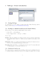
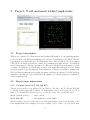
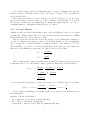
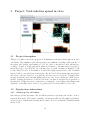
Tutorial on agent-based models in NetLogo
by Catherine Beauchemin ([email protected]) and Laura Liao
Department of Physics, Ryerson University
Last revision: June 11, 2012
Abstract
This tutorial will introduce the participant to designing and implementing an agentbased model using NetLogo through one of two different projects: modelling T cell
movement within a lymph node or modelling the progress of a viral infection through
an in vitro cell culture. Each project is broken into a series of incremental steps of
increasing complexity. Each step is described in detail and the code to type in is initially
provided. However, each project has room to grow in complexity and biological realism
so participants who finish more rapidly will be assisted in bringing their project beyond
the scope of the tutorial or in developing a project of their own.
Suggested reading
In preparation for the class and tutorial, participants are encouraged to read:
• N Moreira. In pixels and in health: Computer modeling pushes the threshold of medical
research. Science News, 169(3):40–44, 21 Jan, 2006
• C Beauchemin, J Samuel, J Tuszynski. A simple cellular automaton model for influenza
A viral infections. J. Theor. Biol., 232(2):223–234, 21 Jan, 2005.
doi:10.1016/j.jtbi.2004.08.001
• DM Catron, AA Itano, KA Pape, DL Mueller, and MK Jenkins. Visualizing the first
50 hr of the primary immune response to a soluble antigen. Immunity, 21(3):341–347,
Sep, 2004. doi:10.1016/j.immuni.2004.08.007
to understand how agent-based models of infection and/or immunity are typically made of.
1
1
NetLogo: A basic introduction
1.1
Getting NetLogo
To obtain NetLogo for your computer operating system (Mac, Linux, Windows), visit the
NetLogo website at http://ccl.northwestern.edu/netlogo.
1.2
Looking at a finished model from the Models Library
We’ll now have a look at what an example finished client looks like.
1. Select “File” → “Models Library”
2. Select “Sample Models” → “Biology” → “Tumor”
You see 3 tabs:
Interface: Where the simulation gets displayed and the end-user can interact with it using
the available sliders, buttons, etc. which were made available by the author of the
model.
Information: Where you can find general information about the model: what it is, how to
use it, etc. It is essentially the help page for the model.
Procedure: Where the NetLogo code driving the model is located. You can modify it and
see what happens or you can write brand new code.
1.2.1
Exploring the Interface tab
The “setup” button is a standard button in NetLogo and it is used to initialize the model,
i.e., set up the starting conditions for your model. For example, how many cells do you want
2
initially, where should they be, what colour should they be, what should be their initial state
(e.g., infected, uninfected, dead).
The “go” button does exactly what you’d expect: it makes the simulation go. But be
sure to press “setup” before you press go.
The remaining buttons allow you to trigger certain actions during the course of the
simulations. The various sliders and switches allow you to adjust various parameters or
conditions of the simulations: You can play around with them even as the simulation is
running. Finally, the monitors and plots are used to display variables of the simulations
(e.g., how many cells there are).
Note that if you want to restart the simulation, you can press “go” to stop the currently
running simulation and then press “setup” to reinitialize it.
Now that you know how to run a model, let’s learn how to make one.
1.3
Some NetLogo basics
The NetLogo User Manual is available at http://ccl.northwestern.edu/netlogo/docs/.
Here, I will provide a quick intro to help you get started.
A NetLogo simulation consists of a world made up of rectangles (in 2D) or blocks (in 3D)
called “patches” within which mobile agents called “turtles” can move and evolve based on
the turtles and patches around them and those encountered along their path. The patches
can also evolve; more on that later.
There are 3 types of agents of importance for us in NetLogo:
Patch: A small rectangle (in 2D) or block (in 3D) of the simulation world. A patch is
identified by its coordinate, (x, y) or (x, y, z). Thus it CANNOT move but it can hold
variables (e.g., its colour, how long ago it was visited, what type of a site it is). You
cannot have different breeds of patches: there is only one set of patches making up
your world.
Turtle: A mobile agent which can go from one patch to another based on whatever rules
are defined for its motion. Because it can move, a turtle agent is identified not by its
coordinate but instead by a “who” number. Turtles can also hold variables, and you
can have different breeds of turtles (different types of turtle agents, e.g., rabbits and
hares).
Link: A connection which can be created between two turtle agents. It appears as a line
corresponding to the shortest path between the two turtles. A link is identified by the
who number of the two turtles it links. Links can hold variables, and you can have
different breeds of links.
Note that by default the NetLogo world uses toroidal boundary conditions meaning that
anything which disappears off one edge of the world reappears on the opposite side. You
can change this (in NetLogo 2D only) under “Settings...” by unchecking the “World wraps”
checkboxes. For our two projects, we’ll use the default periodic boundary conditions.
3
1.4
Want to go further?
The projects below show you what to do step-by-step. But if you want to extend these
models or develop your own, the following resources will provide you with the information
you need:
NetLogo User Manual You will find it at http://ccl.northwestern.edu/netlogo/docs.
In particular, under Reference, check out the Programming Guide and the NetLogo
Dictionary (from the left-hand side menu).
Models Library You will find those within NetLogo under ‘File’ → ‘Models Library’. In
particular, check out the ‘Code Examples’ models which are very helpful. Most of these
codes are also available online at http://ccl.northwestern.edu/netlogo/models,
but not the ‘Code Examples’, unfortunately. Read the Models’ description to see if it
is likely to contain the type of code/behaviour you are looking to code-up in your own
simulation.
4
2
2.1
Project: T cell movement within lymph nodes
Project description
This project consists of T cells moving around within a 3D lymph node, encountering antigenloaded dendritic cells (DCs) and making brief contacts. You will first create 100 T cells and
have them move around randomly. You’ll then introduce 2 DCs and when a T cell encounters
a DC, the T cell will stop moving for 3 min before resuming its regular motion. You will keep
track of how many T cells have encountered a DC and you’ll plot how that number evolves
over time. You will also plot the tracks of some T cells, much like what gets recorded during
two-photon microscopy experiments. Some extensions of this project include: making each
DC bear different antigens and tracking how many cells have encountered each DC and how
many have encountered both, tracking how the number of contacts changes for different T
cell movement models.
2.2
2.2.1
Step-by-step instructions
Creating our set of T cells and DCs
This project is in 3D so you will need to use NetLogo 3D. Since our T cells and DCs will
be moving around, they will be turtles. To make things clearer, we’ll create two breeds of
turtles: T cells and DCs. At the very top of your ‘Procedure’ tab, you should enter:
breed [tcells tcell]
breed [DCs DC]
; the T cells
; the dendritic cells (DCs)
When creating a new breed, the first word is the plural name of the breed and the second
is its singular name. For example, if we were creating a breed of mice, we’d probably want
5
breed [mice mouse]. Note that ; is used to indicate a comment: everything after the ; is
ignored by NetLogo.
We’ll create the T cells and DCs as circles which map to spheres in NetLogo 3D. We’ll
make the DCs twice as large as the T cells. We’ll make 100 green T cells and 2 red DCs. So
let’s write the ‘setup’ function to do this:
to setup
clear-all
set-default-shape turtles "circle" ; all turtles will be circles (spheres)
create-tcells 100 [
set color green
; make T cell green
setxyz random-xcor random-ycor random-zcor ; put T cell at random location
]
create-DCs 2 [
set size 2
; make DC of size 2 (twice that of T cells)
set color red
; make DC red
setxyz random-xcor random-ycor random-zcor
]
end
Let’s link the ‘setup’ function to a ‘setup’ button. Go to your ‘Interface’ tab. Make
sure ‘Button’ is selected, press ‘Add’, and click anywhere in the Interface window. Under
‘Commands’ type ‘setup’, i.e. the name of the function you just created. Every time you
click the ‘setup’ button, your ‘setup’ function is run. Click it a few times to see how your
initial setup changes.
2.2.2
Setting the T cells in motion
We’d like to make our T cells move. To begin with, let’s make them move randomly, but with
a preference for continuing in their current direction (i.e. no drastic turn-arounds). We’ll
create a ‘go’ function just below our ‘setup’ function in our Procedure tab:
to go
ask tcells [
right random-normal 0 90 ; Pick random turn angle: avg = 0 std dev = 90 deg
roll-right random-normal 0 90 ; Pick random roll angle
forward 1
]
end
The ‘right angle’ command turns your turtle to the right by angle degrees. Here, instead
of specifying the exact angle, we use ‘random-normal 0 90’ which will pick a random angle
from a normal distribution of mean zero and standard deviation 90◦ .
6
Now, create a button as before, but this time enter ‘go’ in the ‘Command’ and check the
‘Forever’ checkbox. Click the button: wow, look at these T cells go! You can adjust the
speed with the slider.
But perhaps you’d like to create a button to see the T cells move by one step only.
Sure, create a button as before, enter ‘go’ in the ‘Command’, but this time, do not check
the ‘Forever’ checkbox and you might want to change the display name to ‘one step’ or
something similar to distinguish it from the other ‘go’ button.
2.2.3
Let’s get Physical
Alright, we have nice little balls moving around a grid, travelling at a speed of one patch
per time step. What is that?! We need to map the time and space in our model to REAL
physical time and space. Here is how to do this.
Since we did not specify the size of our tcells, NetLogo created them with a diameter of
one (1). So without even noticing, we have decided that a distance of 1 in our simulation
space corresponds to a physical distance of 8 µm in real life, i.e. the diameter of a T cell.
This seems like a good choice so we’ll leave it like that. As for time, let’s decide that each
time step of our simulation corresponds to 0.5 min (or 30 s). So let’s define
0.5 min
1 time step
8 µm
ds =
1 patch
dt =
Based on the two-photon microscopy literature, we know T cells move at a speed of about
16 µm/min. How do we convert that to units of patch per time step for use in NetLogo?
16 µm
0.5 min
1 patch
vNetLogo =
×
×
1 min
1 time step
8 µm
8 µm
1 patch
=
×
1 time step
8 µm
1 patch
=
1 time step
So, more generally, if you want to convert your real speed to a NetLogo speed, you’d write:
vNetLogo = vreal life ×
real time
1 patch
dt
×
= vreal life ×
1 time step real space
ds
So let’s adjust our simulation accordingly. At the top of our file, above all functions, add
the following line
globals [ dt ds tcell-step ]
; dt = duration of one step in min/time step
; ds = size of one patch in um/patch
; tcell-step = size of tcell step in patches/time step
7
in ‘to setup’ add
set dt 0.5 ; 0.5 min per time step
set ds 8
; 8 um per patch
set tcell-step 16 / ds * dt ; (16 um/min)*(1 patch/8 um)*(0.5 min/time step)
and modify your ‘to go’ to be
to go
ask tcells [
right random-normal 0 90
roll-right random-normal 0 90
forward tcell-step
]
tick-advance dt
end
Now your tick counter in the 3D View is in minutes. Let’s adjust its label accordingly.
Click on ‘Settings’ and under ‘Tick counter label’ enter ‘Time (min)’, and hit ‘Ok’. I also
recommend you set the update to ‘on ticks’ rather than ‘continuous’.
2.2.4
Designing T cell-DC contacts
Two-photon microscopy has taught us that when a T cell encounters a DC, it will pause
for about 3 min before resuming its regular motion. We also know that DCs have dendrites
approximately 19 µm [4]. Therefore, we can design T cell-DC contact by imposing the
following two rules:
• A T cell is considered in contact with a DC if it is within a radius of 19 µm of the DC.
Note that for us, this corresponds to a distance of 2 patches (19 µm × 1 patch/(8 µm)).
• A T cell stops moving for 3 min once it is in contact with a DC.
For this purpose it might make sense to use links. We will create a link between a T cell and
a DC when the distance requirement is met, and we could give the link a property tDCfree
which would keep track of the time left before the T cell is free from the DC.
At the top of the file, before the functions, add
links-own [ tDCfree ]
This states that all links will now have a variable called tDCfree. It is like globals
variables, but it belongs only to a specific type of agent, in this case the link agents. Next,
we’ll break the to go function into several functions to make the code clearer. In your code,
replace the to go function with
8
to go
move-tcells ; move T cell movement commands into a function
identify-DCbound-tcells ; new function to identify DC-bound T cells
update-link-status
; new function to update DC-T cell links
tick-advance dt
end
to move-tcells ; function for T cell motion
ask tcells [
right random-normal 0 90
roll-right random-normal 0 90
forward tcell-step
]
end
to identify-DCbound-tcells ; function to identify DC-bound T cells
end
to update-link-status ; function to update the DC-T cell links
end
Here, we’ve left the definition of the two new functions to later. It’s good to make your
changes incrementally. Now check that your code still works as before by pressing the ‘setup’
and ‘go’ buttons. If all is still working, you’re ready to start creating the identify-DCbound-tcells
function. What we want is to:
• Create a directed link from the DC and all T cells within a 2 patch diameter.
• Make the link red, just like the DC.
• Set the tDCfree to 3 min
• Make the linked T cells blue
Here is how you do this in NetLogo
to identify-DCbound-tcells ; function to identify DC-bound T cells
ask DCs [
create-links-to tcells with [ color != blue ] in-radius 2 [
set color red ; make the link red
set tDCfree 3 ; bound for 3 minutes
ask end2 [ set color blue ] ; make the linked T cell blue
]
]
end
9
For each DC, create-links-to creates a link from that DC to all T cells whose colour is not
blue which are located within a radius of 2 patches. The with [color != blue] ensures
that only T cells that are not blue (i.e. that are not already linked to a DC) are considered.
The ask end2 [...] means ask the turtle at the end of the link (in this case it is a T cell
since the directed link is from the DC to the T cell) to become blue.
That’s great, but now the T cells remain blue forever and their link to the DCs are never
removed. Time to write our update-link-status function:
to update-link-status ; function to update the DC-T cell links
ask links [
set tDCfree tDCfree - dt ; update time remaining for link
if tDCfree < 0 [ ; if tDCfree has elapsed
ask end2 [ set color green ] ; set T cell to its green colour
die ; kill the link (delete it)
]
]
end
Wow, this is awesome! But I sure wish we could track of how many encounters took place. . .
2.2.5
Counting the DC-T cell encounters
It would be nice to know how many DC-T cell encounters occurred. That’s where a Monitor
comes in handy. First, let’s create a global variable in our Procedure to keep track of DC-T
cell encounters: we’ll call it nDCmeet. So
globals [ dt ds tcell-step nDCmeet ]
; ...
; nDCmeet = number of DC-T cell encounters
and then somewhere within create-links-to in the identify-DCbound-tcells function,
you can add
set nDCmeet nDCmeet + 1
Now, in your ‘Interface’ tab, add a ‘Monitor’. Under ‘Reporter’ enter nDCmeet and under
‘Display name’ something like Number of DC-T cell encounters for clarity. Now run the
simulation and see how the Monitor gets updated and keeps growing as more and more
encounters occur.
2.2.6
Plotting the DC-T cell encounters
Ah, yes, a graph would be nice indeed. Here’s how you do this. In your to go function, just
above tick-advance dt add the following line
plotxy ticks nDCmeet
10
This will plot the number of DC-T cell contacts made thus far (nDCmeet) as a function of
time (ticks).
In your ‘Interface’ tab, add a ‘Plot’, call it something meaningful like Number of DC-T
cell encounters and set appropriate names for the x and y axis labels (e.g., time (min),
and Number). Now run the simulation and see what happens... cool!
2.3
Open-ended problems
Well, that was fun. Now it’s your turn! Below are a few challenging additions for you to
work into your code. If you have time, dive in and see how far you can get. Remember that
you can consult the NetLogo User Manual or the Models Library for additional information.
2.3.1
A 2-antigen system
This extension consists of making each of the 2 DCs bear different antigens and tracking how
many cells have encountered each DC, and how many have encountered both. You could,
for example, assign a different colour to your 2 DCs and have T cells change their colour to
match that of the DC they have encountered, and have each T cell record internally how
many times they have encountered each DC. You could also use colour to visually identify
those T cells which have encountered both.
2.3.2
The effect of T cell movement
This extension consists of exploring how different modes of movement for T cells affect the
number of DC-T cell encounters over the course of the simulation. For inspiration for T cell
movement, check out these references: [1, 3, 5].
2.3.3
Random walk versus chemotaxis
This extension consists of exploring the effect of chemokine-biased T cell movement. You
could make your DCs secrete chemokines (into their patch), have the chemokines diffuse
(check out the diffuse function) to neighbouring sites, and have T cells move preferentially
towards the sites with more chemokines (check out the uphill function).
11
3
3.1
Project: Viral infection spread in vitro
Project description
This project aims to model the progress of an influenza viral infection through an in vitro
cell culture. The simulation grid will represent your confluent cell culture with each site of
the square grid (patch) representing one cell. As cells become infected, they will undergo
a change of state (colour) going from uninfected (white) to latently infected (green) to
infectious (red) to dead (black). At each time step, you will determine if uninfected cells
become infected based on the number of infectious neighbours they have, and if latently
infected cells become infectious or infectious cells die based on how much time has elapsed
since these cells were infected. You will also add the action of cytotoxic T lymphocytes
moving around the grid randomly killing infectious cells. Some extensions of this project
include: plotting the fraction of cells in each state over time to monitor the progression of
the infection, adding the action of interferon or antivirals, or modelling extracellular virus
explicitly, or enabling cells to divide to repopulate the holes left behind by dead cells.
3.2
3.2.1
Step-by-step instructions
Setting up our cell culture
Since this project involves static cells, we will use patches to represent each cell and colour to
represent their state. We’ll want to initialize our infection with all cells uninfected (white),
except for a few of them in the latently infected state. For now, we’ll make 5 initially latently
infected cells.
12
In your ‘Procedure’ tab, you should enter
to setup
clear-all
; setup whole grid
ask patches [
set pcolor white ; uninfected
]
; setup initially infected cells
ask n-of 5 patches [
set pcolor green ; latently infected
]
end
Note that ‘;’ is used to indicate a comment: everything after the ‘;’ is ignored by NetLogo
so it allows you to leave yourself notes in the code to remember what the commands do. The
n-of 5 command tells NetLogo to pick 5 patches at random.
Now, let’s link the setup function to a ‘setup’ button. Go to your Interface tab. Make
sure ‘Button’ is selected, press ‘Add’, and click anywhere in the Interface window. Under
‘Commands’ enter setup, i.e. the name of the function you just created. Every time you
click the ‘setup’ button, your setup procedure is run. Click it a few times to see how your
initial setup changes.
3.2.2
Controlling the number of pfu in our inoculum
Instead of having 5 cells infected, we want to be able to set the number of cells to be initially
infected (i.e., the number of plaque forming units or pfu in the inoculum) directly from the
‘Interface’ tab. Let us call that number pfu.
First, add a ‘Slider’ to the ‘Interface’ tab, following the same procedure you used for
adding a button above, and enter the following information in the entry fields:
‘Global variable’
‘Minimum’
‘Maximum’
‘Value’
‘Units (optional)’
pfu
1
FIXME
5
pfu
leaving the rest of the fields as they were.
Second, replace the n-of 5 with n-of pfu in your ‘Procedure’ tab. Now if you go back
to your ‘Interface’ tab, you can try moving the slider to different pfu values and press ‘setup’
and verify that your slider successfully changes the number of initially infected cells. Ah,
look at you: now you control the initial inoculum. Such power!
13
3.2.3
Deciding who lives or die
Ok, so we have infected cells: now what? Well, these newly infected or eclipse cells, after
some time, will begin sythesizing viral proteins and soon they should be able to release virus,
becoming infectious. And after some time producing virus, these infectious cells will cease
viral production and undergo apoptosis either because they have exhausted the available
nutrients making all these virions, or due to toxicity resulting from viral production.
To reproduce this behaviour, we’ll have each cell keep track of when it should become
infectious and when it should die based on when it was infected. In your ‘Procedure’ tab,
above to setup, we will define the following patch properties:
patches-own [tinfectious tdead]
Now we have to make sure that, when we initially infect our pfu cells, all of them
decide right then when they should become infectious and die (i.e., set the value of their
tinfectious and tdead. So inside to setup, replace your ask n-of pfu section with this
one:
ask n-of pfu patches [
set pcolor green
set tinfectious 4
set tdead tinfectious + 7
]
so now our pfu infected cells have decided that they will become infectious after 4 ticks and
will die after 11 ticks (4 + 7). NetLogo uses ‘ticks’ to keep track of time.
Now we need to make time advance and keep track of whether these cells are ready to
change state. Below the end command marking the end of the setup procedure, add a new
go procedure.
to go
; check if latently infected cells become infectious
ask patches with [pcolor = green] [
if tinfectious <= ticks [
set pcolor red
]
]
; check if infectious cells die
ask patches with [pcolor = red] [
if tdead <= ticks [
set pcolor black
]
]
tick-advance 1 ; advance time by one time step
end
14
To run this procedure, create a button as before, but this time enter ‘go’ in the ‘Command’. Once the ‘go’ button has been created, click the ‘setup’ button and then the new
‘go’ button: the ‘ticks:’ number at the top of your simulation grid go up every time you click
on ‘go’ and when you get to ‘ticks: 5’, all your cells become red (infectious). If you keep
clicking, they’ll turn black (dead).
But all this clicking is not good for your wrist. It would be nice if it could just keep
going. Right-click on the ‘go’ button, select ‘Edit...’ and check the ‘Forever’ checkbox. Now,
if you click the ‘go’ button, it will go so fast that you won’t see a thing. You can adjust the
speed at which things happen by moving the slider at the top of the ‘Interface’ tab which
defaults to ‘normal speed’ but can be adjusted as you wish.
If you would like to keep the option of being able to make the simulation advance by just
one step, create another button with the command go, but do not check ‘Forever’ and set
the ‘Display name’ to something like ‘one step’ to distinguish it from the ‘go’ button. Now
you can ‘go’ continuously or one step at a time.
3.2.4
Making it big
It would be nice to look at a bigger patch of tissue. By default, NetLogo creates a grid that
is 33x33 where each square patch is 13 pixels wide. Here, we would prefer to have a higher
resolution image with more cells to look at.
In your ‘Interface’ tab, click on ‘Settings...’ and set:
max-pxcor 80
max-pycor 56
Patch size
6
Oh, much better. Click the setup and go button to see what things look like now.
3.2.5
Let’s get Physical
What we have now is patches which evolve as time in units of ticks goes by... we need to
connect time and space to real-life dimensions and units for our results to ultimately be
meaningful. Space-wise, let us say that one patch = one cell: that is simplest. Time-wise,
let us use units of hours. Now we need to reflect that choice in our procedures.
Each time step currently lasts 1 tick, and upon infection it will take your cells 4 ticks to
begin producing virus, and 11 ticks to die. In reality, for an influenza infection, the eclipse
phase, i.e. the pause between a cell’s successful infection by a virion and release of the first
infectious virion, takes ∼6 h [2]. An infectious cell will produce virus for ∼12 h before ceasing
viral production and undergoing apoptosis. Note that these times are approximate and vary
for different cell cultures, viral strains, and experimental conditions.
Let us define three global variable to help us keep time of the duration of a time step, the
eclipse phase, and the infectious phase. At the top of our ‘Procedures’, above patches-own
add the following lines
15
globals [
dt ; time step duration (h)
eclipsedur ; duration of eclipse phase (h)
infectiousdur ; duration of infectious phase (h)
]
It is always good to leave yourself comments about what your variables do and what units
they are in. We now need to set the value of these 3 variables. Inside to setup, right after
clear-all add
set dt 0.1
set eclipsedur 6.0
set infectiousdur 12.0
; 0.1h (6 min)
; 6h
; 12h
Still within setup, in the n-of pfu patches section, replace
set tinfectious 4
set tdead tinfectious + 7
with
set tinfectious eclipsedur
set tdead tinfectious + infectiousdur
To impose the duration of a time step, dt, in to go, replace the command tick-advance 1
with tick-advance dt. And to make these time-units obvious when looking at the simulation, go to your ‘Interface’ tab, click on ‘Settings...’ and under ‘Tick counter label’ enter
something like ‘time post-infection (h)’, and click ‘Ok’.
3.2.6
Spreading the joy... of infection
You might have noticed that right now your initially infected cells, though they become red
and are supposedly infectious, do not infect other cells. This is what we will fix now. We
could get complicated and allow cells to release virus and let virus diffuse outwards and infect
other cells... but that it a little too ambitious (see Section Open-ended problems below).
For now, let us assume infection is taking place under a thick agar so that infectious
cells can only infect their immediate neighbours. And let us assume that an infectious cell
can infect one of its uninfected neighbours every 6 min (that’s 0.1 h or one time step in our
simulation) until there are none left.
In ‘Procedures’, immediately after to go, add the following line
to go
spread-the-infection
and after the entire to go procedure, below end, add
16
to spread-the-infection
ask patches with [pcolor = red] [
let nnei count neighbors with [pcolor = white]
if nnei > 0 [ ; if more than 0 neighbours are uninfected
ask one-of neighbors with [pcolor = white] [ ; ask one of them
set pcolor green
set tinfectious ticks + random-normal eclipsedur (0.1 * eclipsedur)
set tdead tinfectious + random-normal infectiousdur (0.1 * infectiousdur)
]
]
]
end
The command let nnei count neighbors with [pcolor = white] will set variable nnei
equal to the number of uninfected neighbour the infectious cell has. And if it has more than
zero, it procedes to infect one of them.
The command random-normal eclipsedur (0.1 * eclipsedur) means that the duration of the eclipse phase for each newly infected cell will be chosen at random from a normal
distribution of mean eclipsedur and a standard deviation of 10% of eclipsedur. Having
these durations be random is more realistic because not all cells will become infected at the
same time. The same is true for tdead.
Time to test out your infection spread. Go back to ‘Interface’ and type ‘go’. Cool!
3.2.7
Sending in the death squad: adding cytotoxic T lymphocytes
This might not be entirely realistic for an in vitro cell culture, but it is a fun addition and
will allow you to see how to manipulate moving agents (turtles) since so far we have focused
exclusively on patches.
We will originally have 2 naive CD8+ T cells roaming the grid, moving randomly from
site-to-site. Upon encounter of an infectious cells, the naive CD8+ T cell becomes an effector
CTL. When an effector CTL encounters an infectious cell, it kills it. Effector CTLs divide
with a period of divtime to a maximum of maxdiv, after which it dies.
We will have to create a new breed of turtles: T cells. At the top of your ‘Procedures’
file, write
breed [tcells tcell]
tcells-own [ ttdead tdiv ndiv ]
and add the following variables to globals
globals [
divtime ; time between CTL division (h)
maxdiv ; max number of CTL divisions
In to setup you will need to add the following lines
17
set divtime 7.0
set maxdiv 7
set-default-shape turtles "face happy"
create-tcells 2 [
set size 2
set color magenta
setxy random-xcor random-ycor
]
which sets the time between T cells divisions to 7 h, and the number of divisions the CTL
will undergo before contraction to 7 division. Additionally, it specifies that the default shape
for T cells will be a happy face symbol. It then adds 2 magenta (naive) T cells at random
locations on the grid.
As for letting these cells move about, mature, divide and die, you will need to add the line
update-tcells just above tick-advance dt in to go, and at the bottom of the ‘Procedure’
file, add the following new procedure:
to update-tcells
ask tcells [
let pclr [pcolor] of patch-here
if (pclr = green) or (pclr = red) [
ifelse color = magenta [
set color cyan
set shape "face sad"
set tdiv ticks + random-normal divtime 1.0
set ndiv 0
][
ask patch-here [ set pcolor black ]
if tdiv <= ticks [
ask patch-here [
sprout-tcells 1 [
set shape "face sad"
set color cyan
set size 2
set tdiv [tdiv] of one-of other tcells-here
set ndiv [ndiv] of one-of other tcells-here
]
]
set tdiv ticks + random-normal divtime 1.0
set ndiv ndiv + 1
if ndiv > maxdiv [
die
]
]
18
]
]
right random 360
forward 1
]
end
3.3
Open-ended problems
Below are a few challenging additions for you to work into your code. If you have time, dive
in and see how far you can get. Remember that you can consult the NetLogo User Manual
or the Models Library for additional information.
3.3.1
Plotting the number of cells in each state
Using the command plotxy, you can plot the number of cells in each state over time. This
will allow you to monitor the progression of the infection, much like one could measure using
FACS (at least for infected cells).
3.3.2
Adding the action of antivirals
To simulate the action of antivirals, you could have a button in your ‘Interface’ tab which
turns the antiviral on at any time you wish. Its effect could be, for example, to lengthen the
time it takes for cells to begin producing virus (eclipsedur).
3.3.3
Implementing cell division
It would be nice if uninfected cells could divide to replenish the dead cells. For example, if
cells divide rapidly to regenerate dead cells, it might allow the infection to move back into
an area it had destroyed and this in turn could lead to chronic infection. A sensible rule
would be to give uninfected cells a probability to turn one of its dead (black) neighbour into
an uninfected (white) neighbour at every time step.
References
[1] J. B. Beltman, A. F. Marée, J. N. Lynch, M. J. Miller, and R. J. de Boer. Lymph node
topology dictates T cell migration behavior. J. Exp. Med., 204(4):771–780, 2007.
[2] B. P. Holder, P. Simon, L. E. Liao, Y. Abed, X. Bouhy, C. A. A. Beauchemin, and
G. Boivin. Assessing the in vitro fitness of an oseltamivir-resistant seasonal A/H1N1
influenza strain using a mathematical model. PLoS ONE, 6(3):e14767, 24 March 2011.
19
[3] T. R. Mempel, S. E. Henrickson, and U. H. von Adrian. T-cell priming by dendritic cells
in lymph nodes occurs in three distinct phases. Nature, 427(6970):154–159, 8 January
2004.
[4] M. J. Miller, A. S. Hejazi, S. H. Wei, M. D. Cahalan, and I. Parker. T cell repertoire
scanning is promoted by dynamic dendritic cell behavior and random T cell motility in
the lymph node. P. Natl. Acad. Sci. USA, 101(4):998–1003, 27 January 2004.
[5] M. J. Miller, S. H. Wei, I. Parker, and M. D. Cahalan. Two-photon imaging of lymphocyte
motility and antigen response in intact lymph node. Science, 296(5574):1869–1873, 7 June
2002.
20