Download Paper - STS

Project Work
Mathias Blumreiter
CTL Model Repair with NuSMV
October 4, 2015
supervised by:
Prof. Dr. Sibylle Schupp
Hamburg University of Technology (TUHH)
Technische Universität Hamburg-Harburg
Institute for Software Systems
21073 Hamburg
Eidesstattliche Erklärung
Ich versichere an Eides statt, dass ich die vorliegende Projektarbeit selbstständig verfasst
und keine anderen als die angegebenen Quellen und Hilfsmittel verwendet habe. Die
Arbeit wurde in dieser oder ähnlicher Form noch keiner Prüfungskommission vorgelegt.
Stelle, den 04. Oktober 2015
Mathias Blumreiter
Contents
Contents
1 Introduction
1
2 Fundamentals
2.1 Models . . . . . . . . . . . . . . . . . . . . . . . . . . . . . . . . . . . . . .
2.2 Properties . . . . . . . . . . . . . . . . . . . . . . . . . . . . . . . . . . . .
2.3 Binary and algebraic decision diagrams . . . . . . . . . . . . . . . . . . .
3
3
4
6
3 Model repair
9
3.1 Basic operations on models . . . . . . . . . . . . . . . . . . . . . . . . . . 9
3.2 Repairs and models with minimal change . . . . . . . . . . . . . . . . . . 10
3.3 Model update algorithm . . . . . . . . . . . . . . . . . . . . . . . . . . . . 12
4 BDD-based model checking with NuSMV
4.1 SMV models in the NuSMV input language . . . . . . . . . .
4.2 Processing of SMV models . . . . . . . . . . . . . . . . . . . .
4.2.1 Flattening of SMV models . . . . . . . . . . . . . . . .
4.2.2 Boolean encoding of variables and scalar propositions
4.2.3 Cone of influence reduction . . . . . . . . . . . . . . .
4.2.4 Model representation for unbounded model checking .
4.2.5 Model verification . . . . . . . . . . . . . . . . . . . .
4.3 Internal structure and programming paradigm . . . . . . . . .
.
.
.
.
.
.
.
.
.
.
.
.
.
.
.
.
.
.
.
.
.
.
.
.
.
.
.
.
.
.
.
.
.
.
.
.
.
.
.
.
.
.
.
.
.
.
.
.
.
.
.
.
.
.
.
.
16
16
18
19
20
23
23
24
25
5 Model repair in NuSMV
5.1 Integration into the SMV model processing procedure . . .
5.2 Basic assumptions and restrictions on SMV models . . . . .
5.3 Adapted basic operations on BDD-based models . . . . . .
5.3.1 Updating the transition relation . . . . . . . . . . .
5.3.2 Changing the label of a state . . . . . . . . . . . . .
5.3.3 Adding and removing of states . . . . . . . . . . . .
5.4 SMV model order, admissible and committed SMV models
.
.
.
.
.
.
.
.
.
.
.
.
.
.
.
.
.
.
.
.
.
.
.
.
.
.
.
.
.
.
.
.
.
.
.
.
.
.
.
.
.
.
.
.
.
.
.
.
.
.
.
.
.
.
.
.
27
27
29
30
30
31
32
34
6 Implementation
6.1 Limitations of the prototype . . . . . . . .
6.2 Integration into the NuSMV architecture
6.3 Repair procedure . . . . . . . . . . . . . .
6.4 Realisation of the update functions . . . .
.
.
.
.
.
.
.
.
.
.
.
.
.
.
.
.
.
.
.
.
.
.
.
.
.
.
.
.
.
.
.
.
36
36
37
38
40
.
.
.
.
.
.
.
.
.
.
.
.
.
.
.
.
.
.
.
.
.
.
.
.
.
.
.
.
.
.
.
.
.
.
.
.
.
.
.
.
7 Conclusion
44
8 Future work
45
iii
Contents
Bibliography
46
iv
List of Figures
List of Figures
2.1
2.2
2.3
BDD of f (x1 , x2 , x3 ) = ¬x3 ∨ (¬x1 ∧ x2 ) ∨ ((x2 ∨ ¬x3 ) ∧ (¬x2 ∧ x1 )) . . .
ROBDD of f (x1 , x2 , x3 ) with ord(x1 ) < ord(x2 ) < ord(x3 ) . . . . . . . . .
ROBDD of f (x1 , x2 , x3 ) with ord(x1 ) < ord(x3 ) < ord(x2 ) . . . . . . . . .
3.1
Given update functions by Zhang and Ding . . . . . . . . . . . . . . . . . 15
4.1
4.2
4.3
4.4
4.5
4.6
4.7
4.8
Model of a worker . . . . . . . . . . . . . . . . . . .
NuSMV processing procedure for BDD-based models
ROADD of counter : 0..4 . . . . . . . . . . . . . . .
BDD of ¬isEndReached . . . . . . . . . . . . . . . .
BDD of state and frozen variable mask . . . . . . . .
Masked BDD of ¬isEndReached . . . . . . . . . . .
Stored structure of property E[φ1 U (φ2 ∧ φ3 )] ∧ φ4 .
NuSMV package structure (architecture) . . . . . . .
.
.
.
.
.
.
.
.
.
.
.
.
.
.
.
.
.
.
.
.
.
.
.
.
.
.
.
.
.
.
.
.
.
.
.
.
.
.
.
.
.
.
.
.
.
.
.
.
.
.
.
.
.
.
.
.
.
.
.
.
.
.
.
.
17
19
21
22
22
22
24
26
5.1
5.2
5.3
5.4
5.5
Integration of the model repair into the processing procedure
Original encoding of status : {idle, wait, work} . . . . . . . .
Option 1 to encode tired . . . . . . . . . . . . . . . . . . . .
Option 2 to encode tired . . . . . . . . . . . . . . . . . . . . .
Application of P U 4 . . . . . . . . . . . . . . . . . . . . . . . .
.
.
.
.
.
.
.
.
.
.
.
.
.
.
.
.
.
.
.
.
.
.
.
.
.
.
.
.
.
.
.
.
.
.
.
28
32
32
32
33
6.1
6.2
6.3
Repair package . . . . . . . . . . . . . . . . . . . . . . . . . . . . . . . . . 37
Normal control flow . . . . . . . . . . . . . . . . . . . . . . . . . . . . . . 39
Needed control flow . . . . . . . . . . . . . . . . . . . . . . . . . . . . . . . 39
v
.
.
.
.
.
.
.
.
.
.
.
.
.
.
.
.
.
.
.
.
.
.
.
.
.
.
.
.
.
.
.
.
7
8
8
Listings
Listings
3.1
3.2
3.3
Model update: U pdateprop . . . . . . . . . . . . . . . . . . . . . . . . . . . 13
Model update: U pdate∧ . . . . . . . . . . . . . . . . . . . . . . . . . . . . 13
Model update: U pdateEU . . . . . . . . . . . . . . . . . . . . . . . . . . . 14
4.1
4.2
4.3
4.4
4.5
4.6
SMV model of a worker . . . . . . .
Binary counter . . . . . . . . . . . .
Binary counter (flattened) . . . . . .
Domain variables . . . . . . . . . . .
Representation variables (encoding)
Model of a resetable counter . . . . .
vi
.
.
.
.
.
.
.
.
.
.
.
.
.
.
.
.
.
.
.
.
.
.
.
.
.
.
.
.
.
.
.
.
.
.
.
.
.
.
.
.
.
.
.
.
.
.
.
.
.
.
.
.
.
.
.
.
.
.
.
.
.
.
.
.
.
.
.
.
.
.
.
.
.
.
.
.
.
.
.
.
.
.
.
.
.
.
.
.
.
.
.
.
.
.
.
.
.
.
.
.
.
.
.
.
.
.
.
.
.
.
.
.
.
.
.
.
.
.
.
.
.
.
.
.
.
.
17
19
19
20
20
21
List of Definitions
List of Definitions
1
2
3
4
5
6
7
8
9
10
11
12
13
Definition
Definition
Definition
Definition
Definition
Definition
Definition
Definition
Definition
Definition
Definition
Definition
Definition
(Kripke model) . . . . . . . . . . . . . . . . . . . . . . . . .
(Model) . . . . . . . . . . . . . . . . . . . . . . . . . . . . .
(Path, initial path, trace, and initial trace) . . . . . . . . .
(Reachable states, deadlock states, and deadlock) . . . . . .
(Computation tree logic (CTL) syntax) . . . . . . . . . . .
(De Morgan rules and equivalences for CTL properties) . .
(AEClass subset of CTL) . . . . . . . . . . . . . . . . . . .
(CTL semantic) . . . . . . . . . . . . . . . . . . . . . . . . .
(Valid model) . . . . . . . . . . . . . . . . . . . . . . . . . .
(Binary decision diagram (BDD)) . . . . . . . . . . . . . . .
(Ordered binary decision diagram (OBDD)) . . . . . . . . .
(Reduced ordered binary decision diagram (ROBDD)) . . .
((Reduced ordered) algebraic decision diagram ((RO)ADD))
.
.
.
.
.
.
.
.
.
.
.
.
.
.
.
.
.
.
.
.
.
.
.
.
.
.
3
3
3
4
4
4
5
5
6
6
7
8
8
14
15
16
17
18
19
20
Definition
Definition
Definition
Definition
Definition
Definition
Definition
(Model repair problem) . . . .
(Basic operation) . . . . . . . .
(Model update) . . . . . . . . .
(Model repair) . . . . . . . . .
(Partial order on Kripke models
(Admissible model) . . . . . . .
(Committed model) . . . . . .
.
.
.
.
.
.
.
.
.
.
.
.
.
.
9
9
10
10
11
11
12
21
22
23
Definition (Partial order on SMV models M0SMV ≤MSMV M00SMV ) . . . . . . 34
Definition (Admissible SMV model) . . . . . . . . . . . . . . . . . . . . . 35
Definition (Committed SMV model) . . . . . . . . . . . . . . . . . . . . . 35
vii
. . . . . . . .
. . . . . . . .
. . . . . . . .
. . . . . . . .
M 0 ≤M M 00 )
. . . . . . . .
. . . . . . . .
.
.
.
.
.
.
.
.
.
.
.
.
.
.
.
.
.
.
.
.
.
.
.
.
.
.
.
.
.
.
.
.
.
.
.
.
.
.
.
.
.
.
.
.
.
.
.
.
.
.
.
.
.
.
.
.
1 Introduction
1 Introduction
A challenge in the development of a complex system is to ensure that the implementation
satisfies the given requirements. Since development is inherently error-prone, many techniques have been devised over the years to check the resulting system for its correctness.
Model checking is one of the most widely used techniques. The reason is that model
checking is able to verify the system automatically without any interaction with the
system designer. Furthermore, the verified system does not need to be changed before
it is checked. The only prerequisite to do model checking is to represent the system and
its requirements in a way the model checker can work with. Hence, the system designer
has to provide an abstraction of the system in form of a model and an abstraction of its
requirements in form of properties that have to hold in the given model. The amount of
checkable requirements directly depends on the expressive power of the used property
language. There are a variety of property languages available. One popular property
language is the computation tree logic (CTL) which is supported by a large number
of model checkers. CTL is a branching-time logic that allows to express properties by
quantifying over the different execution paths in the model. A further advantage of
model checking is its ability to create counterexamples. Therefore, in the case that the
model checker can not verify a model for a given property, it generates a counterexample
to show where the property is violated. This enables the system designer to apply the
needed corrections to the model and therefore to the original system. Hence, model
checking does not only verify systems, but it also guides their repair by the generation
of counterexamples for the violated requirements. The model repair itself is an iterative
process of model verification and model update. The system designer has to repeat the
correction steps until all properties hold. Since the modifications are usually straightforward, it is apparent to automatise the entire repair process by exploiting the ability of
counterexample generation of model checkers. Hence, the aim of this project is to realise
an actual model repairer for CTL properties. However, although the required model
updates are usually straightforward for a single counterexample path, the validity of an
arbitrary CTL property depends on a number of execution paths as it quantifies over
them. It becomes even more complicated when a couple of CTL properties have to hold
at the same time. The reason is that the model updates for one property can directly
affect the validity of the other properties. Therefore, an approach is needed that takes
all this into account to perform the model repair in a systematic manner. This project
follows the model repair approach “CTL Model Update for System Modifications” by
Zhang and Ding [ZD10]. Furthermore, since the repair is guided by counterexamples,
a model checker is required to reason about the updated models and to generate the
needed counterexamples. Under the currently available ones, NuSMV is one of the most
well-known [Nusa]. The aim of the NuSMV project is to develop a robust state-of-the-art
model checker that can be used in technology transfer projects. Hence, NuSMV forms
the foundation of the implementation of the model repairer. Since NuSMV internally
performs the model checking in a way that is not covered by the approach of Zhang and
1
1 Introduction
Ding, this work focuses also on the transfer of their approach into the special situation
of model representation and model checking in NuSMV.
The work is structured as follows: chapter 2 gives an brief overview over the needed
basics regarding model checking. The model repair approach by Zhang and Ding is presented in chapter 3. Since NuSMV forms the basis for the implementation of the model
repairer, chapter 4 discusses the model checking procedure and the model representation
in NuSMV. The adaption of the model repair approach by Zhang and ding to the special
situation in NuSMV is described in chapter 5. Finally, chapter 6 discusses the current
prototypical implementation of the model repairer and chapter 7 summarises this project
and gives an outlook on future work.
2
2 Fundamentals
2 Fundamentals
This chapter gives a brief overview of the basics regarding model checking. If not stated
otherwise, the following definitions are given according to Logic in computer science modelling and reasoning about systems (2. ed.) by Huth and Ryan [HR04]. Hence,
please refer to this book for more in-depth information.
2.1 Models
The goal of model checking is to verify a system for its correctness. For that, a model
checker does not use the system directly, but an abstraction of it. The reason is that the
implementation details normally prevent an automatic verification. Since the properties
to be guaranteed are usually higher level requirements which are not affected by the
specific implementation details, the model only depicts the relevant parts that are useful
for an efficient verification. An example for such a situation is the verification of a
mutual exclusion protocol. Model checking can answer the question whether the protocol
satisfies the needed safety requirements. The verification of the details of the specific
implementation (i.e., the coding) is left to a more suitable verification technique. The
relevant parts of the system are given by a Kripke model.
Definition 1 (Kripke model).
Given a set of atomic propositions AP . The 3-tuple M = (S, R, L) over AP is called a
Kripke model whereby S is the finite set of states, R ⊆ S × S is the transition relation,
and L : S → P(AP ) is the labelling function.
Definition 2 (Model).
Given a Kripke model M defined over the set of atomic propositions AP . The 2-tuple
M = (M, S0 ) is called a model and S0 ⊆ S are called the initial states of M.
A Kripke model M is a 3-tuple of states, transitions and labelling function. Depending
on what is modelled, the states S can coincide with the real states the original system
can be in, or they can stand for something arbitrary. The system state change itself is
covered by the transition relation R. The labelling function L assigns to each state a
set of atomic propositions l ⊆ AP that hold at that state. They are used to define the
properties that have to hold for the entire model. But there is still a piece missing to
be able to check the properties. That are the initial states S0 as each system normally
starts in a well-defined state (or a couple of states). Hence, a Kripke model M together
with a set of initial states S0 forms what in the following is called a model.
Definition 3 (Path, initial path, trace, and initial trace).
Given a Kripke model M = (S, R, L) over the set of atomic propositions AP and a
model M = (M, S0 ) defined over M . Let S0 be an arbitrary non-empty set of initial
states S0 ⊆ S. A sequence of states π = [s1 , s2 , . . . ] is called a path in M respectively M if and only if all states in the path are also states in the (underlying) Kripke
3
2 Fundamentals
model si ∈ π ⇒ si ∈ S and for each two consecutive states in π exists a transition in
M connecting them si , si+1 ∈ π ⇒ (si , si+1 ) ∈ R ∀i ≥ 1. The infinite sequence of labels [L(s1 ), L(s2 ), . . . ] for π is called a trace in M respectively M. Furthermore, a path
π = [s1 , s2 , . . . ] in M starting at an initial state s1 ∈ S0 is called an initial path of M
and the corresponding trace an initial trace.
A path π in M is given by a typically infinite sequence of states [s1 , s2 , . . . ] which start
at an arbitrary state s1 ∈ S and where all consecutive pairs of states si , si+1 have
also a transition between them (si , si+1 ) ∈ R. The corresponding sequence of labels
[L(s1 ), L(s2 ), . . . ] is called a trace. It shows how the labelling changes when moving
along that path through the Kripke model. Hence, traces depict the behaviour of the
system. But as the system normally only starts in a couple of states and not all, only
certain traces depict the real behaviour of the system. Therefore, M represents the
behaviour of the modelled system by its set of initial traces.
Definition 4 (Reachable states, deadlock states, and deadlock).
Given a model M = (M, S0 ) with M = (S, R, L) as underlying Kripke model. A state
s ∈ S is called reachable if and only if there exists an initial path in M that contains s.
The set of all reachable states in M is represented by RS(M). A state s is called a
deadlock state in M if and only if it has no successor state (i.e., (s, s0 ) 6∈ R ∀s0 ∈ S).
Furthermore, the model M contains a deadlock if and only if a deadlock state is reachable.
2.2 Properties
The next step in the verification of the original system is to translate the requirements
into properties that have to hold in the model of the system. There are a variety of
property languages available. The expressive power of the respective chosen property
language directly affects the amount of requirements that can be verified. This work
only considers properties expressed in computation tree logic (CTL).
Definition 5 (Computation tree logic (CTL) syntax).
Given a set of atomic propositions AP . The syntax of CTL is defined inductively by:
φ ::= > | ⊥ | p ∈ AP | (¬φ) | (φ1 ∧ φ2 ) | (φ1 ∨ φ2 ) | (φ1 → φ2 ) |
EXφ | AXφ | EF φ | AF φ | EGφ | AGφ | E[φ1 U φ2 ] | A[φ1 U φ2 ]
Definition 6 (De Morgan rules and equivalences for CTL properties).
Let φ be a CTL property. The following equivalences hold for φ:
¬AF φ ≡ EG¬φ
AF φ ≡ A[>U φ]
¬EF φ ≡ AG¬φ
EF φ ≡ E[>U φ]
¬AXφ ≡ EX¬φ
A[φ1 U φ2 ] ≡ ¬(E[¬φ2 U (¬φ1 ∧ ¬φ2 )] ∨ EG¬φ2 )
4
2 Fundamentals
CTL is a branching-time logic that quantifies over the different execution paths in the
model. Furthermore, it also enables to reason about the future system change with
respect to the affected paths. For that reason, CTL supplements the syntax of boolean
formulas by introducing the temporal operators EX, AX, EF , AF , EG, AG, EU and
AU . The first letter refers to the quantification type: E for existentially quantification
and A for universally quantification. The second letter refers to the respective evolution
of the future (where the sub-property φ has to hold): X for next (= has to hold at the
next state), F for future (= has to hold at the current or a future state), G for globally
(= has to hold at all states from here on), and U for until (= φ1 has to hold from here
on until φ2 is satisfied).
Definition 7 (AEClass subset of CTL).
Given a set of atomic propositions AP . The syntax of the AEClass subset of CTL is
defined inductively by:
α ::= > | ⊥ | p ∈ AP | (¬α) | (α1 ∧ α2 ) | (α1 ∨ α2 ) | (α1 → α2 )
φ ::= α | EXα | AXα | EF α | AF α | EGα | AGα | E[α1 U α2 ] | A[α1 U α2 ] |
(φ1 ∧ φ2 ) | (φ1 ∨ φ2 )
An in the following important subset of CTL is AEClass (see Zhang and Ding [ZD10]).
AEClass contains the CTL properties without nested temporal operators. Hence, the
sub-property α of any temporal property φ can only be a propositional formula. Furthermore, negations are only allowed in the propositional part of the property. The semantic
of the AEClass properties follows the semantic of general CTL properties which is given
in the next definition:
Definition 8 (CTL semantic).
Let M = (S, R, L) be a Kripke model over the set of atomic propositions AP and φ be a
CTL property. Let s ∈ S be an arbitrary state of M . The satisfaction relation M, s φ
is given by structural induction on φ:
• M, s > and M, s 6 ⊥ ∀s ∈ S
• M, s p
iff p ∈ L(s)
• M, s ¬φ
iff M, s 6 φ
• M, s φ1 ∧ φ2
iff M, s φ1 and M, s φ2
• M, s φ1 ∨ φ2
iff M, s φ1 or M, s φ2
• M, s φ1 → φ2
iff M, s 6 φ1 or M, s φ2
• M, s EXφ
iff there exists a state s0 ∈ S with (s, s0 ) ∈ R so that M, s0 φ
• M, s AXφ
iff for all states s0 ∈ S with (s, s0 ) ∈ R: M, s0 φ
• M, s EF φ
iff there exists a path π = [s1 , s2 , . . . ] in M with s = s1 and a state
si ∈ π so that M, si φ
5
2 Fundamentals
• M, s AF φ
iff for all paths π = [s1 , s2 , . . . ] in M with s = s1 and for a state
si ∈ π: M, si φ
• M, s EGφ
iff there exists a path π = [s1 , s2 , . . . ] in M with s = s1 and for
all states si ∈ π: M, si φ
• M, s AGφ
iff for all paths π = [s1 , s2 , . . . ] in M with s = s1 and for all states
si ∈ π: M, si φ
• M, s E[φ1 U φ2 ] iff there exists a path π = [s1 , s2 , . . . ] in M with s = s1 and a state
si ∈ π so that M, si φ2 and M, sj φ1 for all j < i
• M, s A[φ1 U φ2 ] iff for all paths π = [s1 , s2 , . . . ] in M with s = s1 and a state
si ∈ π so that M, si φ2 and M, sj φ1 for all j < i
The difference between existentially and universally quantified properties is that there
has to be a path for existentially quantified properties whereas universally quantified
properties only require the validity of all existing paths. Hence, if there are none, then
universally quantified properties are satisfied. After the satisfaction relation for CT L
properties was given, the validity of models can be defined:
Definition 9 (Valid model).
Let M = (M, S0 ) be a model over the set of atomic propositions AP and P = {φ1 , . . . , φn }
be a set of properties. A property φ holds in the model M if and only if M, s0 φ holds
for all initial states s0 ∈ S0 of M (short M φ). Furthermore, a set of properties P
holds in M if and only if each individual property φi ∈ P holds in M (short M P ).
A model M is called valid with respect to P iff M satisfies all properties M P .
2.3 Binary and algebraic decision diagrams
A problem of model checking with explicit model representations (i.e., representing the
model as a graph) is the state space explosion problem. It prevents the verification of
large systems as the corresponding models become to large to fit into memory. McMillan
[McM93] proposed a solution to this problem by representing the model implicitly as
a set of boolean functions. Hence, the set of (initial) states, the transition relation
and the labelling function have to be expressed as boolean functions. Since the usage
of boolean functions alone does not allow to perform model checking, a suitable data
structure is needed to work with them. McMillan proposed the usage of ordered binary
decision diagrams. This is called symbolic model checking. However, since the specifics
of the general realisation of symbolic model checking are not important for this work,
this section concentrates on the definition of the decision diagrams. Please refer to Logic
in computer science - modelling and reasoning about systems (2. ed.) by Huth and
Ryan [HR04] or Symbolic model checking by McMillan [McM93] for an introduction to
symbolic model checking and the used operations of the decision diagrams.
Definition 10 (Binary decision diagram (BDD)).
Let f : Bn → B, (x1 , . . . , xn ) 7→ f (x1 , . . . , xn ) be a boolean function over n ∈ N0 boolean
6
2 Fundamentals
variables. A binary decision diagram (BDD) representing f is a finite directed acyclic
graph that is given by the following conditions:
• there is an unique initial node (the root node)
• all terminal nodes are labelled with T RU E or F ALSE
• each non-terminal node is labelled with a boolean variable xi
• each non-terminal node has exactly two outgoing edges to other nodes, the edges are
labelled with T RU E or F ALSE (depicted as solid and dotted lines), the labelling
of both edges differs
• the outgoing edges represent an assignment to the boolean variable of the node
• each path from the root node to a terminal node contains at most one non-terminal
node labelled with the boolean variable xi for all i = 1, . . . , n
• there is a path from the root node to a respective terminal node if and only if f
evaluates the assignments to the boolean variables on the path to the label of the
terminal node
An example of a binary decision diagram is depicted in Figure 2.1. The BDD represents
the boolean function f (x1 , x2 , x3 ) = ¬x3 ∨ (¬x1 ∧ x2 ) ∨ ((x2 ∨ ¬x3 ) ∧ (¬x2 ∧ x1 )). An
advantage of this representation is that the assignments for f (x1 , x2 , x3 ) = T RU E can be
directly read from the BDD. Furthermore, negating a BDD is considerably simpler than
negating other representations of the associated boolean function (e.g., the disjunctive
normal form). The only change to the BDD is the replacement of the labels of its
terminal nodes. The next step is to define a variable order for the BDD. This is needed
to make the BDDs for the two different boolean functions f (x1 , x2 , x3 ) and g(x1 , x2 , x3 )
compatible with each other. This enables the application of boolean operations between
these functions (e.g., conjunction, or disjunction) directly on their BDD representations.
x1
x2
x3
x3
T RU E
x3
F ALSE
T RU E
x2
T RU E
T RU E
x2
T RU E
F ALSE
F ALSE
Figure 2.1: BDD of f (x1 , x2 , x3 ) = ¬x3 ∨ (¬x1 ∧ x2 ) ∨ ((x2 ∨ ¬x3 ) ∧ (¬x2 ∧ x1 ))
Definition 11 (Ordered binary decision diagram (OBDD)).
Let f : Bn → B, (x1 , . . . , xn ) 7→ f (x1 , . . . , xn ) be a boolean function over n ∈ N0 boolean
variables. Let ord : {x1 , . . . , xn } → {1, . . . , n} be a bijective function depicting an arbitrary variable order for the n boolean variables. The BDD representing f is called
7
2 Fundamentals
ordered if and only if for any path connecting the root node to a terminal node the following holds: if a node labelled with xi occurs before a node labelled with xj in the path
(i.e., xi is closer to the root node), then ord(xi ) < ord(xj ) holds (with i, j ∈ {1, . . . , n}).
Since the aim is to check large models, the last step is to eliminate sub-graphs of the
OBDD that are redundant. This decreases the size of the OBDD significantly.
Definition 12 (Reduced ordered binary decision diagram (ROBDD)).
Let b be a OBDD. b is called reduced if and only if none of the following reduction rules
can be applied:
• isomorphic sub-graphs are merged
• non-terminal nodes whose children are isomorphic are removed
However, the size of resulting ROBDD directly depends on the chosen variable order for
the underlying OBDD. As an example, Figure 2.2 and Figure 2.3 depict two different
ROBDDs for the same BDD from Figure 2.1. The only difference is that the order of
x2 and x3 was swapped before the reduction. An advantage of the representation of a
boolean function as a ROBDD is that the ROBDD is a canonical representation of the
function with respect to a fixed variable order. Hence, different boolean functions can
be easily checked for their semantic equivalence by comparing their ROBDDs.
x1
x2
x1
x2
x3
T RU E
x3
x3
x3
x2
F ALSE
T RU E
Figure 2.2: ROBDD of f (x1 , x2 , x3 ) with
ord(x1 ) < ord(x2 ) < ord(x3 )
F ALSE
Figure 2.3: ROBDD of f (x1 , x2 , x3 ) with
ord(x1 ) < ord(x3 ) < ord(x2 )
Definition 13 ((Reduced ordered) algebraic decision diagram ((RO)ADD)).
Let (S, ◦, D) be an algebraic structure and f : Bn → S, (x1 , . . . , xn ) 7→ f (x1 , . . . , xn ) be
a function over n ∈ N0 boolean variables. The definition of algebraic decision diagrams
(ADD) follows the definition of binary decision diagrams (BDD) from Definition 10
except that the ADD for f is obtained by replacing the boolean terminal nodes with the
respective values from S. Furthermore, an ADD is already ordered and reduced according
to the definitions 11 and 12.
Algebraic decision diagrams are a generalisation of binary decision diagrams and were
introduced by Bahar et al. [Bah+93]. The main change is the extension of the codomain
of the represented function f to non-boolean values.
8
3 Model repair
3 Model repair
In contrast to other verification techniques, model checking is able to fully automatically check whether the properties hold in a given model. In case of an invalid model, a
counterexample is generated that shows where the property is violated. This helps the
system designer to modify the model and to transform it into a valid one. As the number of possible models is infinite and in general only a subset of them satisfy the given
properties, it can be quite challenging in practise to find a valid model. Furthermore,
for certain properties and models simple counterexamples alone do not provide enough
information to make systematic modification decisions. Buccafurri et al. [Buc+03] presented an example where no single counterexample path is a counterexample for the
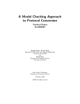
property AF AGa. This leads to the model repair problem.
Definition 14 (Model repair problem).
Let M = (M, S0 ) be a model over the set of atomic propositions AP and P = {φ1 , . . . , φn }
be a set of satisfiable properties with M, s 6 φ for a state s ∈ S0 and a property φ ∈ P .
The model repair problem is to transform M into a model M0 = (M 0 , S00 ) so that M0 P
holds.
It is assumed that the given properties are satisfiable, otherwise no repair would be
possible. The aim of model repair is now to automatise the modification process and to
perform the repair in a systematic manner. In the last years, different approaches have
been proposed. This project follows the model repair approach proposed by Zhang and
Ding. Hence, the following definitions are given according to “CTL Model Update for
System Modifications” by Zhang and Ding [ZD10].
3.1 Basic operations on models
Suppose there is a model that violates a given property. The next step in the repair
is to modify it in a way so that the property holds. As the model consists of a Kripke
model and a set of initial states, the modification is described by modifications on the
underlying Kripke model. Therefore, some operations on Kripke models are needed.
The following five basic operations are sufficient to compute any Kripke model out of a
given one.
Definition 15 (Basic operation).
Given a Kripke model M = (S, R, L) over the set of atomic propositions AP . An updated Kripke model M 0 = (S 0 , R0 , L0 ) is obtained by applying one of the following basic
operations:
PU1: Adding a new transition (si , sj ) 6∈ R between the two states si , sj ∈ S so that
S 0 = S, R0 = R ∪ {(si , sj )} =
6 R and L0 = L.
PU2: Removing an existing transition (si , sj ) ∈ R between the two states si , sj ∈ S so
that S 0 = S, R0 = R \ {(si , sj )} =
6 R and L0 = L.
9
3 Model repair
PU3: Changing the label of a state s ∈ S to l ⊆ AP so that S 0 = S, R0 = R, L0 (s0 ) =
L(s0 ) for all states s0 ∈ S 0 \ {s} and L0 (s) = l 6= L(s).
PU4: Adding a new state s with label l ⊆ AP so that S 0 = S ∪ {s} =
6 S, R0 = R,
L0 (s0 ) = L(s0 ) for all states s0 ∈ S 0 \ {s} and L0 (s) = l.
PU5: Removing an isolated state s ∈ S so that S 0 = S \ {s} 6= S, R0 = R and L0 (s0 ) =
L(s0 ) with neither (s, s∗ ) nor (s∗ , s) in R for all states s0 ∈ S 0 and s∗ ∈ S.
Definition 16 (Model update).
Let M = (M, S0 ) be a model with M as underlying Kripke model. The application of
a (sequence) of basic operation(s) on M is called a model update and M0 = (M 0 , S00 )
obtained by the updates on M is called the updated model.
Out of these five basic operations one is special. It is P U 3. One could argue that
P U 3 could also by implemented by a sequence of applications of the other four basic
operations. This claim is valid if one only looks at the structure of the graph and the
labelling function. As the model repair problem is essentially a search problem where the
starting point is the current model and a possible goal is a valid one, pruning conditions
have to be defined to reduce the available repair next steps. That is the reason for
the existence of basic operation P U 3. The availability of P U 3 allows to define more
restricting pruning conditions as the character of P U 3 does not match the character of a
sequence of applications of the other basic operations. The main difference is that P U 3
only changes the label of a state whereas the sequence (possibly) changes the (entire)
graph structure.
3.2 Repairs and models with minimal change
As stated before, the five basic operations are sufficient to compute any Kripke model,
but not every model update leads to a valid model with respect to the given properties.
Hence, it has to be distinguished between model updates and model repairs.
Definition 17 (Model repair).
Let M be a model and P a set of properties. A model update on M is called a model
repair if and only if for the obtained updated model M0 all given properties hold M0 P .
At his point, every model repair is a solution of the model repair problem. But from
the perspective of the system designer not every model repair is desirable. This results
from the fact that the model depicts the behaviour of the designed system. For example,
if a model is repaired with respect to universally quantified property then the easiest
repair is just to remove all transitions starting at the initial states. The updated model
is clearly a valid one, but no system behaviour is left. Other cases of undesirable repairs
are updates on models that keep the updated models valid but provide no advantageous
structure. This is, for example, the case when some unreachable substructures are
updated in a valid model. Therefore, an additional aim of model repair is to keep as
most of the system behaviour as possible and at the same time to change the model as
10
3 Model repair
little as possible. The minimal change condition implies that there is a way to measure
the change between the computed models. This is done by defining a partial order on
Kripke models.
Definition 18 (Partial order on Kripke models M 0 ≤M M 00 ).
Let M be the original Kripke model and M 0 , M 00 two Kripke models obtained by updates
on M . Let Dif fP U i (M, M 0 ) be the set of changes resulting from applications of basic
operation i on M (set of ... i = 1: added transitions, i = 2: removed transitions, i =
3: common states of both Kripke models with differing label, i = 4: new states, i = 5:
removed states). Furthermore, let dif f (L(s), L0 (s)) = (L(s) \ L0 (s)) ∪ (L0 (s) \ L(s)) be
the set of changed labels for the common state s ∈ S ∩ S 0 (i.e., the added and removed
labels). M 0 is called at least as close to M as M 00 (M 0 ≤M M 00 ) if and only if the
two following conditions hold:
1. for all sets of changes i = 1, ..., 5 : Dif fP U i (M, M 0 ) ⊆ Dif fP U i (M, M 00 )
2. if Dif fP U 3 (M, M 0 ) = Dif fP U 3 (M, M 00 ) then for each s ∈ Dif fP U 3 (M, M 0 ):
dif f (L(s), L0 (s)) ⊆ dif f (L(s), L00 (s))
The first condition is that all modifications performed on M 0 are also performed on M 00 .
The second one states that if the sets of common states with changed labels are equal
then the difference between the labelling of these states to the labelling in M has to be
contained in M 00 for M 0 . Thus, the labelling function for these states differs more to L
in M 00 but it contains the differences of M 0 , too. The principle of minimal change in
conjunction with the partial order gives now rise to the first pruning condition on the
repair search space.
Definition 19 (Admissible model).
Given the original model M = (M, S0 ), a model M0 = (M 0 , S00 ) obtained by updates on
M and a set of properties P . M0 is called admissible if and only if M0 P and there
exists no other model M00 resulting from updates on M with M00 P and M 00 ≤M M 0 .
The admissible model condition makes sure that the model is not changed needlessly.
If a model is already valid then it remains unchanged. At the same time it is clear
that admissible models are not unique. This results from defining this condition over a
partial order. So, if there are two alternative repairs for an invalid model where the first
one just removes a transition and the second one changes the label of a state then both
repaired models are admissible but the combination of both is not. As a consequence of
this condition, the repaired models only contain the minimal number of new valid paths
that are needed as any additional valid path violates the minimal change condition. This
is, for example, the case for the repair of M 6 φ1 ∨ φ2 where the model is only repaired
either with respect to sub-formula φ1 or sub-formula φ2 . Therefore, it can happen
that the model represents less behaviour than the system designer intended (e.g., only
M φ1 ∧ ¬φ2 ). This has to be taken into account when specifying the properties.
The admissible model condition prunes the search space drastically. But at this point
it is still likely to get repaired models that represent considerable less behaviour then
11
3 Model repair
the given one (i.e., in form of its initial traces, see Definition 3), since the behaviour
preservation was not taken into account up to now. This gives rise to the second pruning
condition.
Definition 20 (Committed model).
Given the original model M, a model M0 obtained by updates on M and a set of properties P . Let RS(M) ∩∼ RS(M0 ) = {s | s reachable in M and M0 ∧ L(s) = L0 (s)} be the
set of unchanged reachable states. M0 is called committed if and only if M0 is admissible
and there exists no other admissible model M00 resulting from updates on M where the
set of unchanged reachable states is larger RS(M) ∩∼ RS(M0 ) ⊂ RS(M) ∩∼ RS(M00 ).
In contrast to the first condition the committed model condition requires a number of
additional computation steps in each repair step. In order to meet the admissible model
condition, the repair algorithm just has to update the model in a way that the change is
minimal. So, if a valid model is found then immediately return. If the model is repaired
with respect to a (sub-)property, keep the (sub-)property valid. If a transition is added
then do no remove it later on, etc. In addition to that, the committed model condition
requires that in each repair step the next operation is chosen under the restriction that
the unchanged reachable states are maximal. As P U 1−P U 3 change either the transition
relation R or the labelling function L, they possibly change the unchanged reachable
states too. Now, if the algorithm wants to repair a model and P U 1 − P U 3 are applicable
to a couple of transitions/states then the algorithm would have to compute all updated
models and check their unchanged reachable states for maximality.
On the one hand, this approach preserves most of the system behaviour as possible, on
the other hand, the computational cost to compute committed models can become quite
high. Depending on the model representation, the check for maximality of two updated
models can be done in polynomial time. Zhang and Ding propose the method to compute
the reachable states by building a spanning tree of the underlying graph in polynomial
time. Furthermore, the maximality check has not to be done for all applications of
P U 1 − P U 3. If the label of a state was already changed then the next change does not
matter. If a transition to be removed does not disconnect a substructure or leads to
substructure only with relabelled states then this change also does not matter. But at
the end, all combinations of relevant updated models have to be taken into account.
3.3 Model update algorithm
This subsection presents three update functions to give an impression how the model
update algorithms work in principal. A couple of additional ones are depicted in “CTL
Model Update for System Modifications” [ZD10] (see Figure 3.1). It is important to note
that all update functions are designed to compute admissible models only. The impact
of updates on the unchanged reachable states is not considered. But as the majority of
these functions contain non-deterministic choices, one is free to chose the update that
preserves as most of the original model as possible. However, these choices are only
local whereas to be committed is a global characteristic of the model. Therefore, it can
12
3 Model repair
happen that early choices with few changes result in an heavily changed model at the
end.
Sometimes, the presented functions call the undefined method CT LU pdate. This is
just the entry point into the algorithm. CT LU pdate consists of a big case block that
identifies the type of the formula and then calls the respective update function (e.g.,
U pdateEU for E[φ1 U φ2 ] formulas, see Listing 3.3).
Listing 3.1: Model update: U pdateprop
Listing 3.2: Model update: U pdate∧
f u n c t i o n U pdate∧ ((M, s0 ), φ1 ∧ φ2 )
input
(M, s0 ) and φ1 ∧ φ2 , where
M = (S, R, L) , s0 ∈ S , and
(M, s0 ) 6 φ1 ∧ φ2 ;
output
(M 0 , s00 ) , where M 0 = (S 0 , R0 , L0 ) ,
s00 ∈ S 0 and (M 0 , s00 ) φ1 ∧ φ2 ;
begin
begin
a p p l y P U 3 t o change l a b e l i n g f u n c t i o n
i f φ1 ∧ φ2 i s a p r o p o s i t i o n a l formula ,
L on s t a t e s0 t o form a new model
then (M 0 , s00 ) = U pdateprop ((M, s0 ), φ1 ∧ φ2 ) ;
M 0 = (S 0 , R0 , L0 ) :
e l s e (M ∗ , s∗0 ) = CTLUpdate ( (M, s0 ) , φ1 ) ;
S 0 = S; R0 = R; ∀s ∈ S t h a t s 6= s0 , L0 (s) = L(s);
(M 0 , s00 ) = CTLUpdate ( (M ∗ , s∗0 ) , φ2 )
L0 (s0 ) i s d e f i n e d such t h a t L0 (s0 ) φ ,
with c o n s t r a i n t φ1 ;
and dif f (L0 (s0 ), L(s0 )) i s minimal ;
return (M 0 , s0 ) ;
return (M 0 , s00 ) ;
end
end
f u n c t i o n U pdateprop ((M, s0 ), φ)
input
(M, s0 ) and φ , where M = (S, R, L)
and s0 ∈ S ;
output
(M 0 , s00 ) , where M 0 = (S 0 , R0 , L0 ) ,
s00 ∈ S 0 and L0 (s00 ) φ ;
Source: “CTL Model Update for System Modifications” [ZD10]
Source: “CTL Model Update for System Modifications” [ZD10]
The simplest model repair is the satisfaction of a propositional formula (see Listing 3.1
for the associated update function). Since it is assumed that all given properties are satisfiable, there always exists a repair and the only admissible update choice is to change
the label of the given state s0 in a minimal way. This implies that L remains unchanged
if M already satisfies φ at s0 . Please note that the update functions are defined with
respect to a Kripke model and a single given state (which is normally not an initial
state). Hence, the Kripke model has to be repaired for each initial state one after another. Another option is to introduce a dummy state that has outgoing transitions to
all initial states and start the repair with this dummy state. The benefit is that the
repair algorithm can thereby add or remove initial states. As a drawback, all properties
have to be adapted obviously (add the temporal operator AX to each property), the
set of initial states is possibly changed (which may not be desirable in each case), and
the algorithm may chose this dummy state as a target of a new transition or consider it
when computing committed models. The next more difficult formula is a formula with
a boolean operator at the top level (¬, ∨, ∧). In case of negations, if it is a propositional
formula it is handled by U pdateprop . In all other cases, the De Morgan rules are applied
and CT LU pdate is called. Disjunctions φ = φ1 ∨ φ2 are handled as discussed before.
The algorithm chooses one sub-formula φi non-deterministically and continues the repair with it. The handling of conjunctions φ = φ1 ∧ φ2 is a bit different. The associated
update function is depicted in Listing 3.2. In contrast to disjunctions, the model has
to be valid for both sub-formulas. For that, the algorithm first repairs the given model
(M, s0 ) with respect to sub-formula φ1 and computes an intermediate model (M ∗ , s∗0 ).
Then it takes this intermediate model and repairs it with respect to sub-formula φ2
13
3 Model repair
which leads to the returned model (M 0 , s00 ). As (M 0 , s00 ) could be an invalid model for
φ1 , φ1 is a constraint for the repair of φ2 . This restricts the available repairs for φ2 to
those that also validate φ1 . As a consequence, there is always a set of constraints that
has be satisfied while repairing a model (which is not depicted in the update functions).
Listing 3.3: Model update: U pdateEU
f u n c t i o n U pdateEU ((M, s0 ), E[φ1 U φ2 ])
input
(M, s0 ) and E[φ1 U φ2 ] , where M = (S, R, L) , s0 ∈ S , and (M, s0 ) 6 E[φ1 U φ2 ] ;
output
(M 0 , s00 ) , where M 0 = (S 0 , R0 , L0 ) , s00 ∈ S 0 and (M 0 , s00 ) E[φ1 U φ2 ] ;
begin
i f (M, s0 ) 6 φ1 , then (M 0 , s00 ) = CTLUpdate ( (M, s0 ) , φ1 ) ;
e l s e do ( a ) o r ( b ) :
( a ) i f (M, s0 ) φ1 , and t h e r e i s a path π = [s∗ , ...] (s0 6= s∗ )
such t h a t (M, s∗ ) E[φ1 U φ2 ] ,
then a p p l y PU1 t o form a new model M 0 = (S 0 , R0 , L0 ) :
S 0 = S; R0 = R ∪ {(s0 , s∗ )}; ∀s ∈ S L0 (s) = L(s) ;
( b ) s e l e c t a path π = [s0 , ..., si , ..., sj , ...] ;
i f ∀s s0 < s < si , (M, s) φ1 , (M, sj ) φ2 ,
but ∀s0 si+1 < s0 < sj−1 , (M, s0 ) 6 φ1 ∨ φ2
then a p p l y PU1 t o form a new model M 0 = (S 0 , R0 , L0 ) :
S 0 = S; R0 = R ∪ {(si , sj )}; ∀s ∈ S , L0 (s) = L(s) ;
i f ∀s s < si , (M, s) φ1 , and ∀s0 s0 > si+1 , (M, s0 ) 6 φ1 ∨ φ2 ,
then a p p l y PU4 t o form a new model M 0 = (S 0 , R0 , L0 ) :
S 0 = S ∪ {s∗ }; R0 = R ∪ {(si−1 , s∗ ), (s∗ , si )} ;
∀s ∈ S , L0 (s) = L(s) , L(s∗ ) i s d e f i n e d such t h a t (M 0 , s∗ ) φ2 ;
i f (M 0 , s00 ) E[φ1 U φ2 ] , then return (M 0 , s00 ) ;
e l s e U pdateEU ((M 0 , s00 ), E[φ1 U φ2 ]) ;
end
Source: “CTL Model Update for System Modifications” [ZD10]
The last type of formulas are the ones with a temporal operator at the top level. An
exemplary update function is depicted in Listing 3.3. This is the one for the temporal
operator EU . The main difference between the previously presented update functions
and the ones for temporal operators is the reasoning about paths in the Kripke model.
This can be seen in the first else branch in Listing 3.3. U pdateEU tries to transform an
invalid path into a valid one to form an admissible model for the formula E[φ1 U φ2 ]. For
that, it chooses one of two repair strategies non-deterministically. The first strategy is
to connect the given state s0 to a state s∗ in the Kripke model where M, s∗ E[φ1 U φ2 ]
already holds. The second strategy is to take a path starting at s0 where φ1 holds in
the beginning up to a state si and where φ2 holds later at sj . The algorithm then adds
the transition (si , sj ) to R to jump over the states where neither φ1 nor φ2 hold. In
the case that no such state sj exists, U pdateEU introduces a new state s∗ with a label
that satisfies φ2 . s∗ is then inserted into the path between si−1 and si . As φ1 holds up
to si or si−1 and φ2 holds at sj or s∗ , M, s0 E[φ1 U φ2 ] should hold, too. If that is
not the case then U pdateEU tries to repair the current updated model (again). Since in
each repair step the number of available paths to choose from decreases, U pdateEU will
terminate eventually.
14
3 Model repair
Property type
Repair realised by update function
Propositional formula U pdateprop
φ1 ∧ φ2
U pdate∧
φ1 ∨ φ2
U pdate∨
¬φ
U pdate¬
EXφ
U pdateEX
AF φ
U pdateAF
E[φ1 U φ2 ]
U pdateEU
AXφ
by equivalence with EX
EF φ
by equivalence with EU
EGφ
by equivalence with AF
AGφ
by equivalence with EU
A[φ1 U φ2 ]
by equivalence with EU and EX
see Definition 6 for the equivalences
Figure 3.1: Given update functions by Zhang and Ding
15
4 BDD-based model checking with NuSMV
4 BDD-based model checking with NuSMV
The previous chapter introduced the model repair problem and a way to solve it. Since
the aim of this project is to realise an actual model repairer, a model checker is needed
to reason about the constructed models. Under the currently available ones, NuSMV is
one of the most well-known. The aim of the NuSMV project is to develop a robust stateof-the-art model checker that can be used in technology transfer projects. Therefore, in
contrast to other comparable model checkers, it is completely open-source and available
under the LGPL v2.1 license. This gives the user the full rights to use and modify
NuSMV for academical and commercial purposes. NuSMV does not only distinguish
itself from the other tools by being open-source, but by its feature-richness too. While
the first version mainly concentrated on reimplementing, reengineering, and extending
the original BDD-based symbolic model checker from CMU [McM93], the second version
introduced new features like SAT-based bounded model checking. In the current version
2.5.4 from October 2011 [Nusa], NuSMV supports model checking on synchronous finitestate systems with respect to properties expressed in Computation Tree Logic (CTL),
Linear Time Logic (LTL), Property Specification Language (PSL, only a subset) and
real-time CTL. Asynchronous finite-state systems are supported too, but this support is
marked as deprecated and will be removed in the next versions.
In the following it is assumed that the reader is familiar with NuSMV from the user
perspective. Since this project focuses on model repair with respect to properties expressed in CTL, this chapter is about how NuSMV handles CTL model checking internally and omits all other features. For further reading, please refer to the NuSMV
2.5 User Manual [Cav+11b] and the NuSMV 2.5 Tutorial [Cav+11a] for more information about model checking in NuSMV and to the NuSMV v2.5 packages documentation
[Nusb] for information about the inner workings of NuSMV.
4.1 SMV models in the NuSMV input language
It order to be able to verify a model with a model checker, it first has to be expressed
in a way the model checker understands. In the case of NuSMV, it is a revised and
extended version of the input language of the original SMV model checker. Such a
model expressed in the NuSMV input language is in the following denoted as a SMV
model. As the input language provides many ways to express an abstract model M,
only the important concepts of SMV models are discussed here. Please refer to the
NuSMV 2.5 User Manual [Cav+11b] for further information about the NuSMV input
language. Therefore, Listing 4.1 depicts a simple SMV model of a worker and Figure 4.1
the respective abstract model M as a graph. As one can see, M has six states. These
six states are given by the cross-product of the possible domain values of the defined
variables (see the VAR block in the SMV model) and are called the domain state space.
NuSMV supports different types of variables. This applies to the type of the domain as
well as to the semantic type of variable itself. In regards to the domain types, the worker
16
4 BDD-based model checking with NuSMV
model shows two of the basic ones. That are booleans (variable request) and symbolic
enumerations (variable status). The remaining ones are (un)signed words, arrays and
integers. Since NuSMV supports finite-state systems only, integer variables have to be
bounded in both directions (which essentially makes them enumerations too). The integer variable counter : 0..4 defines therefore the integer enumeration {0, 1, 2, 3, 4}.
Listing 4.1: SMV model of a worker
Figure 4.1: Model of a worker
MODULE main
VAR
request : boolean ;
status
: { i d l e , wait , work } ;
idle, req
ASSIGN
i n i t ( s t a t u s ) := i d l e ;
n e x t ( s t a t u s ) := case
s t a t u s = i d l e & reque st : wait ;
s t a t u s = w a i t : { wait , work } ;
s t a t u s = work : {work , i d l e } ;
TRUE
: idle ;
esac ;
n e x t ( r e q u e s t ) := case
s t a t u s = i d l e : {TRUE, FALSE } ;
TRUE
: FALSE ;
esac ;
CTLSPEC
AG ( ( s t a t u s = i d l e & r e q u e s t )
−> AX s t a t u s = w a i t ) ;
INVAR s t a t u s != i d l e −> ! r e q u e s t
idle
wait
work
wait, req
work, req
The semantic types of variables are state, frozen, and input. These distinctions are
made by the type of the definition block they are defined in. State variables are defined
in blocks named VAR, frozen variables in blocks named FROZENVAR, and input variables in blocks named IVAR. The domain states are only defined by assignments to state
and frozen variables. The value of input variables does not matter as they are used to
label transitions. The difference between state and frozen variables is that the value of
state variables can change freely whereas frozen variables keep their value from the point
on they have one. For example, suppose status would be transformed into a frozen variable in the model in Figure 4.1 then all transitions between domain states with differing
assignments to status would have to be removed or otherwise NuSMV would not accept
the corresponding SMV model as well-formed. As already pointed out, input variables
are used to label transitions. This can be used to model the transition to different successor states for differing input symbols. In terms of the example model, request could
be transformed into a input variable. The domain state space would thereby be reduced
to three states (one for each assignment to status) and the possible values for request
would label each transition. Hence, the outgoing transitions for idle could then be modelled more intuitively by a self-loop labelled with request = F ALSE and a transition
to wait labelled with request = T RU E. Another language construct that looks like a
17
4 BDD-based model checking with NuSMV
variable definition, but is none, is the DEFINE construct (see Listing 4.2). DEFINE
symbols can be considered as a macro and their occurrences in the SMV model are
syntactically replaced by their definitions. The appropriate use of input variables and
DEFINE symbols can reduce the domain state space significantly.
Once the set of states is defined, the transition relation can be given. If there is no
information given then NuSMV assumes that all possible transitions exist. In order to
restrict the outgoing transitions of a state, the next values of its state variables have to
be defined. The target states of the transitions are determined by the next values of
the state variables and the current values of the frozen variables. All this is done in an
ASSIGN block. For example, in Listing 4.1 the next values of status are restricted by
an assignment to next(status). The assigned values can only be a subset of the domain
values of the corresponding state variable (here of status). Since frozen variables do not
change their value and input variables are not part of a state, both can not have such a
next values assignment. If the next values depend on the values of some other variables
of arbitrary type (i.e. state, frozen, or input) then a case block can be used to express
conditional next values. For each alternative the left-hand side has to evaluate to boolean
and the right-hand side to a subset of the domain values. After such assignments are
done, the model only contains transitions between states that satisfy these restrictions.
The last two undefined parts of the model M are the labelling function and the set of
initial states. The labelling function is not given explicitly in NuSMV. Each state can
be considered as labelled with every proposition that can be defined on its state and
frozen variable values. The definition of the initial states follows the same scheme as
the definition of the transition relation. The main difference is that the initial values for
each state or frozen variable are assigned to init(variablename). The value of a frozen
variable can either be given by an init-statement or be left undefined. In the case of an
undefined frozen variable, NuSMV chooses one domain value non-deterministically and
keeps it constant forever. The combination of defined and undefined initial values can
be seen in Listing 4.1 where only the initial value for status is defined. Therefore, the
model has two initial states as depicted in Figure 4.1.
4.2 Processing of SMV models
When NuSMV wants to verify a given SMV model, the model is processed in several
phases. Which phases a model passes, depends on the chosen model verification technique. NuSMV provides two different ones. The first one is BDD-based (unbounded)
model checking and the second one is SAT-based bounded model checking. Not each
property type can be verified with both techniques. Unbounded model checking is available for both CTL and LTL properties whereas bounded model checking can only be
done for LTL properties. Since the model repair is restricted to CTL properties, only
the processing steps for BDD-based model checking are discussed here. An overview
of the processing phases of SMV models for both techniques was presented by Cimatti
et al. [Cim+02].
18
4 BDD-based model checking with NuSMV
Flattening
Simulation
Trace manipulation
Trace reconstruction
Boolean encoding
BDD-based verification
• encode scalar variables
• reachability
• build boolean functions
for scalar propositions
• fair CTL model checking
• LTL model checking
• quantitative analysis
Cone of influence
BDD-based model construction
BDD package
Figure 4.2: NuSMV processing procedure for BDD-based models
Source: Cimatti et al. [Cim+02] (simplified w.r.t BDD-based model checking)
4.2.1 Flattening of SMV models
Suppose there is a SMV model given. NuSMV starts the processing by parsing the given
file. The result is a parse tree of the entire SMV model. In order to be able to use
the symbolic model checking algorithms, the parse tree has to be transformed into a
representation the algorithms can work with. The first transformation is therefore the
flattening (see Figure 4.2). The flattener removes syntactic sugar in form of sub-module
definitions that ease the life of the system designer when he models his system. Since
many systems contain substructures that resemble each other, the system designer can
define sub-modules that contain the common logic. An example is shown in Listing 4.2.
This is a binary counter where the common counting logic for the individual bits is
condensed into the sub-module counter_cell (please refer to the NuSMV 2.5 Tutorial
[Cav+11a] for an explanation of the model).
Listing 4.2: Binary counter
MODULE
VAR
bit0
bit1
bit2
main
:
:
:
c o u n t e r _ c e l l (TRUE) ;
c o u n t e r _ c e l l ( b i t 0 . carry_out ) ;
c o u n t e r _ c e l l ( b i t 1 . carry_out ) ;
SPEC AG AF b i t 2 . c a r r y _ o u t
MODULE c o u n t e r _ c e l l ( c a r r y _ i n )
VAR
value : boolean ;
ASSIGN
i n i t ( v a l u e ) := FALSE ;
n e x t ( v a l u e ) := v a l u e x o r c a r r y _ i n ;
DEFINE
c a r r y _ o u t := v a l u e & c a r r y _ i n ;
Listing 4.3: Binary counter (flattened)
MODULE main
VAR
bit0 . value : boolean ;
bit1 . value : boolean ;
bit2 . value : boolean ;
ASSIGN
i n i t ( b i t 0 . v a l u e ) := FALSE ;
i n i t ( b i t 1 . v a l u e ) := FALSE ;
i n i t ( b i t 2 . v a l u e ) := FALSE ;
n e x t ( b i t 0 . v a l u e ) :=
( b i t 0 . v a l u e x o r TRUE) ;
n e x t ( b i t 1 . v a l u e ) :=
( b i t 1 . value xor ( b i t 0 . value
n e x t ( b i t 2 . v a l u e ) :=
( b i t 2 . value xor ( b i t 1 . value
DEFINE
b i t 0 . c a r r y _ o u t := ( b i t 0 . v a l u e
b i t 1 . c a r r y _ o u t := ( b i t 1 . v a l u e
b i t 2 . c a r r y _ o u t := ( b i t 2 . v a l u e
SPEC AG AF b i t 2 . c a r r y _ o u t
19
& TRUE ) ) ;
& b i t 0 . carry_out ) ) ;
& TRUE) ;
& b i t 0 . carry_out ) ;
& b i t 1 . carry_out ) ;
4 BDD-based model checking with NuSMV
The flattener removes all sub-modules and integrates their logic into the main module.
Since the local variables of the sub-modules (e.g., value in counter_cell) are defined in
the context of an instantiating variable (e.g., bit0 in main), all variables are renamed and
get an unique absolute name. This name is constructed by concatenating the names of
the instantiating variable and the local variable (separated by a dot). Listing 4.3 shows
the SMV model of the binary counter after the flattening phase. However, the removal
of sub-modules is not the only operation. Internally, the flattener divides the parse tree
into sub-trees and constructs parse-tree-like structures for the different language features
(e.g., parse trees for the different types of variables, trees for the different property types,
trees for the ASSIGN block, etc.). They form the basis when retranslating the internal
representation into a SMV model.
4.2.2 Boolean encoding of variables and scalar propositions
The next step after the flattening is the boolean encoding. Since all model checking
algorithms in NuSMV work with boolean variables only, all non-boolean variables have
to be encoded. This concerns mainly bounded integers and symbolic enumerations.
Therefore, NuSMV introduces internal boolean representation variables. But not every
domain variable gets a new representation variable. In the case of a boolean domain
variable, the domain and representation variable coincide. As each variable needs a name
internally, the representation variables get one too. It is constructed by concatenating
the name of the domain variable with the individual domain variable specific number of
the representation variable (separated by a dot). The number of needed representation
variables is determined by the size of the domain to be encoded. NuSMV uses the minimal number of representation variables. After the representation variables are created,
the encoding procedure maps each domain value to at least one representation variables
assignment. Since the number of possible assignments to the representation variables is
a power of two, but the size of a domain can be any value, different assignments can
represent the same domain value. The result is then stored in a parse-tree-like structure.
An example is shown in Listing 4.4 and Listing 4.5.
Listing 4.4: Domain variables
reset
: boolean ;
counter : 0 . . 4 ;
status
: { i d l e , wait , work } ;
workers : array 1 . . 2 of
{ i d l e , wait , work } ;
Listing 4.5: Representation variables (encoding)
reset
:= r e s e t ;
c o u n t e r := ( c o u n t e r . 2 ? ( c o u n t e r . 1 ? 1 : 3 )
: ( counter .1 ? 2 : (
counter .0 ? 4 : 0)))
status
:= ( s t a t u s . 1 ? w a i t
: ( s t a t u s . 0 ? work
: idle ));
w o r k e r s [ 1 ] := ( w o r k e r s [ 1 ] . 1 ? w a i t
: ( w o r k e r s { 1 ] . 0 ? work
: idle ));
w o r k e r s [ 2 ] := ( w o r k e r s [ 2 ] . 1 ? w a i t
: ( w o r k e r s { 2 ] . 0 ? work
: idle ));
The first listing defines the domain variables reset, counter, status, and workers. Since
the model checking routines are to be applied, they have to be encoded. The second
listing shows the corresponding encoding. Out of the four domain variables, only reset
has a boolean domain. Therefore, it is the only domain variable that remains unencoded.
20
4 BDD-based model checking with NuSMV
The encoding itself works for all domain types in exactly the same way. Hence, the
corresponding encoding looks very similar. Only the number of needed representation
variables differs. Since status has only three domain values, two representation variables
are enough to encode it. The domain variable counter, on the other hand, has five
domain values and needs therefore three representation variables. The parse-tree-like
structure is depicted by using the ternary conditional operator to express the encoding.
What is stored is therefore the expression on the right-hand side of the assignment. One
important point to highlight is the handling of arrays. In NuSMV, arrays are only a
short notation for a set of variables. workers[1], for example, is the name of a variable
and not the access to an array. Hence, each such variable has to be encoded separately
although they all have the same domain. The representation variables in this example
are reset, counter.0, counter.1, counter.2, status.0, status.1, workers[1].0, workers[1].1,
workers[2].0, and workers[2].1. They give rise to the representation state space of the
domain state space. The representation state space is determined by the cross-product
of all representation variables. As mentioned before, the mapping from representation
states to domain states is not injective, since the variable encoding is already ambiguous.
This fact is ignored in NuSMV most of the time as it does not change the model checking
result.
Another computed encoding is the ADD encoding of the domain variables. This is
only used for BDD-based model checking. For that, NuSMV takes the boolean encoding
of each domain variable and transforms it into an ADD (see Definition 13). The leaves
of the ADD are the domain values and the inner nodes are given by the representation
variables. The connections between the nodes are created according to the previously
computed boolean encoding. Therefore, both boolean encoding and ADD encoding
represent the same encoding of the domain variable but in different data structures. An
example is depicted in Figure 4.3. It shows the ADD encoding of the domain variable
counter from the SMV model in Listing 4.6. The encoding is exactly the same as the
boolean encoding for counter in Listing 4.5.
Listing 4.6: Model of a resetable counter
Figure 4.3: ROADD of counter : 0..4
MODULE main
IVAR r e s e t
: boolean ;
VAR
counter : 0 . . 4 ;
ASSIGN
i n i t ( c o u n t e r ) := 0 ;
n e x t ( c o u n t e r ) := case
reset : 0;
TRUE : ( c o u n t e r + 1 ) mod 5 ;
esac ;
DEFINE
isEndReached := c o u n t e r = 4 ;
counter.2
counter.1
counter.1
counter.0
0
4
2
3
1
Please note that the terms ADD and BDD are always used in the sense of ROADD
and ROBDD (see definitions 13 and 12). Therefore, the decision diagrams are reduced
and oriented all the time. In order to make the individual ADDs and BDDs compatible
with each other, NuSMV uses the same unique global variable ordering for all decision
diagrams. However, this variable ordering is neither unchangeably predefined by NuSMV
nor static. Depending on the settings, it can be determined by the user or it can change
21
4 BDD-based model checking with NuSMV
freely while NuSMV is running. The underlying decision diagram library makes sure
that the individual ADDs and BDDs remain compatible with each other and that they
always represent the same boolean functions.
The last item to encode is the set of states where the states have some common property. This could be, for example, the satisfaction of a propositional or CTL formula
or the membership in some semantic state set (e.g., the inital states). A set of states
is represented by a BDD defined over the representation variables of state and frozen
variables. Each minterm of the BDD represents therefore a domain state. Since the encoding of the domain variables is not necessarily unique, there can be multiple minterms
for the same domain state. Sometimes it is desirable to have unique minterms. For example, if the correct number of states is to be determined. For such a use case, NuSMV
provides the functionality of variable masking that maps each free variable (a variable
where either value leads to the same domain value) to F ALSE. Therefore, all domain
states are uniquely represented by assignments to representation variables where the free
variables are F ALSE.
counter.2
counter.2
counter.1
counter.0
T RU E
F ALSE
Figure 4.4: BDD of
¬isEndReached
counter.1
counter.0
F ALSE
T RU E
counter.0
T RU E
F ALSE
Figure 4.5: BDD of state and
Figure 4.6: Masked BDD of
frozen variable mask
¬isEndReached
An example is shown in Figure 4.4 for the SMV model from Listing 4.6. The BDD
represents all states where the end of the counter is not reached (where the proposition counter 6= 4 holds). The number of minterms of this BDD is seven since only
one minterm is mapped to F ALSE. But in the original model there are only four
domain states that satisfy this proposition. Therefore, the state and frozen variable
mask from Figure 4.5 can be applied. After the application of the mask, each domain
state is uniquely represented by exactly one minterm as depicted in Figure 4.6. This
example leads to the impression that masked BDDs are smaller than their unmasked
counterparts. But this does not hold in general. Here it is only the case because there
is just one state/frozen variable. The masking in NuSMV is not done for each variable
separately but for all variables of a specific type (or a combination of types) at once.
Therefore, masking normally increases the size of a BDD. As an example, imagine the
set of all states (the BDD is constant T RU E) that is masked. The result is the BDD in
Figure 4.5. The handling of input variables and its masking is done in the same way.
22
4 BDD-based model checking with NuSMV
4.2.3 Cone of influence reduction
The third (optional) processing step is to apply the cone of influence transformation
to the model. The cone of influence reduction is property-dependent and removes all
irrelevant parts of the model with respect to checking a specific property. The aim of
this transformation is to enable the model checking of larger models by restricting the
model only to the relevant parts. Since it is property-dependent, the cone of influence
models differ for different properties. A consequence of this transformation is that counterexample traces in the cone of influence model are not necessarily a counterexample
in the original model too.
4.2.4 Model representation for unbounded model checking
Up to this point, both bounded and unbounded model checking passed through the
same processing steps. This changes from here on as the next steps are dependent on
the model checking approach used. In the case of BDD-based model checking, it is
the model construction. The construction of the finite-state machine (FSM) is done
by computing the BDDs for the initial states, the invariant states, and the transition
relation. In NuSMV, every state is considered as an initial state if not defined otherwise.
This restriction is done by stating the possible initial values of a domain variable in
an init(variablename)-statement. The same holds for invariant states, except that the
restriction is done by providing propositional formulas in INVAR blocks. In NuSMV,
a state is regarded as invariant if it satisfies all the given propositional formulas. An
example is depicted in Listing 4.1 where a state is invariant if and only if there is no
request for a non-idle worker. Therefore, only the four upper states in Figure 4.1 are
invariant. Then, both sets of states are encoded as BDDs as described in subsection 4.2.2.
The BDD for the transition relation is defined over the representation variables of
all three variable types (i.e., state, frozen, and input variables). Since the state and
frozen variables are only sufficient to express the starting state of a transition, a fourth
variable type is needed to describe the target state. Therefore, each state variable has
a corresponding next variable. The name of that next variable is built by adding the
keyword next to the name of the associated state variable. For example, next(counter.2)
is the name of the next variable for the state variable counter.2. As the frozen variables
remain constant, the target state of a transition is determined by the current values of the
frozen variables and the assignment to the next variables. In order to get the real state
after using a transition, NuSMV replaces the next variables with their corresponding
state variables. The values of the variables do not change but only the name. The last
remaining type of variables that defines a transition are the input variables. They are
used to make the choice of an outgoing transition dependent on a current input symbol.
All the transitions in a SMV model are combined into one transition relation BDD.
In order to reduce the size of that BDD, NuSMV stores it in a clustered form. The
type of the clusters is determined by a definable partitioning method. One available
method is the monolithic clustering where only one cluster is generated. This cluster
contains the entire transition relation BDD. Other available partitioning methods are
23
4 BDD-based model checking with NuSMV
thresholding and Iwls95CP. The finite-state machine provides several operations on the
transition relation whereas computing the forward or backward image of a state are the
two most important ones. The forward image of a state is computed by existentially
quantifying over the state and input variables. The computation of the backward image
works in the same way, except that the quantification is done over the next instead of
the state variables. Since the non-invariant successors (forward image) and predecessors
(backward image) are not useful and would interfere with the model checking process,
the finite-state machine only returns invariant states. A last point to highlight is that
the entire FSM works with unmasked BDDs. This concerns not only the initial and
invariant states or the transition relation, but also any other states set that is computed
on top of these.
4.2.5 Model verification
After the model construction is done, NuSMV is ready to verify the model. Various
analysis methods are available. In order to prove the validity of the model with respect
to a given set of CTL properties, NuSMV checks each property separately. Therefore,
the CTL model checking algorithms are designed to check one property at a time. The
check starts with the normalization of the given property. In NuSMV, properties are
stored in a parse-tree like structure implemented by nodes with pointers (see Figure 4.7).
The normalization reorganizes this tree by merging temporal operators and removing
unneeded ones (e.g., the first AG in AG(AGφ) is removed). The merging of temporal
operators is done by exploiting distributive rules (e.g., AF (AF φ1 ∨ AF φ2 ) is simplified
to AF (φ1 ∨ φ2 )). After the normalization is finished, NuSMV computes the set of
states where the given property holds. This is done by a recursive descent on the
property structure and computing the result bottom-up. Sets of states are represented
by BDDs as described in the encoding subsection. In order to get the BDD for the entire property, NuSMV first
∧
computes the valid states for the leaves of the property
tree and combines them then according to the involved
φ4
EU
connectives of the inner nodes. For example, the BDDs
for φ2 and φ3 are intersected in the next step as their parent represents the logical and in Figure 4.7. In the case φ1
∧
that the current node is a temporal operator, NuSMV
calculates the set of states where this temporal operaφ2
φ3
tor holds by fix-point operations. As already hinted in
Figure 4.2, NuSMV performs fair CTL model checking.
Figure 4.7: Stored structure of
Therefore, the fix-point operations restrict the computed
property
states to fair states. A state is considered as fair if and
E[φ1 U (φ2 ∧φ3 )]∧φ4
only if there exists a valid transition for that state so that
a cycle can be reached that visits all fairness constraints. The fairness constraints themselves are given as propositional formulas. The corresponding blocks in the SMV model
are JUSTICE and FAIRNESS. Another optional restriction in the fix-point operations
is the restriction of the result to reachable states.
24
4 BDD-based model checking with NuSMV
Once the set of valid states for the entire property is computed, NuSMV checks whether
the initial states are contained in them. This is done by first negating the BDD for
the property and then intersecting it with the invariant states. The result is the set
of invariant states where this property does not hold. This BDD is then intersected a
second time but this time with the set of fair states. The result is the set of fair invariant
states where the property does not hold. The validity check of the model is performed
after a last intersection with the set of the initial states. The model is valid with respect
to this property if and only if the intersection is empty (i.e., BDD is constant F ALSE).
In the case that the intersection is not empty, NuSMV generates a counterexample.
4.3 Internal structure and programming paradigm
NuSMV is completely written in ANSI C and is POSIX compliant. Moreover, the programming style follows the object-oriented paradigm. Since the aim of the NuSMV
project is to develop a robust state-of-the-art model checker that can be used in technology transfer projects, the project team has defined an architecture to separate the
independent parts of the model checker as much as possible. This architecture is depicted in Figure 4.8. The code of NuSMV is divided into a couple of packages which
represent the different logical layers in the processing procedure of the SMV models. The
figure represents these layers by grouping the respective packages together. There are
two model verification techniques implemented in NuSMV. The first one is BDD-based
(unbounded) model checking which is available for CTL as well as LTL properties. The
second one is SAT-based bounded model checking which is available for LTL properties
only. Figure 4.8 depicts the relevant packages for BDD-based model checking on the
left-hand side and the generic packages that are used in both verification techniques on
the right-hand side. The foundation for the entire implementation of BDD-based model
checking is the CU Decision Diagram package (CUDD) from the University of Colorado
[Cud]. It enables the manipulation of the required ADDs and BDDs. The dd package
provides the interface between CUDD and the decision diagram handling in NuSMV.
The processing of the SMV model starts with its parsing and flattening. This is done
in the packages parser, hrc, and compile. Then, NuSMV encodes the domain of each
variable with boolean representation variables. This is done in the enc.BoolEnc package. On top of that, enc.BddEnc encodes the variables in form of ADDs and the sets of
states as BDDs. The next step is the BDD-based model construction. There are several
representations of the finite-state machine in NuSMV. They are defined in the fsm package. The relevant one for CTL model checking is the BDD-based finite-state machine in
fsm.BddFsm. The transition relation BDD itself is managed in trans. Each fsm.BddFsm
instance holds a reference to a trans instance. After the model construction is finished,
NuSMV is ready to verify the model. In the case of CTL properties, the package mc
contains the relevant model checking methods. The methods for BDD-based unbounded
LTL model checking are realised in ltl. The package bmc contains the logic for SAT-based
bounded LTL model checking. Since NuSMV is able to generate counterexamples and
the counterexample generation is dependent on the specific model checking technique,
25
4 BDD-based model checking with NuSMV
these three packages also contain the routines for the trace generation. Therefore, trace
provides only the general management logic for traces (i.e., the trace database). The
packages prop and simulate implement the generic property database and the guided
trace generation.
CTL model checking, unbounded and bounded LTL model checking
mc
ltl
NuSMV management code
cinit
bmc
cmd
Management of properties and traces; simulation of models
opt
prop
trace
simulate
Processing of SMV models
Finite state machine representations
and variable encodings
Data structures for
bounded model checking
(BMC)
fsm
BddFsm
BeFsm
compile
be
hrc
dag
parser
SexpFsm
trans
rbc
Generic data structures
enc
BddEnc
BeEnc
node
BoolEnc
set
ADD/BDD (interface to CUDD)
Interface to SAT-solvers
utils
sat
dd
wff
mc
CTL model checking
prop
property management
ltl
unbounded LTL model checking (BDD)
simulate
guided trace generation
bmc
bounded LTL model checking (SAT)
trace
trace management
fsm
different finite-state machine representations
cinit
initialization of NuSMV
trans
transition relation for BDD-based FSM
cmd
registration of command-line commands
enc
different variable encodings
opt
handling of optional command-line settings
be
boolean expressions
compile
compilation of SMV models into BDDs
dag
directed acyclic graphs
hrc
flattening of module hierachy
rbc
reduced boolean circuits
parser
parsing of SMV models
dd
adapter to CUDD for ADD/BDD processing
utils
data structures like lists, stack, hash
sat
adapter to SAT-solvers (Minisat/Zchaff)
wff
well-formed-formula manipulation
Figure 4.8: NuSMV package structure (architecture)
26
5 Model repair in NuSMV
5 Model repair in NuSMV
The next step to implement a model repairer is to transfer the model repair approach
presented in chapter 3 into the special situation of the model representation and processing in NuSMV. Zhang and Ding designed their approach on the assumption that there is
an abstract model which can be arbitrarily changed by the basic operations proposed in
section 3.1. Hence, they are able to construct any possible Kripke model. The advantage
of this assumption is clear. Since they ignore any characteristics of a particular model
representation, they do not have to consider the limitations that may arise from them
and can completely concentrate on their repair algorithms. The task to find solutions
for the resulting problems is left to the ones who want to apply their approach in a
particular environment. NuSMV is such an environment. There are several peculiarities
of NuSMV that have to be taken into account when implementing the repair algorithms.
The most obvious one is clearly the representation of models as BDDs when carrying out
unbounded symbolic model checking as described in section 4.2. Others are the various
types of variables, the features of the NuSMV input language and the handling of the
entire SMV model processing by NuSMV itself. They all have an effect on the way the
basic operations are implemented, or if they can be implemented at all. Therefore, this
chapter discusses the adaptation of the approach to the situation in NuSMV.
5.1 Integration into the SMV model processing procedure
There are mainly two ways realise a model repairer. One can implement it as an independent program and use an arbitrary suitable model checker to verify the constructed
intermediate models or one can extend a particular model checker so that it provides
the repair functionality directly. Since most of the technical problems overlap between
model checkers and model repairers, the second option was chosen for this project. As
a result, the modules for expressing and parsing models, compiling them into internal
representations and the methods for verifying them are already available. All that is left
to implement is the repair functionality. A suitable underlying model checker has to satisfy in particular two conditions. First, it has to be open-source of course, otherwise no
extension would be possible. Second, its internal structure must be modularized enough
so that it allows such extensions in the first place. Naturally, also other qualities play a
role, but they are not discussed here. Since NuSMV fulfils both conditions, it was chosen
as the underlying model checker. As depicted in Figure 4.8, the architecture of NuSMV
is designed in such a way that the base program can be easily modified. Therefore, the
repair can be implemented straightforwardly as a new sub-module. NuSMV provides
the entire management code to integrate that module into the command-line interface,
be it as a command for interactive sessions or as a parameter for batch runs. However,
NuSMV is only capable of processing one SMV model at a time. Since reprocessing every
updated model from scratch would mean a too high overhead, the repairer is directly
integrated into the NuSMV model processing session.
27
5 Model repair in NuSMV
Flattening
Boolean encoding
• encode scalar variables
• build boolean functions
for scalar propositions
Simulation
Trace manipulation
Trace reconstruction
SMV model reconstruction
BDD-based verification
Model repair
• reachability
• iterative updates on models
• repair with minimal change
uses
• fair CTL model checking
• LTL model checking
• quantitative analysis
Cone of influence
BDD-based model construction
BDD package
Figure 5.1: Integration of the model repair into the processing procedure
Figure 5.1 depicts the adapted processing procedure for SMV models. Suppose there is a
SMV model given. The first two processing steps are the flattening of the module hierarchy and the boolean encoding of its domain variables into representation variables. Both
steps work exactly in the same way as explained in subsection 4.2.1 and subsection 4.2.2.
The next step would be the cone of influence reduction. It removes all irrelevant parts
from the model with respect to checking a specific property. Since this transformation
changes the transition relation in a property dependent manner, it must not be applied
when the model is to be repaired. Otherwise, the repairer could try to add transitions
that exist already in the original model. Another problem is that NuSMV can not guarantee that each found counterexample is a real counterexample. As a result, the repairer
could come into the situation that he wants to repair a model that is already valid. This
would violate the admissible model condition from section 3.2. Therefore, the repair
module has to make sure that the cone of influence transformation is deactivated. After
the omitted reduction, NuSMV constructs the BDD-based finite-state machine for unbounded model checking as described in subsection 4.2.4. This includes the generation of
the transition relation BDD clusters. Since NuSMV assumes that the stored finite-state
machines are static, there is no way to change the represented tradition relation directly.
There are two possibilities to implement the in section 3.1 proposed basic operations
P U 1 and P U 2. The first one is to construct a new finite-state machine after each model
update and the second one is to adapt the FSM implementation to be able to change
the transition relation in place. As there is no benefit in keeping intermediate FSM
versions, the model construction phase has to be adjusted so that it allows the addition
and the removal of transitions. At this point, the model repair can begin. But before
the repair actually starts, all given CTL properties are checked for satisfaction in the
current model. The repairer does this by using the BDD-based verification routines (see
subsection 4.2.5). If all properties hold then the repair is aborted and the current model
28
5 Model repair in NuSMV
is returned as a result. Otherwise, the repairer updates the model in an incremental
manner by repairing it for one state and one CTL property at a time whereby already
processed properties are kept valid. After the repair is done, the repairer extracts the
changes on the internal BDD representations and applies them onto the parse-tree representations of the SMV model. The last processing step is the SMV model reconstruction.
The routines for that are already integrated into NuSMV as it can be used as a flattener
(i.e., NuSMV can print the SMV model after the flattening phase).
5.2 Basic assumptions and restrictions on SMV models
Since NuSMV is very sophisticated, both in terms of the input language and the internal
model checking procedure, some restrictions are needed to not lose sight of the model
repair by only dealing with irrelevant corner cases. A very evident corner case is the
discussed ambiguity of the representation state space with respect to the domain state
space. In the following, it is assumed that each domain state is uniquely represented
by exactly one representation state. This can be achieved either by only using domain
sizes that are a power of two (the sizes of the domains of all enumeration variables must
therefore be a power of two) or by only working with masked BDDs. The same holds
for the input variables and their uniqueness. Please note that the terms ADD and BDD
are still used in the meaning of ROADD and ROBDD (see the definitions 13 and 12).
The next two restrictions concern the used features of the input language. As asynchronous models are deprecated, they are not considered in the repair. Please note that
it is dangerous to repair an asynchronous model without treating its internal realisation
carefully. Since the asynchronicity is simulated by introducing the two internal variables
running and _process_selector_, messing with the transitions for them will destroy
the internal abstraction and lead to unexpected behaviour. The other ignored language
feature is the possibility to define sub-modules. Therefore, it is assumed that the original
model contains no sub-modules. The reason is that after the flattening phase there is
almost no trace left of them. Hence, the repairer is likely to repair the various instantiations of a sub-module differently. For example, suppose the SMV model in Listing 4.2
contains an error in the sub-module counter_cell. In Listing 4.3 only the variable names
hint an association to that sub-module. As counter_cell is instantiated differently for
the three variables bit0, bit1, and bit2 and there is only one property given (for the
instantiation with respect to bit2), the available repairs will differ in each instantiation
context. Furthermore, since the model repair is non-deterministic to a part, the model
repairer can chose different repairs for each instantiation (e.g., none for the first two and
an added transition for bit2). Hence, mapping these changes back to the original SMV
model will fail as they can not be combined into a single sub-module definition. But even
if these problems are solved, NuSMV is not designed to reconstruct SMV models with
sub-modules. The next assumption concerns the domains of the variables with respect
to the given propositional or CTL formulas (e.g., as properties, invariants, or fairness
constraints). In NuSMV, it is perfectly fine to compare a variable with a value that does
not belong to the domain of that variable. The value only has to have the correct type.
29
5 Model repair in NuSMV
For example, a bounded integer variable can be compared with an integer value that is
larger than its upper bound (i.e., NuSMV accepts propositions like counter ≤ 10 for the
SMV model in Listing 4.6). Another example is the comparison of the current value of
a symbolic enumeration variable with a symbolic constant from another symbolic enumeration variable. Therefore, it is possible to express CTL properties that use values
that are not defined for the examined variable. Since considering this corner case would
bloat the repair, they are regarded as grave mistakes in the CTL properties. Hence, it
is assumed that the given properties are only defined over the real domain values of the
variables.
5.3 Adapted basic operations on BDD-based models
Since the basic operations from section 3.1 are formulated for abstract Kripke models,
they have to be adapted for the BDD-based models in NuSMV. This includes some
modifications on them as symbolic models can not be changed in the same way as
Kripke models. Furthermore, the effort to alter some parts of the model is significantly
higher than just adding a new element to a set. The reason is that the SMV model
passes the entire processing procedure described in section 4.2. For that, it is important
that the computed intermediate results from the different processing steps remain valid.
5.3.1 Updating the transition relation
Out of the five basic operations, the two simplest ones to realise are P U 1 and P U 2. They
only change the transition relation by adding or removing a single transition. This can
be implemented straightforwardly by modifying the finite-state machine implementation.
NuSMV represents the transition relation itself as a list of cluster BDDs. Therefore, the
add and remove operations have to be mapped to these clusters. Since the repair process
changes the transition relation possibly multiple times in each update iteration, one can
avoid the mapping overhead by using monolithic clustering. This ensures that NuSMV
only generates one cluster that contains the entire transition relation. Both operations
are then directly executed on that BDD. In order to add a new transition with P U 1, the
repairer computes the disjunction of the current transition relation BDD and the BDD
representing the new transition. Since in this chapter it is assumed that all domain values
of all variables are unambiguously encoded, the transition between two domain states is
uniquely represented by a single minterm (i.e., by a BDD where only a single minterm
leads to T RU E and all the others to F ALSE). The transition itself is constructed by
computing the conjunction of the BDD representing the current state (an assignment to
state and frozen variables), the BDD determining the input symbols (an assignment to
the input variables), and the BDD describing the next state (an assignment to the next
variables). Everything works as described in subsection 4.2.4. A requirement that needs
to be strictly met is that the transition must not be contained in the transition relation
already. Therefore, the conjunction of the new transition with the transition relation
BDD has to be F ALSE before applying P U 1. P U 2 works in the same way, except
that the new transition relation BDD is constructed by computing the conjunction of
30
5 Model repair in NuSMV
the current transition relation BDD and the negation of the BDD representing the old
transition. The precondition for a legal application of P U 2 is that the conjunction of
the old transition with the transition relation BDD is not F ALSE. It is equal to the
old transition itself. Since NuSMV caches all intermediate results in the finite-state
machine (e.g., reachable states and fair states) and changing the transition relation can
invalidate these results, the relevant caches have to be cleared after each modification of
the transition relation BDD.
5.3.2 Changing the label of a state
Relabelling a state is a bit more complicated as there is no equivalent of the labelling
function of a Kripke model in NuSMV. In terms of atomic propositions, each state can
be considered as labelled with every proposition that can be defined on its state and
frozen variable values. The label is therefore implied by the state and not assigned to
the state. That is why there is no way to change the label. The only possibility to
realise an operation like relabelling is the substitution of the current state with another
one that has appropriate label. Suppose the given label (represented as a set of atomic
propositions) is satisfiable (i.e., the state is not to be labelled with a not-satisfiable
formula combination, e.g., of the form counter < 2 and counter > 3). Since it is assumed
that all propositions are only defined over the real domain values of the variables, there
always exists another state with the relevant label. The existence of the state follows
directly from the definition of the domain state space. It is defined by the cross-product
of all the domain values of all state and frozen variables. Therefore, each combination of
assignments to the variables exists already. The replacement itself is done by removing
all incident transitions of the current state and then adding equivalent ones for the
replacement state. This strategy has its own problems. Since the replacement state
can already have incident transitions, the replacement will introduce new paths in the
model which may change the models validity with respect to given CTL properties.
In any case, the creation of new paths breaks the abstraction of P U 3 (= changes just
the label). The best approach is to only use states for the replacement that have no
incident transitions. Another problem is that assignments to frozen variables must not be
changed. Therefore, this strategy can only be applied for relabelling with respect to state
variables. Furthermore, higher level operations need to consider the state replacement
or otherwise the relabelling will lead to unexpected behaviour. For example, if the initial
states could be relabelled in a repair session then the calling code has to pay attention
to any replacements that may occur. The last problem concerns the selection of the new
state. Since the repair algorithm changes the model in a minimal way, P U 3 has to select
the replacement state that changes the imagined labelling function as little as possible.
Therefore, P U 3 only changes the assignments of domain variables that violate at least
one given atomic proposition. The new domain values for the violating assignments are
then chosen so that they are valid and as close as possible to the old ones.
31
5 Model repair in NuSMV
5.3.3 Adding and removing of states
The last two basic operations P U 4 and P U 5 concern the addition of a new state with
appropriate label and the removal of an old isolated one. There are two ways to get a
new domain state in SMV models. The first option is to change the current domain of
a state or frozen variable and the second one is to add a completely new state or frozen
variable with its own domain. Since it is assumed that properties are only defined over
the current domain values, there is no need to change the domains of already existing
variables. However, it is not only not needed but there is also a major problem when
changing domains. In order to illustrate the problem, suppose that the domain of an
arbitrary enumeration variable is to be changed. Furthermore, suppose that the size
of the current domain of that variable is not a power of two. Then, some domain
values are only ambiguously represented by representation variable assignments (see
subsection 4.2.2). Since NuSMV uses the minimal number of representation variables
to encode the domain of a variable, the new domain value has to be represented by an
already used assignment. For example, Figure 5.2 shows the current encoding of the
domain variable status of the SMV model of a worker in Listing 4.1.
status.2
status.1
status.1
status.0
idle
work
status.0
wait
Figure 5.2: Original encoding
of status :
{idle, wait, work}
idle
work
status.1
status.0
wait
tired
Figure 5.3: Option 1 to encode
tired
status.0
idle
work
wait
tired
Figure 5.4: Option 2 to encode
tired
The domain value wait is ambiguously represented by status.1 = T RU E and both
assignments to the free variable status.0. Therefore, the encoding of the new domain
value tired can be done by taking one of the two possible assignments to status.0 and
mapping it to tired as depicted in Figure 5.3. However, mapping an used assignment
to a new domain value would invalidate computed intermediate results. This includes
everything that was built on top of the variable encoding (e.g., the constructed BDDbased model). For that, imagine the unmasked BDD representing the domain state
status = wait. It only consists of the representation variable status.1 as wait is independent of status.0 in Figure 5.2. If the encoding is changed, then that BDD represents
not only status = wait but also status = tired (i.e., status ∈ {wait, tired}). Another
possibility is to introduce a new representation variable for each new domain value and
therefore to violate the minimal number of representation variables policy of NuSMV
(see Figure 5.4). However, this would lead to the same problem as all phases after the
boolean encoding phase assume the current boolean encoding. Please note that adding a
32
5 Model repair in NuSMV
value to an unambiguously encoded domain is essentially the same as the repairer would
have to introduce a new representation variable too. Therefore, changing the domain of
an existing variable is not an option for introducing new states. The remaining alternative is to introduce a new domain variable. Since this is all done after the boolean
encoding phase, the only possible domain type of it is boolean. This is no limitation
as the variable itself has no deeper meaning. It is only used to get a new state. However, it is not possible to create a single state as the domain state space is given by a
cross-product. Hence, each new variable doubles the domain state space. This changes
the semantic of P U 4 for SMV models. Normally, update functions create new states to
insert them into paths where a sub-property has to hold somewhere (e.g., the update
function U pdateEU creates a state for φ2 in Listing 3.3). The state is created either
because a label is missing or because the connections between the current domain states
do not allow their insertion into the path. As it is assumed that all needed labels exist
already, the only remaining possibility is the problem with the connections. In other
words, the current transition relation is to restricted to find a valid model by solely
applying the basic operations P U 1, P U 2, and P U 3. Hence, doubling the domain state
space gives more ways to interconnect the domain states of the original model. But it is
not that easy of course. Introducing a new domain variable produces almost the same
problem as introducing a new domain value. While it does not invalidate any computed
encoding, it nevertheless changes the computed states and transitions sets. Therefore,
all intermediate results have to be adapted after each application of P U 4 (i.e., initial
states, invariant states, transition relation, etc.).
a, b
a, ¬b
a, b, c
a, ¬b, c
a, b, c
a, ¬b, c
¬a, b
¬a, ¬b
¬a, b, c
¬a, ¬b, c
¬a, b, c
¬a, ¬b, c
a, b, ¬c
a, ¬b, ¬c
a, b, ¬c
a, ¬b, ¬c
¬a, b, ¬c
¬a, ¬b, ¬c
¬a, b, ¬c
¬a, ¬b, ¬c
Original SMV model
with boolean state variables
a and b depicted as a graph
After the new variable c
was introduced
(no restriction on c)
After the correction of
the transition relation and
initial states
Figure 5.5: Application of P U 4
The reason is that NuSMV works on the principle that all not explicitly excluded states
and transitions exist (see subsection 4.2.4). Since there is no restriction given for the new
variable, the new transition relation will already contain transitions for both assignments
to it (see the middle box in Figure 5.5). For that reason, it is likely that the repair
33
5 Model repair in NuSMV
algorithm will not find a valid model in the new domain state space. Therefore, the
repairer has to exclude all transitions from the new transition relation for one assignment
to the new variable. For example, in the right box in Figure 5.5 the transitions with
incident states with c = T RU E coincide with the original transition relation and the
states with c = F ALSE have no incident transitions at all. Since the correction overhead
for one application of P U 4 is quite high and there is always the risk of missing the
correction of one computed intermediate result, it makes possibly more sense to do the
repair without P U 4. Therefore, if the repair algorithm does not find a valid model
in the current domain state space, then the system designer has to introduce a new
variable in the original SMV model and start the repair again. In order to realise P U 5
(removal of an isolated state), the repairer would have to exclude one assignment to
the representation variables or he would have to delete one domain value respectively a
domain variable. The first option is clearly infeasible. There is no way to forbid NuSMV
the usage of one representation variable assignment. As the deletion of domain values
or variables suffers under the same problem as the creation of them in P U 4, this is also
not an option. However, P U 5 can be omitted as it is never used to construct admissible
models (as already pointed out by Zhang and Ding [ZD10]). Since the aim is to compute
models with minimal change, it is meaningless to remove isolated states which do not
harm the model checking result.
5.4 SMV model order, admissible and committed SMV models
The last step to transfer the model repair approach by Zhang and Ding into the special
situation in NuSMV is to adapt their model repair metrics from section 3.2 to the new
semantic of the basic operations described in section 5.3. This is not only needed because
of the new interpretation of P U 3 and P U 4, but also because of the consequence of P U 4
for P U 1 and P U 2. In the original approach, P U 4 only introduced one new state and
let the remaining Kripke model unchanged. However, since in NuSMV P U 4 introduces
a new domain variable, it also changes the list of added and removed transitions that is
used to measure the change between Kripke models. Therefore, ordering SMV models
will fail with the partial order for Kripke models.
Definition 21 (Partial order on SMV models M0SMV ≤MSMV M00SMV ).
Let MSMV = (MSMV , SSMV,0 ) be the original SMV model and M0SMV , M00SMV two SMV
models obtained by updates on MSMV . Let n0 , n00 be the number of introduced new domain
variables in M0SMV and M00SMV with n = supremum{n0 , n00 }. Furthermore, let MSMV,aug ,
M0SMV,aug and M00SMV,aug be the three augmented SMV models obtained by introducing
m = n new domain variables in MSMV , m0 = n − n0 in M0SMV and m00 = n − n00 in
M00SMV (all have now the same domain state space). Let all augmented SMV models be
corrected deterministically with respect to P U 4. Let Dif fP U i (MSMV,aug , M0SMV,aug ) be the
set of changes resulting from applications of basic operation i = 1, ..., 3 on MSMV,aug (set
of ... i = 1: augmented added transitions, i = 2: augmented removed transitions, i = 3:
augmented state replacements [sold 7→ snew ]). M0SMV is called at least as close to MSMV
as M00SMV (M0SMV ≤MSMV M00SMV ) if and only if the three following conditions hold:
34
5 Model repair in NuSMV
1. the number of introduced new domain variables is equal or lower: n0 ≤ n00
2. for all sets of changes i = 1, ..., 3 :
Dif fP U i (MSMV,aug , M0SMV,aug ) ⊆ Dif fP U i (MSMV,aug , M0SMV,aug )
0
00
3. M0SMV preserves at least as many initial states as M00SMV : SSM
V,aug,0 ⊇ SSM V,aug,0
The partial order is defined over the corresponding augmented SMV models for each
given SMV model. The augmentation makes sure that all SMV models have the same
domain state space before the comparison is done. Since P U 4 leaves some freedom
how the transition relation and other sets are corrected and the way the correction
is done directly interferes with the ordering, it is assumed that the repairer behaves
deterministically with respect to the correction. Another change is that the labelling
functions are no longer compared. Since the labelling is implied by the domain state
in NuSMV, the ordering has only to compare the state replacement lists. Therefore,
an updated SMV model smaller than another updated SMV model with respect to the
original one if fewer states are replaced in it and if they are also replaced in the other
updated SMV model. A last point to highlight is that the partial order now also considers
the decrease of the size of the initial states set. Therefore, a SMV model is closer to the
original one (i.e., smaller) if it contains at least as many initial states as the SMV model
it is compared with.
Definition 22 (Admissible SMV model).
Given the original SMV model MSMV , a SMV model M0SMV obtained by updates on MSMV
and a set of properties P . M0SMV is called admissible if and only if M0SMV P holds and
there exists no other SMV model M00SMV resulting from updates on MSMV with M00SMV P
and M00SMV ≤MSMV M0SMV .
The admissible model condition for SMV models looks almost the same as the condition
for Kripke models. The only change is the usage of SMV models and the corresponding
partial order for it. However, the modification on the committed model condition is
more interesting. Since the labelling is implied by the state in NuSMV, there is no need
to compare labellings. Therefore, the committed model condition can be easily checked
by comparing the intersections of the reachable states of the augmented SMV models.
Definition 23 (Committed SMV model).
Given the original SMV model MSMV , a SMV model M0SMV obtained by updates on MSMV
and a set of properties P . Let MSMV,aug and M0SMV,aug be the two augmented SMV models
obtained according to Definition 21. Let RS(MSMV,aug ) ∩ RS(M0SMV,aug ) be the set of
common reachable states of the augmented SMV models. M0SMV is called committed if
and only if M0SMV is admissible and there exists no other admissible SMV model M00SMV
resulting from updates on MSMV where the set of common reachable states is larger
RS(MSMV,aug ) ∩ RS(M0SMV,aug ) ⊂ RS(MSMV,aug ) ∩ RS(M00SMV,aug ).
35
6 Implementation
6 Implementation
This chapter discusses the prototypical implementation of the model repairer. The
theoretical basis of the implementation is the model repair approach by Zhang and Ding
that is presented in chapter 3. Since this approach is designed for abstract Kripke
models, it had to be transferred into the special situation of BDD-based model checking
in NUSMV. Hence, chapter 5 discussed the needed adaptations. They base on the in
chapter 4 described BDD-based model checking procedure of NuSMV.
6.1 Limitations of the prototype
Besides the in section 5.2 stated basic assumptions and restrictions on SMV models, the
implementation assumes that there are no fairness constraints given. The reason is that
the repair algorithm often wants to connect a current state to another one where a needed
sub-property holds (e.g., connect the current state s to a valid state s∗ with M, s∗ φ
so that EF φ holds at s). For that, the repair algorithm computes the set of valid states
for φ and selects a state s∗ arbitrarily. Since NuSMV does fair CTL model checking, the
returned states are already fair. Therefore, the set does not contain all valid states but
only the fair ones. This leads sometimes to the situation that no valid state can be found
because they are all unfair at that moment although some of them would become fair
by connecting them to the current state s (e.g., by inserting them into a path). Another
problem is that the result of fair CTL model checking in NuSMV becomes unreliable in
some situations if the current set of fair states is empty. Hence, it could happen that
the repair algorithm does not detect a violated property and therefore does not repair
it. Since the addition and the removal of a transition directly affects the set of fair
states, the mentioned problems can occur in each repair iteration. The next restriction
concerns the type of the used variables. The prototype assumes that there are no input
variables given and rejects any SMV model with them. The usage of frozen variables is
fine. The reason is that input variables are not part of a domain state which makes their
handling complicated. Their consideration would significantly increase the complexity of
the current implementation of the repair algorithms. Another notable limitation is the
size of the supported CTL subset. The prototype supports model repair with respect to
AEClass properties (see Definition 7). Hence, nesting temporal operators is not allowed.
Nevertheless, the repairer also accepts some properties with nested temporal operators
as the properties are normalized before the AEClass check is done. The normalization
exploits distributive rules on the temporal operators and combines them into a single one.
This converts some unsupported CT L properties into equivalent AEClass properties.
The repair itself is done by applying the basic operations P U 1 and P U 2. P U 3 and P U 4
are not realised yet as the overhead to correct all the intermediate results is too high for
the prototypical implementation. Furthermore, the model is repaired with respect to all
initial states. Hence, the entire model repair fails if it fails for a single initial state. The
exclusion of unrepairable initial states is not implemented yet.
36
6 Implementation
6.2 Integration into the NuSMV architecture
As already pointed out, the model repairer is implemented as a separate package in
NuSMV. Figure 6.1 shows the structure of the new package and Figure 4.8 depicts the
overall package structure of NuSMV.
Repair package
Adapted NuSMV packages
repair
fsm
repairMc
BddFsm
repair.dd
repair.enc
repair.fsm
repair.prop
repair.trace
repair.utils
repairPkg
trans
repairCmd
Figure 6.1: Repair package
The repair algorithms themselves are implemented in the module repairMc. The other
modules repair._ contain the needed utility methods that are built on top of the respective NuSMV packages. The most important utility module is the repair.fsm module
as it contains the functionality to construct transitions and to add them to the transition relation. The functionality to remove transitions from the transition relation is
also implemented there. As the finite-state machine caches all intermediate results (e.g.,
the reachable states) which can be invalidated by changing the transition relation, the
repair.fsm module clears all caches of the finite-state machine every time a transition is
added or removed. Since NuSMV does not provide the functionality to change the transition relation in this way, the packages fsm.BddFsm and trans are slightly altered by
introducing the new methods ClearCache in fsm.BddFsm and AddTransition/RemoveTransition in trans. The remaining code of NuSMV is left unchanged. An important
point to highlight is that the repair package works entirely with masked BDDs (see
subsection 4.2.2). Hence, it is not required that the domain sizes are a power of two
as stated in section 5.2. Please note that the term BDD is always used in the sense of
ROBDD. But as NuSMV itself works unmasked in most areas, the new and old transitions have to be unmasked first before the transition relation is changed. This is done
in the repair.enc module. The reason for the unmasking is that the model checking
might fail if only masked transitions are added or removed. For example, suppose each
domain state is only ambiguously represented by representation states and the model
is to be repaired with respect to the property EF φ at an initial state s. A possible
repair is to add a new transition from s to a valid state s∗ of φ. Since the domains
states are only ambiguously represented, there are multiple transitions possible between
the representation states of s and s∗ (one from each representation state of s to each
representation state of s∗ ). The addition of one of these transitions would principally
37
6 Implementation
validate M, s φ. However, the CTL model checking algorithm checks the validity of
a model with respect to all representation states of an initial state. Hence, the model
checking will fail if the transitions are not unmasked first. The last two modules are
repairPkg and repairCmd. repairPkg registers the repair module in the NuSMV core
and repairCmd contains the code for the interactive commands. The integration of the
repair module into the NuSMV model processing procedure is described in section 5.1.
NuSMV has two modes of operation: the interactive mode and the batch mode. The
model repair is currently only available for interactive sessions. The reason is that the
SMV model reconstruction is not implemented yet (i.e., the modification of the stored
parse-tree structures, see subsection 4.2.1). If a SMV model was successfully repaired
(via the command repair_model), then the repair module will output the added and removed transitions to the console. Therefore, the system designer has to adapt the SMV
model manually at the moment. Furthermore, the repaired finite-state machine is set as
the current FSM for the remaining interactive session. This enables the application of
other NuSMV commands on the repaired model.
6.3 Repair procedure
The repair procedure itself starts with creating a repairMc instance. This instance holds
a copy of the current finite-state machine, the database of the AEClass properties, the
repair stack and the constraints stack. The elements of the repair and constraints stacks
look the same. They consist of a masked representation state and a property that has
to hold at that state. The repair stack is used to manage state/property combinations
that still have to be repaired and the constraints stack is used to manage the ones that
are already repaired and must be kept valid. Therefore, if an element of the repair
stack is successfully repaired, then it goes on top of the constraints stack. These data
structures are needed as the repair is done for one state and one property at a time.
However, SMV models can have multiple initial states. Since the chosen repair for one
initial state can directly affect the available repairs for the other ones (e.g., there might
remain none), there has to be a way to change the chosen repair. The simplest way to
realise this is to use backtracking. Therefore, if a valid model is found for the current
repair stack element then the repair continues with the next element that is on top of
the repair stack. In the case that the repair of the next element fails, the algorithm can
backtrack and chose another possible repair for the current element and start the repair
for the next element again. However, the problem lies not only in the number of the
initial states but also in the structure of the properties. The reason is that a property
is not repaired as a whole but each sub-property separately. In order to illustrate the
problem, suppose a model is to be repaired at an arbitrary given state s with respect to
the property E[φ1 U (φ2 ∧ φ3 )] ∧ φ4 . The model checking in NuSMV works by a recursive
descent on the property structure and computing the result bottom-up as described in
subsection 4.2.5 and depicted in Figure 6.2. This control flow is perfectly fine if the set
of states is needed where the property holds. But it does not help when repairing the
model as the repair is done in a top-down manner.
38
6 Implementation
∧
∧
12
1
10
1
11
φ4
EU
2
EU
φ4
6
9
3
2
4
∧
φ1
8
6
φ2
∧
φ1
5
3
7
φ3
φ2
4
φ3
5
Figure 6.3: Needed control flow
Figure 6.2: Normal control flow
Figure 6.3 depicts the required control flow. The repair starts at the root node. Since the
root node represents the logical and, the validity of the left sub-property E[φ1 U (φ2 ∧φ3 )]
is a constraint for the repair of the right sub-property φ4 (see Listing 3.2). Therefore,
the success for φ4 directly depends on the chosen repair for E[φ1 U (φ2 ∧ φ3 )]. That is
the reason why there has to be a way to backtrack to E[φ1 U (φ2 ∧ φ3 )] from φ4 which
is not possible in Figure 6.2. Hence, there must be a control flow from the end of the
repair of the left sub-property to the start of the repair of right one (see edge number
6 in Figure 6.3). This is realised in the implementation of U pdate∧ by pushing (s, φ4 )
and (s, E[φ1 U (φ2 ∧ φ3 )]) onto the repair stack and then starting the repair for the top
element of the stack (i.e., (s, E[φ1 U (φ2 ∧ φ3 )])). This explains why the stack elements
contain the respective sub-properties. The state is needed because of the temporal operators. For example, a possible repair of (s, E[φ1 U (φ2 ∧ φ3 )]) is to repair (s0 , φ2 ∧ φ3 )
at a suitable reachable state s0 (i.e., there has to be a path from s to s0 where φ1 holds
up to the state that comes directly before s0 ).
The next step in the repair procedure is the addition of the AEClass properties to
the property database in the repairMc instance. Since the global property database
of NuSMV can contain properties of arbitrary type (i.e., CTL, LTL, etc.), it can not
be used for the repair. Therefore, the repairer only considers a subset of all defined
properties. Properties of unsupported type are ignored in the repair which could lead
to their violation in the resulting model. At this point, the repairer is ready to start.
In order to avoid unnecessary changes of the model and to meet the admissible model
condition, the properties are first checked for their satisfaction in the current model. If
they are already satisfied, then the repair is aborted and current model is returned as
the result. Otherwise, the repairer starts with the initialization of the repair session. In
addition to the previously mentioned data structures, the repairMc instance also contains
the BDDs of the protected added and removed transitions, the BDD of the initial states
and the BDD of the reachable states in the original model. The BDDs for the transitions
are initialized with F ALSE and the other two with the respective sets of states. The
BDD of the original reachable states is used to prefer repairs that stay in that set. After
the initialization of the BDDs is finished, the repairer generates an overall-property from
39
6 Implementation
all the properties in the database by building the conjunction of them. This overallproperty is the target of the repair. But it is not used directly. Since possibly contained
negations are obstructive for a systematic repair, they are pushed to the leaves. This
is done by exploiting the de Morgan rules on the boolean connectives and the temporal
operators. Therefore, the overall-property does not contain any negation in front of
a temporal operator. The reason for building this overall-property is the avoidance
of the additional overhead to manage both repair stack and property database at the
same time. Furthermore, already repaired sub-properties become constraints for the
remaining ones which is easier to implement for the overall-property. Once the overallproperty is normalized a last time to possibly combine temporal operators, the repair
stack is initialized with the individual initial states and the normalized overall-property.
Then, the constraints stack is set to empty and the repair is started by calling the method
repair. It takes the top element of the repair stack, identifies the type of the contained
property and calls the respective update function. After the repairer has processed all
elements of the repair stack, the model is checked a last time for the satisfaction of the
overall-property and the repair result is returned. In the case that the repairer has not
found a valid model, the BDDs of the added and removed transitions are still F ALSE.
Otherwise, they contain the changes that make the given model valid.
6.4 Realisation of the update functions
The implementation contains eleven update functions. One for each property type. In
order to reduce the number of needed functions, the normalization also replaced the
boolean connectives →, ↔, and xor with equivalent formulas based on ∧, ∨, and ¬.
Therefore, the eleven update functions are the three ones for the boolean operators ∧,
∨, and ¬, and the eight ones for the temporal operators AX, EX, AF , EF , AG, EG,
AU , and EU . Since the prototype is restricted to the repair of AEClass properties,
the update functions do not have to consider nested temporal operators. Thus, the subproperties φ1 , φ2 , and φ3 can only be propositional formulas in the AEClass property
E[φ1 U (φ2 ∧ φ3 )]. This simplifies the repair as propositional formulas hold at a state
and not at a path. Furthermore, since the basic operations P U 3 and P U 4 are not
implemented yet, there is no way to repair a state with respect to a propositional formula.
Therefore, the repair of a temporal property needs only to consider the current sets of
valid states for the propositional sub-properties. For example, suppose the model is to
be repaired at a state s with respect to the AEClass property EXα. Since α has to
hold at at least one successor state of s, there are two repair possibilities. The first one
is to take an arbitrary successor state and repair it with respect to α. This requires the
application of basic operation P U 3 as α is a propositional sub-property which is not
implemented yet. Hence, only the second possibility remains which is the application of
basic operation P U 1 and therefore the addition of the transition (s, s∗ ) to a valid state
s∗ of α (i.e., a state s∗ where M, s∗ α already holds). The set of valid states of α is
computed by applying the model checking routines of NuSMV. Since the repairer does
not have to take nested temporal operators into account and the only applicable basic
40
6 Implementation
operations are P U 1 and P U 2, the update functions for the different temporal operators
look very similar.
Repair of properties of type EX, EF , EG, or EU
In the case of existentially quantified properties, the repairer adds a new transition to
a state that satisfies the needed property already. The difference between the update
functions for the different temporal operators lies mainly in the chosen start state of
the transition. In the following, suppose that the model is to be repaired at the state
s. Therefore, s is the state that is contained in the current repair stack element. The
update function for EXα uses s directly as the start state of the new transitions as α
has to hold at a successor state of s. The update function for EF α, on the other hand,
uses a state s0 that is reachable from s. For that, it computes the set of reachable states
for s and selects one state s0 arbitrarily. Therefore, the new transition will connect an
invalid path starting at s to a valid one. The reason for the computation of the entire
set of reachable states is the possibility of backtracking if the repair of the next stack
element fails. Hence, U pdateEF must be able to select another reachable state s0 to
continue repair with it. Since NuSMV represents a set of states as a BDD, there is no
way to remember the already used states, except for excluding the used ones from it and
keeping the residual BDD (i.e., excluding the minterms that represent the domain state
s0 from the reachable states BDDs for s, see subsection 4.2.2). The last two existentially
quantified properties are EGα1 and E[α1 U α2 ]. They are handled in the same way as
EF α. The only difference is that they use the α1 -constrained reachable states to chose
s0 . This set contains only the states s0 where a path exists that connects s to s0 so that α1
holds for all states on that path (including the states s and s0 ). The connection between
the path selection in Listing 3.3 (see alternative (b)) and the set of reachable states is
that s0 coincides with s and si with an arbitrary chosen state s0 . The target state of
the new transition comes from the set of valid states of the respective needed property.
In the case of EXα, it is the set of valid states of α. The other three update functions
connect s0 to a state where the respective temporal property already holds (i.e., the valid
states for the repair of EF α, EGα1 , and E[α1 U α2 ] are states where EF α, EGα1 , or
E[α1 U α2 ] already holds). Once the update function has determined the start and target
state of the new transition, the transition is added to the finite-state machine and all
elements of the constraints stack are checked for their validity in the updated model. If
they remain valid, then the current stack element is pushed onto the constraints stack
and the repair continues with the next repair stack element. If some constraints are
invalidated by the added transition or if the repair of the next stack element fails, then
the added transition is removed again and another valid state is chosen as the target
state of the new transition. This repeats until no valid state is left to connect the current
state s0 to. Then, another reachable state s0 is chosen and the procedure starts again
with all valid states. Therefore, the update functions try every combination of reachable
states and valid states to find an update that also enables the repair of the remaining
elements on the repair stack. Please note that the update functions only add one new
transition. They never add two at the same time as that would violate the admissible
41
6 Implementation
model condition. Furthermore, each new transition is checked before it is added to
the finite-state machine. The update functions will only add it if it was not removed
in a previous repair step. Therefore, added transitions can not be removed in a later
repair step and removed transitions can not be added again. In order to be able to do
this check, the repairMc instance contains the BDDs of added and removed transitions.
Hence, every time an update function adds or removes a transition successfully, it is also
added to the respective BDD. Another point to highlight is the selection of the target
state of the transition. The update functions prefer valid states that are also reachable in
the original model to change it as little as possible. That is the reason why the repairMc
instance contains the BDD of the original reachable states.
Repair of properties of type AX, AF , AG, or AU
The repair of universally quantified properties works similarly, except that transitions
are mainly removed and not added. Therefore, the update function for AXα takes a
transition that leads to an invalid successor state of s with respect to α and removes
it from the finite-state machine. The check regarding the protection of the violating
transition works as explained before. This repeats until all invalid successors are disconnected from s. In the case that no successor is left, the update function connects s to an
arbitrary state where α holds. This is done to avoid deadlocks in the updated model as
they sometimes lead to the situation that no valid model can be found for the remaining
elements on the repair stack. The repairs of the other universally quantified properties
are guided by counterexamples. Therefore, the update function for AF α first generates
a counterexample path. There are three repair strategies implemented that are tried
one after another. If the path is finite, then the last state of the path is connected to
a state where AF α already holds. This is done in the same way as for the existentially
quantified properties. The update function computes the set of valid states of AF α and
tries each combination of last state and valid state. The second strategy is to take all
transitions in the path in reverse order and to remove each of them individually. The
resulting finite path is treated in the same way as in the first strategy. The last strategy
is to disconnect the entire path. Since universally quantified properties can have multiple counterexamples, the update function for AF α is called until the model checking
routines do not find a counterexample anymore. The update function of AGα uses three
strategies. The first one is to jump over the violating states in the counterexample path.
Hence, the update function determines the first transition that leads to a state that
violates α and the first valid state in the path from which on α holds forever. Then, it
removes the violating transition and adds a new one that connects the pre-image state
of the violating transition to the valid state. The second strategy is to disconnect the
sub-path starting at the image state of the violating transition and the third one is to
disconnect the entire path. Possibly resulting deadlocks are treated in the same way as
in the repair of AXα by connecting the respective deadlock state to a state where AGα
already holds. The repair of A[α1 U α2 ] uses the same strategies as the repair of AGα.
The only difference is that the update function connects a state where α1 holds to a
state where A[α1 U α2 ] holds.
42
6 Implementation
Repair of properties of type ∧, ∨, or ¬
The repair of properties of type ∧ and ∨ works as explained before. The update function
for φ1 ∧ φ2 just pushes two new elements onto the repair stack and continues the repair
with the top element of the stack. The content of the new stack elements is given by
the two sub-properties φ1 and φ2 and the state s from the current stack element. The
update function for φ1 ∨ φ2 uses one sub-property at a time. The other one is only used
if the repair of the first sub-property fails. Since the normalization pushes the negations
to the leaves of the overall-property, they can only be in front of a propositional formula.
Therefore, properties of type ¬ are not repaired, but only checked for their validity at
the given state.
43
7 Conclusion
7 Conclusion
The aim of this project was to implement a model repairer for CTL properties in NuSMV.
Since Zhang and Ding build their update functions on five basic operations that can
arbitrarily modify the given Kripke model, these basic operations had to be implemented
into NuSMV. It turned out that this is impossible for some of them in their original form.
While it was no problem to implement the basic operations for the modification of the
transition relation, the addition and removal of states proved to be hard. Furthermore,
changing the label of a state is impossible as the label is implied by the state and not
assigned to the state in NuSMV. Hence, the next step was to adapt these basic operations
to make them compatible with NuSMV. In the case of relabelling a state, it was solved
by replacing the current state with another one that already has the appropriate label.
This is possible as the states for each satisfiable label combination already exist for SMV
models. However, this is a problem in itself as the other state may already have incident
transitions. Hence, using such a state as a replacement state breaks the abstraction of the
basic operation for state relabelling. The next basic operation to adapt was the addition
of a new state. The problem is that NuSMV uses BDDs to verify CTL properties.
The states are given by the minterms of the respective BDDs. Since each possible
minterm already represents a specific state, creating a new state requires to introduce a
new boolean variable in the BDDs. The new variable creates additional minterms that
represent the new states. However, this leads to the serious problem that all existing
BDDs in NuSMV are implicitly changed (i.e., the states sets that they represent). Hence,
after each application of the adapted basic operation, the model repairer has to correct
all existing BDDs. This holds for the creation of a new state as well as for the change
of the label of a state. That is the reason why neither relabelling a state nor creating
a new one are realised in the prototypical implementation of the model repairer. The
prototype repairs models by modifying the transition relation only. The supported CTL
subset corresponds to the AEClass properties. Hence, nesting temporal operators is not
allowed. Regarding the supported language features of NuSMV, the prototype assumes
that there are neither fairness constraints, input variables, nor sub-modules given. These
limitations make it difficult to solve real world problems with the prototype. However,
at the same time it shows that model repair is possible in NuSMV.
44
8 Future work
8 Future work
Fairness constraints
An aspect that needs to be further investigated is the support of fairness constraints.
The current model repair approach does not consider fairness constraints at all. Since
the prototype uses valid states for the model repair and the fair CTL model checking
in NuSMV constrains the valid states to the currently fair ones, it is likely that the
model repairer will not find a valid model. The reason is that all repair alternatives
may be currently unfair. Furthermore, NuSMV intensifies this problem by regarding all
unreachable states as unfair. Hence, the set of valid states is narrowed down to a subset
of the currently reachable ones. This excludes a large number of possibly useful states
from the repair. Moreover, since the creation of a new variable does not consider the
fairness constraints, all new states will be immediately unfair.
Supported CTL subset and basic operations
Another possibility for improvement is the extension of the supported CTL subset of the
prototype. Hence, the implementations of the update functions have to be extended to
take nested temporal operators into account. Since all domain states exists already for
SMV models, the repair of CTL properties is possible, even if only the basic operations
for the modification of the transition relation are implemented. The implementation of
the remaining basic operations and their integration into the update functions would be
the next step.
Input language features
From the usability perspective, the support of the features of the input language could
be improved in the prototype. This concerns the input variables and the sub-modules.
Furthermore, the prototype still lacks the feature of the SMV model reconstruction. For
that, the modification of the internal parse-tree representations needs to be implemented.
Behaviour preservation
The last point concerns the behaviour preservation of the model. Zhang and Ding
proposed the committed model condition to ensure that as most of the system behaviour
is preserved as possible. This condition is defined over the unchanged reachable states of
the model. Since the label is implied by the state in NuSMV, this condition is simplified
to a reachable states comparison between two updated models. An open question is
whether this simplification allows to compute committed models more efficiently.
45
Bibliography
Bibliography
[Bah+93]
R. Iris Bahar et al. “Algebraic decision diagrams and their applications”. In:
ICCAD. Ed. by Michael R. Lightner and Jochen A. G. Jess. IEEE Computer
Society / ACM, 1993, pp. 188–191. isbn: 0-8186-4490-7. url: http://dblp.
uni-trier.de/db/conf/iccad/iccad1993.html#BaharFGHMPS93.
[Buc+03]
Francesco Buccafurri et al. “Enhancing Model Checking in Verification
by AI Techniques”. In: Artif. Intell. 112.1-2 (11/19/2003), pp. 57–104.
url: http : / / dblp . uni - trier . de / db / journals / ai / ai112 . html #
BuccafurriEGL99.
[Cav+11a]
Roberto Cavada et al. NuSMV 2.5 Tutorial. FBK-irst – Italy. 10/28/2011.
32 pp. url: http://nusmv.fbk.eu/NuSMV/tutorial/v25/tutorial.pdf
(visited on Oct. 3, 2015).
[Cav+11b]
Roberto Cavada et al. NuSMV 2.5 User Manual. FBK-irst – Italy. 10/28/2011.
140 pp. url: http://nusmv.fbk.eu/NuSMV/userman/v25/nusmv.pdf (visited on Oct. 3, 2015).
[Cim+02]
Alessandro Cimatti et al. “NuSMV 2: An OpenSource Tool for Symbolic
Model Checking”. In: CAV. Ed. by Ed Brinksma and Kim Guldstrand
Larsen. Vol. 2404. Lecture Notes in Computer Science. Springer, 2002,
pp. 359–364. isbn: 3-540-43997-8. url: http : / / dblp . uni - trier . de /
db/conf/cav/cav2002.html#CimattiCGGPRST02.
[Cud]
CUDD: CU Decision Diagram Package. University of Colorado – USA. url:
http://vlsi.colorado.edu/~fabio/CUDD/ (visited on Oct. 3, 2015).
[HR04]
Michael Huth and Mark Dermot Ryan. Logic in computer science - modelling and reasoning about systems (2. ed.) Cambridge University Press,
2004, pp. I–XIV, 1–427.
[McM93]
Kenneth L. McMillan. Symbolic model checking. Kluwer, 1993, pp. I–XV,
1–194. isbn: 978-0-7923-9380-1.
[Nusa]
NuSMV: a new symbolic model checker. FBK-irst – Italy. url: http://
nusmv.fbk.eu/ (visited on Oct. 3, 2015).
[Nusb]
NuSMV v2.5 packages documentation. FBK-irst – Italy. 10/28/2011. url:
http://nusmv.fbk.eu/NuSMV/progman/v25/html/NuSMV_Pkg_index.
html (visited on Oct. 3, 2015).
[ZD10]
Yan Zhang and Yulin Ding. “CTL Model Update for System Modifications”.
In: J. Artif. Intell. Res. (JAIR) 31 (06/11/2010), pp. 113–155. url: http:
//dblp.uni-trier.de/db/journals/jair/jair31.html#ZhangD08.
46