1
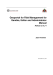
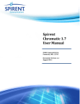
Chapter 21: Basic Ribbit
Introduction
Ribbit is a data processing program written by Thales GeoSolutions (Pacific) to
provide data processing capabilities primarily for WinFrog data. This software
makes the processing of WinFrog data easier, quicker, and safer than using
various third party programs. (ASCII XYZ data can also be used in Ribbit, but
with limited functionality. More details on this below in the Data Input section).
There are 3 versions of Ribbit available: Basic Ribbit, Advanced Ribbit, and Ribbit
Cable and Pipeline. The differences between these programs lies in the addition
of a 3D Digital Terrain Model viewer (in both Advanced and Cable and Pipeline)
and the ability to generate Profile View Data Panels (in the Cable and Pipeline
version only).
Note: in this document the terms Ribbit and Basic Ribbit are used
interchangeably.
Ribbit is a standalone program designed to run on all 32-bit WindowsTM
platforms. It is highly recommended that Windows NTTM version 4.0 (with at
least Service Pack 4) is used. Data storage and memory usage may be maximized
during data processing; a minimum of 32 MB RAM and 1.0 GB of ROM need to
be available. The computer’s display should also be of a “higher” quality.
Although the software will operate on a computer equipped with an 800 by 600
pixel display, it is recommended that a 1024 by 768 pixel display be used. This
improves the quality of the various graphical displays found in Ribbit. The
software will not operate at a resolution lower than 800 by 600 pixels.
Although Ribbit can be operated simultaneously with WinFrog on the same
computer, this is not recommended. Not only will the performance of the
programs suffer, conflicts within the operating system may also cause fatal
system crashes. However, data processing with Ribbit should not be left until the
end of the project either. It is important to verify both data quantity and quality
while there is still an opportunity to correct for any shortcomings.
This chapter deals with all aspects of using Ribbit for data processing, in the order
that they are found in the program. You may determine that your processing
efforts are better undertaken utilizing the various tools in a different order. For
example, you may wish to edit each individual data type before any merging or
modifications are undertaken (as opposed to the order that these steps are found
below). Although Ribbit is flexible in accepting these varied approaches, note that
there is no “undo” button available to quickly reverse your actions.
WinFrog 3.2 User’s Guide – Basic Ribbit
21-1
To aid with training, a sample data set is included with the Ribbit installation
kit. It is installed in the Samples directory, within the Ribbit directory. (i.e.,
C:\Program Files\Thales GeoSolutions (Pacific)\Ribbit\Samples). This data set
allows you to experiment with the software and to explore its features prior to
editing “real” data. The data are from a small hydrographic survey conducted in
San Diego, California in April 1997, and consist of data from a NMEAcompliant DGPS receiver (Leica MX400) and a NMEA-compliant echosounder
(Furuno FCV-582).
As with all Thales GeoSolutions (Pacific) software, Ribbit is in a constant state
of change and improvement. Select Help > About Basic Ribbit to see which
version of the program you are operating.
An Overview of Ribbit
Start Up
The Basic Ribbit program is included with all WinFrog installation disks; this
version of the program is provided as “freeware” and subsequently does not
require the use of any security devices at startup.
Ribbit generates the same display each time the program is started, as seen
below.
21-2
WinFrog 3.2 User’s Guide – Basic Ribbit
In fact, Ribbit is also internally configured the same way each time the program
is started. This differs from WinFrog which retains all configuration changes
each time the program is stopped, then recalls the configuration when the
program is started next. Each time a Ribbit session is closed, the program deletes
(i.e. “forgets”) all data input and editing configurations.
Upon each startup the Status window, the Audit Trail window, and the Toolbar
are displayed in the same locations. The following sections detail each of these
items.
Status Window
The Status window is displayed on the right side of the screen (as seen below)
for the duration of a processing session.
This window continually displays the names of the loaded Data Sets, the
amount of RAM and Page File Space available, and the Duration of the current
processing session.
The data field at the top of the Status window lists the WinFrog data records
currently held in memory and available for processing by the available tools. The
specific data items contained within these records are not listed.
WinFrog 3.2 User’s Guide – Basic Ribbit
21-3
The current available memory (RAM) and the available page file space are
displayed to provide you with information advising how close the computer is
operating to its memory capacity. Ribbit accepts as much data as memory allows,
but can become sluggish if the amount of available RAM is low and the page file
is being used for data storage. You can decide how much data Ribbit can handle
on the computer by watching the status window RAM value. This helps
determine when it might be more efficient to process data as several separate
data sets instead of one large data set.
Audit Trail “Notepad”
The Audit Trail is displayed as a yellow Notepad on the left-hand side of the
screen for the duration of a processing session, as seen below.
This window displays a local audit trail that lists a time tag of all events that
have taken place since the processing session began. Items included in the Audit
Trail are the names of loaded data files, which raw records have been selected for
processing, what modifications have been made to the data, etc.
You can scroll through the audit events for the current processing session, using
the scroll bar on the right side of the window.
The Audit window has an associated audit file. As each audit entry is made in
the on-screen Audit window, an audit entry is also made in an audit file
contained in the Ribbit processing directory. This audit file (audit.trl) is
automatically created in the Ribbit directory when Ribbit is first started. If the
audit file already exists, the audit data from each successive processing session
21-4
WinFrog 3.2 User’s Guide – Basic Ribbit
are appended to the file. Because each session is appended to the audit file, the
file can become quite large. You can periodically copy and rename the audit file
and then delete the original to decrease its size.
Menu Items
File, Edit and Search
The File, Edit and Search pull-down menus contain options related to text
editing of ASCII files. These options behave in the same way as similar menu
items found in standard word processors or in Windows® NotePad and are
provided to allow manual editing and inspection of WinFrog data files. The File
| Open menu item enables you to select a file from among the common
WinFrog file types and to open it into the text editor. Once a file is open it may
be edited directly. The Cut and Paste commands under the Edit menu and the
Find and Replace commands under the Search menu may be used to assist in
editing. These commands behave in exactly the same manner as the similar
commands in the Windows® NotePad program. Data files may be printed using
the standard Print, Print Preview and Print Setup commands. In most cases
these menu items represent a relatively minor set of functions that are rarely
used during a typical Ribbit processing session.
System Configuration File -- Load
When you select File | System Config File … | Load, a Standard Windows
‘open file’ dialog box is opened, enabling you to pick the cfg file to be loaded into
the current Ribbit processing session.
After the operation is complete you are notified with a message indicating the
configuration file has been loaded.
This operation will update the existing Ribbit initialization file with the
information in the selected configuration file.
System Configuration File – Save
When you select File | System Config File … | Save, a Standard Windows
‘save file’ dialog box is opened, enabling you to pick the cfg file to be saved to
disk. After the operation is complete you are notified with a message indicating
the configuration file has been saved.
This operation will save the existing Ribbit initialization file to the selected
configuration file.
Project Directories
When you select File | Project Directories, a dialog box is opened enabling you
to select the ‘Data Directory’ and the ‘Output Directory’ for Ribbit to use for
WinFrog 3.2 User’s Guide – Basic Ribbit
21-5
processing. Select the ‘Browse’ button for each operation to open a Standard
Windows ‘select folder’ dialog box to select the appropriate directory.
Data Input, Tools, and Data Output
These menu items (Data Input, Tools, and Data Output) provide access to all of
Ribbit’s processing functions.
Ribbit’s Data Input dropdown menu provides you the ability to input both
WinFrog and generic ASCII XYZ data types. See the Data Input section below for
complete details on all of these Ribbit data input tools.
Ribbit’s Tools dropdown menu provides you with various numerical and
graphical data editing functions including; tools for managing the individual
data records, merging one data type with another data type, interpolating data
based on specified time intervals, applying corrections to the data, filtering the
data, and changing the geographic coordinate system to which position data are
referenced. See the Tools section below for complete details on all of these Ribbit
processing tools.
The Data Output dropdown menu contains three different output utilities that
allow you to create an ASCII text file, a DXF format plan view map, and a
Microsoft AccessTM .mdb format data file. See the Data Output section below for
complete details on all of these Ribbit output functions.
Help
Currently, the Help >Contents functionality is not yet in place and details which
version of the program is being used.
Data Input
Ribbit’s Data Input dropdown menu allows you to input WinFrog and ASCII X,Y,Z
data types. Furthermore, three different WinFrog data formats can be imported:
Automatic Event data (.dat, .rcv, .src), Manual Event data (.log), and Raw (.raw)
data. Input of ASCII text also provides the following options: X,Y,Z (i.e. Easting,
Northing, Elevation), Y,X,Z or PC Time, Latitude, Longitude, Elevation. ASCII
data must be in comma or space separated format. You can also load data files in
the MS AccessTM (.mdb) format. These database files contain Time, Position, and
additional data.
The following sections detail each Data Input option.
Raw (.Raw) Files
Most data processing efforts use WinFrog’s raw (.raw) format data files. Since
21-6
WinFrog 3.2 User’s Guide – Basic Ribbit
the .raw data are truly “raw” in nature (i.e. no filtering or offsets are applied to
the data), these files often provide a better “base” starting point for processing
than would automatic event data.
Also, because WinFrog can be configured to record .raw data from devices as
quickly as it is able (as opposed to some specified time or distance interval),
these files can also provide a much larger volume of data to work with. See the
Eventing chapter for details on how to collect .raw format data using WinFrog.
In order to fully appreciate the flow of data into and out of a Ribbit processing
session, it is important that you become familiar with the WinFrog raw file format.
This format is simply a line-by-line list of all of the data from each individual
instrument interfaced to WinFrog, logged record-by-record, and preceded by an
identifying device code, the name of the device, and a time-stamp. An example
of the format, taken from a WinFrog .raw file, is as follows:
303,MX400,861879726.45,65126.00,32.71174000,-117.22566000,2,6,1.4,1.40,-33.30,6.30,262
This is a raw record from a Leica MX400 DGPS receiver. The data are preceded
by the code 303, which is the code for data output from a GPS receiver. Each
type of device has its own preceding code. For example, an echosounder has a
WinFrog code of 411, a digital compass or gyro has a code of 410, and so on. See
the WinFrog File Formats appendix for a detailed description of these files and
codes.
The next field contains the name of the device selected when it was first added.
In this example, it is MX400. See the Adding a Device section in the Peripheral
Devices chapter for details.
Following the name is the time-tag, which is a single number referred to as PC
time. PC time is a common method of representing time in data files and
represents the number of seconds elapsed since 00:00:00.0, January 1, 1970.
These first three fields of the raw data record are common to all devices.
The remaining fields in the raw file record are specific to the type of device
creating the record. For example, the 303 record includes fields for GPS Time of
Week, Latitude, Longitude, Status, Number of Satellites, HDOP, Altitude, etc.
Each individual line of data in a file is referred to as a data record, or record.
Each record can contain several fields, where a single value within a field is
referred to as a data item.
The WinFrog File Formats appendix contains specific details on the contents of
every raw data record produced and recorded by WinFrog.
WinFrog 3.2 User’s Guide – Basic Ribbit
21-7
Loading Raw (.Raw) Data Files
As briefly mentioned above, the various options found under the main menu
item Data Input are used to load files into Ribbit.
To Load WinFrog Raw (.raw) Files
1
Choose the Select RAW data files... option from the Data Input dropdown.
This action opens the Raw File Manager as seen in the next figure.
The Raw File Manager provides two methods for loading .raw files into the
current data processing session: Hand Pick and Time Pick. As the name
suggests, Hand Pick allows you to select .raw files manually, i.e. “by hand”
and Time Pick is used to select .raw files by specifying a time window.
To Hand Pick .Raw Files
1
In the Raw File Manager window, click the Hand Pick button.
2
Navigate to the directory containing the files.
Note: see WinFrog’s main menu item File> Select Working Directories to see
where the .raw data files were recorded. WinFrog’s default configuration
places .raw data files in the C:\ Navdata directory.
21-8
WinFrog 3.2 User’s Guide – Basic Ribbit
3
Select the desired .raw files.
Use the keyboard’s Shift or Ctrl keys to select multiple .raw files
simultaneously.
4
Click Open.
5
Ribbit “reads” the selected .raw files and lists all of the different Data Records
found in these files. Select the desired Available Data Records from the upper
right-hand list.
6
Click Add to move the selected items to the Working Data Records list.
Alternatively, double-click on the desired item in the Available Data Record
list to move that item to the Working Data Records list; or click the Add All
button to move all items in the Available Data Record list to the Working
Data Records list.
If you change your mind and want to remove a Data Record from the
Working Data Records list, you may do any of the following:
• highlight the item(s) in the list and click the Remove button to remove
those selected items;
• double-click on the item in the list to remove that one item; or
• click the Remove All button to remove all the data records from the list.
7
Click OK. Ribbit now closes this window and displays “Loading Data.... “
while it loads the Data Records into the temporary memory. Note that the
Audit Trail lists the selected .raw files and Data Records. The Status Window
also displays all loaded Data Records.
To Time Pick .Raw Files
1
In the Raw File Manager window, click Browse.
2
Navigate to the directory containing the files.
see WinFrog’s main menu item File> Select Working Directories to see
where the .raw data files were recorded. WinFrog’s default configuration
places .raw data files in the C:\ Navdata directory
Note:
3
Click OK.
4
Enter a Start time and End time.
Note: the time must be entered in the mm-dd-yy hh:mm:ss.s
5
format.
Click the Time Pick button.
Only those .raw data files created between the designated start and end times
(and residing in the current directory) are loaded into the Raw File Manager.
WinFrog 3.2 User’s Guide – Basic Ribbit
21-9
Once the desired .raw files have been loaded into the Raw File Manager, the
upper right list of Available Data Records will contain all of the data records
available from the selected files. The next step is to select which Data
Records are to be loaded into the current processing section.
6
Select the desired Available Data Records from the upper right-hand list.
7
Click Add to move the selected items to the Working Data Records list.
Alternatively, double-click on the desired item in the Available Data Record
list to move that item to the Working Data Records list; or click the Add All
button to move all items in the Available Data Record list to the Working
Data Records list.
If you change your mind and want to remove a Data Record from the
Working Data Records list, you may do any of the following:
• highlight the item(s) in the list and click the Remove button to remove
those selected items;
• double-click on the item in the list to remove that one item; or
• click the Remove All button to remove all the data records from the list.
8
Click OK.
Ribbit now closes this window and displays “Loading Data...” while it loads
the Data Records into the temporary memory. Note: the Audit Trail lists the
selected .raw files and Data Records. The Status Window also displays all
loaded Data Records.
Data (.Dat, .Rcv, .Src) Files
WinFrog’s Data files refer to those files generated when Automatic Eventing is
enabled, and include the .dat, .rcv, and .src Record Types. Each of these three
Record Types can be loaded by using the Select .DAT Data Files utility. Ribbit
places these three different Record Types into the same category because the files
are identical in structure and content.
WinFrog’s Automatic Event data differs from .raw WinFrog data in that they do
not represent data from any particular instrument, but rather represent the
instantaneous state of navigation of a particular vehicle at the moment of the
event. WinFrog events are discrete snapshots of the overall state of the vehicle,
recorded at either specified distances along a survey line or at specified time
intervals.
See the Eventing chapter for more details on data collection and data files.
21-10
WinFrog 3.2 User’s Guide – Basic Ribbit
To Load .Dat, .Rcv and .Src Data Files
1
From the Data Input menu, choose Select DAT data files ....
2
From the Files of Type dropdown menu, select the desired file type.
3
Navigate to the directory containing the desired file(s).
By default, WinFrog will place all of these data file types in the C:\ Navdata
directory. See WinFrog’s main menu item File >Select Working Files to
ascertain where these files are located.
4
Click Open.
Ribbit lists the loaded files in the Audit Trail Notepad and the Status window.
Manual Event (.Log) Files
WinFrog Manual Event files refer to those files containing data recorded
manually at a specific point in time as defined by the user. Manual Events are
stored in the Working .log file.
To Load Manual Event (.Log) Files
1
From the Data Input menu, choose Select .LOG event files ....
2
Navigate to the directory containing the desired file(s). By default, WinFrog
will place all of these data file types in the C:\ Navdata directory. See
WinFrog’s main menu item File >Select Working Files to ascertain where the
.log files are located.
4
Click Open.
Ribbit lists the loaded files in the Audit Trail Notepad and the Status window.
XYZ Data
XYZ Point files are files that can contain any number of fields which have XYZ
or Lat,Lon, Z datafields.
A dialog box is displayed when you select Data Input | Select XYZ Point Files.
This dialog box is a standard Windows ‘Add Files’ box which allows you to
select the drive, directory and filename. All filenames are displayed. Doubleclick a filename or click a filename and click Open to add the file to the current
Ribbit processing session . This dialog box is as follows:
WinFrog 3.2 User’s Guide – Basic Ribbit
21-11
The next step is to choose the appropriate options that match the input file. The
options supported are Code, Label, Edit Flag, Time and various forms of XYZ
or LatLonZ. An example is indicated below:
Selecting too many options for the selected input file will result in a message box
like the following sample.
21-12
WinFrog 3.2 User’s Guide – Basic Ribbit
Selecting too few options for the selected input file will result in a message box
like the following sample.
While XYZ files are loading, you are presented with a message like the one
below.
Loading Tide Files
Ribbit is capable of loading and utilizing tide data from three different sources;
Micronautics, Inc.’s World Tide program, the U.S. National Oceanographic and
Atmospheric Administration (NOAA), and “generic” ASCII files.
World Tide files are identified by their .tab extension, while NOAA’s files use the
.tid extension. The “generic” user-defined ASCII text format files can have any
extension type.
before any tide data are loaded into Ribbit, it is critical to confirm what
units of measure (i.e. meters or feet) and time reference (i.e. local or UTC) are
used in the tide file. It is also critical to confirm the same information for the
water depth data to which the tides will be applied.
Note:
ASCII Files
This method allows you to use tide files made up of simply ASCII text time and
tide data. This data can be in various formats, as specified below in the ASCII
Tide Input dialog box.
To Load an ASCII Tide File
WinFrog 3.2 User’s Guide – Basic Ribbit
21-13
1
From the Data Input menu, choose Tide Files ....> ASCII tide format.
2
Navigate to the directory containing the desired file.
3
Select the desired file.
(As mentioned above, any file extension will be accepted).
4
Click Open.
The ASCII Tide Input dialog box opens, as seen in the next figure.
The Example from input file window displays the contents of the first line in
the selected file.
5
Configure the Input format using the example as a guide.
6
Click OK to load the tide data and close this window.
World Tide (.Tab) Files
The World Tide program is used to generate predicted tides for any time period
at thousands of locations covering the entire globe.
To Load a World Tide (.Tab) File
21-14
1
From the Data Input menu, choose Tide Files ....> WorldTide ’TAB’ file.
2
Navigate to the directory containing the desired World Tide (.tab) file.
3
Select the desired .tab file.
4
Click Open.
WinFrog 3.2 User’s Guide – Basic Ribbit
NOAA Tide Files
The U.S. NOAA organization generates actual and predicted tide information
for any time period at hundreds of locations covering the coastal United States.
These NOAA (.tid) files can be downloaded from the NOAA web site.
To Load a NOAA (.Tid) Tide File
1
From the Data Input menu, choose Tide Files ....> NOAA tide format.
2
Navigate to the directory containing the desired NOAA (.tid)file.
3
Select the desired .tid files.
4
Configure the following parameters of the NOAA Tide Input dialog box:
Data Source
Station Code
Gauge number
Enter the code for the tide station.
The number of the gauge (typically 1).
Quality
Use Flagged data?
Max Std Dev:
WinFrog 3.2 User’s Guide – Basic Ribbit
Tide data are time stamped similar to the
way .raw data are time stamped. If anything
abnormal occurs at a specific time stamp
that might make the data suspect, that data
are flagged. You can choose to use the
flagged data or not.
When data are flagged, they are assigned a
standard deviation that statistically describes
how far the data may deviate from the truth.
If you decide to use flagged data, you can
21-15
enter a standard deviation threshold so that
suspect data are not used.
Corrections
Time correction:
Scale:
Offset:
5
Alters the time of the data when it is loaded.
Scales the data by a constant value when
loaded.
Adds a constant value to the data when
loaded.
Click OK to load the data.
Note: if it appears that the data are not loaded, check to ensure that the
Station Code and Gauge Number are correct.
MS Access (.Mdb)Data
Microsoft’s AccessTM is a program used in various database applications,
including Thales GeoSolutions (Pacific) Inc.’s WinFrog and Cable Route Design
Database (CRDD) software systems. The files generated and used by MS
AccessTM are identified by a .mdb extension.
To Load an MS Access (.Mdb) File
1
From the Data Input menu, choose Input From MS Access Database.
2
Navigate to the directory containing the desired .mdb file.
3
Select the desired .mdb file.
4
Click Open to close this window and load the file.
Clear Data
Clicking on this menu item when data is loaded in Ribbit will prompt you with
the following dialog box:
Select OK to clear all data from memory or Cancel to perform other Ribbit
actions.
21-16
WinFrog 3.2 User’s Guide – Basic Ribbit
Tools
The Tools menu is used to access 10 different functions that allow you to
manipulate the Data Records and Data Items presently loaded in Ribbit. All
changes made to the loaded data records or items are recorded in the Audit Trail
Notepad window.
Note: as previously mentioned, at no point are the
contents of the original data
files overwritten to reflect the modifications made using any of Ribbit’s tools.
Data Operations
This tool allows you to determine the number of Data Items contained in each
Data Record, as well as ascertain the Minimum and Maximum values of these
Data Items. It also provides you with a value that summarizes the percentage of
Data items that have been flagged as Edited Out. The Data Operations tool also
allows you to rename loaded Data Items and delete, rename, and copy loaded
Data Records.
To Perform Data Operations
1
From the Tools menu, choose Data Operations.
The Data operations and information window appears as seen in the next
figure.
Available Records and Data Items
This window lists all Data Records and Data Items loaded in the current
processing session.
WinFrog 3.2 User’s Guide – Basic Ribbit
21-17
Information
Details the specifics for any Data Item in the Available Records and Data
Items list. Double click on any Data Item to display the following
information:
!
!
!
!
!
!
Data Item Name
Source Record
Number of Items
Maximum Value
Minimum Value
% Edited Out
Delete Record
Copy Record
Rename Record
Rename Data Item
21-18
This function allows you to delete any
loaded Data Record.
To delete a Data Record, first click on the
desired Data Record (found in the Available
Records and Data Items list), then select
Delete Record. A Confirmation required
message appears at this point. Select Yes to
delete the selected Data Record.
This function allows you to copy any loaded
Data Record.
To copy a Data Record, first click on the
desired Data Record (found in the Available
Records and Data Items list), then select
Copy Record. The Copy Data Set dialog box
appears. Enter a name for the new Data
Record, then select OK.
This function allows you to rename any
loaded Data Record. This is required when
more than one Data Record of the same type
has been added, as Ribbit is unable to
differentiate between Data Records with
identical names.
To rename a Data Record, first click on the
desired Data Record (found in the Available
Records and Data Items list), then select
Rename Record. The Information Required
dialog box appears. Enter the new name for
the Data Record, then select OK.
This function provides you the means to
rename any loaded Data Item. This is
required when more than one Data Item of
the same type has been added, as Ribbit is
unable to differentiate between Data Items
WinFrog 3.2 User’s Guide – Basic Ribbit
with identical names.
To rename a Data Item, first click on the
desired Data Item (found in the Available
Records and Data Items list), then select
Rename Data Item. The Rename Data Set
dialog box appears. Enter the new name for
the Data Item, then select OK.
Note: do not change the record number
type. Ribbit requires this information to
identify what type of data item it is.
Merging / Deskewing
The Data Merging and Deskewing Tool is used to interpolate values from one
Data Item to the time stamps of another Data Item. This merging operation is
used to unify multiple, separate Data Items into a single new Data Item.
All data merging performed in Ribbit is based on a linear interpolation over
time. Depending on which Data Item is merged “to”, the data density of the new
Data Item can increase, decrease, or remain the same. For instance, merging a
raw Depth Data Item to a raw Position Data Item will typically reduce the
number of depth measurements that will be used for subsequent processing.
This is due to the fact that Echosounders typically output numerous depths per
second (depending on water depth), whereas Positioning Devices typically are
not capable of data output at more than once a second. Merging in this
“direction” will result in a new Data Item containing the same number of
records as contained in the Positioning Data Item (i.e. Ribbit will interpolate a
depth value for the time stamps of each position).
On the other hand, you can merge a Position Data Item to a Depth Data Item to
get a Position to match each Depth measurement. In this case Ribbit is creating
extra positions to match each depth measurement time stamp.
Ribbit will interpolate between chronologically successive Data Items that are
separated by less than the time set in the Maximum time gap box (entered in
seconds). This helps eliminate interpolation errors that occur when
interpolating over large time periods.
To Merge Data Items
1
From the Tools menu, choose Merging/deskewing. The Merge/de-skew
interpolation Control dialog box opens.
WinFrog 3.2 User’s Guide – Basic Ribbit
21-19
2
Double-click the desired Data Record or Data Item in the Interpolate FROM
list. The selection now appears in the Interpolate field at the bottom of the
Interpolate FROM list.
Note: selecting a Data Record will result in Ribbit merging all Data Items in
that Data Record. It is preferred to merge single Data Items.
3
Double-click the desired Data Record or Data Item in the Interpolate TO list.
The selection now appears in the Interpolate field at the bottom of the
Interpolate TO list.
Note: selecting a Data Record will result in Ribbit merging all Data Items in
that Data Record. It is preferred to merge single Data Items.
4
Type a unique name in the to produce field at the bottom of the Available
Data Items list.
5
Enter a Maximum time gap value (in seconds) in the provided window.
Note: checking the Combine Data checkbox will cause the selected data to be
combined with no interpolation.
21-20
6
Click Perform the Interpolation. Notice that the new Data Item now appears
in the Available Data Items list. The name is as specified above, while the
record number is created by Ribbit.
7
Click Done to close this window and return to the main Ribbit display.
WinFrog 3.2 User’s Guide – Basic Ribbit
Interpolation
The Interpolation tool allows you to create new data values via the linear
interpolation of the time stamps of existing data. The interpolation is similar to
the Merging/Deskewing tool in that the interpolation is based on time. However,
it interpolates within a specific data record instead of from one record to
another.
The Data fill-in interpolation dialog window provides two methods of record
interpolation:
1
Interpolate a new value to edited out points initiates the creation of a new
data value for each Edited Out data point, based on the nearest valid data
points before and after the Edited Out data point being interpolated. This
feature effectively generates new “good” data based on the time stamp of a
“bad” data point.
2
Interpolate a new value based on time initiates the interpolation of a new
value to a user-specified Time interval. For example, if raw GPS data was
collected every 10 seconds, but positioning data is required every 5 seconds,
this tool would be used to generate the new data points. As with the method
mentioned above, data interpolation is based on time.
Data created using either interpolation technique can be flagged as Edited Out
using the check-box selection. This allows you to identify the data as “nonoriginal” data. A Maximum time-interval for interpolation can also be set.
WinFrog 3.2 User’s Guide – Basic Ribbit
21-21
To Interpolate Data
1
From the Tools menu, choose Interpolation. The Data fill-in interpolation
dialog box appears as seen below.
2
From the Available data list, double click the desired Data Record. The item
will appear in the Selected data window below.
3
Select one of the two options mentioned above. If Interpolate a new value
based on time is selected, enter a Time interval value in seconds.
4
If desired, enable the Flag new points as ’edited out’ option. (Typically this
is selected).
5
Enter a Maximum Time interval (in seconds).
6
Click on the Do Interpolation... button.
7
Click Done to return to the main Ribbit window.
Apply Corrections
The ability to apply corrections to loaded Data Items is one of the most
commonly used features in Basic Ribbit. Three different forms of corrections can
be applied:
! the addition of a constant value to selected data
! the multiplication of selected data by a constant value
! the addition or subtraction of hours/minutes/seconds from the time-tag
of selected data
It is recommended that you undertake these operations independently to ensure
that the corrections are applied in the desired order.
21-22
WinFrog 3.2 User’s Guide – Basic Ribbit
To Apply a Correction to a Data Item
1
From the Tools menu, choose Apply Corrections.
2
From the Available data items list, double click on the desired Data Item.
3
In the Correction to apply area, check the desired box.
4
Enter the desired correction value(s).
To subtract a constant from the selected Data Item, select Add to value and
type in a negative value.
To divide the selected Data Item, enter a value of 1/constant.
5
If Time Correction is selected, select either the Add or Subtract radio button.
6
Click Perform Operation.
Filtering & Thinning
The Filtering & Thinning tool is primarily used to reduce (thin) the volume of
data from a selected Data Item. This thinning is accomplished by gating out
noisy data and removing outliers based on statistical modeling. The points that
are filtered or discarded can be removed entirely or alternatively flagged as
“edited out,” allowing you to reinstate (“edit in”) individual points later, if
desired. When executing the Filters option, a third option for the filter results,
WinFrog 3.2 User’s Guide – Basic Ribbit
21-23
Create new Filtered data set, is available. When this option is selected, the filter
is applied, but as the filter moves through the data set, instead of the results of
the filtered subset being used to test a given data point to determine if it lies
within the specified tolerances, the filtered data point is added to a new data set,
resulting in a new data set of filtered points.
Note: the “Action” (Remove record entirely or Flag as ‘edited out’) and Data To
Use selections must be made before any tools found in this window are utilized.
The Action selection defines whether the data points selected by the filtering and
thinning tools will be deleted or simply flagged as “edited out.” The Data To Use
selection allows you to include (or exclude) data that have previously been
deemed “edited out.”
To Thin Out a Data Item
1
From the Tools menu, choose Filtering & Thinning.
The Crude Discard selection provides you with the ability to define the
quantity of data to be removed or edited out.
2
From the Available Records and Data Items: list, double-click the desired
Data Item.
The name of that particular Data Item now appears in the Selected Data
21-24
WinFrog 3.2 User’s Guide – Basic Ribbit
field at the bottom of the Available Records and Data Items: list.
3
In the Data Record Tools area, click the Crude Discard radio button.
4
Move the mouse pointer to be precisely on top of the slide bar, then (while
holding down the left mouse button) move the bar to set a value between 2
and 10. This value indicates the amount of data to be removed (i.e. 2
indicates that 1 in 2 points in the selected Data Item will be removed or
flagged as “edited out”).
5
In the Action area, select either the Remove record entirely or Flag record as
‘edited-out’ radio button.
6
In the Data to Use area, select either the Use all data or Do not use ‘editedout’ data radio button.
7
Click Perform Operation.
To Filter a Data Item
1
From the Tools menu, choose Filtering & Thinning. The Data Item Tools
section of the Filtering and Thinning window provides you with four
mathematical methods that can be applied to remove or edit out data from
the selected Data Item.
!
!
!
!
Gate Filter
Mean Filter
Median Filter
Central Tendency
Gate Filter
The Gate Filter is used to filter out all data that is over or under user defined
limits.
To Apply a Gate Filter to a Data Item
1
From the Tools menu, choose Filtering & Thinning.
2
From the Available Records and Data Items: list, double-click the desired
Data Item. That particular item now appears in the Selected Data field at the
bottom of the Available Records and Data Items: list.
3
In the Data Items Tools area, click the Gate radio button.
4
Check the Filter all values over box and/or the Filter all values under box.
5
Enter the appropriate gating value(s). Ribbit assumes this value to be in the
same units as the selected Data Item.
WinFrog 3.2 User’s Guide – Basic Ribbit
21-25
6
Click Perform Operation.
Mean Filter
Data Items can also be filtered using the Mean Filter. In mathematical terms a
mean value is the average value of all included points. The Mean Filter requires
the entry of a Filter accept width and Number of samples values.
The Number of samples is the total number of observations that are used to
determine the mean value. If an even value is entered (as per the default of 10),
Ribbit will calculate the mean of 10 accepted points total (5 accepted points
found before and 5 points after the point in question). If an odd value is entered
for the number of samples, the following points will include the “extra” point.
The point in question is not used in the mean calculation.
Ribbit then takes the calculated mean value and adds and subtracts the value
found in the Filter accept width to determine an upper and lower acceptance
value. The point in question is then compared to these acceptance values. If the
point falls outside the acceptance value window, it is either removed entirely or
flagged as edited out.
Alternatively, if the Create new Filtered data set option has been selected, the
results of the filter algorithm will be added to the new data set.
To Apply a Mean Filter to a Data Item
1
From the Tools menu, choose Filtering & Thinning.
2
From the Available Records and Data Items: list, double-click the desired
Data Item. That particular item now appears in the Selected Data field at the
bottom of the Available Records and Data Items: list.
3
In the Filters area, click the Mean radio button.
4
Enter values for Filter accept width: and Number of samples.
5
Click Perform Operation.
Median Filter
Data Items can also be filtered using the Median Filter. In mathematical terms, a
median value is a value that has an equal number of observations below and an
equal number of observations above it in the sample data set. The Median Filter
requires the entry of a Filter accept width and Number of samples values.
The Number of samples is the total number of observations that are used to
determine the median value. If an even value is entered (as per the default of
10), Ribbit will calculate the median of 10 accepted points total (5 accepted
points found before and 5 points after the point in question). If an odd value is
21-26
WinFrog 3.2 User’s Guide – Basic Ribbit
entered for the number of samples, the following points will include the “extra”
point. The point in question is not used in the median calculation.
Ribbit then takes the calculated median value and adds and subtracts the value
found in the Filter accept width to determine an upper and lower acceptance
value. The point in question is then compared to these acceptance values. If the
point falls outside the acceptance value window, it is either removed entirely or
flagged as edited out.
Alternatively, if the Create new Filtered data set option has been selected, the
results of the filter algorithm will be added to the new data set.
To Apply a Median Filter to a Data Item
1
From the Tools menu, choose Filtering & Thinning.
2
From the Available Records and Data Items: list, double-click the desired
Data Item. That particular Data Item now appears in the Selected Data:
field at the bottom of the Available Records and Data Items: list.
3
In the Filters area, click the Median radio button.
4
Enter values for Filter accept width: and Number of samples:
5
Click Perform Operation.
Central Tendency Filter
Data Items can also be filtered using the Central Tendency Filter. In
mathematical terms, a central tendency value is the value found at the center of
a line that is best fit through the sample data set. The Central Tendancy Filter
requires the entry of a Filter accept width and Number of samples values.
The Number of samples is the total number of observations that are used to
determine the central tendency value. If an even value is entered (as per the
default of 10), Ribbit will calculate the central tendency of 10 accepted points
total (5 accepted points found before and 5 points after the point in question). If
an odd value is entered for the number of samples, the following points will
include the “extra” point. The point in question is not used in the central
tendency calculation.
Ribbit then takes the calculated central tendency value and adds and subtracts
the value found in the Filter accept width to determine an upper and lower
acceptance value. Note: with this particular filter, the Filter accept width value
can be defined in the Gate Width Type section to be in Absolute Data Item units
or Statistical units of Sigma (one standard deviation).
The point in question is then compared to these acceptance values. If the point
falls outside the acceptance value window, it is either removed entirely or
WinFrog 3.2 User’s Guide – Basic Ribbit
21-27
flagged as edited out.
Alternatively, if the Create new Filtered data set option has been selected, the
results of the filter algorithm will be added to the new data set.
To Apply a Central Tendency Filter
1
From the Tools menu, choose Filtering & Thinning.
2
From the Available Records and Data Items: list, double-click the desired
Data Item. That particular Data Item now appears in the Selected Data:
field at the bottom of the Available Records and Data Items: list.
3
In the Filters area, click the Central Tendency radio button.
4
Enter values for Filter accept width and Number of samples. As mentioned
above, use the Gate Width Type radio buttons to change the Filter accept
width from Data Item units to statistical units of Sigma.
5
Click Perform Operation.
Change Geodetics
The Change Geodetics tool allows you to convert the geodetic parameters
(reference ellipsoid, datum shifts and map projection) of a loaded positional
Data Item. There are 4 conversions that can be undertaken using this tool.
1
Positional Data Items recorded as WGS84 referenced lat/long coordinates
can be converted to lat/long referenced to another datum or to map
projection Northing/Easting coordinates.
2
Positional Data Items recorded as non-WGS84 referenced lat/long
coordinates or map projection Northing/Easting coordinates can be
converted to WGS 84 lat/long coordinates.
Note: errors made in the specification of geodetic constants will be carried
throughout an entire survey and can have disastrous results. Therefore, it is
imperative that you understand the implications of modifying the geodetic
constants and ensure that all values are set correctly.
21-28
WinFrog 3.2 User’s Guide – Basic Ribbit
To Change a Data Item’s Geodetics
1
From the Tools menu, choose Change Geodetics.
2
From the Available Plan View Data Items: list, double-click the desired item.
This places the selected item into the Selected Plan View Data Item: field.
3
Click Change.
The Geodetics dialog box appears, identical to the one in WinFrog.
4
Configure the geodetics as desired.
5
When finished making the changes in the Geodetics dialog box, click OK to
return to Ribbit’s Geodetic Control dialog box.
6
Click the desired radio button.
Note: if you are converting from one non-WGS84 coordinate system to
another non-WGS84 coordinate system, you must first convert the data set
to WGS84 and then convert from WGS84 to the other working system.
7
Click the Apply Change to Data Item button.
8
Click Done.
WinFrog 3.2 User’s Guide – Basic Ribbit
21-29
Apply Offsets
Basic Ribbit’s Apply Offsets tool allows you to horizontally offset the coordinates
contained in any loaded positional Data Item. This is necessary when events
have been recorded in the field without having the correct Tracking Offset
enabled or perhaps incorrect offsets were entered in WinFrog’s Offsets window.
The most common use of this tool is to offset raw GPS antenna positions to the
location of the vessel’s echosounder. Without this offset calculation, the depths
will be incorrectly related to the GPS antenna position.
It is critical that any offset that is applied must use a gyro device Data Item for
heading information. The use of Course Made Good “headings” is only relevant
if the vessel is truly progressing in the same direction that the vessel is pointed.
To Apply a Horizontal Offset to a Positional Data Item
1
From the Tools menu, choose Apply Offsets.
2
Double-click the desired Data Item from the Available Plan data items: list.
(Only those data items containing horizontal positioning data are
presented).
This places that data item in the Selected data: field.
3
Enter the desired offset values into their appropriate boxes, along with the
appropriate mathematical sign: forward (+) or aft (-), starboard (+) or port
(-).
The Graphics window displays the direction of the entered offsets before they
are applied (Note: this is not to scale). This display helps eliminate errors
caused by entering in the wrong sign for offsets.
4
21-30
In the Heading Source area, click either the Course-Made-Good radio button
or the Heading data: radio button.
WinFrog 3.2 User’s Guide – Basic Ribbit
Course-Made-Good is calculated using consecutive positional measurements,
whereas Heading data: comes from raw heading observations recorded in the
field. The dropdown menu displays a complete list of all available Heading
Data items.
5
Click Calculate Offsets.
Overplot Removal
The Overplot Removal tool is used for creating hydrographic sounding charts in
which only a specific result is required, namely only the shallowest depths. It
performs a shoal-biased thinning of the soundings data. This means that the
data will be thinned to leave only one item within a specified radius, with this
record being the minimum (i.e. shallowest) sounding.
Because the Overplot removal tool filters a Z dimension based on its horizontal
X/Y coordinates, it is necessary to first convert one or two dimension Data Items
to a three dimension Data Item using the Interpolation tool. (i.e. interpolate a
Depth Data Item (one dimension) to a Position Data Item (two dimensions) to
generate an X/Y/Z (three dimensions) Data Item.
Furthermore, the resulting three dimensional data record must be in grid
Northing/ Easting coordinates. You must use the Geodetics tool to convert the
geographic lat/lon coordinates to grid coordinates before the overplot removal
tool can be used. Also, note that this operation can be time consuming for large
sets of data.
To Apply Overplot Removal to a Three Dimensional Data Item
1
From the Tools menu, choose Overplot Removal.
WinFrog 3.2 User’s Guide – Basic Ribbit
21-31
2
Double-click the desired Data Record as found in the Available records: list.
This places the record in the Selected data: field below the Available records:
list.
3
Enter a value in the No-plot radius: field.
Note: the units of the entered radius refers to the units displayed in the
Geodetics area of the Overplot removal dialog box.
4
Click Perform operation to execute the overplot removal.
This results in a new Data Record named Reduced. This data set contains
only the shoal-biased soundings.
Interactive Data Editor
The Interactive Data Editor allows you to graphically view and edit individual
Data Items loaded into the current processing session.
You can view up to two Data Items simultaneously; The first Data Item viewed
is called the Primary Data Item and the second is called the Secondary Data
Item. The Primary and Secondary Data Items must be from the same category.
For example, Plan data and Profile data cannot be viewed at the same time. Plan
Data Items are plotted by their Northing/Easting values, while Profile Data
Items are plotted in the Y-axis relative to time along the X-axis. Since Profile
Data Items can be edited in this way, this editor is also referred to as the TimeBased editor.
The Edit out feature allows for the removal of user selected data from the current
processing session, while the Edit in feature can be used to re-instate “edited out”
data.
21-32
WinFrog 3.2 User’s Guide – Basic Ribbit
To Edit a Data Item using the Interactive Data Editor
1
From the Tools menu, choose Interactive Data Editor.
2
Select the desired Data Item from the Primary dropdown menu.
Ribbit graphically displays the selected Data Item data. Ribbit automatically
centers the data and optimally scales the data to fit within the limits of the
display space.
3
If a second Data Item is to be viewed, select the desired Data Item from the
Secondary dropdown menu.
Ribbit does not automatically adjust the data scales for the second Data Item.
Therefore, it might not be visible without adjusting the graphic controls.
The graphic controls, located in the upper right panel of the Time-Based
Editor, provide you with the ability to Zoom-In and Zoom-Out as well as Pan
Left, Right, Up, and Down into a specified area.
4
If the Edit Out box is checked, individual data points can be “edited out” by
drawing a box around the particular point(s) with the cursor. (Hold down
the left mouse button while drawing the box).
A data point that has been flagged as “edited out” is displayed in gray
WinFrog 3.2 User’s Guide – Basic Ribbit
21-33
regardless of which Primary or Secondary Data Color has been selected.
Note: only Primary Data
Points can be edited. Also, remember that any
points flagged as “edited out” are not used in any subsequent processing or
final output results.
5
If points have been mistakenly edited out, they can be edited back into the
processing session by checking the Edit In box and then once again drawing
a box around the point(s) with the cursor. This returns the point to its
original color and re-includes the point in all subsequent processing.
6
The upper right-hand corner of the Time-Based editor displays Time and
Values and information specific to one Data Item, referenced to the cursor
position. This feature is enabled or by checking the Cursor Data box at the
bottom of the Time-Based editor.
7
You can force Ribbit to have the lower tool “tray” remain visible along the
bottom panel of the Time-Based editor by checking the Tray Up box at the
bottom of the Time-Based editor.
8
The Vertical Exaggeration function can be used to shows more detail in
items that have small vertical variances with respect to horizontal axis. The
Vertical Exaggeration is changed by clicking the Up or Down arrows.
9
Horizontal and vertical grid lines can be turned off or on in the display.
Display the grid lines by checking the Vertical grid box and the Horizontal
grid box.
10
Select the Primary Data Color and Secondary Data Color buttons to change
the color of the selected Data Item. The display’s background color can be
changed by clicking the Background Color button and selecting the desired
color.
Note: using a display with a resolution of less than 1024 by 768 pixels may
limit the availability of some of the features discussed above.
11
21-34
Click the X in the top right corner of the Time-Based Editor window (NOT the
corner of the entire Ribbit window) to close the Interactive Data Editor.
WinFrog 3.2 User’s Guide – Basic Ribbit
Spreadsheet Editor
As the name implies, the Spreadsheet Editor allows you to edit the contents of
any loaded Data Record through the use of a spreadsheet-style text editor. This
editing tool allows you to not only change the status of a data string, but to also
change the value of any Data Item contained in the selected Data Record.
To Edit a Data Item Using the Spreadsheet Editor
1
From the Tools menu, choose Spreadsheet. The Data Edit Selection window
appears as seen below.
2
Select the desired Data Record from the Available Data Items list.
3
Click on the Edit button. The Edit Data Items spreadsheet dialog box opens.
WinFrog 3.2 User’s Guide – Basic Ribbit
21-35
4
Use the slide bar found at the right side of the display to view additional data
strings. If you click on any data field in the spreadsheet editor, you can also
use the keyboard’s Page Down button to view additional data.
Use the slide bar found at the bottom of the display to view additional Data
Items contained in each of data string.
5
To change the status of a data string , i.e., to be included (in) or “edited out”
(out), click on the desired string’s Edit value, then use the dropdown window
to select the appropriate option.
6
To change the value of a particular Data Item, double-click on the desired
Data Item’s value, then use the keyboard’s left and right arrow buttons to
move to the appropriate digit. Now, simply enter the new value(s) as desired.
Note: all Data Item values, except Time, can be modified.
7
Once all editing is complete, click on the OK button to return to the Data Edit
Select dialog box.
8
Click on the OK button if you are finished editing.
Data Output
Basic Ribbit can output data in ASCII text, .DXF graphics, and MS AccessTM .MDB
data base formats. The Data Output menu provides access to each of these
utilities.
Note: if the ASCII text or .DXF graphics Data Output formats are selected, only
those Data Items with an “edited in” status will be included in the final output
product. MS AccessTM .MDB data base files retain all Data Item information,
including status.
ASCII File Output
ASCII files, also known as flat text files, are simple text files that can be read by
any text editor (such as WordTM, NotePadTM, WordpadTM), spreadsheet editor
(such as ExcelTM or LotusTM,) and even some mapping software systems (such as
AutoCAD’s QuicksurfTM).
Note: only individual Data Records may be exported using the Output to ASCII
feature. If you wish to export a combination of Data Items, you must first
interpolate one to the other using the Interpolation tool. Alternatively, individual
ASCII files can be combined using text or spreadsheet editors.
21-36
WinFrog 3.2 User’s Guide – Basic Ribbit
To Output Data as ASCII Text
1
From the Data Output menu, choose Output to ASCII file.
2
From the items in the Available Data Records: list, select the desired Data
Record to output into ASCII format.
The selected data record appears in the Selected data record: field. An
example of how that record will be formatted when it is output in ASCII
format appears in the Example: field. This example represents a single line of
data as it will be written to the ASCII file. This enables a quick check of the
format prior to actually writing the file. Changes made to any of the Options
available in the ASCII file out dialog box are instantly reflected in the
Example: field.
3
Check the desired options in the Options area.
Select Include Code to include the three digit record identifier or code.
Remember that each data record has a unique code to identify it from other
records.
Select Include Time to include the time recorded for every data item in that
record. Some data may have interpolated time values. The time can be in
either PC Time (in seconds from 00:00 on January 1, 1970), in regular
Day/Month/Year Hours:Minutes:Seconds format or in Month/Day/Year
Hours:Minutes:Seconds
Select Include Label to include the label for every data item in that record.
This information can be useful to identify each record by number.
WinFrog 3.2 User’s Guide – Basic Ribbit
21-37
Select Include ‘Edited Out’ Data to include an edited out value for each
record. This value will be ‘1’ for edited data records and ‘0’ for unedited data
records.
4
In the Delimiters area of the Options dialog box, check the ‘,’ Separator radio
button to create comma separated data fields or check the ‘ ’ Separator radio
button to create space separated data fields.
5
Set the precision of the output data from 0 to 8 decimal places by placing the
mouse pointer precisely on top of Precision slide bar then, while holding the
left mouse button down, move the bar to the desired setting.
6
Click the Browse button to navigate to the desired location where the new
file will be created and to define the name of the new file.
by default an .asc file extension will be added to the entered file name.
This can be changed to any desired extension if required.
Note:
7
Click OK at the bottom of the ASCII file out dialog box to generate the new
file.
DXF File Output
This Data Output option is used to generate plan view charts in the popular .DXF
format. As implied by the name, (an abbreviation for Drawing Exchange
Format), the DXF file format is used to exchange graphical data between various
CAD software packages including AutoCADTM, PageMakerTM, CorelDrawTM,
ArcViewTM, and MapInfoTM. These systems can then be used to modify the
contents of the DXF chart. DXF drawings can also be input into a Microsoft’s
WordTM document if equipped with the appropriate filter.
Note: all items depicted in the DXF charts created
by Ribbit are in real world
map projection coordinates.
The DXF charts created by Ribbit consist of multiple layers, with each layer
containing a separate component of the drawing.
Ribbit defines colors using the same numbering pattern as AutoCADTM, with
the basic colors numbered as follows:
1: Red 2:Yellow 3:Green 4:Cyan 5: Blue 6: Magenta 7:Black
To Create a DXF Chart
1
21-38
From the Data Output menu, choose Output to DXF file. The Hydrographic
Plan Plot dialog box is displayed, as seen below.
WinFrog 3.2 User’s Guide – Basic Ribbit
2
Select the appropriate Data Item from the Available Plan View Data Items
list. Only those Data Items containing positional data (i.e. Lat/Long or
Northing/Easting coordinates) are presented for selection.
Double-click on the desired Data Item to select it. The Selected Plan View
Data Item window will display the name of the Data Item chosen.
Note: if you select a Data Item that contains Latitude /Longitude
coordinates, you must ensure that the Configure Geodetics Tool is configured
correctly in terms of Datum and Zone before the DXF chart is created.
3
The Plot Information area options must be defined for each chart created.
These parameters define the size, rotation, and real world location of the
chart.
Center Northing:
Center Easting:
Rotation:
WinFrog 3.2 User’s Guide – Basic Ribbit
and
Enter the map projection grid coordinates of
the center of the chart. As mentioned above,
the coordinates cannot be specified in units
of latitude/longitude.
Enter a value to define the amount of
rotation that will be applied to the chart’s
border. As previously mentioned, the data
and grids depicted in the chart are always in
real world map projection coordinates, and
so are never rotated from their original
21-39
Intended Plot Scale:
Plot Length (mm):
locations. The rotation is entered in degrees
as measured clockwise from North.
Enter an integer value to define the scale
factor used in the chart. Entering a value of
1000, for example, tells Ribbit that 1 unit on
the chart will represent 1000 units in the real
world. This value is used to calculate the
size of the border and text items.
and
Enter the chart’s horizontal length and
vertical length dimensions. These values are
entered in millimeters, and together with the
scale determine the area that is represented
in the created chart.
Output DXF File:
Enter the name and location of the .DXF
file to be created.
Browse button
Opens a navigation dialog box where a new
file can be created or an existing file located.
Click the Layout Options button. The Plot Layout dialog box appears as seen
below.
Plot Height (mm):
3
21-40
WinFrog 3.2 User’s Guide – Basic Ribbit
The Plot Layout dialog window allows you to define if and how 2 grids, a
title, a border, and a North arrow will be plotted in the .DXF chart.
4
Configure the various Plot Layout options as desired.
if a dimension entry is requested in “units,” this refers to real world
units as opposed to plotted units; it may require some calculation to derive
the real world values. For example, if a grid annotation is to be plotted at a
size of 10 mm, with a chart scale of 1:1000, the “units” entry would be 10, as
determined by multiplying both values by a factor of 0.01.
Note:
Plot Projection Grid?
Check this option to generate a series of
projection grid Northing and Easting
“crosses” on the .DXF chart. You must
define the size of the annotations (Grid
Character Size in grid units), the size of the
grid “ticks” (Grid Tick Size in grid units), and
the spacing of the grid “ticks” (Grid Tick
Spacing in grid units).
You can also change the color of the grid
and annotation (Grid Color), the name of the
layer to which this information will be
written (Grid Layer), the AutoCADTM text
font (Grid Font), and the type of
AutoCADTM line that will be plotted (Grid
Line type).
Plot Latitude - Longitude
Grid?
Plot a Title?
Plot a border?
WinFrog 3.2 User’s Guide – Basic Ribbit
Check this option to generate a series of
latitude and longitude lines on the .DXF
chart. The options presented for this feature
are the same as those for the Projection grid
with one key difference; the Latitude and
Longitude Grid Spacing are specified in
minutes of arc rather than real world units.
For calculation purposes, 1 minute of arc is
approximately 1852 meters in length.
Check this option to plot the title entered in
the provided window (Title). You can also
define the Title Font, Title Character Size (in
real world units), the name of the
AutoCADTM layer on which the title is to be
placed (Title Layer), and the color of the title
text (Title Color as referenced to
AutoCAD’sTM color numbering ).
Check this option to plot a border around
21-41
5
6
21-42
the drawing. You can also define the border
width (Plot Border Width in real world
units), the color of the border (Border Color
as referenced to AutoCAD’sTM color
numbering), the name of the AutoCADTM
layer on which the border will be placed
(Plot Border Layer), and the separation
between the plot border and the overall
drawing limits (Border separation in mm).
Plot a North Arrow?
Check this option to plot a North Arrow.
You can define the color of the arrow (North
TM
Arrow Color as per AutoCAD’s color
numbering) and the name of the
AutoCADTM layer on which the north arrow
is to be plotted (North Arrow Layer). The
location and size of the North arrow are
automatically determined by Ribbit based on
the size and scale of the drawing.
Click OK to save these settings and return to the main Hydrographic Plan Plot
dialog window.
Click the Data Options button.
as seen below.
The Data Options dialog window appears
WinFrog 3.2 User’s Guide – Basic Ribbit
The Data Options dialog box controls what data will be included in the .DXF
chart and how the data are presented.
Include Direction Tics?
Plot 3D Data?
Post 3D Values as text?
Plot Time?
Plot DAT Events?
Merge with DXF Data?
WinFrog 3.2 User’s Guide – Basic Ribbit
Check this option to enable the drawing of a
line from each data point in the direction
equal to the vessel’s Course Over Ground at
that moment. You can define the length of
the line (Tic Size in real world units), the
name of the drawing layer to which the tics
will be written (Tic Layer), and the color of
the tics (Tic Color).
Check this option to enable the plotting of a
third dimension Data Item at each
positional data point,
i.e. a point in the DXF file will have X, Y,
and Z values rather than just X and Y plan
coordinates. The “Z” Data Item is selected
using the provided dropdown menu.
Check this option to have Ribbit plot the
value of the 3rd dimension (i.e. “Z”) Data
Item value beside the data point. You must
also select Plot 3D Data? above. See
Annotation options below to define how the
values will be appear on the chart.
Check this option to have Ribbit annotate
each data point with the time that that
particular event was recorded. Use the Time
reference: dropdown menu to select the
Data Item that will provide the time
reference.
Check this option to enable the plotting of
automatically generated event data (i.e.
those events generated by WinFrog based on
user-specified time or distance downline
intervals). Use the Event reference
dropdown menu to select the desired Data
Item.
Check this option to enable the plotting of
an existing .DXF file in the newly created
.DXF Chart. Only those features in the
selected existing DXF file that are within
the borders of the new DXF chart will be
added to the file being created, i.e., the
existing .DXF file will be cropped to the
21-43
7
8
21-44
area being plotted. Use the Browse button to
navigate to the desired .DXF file.
This portion of the Data Options window
Annotation Options:
provides you with the ability to customize
various annotation configuration options,
including; the size of the symbol that will be
plotted to represent that event (Symbol Size
in real world units), the annotation’s
character size (Character Size in real world
units), the offset of the annotation from the
data point (Text Offset in real world units),
the name of the layer that the Data Options
will be written to (Layer), the color of the
various Data Options (Color in AutoCADTM
numbering convention), and font of the
annotation (Font).
Basic Options
This portion of the Data Options dialog
window allows you to control the way that
the positional data will be plotted on the
.DXF chart. Select the appropriate radio
button to have Ribbit plot the data points as
Points, Lines, Circles, or Squares.
The Symbol Size box allows you to define
the size of the selected symbol; the entry
here (in real world units) defines a line’s
length, a circle’s radius or a square’s side
length. The name of the layer the points will
be added to and the color of the data can
also be modified by changing the
appropriate boxes.
Click OK to save these settings and return to the Hydrographic Plan Plot
dialog box.
Click the Setup Contours button. The Contour Options dialog box appears as
seen below.
WinFrog 3.2 User’s Guide – Basic Ribbit
The Contour Options dialog box is used to configure the plotting of contours
in the plan view .DXF chart. Contours are lines drawn joining points of
common elevation, hence only three-dimensional (i.e. “X/Y/Z”) Data
Records can be used. See the section above on Merging/Deskewing to create
three dimensional X/Y/Z data.
9
Double-click the desired Data Record in the Available Data Records list. The
Data Item name now appears in the Selected Data Item: field.
10
Configure the Contour Options as required.
Contour Interval:
Contour Layer:
Contour Color:
Label Contours?
Spacing
Text Color
Text Size
WinFrog 3.2 User’s Guide – Basic Ribbit
Enter a value (in the same units as the Z
data component) to define at what vertical
interval the contours will be generated.
Enter the name for the layer of the .DXF
chart on which the contours will be placed.
Enter a value to define the color of the
contours in the .DXF chart (as per
AutoCADTM color numbering).
Check this box to enable the annotation of
the contours with the appropriate elevation
value.
Enter a value to define the spacing of the
contour annotations.
Enter a value to define the color of the
contour annotations, as per AutoCADTM
color numbering.
Enter a value to define the size of the
contour annotations, in real world units.
21-45
11
Click OK to save these settings and return to the Hydrographic Plan Plot
dialog box.
At this point you should preview the .DXF chart to ensure that all of your
configuration entries were made correctly.
12
Click Preview Plot. Ribbit will generate a chart based on the various
configuration selections mentioned above.
13
Click Done to return to the Hydrographic Plan Plot dialog box.
14
If the chart appearance is suitable, click Create Plot button to create the
.DXF chart file in the pre-defined location. If the chart requires further
modifications, simply re-configure the appropriate dialog boxes as detailed
above.
15
Click Done to return to the main Ribbit window.
MS AccessTM .MDB File Output
.MDB files are database files created and utilized by Microsoft’s AccessTM
program. As the .MDB file format is one of the file types that Ribbit can input,
creating an .MDB file during a processing session provides you with a single
usable backup file of all currently loaded data. This could potentially save time
in future editing sessions.
Note: Ribbit writes all data to the .MDB file, regardless of status (i.e. even those
Data Items with an “edited out” status will be recorded to file.)
To Output Data to a .MDB File
21-46
1
From the Data Output menu, choose Output to MS Access Database. A
standard WindowsTM “Save as” dialog box opens.
2
Navigate to the appropriate directory and enter the desired file name. Ribbit
will add the .mdb extension automatically.
3
Click on the Save button to initiate the creation of this file and return to the
main Ribbit window.
WinFrog 3.2 User’s Guide – Basic Ribbit
This page intentionally left blank.
WinFrog 3.2 User’s Guide – Basic Ribbit
21-47