Download Bound-T Reference Manual - Bound

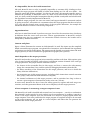
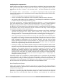
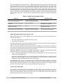
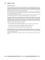
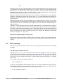
The -dot_dir option and the names of drawing files
The -dot option creates a single file that contains all drawings from one Bound-T run. If you
then use the dot tool to create a PostScript file, each drawing will go on its own page in the
PostScript file. However, dot can also generate graphical formats that do not have a concept of
"page" and then it may happen that only the first drawing is visible. If you want to use such
non-paged graphical formats it is better to create a directory (folder) to hold the drawing files
and use the Bound-T option -dot_dir instead of the option -dot. The -dot_dir option creates a
separate file for each drawing, named as follows:
•
The call-graph of a root subprogram is put in a file called cg_R_nnn.dot, where R is the
link-name of the root subprogram, edited to replace most non-alphanumeric characters
with underscores '_', and nnn is a sequential number to distinguish root subprograms that
have the same name after this editing.
•
If the call-graph of some root subrogram is recursive, Bound-T draws the joint call-graph of
all roots and puts it in a file called jcg_all_roots_001.dot.
•
The flow-graph of a subprogram is put in a file called fg_S_nnn.dot, where S is the linkname of the subprogram, edited as above, and nnn is a sequential number to distinguish
subprograms that have the same name after this editing and also to distinguish drawings
that show different flow-graphs (execution bounds) for the same subprogram.
The sequential numbers nnn start from 1 and increment by 1 for each drawing file; the same
number sequence is shared by all types of drawings and all subprograms. For example, if we
analyse the root subprogram main?func that calls the two subprograms start$sense and
start$actuate, with the -dot_dir option and -draw options that ask for one flow-graph drawing
of each subprogram, the following drawing files are created:
•
cg_main_func_001.dot for the call-graph of main?func
•
fg_main_func_002.dot for the flow-graph of main?func
•
fg_start_sense_003.dot for the flow-graph of start$sense
•
fg_start_actuate_004.dot for the flow-graph of start$actuate.
Call graphs
Figure 4 below is an example of a non-recursive call-graph drawing. The rectangles represent
subprograms and the arrows represent feasible calls from one subprogram to another. This
call-graph shows the root subprogram main calling subprograms Count25, Foo7, Foo and
Extract, some of which in turn call Count and Ones.
Each rectangle in Figure 4 is labelled with the subprogram name (in this example the compiler
adds an underscore '_' before the names), the number of times the subprogram is called, the
number of call paths, the execution time in the subprogram itself and the execution time of its
callees. The number of calls and the execution times refer to the execution that defines the
worst-case execution-time bound for the root subprogram.
In this example call-graph most subprograms have context-independent execution bounds
(same WCET bound for all calls). The exception is the subprogram Count which has some
context-dependent bounds. This can be seen from the annotation for the execution time of
Count: “time 1468 = 10 * 94 .. 158” which means that the execution time bounds for one call of
Count range from 94 cycles to 158 cycles, depending on the call path, such that the total bound
for the 10 executions of Count is 1468 cycles.
Call-graph drawings can become quite cluttered and hard to read when some subprograms are
called from very many places. For example, programs that do lots of trigonometry can have
numerous calls to the sin and cos functions. You can use “hide” assertions to omit chosen
subprograms from the call-graph drawing; see the Assertion Language manual.
Bound-T Reference Manual
Understanding Bound-T Outputs
87