Download Project Risk Analysis manual and tutorials

Project Risk Analysis by Katmar Software
Version 2.1
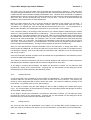
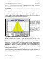
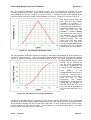
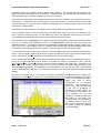
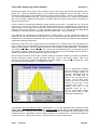
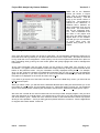
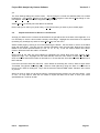
This cumulative probability (or
cdf) is useful because it tells us
very
quickly
what
the
probability is of being “less
than or equal to” the value
chosen.
When we are
estimating capital costs we are
not as interested in the
probability of the project being
exactly on budget as we are in
the probability of it being
within budget (ie on budget or
less).
Figure T1b - The Cumulative Probability Graph
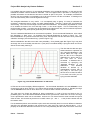
This process can be refined by making the sub-ranges narrower. This complicates the matter by requiring
the probability to be estimated for more sub-ranges. Eventually, as they get narrower and narrower, the
sub-ranges would become single points and a probability would have to be assigned to an infinite number
of points. This problem is solved by using a mathematical formula to calculate the probability for each
cost. This formula is called a statistical distribution, and all it does is give us a probability for each
possible cost.
This is why we made the claim that using statistical distributions is a natural process. It is basically a very
simple concept. Unfortunately it is made a bit more complex for people untrained in statistics by the use
of statistical jargon. There are a few terms that are used in connection with distributions that are worth
knowing. They are actually fairly simple concepts as well, and if you have not had much statistical training
(or if what you have had has got a bit rusty) please read through the rest of this section. You do not need
to remember all of it straight away. As you start using the Project Risk Analysis program it will re-inforce
the concepts and you will soon get used to them.
At this stage you should have a basic understanding of the concepts of a probability density function (pdf)
and a cumulative distribution function (cdf) as applied to costs. We are now going to progress to some of
the statistical distributions that are used in the PRA program, and to start introducing a few more statistical
terms. If you are not comfortable with the concept of a probability distribution you should read through the
first part of this tutorial again, particularly trying to understand what Figures T1a and T1b are telling us.
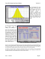
There are three new terms we will now define. These are Low Cost, High Cost and Likely Cost. For a
distribution like that shown in Figure T1a the Low Cost is the lowest cost found. In this case we see that
there is never a cost less than 5, and we would call 5 the Low Cost in this case (pretty obvious isn’t it?).
Similarly, the High Cost would be 10, because we never have a cost more than that.
The Likely Cost is the cost that occurs more often than any other particular cost, ie the cost that has the
highest probability of occurring. Figure T1a is a plot of Probability against Cost, so we can easily find the
highest probability by finding the highest point on the curve, and then reading off the corresponding cost,
which gives us the Likely Cost. In this case the Likely Cost is between 7 and 8. In statistical terms the
Likely Cost is called the mode. We will not use this terminology in PRA - we prefer to just refer to the
Likely Cost (or sometimes the Most Likely Cost). Note that although Figure T1b is really showing the
same information as Figure T1a, it is not as easy to find the Likely Cost from this type of graph (ie from
the cdf).
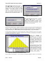
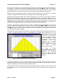
We are now ready to look at our first statistical distribution that is practical to use in contingency analysis.
This distribution is called the Triangular Distribution. Figure T1c will give you a clue as to why it is called
Part 2 - Tutorials
Page 19