Download Chapter 8, Thermal Conductivity

8. THERMAL CONDUCTIVITY
8.1. Principles
PHYS I C A L B A CK G ROU N D
The coefficient of thermal conductivity, k [W/(m·K)], is a measure of the rate q
(W) at which heat flows through a material. It is the coefficient of heat transfer
across a steady-state temperature difference (T2 – T1) over a distance (x2 – x1), or
q = k (∆T/∆x).
(1)
Thermal conductivity can be measured by transient heating of a material with a
known heating power generated from a source of known geometry and measuring
the temperature change with time. The method assumes isotropic materials.
Theoretical discussion for measuring thermal conductivity with cylindrical sources
is found in Blackwell (1954), Carslaw and Jaeger (1959), De Vries et al. (1958),
Von Herzen and Maxwell (1959), Kristiansen (1982), and Vacquier (1985).
For a full-space needle probe, the length L can be assumed to be infinite and the
problem is reduced to two dimensions. Given the resistance R of a looped wire in a
needle, the generated heat is
q = 2 i2 R / L,
(2)
where R/L is the resistance of the needle per unit length. At any time t after heating
has started, the temperature T is related to the thermal conductivity k by
T = (q / 4πk) ln(t) + C,
(3)
where q is the heat input per unit length and unit time and C is a constant. A simple
way of calculating the thermal conductivity coefficient k is picking T1 and T2 at
times t1 and t2, respectively, from the temperature versus time measurement curve
(see also ASTM, 1993):
ka(t) = q / 4π [ln(t2) - ln(t1)] / (T2 - T1).
(4)
ka(t) is the apparent thermal conductivity because the true conductivity, k, is
approached only by a sufficiently large heating duration. This method assumes that
the measurement curve is linear and ignores the imperfections of the experiment
expressed in the constant C.
In practice, the correct choice of a time interval is difficult. During the early stage
of heating, the source temperature is affected by the contact resistance between the
source and the surrounding material. During the later stage of heating, boundary
effects of the finite length of the source affect the measurement. The position of the
optimum interval generally differs from measurement to measurement. The two
systems presently available on the ship employ different procedures to select the
time interval: the older Thermcon-85 system relies on operator judgment based on
visual examination of the ln(t) vs. T plot; the newer TK04 system uses an
PP Handbook , Peter Blum , November, 1997
8—1
algorithm that automatically finds the optimal time interval (Erbas, 1985). More
information is provided about each in the following sections.
EN VIRONMENTAL EFFECTS
In situ thermal conductivity is a function of in situ temperature and pressure
conditions. Corrections may be applied to laboratory measurements on cores,
based on in situ information and theoretical and empirical relationships. Data in
the ODP database are not corrected for in situ conditions.
USE OF THERMAL CONDUC TIVITY
Thermal conductivity is an intrinsic material property for which the values depend
on the chemical composition, porosity, density, structure, and fabric of the material
(e.g., Jumikis, 1966). In marine geophysics, mainly thermal conductivity profiles
of sediment and rock sections are used, along with temperature measurements, to
determine heat flow. Heat flow is not only characteristic of the material, but an
indicator of type and age of ocean crust and fluid circulation processes at shallow
and great depths.
8.2. Thermcon-85 System
EQ U I P ME N T
The Thermcon-85 system consists of the following components:
• Thermcon-85 unit,
• calibrated needle probes,
• personal computer,
• TC-PC control and data reduction program, and
• calibration file for TC-PC.
The Thermcon-85 unit was purchased from Woods Hole Oceanographic
Institution. It is under the control of PROM-based programming, and an RS-232
serial interface is available. One to five needle probes can be connected to the rear
panel. An eight-channel multiplexer selects the appropriate input for each
measurement. See the Thermcon-85 manual for more details.
The needle probes are either assembled at ODP or purchased preassembled. In
either case, they contain factory-calibrated thermistors.
The TC-PC program was developed at ODP in 1991 using Quick Basic (v. 4.5) and
runs on a PC clone. The following programs are involved:
• TCMENU: controls the overall data acquisition process;
• COLLECT: communicates with the Thermcon-85; performs drift study;
collects raw data and writes raw data file; monitors “bad data conditions”
(warnings not written to data file);
8—2
PP Handbook , Peter Blum , November, 1997
• PROCESS: allows selection of probe positions; allows for optional
correction for temperature drift at drift study termination; allows selection
of “optimal” interval; reduces the raw data and calculates thermal
conductivity; writes to a results file; and
• PROBES: used to enter thermistor calibration coefficients for new probes
and “secondary” probe calibration constants into the PROBES.DAT file.
The user normally runs TCMENU. Interaction with the COLLECT and PROCESS
programs is accomplished via menu selection. The calibration data must be entered
into the PROBES.DAT file when appropriate.
CALIBRAT IO N
Power Supply, Digital
Volt Meter, and
Heater Current
Calibration must be periodically performed by an ODP Electronics Technician.
Refer to the Thermcon-85 manual for details.
Needle Probe
Resistance
The thermistors in each needle probe are calibrated at the factory over a range of
temperatures (usually 15° to 75°C) and fit to an equation of the form
T-1 = alpha + beta ln(R) + gamma (ln(R))3,
(5)
where T is the temperature in degrees Kelvin, R is the thermistor resistance in
ohms, and alpha, beta, and gamma are constants. The error in this procedure is far
smaller than the general uncertainty in thermal conductivity measurements. The
constants are available to the data reduction program and are used for conversion
of measured resistance into temperature. Electronics Technicians are responsible
for entering the constants of a new resistor into the program. Do not attempt to recalibrate the thermistors—a specialized facility is required.
Needle Probe
Secondary
Calibration
ODP procedure with the Thermcon-85 system includes a calibration of each
needle probe using standard materials of “known” thermal conductivity values
(Table 8—1). These values were established on Legs 127, 129, and 131 and on
subsequent legs using this same instrument. This calibration should be viewed as a
relative one that makes ODP shipboard data a little more consistent.
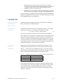
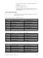
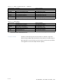
Table 8—1
Standard materials used for calibrations and control measurements.
Standard material
Thermal conductivity [W/(m·K)]
Black rubber
0.54
Red rubber
0.96
Macor
1.61
The standard measurements must be entered into a separate spreadsheet and the
liner coefficients (slope, intercept) determined. The coefficients are then entered
into the PROBES.DAT file using the PROBES program utility. The thermal
conductivity values returned by the PC-TC program are subsequently corrected
using these coefficients.
PP Handbook , Peter Blum , November, 1997
8—3
PERFORM ANCE
Precision
About 5%. (Systematic evaluation is required.)
Accuracy
About 5%. (Systematic evaluation is required.)
MEASUREMEN T
1. Bring cores to temperature equilibrium (about 4 hr). Hard-rock specimens
should be placed in a water bath to equilibrate.
2. Soft sediment: drill holes into core liner. Also drill a small hole in
semiconsolidated sediment if necessary. Apply thermal joint compound if
necessary. Insert full-space probes carefully into sediment. Rocks: prepare
smooth surface on a split-core specimen at least 5 cm long. Treat the
needles gently, and store them properly when not in use.
3. Insert one probe into a standard material for a control measurement, to be
used for later corrections if necessary.
4. Start the TCMENU program and follow the prompts for parameters.
Default values are provided for each prompt.
5. Press the reset button on the Thermcon-85 unit to start the drift study. After
a couple of minutes, the drift data will be displayed. The drift study is
performed in phases of 25 minutes, the maximum time the box can be
programmed. The drift study is terminated if all positions are equilibrated or
if the user overrides the drift study.
6. Press the reset button twice to start the process of heating, data acquisition,
and creation of the raw data file. Messages will be displayed if there are
data or hardware problems.
7. The user has the option of acquiring more data and processing batches of
data later or processing the data collected immediately. It is recommended
to process the data immediately.
8. Load the PROCESS program from the TCMENU screen. The run just
completed will appear as the default run to be processed. Accept or change
it.
9. Select the position to be processed and the drift correction. The ln(t) vs. T
graph will be displayed.
10. Select the time interval to be processed by moving the cross hairs on the
screen. For routine processing, use the same interval used for secondary
probe calibration. Adjust if necessary. Press enter to calculate conductivity
and the fit parameter. Warnings will come up if the nonlinear component is
considered too large, the fit is poor, the segment is considered too short, etc.
11. Press enter twice to write the conductivity of a segment to the Results file.
DATA PROCESSING
Data reduction with the TC-PC program written for the Thermcon-85 system is
based on a least-squares fit of the measured temperatures to the following
equation, which is a variation of Equation XXX(107?):
T = (q / 4¼k) ln(t) + At + B.
(6)
8—4
PP Handbook , Peter Blum , November, 1997
The constant A is the temperature drift rate (also including edge effect, asymmetry,
nonzero epoxy conductivity, etc.) during measurement and is expressed in K/min.
The constant B represents other imperfections in the experiment. The unknowns in
this system are k, A, and B, so when more than three data pairs are acquired the
system is overdetermined. Using the previous equation for the rate of heating, the
coefficient k can be determined at any time increment dt as
k = [2 i2 R / L dln(t)] / 4¼ (dT - At - B)], or
2
k = (i R / 2¼L) [dln(t) / (dT)].
(7)
(8)
The first group of terms in these equations is an instrument constant including
generated heat and needle geometry. The second group of terms is calculated for
each measurement.
The optimum time segment for calculating thermal conductivity is selected
interactively by the user by placing cross hairs on a ln(t) vs. T plot of the data.
Information on the quality of the fit is updated on the screen as the cross-hairs are
moved. The curve-fit parameter is the root mean square of the temperature
deviation and should not exceed 0.04°C/min. However, it is more important to
choose a consistent sampling time than it is to reduce the drift as much as possible.
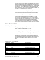
DATA SPECIFICATIONS
TC-PC Output Files
At present, the TC-PC data are not integrated in the new ODP database. The
following two program output files are archived: the “Processed Data” or
“Results” (*.DAT) files and the “Raw Data” (*.TC) files.
Data in the *.DAT files are fixed format, mixed string, and numeric, with one
record (line) per position per TC run. If a given position on a run is not processed,
then there is no entry in this file. However, if a given position is processed more
than once, there are multiple lines in this file for that position. The file name is the
hole identifier.
Data in the *.RAW files are free-format in which each line represents an output
string from the program. If a position was not used, some strings are omitted and
some return zero values. The file name is a combination of hole ID and run
number.
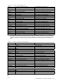
Table 8—2
TC-PC “Processed Data” file.
Short description
Leg
Site
Hole
Core
Core type
Section
Top
Bottom
Space
Run No.
Probe
Position
TC uncorr.
Description
Leg
Site
Hole
Core
Core type
Section
Interval top (cm)
Interval bottom (cm)
Space model
Run number
Probe number
Position number
Uncorr. thermal conductivity. [W/(m·K)]
PP Handbook , Peter Blum , November, 1997
Data file designations
[TC-PC Results 1-4] leg
[TC-PC Results 8-11] site
[TC-PC Results 13] hole
[TC-PC Results 15-17] core
[TC-PC Results 19] core_type
[TC-PC Results 21-22] section_or_std
[TC-PC Results 24-28] interval_top
[TC-PC Results 30-34] interval_bottom
[TC-PC Results 49] full_or_half
[TC-PC Results 51-53] run_number
[TC-PC Results 55-57] probe_number
[TC-PC Results 59] position_number
[TC-PC Results 61-67] calculated_tc
8—5
Table 8—2
TC corr.
R2
Drift
Lower end
First time
Upper end
Last time
Drift status
T drift
Drift rate
Drift fit
Run status
Alpha
Beta
Gamma
Resistance
Half space
Probe m1
Probe m0
Lower end
Upper end
Drift corr.
Version
Comment
TC-PC “Processed Data” file.
Corr. thermal conductivity. [W/(m·K)]
2
Standard error R
Calculated drift (°C/s)
Lower end point used
Time at lower end point (s)
Upper end point used
Time at upper end point (s)
Drift study status
Temp. at drift study termination (°C)
Drift rate at termination (°C/s)
Least-squares fit for drift
Run status (NORMAL, ...)
Probe alpha constant
Probe beta constant
Probe gamma constant
Probe wire resistance (ohm/cm)
Probe half-space flag (1 = true)
Probe secondary calibration slope
Probe secondary calibration intercept
Upper end point, probe calibration (s)
Lower end point, probe calibration (s)
Drift correction status
Version of TC-PC program
Comment
[TC-PC Results 69-75] corrected_tc
[TC-PC Results 77-87] standard_error
[TC-PC Results 89-97] calculated_drift
[TC-PC Results 99-100] lower_end_point
[TC-PC Results 102-104] time_at_first_point
[TC-PC Results 106-107] upper_end_point
[TC-PC Results 109-111] time_at_last_point
[TC-PC Results 113-126] drift_status
[TC-PC Results 128-132] drift_temperature
[TC-PC Results 134-142] drift_rate
[TC-PC Results 144-151] drift_fit
[TC-PC Results 153-160] run_status
[TC-PC Results 162-180] probe_alpha
[TC-PC Results 182-200] probe_beta
[TC-PC Results 202-220] probe_gamma
[TC-PC Results 222-227] probe_wire_resistance
[TC-PC Results 229-230] half_space_flag
[TC-PC Results 232=238] probe_m1
[TC-PC Results 240-246] probe_m0
[TC-PC Results 248-250] time_at_first_point
[TC-PC Results 252-254] time_at_last_point
[TC-PC Results 256-268] drift_correction_status
[TC-PC Results 270-274] tcpc_version
[TC-PC Results 276-356] comment
Notes: The numbers following the file name (TC-PC Results . . .) are positions in the fixed-space format of the output file.
Corrected thermal conductivity is corrected using the secondary probe calibration coefficients m1 and m0 obtained from
standard measurements. Corrected thermal conductivity is added only if the user selects this option when specifying data
reduction. If correction is not selected, the position numbers are reduced by 8 spaces starting with the “Standard error”
field.
Table 8—3
TC-PC “Raw Data” file (free format).
Short description Description
Run parameters
Title
Title string
Run
Run number
Positions
No. of positions used; length (min.)
Parameters for first position
Sample ID
ODP sample identification
Piece
Piece
Subpiece
Subpiece
Space
Space model
Position no.
Position number
Alpha
Probe alpha constant
Beta
Probe beta constant
Gamma
Probe gamma constant
Resistance
Probe wire resistance (ohm/cm)
Half space
Probe half-space flag (1 = half)
Probe secondary calibr. slope
Probe m1
Data file designations
[TC-PC Raw 1] title
[TC-PC Raw 2] run_number
[TC-PC Raw 3] no_of_positions_length
[TC-PC Raw 4] sample_id
[TC-PC Raw 5] piece
[TC-PC Raw 5] sub_piece
[TC-PC Raw 7] full_or_half
[TC-PC Raw 8] position_number
[TC-PC Raw 9.1] probe_alpha
[TC-PC Raw 9.2] probe_beta
[TC-PC Raw 9.3] probe_gamma
[TC-PC Raw 9.4] probe_wire_resistance
[TC-PC Raw 9.5] half_space_flag
[TC-PC Raw 9.6] probe_m1
Probe m0
Probe secondary calibr. intercept
[TC-PC Raw 9.7] probe_m0
Lower end
Upper end
Comment
Lower end point, probe calib. (s)
Upper end point, probe calib. (s)
Position-specific comment
[TC-PC Raw 9.8] time_at_first_point
[TC-PC Raw 9.9] time_at_last_point
[TC-PC Raw 10] comment
Parameters repeated for other positionsa
Drift time
Drift: no. of readings; length(s)
Drift study for first position
Drift t-T
String of time-temperature pairs
Drift end
Temp., rate., fit, at end of drift study
[TC-PC Raw one line, two values]
[TC-PC Raw one line, unlimited pairs]
[TC-PC Raw one line, three values]
Drift study repeated for other positionsb
8—6
PP Handbook , Peter Blum , November, 1997
Table 8—3
TC-PC “Raw Data” file (free format).
Drift status
Drift status (OK; OVERRIDE)
Data for positions 1–5
Data
Cycle #; ref. volt; I1 to I5; current
[TC-PC Raw one line, one alpha string]
[TC-PC Raw multiple lines, 3-8 values per line)
Data repeated for each meas. cyclec
Run status
Run status (NORMAL...)
[TC-PC Raw one line, one alpha string]
aThe
Notes:
probe parameters of lines 4–10 are written for subsequent positions only if the positions were used, otherwise
the lines are omitted. bThe drift study data lines (two lines per position) are always written to the file regardless whether
positions were used or not. If a position was not used, all values are zero. cData are written on one line for each
measurement cycle. On each line, there are the following readings separated in time by 3 s (hard-coded in the program):
(1) cycle number; (2) internal reference voltage; (3) to (7) up to five probe voltage readings (no reading for unused
positions); (8) heater current. Total time for one cycle is (2 + <number of positions used>) times 3 s (2 stands for reference
and heater current readings). It varies between 6 s (no position used) and 21 s (five positions used).
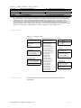
Database Model
Table 8—4
Database model
TCON section
tcon_id [PK1] [FK]
tcon_probe_num [PK2] [FK]
top_interval
bottom_interval
section_id
TCON control
tcon_id [PK1] [FK]
tcon_probe_num [PK2] [FK]
standard_id [PK3] [FK]
TCON drift raw data
tcon_id [PK1] [FK]
tcon_probe_num [PK2] [FK]
tcon_raw_drift_time [PK3]
tcon_raw_drift_temp
Standard Queries
TCON probe proc. data
tcon_id [PK1] [FK]
tcon_probe_num [PK2]
tcon_comment
tcon_meas_calib_m0
tcon_meas_calib_m1
tcon_meas_calib_time_first
tcon_meas_calib_time_last
tcon_meas_drift_lsq_fit
tcon_meas_drift_rate_final
tcon_meas_drift_temp_final
tcon_probe_alpha
tcon_probe_beta
tcon_probe_gamma
tcon_probe_half_full
tcon_probe_specific_res
tcon_proc_drift_corr_flag
tcon_proc_point_first
tcon_proc_point_last
tcon_proc_thermcon
tcon_proc_time_first
tcon_proc_time_last
tcon_raw_drift_status
tcon_raw_pos_num
TCON run
tcon_id [PK1]
tcon_run_minutes
tcon_run_number
tcon_run_status
TCON cycle
tcon_id [PK1] [FK]
tcon_cycle_num [PK2]
tcon_raw_heater_current
tcon_raw_heater_curr_time
tcon_raw_rel_voltage
tcon_raw_rel_voltage_time
TCON probe cycle
tcon_id [PK1] [FK]
tcon_cycle_num [PK2] [FK]
tcon_probe_num [PK3]
tcon_raw_time
tcon_raw_voltage
The standard queries will be defined once the upload routine has been
implemented.
PP Handbook , Peter Blum , November, 1997
8—7
8.3. TK04 System
EQ U I P ME N T
ODP purchased the TK04 system in late 1995 and deployed it permanently on the
ship on Leg 168 (1996). The system was to replace the ailing Thermcon-85 device,
built at the Woods Hole Oceanographic Institution (WHOI) and in service on the
ship for many years. Currently, both systems are available to the user on the ship.
The TK04 was built by the Berlin company Teka based on an apparatus that had
been developed at the Technische Universität Berlin. It was used successfully for
thousands of measurements on material from the Continental Deep Drilling
Program (KTB). The TK04 consists of
• automatic self-test, heating, and measurement unit TK04,
• full-space (VLQ) and half-space (HLQ) needle probes,
• vice and manual hydraulic pump for half-space contact measurements on
rocks, and
• Macor standards for both types of needle probes.
The TK04 measuring system features a self-test at the beginning of each
measuring cycle (including probe number validation), registration of the source
temperature and its drift, and calculation of the heating power used.
The following executable programs are used to operate the system:
• TKMEAS.EXE to acquire time-temperature data series (creating *.DWL
files),
• TKEVA for standard (<5% uncertainty) or special (<2% uncertainty) reevaluation of data, creating short *.DAT or long *.ERG lists and
parameter files, and
• TKGRAPH to display all solutions and assess the quality of the
calculated solutions.
In addition, the following parameter files are used:
• TKMEAS.MNU, a list of standard menu settings for TKMEAS.EXE,
• *.INI, list of parameters for probes, where “*” is the number engraved on
the probe, and
• TKEVA.INI, list of user-modifiable parameters required for
TKEVA.EXE.
Multiple measurements can be taken under identical conditions. The instrument
cycles through the measurements automatically, creating files with the userdefined root name (e.g., Core-Section-Interval; only six characters allowed) and a
two-digit serial number incrementing by one for each measurement within a cycle.
The following files are created by the TK04 system:
• <Rootname-SerialNo>.DWL, (if “Save data” was selected); contains
measurement parameters and temperature-time series (raw data), required
for extended evaluations; it is not necessary, but strongly recommended,
to save the heating curves for routine evaluation. These files allow later
extended evaluation and graphical display of the solutions.
• <Rootname->.LST, short list of results from evaluating one root-namebatch of *.DWL files using either the “special approximation method”
8—8
PP Handbook , Peter Blum , November, 1997
(SAM) or conventional (CON) method; contains evaluation parameters
and the optimal calculated thermal conductivity value. This is the
standard results file.
• TC-LIST.DAT, multiline short list (optional); contains the same
information as previous file <Rootname->.LST but for multiple root
names. This file is updated as new evaluations are performed. This file is
created only by the optional extended evaluation.
• <Rootname>.ERG, long lists of results from evaluating *.DWL files with
the SAM method; contains evaluation parameters and all valid calculated
thermal conductivity values. This file is optional and required only if
graphical evaluation of all valid solutions is desired. It can be created at
any time if the *.DWL files are saved. This file is created only by the
optional extended evaluation.
CALIBRAT IO N
No calibration is required. The unit conducts a self-test at the beginning of each
measurement cycle. Macor standards are used to confirm the 1.65 W/(m·K) value.
DATA PROCESSING
The Special
Approximation
Method (SAM)
The main advantage of the Teka data reduction program is the SAM that ensures
that only results of physical significance are considered. The critical choice of time
interval for calculation of conductivity, selected manually by the user with the
Thermcon-85 system, is accomplished by an algorithm that automatically finds the
optimal time interval. The solution can be judged in great detail and the data
reevaluated with different boundary parameters if warranted. The following
explanations are modified from the Teka user manual.
The first evaluation step is an approximation to the solution of a constantly heated
line source (Kristiansen, 1982):
(9)
T(t) = A1 + A2ln(t) + A3[ln(t)/t] + A4(1/t).
The coefficients Ai are calculated with the least-squares method. A1, A3, and A4 are
related to source geometry and thermal properties. A2 is calculated by
A2 = q / 4πk,
(10)
where q is the heating power (Wm) and k [W/(m·K)] is the thermal conductivity. If
the coefficients Ai are determined, T(t) can be expressed analytically and the
apparent thermal conductivity Ka(t) can be calculated by differentiating Equation
on page 9 with respect to ln(t):
ka(t) = dT/dln(t) = q/4π {A2 + A3[1/t – ln(t)/t] + A4/t}.
(11)
It can be shown that the desired value k is at ka(tmax), where tmax is the “extreme
time.” The requirement for the maximum is
d/dt[ka(tmax)] = 0,
(12)
and tmax is
tmax = e(2A3–A4)/A3, A3 > 0.
(13)
The logarithm of the extreme time (LET) becomes
PP Handbook , Peter Blum , November, 1997
8—9
LET = ln(tmax) = (2A3 - A4) / A3.
The time-dependent terms in previous equation are:
T(tmax) = A2ln(tmax) + A3[ln(tmax)/tmax] + A4/tmax.
(14)
(15)
A4 can be substituted with (previous) Equation (118?) to give
T(tmax) = A2ln(tmax) + 2A3[ln(tmax)/tmax].
(16)
This equation shows that the purely logarithmic dependence of the approximated
temperature (required by the theory) is stronger the larger tmax gets. For large tmax,
the second term in Equation on page 10 approaches zero.
The evaluation procedure approximates the heating curve in as many time
intervals as possible and examines each interval for its suitability for thermal
conductivity calculation using the following criteria:
1. ka(t) is located above a given value of time defined by LET,
2. standard deviation of the function for A2 is below a given value,
3. ka(t) is a maximum: A3 > 0, and
4. derivation ka(t) is continuous for t = tmax: A2tmax – A3 - 0.
If these criteria are met, thermal conductivity can be calculated as
k = q / (4πA2).
(17)
The evaluation interval is restricted by the dimension of the line source. It must be
within the interval of 20 to 80 s to avoid boundary effects, and at least 25 s long for
a stable calculation of the coefficients. The input parameters for standard
evaluation are
• minimum duration of approximation interval: 25 s,
• start of first approximation interval: 20 s,
• end of last approximation interval: 80 s,
• lower limit for LET: 4, and
• maximum standard deviation of calculated temperature curve from
measured heating curve: 0.0003.
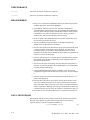
With the default parameters, the heating curve is approximated for the following
time intervals:
[20,45] [20,46] [20,47] . . . [20,78] [20,79] [20,80]
[21,46] [21,47] . . . [21,78] [21,79] [21,80]
[22,47] . . . [22,78] [22,79] [22,80]
...
[53,78] [53,79] [53,80]
[54,79] [54,80]
[55,80]
Among all time intervals that fulfill the listed criteria, the one with the largest LET
is used to calculate thermal conductivity. No solutions may be found if the
measurement is disturbed by poor sample condition or ambient temperature
changes.
Extended Evaluation
8—10
An extended evaluation is required if
PP Handbook , Peter Blum , November, 1997
• the valid solutions are to be plotted against the calculation parameters to
judge the results graphically, or
• the measurements are to be reevaluated with different parameters (e.g., a
stronger criterion for the LET).
In both cases, the *.DWL files containing the temperature-time data are required.
The *.ERG files (long result lists) that can be created contain all valid solutions for
the thermal conductivity, and a line entry in the TC-LIST.DAT file is created with
the asymptotic (optimal) thermal conductivity value. There are three options for
extended evaluation:
• single evaluation: typing <TKSAM> prompts for filename,
• batch mode with filename as parameter: typing <TKSAM filename>
starts evaluation using the standard parameters (no *.ERG file is created),
and
• Batch mode evaluating a sequence of data files: after typing TKSAM,
type return instead of a filename; all *.DWL files in the directory will be
evaluated.
The manufacturer’s manual should be consulted for details in regard to file path
requirements, data quality issues, etc.
Graphical Evaluation
The program TKGRAPH can be used to visualize and judge the quality of all valid
SAM evaluation results for thermal conductivity. *.ERG files are required for
plotting. Four graphs are presented for each measurement:
• thermal conductivity vs. LET,
• thermal conductivity vs. interval duration,
• thermal conductivity vs. start of interval, and
• thermal conductivity vs. end of interval.
A series of files can also be viewed. Consult the manufacturer’s manual for system
configuration, practical hints, guidance for the judgment of results, etc.
Evaluation with
Conventional Method
Under certain experimental circumstances (e.g., porous material, high water
content) the SAM evaluation may not accept any results because the
measurements are too disturbed for the sensitive approximations. In these cases,
results may be obtained using the conventional evaluation method in which
thermal conductivity is calculated from the inverse slope of the heating curve in a
section of logarithmic linearity. In general, a heating duration > 80 s becomes
necessary. Accuracy of conventional evaluations is not as good as that of SAM
evaluations and the quality cannot be verified graphically.
The program TKCON.EXE is used for the conventional evaluation. The structure
and application is similar to the TKSAM.EXE program. The configuration file
TKCON.INI includes the following standard parameters:
• minimum duration of interval: 30 s,
• start time:
30 s,
• end time:
120 s, and
• standard deviation of fit: 0.003.
PP Handbook , Peter Blum , November, 1997
8—11
Existing data can be evaluated later with the conventional method (i.e., after the
SAM method has failed to yield solutions). Automatic Evaluation with TKCON
can be set by typing
TKMEAS/EVA=CON
or if the option
TKMEAS/DCL=20/EVA=CON
is entered. Calling TKMEAS without the /EVA option invokes evaluation with
TKSAM.EXE.
A short list of results is created by TKCON with similar structure as the file
created by TKSAM. The difference is that instead of LET the standard deviation is
reported. The evaluation method used (SAM; CON) is indicated in each line of the
file. A long list of results for each measurement can be produced by typing, prior
to starting TKMEAS:
set TKCON=ON
The long list includes the calculated values of thermal conductivity, standard
deviation, and the start, duration, and end of each interval.
Half-Space
Measurements
For the half-space needle probe (HLQ) it is expected that the total amount of
produced heat penetrates into the sample. The thermal conductivity is thus
calculated with twice the heating power used for the full-space solution. This
assumption is justified if the thermal conductivity of the samples is not lower than
about 1 W/(m·K); at lower values an error arises because some of the produced
heat is penetrating the probe half-space, in which case it is necessary to determine
correction factors to compensate for the heat loss.
PERFORM ANCE
Precision
Extended evaluation, using special parameters adapted to circumstances, yields an
uncertainty of less than 2%. This is clearly smaller than variations caused by
sample preparation and inhomogeneities in rocks and sediments, and special
evaluations are appropriate only for standard materials and fundamental material
investigations.
Accuracy
Random variations of thermal conductivity in natural materials such as sediments
and rocks typically give an uncertainty of about 5%. Routine evaluation using the
TKEVA.EXE has an accuracy of about 5% and is therefore appropriate.
MEASUREMEN T
Standard Settings for
Data Acquisition
1. Bring cores to temperature equilibrium (about 4 hr). Hard-rock specimens
should be placed in a water bath to equilibrate.
2. Soft sediment: drill holes into core liner. Also drill a small hole in
semiconsolidated sediment if necessary. Apply thermal joint compound if
necessary. Insert full-space probes carefully into sediment. Hard-rocks:
prepare smooth surface on a half-core specimen at least 5 cm long. Treat
needles gently, store them properly when not in use.
8—12
PP Handbook , Peter Blum , November, 1997
3. On the computer, change to directory containing the TKMEAS.EXE file,
press enter.
4. Type TKERG = ON, press enter.
5. Type the command tkmeas, press enter.
6. Set the parameters on the screen. Heating power should be about 5 W/m
(adjust if necessary); measuring time should be about 80 s; enter Y to save
time-temperature data.
DATA SPECIFICATIONS
TK04 Output Files
Table 8—5
TK04 “raw data file”: <Rootname-Serial>.DWL.
Short description
Header
Filename
Probe
Comment
Heat
Fit
?Something
?Value1
?Value2
Data
Temp
Time
Resistance
Table 8—6
Description
Data file designation
Root name (custom sample id), serial
Probe ID, TK04, date
Comment, used to identify sample
Heating power (W/m)
Slope, Std. dev., temperature
?’Reserved’
?Some (drift?) value 1
?Some (drift?) value 2
[TK04 Raw Data] rootname_serial
[TK04 Raw Data] probe
[TK04 Raw Data] comment
[TK04 Raw Data] heating_power
[TK04 Raw Data] fit
[TK04 Raw Data] ?something
[TK04 Raw Data] ?value1
[TK04 Raw Data] ?value2
Temperature (°C)
Time (s)
Resistance (ohm)
[TK04 Raw Data] temperature
[TK04 Raw Data] time
[TK04 Raw Data] resistance
TK04 “results short list”: <Rootname>.LST (one rootname batch).
Short description
Filename
TC
LET/STD
Solutions
Start time
Time
End time
Eval.
Hints
Table 8—7
Currently, TK04 data are not integrated in the new ODP database. The following
program output files are archived.
Description
Root name + serial (sample ID)
Calculated thermal conductivity
LET (SAM) of std. dev. (CON)
No. of solutions found
Start of approx. time interval (s)
Length of approx. time interval (s)
End of optimal time interval (s)
Evaluation method (SAM or CON)
Comments (from *.DWL file)
Data file designation
[TK04 Results] rootname_serial
[TK04 Results] calculated_tc
[TK04 Results] let_or_sd
[TK04 Results] solutions
[TK04 Results] time_start
[TK04 Results] time_length
[TK04 Results] time_end
[TK04 Results] eval_method
[TK04 Results] hints
*TK04 “appended results short list”: <Rootname>.LST (all rootnames).
Short description
Filename
TC
LET/STD
Solutions
Start time
Time
End time
Eval.
Hints
Description
Root name + serial (sample id)
Calculated thermal conductivity
LET (SAM) of std. dev. (CON)
Number of solutions found
Start of approximate time interval (s)
Length of approx. time interval (s)
End of optimal time interval (s)
Evaluation method (SAM or CON)
Comments (from *.DWL file)
PP Handbook , Peter Blum , November, 1997
Data file designation
[TK04 Results] rootname_serial
[TK04 Results] calculated_tc
[TK04 Results] let_or_sd
[TK04 Results] solutions
[TK04 Results] time_start
[TK04 Results] time_length
[TK04 Results] time_end
[TK04 Results] eval_method
[TK04 Results] hints
8—13
Table 8—8
*TK04 “extended results file”: *.ERG files.
Short description
Header:
Filename
Comment
Time
Start time
End time
LET
Std. Dev.
Table 8—9
Description
SAM Evaluation Parameters
Root name + serial (sample ID)
Comment, used to identify sample
Time interval minimum (s)
Start of evaluation (s)
End of optimal time interval (s)
Nat. log. of time
Limit of std. dev. (optional; 0.0003)
Data file designation
TKSAM.EXE
[TK04 Results] rootname_serial
[TK04 Raw Data] comment
[TK04 Results] eval_interval_min
[TK04 Results] eval_time_start
[TK04 Results] eval_time_end
[TK04 Results] eval_let
[TK04 Results] eval_limit_sd
Valid solutions.
Short description
TC
LET
Start time
Time
End time
Std. Dev.
Description
Calculated thermal conductivity
Natural logarithm of time at max. therm.al condition
Start of approx. time interval (s)
Length of approx. time interval (s)
End of optimal time interval (s)
Standard deviation of fit
Data file designation
[TK04 Results] calculated_tc
[TK04 Results] let
[TK04 Results] time_start
[TK04 Results] time_length
[TK04 Results] time_end
[TK04 Results] std-deviation
Notes: *ERG files are optional. They are created by extended evaluation and are required only for graphical evaluation. They
can be recreated from *.DWL files at any time.
Database Model
8—14
A database model and integration into the database are difficult to implement
without writing an ODP sample identification routine linked to the TK04 output. A
better approach is to write an entirely new user interface for the system, preferably
for an upgraded version with multiple-channel capability.
PP Handbook , Peter Blum , November, 1997