Download DoubletCalc v143 manual english

Oil and Gas
Princetonlaan 6
3584 CB Utrecht
P.O. Box 80015
3508 TA Utrecht
The Netherlands
TNO report
www.tno.nl
TNO 2014 R11396
DoubletCalc 1.4 manual
English version for DoubletCalc 1.4.3
Date
1 October 2014
Author(s)
H.F. Mijnlieff, A.N.M. Obdam, J.D.A.M. van Wees, M.P.D.
Pluymaekers and J.G. Veldkamp
Copy no
No. of copies
Number of pages
Number of
appendices
Sponsor
Project name
Project number
54 (incl. appendices)
All rights reserved.
No part of this publication may be reproduced and/or published by print, photoprint,
microfilm or any other means without the previous written consent of TNO.
In case this report was drafted on instructions, the rights and obligations of contracting
parties are subject to either the General Terms and Conditions for commissions to TNO, or
the relevant agreement concluded between the contracting parties. Submitting the report for
inspection to parties who have a direct interest is permitted.
© 2014 TNO
T +31 88 866 42 56
F +31 88 866 44 75
TNO report | TNO 2014 R11396
2 / 45
Contents
1
Introduction .............................................................................................................. 5
2
2.1
2.2
2.3
2.4
User manual DoubletCalc v1.4 ............................................................................... 6
Installation of the software ......................................................................................... 6
Input screen ............................................................................................................... 7
Output screen .......................................................................................................... 10
Error messages ....................................................................................................... 15
3
3.1
3.2
The DoubletCalc model ......................................................................................... 18
Remarks regarding the model ................................................................................. 19
Penetrating the aquifer obliquely ............................................................................. 20
4
Theoretical background of the DoubletCalc model ........................................... 23
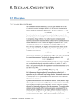
5
5.1
5.2
5.3
5.4
5.5
5.6
5.7
Mass balance ......................................................................................................... 26
Mass flow ................................................................................................................. 26
Volume flow ............................................................................................................. 26
Impulse balance....................................................................................................... 26
Pressure development in the aquifer from or towards a well .................................. 27
Pressure development in a casing .......................................................................... 28
Pressure development in the pump ......................................................................... 29
Initial hydrostatic aquifer pressure near the production and injection wells ............ 30
6
6.1
6.2
6.3
Energy balance ...................................................................................................... 31
Geothermal gradient ................................................................................................ 31
Heat loss in the production well ............................................................................... 31
Temperature decrease in the heat exchanger ........................................................ 32
7
7.1
7.2
7.3
7.4
Water properties .................................................................................................... 34
Density ..................................................................................................................... 34
Viscosity ................................................................................................................... 34
Heat capacity ........................................................................................................... 34
Salt content .............................................................................................................. 35
8
The effect of penetrating the reservoir obliquely ............................................... 36
9
Solution method .................................................................................................... 38
10
Parameter range .................................................................................................... 39
11
11.1
11.2
11.3
Calculated characteristics of the geothermal doublet system ......................... 40
Geothermal power ................................................................................................... 40
Required pump power ............................................................................................. 40
Coefficient of performance (COP) ........................................................................... 40
12
12.1
12.2
12.3
Considerations....................................................................................................... 41
Power gain by density difference between production and injection well ............... 41
Difference between produced and injected flow ...................................................... 41
Viscosity of the injected water ................................................................................. 42
TNO report | TNO 2014 R11396
3 / 45
12.4
Depleted reservoir and negative pressures ............................................................. 42
13
References ............................................................................................................. 44
14
Signature ................................................................................................................ 45
Appendices
A Example of the 'base case details' file
B Sub-layers in an aquifer
C Explanation of characters and symbols
TNO report | TNO 2014 R11396
4 / 45
TNO report | TNO 2014 R11396
1
5 / 45
Introduction
DoubletCalc v1.4.3 is a software tool that was developed by TNO. It enables to
calculate a pre-drill indicative geothermal power of a future geothermal doublet by
specifying the key reservoir parameters, the casing scheme and the pump details.
DoubletCalc v1.4 is the successor to DoubletCalc v1.3. The major difference with
respect to v1.3 is the possibility to specify the casing scheme of the production and
injection wells, and a minimum-median-maximum range for the expected salinity.
DoubletCalc v1.4.3 has largely the same functionality as DoubletCalc v1.4. Both the
output to screen and to file has been extended.
This document first explains how the software is used. Next, it describes the way in
which a doublet is modelled. Finally, the software implementation is substantiated,
including a description of all equations.
The software can be downloaded from:
http://www.nlog.nl/nl/geothermalEnergy/DoubletCalc.html
TNO report | TNO 2014 R11396
2
User manual DoubletCalc v1.4
2.1
Installation of the software
6 / 45
The
software
can
be
found
on
the
website
www.nlog.nl
(http://www.nlog.nl/nl/geothermalEnergy/DoubletCalc.html). It is distributed as a
compressed (ZIP) file. In order to use the program, the ZIP file needs to be
downloaded and saved on the computer. Next, the compressed files need to be
unpacked. The user can choose in which folder the files will be stored. In principle a
folder named DoubletCalc14 will be created (for example) in which the following
files are stored:
2.1.1
the release notes 'DoubletCalc143 release notes.txt'
the program files named ‘DoubletCalc-143-26092014.jar’.
the JavaFX ‘runtime’ folder
example file of a DoubletCalc scenario 'example.xml'
the windows executable ‘DoubletCalc_v1_4_3.exe’
the batch file 'start_doubletcalc.bat' as an alternative executable
the shell script ‘start_doubletcalc_osx.sh’ for executing on OS X/Linux
Installation on a Windows computer
Java version 6 or newer should be installed. In order to execute DoubletCalc:
double click ‘DoubletCalc_v1_4_3.exe’ in your favourite file manager.
Figure 1
Location of the DoubletCalc files as visible in the Windows default file manager. The
file to be executed is named DoubletCalc_v1_4_3.exe
If DoubletCalc does not start, the following check can be performed:
-
-
2.1.2
Was the correct version of Java installed (version 6 or newer). This information
can be verified on the website http://www.java.com/en/download/installed.jsp.
Java can be downloaded from http://www.java.com/en/download/manual.jsp
Alternatively execute the batch file 'start_doubletcalc.bat' in a command window
(run-> cmd.exe)
Installation on Apple computers
Follow the same instructions as for Windows computers, and execute the shell
script ‘start_doubletcalc_osx.sh’ from the terminal.
TNO report | TNO 2014 R11396
7 / 45
If DoubletCalc does not start, the following check can be performed:
-
2.2
Assign execute permission to the start script. This can be done in a terminal
window by entering: chmod u+x start_doubletcalc_osx.sh
Input screen
After the Java installation, the DoubletCalc 1.4.3 input screen appears (Figure 2).
The input screen enables the user to specify the essential parameters that are
required to calculate the geothermal power estimate. Only the white fields are
obligatory. The values in the grey fields are calculated by the software. The min and
max values of the aquifer tops are calculated as +/- 10% of the median value.
Excessive as this may seem, it also accounts for the uncertainty in the geothermal
gradient, which is not user specified. The number of simulation runs and the
'calculation length subdivision' (both in blue) can be entered if desired.
It was deliberately decided to leave as many fields as possible empty after start up,
with the exception of those values that in the Netherlands vary the least, like the
geothermal gradient and the surface temperature. This was done to prevent that
proposed default values that are unrepresentative for a scenario are used in that
scenario erroneously – the user is now forced to select representative values. Zerovalues of the optional parameters (between square brackets) are ignored.
The input screen enables to open an existing scenario ('Open scenario'). In the
'Open scenario' screen the XML-file containing the required scenario can be
selected (Figure 3). After opening, the parameters of this scenario are shown.
On the other hand, the user can also start by entering scenario parameters. Once
the parameters have been entered, the new scenario can be saved ('Save
scenario', Figure 4).
TNO report | TNO 2014 R11396
8 / 45
1
2
3
4
5
6
Figure 2
DoubletCalc 1.4.3 input screen (the boxed numbers refer to the text under the casing
scheme on the next page).
Figure 3
DoubletCalc Open Scenario screen.
Figure 4
DoubletCalc Save Scenario screen.
TNO report | TNO 2014 R11396
9 / 45
Casing schedule
In DoubletCalc 1.4.3 the casing scheme has to be specified, including the relevant
characteristics of the pipes (inner diameter and roughness), to the top of the
aquifer. The Along Hole (AH) and True Vertical Depth (TVD) depth must be
specified, according to the same surface reference level as the aquifer depth values
(in the Netherlands, NAP or Amsterdam Ordnance Level). Using these parameters,
the resistance encountered by the water while flowing through the casing can be
calculated. Figure 2, under 'C) Well Properties', shows the essential well input
parameters for DoubletCalc 1.4.3:
1. the outer diameter of the producer and injector in the reservoir section. This
diameter, specified as inches, determines the areal extent of the surface through
which water can enter the wellbore. This is the open hole diameter.
2. the inclination of the well trajectory in the aquifer (in degrees relative to the vertical). In combination with the reservoir gross thickness and net-to-gross ratio, this
determines the length of the production interval. DoubletCalc assumes that the
entire reservoir section is connected to the well.
3. the top and base of the casing / liner section measured in meters along hole
(mAH).
4. the top and base of the casing / liner section measured in meters vertically (true
vertical depth, or TVD).
5. the inner diameter of the casing / liner, per section (inch), through which the
water is produced.
6. the roughness of the casing (milli-inch). The roughness and inner diameter determine the resistance the water encounters when flowing.
Figure 5, which is the graphical representation of the well design in Figure 2, shows
which parameters should be entered. The part of the well inside the reservoir (solid
blue in the figure) should not be specified under 'C) Well Properties' if the well is
completed using a slotted screen and / or gravel pack in an open hole. In all cases,
the drill bit size should be entered as 'outer diameter producer / injector'. If the top
part of the casing is unperforated, this will result in extra resistance. This part of the
casing must be entered in the scheme.
The detail in the upper right of Figure 5 shows how water will flow towards the
perforated section in an inclined well. The area though which water can enter the
well is increased by the inclined path of the well through the aquifer. More
information can be found in paragraph 3.2 (Penetrating the aquifer) and chapter 8
(The effect of penetrating the reservoir obliquely).
The depth of the top of the aquifer is varied stochastically during calculation of the
geothermal power. Therefore the specified architecture of the casing, with a fixed
end depth, does not fit the top of the aquifer anymore. To deal with this problem,
DoubletCalc will extend or shorten the tubing segment with the largest diameter
accordingly.
For reasons of calculation accuracy, DoubletCalc will split the well into segments of
equal length during the simulation (the 'calculation length subdivision' under section
'C) Well Properties' in the input screen of Figure 2. A weighted average of the
properties is assigned to segments crossing a tubing section boundary (see the
'base case details' file in paragraph 2.3.3). It is advisable to choose the segment
length in accordance with the well design. A very small segment length increases
the calculation time, whereas a very large length decreases the calculation
accuracy.
TNO report | TNO 2014 R11396
Figure 5
10 / 45
Schematic casing design. The part of the casing located in the reservoir (solid blue)
should only be specified under specific circumstances.
The calculation of the geothermal power can be started when all parameters have
been entered (button 'Calculate!'). When finished the Doublet Calculator 1.4.3
Result Table (Figure 6) will appear.
2.3
Output screen
The output screen shows on the left hand side in the column 'Geotechnics (Input)'
the input parameters that were entered in the Input Screen and consequently used
during the calculation. The column 'Geotechnics (Output)' on the right hand side
shows the results of the calculation. The first block 'Monte Carlo cases' shows the
results of the stochastic simulation. The second block 'Base case' shows the results
of a calculation in which only the median values were used (in case a range was
specified).
TNO report | TNO 2014 R11396
Figure 6
11 / 45
DoubletCalc 1.4.3 output screen.
The output screen has three options for presenting the results in different ways:
-
probabilistic plots
fingerprinting
export of the 'base case' details
The detailed output is described in the following paragraphs.
2.3.1
Probabilistic plots
The button 'probabilistic plots' generates a new window graphically showing the
probability distribution of the pump volume flow. In the upper left corner of the
window there is an option to show similar graphs for the geothermal power and the
coefficient of performance (COP) (Figure 7). Choosing the button 'Export CSV file'
will export the graphs numerical data to a text file (Figure 8).
TNO report | TNO 2014 R11396
2.3.2
Figure 7
Probabilistic plots for pump volume, geothermal power and COP.
Figure 8
DoubletCalc 1.4.3 Export Fingerprint to file screen
12 / 45
Fingerprinting graph
Figure 9 shows the graph that is generated using the Fingerprinting button.
DoubletCalc will calculate the geothermal power (green curve), COP (purple), flow
rate (red) and the required pump energy (blue) for varying pump pressure
differences that are around the specified pump pressure difference. The calculation
of these graphs uses the median values from the input screen.
TNO report | TNO 2014 R11396
Figure 9
2.3.3
13 / 45
DoubletCalc Fingerprint graph.
Base case details
The button ‘export base case details’ in the output screen writes the following
information to a CSV-file:
-
-
hydrostatic aquifer properties at the producer and injector, calculated along the
well path per section (as specified in the 'calculation length subdivision'): pressure, temperature, salinity, density and viscosity (Table 1)
'base case' details at the producer and injector, calculated along the well path
per section (as specified in the 'calculation length subdivision') (Table 2)
'base case' pressure and temperature at a number of key doublet nodes (Table
3)
'base case' results calculated for the doublet as a whole (Table 4)
stochastic results (P90, P50 and P10) for a number of parameters calculated for
the doublet as a whole (Table 5).
Appendix 1 shows an example of the base case details file.
Table 1
parameter
unit
description
Z
m
top depth of calculation segment
P
bar
pressure
T
°C
temperature
S
ppm
salinity
density
kg/m³
density
viscosity
Pa.s
viscosity
Base case details file parts 1 and 2: initial hydrostatic aquifer properties at producer
and injector, calculated per section ('calculation length subdivision').
TNO report | TNO 2014 R11396
14 / 45
parameter
unit
description
iN
-
calculation length section number
segment
-
tubing section number
L
m
depth (along borehole)
Z
m
depth (true vertical)
angle
°
modelled inclination
inner diameter
Inch
casing inner diameter
roughness
milli-inch
absolute casing roughness
P
bar
pressure
T
°C
temperature
S
Ppm
salinity (Total Dissolved Solids, NaCl equivalent)
density
kg/m³
fluid density
viscosity
Pa s
fluid viscosity
Qvol
m³/h
volume flow
dPGrav
bar
pressure difference as a result of gravity operating
on the density of the water
dPVisc
bar
pressure difference as a result of varying viscosity
dPpump
bar
pressure difference as a result of pump (input
screen)
Table 2
Base case details file parts 3 and 4: parameters calculated per section ('calculation
length subdivision') for the production and injection well.
== DOUBLET NODES ==
node nr.
node name
1
Aquifer_Prod
255.08
89.28
static aquifer pressure and temperature near the producer
2
Aquifer/Prod_Bottom
241.30
89.28
bottomhole flowing pressure and
temperature at the producer
5&6
Prod_Top/Entry_HE
16.35
86.51
wellhead pressure and temperature at the producer
7&9
Exit_HE/Inj_Top
16.35
35.00
wellhead pressure and temperature at the injector
10
Inj_Bottom/Aquifer
276.99
35.99
bottomhole flowing pressure and
temperature at the injector
11
Aquifer_Inj
251.18
89.28
static aquifer pressure and temperature near the injector
Table 3
P (bar)
T (°C)
location
Base case details file part 5: pressure and temperature at specific locations in the
doublet schedule. The numbers refer to the doublet nodes shown in Figure 18. Node 8
is only relevant if a separate injector pump is installed The pressure and temperature
values in this table result from the example scenario.
TNO report | TNO 2014 R11396
15 / 45
=== BASE CASE RESULTS ===
aquifer kH net (Dm)
21.00
mass flow (kg/s)
43.05
pump volume flow (m³/hr)
146.60
required pump power (kW)
267.10
geothermal power (MW)
COP (kW/kW)
transmissivity
8.12
indicative geothermal power
30.40
Coefficient Of Performance
aquifer pressure at producer (bar)
255.08
aquifer pressure at injector (bar)
251.18
pressure difference at producer (bar)
13.78
pressure difference between well face
and aquifer in the production well
pressure difference at injector (bar)
25.81
pressure difference between well face
and aquifer in the production well
aquifer temperature at producer (°C)
89.28
temperature at heat exchanger (°C)
86.51
pressure at heat exchanger (bar)
16.35
Table 4
Base case details file part 6: base case calculation results as observed in the output
screen (right hand side column, third and fourth blocks from above). The values result
from a single calculation in which only the median parameter values are used. The
values in this table result from the example scenario.
=== STOCHASTIC RESULTS ===
P90
P10
aquifer kH net (Dm)
16.31
21.26
32.72
mass flow (kg/s)
35.15
43.51
57.93
pump volume flow (m³/h)
119.70
148.50
197.00
required pump power (kW)
218.00
270.40
358.80
6.36
8.33
11.12
28.10
30.50
32.80
aquifer pressure at producer (bar)
239.98
255.12
270.19
aquifer pressure at injector (bar)
237.12
251.24
265.32
pressure difference at producer (bar)
11.97
13.68
14.63
pressure difference at injector (bar)
22.37
25.70
27.23
aquifer temperature at producer * (°C)
84.98
89.28
93.64
temperature at heat exchanger (°C)
82.54
86.58
90.75
geothermal power (MW)
COP (kW/kW)
Table 5
2.4
P50
Base case details file part 7: stochastic results for the doublet calculation as observed
in the output screen (right hand side column, first and second blocks from above). The
values result from a large number of simulation runs in which per run parameter values
are drawn from a triangular distribution defined by the user specified min-median-max
values. The values in this table result from the example scenario.
Error messages
DoubletCalc can generate the following error messages:
Erratic input: erratic input was specified in the input. This can for example be:
TNO report | TNO 2014 R11396
-
16 / 45
a median value smaller than the min value,
a depth value that is not corresponding to other depth values, like a pump depth
deeper than the total depth of the well,
a non-numerical value where a numerical value is expected,
for some fields, a value of zero is not allowed, like for instance anisotropy, geothermal gradient, pump pressure and tubing inner diameter,
a field that was left empty.
Figure 10
DoubletCalc error message input parameters.
Data is not converging: this error message originates from proper input values
that, in combination with other input resulting from stochastically obtained values of
for instance depth and thickness, results in an impossible configuration between
well and aquifer. Examples are extreme values for the skin, or negative
permeabilities and depth values.
Figure 11
DoubletCalc error message for an incorrect combination of (stochastically drawn)
parameter values.
Well segments must reach top aquifer: the TVD depth of the last segment
specified under 'Well properties' must be at least equal to the value specified as
aquifer top under the 'Aquifer properties'.
Figure 12
DoubletCalc error message for an incorrect specification of the well segments.
Segment length TVD > segment length AH: the 'true vertical' depth must always
be smaller than or equal to the 'along hole' depth.
TNO report | TNO 2014 R11396
Figure 13
17 / 45
DoubletCalc error message for an incorrect combination of AH and TVD depths.
Negative pressures: if the pump pressure is set too low, or if the depth of the
pump is chosen very shallow, negative pressures may result (see paragraph 12.4)
Figure 14
DoubletCalc error messages resulting from negative pressures
TNO report | TNO 2014 R11396
3
18 / 45
The DoubletCalc model
The objective in the design of DoubletCalc is to be able to calculate the indicative
geothermal power on the basis of a model of a geothermal doublet, taking into
account the geological aquifer uncertainties. Aquifer- and installation parameters
are required in order to calculate the geothermal power. The modelling assumes
that the installation parameters are known, and that the uncertainties of the system
are a consequence of uncertainties in the (estimation of the) aquifer characteristics.
The following tables list the parameters that are required for the operation of
DoubletCalc.
parameter
min
median
max
dimension
permeability
mD
gross thickness
m
net/gross fraction
-
brine salinity (Total Dissolved Solids,
NaCl equivalent)
ppm
depth top aquifer at production well
-
-
m
depth top aquifer at injection well
-
-
m
Table 6
DoubletCalc input geological parameters (with uncertainty range). The uncertainty
imposed on the depth is 10% (see paragraph 2.2).
parameter
value
dimension
geothermal gradient
°C/m
average surface temperature
°C
kh/kv ratio of the aquifer (anisotropy)
-
Table 7
DoubletCalc input geological parameters (without uncertainty range)
parameter
value
dimension
casing scheme production well
m
casing scheme injection well
m
inner diameter production casing
inch
absolute roughness production casing
milli-inch
borehole diameter production well at aquifer level
inch
borehole diameter injection well at aquifer level
inch
skin (resistance around well in reservoir section) production 0
well, fixed value
-
skin (resistance around well in reservoir section) injection
well, fixed value
-
0
inclination between production well trajectory and reservoir
degrees
inclination between injection well trajectory and reservoir
degrees
Table 8
DoubletCalc well specification input
TNO report | TNO 2014 R11396
parameter
19 / 45
value
dimension
injection temperature
°C
distance between production and injection well at aquifer
level
m
pump efficiency
Fraction
pump depth in production well
M
pump pressure difference
Bar
Table 9
DoubletCalc input for pump and doublet
Flow
The theoretical flow rate is calculated from the variables in Table 6 to Table 9, and
an imposed pressure drop at the boundary between aquifer and well.
The calculation of the geothermal power takes the following into account:
-
pressure loss caused by flow in the aquifer to the production well and from the
injection well;
pressure loss around production and / or injection well caused by 'skin';
pressure loss in the production and injection wells as a result of friction by flow;
pressure difference caused by gravity;
pressure difference caused by the pump in the production well;
heat loss in the production and injection wells as a result of the release of heat
to the environment.
Correlations have been used to determine the relevant water properties density,
viscosity and heat capacity. Density is a function of pressure, temperature and
salinity. Viscosity and heat capacity are a function of temperature and salinity. A
detailed theoretical description of the calculation is presented in chapter 4.
3.1
Remarks regarding the model
Figure 5 shows that the well is split into a number of sections with varying
properties. A new segment should be specified in the DoubletCalc input where a
change in well diameter is foreseen. The inclination of the section is calculated from
the 'along hole' and 'true vertical' depths. This results in a stepwise deviation
trajectory which closely approaches the true deviation and therefore is fit for
purpose. The flow resistance and the heat loss on the way up (producer) or heat
gain on the way down (injector) can be calculated from the deviation, and the
specified casing diameter and roughness. This is described in detail in chapter 4.
The aquifer is modelled as homogeneous, with a uniform thickness, net-to-gross
ratio, permeability, anisotropy and salinity. An inclined aquifer can be modelled by
entering different TVD values for the top aquifer at producer and injector.
There is no direct relation between aquifer and well in the model. It is implicitly
assumed that the entire aquifer or aquifer interval has been drilled and completed.
The model also assumes, in principle, that the aquifer is drilled vertically. The
improved flow towards the well as a result of drilling an inclined well (like the
example shown in Figure 5) is accounted for by entering a penetration angle for
producer and / or injector (α in Figure 5). The 'skin due to penetration angle', shown
in the input screen, is calculated automatically (see paragraph 3.2: Penetrating the
aquifer).
TNO report | TNO 2014 R11396
20 / 45
The reservoir temperature that is used in the model is calculated by multiplying the
depth of the middle of the aquifer by the geothermal gradient, increased by the
average surface temperature. The middle of the aquifer is calculated for each
simulation by adding the stochastically drawn value of the top of the aquifer and the
drawn half aquifer thickness.
3.2
Penetrating the aquifer obliquely
The intersection of well and aquifer is modelled as a vertical transect. In reality, the
production and/or injection wells are rarely perpendicular to the aquifer. Inclined
wells have an effect on:
-
the distance between the wells in the aquifer
flow to and from the well.
These effects are discussed below.
Figure 15
Inclined penetration of the aquifer.
Distance between production and injection well
The result of having an inclined well is that the distance between the production and
injection wells depends on the well trajectory. The distance between the wells is
used for the calculation of the well productivity (chapter 8). When calculating the
distance between the wells the inclination is accounted for by using the distance
between the wells at the centre of the aquifer.
Effect on flow
The inclination has consequences for the flow direction in the reservoir. As a result
of the inclined perforation, the length of the intersection of wellbore and reservoir
generally exceeds the thickness of the aquifer. Consequently, the flow will be larger
for an inclined than for a perpendicular well. This effect can be accounted for by
introduction of an extra skin. For an inclined well the sign of the skin is negative.
Choi et al. (2008) and Rogers & Economides (1996) present an overview of the
TNO report | TNO 2014 R11396
21 / 45
relation between skin and deviation angle, anisotropy, thickness of the aquifer and
well diameter.
DoubletCalc accounts for the positive effect on the influx of water by using the skin.
The software calculates the skin using the equations presented in chapter 8.
Figure 16 shows the skin as a function of the deviation angle, for varying values of
the aquifer thickness (H or hd) and anisotropy (Iani). The (negative) skin as a result
of the inclined well increases with increasing deviation angle, and decreasing
aquifer thickness (see paragraph 0).
As an example, the skin due to the penetration angle will be calculated for two
combinations of the aquifer thickness and anisotropy, and a common well diameter:
H
= 20 or 100 meter
Iani
= 1 or 2
= 0.10 meter (corresponding to a well diameter of 8")
rw
hd
= 200 or 1000 (= H / rw)
Figure 16 shows the skin as a function of the deviation angle for a well distance of
1600 meter and a 0.10 m well diameter. Similarly, Figure 17 shows the deviation
against the productivity index ratio, which is the ratio between the productivity index
for a deviated well and that for a vertical well. It is clear that for deviation angles
less than about 40º the effect on the productivity index is negligible, about 10% for
Iani =1 and hd = 1000.
Figure 16
Skin due to penetration angle as a function of angle.
TNO report | TNO 2014 R11396
Figure 17
22 / 45
Ratio of the productivity indices for a deviated and a vertical well as a function of deviation angle.
TNO report | TNO 2014 R11396
4
23 / 45
Theoretical background of the DoubletCalc model
The premises for the calculation of the geothermal energy, given the aquifer, wells
and heat exchanger characteristics are:
-
-
Mass balance: the mass flow (kg/s) is constant in the doublet system from the
intake in the production well until the injection in the aquifer.
Impulse balance (pressure balance): this is valid for the entire doublet system
and for all of the elements within the system. The sum of the pressure differences over all element in the system is zero. The pressure balance determines
the mass flow at a given pump pressure.
Energy balance: this is valid for all elements within the system. Release of heat
to the immediate surroundings of the well and temperature drop in the heat exchanger are taken into account.
Figure 18 is a schematic representation of the doublet system. The numbered
nodes, listed in Table 10 and Table 11, are used to describe the components of the
pressure and energy balances.
Figure 18
Schematic overview of a geothermal doublet with reference to the nodes used in Table
10 and Table 11.
TNO report | TNO 2014 R11396
24 / 45
from node
to node
element
cause of pressure
difference
equation
1
static aquifer
pressure at
production well
2
bottom production well
aquifer
viscous forces
7
2
bottom production well
3
inlet production
pump
tubing /
casing
viscous forces and
gravity
9
3
inlet production
pump
4
outlet production pump
pump
pressure increase by
pump
13
4
outlet production pump
5
top production
well
tubing /
casing
viscous forces and
gravity
4
5
top production
well
6
inlet heat exchanger
casing
viscous forces and
gravity. ignored.
-
6
inlet heat exchanger
7
outlet heat
exchanger
heat exchanger
viscous forces and
gravity. ignored.
-
7
outlet heat
exchanger
8
inlet injection
pump
casing
viscous forces and
gravity. ignored.
-
8
inlet injection
pump
9
outlet injection
pump
pump
not modelled separate- ly (see §5.6)
9
outlet injection
pump
10
top injection
well
casing
viscous forces and
gravity. ignored.
-
11
bottom injection tubing /
well
casing
viscous forces and
gravity.
9
static aquifer
pressure at
injection well
viscous forces
7
10 top injection
well
11 bottom injection 12
well
Table 10
Pressure balance
aquifer
TNO report | TNO 2014 R11396
25 / 45
from node
to node
1
middle aquifer
at production
well
2
2
element
nature heat exchange equation
bottom produc- aquifer
tion well
none
-
bottom produc- 3
tion well
inlet production tubing/pipe
pump
with surroundings
20
3
inlet production 4
pump
outlet production pump
pomp
with surroundings ignored
-
4
outlet production pump
5
top production
well
tubing/pipe
with surroundings
20
5
top production
well
6
inlet heat exchanger
pipe
with surroundings ignored.
-
6
inlet heat exchanger
7
outlet heat
exchanger
heat exchanger
heat loss to heat exchanger
21
7
outlet heat
exchanger
8
inlet injection
pump
pipe
with surroundings.
ignored.
-
8
inlet injection
pump
9
outlet injection
pump
pump
not modelled separate- ly (§5.6)
9
outlet injection
pump
10
top injection
well
pipe
with surroundings –
ignored
-
10 top injection
well
11
bottom injection well
tubing/pipe
with surroundings
20
11 bottom injection well
12
middle aquifer aquifer
at injection well
water warmed by heat
exchange with reservoir rock - ignored
(paragraph 11.2).
-
Table 11
Energy balance
The equations listed in Table 10 and Table 11 are described in chapter 5. The
letters and symbols used in the equations is given at the end of this chapter.
Because the doublet is a closed system, the mass balance dictates that the mass
flow Qm (kg/s) is equal in all elements of the system.
In the dynamic system the salinity is constant and equal to the salinity of the aquifer
water. For the calculation of the hydrostatic pressure it is assumed that the salinity
increases linearly with depth from zero at surface level to the specified median
value at target reservoir level (see paragraph 7.4).
The pressure and energy balances are solved simultaneously for a given pump
pressure or mass flow. This results in a value of pressure and temperature at each
node in the doublet system. The resulting geothermal power and the electrical
power required to operate the pump are easily calculated.
The calculation of pressure and temperature starts in the aquifer at the production
well (node 1). From this node onward, the pressure and temperature at each node
are calculated on the basis of the calculated pressure and temperature differences
over each element.
TNO report | TNO 2014 R11396
5
Mass balance
5.1
Mass flow
26 / 45
The doublet system is a closed system, as was already remarked in chapter 3 (The
DoubletCalc model). Consequently, following the mass balance, the mass flow Qm
(kg/s) is equal in all elements of the doublet system:
Qm = constant ............................................................................................ (eq. 1)
5.2
Volume flow
The volume flow Qv (m³/s) is required for the calculation of the pressure loss caused
by viscous forces. This follows from:
Qv =
Qm
ρ ......................................................................................................(eq. 2)
The water density ρ (kg/m³) is a function of pressure, temperature and salinity.
Pressure and temperature are difference at each location in the doublet system.
5.3
Impulse balance
The impulse balance (pressure balance) is given by:
N −1
∑ ∆p
k =1
k +1, k
+ ∆p1, N = 0
................................................................................ (eq. 3)
in which N is the number of nodes in the doublet system (Figure 18, Table 10) and
∆pk +1, k = pk +1 − pk
..................................................................................... (eq. 4)
and specifically:
∆p1, N = pstat , p − pstat ,i
................................................................................. (eq. 5)
pstat,p and pstat,i are the initial hydrostatic pressures at the production and injection
wells respectively (see paragraph 5.7: Initial hydrostatic aquifer pressure near the
production and injection well).
Substitution of 5 in 3 gives:
N −1
pstat, p + ∑ ∆pk +1,k − pstat,i = 0
k =1
................................................................... (eq. 6)
Each of the elements of the above listed equations is described in the following
paragraphs. Pressure losses in the surface pipes and the heat exchanger are
ignored, like mentioned in Table 10.
TNO report | TNO 2014 R11396
5.4
27 / 45
Pressure development in the aquifer from or towards a well
The pressure development in the production well, and the pressure increase in the
injection well for a doublet is (Verruijt 1970, equation 6.5 and Dake 1978):
∆p w,aq = p w − p aq = Qv
µ
2πkHRntg
  L
 ln
  rout ,w
 


+ S



 ................................(eq. 7)
with:
pw
paq
Qv
= pressure in well at aquifer (bottom hole pressure)
= initial hydrostatic pressure in the aquifer at well
= Qm /ρ = flow, positive for flow from well to aquifer
µ
= water viscosity (function of temperature and salinity)
k
= permeability of the aquifer
H
= thickness of the aquifer
Rntg = net-to-gross ratio
L
= distance between production and injection well at aquifer level
rout,w = outer diameter of the well (filter diameter)
S
= skin factor
This equation is valid for stationary flow to vertical wells and a homogeneous
aquifer.
The initial pressure and temperature in the aquifer at the production well are used
for the calculation of ρ and µ. The pressure in the bottom of the well and the outlet
temperature of the heat exchanger are used for the injection well. The salinity is
considered to remain constant, as described in paragraph 7.4.
The right hand side of equation 7 depends on pressure and temperature, because ρ
depends on temperature and pressure, and µ on temperature.
The first term of equation 7 gives the pressure loss caused by flow in a
homogeneous aquifer. However, the aquifer characteristics in the direct
surroundings of the well usually differ from those in the rest of the aquifer as a
results of the drilling process and / or special treatment of the well. This effect is
called 'skin'. Skin reflects the difference in pressure drop from the aquifer to the well
for the original (homogeneous aquifer) and current situation (after drilling,
completion, etc.).
Skin is usually caused by wellbore damage, like drilling mud that hasn't been
flushed (Figure 19). Constipation of pores by fines (very fine grained components of
the aquifer rock like clay) can also contribute progressively to the skin in the course
of water production and injection. Treatment of the well (stimulation) has as
objective to decrease the pressure drop around the well.
TNO report | TNO 2014 R11396
Figure 19
28 / 45
Horizontal sketch of the wellbore showing casing, annulus and reservoir (A), and drilling mud infiltration into the aquifer (B).
The difference in pressure drop is represented by the second term of equation 8:
∆p skin = Qv
µ
S
2πkH
................................................................................... (eq. 8)
Skin is a dimensionless figure. A positive skin value indicates wellbore damage and
extra pressure loss. A negative skin value is representative for a well that has been
stimulated (cleaned, acidized, fractured, ..), and a reduced pressure drop.
5.5
Pressure development in a casing
Casings and other pipes are present at numerous locations in the doublet system.
Because the pipes belonging to the surface system are relatively short in
comparison with the underground casing, and have a relatively large diameter, their
resistance is ignored (Table 10). The pressure differences in the casing of the
production and injection wells are important for the pressure balance. Three factors
contribute to pressure difference during flow in a tubing:
-
gravity
friction / viscous forces
inertion (acceleration) forces
The latter two result from flow. However, the inertial forces can be ignored because
water is hardly compressible. Consequently, the pressure development in a pipe is
given by the Darcy Weissbach or Fanning equation (Beggs and Brill, 1985):
dp
fρv 2
dz
=−
− gρ
dl
2 Din
dl ...............................................................................(eq. 9)
The first term results from viscous forces, the second from gravity, with:
l
z
Din
g
=
=
=
=
length (distance) along pipe
height of pipe
inner diameter of pipe
gravitational acceleration (9.80665 m/s²)
TNO report | TNO 2014 R11396
ρ
29 / 45
= fluid density
= friction number
= the section average velocity:
f
v
v=
4Qv
πDin2 ...................................................................................................(eq. 10)
Given common flow rates and inner tubing diameters of doublet systems, the flow is
probably non-laminar flow (Re > 5000, see below for the definition of Re). Therefore
an adequate approximation of f is (Beggs and Brill, 1985, p99):

 ε
21.25 
f = 1.14 − 2 log
+ 0.9 
 Din Re 

−2
...................................................... (eq. 11)
with
ε
= inner tubing roughness
ε/Din = inner tubing relative roughness
Re
= Reynolds number for flow in pipes:
Re =
ρvDin
µ
.............................................................................................. (eq. 12)
Farshad and Rieke (2006), among many others, have published reference values
for common pipe wall surface roughness.
5.6
Pressure development in the pump
The pressure development in the pump is a constant that is specified by the
DoubletCalc user:
∆p pump = constant ....................................................................................(eq. 13)
Currently the software ignores a possible relationship between ∆ppump and Qv.
On account of the pressure development in the production well, the presence and
location of a pump in the production well is essential. Otherwise, at any location,
starting from the aquifer, underpressure will result. The use of an injection pump is
not strictly necessary. However, for technical reasons it may be more efficient to do
so, rather than having only a pump in the production well.
The model does not model a potential injection pump separately. This results in a
negligible difference in the density of the water in the trajectory from the outlet of the
production pump to the inlet of the injection pump. The production pump pressure
difference that is specified by the user in the DoubletCalc input screen is, in case an
injection pump is used, the sum of the pressures of the production and injection
pumps. The pump efficiency is the effective efficiency of both pumps.
TNO report | TNO 2014 R11396
5.7
30 / 45
Initial hydrostatic aquifer pressure near the production and injection wells
The initial static pressure follows from equation 9, where v=0 and dz/dl = 1:
dp
= − gρ
dz
................................................................................................ (eq. 14)
with the precondition p = patmospheric = 1 bar at the surface.
g is the gravitational acceleration. The water density ρ is a function of pressure,
temperature and salinity.
The temperature at any location in the well is determined by the geothermal
gradient, which is described in paragraph 6.1. The salinity at any location in the well
is determined by the static salinity profile described in paragraph 7.4.
Equation 9 becomes implicit in pressure once temperature and salinity are given.
This equation is solved numerically for the hydrostatic pressures pstat,p and pstat,i at
the production and injection wells respectively.
The initial hydrostatic pressures are reported in the 'base case details file' (see
Table 1).
TNO report | TNO 2014 R11396
6
31 / 45
Energy balance
The energy balance is solved for each system element individually using the
pressure and temperature at the inlet of each system element. This yields the
temperature at the outlet of the system element. Heat is exchanged at only two
locations in the system:
-
production well
heat exchanger
Starting point for the calculation is the temperature at the production well, which is
calculated from the geothermal gradient (paragraph 6.1). The temperature loss in
the production well and the heat exchanger is covered the paragraphs 6.2 and 6.3.
6.1
Geothermal gradient
The initial temperature profile Tgt is required for the calculation of the initial aquifer
temperature and the heat loss in the production well:
Tgt = Tgt (d ) = Tsur + λd ............................................................................(eq. 15)
With:
d
Tsur
= depth (positive downward)
= Tgt(d=0)
yearly average temperature at surface level
For the Netherlands, this is10.5 °C (Bonté et al., 2012).
λ
= geothermal gradient.
For the Netherlands, this is 0.031 °C/m on average (Bonté et al., 2012).
The initial aquifer temperature at the injection well is:
Taquifer = Tsur + λ (dtop , p + 0.5 H ) ...............................................................(eq. 16)
with:
dtop,p = depth top aquifer at production well
H
= aquifer thickness
6.2
Heat loss in the production well
The hot formation water loses heat to the relatively cold environment on its way up
to the surface. The heat loss per unit length follows from Garcia-Gutierrez et al.
(2001):
q
w , well
=
4πk t , g (Tc − T gt )
 4α t , g t 

ln 
2 
σ
r
c


.................................................................... (eq. 17)
with:
qw,well = heat loss per unit length (W/m)
TNO report | TNO 2014 R11396
Tc
32 / 45
= casing temperature, considered to be equal to the temperature of the water in the well
= time since start of heat flow
= thermal conductivity of the rocks surrounding the well
= inner radius of the casing
= eγ = 1.781072, with Euler’s constant γ = 0.577216)
= thermal diffusion coefficient of the aquifer rock:
t
kt,g
rc
σ
αt,g
α t,g =
kt , g
ρ g c p,g
......................................................................................... (eq. 18)
with:
= heat capacity of the aquifer rocks around the well
= density of the aquifer rocks around the well
cp,g
ρg
Using empirically derived data, kt,g = 3 W/(m⋅K) and αt,g = 1.2x10
calculation.
-6
2
m /s for the
The calculation of heat loss is executed for time t = 1 year since the start of the
production. Following the energy balance, the heat loss to the environment is equal
to the heat release of the formation water:
qw, put = Qm c p
dT put
dl
............................................................................... (eq. 19)
with:
Twell = temperature of the water in the well
l
= length (distance) along the well
cp
= water heat capacity (paragraph 5.3)
Rewriting equation 17 yields
q w , well
dT well
=
..................................................................................... (eq. 20)
dl
Qmc p
The temperature decrease in the production well is 1-3 °C for a typical doublet.
Given a temperature difference in the heat exchanger of about 25-40 °C, the loss of
geothermal power is about 3-10%.
In the injection well, during injection, the water will first cool (until the temperature of
the cooled production water is equal to the ambient temperature), and then, as the
ambient temperature keeps on rising, reheat again. The total temperature effect is
less than 1 °C. The only effect is on the viscosity of the injected water.
6.3
Temperature decrease in the heat exchanger
The temperature decrease in the heat exchanger is:
∆ T he = T he , in − T he , out ..............................................................................(eq. 21)
TNO report | TNO 2014 R11396
33 / 45
The,in, is the temperature at the inlet of the heat exchanger. It is equal to the
temperature at the well head, of which the calculation is described in paragraph6.2.
The,out, is the temperature at the outlet of the heat exchanger. This is an external
variable specified by the user in the DoubletCalc input screen:
The , out = constant ......................................................................................(eq. 22)
TNO report | TNO 2014 R11396
34 / 45
7
Water properties
7.1
Density
The density of water as a function of pressure p, salinity s and temperature T is
calculated using the equations of Batzle and Wang (1992):
ρ fw = 1 + 10 −6 (−80T − 3.3T 2 + 0.00175T 3 + 489 p − 2Tp
+ 0.016T 2 p − 1.3 ⋅10 −5 T 3 p − 0.333 p 2 − 0.002Tp 2 ) ....................(eq. 23)
ρ = ρ fw + s{0.668 + 0.44 s
+ 10 −6 [300 p − 2400 ps + T (80 + 3T − 3300 s − 13 p + 47 ps ]} ......... (eq. 24)
with:
ρfw
ρ
=
=
=
=
=
p
s
T
7.2
3
fresh water density (kg/m )
3
salt water density (kg/m )
pressure (MPa)
salt content (salinity) (ppm/1,000,000 or kg/kg)
temperature (°C)
Viscosity
The water viscosity is calculated using the correlation given by Batzle and Wang
(1992):
µ = 0.1 + 0.333s
+ (1.65 + 91.9s 3 ) exp(−[0.42(s 0.8 − 0.17) 2 + 0.045]T 0.8 )
............... (eq. 25)
with:
µ
s
T
7.3
= water viscosity (cP)
= salt content (salinity) (ppm/1,000,000 or kg/kg)
= temperature (°C)
Heat capacity
The heat capacity cp of water depends on temperature, salinity and pressure. The
heat capacity of salt formation water can be approximated using the polynomials
used by Grunberg (1970). Despite the fact that this is a relatively old publication, it
is considered to be reliable because recent publications like Feistel and Marion
(2008) refer to Grunberg as a reliable source for heat capacity calculation.
(
+ (− 6.913 ⋅ 10
+ (+ 9.600 ⋅ 10
+ (+ 2.500 ⋅ 10
c p = + 5.328 − 9.760 ⋅ 10 −2 s + 4.040 ⋅ 10 −4 s 2
−3
)
)
s )T
s )T
+ 7.351 ⋅ 10 − 4 s − 3.150 ⋅ 10 −6 s 2 T
−6
−6
−9
− 1.927 ⋅ 10 s + 8.230 ⋅ 10
−9
+ 1.666 ⋅ 10 −9 s − 7.125 ⋅ 10 −12
2
2
2
3
..................... (eq. 26)
TNO report | TNO 2014 R11396
35 / 45
with:
cp
s
T
= water heat capacity (kJ/(kg⋅K)
= salt content (salinity) of the water (g/kg)
= temperature (°K)
-6
Keep in mind that in in Grunberg the sixth coefficient contains an error (+3.15⋅10
-6
instead of -3.15⋅10 ).
7.4
Salt content
Two regimes apply for the salt content (salinity) of the water:
-
static: the initial equilibrium in the subsurface
dynamic: during the production in the doublet system
The salt content s of the water in its initial equilibrium as a function of depth d
follows from:
s (d ) = s aq
d top , p
d
+ 0.5 H
......................................................................... (eq. 27)
saq
= salinity of the aquifer brine (kg/kg or ppm)
dtop,p = depth of the top of the aquifer at the production well (m TVD)
H
= aquifer thickness at the production well (m)
From the formula follows that at surface level, the salinity is 0. The salinity
increases linearly with depth to the user specified value at reservoir depth. The
production water is circulated during production. The salinity of the production water
is assumed to be equal to that of the reservoir brine, everywhere in the doublet
system:
s = s aq
........................................................................................................ (eq. 28)
TNO report | TNO 2014 R11396
36 / 45
8 The effect of penetrating the reservoir obliquely
The effect of penetrating the reservoir obliquely, i.e., the angle between the
reservoir and the wellbore is not 90º, is that the wellbore – reservoir interface can
be longer than the reservoir thickness. This has a positive effect on the flow rate.
The extra skin as a result of obliquely drilling the reservoir is calculated as (Rogers
and Economides, 1996):
2.48
.
.
.
.
for Iani ≥ 1 ............................................................ (eq. 29)
with:
sθ
θ
h
rw
hd
=
=
=
=
=
kh
kv
= horizontal permeability (m )
2
= vertical permeability (m )
Iani
= anisotropy index =
skin as a result of obliquely drilling the reservoir (dimensionless)
well deviation from the vertical (°)
aquifer (sub)layer thickness (m)
wellbore outer diameter (m)
dimensionless aquifer (sub)layer thickness =
2
!
"
The layer thickness is measured perpendicularly to the aquifer strata (Figure 15).
This is also valid for the deviation angle. The equation is valid for deviation angles
up to 85°.
This skin is calculated automatically from the penetration angle of the producer and
injector that are specified by the user in the DoubletCalc input screen. It has a
negative sign. During the simulation it is added to potential skins resulting from
other factors like well damage or stimulation, which can be entered by the user
directly.
If impermeable layers occur within the aquifer, the layer thickness is the thickness
of the permeable sub-layer. The presence of impermeable layers, or, in other
words, increasing anisotropy, decreases the positive effect of the inclined well.
Appendix 2 goes into the details of dealing with sub-layers.
The ratio between the productivity index with and without skin due to penetration
angle provides a better understanding in the effect of having an oblique penetration
angle than the skin. Productivity is calculated as (equation 6.5 from Verruijt (1970)
and Dake (1978)):
#
%
& '& (
)* +, -.
2
4564
3
/01 0
.............................................................................. (eq. 30)
with:
J
pw
paq
Q
=
=
=
=
3
well productivity (m /s/Pa)
pressure in the well near the aquifer (bottom hole pressure) (Pa)
initial hydrostatic pressure in the aquifer near the well (Pa)
78/: = flow, taken positive for flow from the well towards the aquifer
(m³/s)
TNO report | TNO 2014 R11396
37 / 45
µ
= water viscosity (see paragraph 7.2) (Pa·s)
2
k
= aquifer permeability (m )
H
= aquifer height (m)
Rntg = net-to-gross ratio
L
= distance between the production and injection wells (m)
rw
= outer diameter of the well (filter) (m)
S
= skin (-)
The productivity index ratio for a well with and without skin due to penetration angle,
after some rewriting, is:
; <= > >==
;">3- < = >==
2
@
3
1 ?
1 ?
2
@5 A
3
................................................................................... (eq. 31)
with:
L
= distance between the production and injection wells (m)
sθ
= skin due to penetration angle (-)
rw
= outer diameter of the well (filter) (m)
L is typically between 1500 and 2000 m, and rw about 0.1 m. For these values, the
productivity improvement is about 10% per unit skin: Jvertical / Jhorizontal = 1.1 for a skin
of 1 (also see Figure 16 and Figure 17).
TNO report | TNO 2014 R11396
9
38 / 45
Solution method
The pressure balance fdb (equation 31), given geological and installation
parameters, is a function of pump pressure (∆ppump) and mass flow (Qm):
N −1
f db = pstat , p + ∑ ∆pk +1,k − pstat ,i = f db (∆p pump , Qm ) = 0 ..........................(eq. 32)
k =1
At a given pump pressure Qm is solved from the pressure balance using the
commonly employed secant numerical method.
The pressure balance is build segment after segment, starting at pstat,p, the static
aquifer pressure at the production well. Figure 18 shows the order of segments and
nodes.
Pressure and temperature are known in the aquifer at the production well (node 1).
From here, pressure and temperature difference are calculated for each
subsequent doublet element (Figure 18, Table 10 and Table 11), at given pump
pressure ∆ppump and mass flow Qm. The pressure and temperature differences over
a doublet element can be calculated explicitly for each element, with the exception
of the wells (calculation user specified section length), provided the pressure and
temperature at the inlet point of the doublet element are known.
The wells are split into a number of segments to increase the accuracy of the
calculation of pressure and temperature difference over the well (this is the segment
length under ‘C) Well properties’ in Figure 2). It is advisable to choose the segment
length neither smaller than the length of the shortest tubing segment (for this will
cause uncertainty), nor very small (for this will increase the calculation time).
Equations 9 and 19 are solved simultaneously for each segment using the secant
method, at given pressure and temperature at the inlet of the well segment. This
yields pressure and temperature at the outlet of the well segment. In this way all
segments are calculated subsequently.
The result of the calculation is an estimate of pressure, temperature, mass flow and
volume flow at each node.
TNO report | TNO 2014 R11396
10
39 / 45
Parameter range
A number of parameters in the DoubletCalc input screen must be specified in terms
of a minimum, median and maximum value (chapter 5):
-
-
-
Gross thickness and net to gross ratio of the aquifer.
The range of these parameters can be estimated from the corresponding values
in the available wells or maps.
Aquifer permeability.
the range the permeability can be estimated from the reservoir average permeabilities of relevant well tests and / or petrophysical analyses.
Depth to top aquifer.
Only a median value must be specified for the depth. DoubletCalc automatically
calculates the min and max values by subtracting resp. adding 10%. This may
seem a large uncertainty for a depth map. The reason for having 10% is that the
uncertainty in depth is used to take account for the fact that no uncertainty is allowed for the geothermal gradient.
The above mentioned parameters are considered to be independent of each other.
Therefore it is possible to calculate a probability distribution of the geothermal
power from the parameter range using stochastic simulation (Monte Carlo). The
probability distribution of the parameters is modelled as a double triangle (Figure
20).
Figure 20
Example of a double triangle probability distribution. The user specified minimum,
median and maximum values in this example are 50, 65 and 90. The resulting average
is 66.7 (dashed line). The surface under both triangles is equal.
TNO report | TNO 2014 R11396
11
40 / 45
Calculated characteristics of the geothermal doublet
system
After running the Monte Carlo simulation, three characteristics of the doublet
system are presented in a probabilistic plot (chapter 10: Parameter range):
-
Flow at (the inlet of) the heat exchanger
Geothermal power
Coefficient Of Performance (COP)
The following paragraphs explain how these characteristics are calculated.
11.1
Geothermal power
Once the mass flow at given pump pressure is calculated, the power issued to the
heat exchanger is given by:
Phe = Qm c p ∆The .........................................................................................(eq. 33)
The heat capacity of water cp can be calculated because pressure, temperature and
salt content at the inlet of the heat exchanger are known.
11.2
Required pump power
The net power Ppump,net the pump should supply is:
Ppump , net = Qv ∆p pump =
Qm
ρ
∆p pump ............................................................ (eq. 34)
The gross power is
Ppump , gross = Ppump , net / η .............................................................................(eq. 35)
with η being the user specified pump efficiency.
11.3
Coefficient of performance (COP)
De Coefficient of Performance (COP) is defined as the geothermal power extracted
by the heat exchanger from the produced water divided by the power needed for
producing and injecting the water:
COP =
Phe
Ppump , gross
..................................................................................... (eq. 36)
TNO report | TNO 2014 R11396
41 / 45
12
Considerations
12.1
Power gain by density difference between production and injection well
The temperature of the water is several tens of degrees Celsius lower in the
injection well than in the production well. After all, the hot production water has
been cooled in the heat exchanger. Therefore, the density of the water is higher in
the injection well than in the production well. The resulting difference in hydrostatic
pressure ∆ph between the two wells is:
∆ph = ph ,i − ph , p = g (ρi − ρ p )∆h
........................................................... (eq. 37)
with:
ph,i, ph,p= hydrostatic pressure in the injection and production wells, respectively
ρ i , ρ p = average density in the injection and production wells, respectively
∆h
= average depth (from top to bottom) of injection and production wells
The increased power Ph is:
Ph = ∆p h Q v
.............................................................................................. (eq. 38)
For a typical doublet the pressure difference is approximately 1-2 bar. At a typical
flow rate Qv of 150 m³/h the extra power is 4-8 kW. In practice this means that, at a
given pump pressure, the flow rate will be higher if the density difference is taken
into account. The increased power is calculated by the software.
12.2
Difference between produced and injected flow
One of the starting points of the calculation is that the average pressure in the
aquifer remains constant during production. This is the case if the volume of the
produced water equals the volume of the injected water. However, this is not the
case.
The temperature of the water that is being injected into the reservoir is
approximately equal to the temperature of the water at the outlet of the heat
exchanger. The temperature of the produced water is approximately equal to the
initial reservoir temperature. Therefore the density of the injected water is higher
than that of the produced water. Because the mass flow is similar in the entire
system (paragraph 5.2), the volume of the produced water exceeds the volume of
the injected water. This will result in a decrease of the average reservoir pressure.
The total effect is negligible because:
-
The density difference caused by the temperature difference is only about 1%.
The injected water is being reheated by the reservoir rock, which initially has the
temperature defined by the geothermal gradient and the average surface temperature. Only about 20-40% of the volume of the injected water remains at the
lower injection temperature.
Therefore this effect is ignored.
TNO report | TNO 2014 R11396
12.3
42 / 45
Viscosity of the injected water
The temperature of the injected water is approximately equal to the temperature of
the water at the outlet of the heat exchanger. This low temperature has a
considerable effect on the viscosity of the injected water. For example, at a
production water temperature of 60 °C the viscosity is about 0.63 cP, whereas the
viscosity of the injected water at 30 °C is about 0.94 cP. The 50% increase in
viscosity results in a pressure drop from injection well to aquifer of that is 50%
higher than at the production well. The choice of the right temperature for the
injected water for calculation of the viscosity is therefore important.
There are two opposing effects:
-
The injection water reheats quickly like described in paragraph 12.2. This reduces the pressure drop from injection well to aquifer.
Over time, the aquifer rocks surrounding the well will cool down to the temperature of the injected water. The largest pressure drop will take place around the
well ( ∆p ≈ ln(r), with r begin the distance to the well).
This justifies the chosen approximation to use the temperature of the injected water
near the bottom of the well for calculating the viscosity.
12.4
Depleted reservoir and negative pressures
Negative pressures in the upper part of the (production) well may be observed in
the base case details file, and possibly in the result table (lower right hand side
'pressure at heat exchanger'). In most cases this is caused by the difference
between the reservoir pressure (HPres) and the (static) pressure of the water column
in the (production) well at reservoir level (bottom hole pressure BHP). If negative
pressures result from a scenario, a popup will be shown (Figure 14), but the
calculation will be finished normally.
The density and hence the static pressure of the water column in the well is
determined by the salinity of the reservoir brine, which is constant over the entire
well trajectory. In the subsurface it is assumed that the salinity increases linearly
with depth, from 0 ppm at surface level, to the specified salinity at reservoir level
(see equation on page 35). Therefore the reservoir pressure is lower than the static
pressure in the water column. In reality, at atmospheric well head pressure, the
water will flow back from the producer into the reservoir, and the water level in the
producer will drop below surface, if the pump is switched off and the producer is not
connected to the injector.
DoubletCalc assumes a closed doublet system with balanced pressures. The
software will return negative pressures in case the pump pressure is specified too
low to overcome the difference in reservoir pressure and the static pressure in the
water column. This may also be the case if the pump depth is set too shallow in the
production well. Because a negative pressure is physically impossible, this means
that the water cannot be pumped from producer to injector.
In order to prevent negative pressures in the well, it is advised to increase the pump
pressure iteratively until the DoubletCalc output shows a well head pressure of at
least 1 bar.
TNO report | TNO 2014 R11396
43 / 45
For a depleted reservoir, in practice, the pump pressure will have to be increased
considerably to prevent negative pressures and to enable the extraction of water
from the reservoir. Similarly, the injection pressures can be very low for a depleted
reservoir. The flow rates will be high. Another possibility to prevent negative
pressures, is to increase the friction in the injector by reducing the casing diameter
(pinching).
TNO report | TNO 2014 R11396
13
44 / 45
References
Batzle, M., & Wang, Z. (1992). Seismic properties of pore fluids. Geophysics, Vol.
57, 1396-1408.
Beggs, H., & Brill, J. (1973). A study of two-phase flow in inclined pipes. Journal of
Petroleum Technology, May 1973, 607-617.
Bonté, D, Van Wees, J.-D. and Verweij, J.M. (2012). Subsurface temperature of the
onshore Netherlands: new temperature dataset and modelling. Netherlands Journal
of Geosciences v91-4, p491-515.
Choi, S.K., Ouyang, L.-B. and Huang,W-S. (2008). A comprehensive comparative
study on analytical PI/IPR correlations. SPE 116580
Dake, L.P.(1978): Fundamentals of reservoir engineering, Elsevier, Developments
in Petroleum Science 8,
Farshad, F., & Rieke, H. (2006). Surface-roughness design values for modern
pipes. SPE Drilling & Completion, Vol. 21, 212-215.
Feistel, R., & Marion, G. (2007). A Gibbs-Pitzer function for high-salinity seawater
thermodynamics. Progress in Oceanography, 515-539.
Garcia-Gutierrez, A., Espinosa-Paredes, G., & Hernandez-Ramirez, I. (2001). Study
on the flow production characteristics of deep geothermal wells. Geothermics, Vol.
31, 141-167.
Grunberg, L. (1970). Properties of sea water concentrations. Third International
Symposium on Fresh Water from the Sea, Vol. 1, pp. 31-39.
Odeh, A.S. (1980). An Equation for Calculating Skin Factor Due to Restricted Flow
Entry. JPT
Rogers, E.J., Economides, M.J. (1996): The skin due to slant of deviated wells in
permeability-anisotropic reservoirs. SPE 37068
Saidikowski, R.M. (1979). Numerical Simulations of the Combined Effects of
Wellbore Damage and Partial Penetration. Paper SPE 8204 presented at 1979
AFTCE, Las Vegas, NV, September 23 - 26.
Verruijt, A. (1970): Theory of Groundwater Flow. Macmillan, 1970.
TNO report | TNO 2014 R11396
14
45 / 45
Signature
Utrecht, <datum>
TNO
<naam afdelingshoofd>
H.F. Mijnlieff, A.N.M. Obdam, J.D.A.M.
van Wees, M.P.D. Pluymaekers and J.G.
Veldkamp
Authors
Head of department
TNO report | TNO 2014 R11396
A
Example of the 'base case details' file
Part 1: initial hydrostatic aquifer properties @producer:
46 / 45
TNO report | TNO 2014 R11396
Part 2: initial hydrostatic aquifer properties @injector:
47 / 45
TNO report | TNO 2014 R11396
Part 3: parameters calculated per 'calculation length' section in producer:
48 / 45
TNO report | TNO 2014 R11396
Part 4: parameters calculated per 'calculation length' section in injector:
49 / 45
TNO report | TNO 2014 R11396
Part 5: pressures and temperatures at specified doublet nodes
Part 6: base case results, calculated for the specified median values:
Part 7: stochastic results, calculated for the specified median values:
50 / 45
TNO report | TNO 2014 R11396
B
51 / 45
Sub-layers in an aquifer
DoubletCalc assumes that the aquifer consists of a single continuous layer. The
input data for DoubletCalc can be calculated using the approximation specified
below in case the aquifer consists of various sub-layers. Figure 21 shows an
example of a complex reservoir.
Figure 21
Example of an aquifer consisting of various sub-layers with different characteristics.
The stratification of the aquifer influences the effective average permeability, net
height and net-to-gross ratio. These parameters are used for calculating the
productivity index J (see Verruijt 1970, equation 6.5 and Dake 1978):
#
%
& '& (
)* +, -.
/01 0
2
4564
3
........................................................................................ (1)
with:
pw
= bottom hole pressure
paq
= initial hydrostatic pressure in the aquifer near the well
Q
= Qm /ρ = flow, positive from well to aquifer
Μ
= water viscosity (function of temperature and salinity)
keff
= aquifer effective permeability
H
= aquifer gross thickness
Rntg = aquifer net-to-gross ratio
L
= distance between production and injection well at aquifer level
rw
= outer diameter of the well in the aquifer (filter)
S
= skin
For a stratified aquifer the factor kHRntg in equation 1 should be interpreted as:
BCD
EF
∑ HI B C D
EF,
.................................................................................... (2)
with ki, Hi, and Rntg,i being the permeability, gross thickness and net-to-gross ratio of
the individual layers. The assumption is the flow is parallel to the stratification in the
TNO report | TNO 2014 R11396
52 / 45
aquifer. The DoubletCalc input parameters k, H, and Rntg should be chosen in such
a way that the product kHRntg meet the result of equation 2. The gross aquifer
thickness H is also used for more calculations within the software than just the
product of k, H and R. Therefore the value of H cannot be changed at will. The
parameters net-to-gross and permeability can be changed, as long as the product
kHR remains correct.
The net-to-gross ratio follows from
D
∑ K + , -.,
+
EF
................................................................................................. (3)
The permeability follows from
B
∑K
+ , -.,
+, -.
................................................................................................... (4)
The gross thickness H, the net-to-gross ratio Rntg (equation 3) and the permeability
k (equation 4) are entered into the DoubletCalc input screen.
TNO report | TNO 2014 R11396
C
53 / 45
Explanation of characters and symbols
The units given below are in SI. The parameters in the DoubletCalc input and
output screens are entered / reported in 'practical' units, for example milli-Darcy for
permeability, ppm for salinity and °C for temperature.
Internally, DoubletCalc uses SI units except for emperical functions which as used
as published in literature.
English
cp
CoP
d
dtop
D
f
g
H
k
kt
l
L
p
P
qw
Qv
Qm
r
Re
Rntg
s
S
t
T
v
z
heat capacity (J/(kg⋅K))
Coefficient of Performance
depth, positive downward from surface level (m)
depth to top aquifer (m)
tubing / casing diameter (m)
friction number
2
gravitational acceleration 9.80665 m/s
aquifer thickness, measured perpendicular to the strata (m)
2
permeability (m )
thermal conductivity (W/(m·K))
length along tubing / casing (m)
distance production – injection well at aquifer level (m)
pressure (Pa)
power (W)
heat exchange well - surroundings (W/m)
3
(volume) flow (m /s)
mass flow (kg/s)
radius of tubing / casing (m)
Reynolds number
net-to-gross ratio
salinity (salt content of aquifer brine) (weight fraction, ppm)
skin
time (s)
temperature(°K)
average water velocity in the tubing (m/s)
height, measured negative downward from surface level (m)
Greek
αt
∆
ε
λ
µ
η
ρ
ρfw
σ
θ
2
thermal diffusivity (m /s)
difference
tubing / casing roughness (m)
geothermal gradient (°K/m)
water viscosity (Pa·s); 1cP = 0.001 Pa·s
pump efficiency (%)
3
density (kg/m )
3
densify fresh water (kg/m )
γ
e = 1.781072, with Euler’s constant γ = 0.577216
well deviation with respect to vertical
Subscripts
ani
aq
c
db
anisotropy
aquifer
casing
pressure balance
TNO report | TNO 2014 R11396
g
gt
h
he
i
in
k
out
p
sur
stat
top
w
rock
geothermal
hydrostatic
heat exchanger
injection well
(inner-)diameter or radius
node number
outer-)diameter or radius
production well
surface
static (pressure, temperature)
top aquifer
well
54 / 45