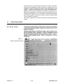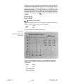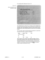
1
United States
Environmental Protection
Agency
Environmental Monitoring
Systems Laboratory
P.O. Box 93478
Las Vegas NV 89193-3478
Research and Development
ASSESS
User’s Guide
EPA/600/8-91/001
January 1991
NOTICE
Version 1.0 of this software is a prototype. Additional modifications are
planned for the future. The information in this document does not represent
the views or policy of the Environmental Protection Agency.
DISCLAIMER
ASSESS software and documentation are provided “as is” without guarantee or warranty of any kind, expressed or implied. The Environmental
Monitoring Systems Laboratory, U. S. Environmental Protection Agency
and Computer Sciences Corporation will not be liable for any damages,
losses, or claims consequent to use of this software or documentation.
ASSESS 1.0
ii
DECEMBER 1990
Contents
Contents . . . . . . . . . . . . . . . . . . . . . . . . . . . . . . . . . . . . . . . . . . . . . . . . . . . . . . . . . . . . . . . . . . . . . . . . . . . . . . . . . . . . . . . . . . . . . . . . . iii
List of Figures . . . . . . . . . . . . . . . . . . . . . . . . . . . . . . . . . . . . . . . . . . . . . . . . . . . . . . . . . . . . . . . . . . . . . . . . . . . . . . . . . . . . . v
1.
Introduction
2. System Operation
1.1 OVERVIEW . . . . . . . . . . . . . . . . . . . . . . . . . . . . . . . . . . . . . . . . . . . . . . . . . . . . . . . . . . . . . . . . . . . . . . . . . . . . . . . . . . 1-1
1.2 EQUIPMENT REQUIREMENTS . . . . . . . . . . . . . . . . . . . . . . . . . . . . . . . . . . . . . . . . . . . . . . . . . . 1-3
1.3 USER PROFILE . . . . . . . . . . . . . . . . . . . . . . . . . . . . . . . . . . . . . . . . . . . . . . . . . . . . . . . . . . . . . . . . . . . . . . . . . . . 1-3
1.4 INSTALLING THE SYSTEM . . . . . . . . . . . . . . . . . . . . . . . . . . . . . . . . . . . . . . . . . . . . . . . . . . . . . . . . 1-3
1.4.1 ASSESS Data Files . . . . . . . . . . . . . . . . . . . . . . . . . . . . . . . . . . . . . . . . . . . . . . . . . . . . . . . . . 1-3
1.4.2 Hard Disk Installation . . . . . . . . . . . . . . . . . . . . . . . . . . . . . . . . . . . . . . . . . . . . . . . . . . . . . 1-4
1.4.3 Using ASSESS on Floppy Diskette . . . . . . . . . . . . . . . . . . . . . . . . . . . . . . . 1-4
1.4.4 Using ASSESS from DOS . . . . . . . . . . . . . . . . . . . . . . . . . . . . . . . . . . . . . . . . . . . . . . 1-4
1.5 GRAPHICS . . . . . . . . . . . . . . . . . . . . . . . . . . . . . . . . . . . . . . . . . . . . . . . . . . . . . .1-4
1.5.1 On-Screen Graphics . . . . . . . . . . . . . . . . . . . . . . . . . . . . . . . . . . . . . . . . . . . . . . . . . . . . . . . 1-4
1.5.2 Metacoda-Based Graphics . . . . . . . . . . . . . . . . . . . . . . . ..1-4
1.6 ERROR AND RECOVERY PROCEDURES . . . . . . . . . . . . . . . . . . . . . . . . . . . . . . . . 1-5
2.1 DATA . . . . . . . . . . . . . . . . . . . . . . . . . . . . . . . . . . . . . . . . . . . . . . . . . . . . . . . . . . . . . . . . . . . . . . . . . . . . . . . . . . . . . . . . . . 2-1
2.1.1 ASSESS Data Files . . . . . . . . . . . . . . . . . . . . . . . . . . . . . . . . . . . . . . . . . . . . . . . . . . . . . . . . . 2-1
2.2 INTERACTIVE SCREENS . . . . . . . . . . . . . . . . . . . . . . . . . . . . . . . . . . . . . . . . . . . . . . . . . . . . . . . . . . . 2-2
2.2.1 Screen Format . . . . . . . . . . . . . . . . . . . . . . . . . . . . . . . . . . . . . . . . . . . . . . . . . . . . . . . . . . . . . . . . . 2-2
2.2.2 Types of Screen input Fields . . . . . . . . . . . . . . . . . . . . . . . . . . . . . . . . . . . . . . . . . 2-3
2.2.3 The Menu Tree . . . . . . . . . . . . . . . . . . . . . . . . . . . . . . . . . . . . . . . . . . . . . . . . . . . . . . . . . . . . . . . . 2-4
2.2.4 ASSESS Screens and Menus . . . . . . . . . . . . . . . . . . . . . . . . . . . . . . . . . . . . . . . . 2-4
3. Using ASSESS in an
Assessment Study:
Example
3.1 OVERVIEW . . . . . . . . . . . . . . . . . . . . . . . . . . . . . . . . . . . . . . . . . . . . . . . . . . . . . . . . . . . . . . . . . . . . . . . . . . . . . . . . . . 3-1
3.2 THE EXAMPLE SET . . . . . . . . . . . . . . . . . . . . . . . . . . . . . . . . . . . . . . . . . . . . . . . . . . . . . . . . . . . . . . . . . . . . 3-2
3.3 DATA INPUT THROUGH THE KEYBOARD: AN EXAMPLE . ..3-13
3.4 ALTERNATIVE DESIGN: AN EXAMPLE . . . . . . . . . . . . . . . . . . . . . . . . . . . . . . . . . . 3-15
Appendix A - DATA FILES . . . . . . . . . . . . . . . . . . . . . . . . . . . . . . . . . . . . . . . . . . . . . . . . . . . . . . . . . . . . . . . . . A-1
Appendix B - REFERENCES . . . . . . . . . . . . . . . . . . . . . . . . . . . . . . . . . . . . . . . . . . . . . . . . . . . . . . . . . . . . . . B-1
Appendix C - NOMENCLATURE . . . . . . . . . . . . . . . . . . . . . . . . . . . . . . . . . . . . . . . . . . . . . . . . . . . . . . . . C-1
ASSESS 1.0
iii
DECEMBER 1990
Page
Number
ASSESS 1.0
2-1
Example Interactive Screen . . . . . . . . . . . . . . . . . . . . . . . . . . . . . . . . . . . . . . . . . . . . . . . . . . . . . . . . . . . 2-2
2-2
The Menu Hierarchy . . . . . . . . . . . . . . . . . . . . . . . . . . . . . . . . . . . . . . . . . . . . . . . . . . . . . . . . . . . . . . . . . . . . . . . . 2-5
3-1
ASSESS Main Screen . . . . . . . . . . . . . . . . . . . . . . . . . . . . . . . . . . . . . . . . . . . . . . . . . . . . . . . . . . . . . . . . . . . . . 3-3
3-2
Sampling Considerations Screen . . . . . . . . . . . . . . . . . . . . . . . . . . . . . . . . . . . . . . . . . . . . . . . . . . 3-4
3-3
Historic Assessment Screen . . . . . . . . . . . . . . . . . . . . . . . . . . . . . .... . . . . . . . . . . . . . . . . . . . . . . . 3-5
3-4
3-5
Quality Assessment Data Screen . . . . . . . . . . . . . . . . . . . . . . . . . . . . . . . . . . . . . . . . . . . . . . . . . . 3-6
Scatter Plot of the QA Data . . . . . . . . . . . . . . . . . . . . . . . . . . . . . . . . . . . . . . . . . . . . . . . . . . . . . . . . . . . . 3-7
3-6
Transforms Screen . . . . . . . . . . . . . . . . . . . . . . . . . . . . . . . . . . . . . . . . . . . . . . . . . . . . . . . . . . . . . . . . . . . . . . . . . 3-8
3-7
The Scatter Plot of the Log Transformed Data . . . . . . . . . . . . . . . . . . . . . . . . . . ...3-8
3-8
The Results Screen . . . . . . . . . . . . . . . . . . . . . . . . . . . . . . . . . . . . . . . . . . . . . . . . . . . . . . . . . . . . . . . . . . . . . . . . . 3-10
3-9
The Intermediate Results Screen . . . . . . . . . . . . . . . . . . . . . . . . . . . . . . . . . . . . . . . . . . . . . . . . . . 3-11
3-10
The Error Bar Graph . . . . . . . . . . . . . . . . . . . . . . . . . . . . . . . . . . . . . . . . . . . . . . . . . . . . . . . . . . . . . . . . . . . . . . . 3-11
3-11
The Results Screen . . . . . . . . . . . . . . . . . . . . . . . . . . . . . . . . . . . . . . . . . . . . . . . . . . . . . . . . . . . . . . . . . . . . . . . . . 3-14
3-12
Alternative Design Results Screen . . . . . . . . . . . . . . . . . . . . . . . . . . . . . . . . . . . . . . . . . . . . . . . . 3-15
3-13
Alternative Design Error Bar Graph . . . . . . . . . . . . . . . . . . . . . . . . . . . . . . . . . . . . . . . . . . . . . . 3-16
3-14
Variance Estimates for the Alternative Design . . . . . . . . . . . . . . . . . . . . . . . . . . . . 3-17
v
DECEMBER 1990
1.1
OVERVIEW
ASSESS is an interactive program designed to assist the user in statistically
determining the quality of data from field samples. The program permits
quality assessment data and historical information (historical information is
for notational purposes only) such as data quality objectives, sampling
considerations, and historical assessments to be saved. Measurementerror variances are computed. Scatter plots of the variance (represented as
K times the standard deviation) versus the average concentration may be
produced for Routine Samples (RS) with either Field Duplicates (FD) or
Preparation Splits (PS). Transforms may be applied to the entire data set.
Error bar graphs of variance estimates from quality assessment (QA)
samples may be produced. Hardcopies of all plots may be obtained by
depressing the <P> key. The plots may also be stored in a file of device
independent plotting commands (metacode). An HPGL plotter instruction
file may be produced using the program HPPLOT with the metacode file as
input. The historical information, measurement-error variances, and data
set maybe written in a report format to either an output file or sent to a printer.
The printer must be either an Epson- or lBM-compatible dot matrix printer,
HP Laserjet, or HP Deskjet.
ASSESS may be used to provide a foundation for answering two basic
questions:
How many, and what type, of samples are required to assess the quality of
data in afield sampling effort? How can the information from the QA samples
be used to identify and control sources of error and uncertainties in the
measurement process?
Once the analytical results are received, bias and precision values will be
computed. Note that ASSESS will only compute the precision.
An alternative QA design that does not employ field evaluation samples
(FES) and external laboratory evaluation samples (ELES) is also discussed
and error variances are computed.
ASSESS uses two temporary files called scratch files to store and process
data read from an ASSESS data file. These scratch files are assigned the
names XXXXXXXX.XXX and ZZZZZZZZ.ZZZ.
The concentrations (units) of the samples may be specified for notational
purposes, but unit conversions cannot be made by ASSESS.
ASSESS 1.0
1-1
DECEMBER 1990
It is recommended that the EPA publication “A Rationale for the Assessment of Errors in the Sampling of Soils”(l), from which the program
ASSESS has been derived, be used in conjunction with this user manual.
Please forward any questions, comments, or bug reports to the following
address:
Jeff van Ee (Assess)
USEPA EMSL-LV, EAD
P.O. Box 93478
Las Vegas, NV 89193-3478
ASSESS 1.0
1-2
DECEMBER 1990
1.2
EQUIPMENT REQUIREMENTS
ASSESS was designed to run under DOS (Disk Operating System) on an
IBM PC, XT, AT, PS2, or compatible. Graphics capability is not required, but
is highly recommended as graphics output is produced. Graphics support
is provided for the Hercules graphics card, laptops with monochrome
displays having graphic capabilities, the Color Graphics Adapter (CGA),
and the Enhanced Graphics Adapter (EGA). Support for Video Graphics
Array (VGA) is not available, however, VGA does emulate EGA and
therefore graphics support is provided for VGA indirectly. At least 512
kilobytes (Kb) of random access memory (RAM) is required, but 640 Kb is
recommended. An arithmetic co-processorchip is recommended due to t he
computational intensive nature of the program, but is not required for use.
ASSESS may be run from floppy diskette or from a fixed disk. The system
storage requirement is approximately 420 kilobytes. For a hardcopy of
results, a graphics printer (IBM graphics compatible) is required. Support
is provided for plotters which accept HPGL plotting commands.
1.3
USER PROFILE
To use ASSESS, one should have some familiarity with personal computers
and DOS (Disk Operating System). One should also understand basic DOS
commands such as DIR (directory), CD (change directory), and how to
insert and use diskettes. For more information on these topics, consult a
DOS user’s manual. The manual titled “A Rationale for the Assessment of
Errors in the Sampling of Soils”(1) must be followed. For a list of references,
refer to Appendix B, References.
1.4
INSTALLING THE SYSTEM
1.4.7 ASSESS Data Files
ASSESS in its executable form is entirely in the public domain. In the future,
it may be downloaded from the U.S. EPA Bulletin Board System.
ASSESS. exe is the only file required to run ASSESS. If a metacode file is
to be converted to a file with an HPGL format, then Hpplot.exe and
Hershy.bar are required. Hershy.bar is a character font file and is required
to execute Hpplot.exe.
The executable file, example data set, and optional files are as follows:
ASSESS
422778 bytes (required)
Optional:
Alt1
Alt2
Saved1
Saved2
Scatter
Results
Smdata
Example
Hpplot
Herahy
.fil
2576
1471
.fil
.fil
1636
.fil
4744
.fil
3771
1440
.met
.met
2880
.fil
4744
.fil.
1714
4744
.fil
.exe
98417
.bar 176000
bytes
bytes
bytes
bytes
bytes
bytes
bytes
bytes
bytes
bytes
bytes
bytes
(example data set)
(example data set)
(example data set)
(used for comparison)
(used for comparison)
(wad for comparison)
(used for comparison)
(used for comparison)
(example data set)
(example data set)
(conversion program)
(required with Hpplot.exe)
The files denoted as “Used for Comparison” will be created by ASSESS as
you run through the program. Therefore, these files may reside somewhere
ASSESS 1.0
1-3
DECEMBER 1990
outside the directory where ASSESS resides and thus will not be overwritten.
The source code is written in FORTRAN 77 for the Microsoft (Microsoft
Corporataion, Redmond, WA) FORTRAN compiler (version 4.01 ). With the
exception of slightly modified proprietary Graflib Version 1.0 (Sutrasoft,
Sugarland, TX) subroutines used for generating screen graphics, the
source code is also in the public domain.
1.4.2 Hard Disk Installation
To install the system on a fixed disk, a subdirectory should first be
created (for example, ASSESS). Copy ASSESS. exe and any other
optional files into the subdirectory. For more information on creating
subdirectories and copying files from a diskette into a subdirectory, refer
to your DOS user’s manual.
1.4.3 Using ASSESS on
Floppy Diskette
ASSESS. exe is too large to fit on a 360 kilobyte diskette. This means
that if only a 360 kilobyte disk drive (and no fixed disk) is available, then
ASSESS cannot be used. Either a 3.5 disk drive or a 1.2 megabyte (or
larger) 5.25” disk drive is needed to run both ASSESS and the optional
program Hpplot.exe (with Hershy.bar)
1.4.4 Using ASSESS from
DOS
To run ASSESS or Hpplot from DOS, type ASSESS or Hpplot at the
DOS prompt. For example, to start program ASSESS type:
ASSESS uses most of the available memory. If an error message occurs
after typing ASSESS, try to free other existing memory-resident programs,
and type ASSESS to restart the program.
1.5
GRAPHICS
1.5.1 On-Screen Graphics
1.5.2
Metacode-Based
Graphics
ASSESS 1.0
ASSESS plots graphics directly on the screen. This approach is used to
provide a quick look at data or program results. Such graphics displays may
be printed on a dot-matrix printer. When a graphics screen is displayed, the
program will wait for a key to be pressed. Pressing <Q> will cause an
interactive screen and menu to be displayed. Pressing <P> will produce a
hard copy of the screen on a graphics printer. It is important to make sure
that a graphics printer is connected to your computer if you choose this
option, or the program will “lock-up”. Also make sure t hat the printer is turned
on and “on-line”. If the program “locks up”, the computer will probably have
to be re-started.
The graphics displays may also be written to a “metacode” file when the
“Save Plot” menu option is selected. A metacode file is a file of deviceindependent plotting instructions. This file can be converted to a HPGL
(Hewlett Packard Graphics Language) formatted file using the program
Hpplot (refer to section 1.4.1 ASSESS Data Files concerning Hpplot.exe).
The advantage of using a metacode file is that higher-quality graphic output
can be obtained on a pen plotter or other graphics device. The HPGL format
is directly supported by WordPerfect.
1-4
DECEMBER 1990
1.6
Example: To import a 1.)
metacode file generated by
ASSESS into
WordPerfect 5.0*, perform the
following steps
Generate a metacode file called ‘Metacode.met’ using ASSESS.
Either of the two graphs generated by ASSESS may be saved to a
metacode file. Note that the name “Metacode.met” is a generic name
and it may be referred to by any other name. The ‘met” extension is
used as a means of distinguishing these files and the regular ASCII text
files.
2.)
Run the program HPPLOT. Enter ‘Metacode.met’ as the input file and
‘Metacode.pit’ as the output file. HPPLOT will convert ‘Metacode.met’
to an HPGL formatted filecalled ‘Metacode.plt’, which is supported by
WordPerfect*.
3.)
If you have a VGA adapter, the HPGL formatted file may require one
more conversion using the WordPerfect conversion program
Graphcnv,exe. To convert, call GRAPHCNV, and then enter
“Metacode.pit” as the input file and “Metacode.wpg” as the output file.
GRAPHCNV will generate “Metacode.wpg” which can be successfully
imported into WordPerfect on PC’s using a VGA adapter.
ERROR AND RECOVERY PROCEDURES
Normal Error Processing
ASSESS performs error checking on such items as file existence, file Input/
Output and bounds checking on numeric parameters. When errors of these
types are encountered in programs, error messages are displayed on the
message line at the bottom of the screen. These messages are displayed
in a black-on-white format (reverse video) and are accompanied with a buzz
sound. To return to the interactive screen after such a message is displayed,
press any key.
Problems
Although ASSESS has been tested and debugged it is still possible that
there are situations which will cause ASSESS to “crash” or “fail” (terminate
prematurely), or to “lock-up” (pause indefinitely with no response). If
ASSESS “locks-up”, the computer must be re-started. The problem may be
due to a bug, or due to a printer or disk-drive problem (see below).
ASSESS may crash when a binary operation in the Transform menu is
chosen which would produce a very large or very small number. An example
would be the operation 1.0/X, or 10 to the power of X, when X is a very small
or very large (1.E-l 000, 1.E1 000). This type of program error cannot be
trapped or handled by ASSESS. In such cases the result cannot be
produced due to hardware limitations in the precision of the numeric
coprocessor (or floating-point emulation software). Since there is no remedy
for this situation, the only solution is to avoid such operations.
There are several error conditions which the program was specifically not
designed to check for. These involve checking to see if disk or printer
peripherals are connected and ready for data transfer. The user should
ensure that printers are attached and on-line, or that disk drives have the
correct density media and are ready for read/write operations, when Read,
Save, or Write options are selected. The following actions are guaranteed
to create a “lock-up” situation.
*WordPerfect is a registered trademark of WordPerfect Corporation.
ASSESS 1.0
1-5
DECEMBER 1990
Trying to print a text or graphics screen when the printer is not
connected or on-line. If a printer is connected, make sure it is turned
“on” and is ready to accept output from the computer (on-line). If a
printer is not connected to your system, it may be necessary to “reboot” the computer.
Accessing a file on a floppy diskette drive when the disk drive door is
open, or no diskette is present. In some cases, DOS may respond
with a message: Device not ready (Abort, Retry, Ignore). Insert a
diskette and press <R> (for Retry). If this does not work, you must restart the computer.
ASSESS 1.0
1-6
DECEMBER 1990
2.1
DATA
2.1.1 ASSESS Data Files
ASSESS employs a particular format for its data files. An ASSESS data file
is an ASCII text file and is different from the Metacode files used by the
HPPLOT program. The ASSESS data files may be created with any text
editor. For instance, WordPerfect* files may be converted to ASCII text files
before being supplied to the program. Make sure your data files are
compatible with the input format, or the program will not be able to read them,
ASSESS will also operate without an input data file, in which case the screen
layout for data input will be self explanatory. Three example data files
included with the distribution diskette will be used as examples in this
manual. Copy these files into the subdirectory where the Program ASSESS
resides. They are called “standard. fil”, “(altl .fil”, and “smdata.fil”. Below is
an explanation of the “standard. fil’’data file. The format of the other two files
is the same and will be discussed later. It is helpful to obtain a print-out of
these files using the DOS print command before proceeding to the next
section.
Line 1 to 42
These lines of data represent the historical information. The data file
includes information about the site, methods, desired accuracy, precision,
etc. Note that these input lines are inconsequential to the data processing
phase of ASSESS and are merely supplied to keep track of sampling
considerations and historical assessments.
Line 43 to End of File - The Data Entries
This is where the data are stored. Each row represents a batch sample
consisting of a pair of QA samples. For the regular design, these QA
samples are stored under the following columns: Routine Sample (RS),
Field Duplicate (F D), Preparation Split (PS), Field Evaluation Sample Pairs
(FES1 and FES2), and External Laboratoy Evaluation Sample pairs (ELES1
and ELES2).
For the “Alternative QA design, only FES1 and ELES1 values used for
detection of bias are included; and two new columns are provided for Batch
Field Duplicates (BFD) and their locations.
*WordPerfect is a registered trademark of WordPerfect Corporation.
ASSESS 1.0
2-1
DECEMBER 1990
The data may be in “free format” which means that in a given line in the file,
values must be separated by at least one space or a single comma. For
readability, columns of numbers should line up; although this style is not
required. Variable values must be numeric with no embedded blanks.
Whenever a value could not be obtained for a variable, a special value of 9999.0 will be assigned to it. This value, referred to as missing, will not be
included in the calculations. The file “standard.fil’’ contains the historical data
and 23 batch samples. Examine the contents of this file using the DOS
“Type” command or your editor.
Note: Refer to Appendix A for further discussions of the different data file
formats.
2.2
INTERACTIVE SCREENS
2.2.1 Screen Format
Figure 2-1
Example Interactive Screen
ASSESS 1.0
2-2
DECEMBER 1990
The Screen Frame
This is the rectangular box which encloses each screen. Program
inputs and results are displayed in this area. Typically, the screen frame
is divided into smaller, single-line rectangles. Each of these smaller
rectangles contains a functionally related group of one or more input
parameters or program results.
The Message Line
This is the rectangle at the bottom of the screen frame. This area is used
to display program error messages, yes/no prompts, prompts for
additional information, or instructions for using a program option.
The Menu Line
This is the line of text just below the screen frame. It contains a set of
menu option names and a highlighted box (cursor bar). The cursor bar
can be moved along the menu line by using the <left> and <right> arrow
keys. As the cursor bar is moved over a menu option name, a short
description of the menu option is displayed on the line just below the
menu line. This line is called the menu description line. You may
explore the possible choices in a program by moving the cursor bar and
reading the descriptive messages which accompany each menu option. To select a menu option, move the cursor bar over the desired
menu option name, and press <enter>. An alternative (and faster) way
to select a menu option is to press the key which corresponds to the first
letter in the menu option name. The result is the same as using the
cursor control keys and pressing <enter>. For example, you would
choose the “Revise” option by pressing <R> from the main menu.
Parameter Groups
Typically, a functionally related group of program input parameters
(fields) are enclosed together on the screen by a single-line rectangle.
These groups of parameters are accessed through the menu. When a
menu option is selected, a cursor bar appears at the screen field, and
a message describing what action to take appears on the message line.
When such a group contains several fields, the cursor control keys are
used to move to subsequent fields. Exiting from the last field in the
group will return the cursor bar to the menu line.
2.2.2.
Types of Screen input
Fields
Several types of input files are provided to allow flexibility in program
parameter specification. Below is a list of these types and an example of
each field type in the first screen of ASSESS (Figure 2-1).
Alphanumeric Fields — These fields may contain character strings of
alphabetic or numeric characters. Any alphanumeric characters may
be entered. The ‘Data” menu option in the screen of Figure 2-1 requires
an alphanumeric value to be entered. To specify a data file name, select
the data option on the menu; and type the name of the input data file.
ASSESS 1.0
2-3
DECEMBER 1990
Numeric Fields — Only numeric data may be entered into numeric fields.
Some numeric fields will only accept integer (non-decimal) numbers.
The program will respond to any erroneous keystrokes (such as
alphabetic keys) with a low-pitched error tone. An example of numeric
fields in the screen of Figure 2-1 are the desired accuracy and desired
precision fields. Only integers may be entered for these two fields.
Toggle Fields — A toggle field is a special type of field which contains a list
of 2 or more preset choices. Only one of these choices is displayed in
the field. The <space> key is used to change the displayed choice, and
the <enter> key is used to make the selection. Two examples of toggle
fields in the screen of Figure 2-1 are the “Data’’ field and the “Alternative”
field. Once the data option is selected, the toggle field will contain a
“Yes” and “No” in response to the prompt “Do you want to specify a data
file <use space bar>:” The toggle field will be highlighted; and each time
the <space> key is pressed, “Yes” or “No” will appear. Press the
<enter> key to make a selection. If “Yes” is selected, the toggle fields
“Input (with labels)” and “Standard (with no labels)” may then be
selected. Alternative option allows for two toggle fields, “Yes” and “No”,
in response to the prompts regarding the sample locations.
Yes/No prompts, prompts for additional information — These prompts
are for information which will not be displayed permanently on the
screen. They will appear temporarily on the message line. A Yes/No
prompt will typically have the form: “Question...<Y/N>?”. To respond
Yes, press the <Y> key; to respond in the negative, press any other key.
A typical Yes/No prompt is the “Do you really want to quit <Y/N>?”
prompt which is displayed after the “Quit” (terminate program) option is
selected. Another example is when you attempt to write over an existing
file.
2.2.3 The Menu Tree
ASSESS typically requires input from data files and through interactive
screens. These program inputs are arranged in a hierarchy of functionally
related groups. Each group or individual program parameter value is
accessed through a menu of choices. Some choices will lead to other
menus, while some will lead to prompts for groups of one or more inputs.
Such an arrangement can be represented in a menu hierarchy as illustrated
in Figure 2-2.
The “menu tree” representation of program options provides a “road map”
for ASSESS which summarizes the functional capabilities of a program. You
may explore the hierarchy of options by traversing the menu tree and
reading the descriptive messages which appear at the bottom of each
screen.
2.2.4
ASSESS Screens and
Menus
ASSESS 1.0
ASSESS initially displays an introduction screen. Upon pressing any key,
the first interactive screen is displayed. The information entered or displayed
on the succeeding three screens, namely the “Data Quality Objectives”
screen, the “Sampling Considerations” screen and the “Historical Assessment” screen, are used presently for information purposes. No calculations
are performed using the information from these three screens. The information is written to a user-specified file, along with the results of other
calculations.
2-4
DECEMBER 1990
Figure 2-2
t
ASSESS 1.0
I
1
,
I
2-5
I
I
DECEMBER 1990
3.1
OVERVIEW
This section will demonstrate how to use the ASSESS software to conduct
an assessment study. We start with an example data set obtained from an
actual Superfund site which was contaminated by lead deposition from a
smelter; however, the arrangement of the data into batches and data from
field evaluation samples are fictional and are included for illustrative purposes.
Through this example data set, we will explore the ASSESS utilities and
analyze its results. Two other data sets for the alternative QA design will also
be shown. The data set “standard.fil” has been included with the software,
so that you may repeat the exercise as a tutorial or to test the software. For
a detailed explanation oft he data, refer to the “Rationale document”(l).
The pilot study was conducted over a representative area to determine
spatial variability and extent of the lead contamination in order to develop an
efficient sampling network for obtaining representative measurements of
contamination over a large area. The quality assessment program was
implemented to assess variability from the collection, handling, and analysis
of the samples.
ASSESS 1.0
3-1
DECEMBER 1990
3.2
THE EXAMPLE DATA SET
The “standard.fil” data set is an ASCll file in the ASSESS format. It contains
data grouped into 23 batches. The file structure is described in Section 2.
The first few lines of data without the historical information are as follows:
1
−9999.000 −9999.000 −9999.000 448.000 505.000 −9999.000 −9999.000
2
−9999.000 −9999.000 −9999.000 475.000 488.000 −9999.000 −9999.000
3
−9999.000 −9999.000 −9999.000 423.000 424.000 −9999.000 −9999.000
389.000 −9999.000
4
430.000−9999.000−9999.000 −9999.000 −9999.000
Each row represents a batch. The first through the third rows indicate that
only Field Evaluation Sample pairs (FES1 and FES2) exist, and all other
samples are unknown (i.e., missing). The fourth batch indicates that only a
routine sample (RS) and a preparation split sample (PS) exist.
Notice that the ASSESS data files for the regular design consist of the
following columns in the given order: RS, FD, PS, FES1, FES2, ELES1,
ELES2.
Assuming that you have already copied the software and data into a
directory called ASSESS on your hard disk and have used the command
“CD\ASSESS” to access the directory, you can run ASSESS by typing the
command:
ASSESS <enter>.
When the program begins execution, it first displays a screen with
introductory information. When you press a key to proceed, you will see
the program main screen and menu as displayed in Figure 2-1.
The bottom line on the screen provides the list of available options. The first
three options move you to an area on the screen (or to a new screen) where
you can input or select program parameters.
We begin by running through the program using the menu options.
Throughout this tutorial you will seethe phrase “select an option” used often.
You “select” an option by positioning the cursor baron the option or field, and
pressing the <enter> key.
In the data analysis section of this document the following points are noted:
1. The line “Insufficient samples exist for this variance” for any error
variance estimates means that enough samples do not exist to assess
the variance.
2. if the value of any variance estimate is less than zero, a value of zero
will be assigned to that variance.
Data
The “Data” option is used to decide whether a data file is present or data is
to be entered on the screen. Select the data option and answer Yes to the
prompt “Do you want to specify a data file? (use <space> bar):”?. This is done
by pressing the <enter> key on the toggle field “Yes”. You are then asked
about the format of the input file. Hit the space bar to toggle through the
options, and select the “standard (with no Iabels)” field in response to the
“What is the input file format? (use <space> bar):” prompt. As before, select
ASSESS 1.0
3-2
DECEMBER 1990
a particular field by pressing the <enter> key. You are then prompted for a
data file name. Notice the cursor jumps to the “Datafile:” field on the screen.
Type the name of the input data file, which in this case is “Standard.fil”, and
press the <enter> key. A short tuned noise will be generated, and the
message “ERROR - data file not found (press any key)” will be displayed if
an incorrect or a non-existent file is entered. In such a case, select the Data
option and proceed with correct entries. The following screen will be
displayed (Figure 3-1 ).
Figure 3-1
ASSESS Main Screen
Alternative
This option allows the user to select the alternative QA design without the
FES and ELES values. Since the first example does not employ the
alternative design, DO NOT select this option. Use your cursor keys to move
to the “Revise” option.
Revise
This option is used to revise the screen parameters. Note that the
parameters on the second part of the screen displaying the site, method, etc.
are only for historical notations and have no bearing on the result of the
analysis. Note also that the displayed information is the result of the input
given in the file “standard.fil”. You may proceed to the next option by not
selecting the “Revise” option, thus accepting the listed parameters. However, for illustration purposes, select the “Revise” option, move the cursor
key to the “Analyte:’’ field, and type in “lead’’ over “Pb” and press the <enter>
key. Pressing the <enter> key till the end of the screen parameters or the
<left arrow> key at anytime, will take you back to the “Revise*’ option on the
menu fields.
Sampling Considerations
This option displays the “Sampling Considerations” menu. It is designed
only for historical notations, and is merely a summary of the contents of parts
ASSESS 1.0
3-3
DECEMBER 1990
of the data file. DO NOT this option yet. We will discuss this after
examining the remaining options on the screen.
Evaluate Data
This option displays the “Evaluate Data” menu. Through this menu,
ASSESS does all of its computing work. It computes and displays measurement error variances. It also performs data transformations, produces
reports and plots data. This option may be selected immediately after the
specification of data input type and will bypass the sampling consideration
and historical assessment screens. Experienced users will select this opt ion
first if quick data evaluation is required, thus bypassing the historical
screens.
Quit
This option is used to exit the program. Using the analogy of the menu tree,
the “Quit’’ option also allows you to “move up’’ one level in the tree. The “Quit”
option will also appear in other successive screens. When this option is used
from the main menu of the program, a Yes/No prompt is issued: “Do you
really want to quit <Y/N>?”. The <Q> key is typically used to select this
option. The Yes/No prompt is a means of ensuring that a series of <Q>
keystrokes will not cause inadvertent termination of the program.
You may now select the “Sampling Considerations” option from the menu
bar. The following screen will be displayed:
Figure 3-2
Sampling Considerations
We will now discuss the options accessed through this screen.
Revise
This option is exactly similar to the discussion of the “Revise” option above.
Let us change the analysis cost to $500.00. Select the “Revise” option, use
ASSESS 1.0
3-4
DECEMBER 1990
the <down arrow> key to move to the “Analysis” field, and type 500.00.
Notice that if you hit an <ente~ key after entering the number 500.00, you
will be placed into the next part of the screen regarding the batch data. To
get back to the “Revise” option, move your cursor bar to the extreme left or
right sides of the screen frame using the arrow keys.
Historical Assessment
This option displays the “Historical Assessment” menu. This menu shows
a screen with the bias and measurement data of the input data file. DO NOT
select this option yet. We will discuss it after examining the remaining
options on the screen.
Evaluate Data
This option is exactly similar to the option discussed for the main screen.
Quit
This option will return the user to the main menu of the main screen.
We may now select the “Historical Assessment” option. After pressing the
<enter> key on the “Historical Assessment” option, the following screen will
be displayed.
Figure 3-3
Historical Assessment Screen
We will now discuss the options accessed through this screen.
Revise
Through this option, you may alter any of the screen fields as discussed in
the previous explanation of Revise. Select the “Revise” option, and change
the “Total Measurement Variance:” field to 0.09.
ASSESS 1.0
3-5
DECEMBER 1990
Evaluate Data
This option is essentially the same as previously discussed.
Quit
This option will return you to the previous menu which is the “Sampling
Considerations” screen.
We will now select the “Evaluate Data” menu option to display the “Quality
Assessment Data” screen.
Figure 3-4
Quality Assessment Data
The screen above shows the contents of your input data file. It only shows
data for 10 batches within the RS, FD, and PS columns. The “Scroll” option
described below will let you explore the additional batches and the remaining
columns not seen on the screen.
We will now discuss the options accessed through this screen.
Units
This option will allow you to enter the concentration unit. Select this option
and type “mg/kg”. When you hit the <enter> key after typing in the
concentration unit, you will be back on the units option.
Scroll
This option will allow you to scroll through the input screen. The data file
“standard.fil” contains 23 batches, but only 10 are shown on the screen.
Select the “Scroll” option. In the message frame, you will notice the message
“Use <arrow> key to scroll or <Q> to Quit.” As you push the <right arrow>
key, you will notice that additional columns of input will appear on the screen.
Note that missing values are represented by blanks on the screen, thus
improving readability. The <down arrow> key will let you scroll and observe
additional batches, if any. After scrolling through the screen, press the letter
<Q> to get back to the “Scroll” option.
ASSESS 1.0
3-6
DECEMBER 1990
Revise
This option is the same as previously discussed. You may alter any of the
input values by a sequence of arrow keys (to get to the correct position) and
typing over the old values. Note that the “Save Data’’ option must be selected
to save any new changes before proceeding to transformations of the data,
or execution of the program. For the time being, do not alter any of the data.
Proceed to the following option.
Transform
The Transform option is used as a tool to determine if the data needs to be
transformed and to carry out various data transformations.
The “Transform” option plots a scattergram of the data. When the ‘Transform”
option is selected, you will have a choice as to the type of data to be plotted.
Select this option, and you will be prompted by “Specify plot of which
concentration to use? (use <space> bar):. Toggle through the possible
fields which are “RS&FD” and “RS&PS”. Remember to use the space bar
to toggle throughout the possible options. Select the “RS&FD” field and
press the <enter> key. Note the message on the message line, and press
any key to view the scattergram. The following is the plot of the original data
(untransformed).
Figure 3-5
Scatter plot of the QA data
Figure 3-5 illustrates the need for a transform of the original data. The plot
shows that the standard deviation of the data (multiplied by Z) from routine
samples and field duplicates increases with the average concentration of
these samples. A Iogarithmic transform of the data will stabilize the variance
of the data over measured concentration range. After this transformation
has occurred, the variances may be computed for the purpose of assessing
variability throughout the measurement process.
Press the letter <Q> to quit the graph, and observe the following "Transforms” screen.
ASSESS 1.0
3-7
DECEMBER 1990
Figure 3-6
Transforms Screen
Unary Operation
This option allows the user to toggle through five unary operations, as well
as a “Retain” option, which allows the original data to be retained thereby
eliminating any confusion as to the type of data being transformed. These
six options are also listed on the screen. Select the “Unary operation”, and
use the space bar to toggle through the possible selections. Select the “Ln”
operator to take the log base e of the original data. After selecting this option
you will remain in this screen. In order to view the newly created plot, select
the “Quit” option. Notice the message at the bottom of the screen when the
cursor bar is moved to the “Quit” option. This option will return you to the
“Quality Assessment Data” screen. Notice the data displayed on the screen.
The values are log base e of the original data. Select the “Transform” option
and the “RS&FD” toggle field. Press <enter> to view the following graph:
Figure 3-7
The Scatter P/et of the Log
Transformed Data
ASSESS 1.0
3-8
DECEMBER 1990
The data now fall along a straight horizontal line. The variance of the data
is now said to be “stabilized.
Press the letter <Q>, and select the “Quit” option to return to the “Quality
Assessment Data’’ screen. Notice that the screen shows the log-transformed
data of the input data.
In order to explore the remaining options of the ‘Transforms” menu, select
the “Transform” option. Select the “RS & PS’ ’toggle field and view the graph.
Press the letter <Q> to quit the graph and enter the ‘Transform” screen. The
“Unary Operation” option was discussed above. It may be used to retain the
original data, so that additional transforms may be applied to the
untransformed data.
Binary Operation
This option allows data transformation using the given binary operators on
the screen. This option has the same features as the “Unary Operation”
option, and allows you to perform multiplication, division, addition, subtraction, exponentiation, and retain the original data.
Save Plot
This option saves the generated plot through the “Transform” option. The
plot that will be saved is the plot just observed prior to reaching this screen
layout. Conceptually, it saves the plot that is no longer visible by the user,
though it still exists. in order to save the plot just viewed, select this option
and enter “Scatter.met” for the “Meta File:” prompt.
Quit
This option will return to the “Quality Assessment Data” screen. Select this
option to return to the “Quality Assessment Data” screen.
Execute
This option will display the results obtained by applying the equations in table
5 of the “Rationale Document”(l ). The primary purpose here is to estimate
measurement-error variance components. The measured lead concentrations in soil (in mg/kg) are given for 10 Preparation Spilt (PS) pairs and for
10 Field Duplicate (FD) pairs. The amount of data used has been kept small
for readability and to illustrate the use of the computer program to calculate
variances. Select the “Execute” option. The following screen will be
displayed:
ASSESS 1.0
3-9
DECEMBER 1990
Figure 3-8
The Results Screen
Figure 3-8 shows a summary of the results. Note that when enough
samples do not exist to assess any of the variances, “Insufficient samples
exist for this variance” will be displayed. For example, sample-collection
variance can not be calculated, because the error estimate calculated from
external laboratory evaluation samples (ELES) does not exist. Refer to
Table 5 of the “Rationale Document” (1) for the formulas. Also note that the
analytical variance could not be oomputed, since the estimate from external
laboratory evaluation samples (ELES pairs) can not be obtained. This
screen also displays a summary of the number of QA samples present.
Note that the number of ELES values is equal to zero.
The options on this screen will now be discussed.
Change Data
This option will return the user to the “Evaluate Data” menu to make
additional changes. The user will examine the result on the screen and
decide if changes are necessary, This option will not do anything
computationally, but is only a means for accessing the data screen. You
may select this option, if there is a need for additional changes. This option
will take you back to the “Quality Assessment Data” screen, After making
changes, the “Execute” option will bring you back to the “Results” screen.
This option will be selected after explaining the following options.
Var. Estimates
This option will display a screen showing the values of various variance
estimates. Select the “Var. Estimates” option. The following screen will be
displayed.
ASSESS 1.0
3-10
DECEMBER 1990
Figure 3-9
The Intermediate Results
Screen
The table shows the variance estimates given in Table 5 of the “Rationale
Document”(l). Press any key to return to the “Results” screen.
Plot
This option is used to display a plot of the error bar graph. (Note the
message on the message line.) Select the “Plot” option, and press any
key to view the following plot.
Figure 3-10
The Error Bar Graph
ASSESS 1.0
3-11
DECEMBER 1990
The plot illustrates the range in which the estimates of the various variance
components may be expected to occur within a 95% confidence interval. It
is clear from the length of the line for “sbfes” (Field Evaluation Samples
estimate) that greater use of field evaluation samples would have improved
the assessment of between-batch variability, as well as total measurement
error variance. Table 3 of the ‘ tRationale Document”(1) is used to determine
the 95% confidence intervals for variances based on the degrees of
freedom. Press the letter <Q> to return to the “Results” screen.
Save Plot
This option saves the error bar chart of the plot just viewed. Select this
option, and type in “barchart.met” in response to the “Mets File:” prompt.
After the metacode file has been written, press any key to return to the menu
bar. A Metacode file is a device-independent file used by the program
HPPLOT to produce a hardcopy of the plot on an HP plotter. Notice that you
may also press the letter <P> to produce a hardcopy of the plot (Make sure
that the printer is on-line). For more information on how to port this file into
WordPerfect, refer to section 1.5.2, and consult your WordPerfect manuals.
Report
This option generates a report of the data and its results in three formats.
The output may go to a file with input format, a file with report format, and
to the printer, Select this option and select the “file (report format)” toggle
field, Type in “results.fil” after the “Report File:” prompt.
Quit
This option will return the user to the main menu.
In order to return to the “Evaluate Data” menu, select the “Change Data”
option. You are now located at the “Quality Assessment Data” screen.
Save Data
This option allows the user to save the contents of the screen in a data file
with the input format. Select this opt ion, and type in “Saved1.fil” in response
to the “File:” prompt.
Quit
This option will return the user to the main menu. This is a good time to take
a break. Select the “Quit” option of the “Quality Assessment Data” screen.
The resulting screen is the main screen of ASSESS. Select the “Quit” option
to end this session of ASSESS. We will return to ASSESS to demonstrate
input from keyboard.
Now the basic concept of ASSESS has been studied, two shorter examples
dealing with input data from the keyboard and using alternative QA design
will be offered.
ASSESS 1.0
3-12 .
DECEMBER 1990
3.3
DATA INPUT THROUGH THE KEYBOARD: AN EXAMPLE
As discussed earlier, the second and third screens in ASSESS are used in
reviewing or revising the historical data. These two screens may be skipped
without any effects on the computational aspect of ASSESS. In this
example, we will allow the user to access the “Evaluate Data” menu, input
pair data, carry out computations and sketch plots, and finally save input
data at anytime during the calculation phase. Obtain a hardcopy of the file
“smdata.fil”. The data in this file will be used as input to the program. At the
DOS prompt in the appropriate subdirectory, type the command:
After observing the introductory screen, the screen of Figure 3-1 will be
displayed. In the previous section, the sequence of actions needed to
display various results were explained in a long-hand notation, where every
keystroke was thoroughly explained.
To simplify our explanations, an abbreviated notation for the sequence of
events will be used. A general formula exists for each option: Initiate the
option, then take one or more actions, each of which may result in a screen
field taking a particular value.
In order to get to the “Evaluate Data” menu, without a data file, use the
following set of actions:
Action Field
Value
Option
Enter
Data
Data File
No
Evaluate Data Enter
Number of Rows 13
Revise
Enter
Enter the values from the file “smdata.fil” using the <arrow keys> to move
the cursor bar. Notice that the first 42 lines are historical information and will
be ignored. You may pass over afield, thus assigning a missing value to that
particular field (“-9999.0” in the data file represents a missing value).
Notice that by pressing the <enter> key, you will be positioned at the
“Revise” option on the menu bar. Select it again to return to the input screen.
Once all of the data is entered, take the following actions.
Option
Action Field
Enter
Data file
Enter
Value
Saved2.fil
Save Data
Execute
The screen of Figure 3-11 will be displayed. Notice that through the “Save
Data” option, you may save your data at anytime. The format of this file is
“Input (with labels)”. This point is important if you would want to use this file
again to add or delete information. Therefore, on the first screen, you would
select the “Input (with labels)” toggle field of the Data Option, if there is a
need to use this file as input to ASSESS. This example is used to verify your
results. Analysis of data is similar to the analysis discussed in the previous
section.
Quit
Quit
ASSESS 1.0
Enter
Enter
3-13
Quit Prompt
Y
DECEMBER 1990
Figure 3-11
The Results Screen
ASSESS 1.0
3-14
DECEMBER 1990
3.4
ALTERNATIVE DESIGN: AN EXAMPLE
The alternative QA design was developed to assess measurement error
variances in absence of FES and ELES pairs. Formulas in Table 6 in the
“Rationale Document”(l) are used to calculate the results. The required
data for the alternative design are RS, FD, PS, BFD (Batch Field Duplicates),
the location of BFD values, and FES1, and ELES1 values. The FES1 and
ELES1 values are not used in the computations and are only used to
represent bias. Note: ASSESS presently does not calculate bias in the data.
In the following example the data file “Alt1.fil” is used to illustrate the case
where batch field duplicates are all obtained from one sampling location.
The format of the file “Alt1.fil” is the same as for the data file “standard.fil”.
Take the following sequence of actions to display the variance estimates,
produce error bar graphs and scattergrams.
Option
Data
Action Field
Value
Enter
Yes, Standard (with no
Iabels), Alt1.fil
Data File
Alternative
Enter
Sample Location
Yes, No
If you answer either “Yes” to both questions or “No” to both, you will be
notified by an error message asking you to start over. Cursor bar returns
to “Data” option.
Evaluate Data Enter
Execute
Enter
The following screen will be displayed.
Figure 3-12
Alternative Design Results
Screen
ASSESS 1.0
3-15
DECEMBER 1990
Note that the variance component associated with handling cannot be
separated from that associated with sample collection, and that the variance
component associated with subsampling cannot be separated from that
associated with analysis. This loss of information is a consequence of not
using FES and ELES values in the study. The sampling and handling
variance is equal to zero. This variance is the result of subtracting the error
estimate for the preparation splits s~~ from the error estimate for the field
duplicates.
For this example
~ +~ = 2.793-27.188 = -24.395
ASSESS will report a value of zero, when the measured variance is a
negative number. Follow the sequence of keystrokes:
Option
Action
Plot
Enter
The resulting graph is displayed in Figure 3-13.
Figure 3-13
Alternative Design Error
Bar Graph
Notice the large confidence interval for the preparation split samples.
Perhaps more preparation split samples could be taken to reduce this
large interval.
Option
Action
<Q>
Enter
Var. Estimates Enter
Press any key Enter
ASSESS 1.0
3-16
DECEMBER 1990
The resulting table is displayed in Figure 3-14.
Figure 3-14
Variance estimates for the
Alternative Design
The displayed data in this figure is a summary of the computed error
estimates for the alternative design. Note that the estimate for the batch field
duplicates is the one computed for condition (a). This condition is appropriate when the batch field duplicates are all taken from one sampling
location.
You may end this session by the following given keystrokes or proceed with
the data transformation as previously discussed.
Option
Action Field
Value
Press any key Enter
<Q>
Enter
<Q>
Enter
Prompt
Yes
The file “Alt2.fil” is also included in the distribution diskette. This file
contains data necessary to carry out the alternative design where Field
Duplicate Samples are taken from different locations. Table (6) of the
“Rationale Document”(l) is used for the calculations. Note that for this
design the error estimate for batch field duplicate (s~~~ is calculated
using the equation denotated for part (b).
ASSESS 1.0
3-17
DECEMBER 1990
The data files are simple ASCII text files which may be created with any text
editor, and can be printed using the DOS print command. ASSESS can
produce two types of output files; both of which contain the historical
information (for notational purposes only) displayed on the screens, the
summary of results, and the quality assessment data. One of these output
files can be read in as a data file by ASSESS (see “Example.fil”, next page),
whereas the other output file uses a report- like format (see Report of Results
which follows) and is not readable by ASSESS. A third file (see “Standard.fil”
which follows), produced only by the user, is readable by ASSESS but lacks
the descriptive labels included in the other two output files. The third file type
is provided so that the user may edit an input file without having to enter all
the data via ASSESS; (this method is faster in cases where the number of
quality assessment data is large).
Two example data files are provided. As noted above “Example.fil” is an
example of a file generated by ASSESS that can be used as an input file.
When selecting the Data option in the Data Quality Objectives menu, a
question appears asking which format to use. If the toggle “Input (with
labels)” is chosen, then the file “Example.fil” may be selected. If the toggle
“Standard (no labels)” is chosen, then the file “Standard.fil” may be selected.
An explanation of the formats used in “Example. fil”, the reporting of results
(report sent to the printer) and in “Standard.fil” follow.
Certain lines of historical information will have no information after the
descriptive label. This is specific to the example at hand and not representative of data files in general.
ASSESS 1.0
A-1
DECEMBER 1990
Data File Example - “Example.fil”
“Example.fil” is a data file, created by ASSESS, that contains the computed
variances as well as any historical information (for notational purposes)
displayed on the screens. Quality assessment data is also included. This
file is also an input data file; so if results and data changes are to be saved
for later use, this file type should be created.
This file is generated by selecting the Report option of the Results screen
menu and then selecting the option “File (input format)”. The quality
assessment data is listed at the end of the file. It includes “-9999” values
which represent missing values (see the description in Data File Examp/e
-“Standard.fi/” concerning the format for the quality assessment data, line
43). These “-9999” values permit ASSESS to read the data and convert the
“-9999’s” to empty fields.
Screen labels precede the entries, making the file self explanatory.
Figure A-1
ASSESS 1.0
A-2
DECEMBER 1990
Data File Example - Report of Results
The report data file is created by ASSESS and contains the computed
variances as well as any historical information displayed on the screens.
Quality assessment data are also included. This file is the same as the
“Example.fil” discussed in the preceding section with one exception: the
quality assessment data has blanks where the “-9999’’ values were located.
As a result this file cannot be used as an input data file.
This file is generated by selecting the Report option of the Results screen
menu and then selecting the option “File (report format)”. The file may be
sent to the printer by selecting the” Printer” option.
Only the quality assessment data are shown below as the rest of the file is
the same as “Example.fil” shown on the previous page. Note that the “-9999”
values have been replaced with blanks. Figure A-2
Report data file without the
historical information
ASSESS 1.0
A-3
DECEMBER 1990
Data File Example - “Standard.fil”
“Standard.fil” is an input data file created by the user and stripped of any
descriptive (screen) labels. ASSESS can read but cannot generate such a
file. All entries must start in column 1. The number (e.g., ’1.)’) that appears
on each line is used as a line number reference and does not appear in the
actual file. For descriptions of each line, referenced by the line number,
follow the example.
Figure A-3
Explanation of standard.fil
data file
ASSESS 1.0
A-4
DECEMBER 1990
Descriptions: The descriptions are broken down into screens and include
the screen label, type of field (A: Alphanumeric, 1: Integer, F: Floating point),
and length of field.
Figure A-4
Explanation of Standard.fil
data file, continued
ASSESS 1.0
A-5
DECEMBER 1990
(1) U. S, EPA. 1990. A Rationale for the Assessment of Errors in the Sampling
of Soils. Environmental Monitoring Systems Laboratory, Las Vegas,
Nevada. EPA/600/4-90/013.
ASSESS 1.0
B-1
DECEMBER 1990
RS
Routine sample
FD
Field duplicate
PS
Preparation split
FES1
Field evaluation sample 1
FES2
Field evaluation sample 2
ELES1
External Iaboratory evaluation sample 1
ELES2
External laboratory evaluation sample 2
BFD
Batch field duplicate
Location Location of a batch field duplicate sample
ASSESS 1.0
S;D
Field duplicates error estimate
s:~
Preparation splits error estimate
%’FES
Field evaluation samples error estimate within batches
‘;FEs
Field evaluation samples error estimate between batches
‘kLES
External laboratory evaluation samples error estimate
‘:FO
&
Batch field duplicates error estimate
Total measurement error variance
~
Sampling error variance
~
Between-batch variance
$.
Subsampling variance
<
Handling variance
~
Analytical variance
d+g
Sampling and handling variance
~+~,
Analytical and subsampling variance
n
Number of sample pairs
m
Number of batch field duplicate samples
L
Number of sample locations for the alternative design
C-1
DECEMBER 1990