Download IsobariQ 1.1 User Manual - Norwegian Proteomics Society

IsobariQ 1.1 User Manual
November 2010
Magnus Ø. Arntzen
The Biotechnology Centre, University of Oslo
Christian J. Köhler
The Biotechnology Centre, University of Oslo
Copyright © 2010 The Biotechnology Centre, University of Oslo
Permission is granted to copy and distribute this document together with the IsobariQ software.
Contents
1
2
Introduction .......................................................................................................................................... 4
1.1
Reporter ions techniques (iTRAQ and TMT) ................................................................................. 4
1.2
IPTL ................................................................................................................................................ 4
Working with IsobariQ .......................................................................................................................... 4
2.1
Installation and licence ................................................................................................................. 4
2.1.1
2.2
Installation of R, vsn and Rserve ........................................................................................... 4
Importing Data .............................................................................................................................. 5
2.2.1
Supported File Formats ......................................................................................................... 5
2.2.2
Data Import Wizard............................................................................................................... 5
2.2.3
Filtering of Mascot Results and Identification of IPTL Labelling ......................................... 10
2.3
Quantification, Normalisation and Significance ......................................................................... 10
2.3.1
Calculation of Peptide Ratios and Variability ...................................................................... 11
2.3.2
Normalisation of Peptide Ratios ......................................................................................... 13
2.3.3
Calculation of Protein Ratios and Variability ...................................................................... 15
2.3.4
Calculation of Protein Ratio Significance and Limits for Up- and Down Regulation........... 15
2.4
Graphs ......................................................................................................................................... 17
2.4.1
Protein Ratio Distribution Histogram.................................................................................. 17
2.4.2
Peptide Ratio Distribution Histogram ................................................................................. 18
2.4.3
Quant Point Ratio Distribution Histogram .......................................................................... 18
2.4.4
Quant Point Intensities ....................................................................................................... 18
2.4.5
Peptide CV vs. Peptide Intensity ......................................................................................... 19
2.4.6
Peptide CV vs. Rank of Peptide Intensity ............................................................................ 19
2.4.7
Quant Point CV vs. Mean Intensity ..................................................................................... 20
2.4.8
Quant Point CV vs. Rank of Mean Intensity ........................................................................ 20
2.4.9
Quant Point Ratio vs. Mean Intensity ................................................................................. 21
2.4.10
Quant Point Ratio vs. Rank of Mean Intensity .................................................................... 21
2.4.11
Peptide CV vs. Peptide Angle Score .................................................................................... 22
2.4.12
Peptide CV vs. Peptide Variability ....................................................................................... 22
2.4.13
Peptide Intensity vs. Peptide Variability ............................................................................. 23
2.4.14
Peptide Ratio vs. Rank of Peptide Intensity ........................................................................ 23
2
3
2.4.15
Peptide Variability vs. Peptide Angle Score ........................................................................ 24
2.4.16
M-A...................................................................................................................................... 24
2.5
The Q-IPTL Module ..................................................................................................................... 25
2.6
The Q-Reporter Module .............................................................................................................. 26
2.7
Saving and Exporting Data .......................................................................................................... 26
2.8
Preferences ................................................................................................................................. 27
2.8.1
General ................................................................................................................................ 28
2.8.2
IPTL ...................................................................................................................................... 29
2.8.3
Reporter ions....................................................................................................................... 30
2.8.4
Reporter Correction Matrix ................................................................................................ 31
2.8.5
R .......................................................................................................................................... 32
References .......................................................................................................................................... 33
3
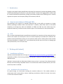
1 Introduction
During the last decade various quantification techniques for proteomics have been developed including
stable isotope labelling of amino acids in cell culture (SILAC)1, tandem mass tagging (TMT)2, isobaric tags
for relative and absolute quantification (iTRAQ)3 and isobaric peptide termini labelling (IPTL)4. IsobariQ
supports the reporter ion techniques (iTRAQ, TMT and others) and IPTL.
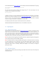
1.1 Reporter ion techniques (iTRAQ and TMT)
The advantage of the reporter ion methods iTRAQ and TMT is their ability to compare up to eight
different physiologic conditions within one experiment5. In addition, unlike SILAC, there is no increased
complexity at the MS level, while the drawbacks of iTRAQ and TMT are their relative high cost,
systematic dampening6 and that the low molecular region is not accessible to all mass spectrometers.
1.2 IPTL
IPTL is a recently developed isobaric quantification method for the comparison of two proteomes that is
similar to the reporter ion techniques in that no increased complexity at the MS level is obtained. IPTL
produces several quantification points per mass spectrum which yields a robust and accurate estimate
of protein abundances. In addition, IPTL is not hampered by the low mass cut-off seen in trapping type
mass spectrometers, such as LTQ ion traps.
2 Working with IsobariQ
2.1 Installation and licence
IsobariQ can be downloaded free of charge at www.biotek.uio.no/research/thiede_group/software and
unpacked to a folder of choice using standard archiving tools. IsobariQ is started by double-clicking the
IsobariQ.exe file.
IsobariQ is licensed under the GNU General Public Licence version 3, and parts of the software (mainly
libraries) are licensed using compatible licences. To view all licences and the external libraries, click F4 or
see the help menu in IsobariQ.
2.1.1 Installation of R, vsn and Rserve
For optimal usage, we recommend installing the statistical software R7. This enables IsobariQ to
communicate with R and perform variance stabilizing normalization (VSN) of the data. See section
2.3.2.2 of this manual for details.
4
R can be downloaded from www.r-project.org. Once installed, run R and install Bioconductor 8 by typing:
source("http://bioconductor.org/biocLite.R")
biocLite()
This will install several necessary packages, and amongst them vsn9 . If, for some reason, vsn is not
installed it can be installed with the command:
biocLite(“vsn”)
In addition to R and vsn, you have to download and install a frontend server called Rserve. For Windows,
download the stand-alone windows binary from www.rforge.net/Rserve/files and unpack this into a
directory of choice. The executable Rserve.exe needs to be copied to the ‘/bin’ folder of R (usually
located in C:/Program Files/R) due to its dependence on the file R.dll.
For IsobariQ to perform VSN, the path to Rserve needs to be set in preferences.
IsobariQ was developed and tested with R version 2.11.1 and Rserve version 0.6-2.
2.2 Importing Data
2.2.1 Supported File Formats
IsobariQ supports data generated by Mascot10 (www.matrixscience.com). Mascot is a proteomics search
engine that uses mass spectrometry data to identify proteins from primary sequence databases, and
access to the Mascot dat-files is required. Mascot stores its search results in a text based file located on
the mascot server (usually in the folder C:/INETPUB/MASCOT/data/yyyymmdd). We recommend
copying these dat-files locally before importing to IsobariQ for performance reasons.
Note: Only Mascot dat-files originating from MS/MS searches are supported. Peptide mass fingerprints
or error tolerant searches cannot be loaded in IsobariQ.
Note: If the Mascot dat-files are large (>200 MB), importing them in IsobariQ may be time consuming.
To improve loading time one can apply filters. See ‘Data Import Wizard’ below for details. IsobariQ
stores the search results in memory while loading, and if >2 GB of RAM is used it may close
unexpectedly (32bit version of IsobariQ). IsobariQ was designed to use memory for storage for
performance reasons.
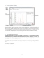
2.2.2 Data Import Wizard
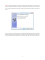
Importing data into IsobariQ is done by selecting ‘Import Data’ from the ‘File’-menu. This will open the
‘Data Import Wizard’.
5
Note: Not all settings applied in the wizard can be changed after data loading. These settings will be
visible in preferences, but disabled. To change one of these parameters, the data has to be re-imported.
This is because the parameters define how IsobariQ should read the Mascot dat-files and treat the
results.
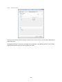
In the first frame the user chooses the kind of quantification technique that was used in the study. Two
techniques are supported, IPTL and Reporter Ions. Under ‘IPTL’ the methods ‘Standard IPTL’ and ‘Tryptic
IPTL’ are supported, and under ‘Reporter Ions’ the methods ‘iTRAQ’, ‘TMT’ and ‘Custom’ are supported.
6
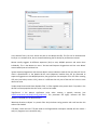
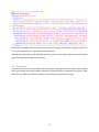
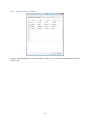
In the Mascot frame, the user selects the path to the Mascot dat-file. This file can be located either
locally or on a network drive, but we recommend having the file locally for performance reasons.
Mascot usually suggests 10 different sequences (hits) to every MS/MS spectrum and scores them
individually. This is the Mascot ion score. ‘Do Not Load Sequence Suggestions with Ion score Below’
causes IsobariQ not to load these hits.
‘Ignore Sequence Suggestions with Ionscore Below’ causes IsobariQ to load the hits, but they will not be
used in quantification. In the detailed Q-IPTL and Q-Reporter modules they will be presented as
sequence suggestions to the MS/MS spectrum, but greyed out. One exception is for IPTL when creating
IPTL pairs (see below, section 2.2.3), where it is sufficient that only one of the two hits have ion score
above this value.
‘Do Not Load Proteins with Fewer Peptides Than’ is a filter applied at the protein level. If a protein in the
dat-file has fewer peptides than this value, it will not be loaded.
‘Significance’ is the Mascot significance value when creating a peptide summary (see
www.matrixscience.com/help/scoring_help.html). This parameter will highly influence the false
discovery rate (FDR) for the identifications.
‘Maximum Proteins to Report’ is a protein filter. Only the best scoring proteins with rank less than this
value will be loaded.
‘ETD data’. Check this box if ETD was used as the fragmentation technique. IsobariQ will then match c
and (z+1) fragment ions instead of b and y.
7
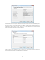
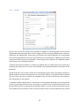
‘Standard IPTL’ refers to the original published method4 which includes cross-wise peptide labelling of Nterminals and lysines. This technique requires a Lys-C digest, causing relatively long peptides where ETD
fragmentation might be superior to CID. ‘Tryptic IPTL’ is a novel derivative of this method utilizing
trypsin as the protease and specific C-terminal labelling.
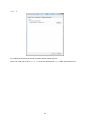
Using the reporter ions technique, the user can select from a set of preset methods or choose the
number of reporters manually. Up to eight reporters are supported.
8
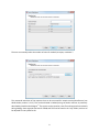
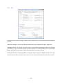
The user can manually select the number of ratios for IsobariQ to report, maximum 7.
The measured intensities of the reporters have to be corrected for isotopic overlap/interference (see
details below, section 2.3.1.2). This can be achieved in IsobariQ using correction matrices as previously
described by Vaudel and colleagues11. The matrix can be stored in a text file and imported into IsobariQ
during loading. Some example matrices for iTRAQ and TMT can be found in the ‘conf’ folder, but have to
be adjusted for every different kit.
9
2.2.3 Filtering of Mascot Results and Identification of IPTL Labelling
Mascot usually suggests 10 sequences (hits) for each MS/MS spectrum and ranks them according to
their ion score. Which of the sequences Mascot uses depends on the protein context. If a hit falls below
the ion score cut off set by the user while loading data, the hit is not loaded. If the removed hit was the
one used by Mascot for this protein, the peptide will not show as a part of the protein and the protein
score is recalculated.
If Mascot suggests a sequence that is labelled according to the selected IPTL labels, for example Nterminally succinylated (light) and the C-terminal lysine being labelled with MDHI (heavy), then this hit is
marked as IPTL-labelled. When all hits have been checked for IPTL-labelling, IPTL pairs will be created if
they have matching sequences, but opposite IPTL labels (succinylated (heavy) and MDHI (light)). This will
only occur, however, if this is the sequence Mascot uses for this peptide.
Special IPTL Feature: If in a peptide Mascot cannot identify the reverse sequence, i. e., only identified in
one direction in Mascot, IsobariQ will try to “force-find” the opposite sequence. If this sequence is found
in the MS/MS spectrum and produces a number of valid ratios to be calculated (this value can be set in
the import wizard) this hit is stored as force-found, and an IPTL pair is generated.
Only MS/MS spectra with IPTL pair identifications can be quantified.
For reporter ion quantification, all MS/MS spectra with detected reporters can be quantified.
Whether a peptide can be quantified or not is annotated in the table by a green tick-mark or a red X,
respectively. Peptides that are quantifiable due to the above described “force-found” method are
annotated with an orange tick-mark.
2.3 Quantification, Normalisation and Significance
The workflow of computations in IsobariQ is as follows:
i.
Quantify each peptide individually.
For IPTL, this means quantifying each fragment pair individually and calculating a peptide
median and peptide variability. For reporter ions, this means correcting the measured intensities
with the correction matrix, and calculating the different ratios between the reporters. All at the
MS/MS level.
ii.
Normalise the peptide ratios.
Normalisation corrects for unequal loading and experimental error that causes the overall
distribution of ratios to deviate from 1:1. Normalisation assumes that the majority of ratios
should be 1:1. One special algorithm for normalisation is the variance stabilising normalisation
(VSN) which also reduce the variance heterogeneity found in proteomics data12.
iii.
Quantify each protein individually.
10
This means calculating an overall protein ratio based on all the peptides found for that protein.
iv.
Perform statistical tests.
Use the overall distribution of protein ratios to calculate individual protein significance using zstatistics, and compute limits for up- and down-regulated proteins.
2.3.1
Calculation of Peptide Ratios and Variability
2.3.1.1 IPTL
In IPTL, a peptide can have several quantification points, and they are based on the identification by
Mascot. IPTL pair identifications consist of pairs of sequence fragments, for example y5 and y’5; one
belonging to the first IPTL labelling group and the other to the second labelling group. When a pair has
been found the ratio to use depends on the labelling of the peptide, whether the fragment is a b or y (or
c or (z+1)) and finally the user’s selections whether the ratio should be reported as control/treated or
treated/control.
Example:
The control experiment is labelled with light labelled N-terminals and we want to report the ratio as
treated/control. The fragment to consider is b6 and the associated sequence is heavy N-terminally
labelled.
b-fragments are N-terminal fragments, meaning that this is a fragment with a heavy label and
originating from the treated sample. b’6 is then the counter fragment originating from the control. The
correct ratio to use would then be b6/b’6, or heavy/light.
For y6, it would have been a C-terminal fragment with a light label. The counter fragment, y’6, would
then be from the control and have the heavy label. The ratio to use would still be y6/y’6, but then
light/heavy.
The ratio is calculated using the intensities of the ions.
If an ion can be assigned to more than one sequence fragment, then it will not be used for quantification.
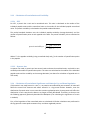
The peptide ratio is calculated as the median of all the ion ratios and the variability as the average
deviation in log-space. Standard deviation was not chosen to describe the statistical dispersion due to its
utilisation of the mean and not the median as the central tendency. The average deviation is defined as:
11
Where M is the median of the log-transformed ratios and x is the log-transformed ratio.
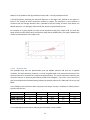
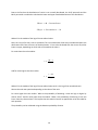
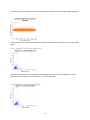
A second parameter describing the statistical dispersion is the angle score, defined as the slope of a
linear fit line through all ratios sorted from smallest to largest. This parameter is more sensitive to
variations than the average deviation and is intended to ease the finding of outlier ratios within one
MS/MS spectrum. It is also highly influenced by the number of quantification points.
For example, for a given peptide 15 ratios can be calculated varying from 1.09 to 2.98. The ratio plot
below shows the ratios (black dots), the fitted line (red) and the median (blue). The angle θ between the
median and the fitted line is the angle score.
2.3.1.2 Reporter Ions
This technique only uses one quantification point per MS/MS spectrum and thus has no peptide
variability. The ratio calculation, however, is still not straightforward as the measured intensities of the
reporters have to be corrected for isotopic overlap/interference. This can be achieved in IsobariQ using
correction matrices as previously described by Vaudel and colleagues11. The matrix can be stored in a
text file and imported into IsobariQ during loading. See example matrices for iTRAQ and TMT in the ‘conf’
folder.
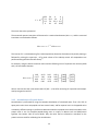
In the iTRAQ-kit the information about impurities and isotopic overlap is included. For iTRAQ 4-plex it
typically looks like this:
Reagent
iTRAQ®-4plex 114
iTRAQ®-4plex 115
iTRAQ®-4plex 116
iTRAQ®-4plex 117
% of -2
0
0
0
0
% of -1
1.0
2.0
3.0
4.0
% of 0
92.9
92.9
92.4
92.4
% of +1
5.9
5.6
4.5
3.5
A corresponding correction matrix reflecting this information can be created:
12
% of +2
0.2
0.1
0.1
0.1
The matrix has to be symmetrical.
The measured reporter intensities will be stored in a matrix when detected, Mmeasured, and the corrected
intensities are calculated as follows:
The inverse of C is calculated using first LU decomposition (Gaussian elimination with partial pivoting13)
followed by solving the system Ax = b for each column of the identity matrix. All computations are
performed using the GNU Scientific library14.
For example, using the above correction matrix and the following 114-117 reporters with intensity 1000
each, the calculations become:
We can now see that the uncorrected ratio 115/114 = 1, but after correcting for impurities and isotopic
overlap we get the ratio 0.9.
2.3.2 Normalisation of Peptide Ratios
Normalisation is performed by using the complete distribution of calculated ratios. That is for IPTL all
quant point ratios since one peptide can have several ratios, and for reporter ions it is the peptide ratios.
In IsobariQ, different settings in preferences determine whether a peptide ratio should contribute to the
protein ratio or not. For example peptide being razor or unique, or Mascot rank and bold/normal
typeface. See section 2.8.1 for more details. Only the ratios that are selected to contribute to the
protein ratio are used for calculating the normalisation.
13
In IsobariQ the user can choose between:
1.
2.
3.
4.
No Normalisation
Division by Median
Variance Stabilising Normalisation
Division by Channel Sum (Reporter Ions Only)
The results of the normalisation can be validated using different graphs. See section 2.4 for more details.
2.3.2.1 Division by Median
Normalization is performed by utilising the ratios of all peptides (Reporter Ions) or quant points (IPTL).
The normalised peptide / quant point ratio is calculated as follows:
Where M is the median of all peptides / quant points.
2.3.2.2 Variance Stabilising Normalisation
For details about VSN, see previously reported data for iTRAQ9, or visit the homepage at
www.bioconductor.org/packages/devel/bioc/html/vsn.html. In brief, VSN transforms the distribution of
signal intensities in order to stabilise the variance across the whole intensity range. The phenomenon
usually seen in proteomic experiments is called heterogeneity of variance and is the dependence of the
ratio on the mean signal. It can be seen as a wider spread of ratios in the low-intense region in a
distribution plot of ratios, when compared to the high-intense region.
2.3.2.3 Division by Channel Sum (Reporter Ions Only)
For each reporter (channel) the sum of all intensities are calculated, and a normalised reporter intensity
for the 114 channel of iTRAQ would be calculated as follows:
Where I is measured intensity (or rather the corrected intensity if a correction matrix is used) and S is
the channel sum of all intensities.
The ratios are then calculated using the normalised intensities.
14
2.3.3
Calculation of Protein Ratios and Variability
2.3.3.1 IPTL
For IPTL, a protein has a ratio and a normalised ratio. This ratio is calculated as the median of the
individual peptide ratios and the normalised ratio as the median of the individual peptide normalised
ratios. The protein variability is calculated as the pooled standard deviation.
The pooled standard deviation uses the individual peptide variability (average deviation) and the
number of quantification points in each peptide as the basis. The protein variability is then calculated as
follows:
Where V is the peptide variability (using normalised data) and Q is the number of quantification points
in the peptide.
2.3.3.2 Reporter Ions
In reporter ion mode, a protein can have several ratios and several normalised ratios; each with its own
variability and number of quantification points. The ratios are calculated as the median of the individual
peptide ratios and the variability as the average deviation (see above for calculation of peptide ratio in
IPTL mode).
2.3.4 Calculation of Protein Ratio Significance and Limits for Up- and Down Regulation
If all proteins in our study have a 1:1 ratio, i.e., no proteins were affected by our treatment, all ratios will
follow the central limit theorem and scatter around 1 in a log-normal fashion. However, since the
distribution of protein ratios in most cases also contain regulated proteins, these proteins will affect the
distribution in such a way that the data are no longer normally distributed. Therefore, we chose to use
the following approach (previously described for MaxQuant15) for calculating the significance of a ratio
in IsobariQ:
First, all the logarithms of the normalised ratios are calculated. All further calculations are performed in
this log-space to ensure equal treatment of up- and down-regulated proteins.
15
Due to the fact that the distribution of ratios is not normally distributed, the 15.87 percentile and the
84.13 percentile are utilised to calculate the lower and upper standard deviations of the distribution.
Where M is the median of the log of the normalised ratios.
Next, the z-score for every ratio is calculated. The z-score describes ‘how many standard deviations the
observation falls from the centre of the distribution’. It has to be calculated with the correct SD, either
lower or upper, depending on which side of the median the ratio is.
For ratios lower than the median:
And for ratios higher than the median:
Where M is the median of the log of the normalised ratios and r is the log of the normalised ratio.
We can then ask two questions depending on the value of the ratio:
For ratios higher than the median: ’What is the probability of obtaining a ratio this high or higher by
chance alone?’ And for ratios lower than the median: ’What is the probability of obtaining a ratio this
low or lower by chance alone?’ This implies that the statistical test to be applied has to be one-sided for
each question.
The probability can be calculated using the Gaussian probability function
16
which returns the upper tail of the distribution. Since the test is one-sided for each question, the values
obtained will range from 0 to 0.5. The significance level is up to the user, but IsobariQ calculates the
limits shown in the distribution graph at α = 0.05. These limits can easily be calculated as follows:
Where M is the median of the log of the normalised ratios. These limits are now in log-space and need
to be transformed before applied to ratios. The constant 1.645 is the z-score from the normal
probability table that ensures 5% probability.
2.4 Graphs
Many different graphs exist, depending on quantification mode selected. Original data is shown in blue,
while normalised data is shown in orange. By right-clicking in the graph the image can be copied or
saved. The XY-data can also be retrieved for pasting into any spread sheet application and further
plotting.
Here the graphs are explained briefly.
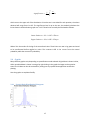
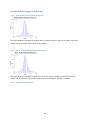
2.4.1
Protein Ratio Distribution Histogram
17
This graph shows the histogram of protein ratios.
2.4.2
Peptide Ratio Distribution Histogram
This graph shows the histogram of peptide ratios. It should be similar to the one for protein ratios, but
usually contains more data points and thus is smoother.
2.4.3
Quant Point Ratio Distribution Histogram
This graph shows the histogram of quant point ratios (IPTL only). It should be similar to the one for
protein and peptide ratios, but usually contain even more data points and thus is smoother.
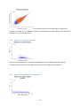
2.4.4
Quant Point Intensities
18
This graph shows all the quant points (IPTL only) plotted control versus treated. Blue is original and
orange is normalised. The 1:1 regulation is shown as a black dotted line. VSN transforms the distribution,
especially for low intense data points.
2.4.5
Peptide CV vs. Peptide Intensity
Graph to see if the peptide CV is related to the peptide intensity. The peptide intensity is not the
precursor intensity, but the sum of fragment intensities that are assigned to the sequence.
2.4.6
Peptide CV vs. Rank of Peptide Intensity
19
Often it is useful to plot versus the rank of intensities instead of the intensity itself. From this graph one
can easily conclude that the CV seems homogeneous for all peptide intensities, i.e., it is not linked to the
peptide intensity (It is a bit more difficult to get to that conclusion in the previous graph).
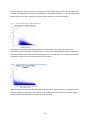
2.4.7
Quant Point CV vs. Mean Intensity
Quant point CV is something completely different from peptide CV. The quant point is one ratio
calculated from two intensities. The quant point CV is here the CV calculated from these two intensities.
The mean intensity is the mean of these two intensities. So in this plot the CV, or variance, between two
intensities are larger for low intense data than for high intense.
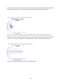
2.4.8
Quant Point CV vs. Rank of Mean Intensity
When the same (see previous graph) is plotted versus the rank of mean intensities, it is evident that the
variance is higher for low intense, but actually for the 25 000 most intense points the variance is quite
stable already. Performing VSN on this data set yields this graph:
20
The bulk of the data is not transformed, only the first 5000 data points. But now the variance is stable
across the whole intensity range.
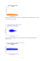
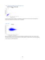
2.4.9
Quant Point Ratio vs. Mean Intensity
Graph to see the spread of quant point ratios as a function of mean intensity (described above).
Identical to 2.4.16.
2.4.10 Quant Point Ratio vs. Rank of Mean Intensity
21
As previous, just plotted against the rank of mean intensity. A VSN version of this data yields this graph:
Here we can see that for low intense data the statistical spread of ratios are lower than the original data
above.
2.4.11 Peptide CV vs. Peptide Angle Score
Plot to see if the peptide CV is comparable / proportional to our own metric, the angle score. Graph
shows that the two metrics are not the same, i.e., none is redundant.
2.4.12 Peptide CV vs. Peptide Variability
22
Plot to see if the peptide CV is comparable / proportional to the peptide variability (average deviation).
The peptide CV takes into account the peptide ratio, while the peptide variability does not.
2.4.13 Peptide Intensity vs. Peptide Variability
Plot to see if the peptide variability is linked to peptide intensity. Note that the peptide intensity is
different to the mean intensity used before (see 2.4.7). The peptide intensity is the intensity calculated
as the intensity sum of the fragments in the MS/MS spectrum that are assigned to the sequence.
2.4.14 Peptide Ratio vs. Rank of Peptide Intensity
Plot to see relation between peptide ratio and peptide intensity.
23
2.4.15 Peptide Variability vs. Peptide Angle Score
Plot to see if the peptide variability is comparable / proportional to our own metric, the angle score.
Graph shows that the two correlate, but are not identical.
2.4.16 M-A
Minus vs. Add plot. Used to look for intensity-dependent trends (banana shape). M is the quant point
ratio while A becomes the average intensity for a ratio. Actually, it is identical to 2.4.9, but kept separate
in the list due to its well known name.
24
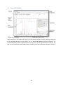
2.5 The Q-IPTL Module
When IsobariQ is in IPTL-mode and a protein has been double-clicked, the Q-IPTL module will open and
all the peptides belonging to that protein can be viewed and validated. Detailed information like
annotated MS/MS spectrum, possible sequence matches, IPTL pairs and quantification is available. The
user can interact with the quantification events, something that causes IsobariQ to recalculate on the fly.
25
2.6 The Q-Reporter Module
When IsobariQ is in Reporter-mode and a protein has been double-clicked, the Q-Reporter module will
open and all the peptides belonging to that protein can be viewed and validated. Detailed information
like annotated MS/MS spectrum, possible sequence matches and quantification is available. The user
can interact with the quantification events, something that causes IsobariQ to recalculate on the fly.
2.7 Saving and Exporting Data
IsobariQ saves all the data in its own format, QXML. This format stores all the experiment information
(settings, peptide/protein identification and quantification) and all the user interactions. In this way, the
user can go back to old data and continue validation at a later time point. The QXML format is an XML
based format which is also readable for humans.
IsobariQ does not support mzIdentML at this point; mainly due to its lack of support for quantification
data.
One example of a QXML file:
26
Please note that A LOT of data is saved, and this process may take time. However, loading of QXML files
is very quick compared to re-importing the Mascot dat-files.
IsobariQ also exports data as tab separated text files (tsv-files). These can be imported into spread sheet
applications like Excel for downstream analysis.
2.8 Preferences
In preferences the user can view settings selected during the loading of data (in the Data Import Wizard)
and access settings that affect program behaviour and quantification of peptides and proteins. After
alterations in preferences, all data should be re-quantified to incorporate the changes.
27
2.8.1
General
Here the user can set the scoring schema (standard or MudPIT for calculating protein scores) and the
fragmentation techniques (ETD: uses c and (z+1) fragments when annotating MS/MS spectra). Leave unchecked for CID fragmentation. Furthermore, the threshold for matching fragment ions at the MS/MS
level can be set (typically 0.6 Da for ion traps and lower for TOF instruments). In addition there are a few
settings that affect the protein quantification. These settings will be applied to the individual peptides
when the user clicks ‘Quantify all proteins’.
If ‘Require bold red (from Mascot)’ is checked, any peptide that is not bold red will not be used when
calculating the protein ratio. In the main view of IsobariQ, the peptide quantification information will be
greyed out.
Peptide uniqueness can be used as a filter when calculating the protein ratios. The peptide is unique if a
peptide sequence has been associated with only one protein in Mascot. If a peptide has been associated
with more than one protein in Mascot, but assigned to only one due to the Occams razor principle16,
then the peptide is a razor peptide.
If ‘Normalize rawfiles independently’ is checked, then all the peptides identified will be normalised per
raw file. For gel-experiments this can be very useful, as a protein can be identified many places on the
gel with different ratios, for example due to cleavage. However, a certain amount of data points per raw
file is needed for correct statistics, so do not use this option if there are only few data points per raw file.
28
2.8.2
IPTL
These are the IPTL specific settings; however most of them are set in the Import Data Wizard (greyed
out here).
‘Label mass difference’ is the mass difference between the heavy and light IPTL labels, usually 4 Da.
IsobariQ generates “force-found” hits when Mascot cannot detect both forward and reverse labelling
(see section 2.2.3). The minimal number of ratios required is set during loading in the Import Data
Wizard, but whether to use them for protein quantification or not can be set here.
IPTL allows two states to be compared. One is assumed ‘Control’ and one ‘Treated’; however, this is just
nomenclature and does not have to be the case. Here you can set how IsobariQ should report the ratios.
29
2.8.3
Reporter ions
These are the reporter specific settings; however most of them are set in the Import Data Wizard
(greyed out here).
The ‘MS/MS tolerance’ is the match threshold for the reporters in the MS/MS spectrum. This is usually
high resolution data and can be set low (typically at 0.1 Da).
30
2.8.4
Reporter Correction Matrix
Here the computed Reporter Correction Matrix is shown. It is the inverse of the loaded text file (see
section 2.2.2).
31
2.8.5
R
For IsobariQ to communicate with R the path to Rserve needs to be set.
Note: This is the path to the Rserve.exe that was copied to the R/bin folder (see section 2.1.1).
32
3 References
1.
2.
3.
4.
5.
6.
7.
8.
9.
10.
11.
12.
13.
14.
15.
16.
Ong, S. E.; Blagoev, B.; Kratchmarova, I.; Kristensen, D. B.; Steen, H.; Pandey, A.; Mann, M.,
Stable isotope labeling by amino acids in cell culture, SILAC, as a simple and accurate approach
to expression proteomics. Mol Cell Proteomics 2002, 1, (5), 376-86.
Thompson, A.; Schafer, J.; Kuhn, K.; Kienle, S.; Schwarz, J.; Schmidt, G.; Neumann, T.; Johnstone,
R.; Mohammed, A. K.; Hamon, C., Tandem mass tags: a novel quantification strategy for
comparative analysis of complex protein mixtures by MS/MS. Anal Chem 2003, 75, (8), 1895-904.
Ross, P. L.; Huang, Y. N.; Marchese, J. N.; Williamson, B.; Parker, K.; Hattan, S.; Khainovski, N.;
Pillai, S.; Dey, S.; Daniels, S.; Purkayastha, S.; Juhasz, P.; Martin, S.; Bartlet-Jones, M.; He, F.;
Jacobson, A.; Pappin, D. J., Multiplexed protein quantitation in Saccharomyces cerevisiae using
amine-reactive isobaric tagging reagents. Mol Cell Proteomics 2004, 3, (12), 1154-69.
Koehler, C. J.; Strozynski, M.; Kozielski, F.; Treumann, A.; Thiede, B., Isobaric peptide termini
labeling for MS/MS-based quantitative proteomics. J Proteome Res 2009, 8, (9), 4333-41.
Choe, L.; D'Ascenzo, M.; Relkin, N. R.; Pappin, D.; Ross, P.; Williamson, B.; Guertin, S.; Pribil, P.;
Lee, K. H., 8-plex quantitation of changes in cerebrospinal fluid protein expression in subjects
undergoing intravenous immunoglobulin treatment for Alzheimer's disease. Proteomics 2007, 7,
(20), 3651-60.
Ow, S. Y.; Salim, M.; Noirel, J.; Evans, C.; Rehman, I.; Wright, P. C., iTRAQ underestimation in
simple and complex mixtures: "the good, the bad and the ugly". J Proteome Res 2009, 8, (11),
5347-55.
R-Development-Core-Team R: A Language and Environment for Statistical Computing.
http://www.R-project.org (2010),
Gentleman, R. C.; Carey, V. J.; Bates, D. M.; Bolstad, B.; Dettling, M.; Dudoit, S.; Ellis, B.; Gautier,
L.; Ge, Y.; Gentry, J.; Hornik, K.; Hothorn, T.; Huber, W.; Iacus, S.; Irizarry, R.; Leisch, F.; Li, C.;
Maechler, M.; Rossini, A. J.; Sawitzki, G.; Smith, C.; Smyth, G.; Tierney, L.; Yang, J. Y.; Zhang, J.,
Bioconductor: open software development for computational biology and bioinformatics.
Genome Biol 2004, 5, (10), R80.
Huber, W.; von Heydebreck, A.; Sultmann, H.; Poustka, A.; Vingron, M., Variance stabilization
applied to microarray data calibration and to the quantification of differential expression.
Bioinformatics 2002, 18 Suppl 1, S96-104.
Perkins, D. N.; Pappin, D. J.; Creasy, D. M.; Cottrell, J. S., Probability-based protein identification
by searching sequence databases using mass spectrometry data. Electrophoresis 1999, 20, (18),
3551-67.
Vaudel, M.; Sickmann, A.; Martens, L., Peptide and protein quantification: a map of the
minefield. Proteomics 2010, 10, (4), 650-70.
Karp, N. A.; Huber, W.; Sadowski, P. G.; Charles, P. D.; Hester, S. V.; Lilley, K. S., Addressing
accuracy and precision issues in iTRAQ quantitation. Mol Cell Proteomics.
Golub, G. H.; Van Loan, C. F., Matrix computations. 3rd ed.; Johns Hopkins University Press:
Baltimore, 1996; p xxvii, 694 p.
Galassi, M., GNU scientific library : reference manual. 2nd ed.; Network Theory: Bristol, 2002; p
xvi, 601 p.
Cox, J.; Mann, M., MaxQuant enables high peptide identification rates, individualized p.p.b.range mass accuracies and proteome-wide protein quantification. Nat Biotechnol 2008, 26, (12),
1367-72.
Nesvizhskii, A. I.; Aebersold, R., Interpretation of shotgun proteomic data: the protein inference
problem. Mol Cell Proteomics 2005, 4, (10), 1419-40.
33