1
Proline Suite
User Guide
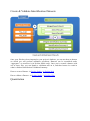
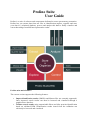
Proline is a suite of software and components dedicated to mass spectrometry proteomics.
Proline lets you extract data from raw files or identification engines, organize and store
your data in a relational database, process and analyse this data to finally visualize and
extract knowledge from MS based proteomics results.
Proline suite main features
The current version supports the following features:
Import identification results (OMSSA and Mascot files are currently supported).
Once imported, search results can then be browsed and visualized through a
graphical user interface.
Validate search results using customizable filters and infer proteins identification
based on validated PSM. Identification results issued from the validation can
obviously be browsed and visualized.
Combine individual search results or identification results to build a
comprehensive proteome.
Export identification results in different formats including standard exchange
formats.
The software suite is based on three main components:
A relational database management system storing the data used by the software
in four different databases
A web server handling processing tasks and web data access
Two different graphical user interfaces, both allowing users to launch tasks and
visualize their data: Proline Studio which is a rich client interface and Proline
Web the web client interface
An additional component is used by administrators to setup and manage Proline (called
ProlineAdmin).
Setup and Install
Read the Installation & Setup documentation to install, start the different modules used by
Proline or upgrade your installation with a newer version
Getting Started
Discover Proline's workflow and how to execute it with Proline Studio and Proline Web.
How-to
Find quick answer to your questions in this How to section.
Concepts
Read the Concepts & Principles documentation to understand main concepts and
algorithms used in Proline.
Releases
Both interfaces, Studio and Web, are based on a set of databases.
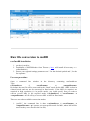
Raw file conversion to mzDB
This procedure is detailed in the mzDB Documentation section.
Installation & Setup
This page gives you a short overview of Proline components architecture and explains how
to install and setup the different components
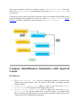
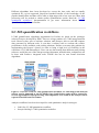
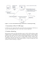
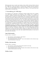
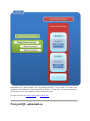
Architecture Overview
The suite is based on different components (see figure below):
A Relational Database Management System (Proline Datastore) storing the data
used by the software in different databases.
A web server (Proline Server) handling processing tasks and web data access
Two different graphical user interfaces, both allowing users to launch tasks and
visualize their data:
o ProlineStudio which is a rich client interface
o ProlineWeb the web client interface
A daemon application, Proline Sequence Repository, automaltically filling
proteins sequences repository from fasta.
A system administration application (ProlineAdmin) to setup and manage the
Proline suite. This application is available as a command line applicatin or with a
graphical user interfaces.
Proline components
Proline DataStore
Proline stores data in six different database schemas. Three of them are “core” database
schemas created once at datastore initialization. This three databases contains data related
to users projects (UDS database), peptides sequences and post-translational modifications
(PS database) and proteins and databank (PDI database). The Seq database, where
protein ID and sequence are store, is automatically created when running the associated
daemon application (Sequence Repository). This database is needed to have protein
sequences and descriptions in user interfaces. The PDI database (with more information
than the sequence database) is not available yet.
The two additional schemas are used to create a new database each time you create a new
user project. This databases store identification data (MSI databases) and quantification
data (LCMS database) associated with users projects.
Requirements
The server-centric architecture of Proline imposes different requirements for the server
computer and the client computers.
Server-side Proline requirements:
o a Java SE 8 JRE or above must be installed.
o the PostgreSQL database server (tested versions are 9.X) must be installed
and configured. On windows the automated installer includes the
PostgreSQL server, which can be installed on the same computer than
Proline or a dinstinct one. By default, PostgreSQL settings are defined for
modest hardware configurations but they can be modified to target more
efficient hardware configurations (See PostgreSQL optimization).
o Proline-Server must run in English “locale”, on Linux OS, environment
variable LANG=en_US.UTF-8 can be exported before starting ProlineWebCore. If not in english, you can also modify the jetty.runner.sh (see
installation steps) to add -Duser.language=“en” -Duser.country=“US”
parameters
Client-side requirements for Proline Studio:
o a Java SE 7 JRE or above must be installed (on Windows OS, ProlineStudio installer already includes a JRE 32 or 64-bit distribution)
If you want to use Proline remotely through a Web client, the ProlineWeb components and
their requirements must also must installed.
Server-side ProlineWeb requirements:
o MongoDB database server must be installed. Note: this database server can
be installed on a distinct computer.
Client-side requirements for Proline Web:
o a recent Web Browser (IE 9+, Firefox 25+, Chrome 30+).
Installing Proline Suite
To install Proline for the first time, go here
Installing the Proline Suite
The Proline suite is based on (different components). The following documentation
describes the installation procedure for each of this component:
Proline server
Sequence Repository
Proline Studio
Proline Web
Proline server installation and setup
Proline server installation
Windows users
Download
the
automated
installer
(http://proline.profiproteomics.fr/download/).
from
the
Proline
website
The
wizard
will
guide
you
through
the
installation
process.
By default, the installer will unpack all components on the computer. However, it is
possible to install the Proline components on distinct computers if it fits better your
hardware architecture.
For users who prefer manual installation or witout administrator rights, an archive file
of the distribution is also available. You can follow the installation procedure described in
the next section.
Linux users or manual installation
There is no automated installer at the moment.
First check that all requirements are first installed on the computer.
Then download the zip archive containing Proline components from the dedicated website
(http://proline.profiproteomics.fr/download/).
The Proline Server archive file contains three others archives corresponding to the
(different components).
Proline WebCore : the Proline Server
Proline Admin GUI
Sequence Repository
Unzip these components on the appropriated computer (Proline Server and Proline Admin
is recommanded to be on the same computer. Sequence Repository is recommanded to be
installed on the computer where fasta files are accessible)
Once Proline is installed you must initialize Proline datastores and settings.
On this purpose, the Proline-Admin software is provided with the Proline Suite. It is
available as a command-line tool or as Graphical Interface called Proline-Admin GUI.
We will guide you through this process, step by step, using both these tools.
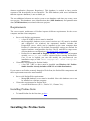
Setting up the Datastore
You must first configure ProlineAdmin since this component is used to create the
databases needed by Proline.
From graphical tool ProlineAdmin GUI
Launch ProlineAdmin GUI
Windows users
A shortcut “Proline Admin” is available in the Windows Start Menu, under the Proline
folder.
Linux users or manual installation
Execute the start.sh script located in the folder obtained after Proline Admin GUI
archive file extraction.
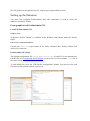
ProlineAdmin GUI usage
The default configuration file config/application.conf is loaded. You can alternatively
edit this file (see Configuring ProlineAdmin section below) or select another .conf file of
the same format.
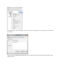
To edit default file, press the “Edit Proline configuration” button. You can now edit your
file in the newly opened window, and save it.
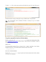
To load a .conf file, use the menu on the top left and select your file in the file browser.
Finish the datastore setup by clicking the newly available button “Set up Proline”.
Note: This functionnality will be disabled if Proline is already set up or if Proline
configuration is invalid.
Using the command line interface (ProlineAdmin)
Edit the configuration file config/application.conf located in the ProlineAdmin folder
(see Configuring ProlineAdmin section below). Then perform the datastore setup by
running the dedicated script.
Windows users
The ProlineAdmin program files are located in the “.\admin” sub-folder of the Proline
installation directory. You should find the following script in this folder:
> setup_proline.bat
Linux users or manual installation
Execute the setup_proline.sh script located in the folder obtained after Proline Admin
GUI archive file extraction.
Configuring ProlineAdmin
Modify the following lines to fit your DBMS configuration:
proline-config {
driver-type = "postgresql" // valid values are: h2, postgresql or sqlite
data-directory = "/Path/to/Proline/Data" //Not used actually...
}
auth-config {
user="proline_user" // !! SET TO Database Proline user login
password="proline_user_password" // !! SET TO Database Proline user
password
}
host-config {
host="your_postgresql_server_host" //!! Do NOT put "localhost", but the
real IP address or fully qualified name
port="5432" //or other port used to access your DBMS
}
Note: default naming scheme of databases created by Proline can be modified by editing
config/application-<dbtype>.conf file.
Configuring the Proline Server
Locating the server folder
Windows users
The server program files are located in the “.\ws” sub-folder of the Proline installation
directory.
Linux users or manual installation
Open the folder where you have unzipped the “Proline Server” archive. The Proline server
folder should contain a sub-folder named ProlineWeb-Core-<x.y.z>.
Editing the configuration file
The configuration file is located at <proline_server_folder>\ProlineWeb-Core<x.y.z>\Proline\WEB-INF\classes.
Configuring the datastore
Edit the application.conf file in the same way you did it for ProlineAdmin (see Setting
up the Datastore). If your configuration is valid, the Proline Server will be able to use the
datastore you've created using Proline Admin.
Configuring the mount-points
Result identification files (Mascot dat or OMSSA) as well as mzDB files (for the XIC
Quantitation process) are only browsed from Proline Server side.
Administrator must configure the target directory/ies in the entry mount_points in the
application.conf file
Mascot dat or OMSSA path should be configured in result_files sub-entry,
administrator
can
add
one
or
more
mappings
as
label
=
“<absolute/directory/path>”. mzDB files path should be set under mzdb_files subentry.
Label can be any valid string chosen by Administrator to help user identify mount_point. If
multiple repositories are defined, labels must be different.
Configuration examples:
mount_points {
result_files {
mascot_data = "Z:/" //under window environement
omssa_data = "/local/omssa/data" //under linux environement
...
}
...
mzdb_files {
}
}
Running the server
Administrator can change default amount of memory used by the server in the jettyrunner.bat /jetty-runner.sh file. If the server is configured with large amount of
memory, it is recommended to increase this value. Change the value of -Xmx option:
Xmx4g ⇒ -Xmx9g to pass from default 4 GO to 8GO.
Run jetty-runner.bat (or jetty-runner.sh on linux system) to start the jetty server. You
should now be able to access ProlineWeb-Core by typing http://localhost:8080/proline or
http://<host>:8080/proline in your favourite browser. The following message must appear:
ProlineWeb-Core working !
Number of IVersion services : <X>
fr.proline.core.wsl.Version Module: ProlineWeb-Core Version: <XXX>
fr.proline.module.parser.omssa.Version Module: PM-OmssaParser Version:
<YYY>
fr.proline.module.parser.mascot.Version Module: PM-MascotParser
Version:<XYZ>
fr.proline.admin.Version Module: Proline-Admin Version: <ZYW>
fr.proline.util.ScalaVersion Module: ProFI-Commons-Scala Version: <YZX>
fr.proline.util.JavaVersion Module: ProFI-Commons-Java Version: <YXZ>
fr.proline.core.service.Version Module: Proline-OMP Version: <WYZ>
Installing and configuring the Sequence Repository
Even if this is an optional module it is recommended to install it, mostly if you want to
view the proteins sequences in the user interfaces!
It can be installed on the same machine running the Proline Server. However as this
module will parse the mascot fasta files to extract sequence and description from it, it will
be more efficient if installed on the computer executing your Mascot Server. In any case,
you should also be able to access to the PostgreSQL server from the computer where
Sequence Repository is installed.
Sequence Repository installation
Windows users
Select this component from the wizard of the automated installer. The corresponding
program files will be located in the “.\seqrepo” sub-folder of the Proline installation
directory.
Linux users / manual installation
This module is distributed as an archive file (embedded in Proline Server archive) and need
to be extracted in your preferred folder to be installed.
Configuration
Configuration files are located under the “<seqrepo_folder>/config”.
Datastore description
pg_uds.properties file define datastore description to access to the UDS database (for
postgresql database):
javax.persistence.jdbc.driver=org.postgresql.Driver
javax.persistence.jdbc.url=jdbc:postgresql://<host>:<port>/<uds_db>
javax.persistence.jdbc.user=<user_proline>
javax.persistence.jdbc.password=<proline_user_password>
Note :
If you didn't change the default naming scheme of databases the <uds_db>=
'uds_db' so
javax.persistence.jdbc.url=jdbc:postgresql://<host>:5432/uds_db
proline_user_password and user_proline are the same
application.conf for Proline Admin or Proline WebCore
Protein description parsing rule
as
specified
in
As this module is used to extract Protein Sequence, description from a fasta file for a
specific protein accession, it is necessary to configure the rule used to parse the protein
ACC, from fasta description line. This is similar to the rules specified in Mascot Server. To
do this, retrieve-service.properties file should be edited. In this file it is necessary to
escape (this means prefix with '\') some characters: '\’, ':' and '='
# Name of the UDS Db configuration file (Java properties format)
fr.proline.module.seq.udsDbConfigurationFile=pg_uds.properties
# Paths must exist (regular file or directory) and multiple paths must be
separated by ';' character
fr.proline.module.seq.localFASTAPaths=Y\:\\sequence;D\:\\Temp\\Admin\\FAS
TAs
# Java Regex with capturing group for SEDbInstance release version string
(CASE_INSENSITIVE)
fr.proline.module.seq.defaultReleaseRegex=_(?:D|(?:Decoy))_(.*)\\.fasta
# UniProt style SEDb (FASTA file name must contain this Java Regex
CASE_INSENSITIVE) multiple Regex separated by ';' character
fr.proline.module.seq.uniProtSEDbNames=\\AUP_;ISA_D
# Java Regex with capturing group for SEDbIdentifier value (without
double quote)
# UniProt EntryName ">\\w{2}\\|[^\\|]*\\|(\\S+)"
# UniProt UniqueIdentifier (primary accession number)
">\\w{2}\\|([^\\|]+)\\|"
# GENERIC Regex ">(\\S+)"
fr.proline.module.seq.uniProtSEDbIdentifierRegex=>\\w{2}\\|[^\\|]*\\|(\\S
+)
Note:
fr.proline.module.seq.localFASTAPaths : only one instance should be defined. For
linux
system,
fr.proline.module.seq.localFASTAPaths=/local/data/fasta;/local/mascot/sequence
fr.proline.module.seq.defaultReleaseRegex : Regular expression to extract release
version (CASE_INSENSITIVE) from the fasta files.
fr.proline.module.seq.uniProtSEDbNames : Regular expression to identify Uniprot
like fasta. The entry of these files will be parse using specific rule
(fr.proline.module.seq.uniProtSEDbIdentifierRegex) to extract protein accession.
For other fasta file the protein accession will be extract by using string before first blank.
Installing Proline Studio
Proline Studio application distribution is a zip file that must be extracted on each
client computer.
Installing and configuring Proline Web Desktop
Install, Configure and launch the Desktop
Installating Proline Web
The Proline Web eXtension (PWX) is based on the use of MongoDB database
engine. You need to download it and install it either on the computer which will
host the PWX server, or any other network-accessible computer. You will find the
installation files on this page : http://www.mongodb.org/downloads
Download and unzip the PWX archive.
NOT AVAILABLE YET: The automated installer embeds several components of the Proline
Suite. You may only install the Proline Web component, but if you want you can perform a
full installation. It will install Proline-Admin and Proline-WebCore in the bin directory of
Proline Web.
Configure the Server
If you installed your MongoDB database on a different computer than the PWX server,
you'll need to edit the PWX configuration file:
Go to the installation directory of your PWX server
Go to the “conf” folder and open the “application.conf” file with any text editor
(like Window default Notepad)
Edit the mongodb.servers and cache.mongodb.servers parameters by setting the
host name and the port number corresponding to your MongoDB server (default
MongoDB port is 27017)
If MongoDB is installed on the same computer as the PWX server, you don't need to
configure anything at this time.
Launch The Server
First, please make sure that MongoDB is running. If it's not, please start it
manually.
In order to start the PWX server, go to its installation folder. On Windows
platforms launch the “start.bat” script. On Linux platforms execute the “start.sh”
script (TODO: create this script).
Connect to the Proline Desktop
Once PWX is running, you can connect to the Proline Web Desktop by opening a Web
Browser and go to the address of this form: “name-of-the-machine:9000” or
“local.ip.of.the.machine:39000” (for instance 192.168.0.30). The default user is “admin”
and its password is “proline”. Don't forget to change its password from the start menu
button once you're logged in.
Setup the Proline Service
The connection between the desktop and the proline core server is provided by the
“proline” service. This service is included with the Proline Web eXtension server,
but it needs to be configured. The following steps will explain how :
To set it up, go to “Start”>“Administration”>“Services Manager”. On the “Services
Directory Browser”, you should see the “proline” service appear in the the table.
Select “proline” in the Grid Table, and then click on “Configure”
Here are some param values you can use :
o ws_host is the adress of the Proline Web Core server. Use the name or the
IP adress of the server to set the URL. Examples :
o
o
o
o
http://servername:8080/proline
http://localhost:8080/proline
http://198.0.13.37/proline (replace
198.0.13.37 by the right IP
adress)
uds_db_dsn is the UDS database connexion configuration (DSN stands for
Data Source Name). It has the following format dbi: + name of the Driver
(Pg for PostgreSQL, SQLite for SQLite) + :db_name= + name of the
Postgre SQL database (uds_db or path to the SQLite file
D:/path/to/uds_db.sqlite) + ;host= + Postgre SQL erver adress or name +
;port= + port of the Postgre SQL server. The host and port params are not
needed if you use a SQLite database. Here are some config examples :
dbi:Pg:dbname=uds_db;host=localhost;port=5432
dbi:SQLite:dbname=D:/proline/data/uds_db.sqlite
data_root is the directory where the user projects data will be stored. You
can use something like D:/proline/data. Make sure this directory exists on
your disk, Proline won't create it automatically if it doesn't.
ps_db_dsn is equivalent to the uds_db_dsn param but points to the PS
Database. Set up the connection config the same way you did it for the UDS
Database.
pwd_mascot_data_root is the Directory where the PWX server will browse
mascot result files. Set it up with a simple path like D:/proline/mascot/data
or a network adresse like \\servername\mascot\data. Make sure this
directory exists on your disk, Proline won't create it automatically if it
doesn't.
o
o
o
o
o
pwc_mascot_data_root is the path from which the Proline Web Core will
access this directory. You should leave it blank if you configured it in the
Proline Web Core config file (result_files > root_folder param). If you
didn't specify any path there, then you must enter one here in the Proline
Service config. This param can also be useful if you installed PWX and
Proline Web Core on two different servers, and if one of them runs on
Linux, for example. These two paths (pwd_mascot_data and
pwc_mascot_data must point to the same folder. There are two of them
because you need the PWX server and the Proline Web Core server may not
access it via the same way. Fill it the right way so the both servers can
access the same directory. If they are on the same network and use the same
OS (i.e Windows), you can set up the same path on both fields.
db_username is the user name used by the PostgreSQL connection. not
needed if you use SQLite. The default PostgreSQL user is “ *postgres* ”.
db_password is the password you gave to the PostgreSQL user specified
above.
raw_files_root is the path to your .raw files root directory
mzdb_files_root is the path to your .mzdb files root directory
You must set up the right connection information and data directories in order to
access the Proline Core server properly
You must set up two path to the mascot data root folder : one for the desktop
(pwd_mascot_data_root) and one for jetty (pwc_mascot_data_root).
Set up the SQL Server connection settings, and the path to the raw files and mzdb
files root directory.
Once it's done, simply click “Save Configuration”
To make sure that the “admin” user is registered in the UDS DB, you need to
logout and login, in order to make the Proline Service to check your status in the
UDS DB, and create your account if you're not registered yet
How to
Note: Read the Concepts & Principles documentation to understand main concepts and
algorithms used in Proline.
Proline Admin
Create a Proline User
Create a Proline Project
Proline Studio
Creation/Deletion
Open a session and access to my projects
Create a new project
Create a Dataset
Import a Search Result
Delete Data
Connection Management
Display
Display Peptides/PSM or Proteins of a Search Result
Display PSM, Peptides or Protein Sets of an Identification Summary
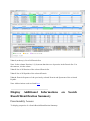
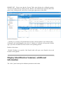
Display Search Result & Identification Summary additional information
Display Spectral Counts
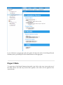
Display XIC
Create and Save a User Window
List of Abbreviations
Frame Toolbars Functionalities
Filter tables
Search tables
Graphics : Scatter Plot / Histogram
Statistical Reports (MSDiag)
Save, import and export
Import Mascot/OMSSA result file
Export data
Algorithm and other operation
Validate a Search Result
Change Typical Protein of a Protein Set
Merge
Data Mixer
Quantitation
Spectral Count
XIC
Refine Protein Sets Abundances
Proline Web
Workflow
Open a session and access to my projects
Register and pair Raw & MzDB files
Create a new project
Import Result Files
Create an Identification Dataset
Validate a Search Result
Create a Quantitation
Delete Datasets
Users management
Create a User
Display
Display peptides and/or PSM in identification result
Display proteins sets in Identification Summary
Display Identification Summary additional information
Save, import and export
Export data
Import Result Files
Algorithm and other operation
Validate a Search Result
Create a Proline project
Command line (ProlineAdmin)
Run the following command line from the ProlineAdmin directory:
Windows :
run_cmd.bat create_project -oid <owner_id> -n <project_name> -desc
<project_description>
Linux :
sh run_cmd.sh create_project -oid <owner_id> -n <project_name> -desc
<project_description>
Note: The project's description is optional.
From graphical tool ProlineAdmin GUI
Click on the “Create a new project” button, then select the project's owner from users list
and set the project's name. You can optionally provide a description for this project.
Note: Since the project's owner must be provided, this functionnality will be disable if
Proline is not set up or if no Proline user is registered yet (see how to set up Proline and
create a Proline user).
Create a Proline user
Command line (ProlineAdmin)
You can create a proline user with the Proline Admin “RunCommand” script. Open a
command line window (Maj + Right Click on Windows) and type the following command:
Windows :
run_cmd.bat create_user -l <user_login> -p <user_password>
Linux :
sh run_cmd.sh create_user -l <user_login> -p <user_password>
From graphical tool ProlineAdmin GUI
You can also use the ProlineAdmin graphical interface: open ProlineAdmin GUI and click
on the “Create user” button. A new window allows you to set the new user's name and
password (with password verification).
Note: This functionality will be disable if Proline is not set up (see how to set up Proline).
From Proline Web Desktop
You can also create users from the Proline Web Desktop administration interface: Create a
User and synchronise it with the Proline Core UDS Database
Proline STUDIO
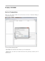
Server Connection
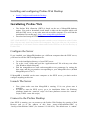
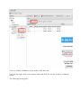
When you start Proline Studio for the first time, the Server Connection Dialog is
automatically displayed.
You must fill the following fields:
- Server Host: this information must asked to your IT Administrator.
- Project User: your name (an account must have been previously created by the IT
Administrator).
- Password: password corresponding to your account.
If you check “Remember Password”, the password will be saved. So, when you will restart the application, Proline Studio will automatically connect to the server and load your
projects without opening the Server Connection Dialog.
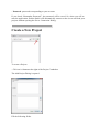
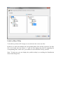
Create a New Project
To create a Project:
- Click on “+“button at the right of the Project Combobox.
The Add Project Dialog is opened.
Fill the following fields:
- Name: name of your project
- Description: description of your project
You can specify other people to share this new project with them.
Then click on OK Button
Creation of a Project can take a few seconds. During its creation, the Project is displayed
grayed with a small glasshour over it.
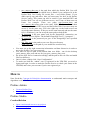
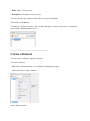
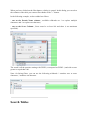
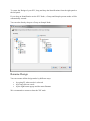
Create a Dataset
You can create a Dataset to group your data.
To create a Dataset:
- right click on Identifications or on a Dataset to display the popup.
- click on the menu “Add > Dataset…”
On the dialog opened:
- fill the name of the Dataset
- choose the type of the Dataset
- optional: click on “Create Multiple Datasets” and select the number of datasets you want
to create
Let's see the result of the creation of 3 datasets named “Replicate”:
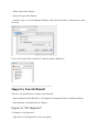
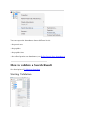
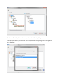
Import a Search Result
There are two possibilities to import Search Results:
- import multiple Search Results in “All Imported” and put them later in different datasets.
- import directly a Search Result in a dataset.
Import in "All Imported"
To import in “All Imported”:
- right click on “All Imported” to show the popup
- click on the menu “Add Search Result…”
In the Import Search Results Dialog:
- select the file(s) you want to import thanks to the file button (the Parser will be
automatically selected according to the type of file selected)
- select the different parameters
- click on OK button
Note 1: You can only browse the files accessible from the server according to the
configuration done by your IT Administrator. Ask him if your files are not reachable.
(Look for Setting up Mount-points paragraph in Installation & Setup page)
Note 2: The “Save Spectrum Matches” option does no longer exist. The Spectrum
matches can be generated on demand when the Search Result is imported.
Note 3: Proline is able to import OMSSA files compressed with BZip2.
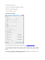
Importing a Search Result can take some time. While the import is not finished, the “All
Imported” is shown grayed with an hour glass and you can follow the imports in the Tasks
Log Window (Menu Window > Tasks Log to show it).
To show all the Search Results imported, double click on “All Imported”, or right click to
popup the contextual menu and select “Display List”
From the All Imported window, you can drag and drop one or multiple Search Result to an
existing dataset.
Import directly in a Dataset
It is possible to import a Search Result directly in an Dataset. In this case, the Search
Result is avaible in “All Imported” too.
To import a Search Result in a Dataset, right click on a dataset and then click on “Add >
Search Result…” menu.
Delete Data
You can delete Search Results, Identification Summaries and Datasets in the data tree. You
can also delete XIC or Spectral Counts in the quantitation tree.
There are two ways to delete data: use the contextual popup or drag and drop data to the
Trash.
Delete Data from the contextual popup
Select the data you want to delete, click the mouse right button to open the contextual
menu and click on delete menu.
The selected data is put in the Trash. So it is possible to restore it while the Trash has not
been emptied.
Delete Data by Drag and Drop
Select the data you want to delete and drag it to the Trash. It is possible to restore data
while the Trash has not been emptied
Empty the Trash
To empty the Trash, you have to Right click on it and select the “Empty Trash” menu.
(In fact, for the moment, Search Results are not completely removed, you can retrieve
them from the “All Imported” window )
Delete a Project
It is not possible to delete a Project by yourself. If you need to do it, ask to your IT
Administrator
Connection Managment
Once user is connected (see Server Connection), it is possible to:
Disconnect
Reconnect with a different login
Change password
Display peptides/PSM or Proteins of a Search
Result
Functionality Access
To display data of a Search Result:
- right click on a Search Result
- click on the menu “Search Result >” and on the sub-menu “PSM” or “Proteins”
Peptides/PSM Window
If you click on PSM sub-menu, you obtain this window:
Upper View: list of all PSM/Peptides.
Middle View: Spectrum, Spectrum Error and Fragmentation Table of the selected PSM. If
no annotation is displayed, you can generate Spectrum Matches by clicking on the
according button
Bottom Window: list of all Proteins containing the currently selected Peptide.
Note: Abbreviations used are listed here
Proteins Window
If you click on Proteins sub-menu, you obtain this window:
Upper View: list of all Proteins
Bottom View: list of all Peptides of the selected Protein.
Note: Abbreviations used are listed here
Display PSM, Peptides or Protein Sets of an
Identification Summary
Functionality Access
To display data of an Identification Summary:
- right click on an Identification Summary
- click on the menu “Identification Summary >” and on the sub-menu “PSM”, “Peptides”
or “Protein Sets”
PSM Window
If you click on PSM sub-menu, you obtain this window:
Note : Abbreviations used are listed here
Peptides Window
If you click on Peptides sub-menu, you obtain this window:
Upper View: list of all Peptides
Middle View: list of all Protein Sets containing the selected peptide.
Bottom Left View: list of all Proteins of the selected Protein Set
Bottom Right View: list of all Peptides of the selected Protein
Note: Abbreviations used are listed here
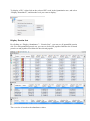
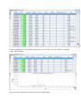
Protein Sets Window
If you click on Protein Sets sub-menu, you obtain this window:
View 1 (at the top): list of all Protein Sets
Note: In the column Proteins, 8 (2,6) means that there are 8 proteins in the Protein Set. 2 in
the sameset, 6 in the subset.
View 2: list of all Proteins of the selected Protein Set.
View 3: list of all Peptides of the selected Protein
View 4: Protein Sequence of the previously selected Protein and Spectrum of the selected
Peptide.
Note: Abbreviations used are listed here
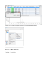
Display Additional Informations
Result/Identification Summary
Functionality Access
To display properties of a Search Result/Identification Summary:
on
Search
- right click on a Search Result/Identification Summary
- click on the menu “Properties”
Note: it is possible to select multiple Search Results/Identification Summaries to compare
the values.
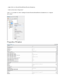
Properties Window
Display a Spectral Count
You can display a generated Spectral Count by using the right mouse popup.
To have more details about the results, see spectral count result
Display a XIC
To display a XIC, right click on the selected XIC node in the Quantitation tree, and select
“Display Abundances”, and then the level you want to display:
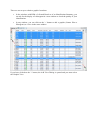
Display Protein Sets
By clicking on “Display Abundances” / “Protein Sets”, you can see all quantified protein
sets. For each quantified protein set, you can see below all peptides linked to the selected
protein set and peptides Ions linked to the selected peptide
The overview is based on the abundances values.
For each quantitation channel, are displayed:
- The raw abundance
- The peptide match count (by default)
- The abundance (by default)
- The selection level
By clicking on the “Column Display Button”
to display.
, you can choose the information you want
To display the identification protein set view, click right on the selected protein Set and
select “Display Identification Protein Sets” menu in the popup.
Display peptides
By clicking on “Display Abundances “/ “Peptides”, you can see:
- identified and quantified Peptides
- non identified but quantified peptides
- identified but not quantified peptides (linked to a quantified protein)
Display Peptides Ions
By clicking on “Display Abundances” / “Peptides Ions”, you can see:
- all identified and quantified Peptides Ions
- non identified but quantified peptides Ions
Create a User Window
You can lay out your own user window with the desired views.
You can do it from an already displayed window or by using the right click mouse popup
on a dataset like in the following example (Use menu “Search Result>New User
Window…” or “Identification Summary>New User Window…”)
In the example, the user has clicked on “Identification Summary>New User Window…”
and selects the Peptides View as the first view of his window.
You can add other views by using the '+' button.
In this example, the user has added a Spectrum View and he saves his window by clicking
on the “Disk” Button.
The user selects 'Peptides Spectrum' as his user window name
Now, the user can use his new 'Peptides Spectrum' on a different Identification Summary.
List of Abbreviations
Calc. Mass : Calculated Mass
Delta MoZ : Delta Mass to Charge Ratio
Ion Parent Int. : Ion Parent Intensity
Exp. MoZ : Experimental Mass to Charge Ratio
Missed Cl. : Missed Clivage
Next AA : Next Amino-Acid
Prev. AA : Previous Amino-Acid
Protein S. Matches : Protein Set Matches
PSM : Peptide Spectrum Match
PTM : Post Translational Modification
RT : Retention Time
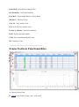
Frame Toolbars Functionnalities
A : Display Decoy Data.
B : Search in the Table. (using * and ? wild cards)
C : Filter data displayed in the Table
D : Export data displayed in the Table
E : Send to Data Mixer to compare data from different views
F : Create a Graphic : histogram or scatter plot
G : Right click on the marker bar to display Line Numbers or add Annotations/Bookmarks
H : Expands the frame to its maximum (other frames are hidden).
I : Gather the frame with the previous one as a tab.
J : Split the last tab as a frame underneath
K : Remove the last Tab or Frame
L : Open a dialog to let the user add a View (as a Frame, a Tab or a splitted Frame)
M : Save the window as a user window, to display the same window with different data
later
N : Export view as an image
O : Generate Spectrum Matches
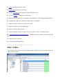
Filter Tables
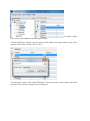
You can filter data displayed in the different tables thanks to the filter button at the top
right corner of a table.
When you have clicked on the filter button, a dialog is opened. In this dialog you can select
the columns of the table you want to filter thanks to the “+” button.
In the following example, we have added two filters:
- one on the Protein Name column ( available wildcards are * to replace multiple
characters and ? to replace one character)
- one on the Score Column ( Score must be at least 100 and there is no maximum
specified).
The result is all the proteins starting with GLPK ( correspond to GLPK* ) and with a score
greater or equal than 100.
Note: for String filters, you can use the following wildcards: * matches zero or more
characters, ? matches one character.
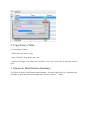
Search Tables
In some tables, a Search Functionality is available thanks to the search button at the top
right corner.
When you have clicked on the search button, a floating panel is opened. In this panel you
can fill in the searched expression. Two wild cards are available:
'*' : can replace all characters
'?' : can replace one character
In the following example, the user search for a ProteinSet whose name starts with
“DNAK”.
You can do an incremental search by clicking again on the search button of the floating
panel.
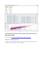
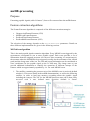
Graphics
Create a Graphic
There are two ways to obtain a graphic from data:
In the windows with PSM of a Search Result or of an Identification Summary, you
can ask for the display of a histogram in a new window to check the quality of your
identification.
In any window, you can click on the '+' button to add a graphic (Scatter Plot or
Histogram) as a view in the same window
If you have clicked on the '+' button, the Add View Dialog is opened and you must select
the Graphic View
Graphic options
A: Display/Remove Grid toggle button
B: Modify colour of the graphic
C: Lock/Unlock incoming data. If it is unlocked, the graphic is updated when the user
apply a new filter to the previous view (for instance Peptide Score >= 50 ) If it is locked,
changing filtering on the previous view does not modify the graphic.
D: Select Data in the graphic according to data selected in table in the previous view.
E: Select data in the table of the previous view according to data selected in the graphic.
F: Export graphic to image
G: Select the graphic type : Scatter Plot / Histogram
H/I: Select data used for X / Y axis.
It is possible to select linear or log axis by right clicking on an axis.
Zooming / Selection
Zoom in: Press the right mouse button and drag to the right bottom direction. A red box is
displayed. Release the mouse button when you have selected the area to zoom in.
Zoom out: Press the right mouse button and drag to the left top direction. When you
release the mouse button, the zooming is reset to view all.
Select: Press the left mouse button and drag the mouse to surround the data you want to
select. When you release the button, the selection is done. Or left click on the data you
want to select. It is possible to use Ctrl key to add to the previous selection.
Unselect: Left click on a empty area to clear the selection.
Statistical Reports (MSDiag)
In order to launch MSDiag Reports (statistical reports), simply select a node on the tree
and choose 'Compute statistical reports' and wait for the results to appear. This applies to a
search result only. (Not possible for a dataset)
Choose the menu option:
You then configure some settings before launching the process.
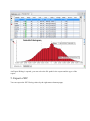
Your report will appear in a matter of seconds (depending of the amount of data to be
processed).
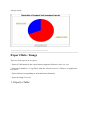
You have other types of display that are possible:
Histograms:
And pie charts:
Export Data / Image
There are four ways to do an export :
- Export a Table thanks to the export button (supported format are xlsx, xls, csv)
- Export data thanks to a Copy/Paste from the selected rows of a Table to an application
like Excel.
- Export all data corresponding to an Identification Summary
- Export an image of a view
1. Export a Table
To export a table,
click on the Export Button at the left top of a table.
An Export Dialog is opened, you can select the file path for the export and the type of the
export ( Excel (.xlsx); Excel (.xls) or CSV. )
To perform the export, click on the OK Button. The task can take a few seconds if the table
has a lot of rows and so a progress bar is displayed.
2. Copy/Paste a Table
To copy/Paste a Table :
- Select rows you want to copy
- Press Ctrl and C keys in the same time
- Open for example excel and press Ctrl and V keys in the same time to paste the copied
rows.
3. Export an Identification Summary
To Export all data of an Identification Summary, you must right click on a Identification
Summary to open the contextual popup and select the “Export…” Menu.
An Export Dialog is opened, you can select the file path for the export and the type of the
export ( only Excel (.xlsx) is available for the moment).
You can select the “Export All PSMs” option to add a sheet with all PSMs for each Protein
Set.
Description of exported file is available here.
4. Export an Image
To export a graphics, click on the Export Image Button at the left top of the image.
An Export Dialog is opened, you can select the file path for the export and the type of the
export
5. Export a XIC
You can export the XIC Desing values by the right mouse button popup.
You can export the abundances data at different levels:
- the protein sets
- the peptides
- the peptides ions
- the refined protein sets abundances (see Refine Protein Sets Abundances)
How to validate a Search Result
See description of Validation Algorithm.
Starting Validation
To validate a Search Result:
- Select one or multiple Search Results to validate
- Right Click to display the popup
- Click on “Validate…” menu
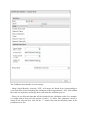
Validation Dialog
In the Validation Dialog, fill the different Parameters (see Validation description) :
- you can add multiple PSM Prefilter Parameters ( Rank, Length, Score, e-Value, Identity
p-Value, Homology p-Value) by selecting them in the combobox and clicking on Add
Button '+'
- you can ensure a FDR on PSM which will reached according to the variable selected (
Score, e-Value, Identity p-Value, Homology p-Value,… )
- you can add a Protein Set Prefilter on Specific Peptides.
- you can ensure a FDR on protein Sets.
- you can set the choice for the Typical Protein of a Protein Set by using a match string
with wildcards ( * or ? ) on Protein Accession or Protein Description. (See Chang Typical
Protein of Protein Sets)
Note: FDR can be used only for Search Results with Decoy Data.
Validation Processing
Validating a Search Result can take some time. While it is not finished, the Search Results
are shown greyed with an hour glass over them. The tasks are displayed as running in the
“Tasks Log Dialog”.
Validation Done
When the validation is finished, the icon becomes orange and blue. Orange part
corresponds to the Identification Summary. Blue is for the Search Result part.
Change Typical Protein of Protein Sets
The protein sets windows are not updates after a Change Typical Protein ! You should
close and reopen the window
Open the Dialog
To change the Typical Protein of the Protein Sets of a Identification Summary:
- Select one or multiple Identification Summaries
- Right Click to display the popup
- Click on “Change Typical Protein…” menu
Dialog Parameters
You can set the choice for the Typical Protein of Protein Sets by using a match string with
wildcards ( * or ? ) on Protein Accession or Protein Description.
Three rules could be specified and they will be applied in priority order. In a Protein Set, if
no proteins satisfy the first rule, the second one will ne tested and so on.
Processing
The modification of Typical Proteins can take some time. During the processing,
Identification Summaries are displayed grayed with an hourglass and the tasks are
displayed in the Tasks Log Window
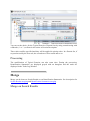
Merge
Merge can be done on Search Results or on Identification Summaries. See description for
Search Results merging and Identification Summaries merging
Merge on Search Results
To merge a dataset with multiple Search Results:
- Select the parent dataset
- Right Click to display the popup
- Click on “Merge” menu
When the merge is finished, the dataset is displayed with an M in the blue part of the icon,
indicating that the Merge has been done at a Search Result level.
Merge on Identification Summaries
If you merge a dataset containing Identifications Summaries. The merge is done on a
Identification Summary level. Therefore the dataset is displayed with an M in the orange
part of the icon.
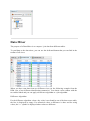
Data Mixer
The purpose of a Data Mixer is to compare / join data from different tables.
To send data to the data mixer, you can use the dedicated button that you can find in the
toolbar of all views.
When you have sent data from two different views (in the following example from the
PSM view of two different identification summaries). You obtain a new window with the
two tables linked and you can apply a difference algorithm or a join algorithm.
Difference Algorithm
For the difference algorithm: when a key value is not found in one of the data source table,
the line is displayed as empty. For numerical values a difference is done and for string
values, the '<>' symbol is displayed when values are different.
Join Algorithm
In the following example, we have used the join algorithm and added a graphics thanks to
the '+' to compare the scores of the PSM from two identification summaries.
Spectral Count
See description of Compare Identification Summaries with Spectral Count .
Generate a Spectral Count
To obtain a spectral count, right click on a Dataset with merged Identification Summaries
and select the “Compare with SC” menu in the popup.
In the Spectral Count window, fill the name and description of your Spectral Count and
press Next.
Then select the Identification Summaries on which you want to perform the Spectral Count
and press OK.
A Spectral Count window is opened with a label indicating that the calculation is being
done, and the Spectral Count is added to the Quantitation’s Panel.
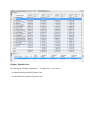
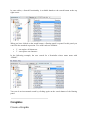
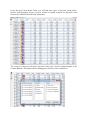
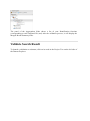
Spectral Count Result
In the Spectral Count Result Table, you will find three types of Spectral Count: Basic,
Specific and Weighted, and an overview column to rapidly compare the Spectral Count
between the different Identification Summaries.
The overview is based on the Basic Spectral Count, but it can be changed thanks to the
Column Buttons. This button allows changing the visibility of the columns too.
Comparing Spectral Counts
If you sort the column Overview by clicking on its header, you will be able to easily find
the proteins with Spectral Counts different from one Identification Summary to another.
Display a Spectral Count
You can later display again an already generated Spectral Count, see Display a Spectral
Count
XIC Quantitation
For description on LCMS Quantitation you can first read the principles in this page:
Quantitation : principles
Generate a XIC
To generate a XIC, right click on the Quantitations Node and select the “Extract
Abundances” menu in the popup.
Create Design
To create the Design of your XIC, drag and drop the identifications from the right panel to
the left panel.
If you drop an identification on the XIC Node, a Group and Sample parents nodes will be
automatically created.
You can also directly drop on a Group or Sample Node.
Rename Design
You can rename all the design nodes by different ways:
by typing F2 when a node is selected
by a long click on a node
by the right button popup and the menu Rename
We recommend to rename at least the XIC node.
Link to Raw Files
To be able to perform a XIC design, we need to know the source raw files.
Proline try to find in the database the corresponding Raw Files already registered. If a Raw
file is not found, the icon shows a '!' and you can display the error by expanding the
corresponding node. In this case, you will have to select the Raw File by yourself.
Note: To help you, you can display the peaklist tooltip by overriding the Identifcation
Node in the Design Tree.
To select a Raw File, click on the error, and use the following dialog.
You can select directly a file on the disk or a potential corresponding Raw File registered
in the database.
XIC Parameters
When the XIC Design is finished, click on the next button and select the parameters. See
Label-free LC-MS quantitation configuration to have more details about the different
parameters.
Note: all the parameters are already set with default values.
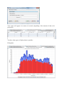
XIC Results
When the XIC Design has been generated, it is added in the Quantitation Tree. You can
display its properties, especially the configuration used, by the right mouse button popup:
You can delete a XIC Design, see how to Delete Data
You can rename a XIC Design, by clicking on “Rename…” in the popup menu.
You can export the XIC results, see how to Export a XIC
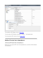
Refine Protein Sets Abundances
Advanced Protein Sets abundances
Right click on the selected XIC node in the Quantitation tree, and select “Refine Proteins
Sets Abundances…”
Configuration
In the dialog, you can:
- specify peptides to consider for quantitation
- configure parameters used for peptides quantitation
- configure parameters used for proteins quantitation
For more details, see Post-processing of LC-MS quantitative results
Advanced XIC results
You can see the results by displaying the XIC (Display a XIC) or export them (Export a
XIC)
Proline WEB
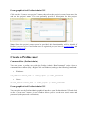
Server Connection
Prerequisite: You must have an account to login to the server. Ask your administrator to
create one if you don't have any. After the installation, the default account is “admin”
with password “admin”
- Open your Google Chrome web browser and connect to the address of the server (ask
your administrator)
- Enter your username and password and click “OK”.
- To create a project, please follow the instructions detailed on this page.
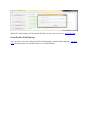
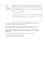
Register Raw & MzDB Files
In order to create and run Quantitation analyses, you must register your RAW files and
corresponding MzDB files into Proline databses to do so, click on the “Settings” button in
the top bar of the Dataset Explorer application, and go to the “Raw File Registerer” tab.
In the left grid, use the “Add Raw Files to Selection” button in order to select Raw
Files
In the right grid, use the “Add MzDB Files to Selection” button in order to select
MzDB Files
You can then make automatic pairs, based on file names, by clicking on the “Make
Couples from RAW Files” button. This will automatically add matching files into
the “Raw & MzDB Couples” grid.
If you want to pair files whose names differ, you can proceed as follows:
Select a file, either Raw or MzDB, in its grid,
Click on the “Put in Couple” button,
Select it in the “Raw & MzDB Couples” grid,
Select the corresponding file of the other format (RAW or MzDB) in its grid,
Click on its “Put in Couple” button.
After this, you must choose an Instrument Name and select the owner of the file in the
users list.
Finally, click on “Register”. Note that this operation will fail if one of your raw file has
already been registered.
Close the Settings Window.
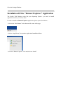
Installation Of the "Dataset Explorer" Application
The Proline Web Desktop works like your Operating System : you need to install
applications before you can use them.
In order to install the Dataset Explorer application, please proceed as follows :
- click on the “Start Button” in the bottom-left corner of the page,
- click on “App Library” to open the Application Installation Menu
- select the “Dataset Explorer” Line and click on “Install”
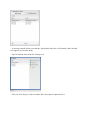
- A message should inform you that the Application has been well installed, and it should
now appear in your start menu
- Open it from the start menu by clicking on it
- Click on “New Project” and set a name and a description (optional) for it
- Once your project is created, you can see it in the tree on the left of the screen. Click on it
to make its options panel appear.
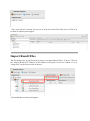
Import Result Files
The first thing to do in your brand new project is to import Result Files. To do so, Click on
the “Import Result File” Button, in the toolbar of the project overview window or via a
“right-click” on the Project node of the tree
You should then see this panel appear:
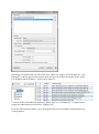
It allows you to select Result Files and set up following parameters for the import process:
Parameters
o Software Engine : the software which generated your interrogation file
o Instrument : mass-spectrometer used for sample analysis
o Peaklist Software : the software used for the peaklist creation
Decoy Parameters
o Decoy Strategy : TODO
o Protein Match Decoy Rule : TODO
Parser Parameters: according to your Software Engine, this will display some extraparameters.
o Mascot :
Ion Score Cutoff : TODO
Subset Threshold : TODO
Mascot Server URL : TODO
o Omssa :
User mod file : TODO
PTM Composition File : TODO
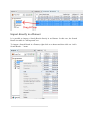
Check Files before Import: let this checked to ensure that your files contain no
errors. The server will perform a check operation before launching the import.
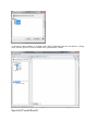
In order to add files to your import selection, click on “Select Result File” to open the File
Browser that will let you choose one or many result files to import:
The left side let you browse the directories, and when you click on one of them, its content
is shown on the main panel. Choose one or multiple files then click “Ok”.
Back to the “Import Result File” window, you should now see your selection appear in the
grid. Choose the instrument and the peaklist software corresponding to your files, and then
select a “Decoy Strategy”. You can now click on “Start Import” to launch the check and
the import tasks.
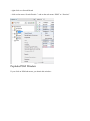
The server will check your files first, then the import itself will be launched automatically.
You can follow the current state of your tasks by clicking on the small cake in the bottom
right corner of the desktop screen. It opens a small grid where you can see all your tasks.
When a task is done, you are notified by a small message in the top of the screen, and you
can see its status in the tasks window:
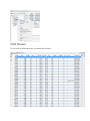
All the Result Files you have imported are listed in the “Search Results” panel you can
access by double-clicking the “Search Results” node in your project's tree.
------------
Create a new Dataset
Once your Result Files have been imported, you can use them to create a new
Identification Dataset. Double-Click on the “Identification Trees” element in the tree, on
the left side of the window. The grid which just appeared is meant to list all your datasets.
For now, click on the “New Dataset” button from the bar, or by right-clicking on the
“Identification Trees” node.
You should now see a window asking to choose a source of data for your new Dataset.
Choosing “Result Set” allows you to build a new dataset from both Result Files you
have imported and existing identification datasets, whether they have been
validated or not.
Choosing “Result Summary” will let you build a new dataset from one or more
existing validated identification dataset. Il will duplicate them into a new Dataset
without their validation data.
For now, assuming you are creating your first identification dataset, you should choose the
“Result Set” option. On the two-tabbed panel, go to the “Result Sets” tabs in order to see
the list of the files you have imported.
To add one or many files to your selection, select them in the grid (you can use the Ctrl and
the Shift keys to make a multiple selection), then click on “Add to Selection” on the
bottom of the window. You can also double click on one file to quickly add it to the
selection.
To remove any file from the selection, just select them and click on “Remove selected
Items”. Type a name for your dataset then click on “Create”. The creation of your
identification dataset happens as follows:
An “Aggreagation” Dataset Node is created. It takes the name that you provided
during the creation.
One “Identification” Dataset Node is created for each one of the Result Files you
have selected. They take the name of the Result File.
Once your Identification Dataset has been created, you can see it on the tree, in the left side
of the window.
The panel of the Aggregation Node shows a list of your Identification fractions
(corresponding to each imported file) and, after the validation process, it will display the
Merged Result Summary infos.
Validate Search Result
To launch a validation on a dataset, click on its node in the Project Tree on the left side of
the Dataset Explorer.
Click on “Launch Validation” in the toolbar of the Infos tab.
You can also right click on the dataset node and click on use the “Launch Validation”
button.
The following form appears:
The Validation form handles several settings:
- Merge Search Results: choosing “YES” will merge the Result Sets (corresponding to
your result files) before launching the validation of the merged dataset. “NO” will validate
the result sets separately and merge their result after the validation process.
- Filters: let you filter the data that will be included in the validation results. For example,
you might want to keep only the peptide of rank 1. To add a filter parameter, choose a
setting in the selection box, click on the “+” button, then edit the threshold value of the
parameter on its line.
- Validation Thresholds let you define the False Discovery Rate of your peptides and
proteins. You must define from which parameter the Peptide FDR should be estimated:
When ready, click on “Validate” to launch the validation task. You can see it in the tasks
panel.
Create a Quantitation
Double-click on the “Quantitations” node of your project tree to show you Quantitations
table panel. It's empty if you haven't created any quantitation in this project yet. Click on
the “New Quantitation” button to open the Quantitation Creation Panel.
Note that you can also open it by right-clicking on the Quantitation node or on the Project
node itself.
Title, Type and Method
The first tab of the Quantitation creation panel let you define a name, a description
(optional), choose a type and a method.
Once you've made your choices, click on “Next”.
Experimental Design
The Experimental design tab is where you define your Groups and Samples. By default,
two groups are created and each one contains a sample.
You can create new groups by clicking on the “Add Group” button in the top bar of the
tab. In each group, you can manage your sample by using the buttons in the left grid.
To add a Search Result to one of the samples of the group, select it in the left grid, and
drag and drop a validated result set from your project's tree to the “Sample
Analyses” grid
Once you have prepared all your group and samples, click on the “Next” button.
Abundance Extraction parameters
This tab let you set up you abundance extraction parameters.
Ratios
The purpose of this tab is to define the ratios between the groups your quantitation will rely
on
Launch the Analysis
When you're done, just press the “Launch Quantitation” button. You will be noticed when
the task is finished
Delete Datasets
You can delete an Identification dataset by clicking on it on the Dataset Explorer left side
panel, and then click on the “Move to Trash” button in the toolbar of the “Infos” tab.
You can also right click on the dataset you want to delete, and click on the “Move to
Trash” button.
All deleted datasets are visible in the “Trash” node in the project tree.
Create a User
You must be logged in as an administrator.
Click the “Start” button, go to “Administration”. On the first tab, “User Administration”,
you can create a new user by setting up its name, its password, and define whether or not
the user will have the “administration” permissions (including applications, users and
service management).
Submit the form to create the user. You can manage existing users from the “users” tab.
Please note that the Proline Web Desktop has its own database and its own users
collection. However, if you configured the Proline Service running inside the Proline Web
Desktop, it will synchronise the Proline Web Desktop and the Proline Core users each time
a user logs in the Proline Web Desktop:
the users you create in the Proline Web Desktop Administration panel will be
automatically added to the Proline Core database (User Data Set database) when
they sign in on the Proline Web Desktop.
the Users registered in the Proline Core Database (UDS) will be automatically
registered in the Proline Web Desktop database when you log in as administrator in
the Proline Web Desktop, if they were missing.
Peptides Table
The “Peptides” tab of a validated Identification Dataset (or Merged Dataset) allows you to
browse the peptides of the related Result Summary.
Each table of the Result Summary data viewer provides a set of Filters for Numerical, Text
and Boolean data, placed on the left of the grid.
Peptide Click Actions:
- Clicking on a Peptide will automatically display the peptides matches related to the
selected peptide on the Peptide Matches table, and the Protein Matches table will display
the protein matches related to the selected peptide.
Double Click actions:
- If you double click on a peptide match, an MS Queries viewer tab focused on the
corresponding ms query (a filter will automatically applied) will be opened.
- If you double click on a protein match, a Proteins viewer tab focused on the
corresponding protein will be opened.
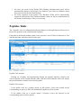
MS Queries Table
The MS Queries table displays the MS Queries of the Result Summary and offers the same
filters options as the others tables.
MS Query Click:
- Clicking on an MS Query will automatically load the corresponding Peptide Matches in
the “MS Query Peptides Matches” table
Double Click Actions:
- Double clicking on a Peptide Match item will open a Peptides viewer tab focused on the
corresponding peptide.
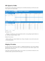
Display Proteins
In order to browse the protein set data of a validated identification, click on the validated
identification node in the project tree, on the left side panel of the dataset explorer, and
then open the “Proteins” tab.
Each table of the Result Summary data viewer provides a set of Filters for Numerical, Text
and Boolean data, placed on the left of the grid.
IMPORTANT : Please note that the Protein Table only displays the validated proteins.
You can reset this filter by clicking on the “Remove All” button of the proteins table filter
panel, or by clicking on the circle arrow in the upper right corner of the table.
Protein click action:
- Clicking on a protein will automatically load the related peptides in the bottom table. Clicking on the small Magnifier near the AC Number of a protein will open the UniProt
app (if you have installed id) focused on the corresponding protein.
Double click actions:
- Double Clicking on a peptide of the Peptide table will open a new Peptide viewer tab
focused on this peptide.
Display Identification Summary additional
information
The “Infos” panel sums up the validation parameters and results.
If you clicked on an Aggregate node, this panel will show the infos of the Merged Result
Summary and a grid listing all of the identifications of this aggregate.
Export Data
To export any of the Result Summary data table, just click on the save icon on the top of
the table. Please note that any current filter applied to the table will be applied to the
exported data.
Raw file conversion to mzDB
raw2mzDB installation
1. get the zip archive
2. installation of MSFileReader from Thermo ( here, will install all necessary c++
redistribuables)
3. Ensure your regional settings parameters are '.' for the decimal symbol and ',' for the
list separator
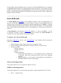
Use case procedure
Open a command line window in the directory containing raw2mzdb.exe
Type:
raw2mzdb.exe
-i
<rawfilename>
-o
<outputfilename>
By defaut, the raw file will be converted in the “fitted” mode for the MS1 (MS2 is often in
centroid mode and can not be converted in fitted mode). If the MS2 (or superior) are
acquired in high resolution (i.e in profile mode), you could specify that you want to
convert several MSs in the required mode: raw2mzdb.exe -i <rawfilename> -o
<outputfilename> -f 1-2 will try to convert MS1 to MS2 in fitted mode.
There are two other available conversion modes:
1. “profile”, the command line is then: raw2mzdb.exe -i <rawfilename> -o
<outputfilename> -p 1 (means you want profile mode for MS1, others MS will be
stored as they were stored in the raw file)
2. “centroid” : raw2mzdb.exe -i <rawfilename> -o <outputfilename> -c 1 (means
you want centroid mode for MS1, others MS will be stored as they were stored in
the raw file)
CONCEPTS
Proline Concepts & Principles
Dataset types:
o Result File
o Search Results
o Decoy Searches
o Identification Summary
Data Processings:
o Protein Inference
o Protein and Proteins Sets scoring
o FDR Estimation
o Validation Algorithm
o Merge multiple Search Results
o Merge multiple Identification Summaries
o Compare with Spectral Count
o Quantitation (Principle)
LC-MS quantification
LC-MS quantification workflows
mzDB-processing
Label-free LC-MS quantitation workflow
o Quantitation (Configuration)
Label-free LC-MS quantitation configuration
Post-processing of LC-MS quantitative results
Data Import/Export:
o Identification Summary Export
Result File
A Result File is the file created by a search engine when a new search is submitted.
OMSSA (.omx files) and Mascot (.dat files) search engines are currently supported by
Proline. A first step when using Proline is to import Result Files through Proline Studio or
Proline Web.
Search engines provide different types of searches for MS and MS/MS data. It is important
to highlight that the Result File content depends on the search type. Thus, Mascot searches
must be currently performed using MS/MS ions search in order to be properly imported by
Proline. Peptide Mass Fingerprint and MS/MS error tolerant searches will be supported in
further versions of Proline.
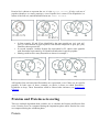
Search Result
A Search Result (aka ResultSet in the database schema) is the raw interpretation of a
given set of MS/MS spectra given by a search engine or a de novo interpretation process. It
contains one or many peptides matching the submitted MS/MS spectra (PSM, i.e. Peptide
Spectrum Match), and the protein sequences these peptides belong to. The Search Result
also contains additional information such as search parameters, used protein sequence databank, etc.
A Search Result is created when a Result File (Mascot .dat file or an OMSSA .omx) file
is imported in Proline. In the case of a target-decoy search, two Search Results are
created: one for the target PSMs, one for decoy PSMs.
Content of a Search Result
Importing a Result File creates a new Search Result in the database which contains the
following information:
Search Settings: software name and version, parameters values
Peak-List and Spectrum information: file name, MS level, precursor m/z, …
Search result data:
o Protein sequences
o Peptide sequences
o Spectra
o 2 kinds of Matches
Peptide Spectrum Matches, i.e. the matching between a peptide and
a spectrum, with some related data such as the score, fragment
matches…
Protein Matches, i.e. the proteins in the databank corresponding to
the PSMs identified by the search engine
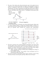
Mascot result importation
The peptide matches score correspond to Mascot ion score
OMSSA result importation
The peptide matches score correspond to the negative common logarithm of the E-value:
Score = -log10(E-value)
Decoy Searches
Proline handles decoy searches performed from two different strategies:
Concatenated searches:
o A protein databank is created by concatenating target protein sequence to
decoy protein sequence. Deoy could be created using reverse or random
strategie. From Mascot or OMSSA point of view, a unique search is done
using that databank.
Separated searches:
o Two searches are done using the same peaklist, one on a target protein
databank and one on a decoy protein databank. These searches are then
combinated to retrieve usefull information such as FDR … Mascot allows
user to check a decoy option and will automalically create a decoy
databank.
Decoy and Target Search Result
Concatenated searches:
o When importing search result from a decoy concatenated databank, decoy
data are extracted from the Result File and stored in Proline databases as an
independant/unique Search Result as well as target Search result data. These
both searches are linked to each other.
Separated searches
o The two performed searches are stored in Proline databases and are linked
together.
See Search Result to view which information is saved
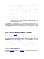
Identification Summary
An Identification Summary (aka ResultSummary) is a set of identified proteins inferred
from a subset of the PSM contained in the *Search Result*. The subset of PSM taken into
account are the PSM that have been validated a filtering process (example: PSM fulfilling
some specified criteria such as score greater than a threshold value).
Content of an Identification Summary
Peptide Set
Protein Set
Typical Protein
sameset
strict subset
subsumable peptide set
Search Results
content
and
Identification
Summary
Search Result
Importing a Result File creates a new Search Result in the database which contains the
following informations:
Search Settings : software name and version, parameters values
Peak List and Spectrum information: file name, ms-level, precursor moz, …
Search result data:
o Proteins
o Peptide
o Spectrum
o 2 type of Matches
a Peptide Match is a match between a peptide and a spectrum, with
score, fragment matches …
a Protein Matches is a match between a peptide and a protein
Mascot result importation
The peptide matches score correspond to Mascot ion score
OMSSA result importation
The peptide matches score correspond to the negative common logarithm of the Evalue:
o Score = -log10(E-value)
Identification Summary
Protein Set :
Peptide Set :
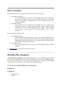
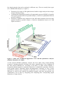
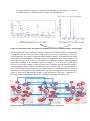
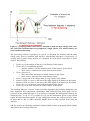
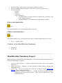
Protein Inference
All peptides identifying a protein are grouped in a Peptides Set. A same Peptides Set can
identify many proteins, represented by one Proteins Set. In this case, one protein of this
Protein Set is chosen to represent the set, it is the Typical Protein. If only a sub set of
peptides identify a (or some) protein(s), a new Peptide Set is created. This PeptideSet is a
subset of the first one, and identified Proteins are Subset Proteins.
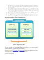
In first example, P2 and P5 are identified by the same peptide set {pe1, pe4, pe5,
pe8}. P2 was choosen as typical protein. One SubSet composed of {pe4, pe5, pe8}
identifies subset protein P4.
In second example, Another Protein Set represented by P3, shares some peptides
with ProteinSet represented by P2. Both ProteinSets have specific peptides.
Sharing could involve many ProteinSet as shown in example 3.
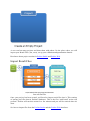
All Peptides Sets and associated ProteinSets are represented, even if there are no specific
peptides. In both cases of above example, no choice is done on which ProteinSet /
PeptideSet to keep. These ProteinSets could be filtered after inference (see Protein sets
filtering).
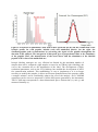
Proteins and Proteins sets scoring
There are multiple algorithms than could be use to calculate the Proteins and Protein Sets
score. Proteins score are computed during the importation phase while Protein Sets score
are comptued during the validation phase.
Protein
Each individual protein match is scored according to all peptide matches associated with
this protein, independently of any validation of these peptide matches. Currently, when
importing Mascot result file : the Mascot standard scoring is used (sum of peptide
matches scores)
importing OMSSA result file :
Protein Set
Each individual protein set is scored according to the validated peptide matches belonging
to this protein set (see inference).
Scoring schemes
Mascot Standard Scoring
The score associated to each identified protein (or protein set) is the sum of the score of all
peptide matches identifying this protein (or protein set). In case of duplicate peptide
matches (peptide matched by multiple queries) only the match with the best score is
considered.
Mascot MudPIT Scoring
This scoring scheme is also based on the sum of all non-duplicate peptide matches score.
However the score for each peptide match is not its absolute value, but the amount that it is
above the threshold: the score offset. Therefore, peptide matches with a score below the
threshold do not contribute to the protein score. Finally, the average of the thresholds used
is added to the score. For each peptide match, the “threshold” is the homology threshold if
it exists, otherwise it is the identity threshold. The algorithm below illustrates the MudPIT
score computation procedure:
Protein
score
=
0
For
each
peptide
match
{
If there is a homology threshold and ions score > homology threshold {
Protein
score
+=
peptide
score
homology
threshold
}
else
if
ions
score
>
identity
threshold
{
Protein
score
+=
peptide
score
identity
threshold
}
}
Protein score += 1 * average of all the subtracted thresholds
if there are no significant peptide matches, the protein score will be 0.
homology and identity threshold values depend on a given p-value. By default
Mascot and Proline compute these thresholds with a p-value of 5%.
In the case of separated target-decoy searches we obtain two values for each
threshold : one for the target search and another one for the decoy search. In order
to obtain a single value we apply the following procedure:
o the homology threshold is the decoy value if it exists else the target value
o the identity threshold is the mean of target and decoy values.
The benefit of the MudPIT score over the standard score is that it removes many of the
junk protein sets, which have a high standard score but no high scoring peptide matches.
Indeed, protein sets with a large number of weak peptide matches do not have a good
MudPIT score.
Mascot Modified MudPIT Scoring
This scoring scheme, introduced by Proline, is a modified version of the Mascot MudPIT
one. The difference with the latter is that it does not take into account the average of the
substracted thresholds. This leads to the following scoring procedure:
Protein
score
=
0
For
each
peptide
match
{
If there is a homology threshold and ions score > homology threshold {
Protein
score
+=
peptide
score
homology
threshold
}
else
if
ions
score
>
identity
threshold
{
Protein
score
+=
peptide
score
identity
threshold
}
}
This score has the same benefits than the MudPIT one. The main difference is that the
minimum value of this modified version will be always close to zero while the genuine
MudPIT score defines a minimum value which is not constant between the datasets and the
proteins (i.e. the average of all the subtracted thresholds).
FDR Estimation
There are several ways to calculate FDR depending on the database search type. In Proline
the FDR is calculated at peptide and protein levels using the following rules:
if the Search has been done on a concatenated Target/Decoy bank, FDR = 2 * nbr
DecoyPSM / (nbr TargetPSM + bnr DecoyPSM ). Note: when computing PSM
FDR, peptide sequences matching a Target Protein and a Decoy Protein is taken
into account in both cases.
if the Search has been done on a separated Target/Decoy bank, FDR = nbr
DecoyPSM / nbr TargetPSM.
Validation Algorithm
Once a result file have been imported and a search result created, the validation is
performed in 4 mains steps :
1.
2.
3.
4.
Peptide Matches filtering and Validation
Protein Inference (peptides and proteins grouping)
Protein and Proteins Sets scoring
Protein Sets Filtering and Validation
Finally, the Identification Result issued from these steps is stored in the identification
database. Different validation of a Search Result can be performed and a new Identification
Summary of this Search Result is created for each validation.
Merger Search Results
Merging several Search Results consist in creating a parent Search Result which will
contain all merged PSMs issued from child Search Result. For each identified peptide
(in at least one child), a single merged PSM will be created and filled with the best child
attributes (score, missed cleavage, etc). The best child PSM is the PSM with the higher
score.
Once a parent Search Result is created, the same validation operation as the one
accessible for new imported Search Result could be done. In this case, the generated
Identification result is not linked to Identification Result associated to child
Search Result.
An other merge algorithm could be used : see Merge Identification Results
Merge Identification Results
This merge operation consists in creating a parent Identification Result from few
child ones. A Search Result corresponding to this parent Identification Result will
be generated.
Concretely, the first step of this merge operation consist in creating merged PSMs for all
peptides identified and validated in at least one child Identification Result. Protein
Inference will then be applied to create the parent Identification Result.
Compare Identification Summaries with Spectral
Count
Definition
The peptide spectral count consist in counting the number of spectra which
matches the current peptide. Thus, it's equal to the number of pepitde spectrum
matches (PSM).
Protein basic spectral count (BSC) is equal to the sum of the peptide
spectral count for all peptides which identify the protein.
Protein specific spectral count (SSC) is equal to the sum of the peptide
spectral count for specific peptide only. A specific peptide, is a peptide which
does not identify any other protein (or more precisely protein in other protein sets)
in the context of the identification summaries .
Protein weigthed spectral count (WSC)
spectral count + sharing-weighted spectral count
is the Protein
of shared peptide.
specific
Example calculation of spectral count
Specificity and weigth reference
The peptide specificity and the spectral count weight could be defined in the context of the
Identification Summary where the spectral count is calculated as shown in previous
schema. It could also be done using another Identification Summary as reference, like
using the common parent Identification Summary. This allow to consider only
identified and validated protein in the merge context.
If we consider the following case, where Sample1 Identification Summary is the merge
of Replicat1 and Replicat2.
If the spectral count calculation is done at each child level, aligning protein sets identified
in parent to protein sets in child, we get the following result :
Sample1 ProteinSets Replicat1
Replicat2
Ref Prot. BSC SSC WSC Ref Prot. BSC SSC WSC
P2
5
2
3.5
P3
7
7
7
P3
4
1
2.5
P3
7
7
7
P2
P3
We can see that when different parent protein sets are seen as one protein set in a child, the
spectral count is biased. This calculation was not retain!
Now, if we align on child protein rather than protein sets, we get the following result:
Sample1 ProteinSets Replicat1
Replicat2
Ref Prot. BSC SSC WSC Ref Prot. BSC SSC WSC
P2
P2
5
2
3.5
P2
2
0
0
P3
P3
4
1
2.5
P3
7
7
7
Again, when considering specificity at protein set level, the result of spectral count in
Replicat2 is not representative, as it has a null SSC and WSC. This calculation was not
retain!
A way to make some correction is to define the specificity of the peptide and their weight
at the parent level, and apply it at the child level. Therefore, specific peptides for P2 are
pe8 and for P3 it is pe6 and pe7. For peptide weight, if we consider pe4 for example, it will
be define as follow:
Weight pe4 for P2 = 1/3 ⇒ P2 has 1 specific peptide for a total of 3 (if we consider
P2 and P3 which are proteins identified by pe4)
Weight pe4 for P3 = 2/3 ⇒ P3 has 2 specific peptide for a total of 3 …
The spectral count result will thus be :
Sample1 ProteinSets Replicat1
Replicat2
Ref Prot. BSC SSC WSC Ref Prot. BSC SSC WSC
P2
P2
5
2
3
P2
2
0
1
P3
P3
4
1
3
P3
7
5
6.34
In Proline
Actually, spectral count is calculated for a set of hierarchy related Identification
Summaries. In other words, this means that Identification Summaries should have a
common parent. The list of protein to compare or to considere is created at the parent level
as the peptide weigth for spectral count (see previous chapter)
Firstly, the peptide spectral count is calculated using following rules
Equal to Peptide Spectrum Matches Count if Identification Summaries is a leaf (not
issued from a merge)
Sum of child peptide spectral count in case of identification Summaries merge
Sum of validated child peptide spectral count in case of Search Result merge.
Validated child PSMs are PSMs which satisfy validation applied to parent
Identification Summaries.
Once, peptide spectral count is known for each peptide, protein spectral count is
calculated using followig rules
Protein BSC = sum of peptide spectral count
Protein SSC = sum of peptide spectral count for specific peptide only
Protein WSC = SSC + weighted peptide spectral count for shared peptides.
The weight of a peptide for a given protein (P1) = peptide SC x ( number of
specific peptides of P1 /number of peptides specific peptides of all protein
identified by the peptide). See explanation in previous chapter
Quantitation: principles
This section will describe in details the quantitation principles and concepts.
LC-MS quantification: Different strategies for quantitative analysis
LC-MS quantification workflows : Workflow and implementation in Proline
mzDB-processing : Extracting peptidic signals from a file converted into the mzDB
format
Label-free LC-MS quantitation workflow : Label Free specific workflow
Quantitation: configuration
The first quantitation step as well as the advanced quantitation (see Quantitation :
principles) have some parameters that could be modified by the user.
Label-free LC-MS quantitation configuration
Advanced Quantitation (Profilizer) configuration
LC-MS quantification
Different strategies for quantitative analysis
Although 2D-gel analysis has been a pioneer method in this field, it has been gradually
replaced by nanoLC-MS/MS analysis allowing nowadays to quantify a larger number of
proteins and allowing their identification. Quantification is made on thousands of species
and requires new and adapted algorithms for the processing of complex data. Two major
strategies are available to perform nanoLC-MS/MS relative quantification: strategies based
on isotopic-labeling of peptides or proteins in one of the compared conditions, and label-
free based strategies that can be analyzed in different ways. There are usually three types
of LC-MS/MS data analyses (cf. figure 1):
Extraction of a couple of MS signals detected within a single analysis when using a
isotopic-labeling strategy
Counting and comparing the number of fragmentation spectra (MS/MS) of peptides
from a given protein detected in parallel analysis (“Label-free quantitation based on
spectral-counting”),
Extraction, alignment and comparison of the MS signal intensities from the same
peptide detected in parallel analysis (“Label-free quantitation based on LC-MS
signal extraction”).
Figure 1: Main view of different approaches of LC-MS/MS quantitative analysis.
(Mueller, Brusniak et al. 2008)
At first nanoLC-MS/MS quantitative analysis has been made using isotopic-labeling
strategies. Labelling molecules facilitates the relative quantification of two conditions in
the same nanoLC-MS/MS run. According to the theory of stable isotope dilution, a
isotopically-labelled-peptide is chemically identical to its unlabeled counterpart. Therefore
both peptides behave identically during chromatographic separation as well as mass
spectrometric analysis (from ionization to detection). As it is possible to measure the
difference in mass for the labeled and unlabeled peptide with mass spectrometry, the
quantification can be done by integrating and comparing their corresponding signal
intensities (cf. figure below).
Figure 2: Extraction of quantitative data from a mass spectrum. On the left the visualization of the
isotopic profile for each peptide, labeled (red) and unlabelled (black). On the right, the
chromatographic peak reconstruction by extracting the signal of the peptide throughtout the
duration of the analysis. The integration of this peak gives a proportional value to the abundance
of the peptide. Here, the measurement of the areas shows that the abundance of the labelled
peptide is 85% that of the unlabelled one.
Isotopic labeling strategies are very efficient but limited by the maximum number of
samples that can be compared (eight samples at most for an iTRAQ 8plex labeling), the
cost or the constraint due to the introduction of the label. The development of highresolution instruments, such as the LTQ-Orbitrap, has enabled the development of labelfree quantification methods. This methodology is easy to implement as it is no longer
necessary to modify the samples, it allows an accurate quantification of the proteins within
a complex mixture, and it considerably reduces the cost of the analysis. An LC-MS/MS
acquisition can be seen as a map made of all the MS spectra generated by the instrument.
This LC-MS map corresponds to a three-dimensional space: elution time (x), m/z (y) and
measured intensity (z).
Figure 3: image generated using MsInspect representing an LC-MS map. The dashed
square up-right is a zoomed view of the map and gives an idea of the data’s complexity. The
blue points correspond to the monoisotopic mass of the peptide ions.
Analyzing MS data can be done in several ways:
Un-supervised approach: it consists of detecting peptide signals from a LC-MS
map (cf. figure 3 below). The detection is done by first using peak picking
algorithms, then grouping together the peaks that correspond to a same peptide, at
the same time on the m/z scale (different isotopes of an isotopic profile and
different charge states of a peptide) and on the elution time scale (detected isotopic
profiles of the peptide on different consecutive MS spectra all along its
chromatographic elution). This process depends on the comparison of experimental
data and theoretical known models of isotopic distribution and peptide
chromatographic elution. The purpose of this analysis is to find a list of features
corresponding to all the signals for a single peptide ion with their corresponding
coordinates. The identification of these peptides can be done from the MS/MS
spectra matching these features, or using a targeted approach in a second
acquisition, or with a database of a set of previously identified peptides containing
information such as the peptide sequence, mass and elution time. This third method
is called “Accurate Mass and Time Tags” or AMT (Smith, Anderson et al. 2002).
Supervised approach: the coordinates (x, y) of the peptidic signals to extract are
known (or predicted). In an LC-MS experiment, the MS signal intensity of an
peptide eluting from the chromatographic column can be monitored (cf. figure 4).
The area under the curve of the chromatographic peak is the extracted ion current
(XIC, also called extracted ion chromatogram) and it is proportional to the
peptide’s abundance in the sample. Indeed it has been proved that the XIC is
linearly dependant of the quantity of the peptide (Ong and Mann 2005). Therefore
the signal analysis consists of extracting the intensity of the signal at a specific
coordinate on the LC-MS map and giving the corresponding XIC.
Figure 4: Extraction of the MS signal of a peptide previously identified using a search engine
The first approach is more exhaustive than the latter as it can find quantitative information
on peptides that may not have been fragmented by the mass spectrometer. About the
second approach, we can only assume that knowing the peptide’s exact monoisotopic mass
should reduce the probability of making mistakes in the quantification, but no study to our
knowledge has proved it so far. In a comparative quantitation analysis, both approaches
require the matching of the extracted signals (cf. figure 5). To do this, the LC-MS Maps
have to be previously aligned in order to correct the variability coming from the peptide’s
chromatographic elution. Indeed the difference for the elution time of a given peptide in
two LC-MS analysis may reach tens of seconds. Even if a peptide mass can be precisely
measured, it is still possible that peptides with very close m/z elute at the same time frame.
Figure 3 shows how important the density of the measures is. Therefore, comparing LCMS maps without aligning their time scale would generate many matching errors.
Figure 5: Matching of the detected peptides on several LC-MS maps
Different algorithms have been developed to correct the time scale and are usually
optimized for a given approach. Supervised method benefits of the knowledge of the
peptide identification and thus will be able to align maps with a low error rate. More data
processing will be needed to obtain quality quantification results. Read the “LC-MS
quantitation workflows” documentation to get more information about LC-MS
quantification algorithms in Proline.
LC-MS quantification workflows
LC-MS quantification algorithms implemented in Proline are based on the prototype
software Prosper developed by IPBS. There are a large number of LC-MS map generation
tools. However there was no software solution, until Prosper, able to read and compare
data generated by different tools. It was thus a tedious work to evaluate the relative
performance of the available peak picking solutions. Proline overcomes this problem by
implementing the Prosper’s parsers in order to bring a high level of flexibility in the
workflows of LC-MS data analysis. Users can use data coming from different peak picking
software, and all the rest of the data processing (alignment, normalization, comparison) can
be done with Proline‘s integrated tools. Proline also has its own feature detection
algorithms.
Figure 1: Overview of the LC-MS quantification workflow. LC-MS maps from different
sources can be imported in the LCMSdb. Once loaded, these maps will be treated by
several algorithms for data processing and comparison. The result of the analysis can be
exported into different file formats.
Analytic workflows have been developed for each quantitative analysis strategies.
Label-free LC-MS quantitation workflow
Isotopic labeling LC-MS quantitation workflow
mzDB-processing
Purpose
Extracting peptidic signals (called “features”) from a file converted into the mzDB format.
Feature extraction algorithms
The FeatureExtractor algorithm is composed of four different extraction strategies:
UnsupervisedFeatureExtractor (NYI)
MS2DrivenFeatureExtractor
PredictedTimeFeatureExtractor
PredictedMzFeatureExtractor (NYI)
The selection of the strategy depends on the PutativeFeatures parameters. Details on
these different implementations are given in the following sections.
MS2 driven algorithm
This is the main peptide signals extraction algorithm. Every MS/MS event triggered by the
spectrometer corresponds to one or more peptidic signal. Each event provides a set of
information about the targeted precursor ion: the m/z ratio (assuming it is monoisotopic),
the moment when the MS/MS has been triggered (usually not the maximum of the elution
peak) and the charge state of the ion. The first and second information can be considered as
close coordinates for the peptide signal on the LC-MS map. The charge state (z) can
provide additional information to simplify the extraction of different isotopes of the
features which are approximately separated by 1/z. For each MS/MS event:
1. The runSlice containing the precursor m/z of the MS/MS event is retrieved (default
window is 5 Da, more details in the mzDB documentation), as well as the following
runSlice, in order to load into memory everything about the peptidic signal
including the isotopes. The XIC for the MS/MS precursor mass can be then easily
accessed with a user defined mass precision (default is 5ppm).
2. The apex of the elution peak of the monoisotopic mass of the peptide does not
exactly fit to the moment the MS/MS was triggered. Knowing that, the signal on
the XIC is integrated on both sides of the moment the MS/MS was triggered
(default value is 10 scans) to determine the ascendant slope and in order to find the
apex. The integration of the signal is done by summing the intensities of n isotopes,
n being a user-defined value (default value is 3, including the monoisotopic peak).
3. For each isotopic profile, the intensities are extracted allowing gaps (default value
is 1) until a minimal intensity is reached. This minimal intensity is defined as a
ratio of the detected apex intensity (default value is 0.001%). Only one extraction is
done per spectrum, hence reducing the extraction time (theoretically).
4. The peak is detected on the extracted signal corresponding to the isotope signal
with the highest relative intensity predicted by the averagine (most of the time it
corresponds to the monoisotopic peak, in conventional conditions such as trypsic
digestion). The limits of this peak are used to tune all the limits of the isotopes
(elution peaks). To do so, two different algorithms are being tested:
1. “Basic” algorithm: applying a Savitsky-Golay smoothing then looking for
the local highest point.
2. Wavelet-based algorithm: using multiple wavelet transformed curves to
determine the position of the peaks
5. The last step consists in extracting the peptide signals containing a strong overlap
with the previously extracted signal (especially with the first two isotopes).
The extraction of all the signals corresponding to MS/MS events is made in a single
iteration on all the runSlices of a mzDB file. Also all the peptide signals which mass are
contained in the runSlice are detected simultaneously.
PredictedTimeExtractor algorithm
This algorithm is used for cross-assignment, when a peptidic signal is detected in a file but
does not have an equivalent signal in another (frequently in DDA). In this case, the
algorithm will try to extract some signal from the file where the signal has not been found.
The aim of this algorithm is to reduce the number of missing values.
1. Extracting a 4-minutes XIC (user-defined value) around:
1. the time predicted by the alignment
2. the ratio m/z of the isotope with the highest intensity predicted by the
averagine (which is estimated from the mean value of the m/z of the
observed signals in other conditions)
2. Peaks are detected with the wavelet based algorithm (usually better for a signal
made of hundreds of peaks) and limits of time are determined. The isotopic profiles
are extracted for each spectrum using the method as in the MS2Driven algorithm.
Many peptide signals can be detected and need to be filtered in order to find the
best match with the signals in other conditions.
3. To do so, we verify beforehand that :
1. The chromatographic elution peaks of the monisotopic mass are really
corresponding to monoisotopic masses: i.e., if no elution peak P is present
before the considered monoisotopic mass M that has a difference of mass
equal to 1.0027/z (z being the charge of M), having a distance apex-to-apex
(P vs. M) lower than a user-defined threshold of number of cycles (default
value is 5), a Pearson correlation higher than a user-defined threshold
(default value is 0.7) and finally a P/M area ratio agreeing with the
predicted value for P using averagine.
2. If needed a filter of the duration of a peptide signal (which is usually
peptide-specific)
3. Considering the signals close to each other in time (elution time at the apex
vs. predicted time)
4. Consider the signals close to each other in m/z ratio
Label-free LC-MS quantitation workflow
Analyzing Label-free LC-MS data requires a series of algorithms presented below.
Figure 1 : overview of the differents stages of label-free LC-MS data processing
1. Generation of the LC-MS maps
LC-MS maps can be imported from files generated by others peak picking LC-MS tools, or
directly created through Proline with its own feature extraction algorithms.
2. Feature clustering
Maps generated with peak picking algorithms cannot be 100% reliable and often contain
redundant signals, corresponding to the same compound. Furthermore, modified peptides
having the same sequence can have different PTM polymorphisms that can give different
MS signals with the same m/z ratio but having slightly different retention times.
Comparing LC-MS maps with such cases is a problem as it may lead to an inversion of
feature matches between maps. Creating feature clusters is a way to avoid this issue. This
operation is called “Clustering” (cf. figure 2).
Figure 2 : grouping features into cluster. All features with the same charge state, close
m/z ratio and retention times are grouped in a single cluster. The other features are
stored without clustering.
The processing consists of grouping, in a given LC-MS map, the features with the same
charge state, close in retention time and m/z ratio(Default tolerance is respectively 15
seconds and 10 ppm). Some metrics are calculated for each cluster (equivalent as those
used for the features) :
Cluster m/z is the median of the m/z of all features in the cluster
Cluster RT is (2 calculation options):
o Median: median of all the retention times of the features in the cluster
o Most intense: retention time of the most intense feature
Cluster intensity is:
o Sum: sum of the intentisties of all the features in the cluster
o Most intense: intensity of the most intense feature
Cluster charge state is the charge state of every feature in the cluster
Number of MS1 in cluster is the sum of the MS1 signal of all features in the cluster
Number of MS2 in cluster is the sum of the MS2 signal of all features in the cluster
Cluster first scan is the first scan of all the features in the cluster
Cluster last scan is the last scan of all the features in the cluster
The resulting Maps are “cleaner” at the end of the algorithm, thus reducing ambiguities for
map alignment and comparison. Quantitative data extracted from these maps will be
processes in the following steps. It is necessary to eliminate the ambiguities found by the
clustering step. To do so, it is possible to rely on the information given by the search
engine on each identified peptide. If some ambiguities remain, the end user must be aware
of them and be able to either manually handle them or either exclude them from the
analysis.
NB: do not mix up clustering and deconvolution which consists in grouping all the charge
states detected for a single molecule.
3. LC-MS map alignment
Feature matching
Because chromatographic separation is not completely reproducible, LC-MS maps must be
aligned before being compared. The first step of the alignment algorithm is to randomly
pick a reference map and then compare every other map to it. On each comparison the
algorithm will determine all possible matches between detected features, considering time
and mass windows (the default values are respectively 600 seconds and 10 ppm). Only
landmarks involving unambiguous links between the maps (only one feature on each map)
are kept (cf. figure 3).
Figure 3 : Matching features with the reference map respecting a mass (10ppm) and time
tolerance (600s)
The result of this alignment algorithm can be represented with a scatter plot (cf. figure 5).
Selection of the reference map
The algorithm completes this alignment process several times with randomly chosen
reference maps. Then it sums the absolute values of the distance between each map to an
average map (cf. figure 4). The map with the lowest sum is the closest to the other maps
and will be considered as the final reference map from this point.
Figure 4 : Selection of the reference map. The chart on the left shows the time distances between
each map and the average map obtained by multiple alignments. The chart on the right
summarizes the integration of each curve in the chart on the left. The map closest to the average
map is selected as the reference map.
Two algorithms have been implemented to make this selection.
Exhaustive algorithm
This algorithm considers every possible couple between maps:
1. For each map, compute the distance in time to all the other maps (Sum of the
distances in seconds)
2. The reference map is the one with the lowest distance
Iterative algorithm
1.
2.
3.
4.
5.
Randomly select a reference map
Align this map with all the other maps
Compute the distance in time to all the other maps
The new reference map is the one with the lowest distance
Steps 2 to 4 are repeated unless
1. the reference map remains the same for two consecutive iteration
2. the maximum number of iteration is reached (default value is 3)
Alignment smoothing
The last thing to do is to find the path going through the regions with the highest density of
points in the scatter plot. This step was implemented using a moving median smoothing
(cf. figure 5).
Figure 5 : Alignment smoothing of two maps using a moving median calculation. The scatter plot
represents the time variation (in seconds) of multiple landmarks (between the compared map and
the reference map) against the observed time (in seconds) in the reference map. A user-defined
window is moved along the plot, computing on each step a median time difference (left plot). The
smoothed alignment curve is constituted of all the median values (right plot).
4. Creation of the master map
Once the maps have been corrected and aligned, the final step consists of creating a
consensus map or master map. It is produced by searching the best match for each feature
detected on different maps. The master map can be seen as a representation of all the
features detected on the maps, without redundancy. (cf. figure 6).
Figure 6 : Creation of the master map by matching the features detected on two LCMS maps. The elution times used here are the ones corrected by the alignment step.
The intensity of a feature can vary from one map to another, it can also happen that a
feature only appears in one map.
During the creation of the master map, the algorithm will first consider matches for the
most intense features (higher than a given threshold), and then consider the other features
only if they match a feature with a high intensity in another map. This is done in order to
avoid to include background noise to the master map (cf. figure 7).
Figure 7 : Distribution of the intensities of the maps considered to build the master
map. The construction is done in 3 steps : 1) removing features with a normalized
intensity lower than a given threshold 2) matching the most intense features 3)
features without matches in at least one map are compared again with the low
intensity features, put aside in first step.
5. Solving conflicts
It has been seen that ambiguous features with close m/z and retention times can be grouped
into clusters. Other conflicts are also generated during the creation of the master map due
to wrong matches. Adding the peptide sequence is the key to solve these conflicts by
identifying without ambiguity a feature. Proline has access to the list of all identified and
validated PSMs as well as the identifier (id) of each MS/MS spectrum related to an
identification. This means that the link between the scan id and the peptide id is known. On
the other hand the list of MS/MS events simultaneous to the elution window of each
feature is known. For each of these events the corresponding peptide sequences can be
retrieved. If only one peptide sequence is found for the master feature, it will be kept as it
is. Otherwise the master feature will be cloned in order to have one feature per peptide
sequence. During this duplication step the daughter features will be distributed on the new
master features according to the identified peptide sequences.
6. Cross assignment
When the master map is created some intensity values could be missing. Proline will read
the mzDB files to reduce the number of missing values, using the expected coordinates
(m/z – RT) for each missing feature to extract new features. These new extractions are
added to copies of the daughters and the master maps. This gives a new master map with a
limited number of missing values.
7. Normalizing LC-MS maps
The comparison of LC-MS maps is confronted to another problem which is the variability
of the MS signals measured by the instrument. This variability can be technical or
biological. Technical variations between MS signals in two analyses can depend on the
injected quantity of material, the reproducibility of the instrument configuration and also
the software used for the signal processing. The observed systematic biases on the intensity
measurements between two successive and similar analysis are mainly due to errors in the
total amount of injected material in each case, or the nanoLC-MS system instabilities that
can cause variable performances during a series of analysis and thus a different response in
MS signal for peptides having the same abundance. Data may not be used if the difference
is too important. It is always recommended to do a quality control of the acquisition before
considering any computational analysis. However, there are always biases in any analytic
measurement but they can usually be fixed by normalizing the signals. Numerous
normalization methods have been developed, each of them using a different mathematical
approach (Christin, Bischoff et al. 2011). Methods are usually split in two categories,
linear and non-linear calculation methods, and it has been demonstrated that linear
methods can fix most of the biases (Callister, Barry et al. 2006). Three different linear
methods have been implemented in Proline by calculating normalization factors as the ratio
of the sum of the intensities, as the ratio of the median of the intensities, or as the ratio of
the median of the intensities.
Sum of the intensities
How this factor is calculated:
1. For each map, sum the intensities of the features
2. The reference map is the median map
3. The normalization factor of a map = sum of the intensities of the reference map /
sum of the intensities of the map
Median of the intensities
How this factor is calculated:
1. For each map, calculate the median of the intensities in the map
2. The reference map is the median map
3. The normalization factor of a map = median of the intensities of the reference map /
median of the intensities of the map
Median of ratios
This last strategy has been published in 2006 (Dieterle, Ross et al. 2006) and gives the best
results. It consists of calculating the intensity ratios between two maps to be compared then
set the normalization factor as the inverse value of the median of these ratios (cf. figure 8).
The procedure is the following:
1. For each map in a “map set”, sum the intensities of the features
2. The reference map is the median map
3. For each feature of the master map, ratio = intensity of the feature in the reference
map / intensity of the feature for this map
4. Normalization factor = median of these ratios
Figure 8 : Distribution of the ratios transformed in log2 and calculated with the
intensities of features observed in two LC-MS maps. The red line representing the
median is slightly off-centered. The value of the normalization factor is equal to the
inverse of this median value. The normalization process will refocus the ratio
distribution on 0 which is represented by the black arrow.
Proline makes this normalization process for each match with the reference map and has a
normalization factor for each map, independently of the choice of the algorithm. The
normalization factor for the reference map is equal to 1.
8. Building a "QuantResultSummary"
Once the master map is normalized, it is stored in the Proline LCMS database and used to
create a “QuantResultSummary”. This object links the quantitative data to the
identification data validated in Proline. This “QuantResultSummary” is then stored in the
Proline MSI database (cf. figure below).
Figure 9 : From raw files to the « QuantResultSummary » object.
Label-free LC-MS quantitation configuration
Here is the description of the parameters that could be modified by the user.
Feature extraction Strategy
Defines the algorithms and methods to used for signal extraction and deistotping.
Start Extraction from XIC from :
1. MS/MS Events: supervised strategy where each feature extraction is
targeted for each acquired MS/MS spectrum.
2. Validated Peptides: same strategy but with a filtering of MS/MS events
based on the list of validated peptides.
3. Raw MS signal analysis: unsupervised strategy which tries to detect LCMS features using a signal recognition algorithm
Deisotoping mode:
1. Unsupervised: an algorithm combining time correlated isotopes elution
peaks. In the final step, this algorithm checks the matching between
experimental and theoretical isotopes ratios.
2. Identification based: the charge state of each PSM (Peptide Spectrum
Match) is used to combine istotpes signals into an LC-MS feature.
Extraction parameters
Parameters use by signal extraction algorithms
Extraction m/z Tolerance: In supervised algorithms this correpsonds to the error tolerance
between the precursor ion m/z and peaks extracted in the mzDB file.
In unsupervised algorithms this corresponds to the the error tolerance between each peak
apex and other extracted peaks.
Clustering parameters
Clustering must be applied to the imported LC-MS maps to group features that are close in
time and m/z. This step reduces ambiguities and errors that could occur during the feature
mapping phase.
Time tolerance: features that are close in time are grouped. If delta time between
two features is lower than time tolerance, features are grouped.
m/z tolerance: features that are close in m/z are grouped. If delta m/z between two
features is lower than m/z tolerance, features are grouped.
m/z tolerance unit: m/z tolerance can be provided in PPM or Dalton.
Cluster time computation: you have the choice between 2 computation methods:
most intense or median. For most intense method, the cluster time corresponds to
the time of the most intense feature composing the cluster. For median method,
cluster time is the median of the feature times forming the cluster.
Cluster intensity computation: you have the choice between 2 computation
methods: most intense or sum. For most intense method, the cluster intensity
corresponds to the intensity of the most intense feature of features forming the
cluster. For sum method, cluster intensity is the sum of the intensities of features
composing the cluster.
Alignment Computation
This is an important step in the LCMS process. It consists of aligning maps of the map set
to correct the RT values. RT shifts of shared features between the compared maps follow a
curve reflecting the fluctuations of the LC separation. The time deviation trend is obtained
by computing a moving median using a smoothing algorithm. This trend is then used as a
model of the alignment of the compared LC-MS maps. This model provides a basis for the
correction of RT values.
Method : You have the choice between 2 alignment methods
1. Comprehensive: the comprehensive algorithm computes the distance
between maps for each possible couple of maps and selects the map with
the lowest sum of distances to be the reference map.
2. Iterative: for the iterative algorithm, first a reference map is chosen
randomly, then each other map is aligned against the reference and the
algorithm computes the distance for each couple of maps. The map that has
the smallest distance becomes the reference map. The 2 previous steps are
re-iterated until either reference map stays the same between two iterations
or the maximum number of iterations is reached.
Then all other maps are aligned to this computed reference map and their retention times
are corrected.
Maximum number of iterations: this option is available only for iterative method.
This is a stop condition of the iterative algorithm, when the algorithm has reached
its maximum number of iterations, it stops.
m/z tolerance: m/z window used to match features between two compared maps.
m/z tolerance unit: m/z tolerance can be provided in PPM or Dalton.
Time tolerance in seconds: time window used to match features between two
compared maps.
Alignment smoothing
When alignment is done, a trend can be extracted with a smoothing method permitting the
correction of the aligned map retention time.
Smoothing method: you have the choice between 2 smoothing methods, time
window or landmark range.
Number of landmarks/time interval: if selected smoothing method is landmark
range, time of aligned map is corrected using median computed on windows
containing a specified number of landmarks. The run is divided in windows of size
the specified number of landmarks. You have to provide the number of landmarks
by window. The smoothing method is applied considering the number of landmarks
present in the window, and computes the median point for this window.
If selected smoothing method is set to time window, time of aligned map is corrected using
median in a time window. You have to provide the time interval. This time interval
corresponds to the window size in which time median will be computed.
Minimum number of landmarks in window: this option is only available for time
window smoothing method. This allows you to specify the minimum number of
landmarks a window must contain to compute a median on it, it is not significant to
compute a median on less landmarks.
Sliding window overlap: overlap is used to compute the step to move the
smoothing window forward to calculate a smoothing point for this new smoothing
window. Overlap gives the percentage of overlapping between two consecutive
windows. For example, if window size is 200 (seconds or landmarks depending on
which smoothing method is selected) and overlap is 20%, the step forward =
200*((100-20)/100) = 160 seconds or landmarks, i.e. the smoothing window will be
moved forward by a step of 160, so two successive windows will overlap each
other by a step of 40 seconds or landmarks corresponding to 20% of 200.
Master map creation
This step consists in creating the “master map” (also called consensus map), this map
resulting from the superimposition of all compared maps.
m/z tolerance: when mapping features from 2 different maps of the map set, delta
m/z between features must be lower than the m/z tolerance to be considered as the
same feature seen on 2 different maps.
m/z tolerance unit: the m/z tolerance unit can be provided in PPM or Dalton.
Time tolerance (seconds): when mapping features from 2 different maps of the map
set, delta time between features must be lower than the time tolerance to be
considered as the same feature seen on 2 different maps.
Normalization method: sometimes the ratio distribution is not centered around zero
as we could have expected if data were exactly reproducible. Intensity
normalization (by applying a mathematical transformation) is thus needed to reduce
the impact of experimental artifacts and ensure accurate quantification. Three
methods are available:
1. Median ratio normalization method algorithm: first, compute sum of feature
intensities for each map of the map set and sort maps by computed
intensities. The map ranking nearest from the median is taken as the
reference map. Then for each master map feature, compute ratio as
reference map feature intensity / feature intensity for the considered map.
The normalization factor corresponds to the median of the computed ratios.
2. Median normalization method algorithm: first compute median intensity for
each map, set the reference map to median map, normalization factor for
map M = reference map median intensity / map M median intensity.
3. Sum normalization method algorithm: first, compute feature intensities
sums for each map, set the reference map to the median map, normalization
factor for map M = intensities sum of reference map / intensities sum of
map M.
Master feature filter type: a filter can be applied to the map features to keep the best
features (above threshold) to build the master map.
Two methods are available to filter features: the filter can be applied directly on intensity
values (Intensity method) or it can be a proportion of the map median intensity (Relative
intensity method).
Relative intensity threshold/Intensity threshold: this provides the threshold for one
or the other filtering method, depending on which method you have selected. Only
features above this threshold will be considered for the master map building
process.
Relative intensity/Intensity method: this option depends on which filtering method
you select.
If you choose Relative intensity for master feature filter type, the only possibility you have
is percent, so you will remove features which intensities are beyond the relative intensity
threshold in percentage of the median intensity. If you choose Intensity for master feature
filter type, you also have only one possibility at the moment of the intensity method: basic.
Features which intensities are beyond the intensity threshold set will be removed and not
considered for the master map building process.
Post-processing of LC-MS quantitative results
This procedure is used to compute ratios of peptide and protein abundances. Several filters
can also be set to increase the quality of quantitative results.
Here is the description of the parameters that could be modified by the user.
Peptide filters
Use only specific peptides: if checked, peptides shared between different protein
sets will be discarded from the statistical analysis.
Discard missed cleaved peptides: if checked, peptides containing missed
cleavages will be discarded from the statistical analysis. It has to be noted that
perfect tryptic peptides whose sequence is included in an observed missed cleaved
peptide are also discarded if this option is enabled.
Discard oxidized peptides: if checked, peptides containing the Oxidation(M)
modification will be discarded from the statistical analysis. It has to be noted that
non-modified peptides whose sequence is the same than an observed oxidized
peptide are also discarded if this option is enabled.
Peptide and protein common parameters
Normalization: the normalization factors are computed as the median of the ratios
distrubutions between each run and a run of reference. A similar procedure is used
for the normalization of LC-MS features.
Aggregation of peptides in proteins
Peptide abundances can be summarized into protein abundances using several
mathematical methods:
sum: for each quantitative channel (raw file) the sum of observed peptides
abundances is computed
mean: for each quantitative channel (raw file) the mean of observed peptides
abundances is computed
mean of TOP3 peptides: same procedure but applied on the 3 most abundant
peptides. Peptides are sorted by descending median abundances (computed accross
all compared samples for peptide). Then the 3 first peptides are kept.
median: for each quantitative channel, the median of observed peptides abundances
is computed
median profile: a matrix of peptide abundance ratios is first computed (rows
correspond too peptides and columns to quantitative channels). The median of these
ratios is then computed for each column. The relative values are then converted
back into absolute values using a scaling factor. This factor is computed as the
maximum value from the means of TOP3 peptides abundances.
normalized median profile: matrix of peptide abundance ratios is first computed
(rows correspond too peptides and columns to quantitative channels). This matrix is
then normalized and then summarized using the median method described above.
The obtained median abundances are then adjusted by using a scaling factor. This
factor is computed as the maximum value from the means of TOP3 peptides
abundances.
Peptide Matches Filtering
Peptide Matches identified in search result can be filtered using one or multiple predefined
filters (describes here after). Only validated peptide matches will be considered for further
steps.
Basic Score Filter
All PSMs which score is lower than a given threshold are invalidated.
Pretty Rank Filter
This filtering is performed after having temporarily joined target and decoy PSMs
corresponding to the same query (only really needed for separated forward/reverse
database searches). Then for each query, PSMs from target and decoy are sorted by their
score. A rank (Mascot pretty rank) is computed for each PSM depending on their score
position: PSM with almost equal score (difference < 0.1) are assigned the same rank. All
PSMs with rank greater than specified one are invalidated.
Minimum Sequence length Filter
PSMs corresponding to short peptide sequences (length lower than the provided one) can
be invalidated using this parameter.
Mascot eValue Filter
Allows to filter PSMs by using the Mascot expectation value (e-value) which reflects the
difference between the PSM score and the Mascot identity threshold (p=0.05). PSMs
having an e-value greater than the specified one are invalidated.
Mascot adjusted eValue Filter
Proline is able to compute an adjusted e-value. It first selects the lowest threshold between
the identity and homology ones (p=0.05). Then it computes the e-value using this selected
threshold. PSMs having an adjusted e-value greater than the specified one are invalidated.
Mascot p-value on Identity Filter
Given a specific p-value, the Mascot identity threshold is calculated for each query and all
peptide matches associated to the query with a score lower than calculated identity
threshold
are
invalidated.
When parsing Mascot result file, the number of PSM candidate for a spectra is saved and
could be used to recalculate identity threshold for any p-value.
Mascot p-value on homology Filter
Given a specific p-value, the Mascot homology threshold is inferred for each query and all
peptide matches associated to the query with a score lower than calculated homology
threshold are invalidated.
Single PSM Per Query Filter
This filter will validate only one PSM per Query. To select a PSM, following rules will
be applied :
For each query :
Select PSM with higher score.
If several PSM with same score :
o Choose PSM which identify the protein which have the max nmber of valid
PSM
o If still equality
Choose the first PSM
For testing purpose, it is possible to ask for this filter to be executed after Peptide
Matches Validation (see bellow). In this case, the requested FDR in validation step will be
modified by this filter. This is just to confirm the need or not of this filter and to validate
the way we apply it !
Single PSM Per Rank Filter
This filter will validate only one PSM per Pretty Rank. If you choose this filter + a Pretty
rank filter you should have the same behaviour than the “Single PSM Per Query Filter”.
In order to choose the PSM, following rules will be applied :
For Pretty Rank of each query :
If several PSM :
o Choose PSM which identify the protein which have the max nmber of valid
PSM
o
If equality
Choose the first PSM
This filter is actually in test with “Single PSM Per Query Filter”. Finally a decision of
with filter and how it is apply will be taken.
Peptide Matches Validation
Specify an expected FDR and tune a specified filter in order to obtain this FDR. See how
FDR is calculated
Once previously described pre-filters have been applied, a validation algorithm can be run
to control the FDR: given a criteria, the system will estimate the better threshold value in
order to reach a specific FDR.
Proline Web installation procedure
Protein Sets Filtering
Specific peptides Filter
Invalid Protein Set that don't have at least x peptides identifying only that protein set. The
specificity is considered at the DataSet level.
This filtering go through all Protein Sets from worth score to best score. For each, if the
protein set is invalidated, associated peptides properties are updated before going to next
protein set. Peptide property is the number of identified protein sets.
Protein Sets Validation
Once pre-filters (see above) have been applied, a validation algorithm can be run to control
the FDR. See how FDR is calculated
At the moment, it is only possible to control the FDR by changing the Protein Set Score
threshold. Three different protein set scoring functions are available.
Given an expected FDR, the system will try to estimate the best score threshold to reach
this FDR. Two validation rules (R1 and R2) corresponding to two different groups of
protein sets (see below the detailed procedure) are optimized by the algorithm. Each rule
defines the optimum score threshold allowing to obtain the closest FDR to the expected
one for the corresponding group of protein sets.
Here is the procedure used for FDR optimization:
protein sets are segregated in two groups, the ones identified by a single validated
peptide (G1) and the ones identified by multiple validated peptides (G2), with
potentially multiple identified PSMs per peptide.
for each of the validation rules, the FDR computation is performed by merging
target and decoy protein sets and by sorting them by descending score. The score
threshold is then modulated by using successively the score of each protein set of
this sorted list. For each new threshold, a new FDR is computed by counting the
number of target/decoy protein sets having a score above or equivalent to this
value. The procedure stops when there are no more protein sets in the list or when a
maximum FDR of 50% is reached. It is has to be noted that the two validation rules
are optimized separately:
o G2 FDR is first optimized leading to the R2 score threshold. The validation
status of G2 protein sets is then fixed.
o final FDR (G1+G2) is then optimized leading to the R1 score threshold.
Only the G1 protein sets are here used for the score threshold modulation
procedure. However the FDR is computed by taking into account the G2
validated target/decoy protein sets.
The separation of proteins sets in two groups allows to increase the power of
discrimination between target and decoy hits. Indeed, the score threshold of the G1 group
is often much higher than the G2 one. If we were using a single average threshold, this will
reduce the number of G2 validated proteins, leading to a decrease in sensitivity for a same
value of FDR. In the future, we will try to implement such a strategy in order to allow the
user to make its own comparison.
Search Result and Identification Summary
A Search Result (aka ResultSet in the database schema) is the raw interpretation of a
given set of MS/MS spectra given by a search engine or a denovo interpretation process.
The content of a Search Result is one or many peptides matching to the submitted MSMS
spectrum (PSM), each peptide being issued from protein sequences. The Search Result
also contains additional information such as search parameters, used data-bank, etc. A
Search Result is created when a Result File (Mascot .dat file or an OMSSA .omx) file is
imported in Proline, in the case of a target-decoy search, two Search Results are created :
one for the target PSM, one for decoy PSM.
An Identification Summary (aka ResultSummary) is a set of identified proteins inferred
from a subset of the PSM contained in the *Search Result*. The subset of PSM taken into
account are the PSM that have been validated a filtering process (example: PSM fulfilling
some specified criteria such as score greater than a threshold value).
Content of a Search Result
Importing a Result File creates a new Search Result in the database which contains the
following informations:
Search Settings : software name and version, parameters values
Peak List and Spectrum information : file name, ms-level, precursor moz, …
Search result data:
o Proteins
o Peptide
o Spectrum
o 2 type of Matches
a Peptide Match is a match between a peptide and a spectrum, with
score, fragment matches …
a Protein Matches is a match between a peptide and a protein
Mascot result importation
: todo
The peptide matches score correspond to Mascot ion score
OMSSA result importation
: todo
The peptide matches score correspond to the negative common logarithm of the E-value:
Score = -log10(E-value)
Content of an Identification Summary
Protein Set :
Peptide Set :
Identification Summary Export
When exporting a whole Identification Summary in excel file, the following sheets may be
generated (depending on options) :
search settings and infos : Contains information on project and search settings
parameters
import and filters : Summary of used parameters during import, filtering and
validation process
protein sets : List of all Protein Set, valid or invalidated during Protein Sets
Filtering. Some columns description :
o #sequences (#specific sequences ) : number of different peptide sequence
identifying the Protein Set (specific : which does not identify any other
valid Protein Set )
o
#peptides (#peptides) : number of different peptide (sequence + PTM)
identifying the Protein Set (specific : which does not identify any other
valid Protein Set )
o #peptide_matches (#specific_peptide_matches) : number of different
peptide spectrum matches identifying the Protein Set (specific : which does
not identify any other valid Protein Set )
best PSM from protein sets : List of best peptide spectrum matches (a single PSM
per peptide is listed) for each Protein Set. Some columns description :
o #protein_sets : number of Valid Protein Set identified by this PSM.
o #protein_matches : number of Protein Match, which belong to at least 1
valid Protein Set, identified by this PSM.
o #databank_protein_matches : number of Protein Match, validated or not,
identified by this PSM. This is equivalent to the number of protein in fasta
files containing the PSM.
protein matches in protein set : list of Protein Matches in each Protein Set. A same
Protein Match could thus appears few times if it belongs to different Protein Sets.
(same column as protein set)
all PSMs from protein sets : List of all peptide spectrum matches for each Protein
Set. (same column as best PSM from protein sets)
statistics : Some statistic values for the exported Identification Summary : number
of Protein Set, modified peptides …
Getting Started : a Use case
Global Overview
No matter which User Interface (Studio or Web) you will use, Proline's workflow remains
the same:
1. If you plan to use the quantitation features of Proline, you'll need to register the
Raw Files and their corresponding MzDB file into Proline's database in first place.
This is an action you can perform aside from any project.
2. Once your files are ready to use, you must create a project. A project is attached to
your user account, but you can “share it” with other users, so they can see it from
their own account.
3. The first thing you need to do in your fresh new project is to import Result Files
into it and associate them with the Raw Files you have registered, so that you will
be able to create identification datasets you want to validate and quanitation
experimental design based on your analyses.
4. Once your files are imported, you assemble them as datasets on which you will
launch validation tasks with dedicated parameters
5. You can then launch a quantitation analysis by using your validated identification
summaries, by re-creating you experimental, set up your own parameters and ratios.
Register and Pair Raw & MzDB Files
The Raw Files and their corresponding MzDB files are stored on your servers but they
must be “registered” and paired into Proline's database.
See how to do this in Proline Web. In Proline Studio actually only MzDB files are taken
into account. You specify thme during the quantitation process.
Create a Project
A user can has many projects and share them with others. It's the place where you will
import your Result Files (.dat, .omx), set up your validation and quantitation datasets
Read more about project creation in Proline Studio and Proline Web
Import Result Files
Once your project has been created, you'll need to import result files into it. This consists
of storing your files data in Proline's databases. This is the first “task based” action will
perform : Proline will run this action for a few minutes and you will be noticed when it's
done.
See how to import files from the Proline Studio and the Proline Web interfaces.
Create & Validate Identification Datasets
Once your files have been imported to your project's database, you can use them as dataset
on which you will perform validation operations. Datasets can be assembled under
“aggregates” or treated as-is (in Proline Studio only). Once you've created a dataset with
one or more files, you can launch a validation task on it, and then browse its result in
what's called an Identifcation Validation Summary.
How to create a Dataset : in Proline Studio / in Proline Web
Hot to validate a Dataset : in Proline Studio / in Proline Web
Quantitation
Quantitations are built around your Experimental Design. You are able to recreate your
technical and biological replicas hierarchy in Proline, set up your extraction parameters,
define the ratios of your analysis and then launch the task.
See how it's done in Proline Studio and Proline Web
PostgreSQL optmization
PostgreSQL 9.1.x documentation (English) :
http://www.postgresql.org/docs/9.1/interactive/runtime-config-resource.html#RUNTIMECONFIG-RESOURCE-MEMORY
Main configuration file is postgresql.conf located in PostgreSQL instance data
directory.
Most usefull tunable parameters are (9):
Following recommended memory sizes are given for a server with 16 GiB of physical
memory and about 8 GiB dedicated for the PostgreSQL instance.
max_connections
: Number of concurrent SQL sessions (each Proline Server task
can use 1 to 5 SQL sessions, each Proline-Studio instance can use some SQL
sessions).
Default value 100
tcp_keepalives_idle
: Number of seconds before sending a keepalive packet on
an otherwise idle TCP connection. Help with broken router / firewall and checking
for dead peers.
Default value 0 (2 hours) → 300 (5 minutes)
shared_buffers
Use about 1/4 of physical memory dedicated to the PostgreSQL
instance.
Default value 32MB → 2048MB
checkpoint_segments
= Use (shared_buffers / 16) ; max. 64 or 256 for write-
heavy bulk loading.
Default value 3 → 128
checkpoint_completion_target
= 0.9 for high value of checkpoint_segments.
Default value 0.5 → 0.9
temp_buffers
Per session Used for temporary tables creation.
Default value 8MB → 512MB
work_mem
= Several per session Used for hashing, sorting and IN operator when
processing queries.
Default value 1MB → 4MB to 64MB
maintenance_work_mem
Used for intial index creation and VACUUM operations.
Default value 16MB → 1024MB
effective_cache_size
Assumption about the effective size of the disk cache to
optimize index use (Monitor physical memory allocated by system to disk cache
operations).
Default value 128MB → 4096MB