Download Simulation Lab #1 - Neuromuscular Biomechanics Lab

Simulation Lab #1:
Dynamic Simulation of Jumping
Laboratory Developers: Clay Anderson, Allison Arnold, Silvia Blemker, Darryl Thelen, Scott Delp
ME 382: Modeling and Simulation of Human Movement
Professor Scott Delp
Stanford University
Spring 2001
I.
Introduction
In the study of human movement, experimental measurement is generally limited to the
kinematics of the body segments, external reaction forces, and electromyographic (EMG)
signals. While these data are essential for characterizing movement, important information is
missing. For example, because the body is actuated by more muscles than it has degrees of
freedom, we cannot uniquely solve for the muscle forces that gave rise to an observed motion.
Yet, knowledge of muscle force is essential for quantifying the stresses placed on bones and also
for understanding the functional roles of muscles in normal and pathological movement. Using
dynamic models of the musculoskeletal system to simulate movement provides not only a means
of estimating muscle forces but also a framework for investigating how the various components
of the musculoskeletal system interact to produce movement.
The purpose of this lab is to introduce you to the components of a musculoskeletal model,
illustrate how these components can be integrated together, and demonstrate the value of
dynamic simulation. You will use an interactive dynamic simulation program to manually edit
the excitation histories for the muscles of the lower extremity with the goal of making a
musculoskeletal model jump as high as you can. Jumping was chosen as the activity for this lab
because it has a well defined objective (i.e., jump high) and, although still complex, its muscular
coordination is relatively simple compared to walking. The musculoskeletal model you will use
was used previously by Anderson and Pandy (1999) to find the “optimal” set of excitation
histories for maximum-height jumping. For details concerning the model and the optimal
solution consult the attached paper by Anderson and Pandy (1999). By working through this
lab, you will get a feel for the computational cost of dynamic simulation and gain some insight
into the roles played by individual muscles during jumping. By examining the simulation
results, you will get some exposure to what data are available from dynamic musculoskeletal
models. Finally, by stepping through this lab, you will get a preview of upcoming labs which
will focus in greater depth on the various components that comprise a dynamic musculoskeletal
model.
II.
Objectives
The purpose of this lab is to give you hands-on experience with a complex, dynamic model of
the human musculoskeletal system. In the course of this lab, you will:
• Find a set of muscle excitations that produce a well coordinated jump. The specific aim
is to make the musculoskeletal model jump as high as possible without hyper-extending
its joints.
• Investigate the actions of muscles when they are fired in isolation and in conjunction with
other muscles.
• Compare the ground reaction forces predicted by your simulation with the forces
predicted by the optimal solution found by Anderson and Pandy (1999).
• Quantify the magnitude of the articular contact forces in the hip.
1
•
•
III.
Examine the force generated by the vasti muscle group during jumping in relation to its
excitation level and in relation to its maximum isometric force.
Take a look at the computer code which constitutes the dynamic musculoskeletal model.
Background
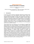
Dynamic models of the musculoskeletal system are typically comprised of four important
components: 1) the equations of motion for the body, or skeletal dynamics, 2) a representation
of musculoskeletal geometry, 3) a model of muscle-tendon mechanics, and 4) a model of
activation dynamics. Figure 1 illustrates how these components are combined to execute a
forward dynamic simulation. Basedv on a set of initial states, which include the muscle
v
v
activations, a (t ) , the muscle forces, f (t ) , the generalized speeds q& (t ) , and the generalized
v
coordinates, q (t ) , differential equations (See Eqs. (1)-(3) below) are used to compute the time
rate of change of the states. Then a numerical integration is performed to compute the states at
time t + dt . The new states are fed back and the forward dynamics process repeats, advancing
the states in time until the final time of the simulation is reached. In the simulations you will
conduct in this lab, a variable-step, 5-6, Runge-Kutta-Felberg integrator is used (Atkinson et al.,
1989).
Figure 1. Schematic of a forward dynamic simulation.
Skeletal dynamics
The equations of motion for the body allow one to compute the accelerations of the body
segments when forces and torques are applied to the body. The equations of motion can be
expressed as follows:
t v v
v v v
v v
v v v
v t v
q&& = I (q) −1 ⋅ {C (q , q& 2 ) + G( q) + R (q ) ⋅ f M + E (q ) ⋅ f E } .
(1)
Eq. (1) is simply an elaboration of Newton’s third law for a multi-link system, rearranged so that
v
−1
one can compute acceleration (i..e., a = m ⋅ f ). The vector of generalized coordinates, q ,vis
used
to specify
position and orientation of the segments of the body. The time derivatives of q ,
v&
v&
&
q and q , therefore represent the velocities and accelerations of the segments. Depending on
v
how one chooses to model the body, elements of q may be translational displacements,
2
orientations of segments with respect to the lab frame (segment angles), or orientations of
segments with respect to other segments (joint angles). Implicit in one’s choice of generalized
coordinates are one’s assumptions about the how the joints of the body function. For example,
one often models the hip joint as a three degree-of-freedom ball-and-socket joint, which requires
three generalized coordinates: flexion-extension (q1 ), ab-adduction (q2 ), and internal-external
t v
rotation (q3 ). The system mass matrix, I (q ) , characterizes the inertial properties of the body
(i.e., masses and moments of inertia). The remaining terms in Eq. (1) express the generalized
v v v2
forces or torques that act on the body. C (q , q& ) represents centripetal forces that arise from the
t v v
v v
R( q) ⋅ f M represents
angular velocities of the segments; G(q ) represents gravitational
forces;
v v v
the moments applied at the joints by the muscles, and E (q ) ⋅ f E represents external forces
t v
R(q) is a matrix of moment
applied to the body such as the ground reaction
force.
The
matrix
v
v v
arms that transform the muscle forces,v f M , into joint torques. The matrix E (q ) performs a
similar function for the external forces, f E .
For simple models, it is possible to derive the equations of motion by hand. However, for
more complex models, this is generally not feasible, and the equations of motion are generated
on a computer. The jumping model used in this lab has 23 degrees of freedom (Anderson and
Pandy, 1999), and the equations of motion for the jumping model were generated using SD/Fast,
a commercially available software package from Symbolic Dynamics, Inc. (Symbolic Dynamics,
Inc., 1996). In subsequent labs, you will use SD/Fast and SIMM (Software for Interactive
Musculoskeletal Modeling) with its Dynamics Pipeline to generate equations of motion for
models you develop (Delp et al., 1990).
Musculoskeletal geometry
Accurately representing the path of a muscle from its
origin to its insertion is one of the more challenging aspects of
modeling the musculoskeletal system. Sometimes a muscle can
be represented as a straight-line path between its origin and
insertion. Other times it is adequate to approximate the path as
a series of straight-line segments which pass through a series of
via points (Delp et al., 1990). When modeling muscle paths in
three dimensions, it is often necessary to simulate how muscles
wrap over underlying bone or musculature. Cylinders, spheres,
and ellipsoids have been used as wrapping surfaces (Van der
Helm et al., 1992; Garner and Pandy, 2000; Arnold et al.,
2000). The jumping model used in this lab uses cylindrical
wrapping surfaces to model the wrapping of gastrocnemius and
hamstrings around the femoral condyles, iliopsoas over the rim Figure 3. Path geometry of psoas.
of the pubic ramus, and gluteus maximus over underlying bone
and musculature. In Lab 2, you will use SIMM to specify, alter, and visualize musculoskeletal
geometry for a kinematic model you develop.
Muscle-tendon mechanics
The force producing properties of muscle are complex and nonlinear (See McMahon
(1984) for review) (Fig. 3). For simplicity, lumped-parameter dimensionless muscle models,
capable of representing a range of muscles with different architectures, are most commonly used
in dynamic simulation of movement (Zajac, 1989). In this lab, the jumping model is actuated by
54 musculotendinous units, each of which is represented as a Hill-type contractile element in
series with tendon. The parameters used to characterize each muscle are maximum isometric
M
M
T
force, Fo , optimal muscle fiber length, lo , tendon slack length, l S , maximum shortening
3
M
velocity, Vmax , and pennation angle, α . For a table of the muscle-tendon parameters, consult
Anderson and Pandy (1999). During a forward dynamic simulation, muscle force is treated as a
state and integrated forward in time using a first-order differential equation of the form
&f MT = Φ ( f MT , l MT , v MT , a) ,
(2)
MT
MT
MT
where f
,l
, and v
are the force, length, and velocity of the muscle-tendon actuator,
respectively, and Φ is a non-linear function (Zajac, 1989). In Lab 4, you will concentrate
specifically on modeling muscle.
l
l
l
l l
l
l l
l
Figure 3. Dimensionless model of muscle and tendon used in our simulations. Muscle properties are represented
by an active contractile element (CE) in parallel with a passive elastic element (top). Muscle force is dependent on
muscle fiber length (middle plot) and velocity (right plot). Muscle is in series with tendon, which is represented by
a nonlinear elastic element (left plot). Pennation angle (α) is the angle between the muscle fibers and the tendon.
The forces in muscle and tendon are normalized by peak isometric muscle force ( FoM ) . Muscle fiber length (l M ) and
tendon length (l T ) are normalized by optimal fiber length (loM ) . Tendon slack length (l ST ) is the length at which
tendons begin to transmit force when stretched. Velocities are normalized by the maximum contraction velocity of
M
muscle (Vmax
) . For a given muscle-tendon length (l MT ) , velocity, and activation level, the model computes muscle
M
force ( F ) and tendon force ( F T ) .
Activation dynamics
A muscle is not capable of generating force or relaxing instantaneously. The
development of force is a complex sequence of events which begins with the firing of motor
units and culminates in the formation of actin-myosin cross-bridges within the myofibrils of the
muscle. When the motor units of a muscle depolarize, action potentials are elicited in the fibers
of the muscle and cause calcium ions to be released from the sarcoplasmic reticulum. The
increase in calcium ion concentrations then initiates the cross-bridge formation between the actin
and myosin filaments (See Guyton (1986) for review). In isolated muscle twitch experiments,
the delay between a motor unit action potential and the development of peak force has been
observed to vary from as little as 5 milliseconds for fast ocular muscles to as much as 40 or 50
milliseconds for muscles comprised of higher percentages of slow-twitch fibers. The relaxation
of muscle depends on the re-uptake of calcium ions into the sarcoplasmic reticulum. This reuptake is a slower process than the calcium ion release, and so the time required for muscle force
to fall can be considerably longer than the time for it to develop.
In the forward dynamic simulations you will conduct in this lab, activation dynamics is
modeled using a first-order differential equation to relate the rate of change in activation (i.e., the
concentration of calcium ions within the muscle) to excitation (i.e., the firing of motor units):
4
a& =
( x 2 − xa ) ( x − a )
+
,
τ rise
τ fall
(3)
where a is the activation level of a muscle, x is the excitation level of a muscle, and τ rise and
τ fall are the rise and fall time constants for activation, respectively. In the model, activation is
allowed to vary continuously between zero (no contraction) and one (full contraction). In the
body, the excitation level of a muscle is a function both of the number of motor units recruited
and the firing frequency of the motor units. Some models for excitation-contraction coupling
distinguish these two control mechanisms (Hatze, 1976), but it is often not computationally
feasible to use such models when conducting complex dynamic simulations. In the jumping
model, the muscle excitation signal is assumed to represent the net effect of both motor neuron
recruitment and firing frequency, and, like muscle activation, is also allowed to vary
continuously between zero (no excitation) and one (full excitation). The rise and fall time
constants for muscle activation are assumed to be 22 and 220 milliseconds, respectively (Zajac,
1989).
IV.
Deliverables
At the completion of most labs you will need to turn in computer files from
you’remodeling and simulation work. They should be copied to /home/me382/username/L#,
where username is your workstation login name and # is a number corresponding to the lab your
working on (i.e., # = 1, 2, … for Labs 1, 2, …). You are the only person who will have read
and write permission to these directories during the week or two that a lab is in progress. In
addition, you will often be asked to turn in a written report summarizing your findings and
addressing questions which are posed as part of the lab.
Deliverables for Lab 1
1.
A 2-3 page written report
A Microsoft Word template for the report called lab1_report.doc is available on the BME
workstations in /software/nmbl/tutorials/me382/L1.
Deposit the following computer files to /home/me382/username/L1
2.
3.
V.
jcontrols.best
jcontrols.best.muscle
Excitation histories for your best-performance jump
Excitation histories for your best-performance jump without using a
particular muscle. Replace muscle in the name of the file with the
abbreviation of the muscle you did not excite (e.g.
jcontrols.best.HAMS ).
Input Files
1. /software/nmbl/tutorials/me382/L1/jinit.in
A file which specifies the initial values for the generalized coordinates, generalized
velocities, muscle forces, and muscle activations for the jumping simulation.
2. /software/nmbl/tutorials/me382/L1/jcontrols.stat
A muscle excitation file which will hold the jumping model in a static squat position.
3. /software/nmbl/tutorials/me382/L1/jmodel.gfrc.opt
A data file containing the ground reaction forces predicted by the dynamic optimization
solution.
5
VI.
Getting Started
Compute work
All labs for the class will be hands-on and require that you have your own user account
on the UNIX workstations in the BME computer lab. If you need an account, contact the
instructor. Each lab will guide you through a series of exercises which may require you to
execute certain commands. The commands you will need to execute are in Courier typeface.
Interactive dynamic simulator and muscle excitation editor
In this lab, you will use an interactive dynamic simulation program that allows you to edit
the excitation signals sent to the muscles. Before starting the program you will need to copy two
files to a directory which you make in your own home directory. Then, you can start the
simulator by typing the command jump.
#
#
#
#
#
#
mkdir L1
cd L1
cp /software/nmbl/tutorials/me382/L1/jcontrols.stat .
cp /software/nmbl/tutorials/me382/L1/jinit.in .
cp jcontrols.stat jcontrols
jump
jcontrols.stat contains excitation histories for the 54 muscles
The file
which will hold the
jumping model in a squat position. The dynamic simulator always looks for a file called
jcontrols, so it is necessary to copy jcontrols.stat to jcontrols. The file jinit.in contains the
initial states for the jumping simulation.
The simulator has two windows: the ExcitationEditor and the 3DView. When you type
jump , the ExcitationEditor comes up. Click the middle mouse inside the ExcitationEditor to
initialize it. After initialization, to the right of each muscle, you will see a series of nodes
connected by lines. Each line represents the excitation history for each muscle (i.e., x(t) in Eq.
3). The horizontal axis is time.
You can edit individual nodes or groups of nodes using the left mouse. Clicking the left
mouse on a node toggles the node back-and-forth from an unslected state (white) to a selected
state (red). When nodes are in a selected state, you can decrease or increase their excitation
levels by left clicking on any selected node and dragging the mouse down or up. You can select
a group of nodes by clicking the left mouse in an open area (i.e., not on a node) and dragging the
left mouse to form a rectangle. All nodes within the rectangle will become selected. You can
deselect or clear all nodes by clicking the middle mouse button.
Excitation Editor Command Summary
select/deselect a node
select a group of nodes
decrease/increase excitation
clear all selected nodes
integrate
save controls to file jcontrols.new
quit
forced quit without saving
left mouse click
in open space
left mouse drag of selected node(s)
left mouse drag
middle mouse click
in left column
left mouse click on SAVE
left mouse click on QUIT
shift + left mouse click on QUIT
right mouse click
To begin an integration, click the right mouse in the blue area of any of the excitation
fields on the left side of the ExcitationEditor. The first time you request an integration, the
3DView will appear and display the model in its initial position. As the integration progresses, a
vertical white line will trace across the ExcitationEditor from left to right indicating the current
time of the integration. As the integration passes each node, the states are stored so that
6
subsequent integrations can start from any node which has associated with it a valid set of states.
A vertical black line indicates the most advanced node from which an integration can be started.
To start an integration from a particular node, right mouse click just to the right of the node. For
example, if you want to integrate starting the beginning, right mouse click to the right of the first
node; if you want to integrate from the third node, right click to the right of the third node.
At any time you can save your edited controls by left clicking the SAVE button in the lower left
corner of the ExcitationEditor. This will write your controls to a file called jcontrols.new. If
you wish to start up the dynamic simulator from a saved control files it is necessary to quit the
simulator (left click the QUIT button), copy the saved controls file to jcontrols, and restart
the simulator.
The 3DView allows you to view the musculoskeletal model as an integration executes.
The long red cylindrical shapes represent the paths of muscles. The activation level of a muscle
is proportional to the intensity of red with which its path is drawn. The joint axes of the model
are shown as short blue arrows. The magnitude and direction of the ground reaction forces
applied to the feet are displayed as green vectors applied at five locations under each foot. Each
of the five locations corresponds to a location at which a spring and damper force is applied (see
Anderson and Pandy (1999) for details).
It is possible to rotate and translate the 3DView to obtain different perspectives on the
model (Table 2). With respect to the computer screen, the x, y, and z axes of the window are up,
to the right, and out of the screen, respectively. To interrupt the integration and return to the
ExcitationEditor, you can type the ESC key while the mouse pointer is within the 3DView
window.
BUG Note that if you attempt to control the 3DView while the 3DView window is not
integrating, the dynamic simulator will lock up and you will have to type <CNTRL>C to exit the
simulator.
Table 2: 3DView Commands
left mouse drag left and right
left mouse drag up and down
Z_Key+left mouse drag up and down
middle mouse drag left and right
middle mouse drag up and down
Z_Key+middle mouse drag up and down
ESC_Key
Rotate about window y axis (vertical axis)
Rotate about window x axis (horizontal axis)
Rotate about window z axis (out of the screen)
Translate along window x axis (horizontal axis)
Translate along window y axis (vertical axis)
Translate along window z axis (out of the screen)
Interrupt integration and return to ExcitationEditor
NOTE For this lab, it is assumed that the muscles on the left and right sides of the body are
excited symmetrically. You must therefore make all your changes to the muscle excitation
histories on the left side of the ExcitationEditor. You will notice that as you make changes to the
left side excitations, they are mirrored on the right side of the ExcitationEditor.
VII.
Muscular Control Strategies for Maximizing Jump Height
Following are a series of tasks for you to perform and questions for you to answer. The answers
to the questions constitute your written report for Lab 1. For a list of muscle abbreviations used
in this lab, see Table III in Anderson and Pandy (1999).
1. Starting from the static controls (i.e., # cp jcontrols.stat jcontrols), use the left mouse
button to select all the nodes for VAS. Then, by dragging one of the selected nodes upward with
the left mouse, increase the excitation of all nodes to maximum. Then, start a forward
integration by clicking the right mouse in one of the blue excitation fields on the left-hand side of
7
the ExcitationEditor. Let the integration complete. Briefly describe the effect of exciting VAS
on the joint angles and the ground reaction force.
2. Why does a force in VAS, which is a uniarticular knee extensor, accelerate joints it does not
span? Explain this dynamic coupling both physically and in terms of the inertia matrix of Eq.
(1)?
3. Quit the ExcitationEditor (shift + left mouse click on QUIT) and restart the program to
reload the static equilibrium controls. Repeat exercise 1 above for SOL.
4. … for GAS.
5. … for GMAXM and GMAXL together.
6. … for HAMS.
7. … for ADM.
8. By manually editing the muscle excitation histories, find a set of muscle excitation patterns
which produce a well coordinated jump. Try to maximize overall performance which is jump
height minus ligament force penalties. Jump height for the model is defined as the height
reached by the center of mass above the model’s standing height in meters. The ligament
penalty is the integral of ligament joint torques over the duration of the simulation multiplied by
a constant (See Anderson and Pandy (1999) for details. The performance numbers will print out
in your command shell as an integration progresses. Record your best performance numbers in
your written report, and make sure to save the corresponding set of controls to file (left
mouse click on SAVE, then in the UNIX shell, # cp jcontrols.new jcontrols.best).
ligament penalty =
jump height =
overall performance =
9. If you are able to get the model to jump anywhere near the jump height predicted by the
optimal solution (i.e., over 1.41 meters), you should be congratulated. It is not easy to do. In the
more likely event that your solution was not as high as the optimal solution, explain why.
11. Before you started on the lab, you should have been assigned a muscle (e.g., SOL, HAMS,
VAS, …). Now, as you did in exercise 8, make the model jump as high as possible without
using this muscle. Make sure to save the controls corresponding to your best performance
to file (see the Deliverables section above). What is the performance difference between this
jump and your best jump when you could use all the muscles? What would you infer is the
function of this muscle during jumping?
VIII. Analyses
You will now take a brief look at some of the data which is available from your
simulation. First, you will need to generate the data. Execute the following commands:
# cp jcontrols.best jcontrols
# jumpData
The following files should be generated:
model.gfrc
Time history of the ground reaction force (sum of spring forces)
model.jfrc
Time history of the articular contact forces at the joints
model.mexc
Time history of muscle excitations
model.matv
Time history of muscle activations
8
model.mfrc
Time history of muscle forces
1. Plot the vertical ground reaction force predicted by your solution and by the optimal solution.
Include this plot in your report. The ground reaction forces for the optimal solution are in the
file jmodel.gfrc.opt which you can find in /software/nmbl/tutorials/me382/L1. Does
your ground reaction force have a higher or lower peak? Is the time to lift-off longer or shorter?
2. Plot the resultant articular contact force at the hip as a percentage of body weight. Include this
plot in your written report. Why are the hip contact forces are so large?
3. On a plot, superimpose the excitation levels, activation history, and force history predicted by
your solution for VAS. Include this plot in your written report. Given what you know about
muscle mechanics, explain why the force generated by VAS was less than its isometric strength?
IX.
Stepping through the Code
Now that you have an idea of how a dynamic musculoskeletal model can be used, take a
look at the computer code that was used to generate the simulation programs you have been
using. To do this, you will use the SGI debugger to step through the code. Also available to you
are some hardcopy printouts of some routines which should have been distributed with this lab.
This exercise is an opportunity to begin getting familiar with dynamic simulation code and also
an opportunity to start learning the debugger, which will be useful when you build your own
dynamic models.
Note that before this lab is due there will be a lecture in which the structure of the code is
reviewed. At your discretion you can wait until after that lecture to step through the code.
However, you are encouraged to take at least a short look at the code and the debugger before
that lecture so that you know what the code looks like and so that you might formulate some
questions.
The cvd debugger
The SGI debugger is called cvd. If you are familiar with dbx, a standard debugger on
most UNIX systems, you will already be familiar with the basic workings of cvd. cvd is a more
capable, graphical version of dbx . To use cvd on an executable named myexe enter the
following command
# cvd myexe
The cvd user interface will come up displaying the text code for the entry point of myexe. To
step through the code successfully, myexe needs to have been compiled with the –g option:
# cc –g –o myexe myexe.c
The –g option preserves the symbols of myexe.c and prevents the compiler from performing
optimization and reordering execution steps. You can find help for cvd in the Irix man pages
(type man cvd at the Unix shell command prompt). Since the commands in cvd are based on
dbx, the dbx man pages will also be useful (type man dbx).
For this lab
Step through the simulation code by typing the command
# jumpDataDebug
The cvd debugger will start and show the main program for the jumping code. Place a STOP in
the main program by left clicking the mouse in the left margin. Start execution by clicking the
Run button in the upper right hand corner of the cvd debugger window, or by typing rerun in the
command window at the bottom of the main window. Once the process is executing, you can
step through the code using the cvd buttons or by entering commands in the lower command
window. Consult the dbx man pages for the basic commands.
9
You should step down into the code deep enough that you go through the integrator and
execute lines of code in ydot23(). You do not need to include anything in your report from this
exercise.
A note regarding how the cvd debugger was started for this exercise--The programs you have been running were actually started with script files, so executing the
command
# cvd jumpData
would NOT have worked with cvd because jumpData is only a script file. To invoke the
debugger on jumpData, the script file jumpDataDebug was created which internally starts the
cvd debugger.
X.
References
Anderson FC and Pandy MG (1999). A dynamic optimization solution for jumping in three
dimensions. Computer Methods in Biomechanics and Biomedical Engineering, 2, 201-231.
Arnold AS, Salinas S, Asakawa DJ, Delp SL (2000). Accuracy of muscle moment arms
estimated from MRI-based musculoskeletal models of the lower extremity. Computer Aided
Surgery, 5, 108-119.
Atkinson LV, Harley PJ, Hudson JD (1989). Numerical methods with FORTRAN 77. AddisonWesley Publishing Company, Menlo Park.
Delp SL, Loan JP, Hoy MG, Zajac FE, Topp ET, Rosen JM (1990). An interactive graphicsbased model of the lower extremity to study orthopaedic surgical procedures. IEEE
Transactions in Biomedical Engineering, BME-37, 757-767.
Garner BA, Pandy MG (2000). The obstacle-set method for representing muscle paths in
musculoskeletal models. Computer Methods in Biomechanics and Biomedical Engineering, 3, 130.
Guyton AC (1986). Textbook of medical physiology, Seventh Edition. W. B. Saunders
Company, Philadelphia.
Hatze H (1976). The complete optimization of human motion. Mathematical Biosciences, 28,
99-135.
McMahon TA (1984). Muscles, Reflexes, and Locomotion. Princeton University Press,
Princeton, New Jersey.
Symbolic Dynamics, Inc. (1996). SD/FAST User’s Manual, Version B.2. Mountain View, CA.
Van der Helm FCT, Veeger HEJ, Pronk GM, Van der Woude LHV, Rozendal RH (1992).
Geometry parameters for musculoskeletal modeling of the shoulder system. Journal of
Biomechanics, 2, 129-144.
Zajac FE (1989). Muscle and tendon: properties, models, scaling, and application to
biomechanics and motor control. CRC Critical Reviews in Biomedical Engineering (Edited by
Bourne JR), 17, 359-411. CRC Press, Boca Raton.
10