Download PACS Observer`s Manual

Announcement of Opportunity for Key Programmes
PACS Observer's Manual
HERSCHEL-HSC-DOC-0832, Version 1.5
17-October-2007
PACS Observer's Manual
Published version 1.0, 01 February 2007
Published version 1.1, 14 March 2007
Published version 1.2, 04 June 2007
Published version 1.3, 04 July 2007
Published version 1.4, 08 October 2007
Published version 1.5, 17 October 2007
Published
Table of Contents
1. Introduction ...................................................................................................................... 1
1.1. Purpose of document ................................................................................................ 1
1.2. Background ............................................................................................................ 1
1.3. Acknowledgements ................................................................................................. 2
1.4. Acronyms .............................................................................................................. 2
2. The PACS instrument ......................................................................................................... 3
2.1. Overview: instrument concept ................................................................................... 3
2.2. Common Optics ...................................................................................................... 5
2.2.1. Entrance Optics ............................................................................................ 5
2.2.2. Calibration sources ........................................................................................ 5
2.2.3. Chopper ...................................................................................................... 6
2.3. Photometer ............................................................................................................ 6
2.3.1. Filters ......................................................................................................... 6
2.3.2. Bolometer arrays .......................................................................................... 7
2.3.3. Cooler ........................................................................................................ 8
2.4. Spectrometer .......................................................................................................... 8
2.4.1. Image slicer ................................................................................................. 8
2.4.2. Grating ....................................................................................................... 9
2.4.3. Order sorting Filters .....................................................................................10
2.4.4. Photoconductor arrays ..................................................................................10
3. Scientific capabilities .........................................................................................................12
3.1. Herschel telescope ..................................................................................................12
3.2. Chopper ...............................................................................................................12
3.3. Mirrors .................................................................................................................13
3.4. Characteristics of the photometer ..............................................................................13
3.4.1. Photometer spatial resolution .........................................................................13
3.4.2. Photometer filters ........................................................................................14
3.4.3. Photometer bad pixels ...................................................................................16
3.4.4. Photometer sensitivity ..................................................................................16
3.5. Characteristics of the spectrometer ............................................................................18
3.5.1. Diffraction Losses ........................................................................................18
3.5.2. Grating efficiency ........................................................................................18
3.5.3. Spectrometer filters ......................................................................................18
3.5.4. Spectrometer spatial resolution .......................................................................19
3.5.5. Spectrometer spectral resolution .....................................................................20
3.5.6. Spectrometer relative spectral response function ................................................21
3.5.7. Spectrometer sensitivity ................................................................................22
4. Observing with PACS ........................................................................................................25
4.1. PACS photometer AOT ...........................................................................................25
4.1.1. Point-source photometry ...............................................................................26
4.1.1.1. Chopper avoidance angle in point-source mode .......................................28
4.1.2. Small-source photometry ...............................................................................29
4.1.2.1. Chopper avoidance angle in small-source mode ......................................29
4.1.3. Large area or extended source mapping ............................................................31
4.1.3.1. Raster mapping mode .........................................................................32
4.1.3.1.1. Raster map orientation constraint ...............................................33
4.1.3.2. Scan mapping mode ...........................................................................34
4.1.3.2.1. Scan maps in instrument reference frame .....................................35
Scan map orientation ....................................................................36
4.1.3.2.2. Scan maps in sky coordinates ....................................................37
4.1.3.3. Scan maps sensitivity .........................................................................40
4.1.4. Gain setting for bright sources ........................................................................40
4.2. PACS spectrometer AOTs .......................................................................................42
4.2.1. Line scan spectroscopy AOT ..........................................................................42
4.2.1.1. Standard chopping-nodding mode ........................................................43
4.2.1.2. Bright lines chopping-nodding mode .....................................................45
4.2.1.3. Line scan in wavelength-switching mode ...............................................45
iii
PACS Observer's Manual
4.2.2. Range scan spectroscopy Mode ......................................................................47
4.2.2.1. Raster mapping in range scan ..............................................................47
4.2.2.2. Range scan .......................................................................................48
4.2.2.3. SED mode .......................................................................................49
5. Calibration framework .......................................................................................................51
6. Using HSpot to create PACS observations .............................................................................52
6.1. Guidelines to AOT use ............................................................................................52
6.2. Tutorial of an AOT entry in HSpot ............................................................................52
6.2.1. Tutorials of Photometer AOT entry .................................................................52
6.2.1.1. Tutorial of point-source photometry mode entry ......................................53
6.2.1.2. Example of a raster map entry ..............................................................59
6.2.1.3. Tutorial of Photometer scan map entry ..................................................64
6.2.2. Tutorials of Spectrometer AOT entry ...............................................................67
6.2.2.1. Example of line spectroscopy AOT entry ...............................................68
6.2.2.2. Example of range spectroscopy AOT entry .............................................73
7. Pipeline description and data product expectations ..................................................................80
7.1. PACS photometry standard data processing .................................................................80
7.1.1. Photometry processing steps ..........................................................................80
7.1.2. Photometer processing levels .........................................................................81
7.1.3. Photometer processing flow diagram ...............................................................81
7.2. PACS spectrometry standard data processing ...............................................................88
7.2.1. PACS spectrometry processing steps ...............................................................88
7.2.2. Spectrometer processing levels .......................................................................88
7.2.3. Spectrometer processing flow diagram .............................................................89
8. Change record ..................................................................................................................95
References ..........................................................................................................................97
iv
Chapter 1. Introduction
1.1. Purpose of document
The PACS Observer's manual is intended to support astronomers to in the definition of their observations with the PACS instrument. The purpose of this document is to provide relevant information
about the PACS instrument on board Herschel Space Observatory. The information is mainly targeted to be a general overview of the instrument and its performance, in order to help the astronomer to plan, prepare and execute scientific observations with PACS.
The structure of this observer's manual is as follows: we first describe the instrument (Chapter 2)
and its scientific capabilities (Chapter 3), followed by the available astronomical observation templates (AOTs, Chapter 4). The calibration scheme and products are presented in Chapter 5. A cookbook for entering observations with HSPOT is given in Chapter 6 and the manual ends with a description of the pipeline (Chapter 7).
This version is written to support the 2007 Open Time - Key Programmes call for Herschel observing proposals by the European Space Agency (ESA).
Note
The Herschel Observers' Manual provides further information about Herschel pertinent to using the
observatory from the perspective of an observer.
1.2. Background
The Herschel Space Observatory is an ESA cornerstone mission, for high spatial resolution observations in the FIR and sub-millimeter regime, to be launched in 2008 aboard an Ariane 5 rocket together with Planck. It will enter a Lissajous 700 000 km diameter orbit 1.5 million kilometers away
from Earth at the second Lagrange point of the Earth-Sun system.
The mission is named after Sir William Herschel, who discovered the infrared radiation in 1800.
It will be the first space observatory to cover the full far-infrared and submillimetre waveband. It
will perform photometry and spectroscopy in the 55-670 µm range, with its 3.5m diameter radiatively cooled telescope, while its science payload complement of three instruments is housed inside a
superfluid helium cryostat.
Herschel is designed to observe the "cool universe". The main scientific objectives of the mission
are:
•
to study the formation of galaxies in the early universe and their subsequent evolution;
•
to investigate the formation of stars and their interaction with the interstellar medium;
•
to observe the chemical composition of the atmospheres and surfaces of comets, asteroids, planets and satellites;
•
to examine the molecular chemistry of the universe.
Herschel will be operated as an observatory facility offering three years of routine observations,
which will be available for the entire scientific community. Roughly two thirds of the observing
time are "open time", and will be offered through a standard competitive proposal procedure.
The Photodetector Array Camera & Spectrometer (PACS) is one of the three science instruments of
the Herschel observatory. PACS provides the Herschel Space Telescope with the capabilities for
spectroscopy and imaging/photometry in the 55-210 µm range.
1
Introduction
PACS has been designed and built by a consortium of institutes and university departments from
across Europe under the leadership of the Principal Investigator Albrecht Poglitsch at MaxPlanck-Institute for Extraterrestrial Physics, Garching, Germany. Consortium members are from
Austria: UVIE; from Belgium: IMEC, KUL, CSL; from France: CEA, OAMP; from Germany:
MPE, MPIA; from Italy: IFSI, OAP/OAT, OAA/CAISMI, LENS, SISSA; from Spain: IAC.
The PACS web site is : http://pacs.mpe.mpg.de
1.3. Acknowledgements
The PACS instrument is the result of many years of work by a large group of dedicated people in
several institues and companies across Europe. It is their efforts that have made it possible to create
such a powerful instrument for use in the Herschel Space Observatory. We would first like to acknowledge their work.
This manual is edited by Bruno Altieri and Roland Vavrek (ESAC) and includes help and inputs
from a number of people. Particular help and contributions to this manual have come from Ulrich
Klaas, Thomas Müller, Marc Sauvage, Jürgen Schreiber, Eckhard Sturm and Bart Vandenbussche.
This Observer's Manual also uses the knowledge contained in numerous PACS technical documents
and various discussions.
1.4. Acronyms
• AOR : Astronomical Observation Request
• AOT : Astronomical Observation Template
• CRE : Cryogenic Readout Electronics
• DDCS : Double Differential Correlated Sampling (mode)
• DMC : Detector and Mechanics Controller
• DTCP : Daily TeleCommunications Period
• ESA : European Space Agency
• FM : Flight Model
• FOV : Field-Of-View
• FPU: Focal Plane Unit
• FWHM : Full Width Half Maximum
• HSpot: Herschel planning observations tool
• ICC: Instrument Control Centre
• ICS: Internal Calibration Source
• ILT: Integrated (Instrument) Level Tests
• NEP: Noise Equivalent Power
• OD: Observation Day
• PACS : Photodetector Array Camera & Spectrometer
• QLA : Quick Look Analysis
• QM: Qualification Model
• RSRF: Relative Spectral Response Function
• SED: Spectral Energy Distribution
• SPU: Signal Processing Unit
2
Chapter 2. The PACS instrument
2.1. Overview: instrument concept
The PACS instrument comprises two sub-instruments which offer two basic and and mutually exclusive modes in the wavelength band 55-210 µm :
•
Imaging dual-band photometry (60-85 µm or 85-130 µm and 130-210 µm) over a field of view
of 1.75'x3.5', with full sampling of the telescope point spread function (diffraction/wavefront error limited)
•
Integral-field spectroscopy between 55 and 210 µm with a resolution of ~75-300km/s and instantaneous coverage of ~1500 km/s, over a field of view of 47"x47".
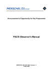
Figure 2.1. Left: Optical layout. After the common entrance optics with calibration sources and the
chopper, the field is split into the spectrometer train and the photometer trains. In the latter a dichroic
beam splitter feeds separate re-imaging optics for the two bolometer arrays. In the spectrometer train,
the image slicer converts the square field into an effective long slit for the Littrow-mounted grating spectrograph. The dispersed light is distributed to the two photoconductor arrays by a dichroic beam splitter
which acts as an order sorter for the grating.
Figure 2.1 shows how the functional groups are distributed in the spatial instrument envelope.
Figure 2.2 shows an optical circuit block diagram of the major functional parts of PACS. At the top,
3
The PACS instrument
the entrance and calibration optics is common to all optical paths through the instrument. On the
right, the spectrometer serves both, the short-wavelength (“blue”), and long-wavelength (“red”) photoconductor arrays. A fixed dichroic beam splitter separates blue from red spectrometer light at the
very end of the optical path. On the left, the bolometer fixed dichroic beam splitter comes before the
blue and red imaging branches since they require different magnification. Directly in front of their
baffle enclosures the blue detectors have filter wheel mechanisms which contain the band pass filters for short wavelength photometry, and the order selection band passes for 2nd and 3rd order operation of the grating spectrometer, respectively.
Figure 2.2. Functional block diagram of PACS overall optics
The focal plane sharing of the instrument channels is shown in Figure 2.3. The photometric bands,
which can be observed simultaneously, cover the same field-of-view. The field-of-view of the spectrometer is offset from the photometer field (see Figure 2.3). However, this has no effect on the observing efficiency.
The focal plane unit provides photometric and spectroscopic capabilities through five functional
units :
•
common input optics with the chopper, calibration sources and a focal plane splitter;
•
a photometer optical train with a dichroic beam splitter and separate re-imaging optics for the
two short-wavelength bands (60-85 µm/ 85-130 µm) selectable via a filter wheel and the longwavelength band (130-210 µm), respectively;
•
two bolometer arrays with cryogenic buffers/multiplexers and a common 0.3 K sorption cooler;
•
a spectrometer optical train with an image slicer unit for integral field spectroscopy, an anamorphic collimator, a movable diffraction grating in Littrow mount, anamorphic re-imaging optics, and a dichroic beam splitter for separation of diffraction orders. The blue channel contains
an additional filter wheel for selecting its short or long wavelength part;
•
two photoconductor arrays with attached cryogenic readout electronics (CRE).
4
The PACS instrument
PACS focal plane usage. Long-wavelength and short wavelength photometry bands cover practically identical fields-of-view. The spectrometer FOV is offset in the -Z direction (closer to the optical
axis of the telescope). Chopping is done along the Y axis (left-right in this view) and also allows observation of the internal calibrators on both sides of the used area in the telescope focal plane. The
maximum chopper throw for sky observations is ~3.5 arcmin for photometry and 6.3 arcmin for
spectroscopy. In photometry, object and reference fields are almost touching at 3.5 arcmin throw.
Figure 2.3. PACS field-of-view footprint in the telescope focal plane.
2.2. Common Optics
2.2.1. Entrance Optics
The entrance optics fulfills the following tasks: it creates an image of the telescope secondary mirror
(the entrance pupil of the telescope) on the focal plane chopper; this allows spatial chopping with as
little as possible modulation in the background received by the instrument.
It also provides for an intermediate pupil position where the Lyot stop and the first blocking filter,
common to all instrument channels, can be positioned. It allows the chopper, through two field mirrors adjacent to the used field of view in the telescope focal surface, to switch between a (chopped)
field-of-view on the sky and two calibration sources (see also Figure 2.3).
The chopped image is then re-imaged onto an intermediate focus where a fixed field mirror splits off
the light into the spectroscopy channel. The remaining part of the field of view passes into the photometry channels. A "footprint" of the focal-plane splitter is shown in Figure 2.3.
2.2.2. Calibration sources
The calibration sources are placed at the entrance of the instrument to have the same light path for
the sky observation and internal calibration. This is essential for removing detector baseline drifts as
best as possible, a serious task with a warm telescope and the associated high thermal background.
To eliminate non-linearity or memory problems with the detector/readout system, the calibration
sources are low emissivity gray-body sources providing FIR radiation loads slightly above and be5
The PACS instrument
low the telescope background, respectively. This is achieved by diluting the radiation from a (small)
black source with a temperature near the telescope temperature inside a cold diffusor sphere with a
(larger) exit aperture. The temperature of the radiator (~80K) is stabilized within a few mK.
2.2.3. Chopper
In order to discriminate faint signals of celestial sources from orders of magnitude larger thermal
background fluxes of the only moderately cooled Herschel telescope (~80K), differential measurements are required. For this purpose a small tilting mirror, the chopper, flips alternately on the astronomical source and on a nearby sky position, with a variable throw up to 6 arcmin on the sky for the
spectrometer and 3.5 arcmin for the photometer. This allows full separation of an object field and a
reference field.
The chopper is also used to alternatively look at the two internal calibration sources (ICS) which are
located at the left and right side of the instrument FOV (see Figure 2.3).
The chopper is capable of following staircase waveforms with a resolution of 1", and delivers a
duty-cycle of ~90% at chop frequency of 5 Hz. The chopper axis is stabilized in its central position
by flexular pivots and rotated by a linear motor. The chopper design allows a low heat load in the
PACS FPU.
At larger elongations the chopper is used to reflect the beams from the ICSs within the PACS Focal
Plane Unit enabling frequent photometric calibration of the detector arrays during the flight.
2.3. Photometer
After the intermediate focus provided by the entrance optics, the light is split into the longwavelength and short-wavelength channels by a dichroic beam-splitter with a transition wavelength
of 130 µm and is re-imaged with different magnification onto the respective Si bolometer arrays.
The blue channel offering two filters, 60-85 µm and 85-130 µm, has a 32x64 pixels arrays, while the
red channel with a 130-210 µm filter has a 16x32 pixels array. Both channels cover a field-of-view
of ~1.75'x3.5', with full beam sampling in each band. The two short-wavelength bands are selected
by two filters via a filter wheel. The field-of-view is nearly filled by the square pixels, however the
arrays are made of sub-arrays which have a gap of ~1 pixel in-between.
The incident infrared radiation is registered by each bolometer pixel by causing a tiny temperature
difference.
2.3.1. Filters
The PACS filters, in combination with the detectors, define the photometric bandpass of the instrument. There are in total 3 bands in the PACS photometer: 60-85 µm, 85-130 µm and 130-210 µm.
The transmission of the photometer filters is shown in Figure 3.4.
6
The PACS instrument
Figure 2.4. Overview of the filter arrangements in PACS. The selection of the blue photometer filter is
done via commanding of the filter wheel 2.
2.3.2. Bolometer arrays
Figure 2.5 shows a cut-out of the 64x32 pixel bolometer array assembly. 4x2 monolithic matrices of
16x16 pixels are tiled together to form the short-wave focal plane array.
Figure 2.5. Bolometer matrices assembly: 4x2 matrices from the focal plane of the short-wave bolometer
assembly. The 0.3 K multiplexers are bonded to the back of the sub-arrays. Ribbon cables lead to the 3K
buffer electronics.
In a similar way, 2 matrices of 16x16 pixels, are tiled together on for the long-wavelength focal
plane array.
The matrices are mounted on a 0.3K carrier which is thermally isolated from the surrounding 2K
structure. The buffer/multiplexer electronics is split in two levels; a first stage is part of the indiumbump bonded back plane of the focal plane arrays, operating at 0.3K. Ribbon cables connect the output of the 0.3K readout to a buffer stage running at 2K.
7
The PACS instrument
For science observations the multiplexing readout samples each pixel at a rate of 40 Hz Because of
the large number of pixels, data compression by the SPU is required. The raw data are therefore
binned to an effective 10 Hz sampling rate. After that, the same lossless compression algorithm is
applied as with the spectrometer data.
2.3.3. Cooler
The photometer operates at sub-Kelvin temperatures, which are achieved using a 3He cooler. This
type of refrigerator uses porous material which absorbs or releases gas depending on the mode:
cooling or heating. The use of the 3He isotope instead of the common 4He is dictated by two reasons:
it is not super fluid at cryogenic temperatures below 2.2 K and it is a superior cryogen. This sorption
cooler is run from a cold stage provided by the Herschel cryostat. The refrigerator contains 6 litres
of 3He and can in principle be recycled infinitely, with an efficiency of more than 95% with a lifetime limited only by the cold stage from which it is run. Gas-gap heat switches, which are coupled
to the Herschel 3K system with thermal straps, control the mode of operations. The evaporation of
3
He provides a very stable thermal environment under constant heat load. The design of the cooler is
well suited for work in space as there are no moving parts and the heat load is small.
This sorption cooler is nearly identical to the unit developed for SPIRE. It provides a stable temperature environment at 300 mK for more than 48 hours under normal observing and operational circumstances. The recycling shall be performed during DTCP periods, whenever the PACS photometer will be selected for the following observing day.
2.4. Spectrometer
The spectrometer covers the wavelength range from 55µm to 210µm, in two channels that operate
simultaneously in the blue (55-98µm) and red (102-210µm) band. It provides a resolving power
between 1000 and 5000 (i.e. a spectral resolution of ~75-300km/s), depending on wavelength for a
fixed grating position The instantaneous coverage is ~1500km/s. It allows simultaneous imaging of
a 47"x47" field of view, resolved in 5x5 pixels. An image slicer employing reflective optics is used
to re-arrange the 2 dimensional field-of-view along a 1x25 pixels entrance slit for the grating, as
schematically shown in Figure 2.3.
This integral-field concept allows efficient detection of weak individual spectral lines with sufficient
baseline coverage and high tolerance to pointing errors without compromising spatial resolution, as
well as for spectral mapping of extended sources regardless of their intrinsic velocity structure.
The grating is Littrow-mounted, i.e. the entrance and exit optical paths coincide. It is operated in
first, second or third order, respectively, to cover the full wavelength range. The first order covers
the range 102-210µm, the second order 72-98µm, and the third order 55-72µm. Anamorphic collimating optics expands the beam to an elliptical cross section to illuminate the grating over a length required to reach the desired spectral resolution. The grating is actuated by a cryogenic motor with
arcsec precision which allows spectral scanning/stepping for improved spectral flat-fielding and for
coverage of extended wavelength ranges.
The light from the first diffraction order is then separated from the light of the two other orders by a
dichroic beamsplitter and passed into two optical trains feeding the respective detector arrays
(stressed/unstressed) for the wavelength ranges 102-210µm and 55-102µm. Anamorphic re-imaging
optics is employed to independently match the spatial and spectral resolution of the system to the
square pixels of the detector arrays. the filter wheel in the short-wavelength path selects the second
or third grating order.
2.4.1. Image slicer
The image slicer's main function is to transform the 5x5 pixel image at its focal plane into a linear
1x25 pixel entrance slit for the grating spectrometer. The slicer assembly consists of 3 set of mirrors:
•
The slicer stack: 5 identical spherical field mirrors, individually tilted, which forms separate pu8
The PACS instrument
pil images for each "slice" on the set of 5 capture mirrors.
•
The capture mirrors re-combine the separate beams into the desired linear image on the set of 5
spherical mirrors at the exit of the slicer assembly.
•
The field mirrors at the exit re-combine the pupils separated in the slicer into a common virtual
pupil. The collimators of the spectrometer will later form an (anamorphic) image of this virtual
pupil onto the grating. At the same time, the field mirror apertures serve as the entrance slit of
the grating spectrometer.
Figure 2.6. Integral-field spectrometer concept : projection of the focal plane onto the detector arrays in
spectroscopy mode. The image slicer re-arranges the 2D field along the entrance slit of the grating spectrograph such that, for all spatial elements in the field, spectra are observed simultaneously. Note the
blank space left between the slices to reduce crosstalk between left- and rightmost pixels of adjacent
slices (see also Figure 2.8 )
2.4.2. Grating
The grating blank has a length of 320mm with a groove period of 8.5 ±0.05 grooves/mm, with a
total of approximatively 2720 grooves. The reflection grating is operated in the first (102-210 µm),
the second (72-98 µm) and the third diffraction order (55-72 µm). Grating deflections from 25 de9
The PACS instrument
grees to 70 degrees are possible to cover the full wavelength range of each order. A graphical correlation of the grating angle of incidence versus order and wavelength is given in Figure 2.7.
Figure 2.7. Relation between grating angle and wavelength
2.4.3. Order sorting Filters
The PACS order sorting filters enable the spectral purity of the selected band by suppressing contributions by other orders the detector is sensitive to. There are in total 3 bands in the PACS spectrometer: 55-72 µm, 72-102 µm and 102-210 µm. The filter transmission is shown in Figure 3.8. The
filter train of both the photometer and spectrometer channels is illustrated in Figure 2.4.
2.4.4. Photoconductor arrays
The spectrometer employs two Ge:Ga photoconductors arrays (low and high stressed) with 16x25
pixels on which the 16 spectral elements of the 25 spatial pixels are imaged.
The Ge:Ga photoconductor arrays have a modular design : They are made of 25 linear modules of
16 pixels each are stacked together to form a 2-dimensional array. Ge:Ga photoconductors are sensitive in the wavelength range 40-110/120 µm without any stress. A stress is therefore applied to improve the long wavelength sensitivity. The stressing mechanisms ensures homogeneous stress on
each pixel along the entire pile of 16 spectral elements. The low-stressed has a mechanical stress on
the pixels which is reduced to about 10% of the level needed for the long-wavelength response.
Light cones in front of the actual detector block provide an area-filling light collection in the focal
plane and feed the light into the individual integrating cavities around each individual, mechanically
stressed detector crystal. The light cones also act as a very efficient means of straylight suppression
because their solid angle acceptance is matched to the re-imaging optics such that out-of-beam light
is rejected.
10
The PACS instrument
Figure 2.8. High stress module close-up : The 25 stressed modules (corresponding to 25 spatial pixels) integrated into their housing. Stress is applied to the whole stack of 16 Ge crystals, providing the instantaneous spectral coverage for each of the 25 spatial fields on the sky. Light cones provide for area-filling collection onto the individual detectors.
Each module is attached to a 18 channel cold readout electronics (CRE) amplifier/multiplexer circuit in CMOS technology. The photocurrent from the detector crystals is integrated on a capacitor.
The capacitance is switchable between 4 values from 0.1 to 3pF to provide sufficient dynamic range
for the expected flux range. The integration process is reset after preset interval. During the integration the voltage signal is regularly read in a non-destructive way with a frequency of 1/256s leading
to an integration ramp with 256 / (reset interval) samples.
11
Chapter 3. Scientific capabilities
Based on the results from the QM Instrument Level Tests, tests of FM components/subunits and our
present knowledge of the Herschel satellite, the performance of the entire system can be estimated in
terms of what the observer is concerned with, i.e., an assessment of what kind of observations will
be feasible with Herschel/PACS, and how much observing time they will require.
The system sensitivity of the instrument at the telescope depends mainly on the optical efficiency,
i.e. the fraction of light from an astronomical source arriving at the telescope that actually reaches
the detector, on the photon noise of the thermal background radiation from the telescope or from
within the instrument, and on detector/electronics noise.
3.1. Herschel telescope
Ideally, the telescope would be diffraction limited over the full PACS wavelength range. The
present telescope design allows a wavefront error of 6µm (r.m.s.). The type of error is not known;
we have assumed spherical aberration for the analysis. The main effect on the point spread function
(PSF) is a transfer of power from the central peak to larger radii while the width of the central peak
is not affected much. The power concentrated in the central peak (delimited by the first zero of the
ideal telescope PSF) as a function of wavelength is shown in Figure 3.1. It enters into the sensitivity
calculation as “telescope efficiency” because for weak/confused sources only the power in the central peak will be detected.
Figure 3.1. Telescope efficiencies defined as the fraction of power encircled within the central peak of
the telescope PSF, as a function of wavelength.
3.2. Chopper
Errors/jitter in the chopper throw would spread out the power from the central peak. The chopper
accuracy of 1 arcsec on the sky is well within specifications. With beam widths of over 6 arcsec the
effect of pointing errors introduced by the chopper is negligible as the power will end up on the
same array pixels that receive the power in the central peak in the ideal case.
The duty cycle is better 90%, i.e., more than 90% of the observing time can be used for integration
12
Scientific capabilities
at chopper frequencies up to 2 Hz. The current chopper frequency for the photometer is 0.25 Hz but
up to 4 Hz for the spectrometer, where it is still expected to get a 90% duty cycle.
3.3. Mirrors
The PACS optics employs a large number of mirrors in each instrument channel. Therefore, the loss
per mirror is an important number for the overall transmission of the system. Losses occur by absorption in the mirror material, by scattering at the mirror surface, and by diffraction losses due to
the finite mirror sizes. Without diffraction which can be treated separately, the combined scattering/
absorption losses per mirror surface can be less than 1% at FIR wavelengths, but measurements also
show that they vary with material and surface treatment, and we assume a value of 1%. From the
number of reflections a loss of 26% for the spectrometer channels and of 15% for the photometer
channels has been derived.
3.4. Characteristics of the photometer
3.4.1. Photometer spatial resolution
The photometer optics delivers diffraction-limited image quality (Strehl ratio >95%). Therefore
PACS shall preserve the image quality provided by the Herschel telescope and is diffraction-limited
on it whole energy range. The FWHM's in the three filter bands, together with main characteristics
can be found in Table 3.1
Table 3.1. PACS photometer overall characteristics/performances
wavelength range (µm)
70µm
100µm
160µm
60-85
85-130
130-210
Resolution
~3
~2
pixel size (arcsec)
3.2
6.4
FOV (arcmin)
FWHM (arcsec)
3.5 x 1.75
5.2
7.7
12
13
Scientific capabilities
Figure 3.2. Snapshot a QLA screen during FM ILT testing where an external blackbody is seen through
a 4mn aperture, simulating a source, much more extended than a point source. Top: red array, bottom:
blue array.
Figure 3.3. Simulation of point-source observation, showing the distribution of the flux as a function of
position, taking into account the insensitive part of the focal plane. In this example the source is at the
geometrical centre of the array - which is not a particularly smart choice. This a logarithmic display of
the intensity falling on the detector (dynamic range display is 107), no noise or instrument physics, apart
from the geometrical optical ones, is included. Note that with the source at the centre of the focal plane,
only 18.6% of its flux falls on the sensitive parts of the detector.
3.4.2. Photometer filters
The transmission of the filter chain in each of the instrument channels has been calculated from
measurements of the individual filters. All filters have been measured at room temperature; some
filters or samples taken from the same filter sheet as used for the flight filter have also been measured in a contact gas cryostat near Helium temperature. Generally, filters show a small gain in transmission at cryogenic temperatures, but since not all of the actual filters could be measured we assume their ambient temperature performance as a good and somewhat conservative estimate. The
14
Scientific capabilities
filter transmission curves for the three photometer bands are plotted in Figure 3.4.
Figure 3.4. Filter transmissions of the PACS filter chains. The graph represents the overall transmission
of the combined filters with the dichroic in each of the three bands of the photometer. The dashed vertical lines mark the nominal band edges.
The reference wavelengths chosen for the 3 photometer filters are 70, 100 and 160 µm . These
rounded values are close to the wavelengths that minimize the colour correction terms with the
flight model filters.
15
Scientific capabilities
3.4.3. Photometer bad pixels
The flight model bolometer blue array displays about 2% of dead pixels (or very low responsivity
pixels), including one row of 16 pixels, as can be seen on Figure 3.5 and Figure 3.6 in the upper
right matrix.
Figure 3.5. FM blue array with low illumination
Figure 3.6. FM blue array with high illumination
3.4.4. Photometer sensitivity
The photometer sensitivity is driven by the foreground thermal noise emission, mostly from the telescope and the electrical noise of the readout electronics.
The estimated background noise from the telescope is about 1-2 × 10-16 WHz-1/2, depending on the
bandpasses.
16
Scientific capabilities
The post-detection bandwidth (thermal/electrical) of the bolometers is ~3 Hz; the noise of the bolometer/readout system has a strong 1/f component such that a clear 1/f “knee” frequency cannot be
defined. a factor of ten in post-detection frequency (i.e., 0.3 Hz – 3 Hz) is assumed to be sufficient
to cover both, chopped and continuously scanned observations, and the noise in this band is considered as relevant for sensitivity estimates. The “quantum efficiency”, i.e., the fraction of the power
incident on a pixel that gets actually absorbed by the pixel, has been modeled for the PACS absorber
structure, and averages 80%.
There are two modes of reading the bolometers arrays, a so called Direct Mode (DM) and the
Double Differential Correlated Sampling (DDCS) mode where an internal electrical reference is
subtracted to the signal of the bolometer signal in order to get rid of external electromagnetic perturbations. The DM mode shows less noise than the DDCS, by up to a factor 2 in the blue channel,
and has been selected as the default mode, pending further confirmation in ground tests that electromagnetic perturbations from the spacecraft wiring will stay at a low enough level to allow operations in this mode. In DM mode the latest NEP measurements from FM ILT tests early 2007 are 2.5
x 10-16 WHz-1/2 in the blue channel and 4 x 10-16 WHz-1/2 in the red channel.
Including all components in the detection path as described in the previous sections, these NEPs
translate into the photometer sensitivities tabulated in Table 3.2, as implemented in HSpot.
Note
If the DDCS mode has to be used in-orbit the sensitivities could be twice worse in the blue band
and 25% worse in the red channel.
Table 3.2. PACS photometer predicted sensitivity 5σ-1 hour in mJy
central wavelength
70µm
100µm
160µm
off-array chopping
3.75
4.1
5.75
on-array chopping
2.7
2.8
4.1
scan mapping
2.25
2.4
3.4
The on-array chopping technique is only used in point-source photometry mode, while the smallsource photometry mode and large raster mode make use of off-array chopping. The scan map mode
as a slightly better sensitivity than the point-source photometry mode, because the chopper in not involved, the signal is modulated by the line scanning. See chapter 4 for more information on the observing modes.
To a first order the sensitivity in all mode scales with the inverse of the square root of the on-source
observation time. This scaling is used for the sensitivities and S/N ratios reported by HSpot.
17
Scientific capabilities
3.5. Characteristics of the spectrometer
3.5.1. Diffraction Losses
The image slicer is the most critical element of the PACS optics, a simplified analysis for the less
critical photometer as well as the effect of diffraction/vignetting by the entrance field stop and Lyot
stop have been included. For the Lyot stop a worst-case loss of 10% is used. For the losses in the
spectrometer the fraction of power arriving at the detector is shown in Figure 3.7.
3.5.2. Grating efficiency
The calculated grating efficiency, i.e. the fraction of the incident power that is diffracted in the used
grating order, as a function of wavelength. is shown in Figure 3.7.
Figure 3.7. PACS spectrometer optical efficiencies. Left: calculated grating efficiency. Right: Diffraction
throughput of the spectrometer optics; the diffraction losses mainly occur in the image slicer.
3.5.3. Spectrometer filters
The transmission of the filter chain in each of the instrument channels has been calculated from
measurements of the individual filters (see Photometer filters section). The filter transmission curves
for the three grating orders are plotted in Figure 3.8.
Note
With the flight model dichroics there is a gap in wavelength coverage between the 1st and second
order in the 98-102 micron range.
18
Scientific capabilities
Figure 3.8. Transmissions of the spectrometer filter chains. The graph represents the overall transmission of the combined filters in each of the three grating orders of the spectrometer. The vertical lines
mark the edges between spectral orders.
3.5.4. Spectrometer spatial resolution
The spectrometer, and in particular its image slicer, is used over a large wavelength range. The photometer pixel size of 9x9 arcseconds is a compromise between resolution at short wavelengths and
observing efficiency (mapped area) at long wavelengths. The principle of integral field spectroscopy
is illustrated in Figure 3.9. Full spatial sampling requires a fine raster with the satellite, for spectral
line maps with full spatial resolution. For the sensitivity calculation this is neglected as the line flux
will always be collected with the filled detector array.
Figure 3.9. Principle of integral field spectrometry
19
Scientific capabilities
3.5.5. Spectrometer spectral resolution
The spectrometer effective resolution for the three orders is plotted in Figure 3.10 and Figure 3.11 .
The effective resolution is the quadratic sum of the grating resolution and the spectral pixel resolution. The achieved resolution is in the range cδλ/λ ~ 55-320 km/s (or λ/δλ ~ 940-5500). The instantaneous 16 pixel spectral coverage varies from 600 to 2900 km/s, corresponding to 0.15-1.0 µm
wavelength coverage.
Note
The main thrust of the PACS spectrometer resides in its high spectral resolution. The spectrometer
is aimed at the study of emission/absorption lines rather than continuum sources, although a SED
mode in the Range Scan spectroscopy AOT is available too.
Figure 3.10. Spectrometer resoluting power
Figure 3.11. Spectrometer effective spectral resolution (velocity)
20
Scientific capabilities
Table 3.3 summarizes the grating characterisation in terms of velocity resolution, spectral coverage
and typical grating step sizes for a given order/wavelength.
Table 3.3. PACS grating/pixel spectral characterisation
grating order
wavelength
FWHM of an unresolved line instantaneous spectral coverage (16 pixels)
pixel per
FWHM
[µm]
[km/s]
[µm]
[km/s]
[µm]
3
55
114
0.021
1420
0.26
1.20
3
60
98
0.020
1400
0.28
1.06
3
72
55
0.013
580
0.14
1.38
2
75
156
0.039
1720
0.43
1.37
2
90
121
0.036
1220
0.236
1.53
1
105
318
0.111
3030
1.06
1.56
1
158
239
0.126
1650
0.87
2.16
1
175
212
0.124
1340
0.78
2.37
1
210
140
0.098
715
0.50
3.58
3.5.6. Spectrometer relative spectral response function
The relative spectral response function (RSRF) measured in FM ILT2 tests is displayed in Figure 3.12. Besides the overall trend of the RSRF, one of the most important issue will be to calibrate
with a high accuracy the ripples on short wavelength scales. It is particularly important for faint line
detection and identification.
21
Scientific capabilities
Figure 3.12. PACS spectrometer relative spectral response function measured at FM ILT. Note that the
response is plotted here in F(lambda) (rather than F(nu)).
3.5.7. Spectrometer sensitivity
Photoconductors of the type used in PACS have been demonstrated to have (dark) noise-equivalent
powers (NEP) of less than 5 × 10-18WHz-1/2. Such a noise level would ensure background-noise limited performance of the spectrometer. Tests of the high-stress detectors done at module level in a
test cryostat and with laboratory electronics indicate a significant noise contribution from the
readout electronics.
These measurements can be consistently described by a constant contribution in current noise density from the CREs and a noise component proportional to the photon background noise, where this
proportionality can be expressed in terms of an (apparent) quantum efficiency, with a peak value of
26%. The NEP of the Ge:Ga photoconductor system is then calculated over the full wavelength
range of PACS based on the CRE noise and peak quantum efficiency determination at detector module level for the high-stress detectors. The quantum efficiency as a function of wavelength for each
detector can be derived from the measured relative spectral response function. Similarly, the absolute responsivity as a function of wavelength is derived from the relative spectral response function
and an absolute reference point measured in the laboratory.
The achievable in-orbit performance depends critically on the effects of cosmic rays, in particular,
high-energy protons. Analysis of proton irradiation tests indicates that one will face a permanently
changing detector responsivity: cosmic ray hit lead to instantaneous increase in responsivity, followed by a curing process due to the thermal IR background radiation.
A preliminary analysis of the results indicates that, with optimized detector bias settings and modulation schemes (chopping + spectral scanning), NEPs close to those measured without irradiation
can actually be achieved. It is therefore assumed that this will also apply to the actual conditions encountered in space.
The prediction of spectrometer sensitivity in the high-sampling mode, used in the AOTs line spectroscopy mode and range spectroscopy (with the option "high-sampling") are shown in figures Figure 3.13 and Figure 3.14 for the continuum and line detection respectively.
The prediction of spectrometer sensitivity in the SED mode, used in AOT range spectroscopy, with
the option "Nyquist sampling" are shown in figures Figure 3.15 and Figure 3.16 for continuum and
line detection respectively.
The best 5σ/1 hour sensitivity in the first order corresponds to about 100 mJy for the continuum ,
2x10-18 Wm-2 for the line sensitivity and a factor 2.5 worse roughly in the 2nd and 3rd order.
22
Scientific capabilities
Figure 3.13. Spectrometer point-source continuum sensitivity in high-sampling density mode, for both
line/range repetition and nodding repetition factors equal to one, in the line spectroscopy or range spectroscopy AOTs. Solid blue line: third grating order filter A , dotted blue line : second order with filter A
green: second order with filter B, red: first order.
Figure 3.14. Spectrometer point-source line sensitivity in high-sampling density mode, for both line/
range repetition and nodding repetition factors equal to one, in the line spectroscopy or range spectroscopy AOTs. Blue: third grating order (filter A), green: second order (filter B), red: first order.
23
Scientific capabilities
Figure 3.15. Spectrometer point-source continuum sensitivity in SED mode (range spectroscopy AOT),
for both range repetition and nodding repetition factors equal to one. Solid blue line: third grating order
with filter A , dotted blue line : second order with filter A green: second order with filter B, red: first order.
Figure 3.16. Spectrometer point-source line sensitivity in SED mode (range spectroscopy AOT), for both
range repetition and nodding repetition factors equal to one. Blue: third grating order (filter A), green:
second order (filter B), red: first order.
24
Chapter 4. Observing with PACS
Either the photometer or the spectrometer will be used during dedicated Observation Days (OD) of
21 hours. The reason for this is to allow uninterrupted observations with the photometer to optimize
the time spent on recycling the photometer cooler, which takes about 2 hours, during the Daily Telecommunication Period (DTCP) of 3 hours per day. As the hold time of the cooler will probably be
more than 48 hours, the photometer might even be used for two consecutive ODs.
The Herschel observations are organized around standardized observing procedures, called AOTs
(for Astronomical Observation Template). Three different AOTs have been defined and implemented to perform astronomical observations with PACS: one generic for photometry/mapping and two
for the spectrometer:
1.
Photometer observations
2.
Line(s) spectroscopy observations
3.
Range(s) spectroscopy observations
The plural in line(s) and range(s) indicate that several lines or wavelength ranges can be observed
within the scope of one AOT.
The PACS AOTs, whether with the photometer or the spectrometer follow a similar pattern of
events, preparation of observation, internal calibration and sky observations.
•
While slewing to the demanded celestial coordinates, PACS is commanded from stand-by mode
to photometer set-up or spectrometer set-up ready for operations. After the transition is accomplished, PACS enters into an internal calibration sequence, using the Internal Calibration
Sources (ICS) and the data flow is started. Since the calibration is performed while slewing, an
otherwise "wasted" time is being profitably used. Currently, the user is "charged" a flat rate of 3
minutes to account for the slew time, regardless of its actual duration.
•
At regular intervals during the "science" observation, the spacecraft will remain idle while
PACS repeats the ICS based calibration.
Note
This feature is currently not used, awaiting for more advanced instrument calibration and characterisation of the internal calibration cycle. If internal calibrations are later introduced within AOTs,
the observation overhead will obviously increase.
•
PACS is commanded back to the relevant standby mode at the end of the observation and the
data flow is stopped.
4.1. PACS photometer AOT
Three generic observing modes are offered with the AOT photometer:
•
Point-source photometry: This mode is devoted to target a source which is completely isolated
and point-like or smaller than one blue matrix. A typical use of this mode is for point-source
photometry. It uses chopping and nodding, both with amplitude of 1 blue matrix, and dithering
with a 1 pixel amplitude, keeping the source on the array at all times.
•
"Small source" photometry: This mode is devoted to target sources that are smaller than the
array size, yet larger than a single matrix. To be orientation independent, this means sources that
fit in circle of 1.75 arcmin diameter. This mode uses also chopping and nodding, but this time
the source cannot be kept on the array at all times.
25
Observing with PACS
•
Large area or extended source mapping: This mode is necessary to map sources larger than
the array size, or to cover large contiguous areas of the sky, e.g. extragalactic surveys. There are
two ways to perform these kinds of observations:
•
raster mapping with chopping
• scan mapping without chopping
In all photometer observing modes, dual-band imaging observations are performed, either in the
blue (70 µm) and red (160 µm) bands or in the green (100 µm) and red (160 µm) bands, via the a
selection button in the main AOT panel.
4.1.1. Point-source photometry
The point-source photometry observing mode shall be used for sources that are significantly smaller
than a single matrix, i.e. point sources mostly. It makes use of a classical 4-positions on-array chopping, with dithering option, along the Y-axis combined with nodding along the Z-axis to compensate for the different optical paths. The chopper is used to alternate the source between the left
and right part of the array (i.e. the ON and OFF positions), and the satellite nodding is used to alternate it between the top and bottom part of the array (i.e. the A and B positions, see Figure 4.1), so
that the target is always on the array.
Figure 4.1. Source positions in point-source photometry AOT. Sketch showing the source positions as a
function of the nod and chopper positions. The Y-axis is to the left, the Z-axis to the top. Chop positions
are defined by the internal chopper, while nod positions are defined by the satellite pointing. Dithering at
each chopper position, performed with the internal chopper is not represented.
Figure 4.1 shows the positions of a point-source in this centered chop-nod configuration, where
chopping and nodding axes are orthogonal. Chopper positions A and B are subtracted from one another to suppress the background and deal with possible low-frequency drifts, differences obtained
in nod position 1 and 2 are subtracted from one another to remove remaining telescope contributions. The chopper can also be used to perform a small dithering, through a pre-determined sequence
of small offsets along the Y-axis with the chopper. The same sequence is then applied to the nod off
position. These four images can be folded on one another to make a single image. Note that only the
central 3x1 shaded area in Figure 4.1 is covered by all chop and nod positions. As it is rectangular
26
Observing with PACS
the user may want to put a constraint on the position angle with the chopper avoidance angle.
Figure 4.2. Exposure map of a point-source AOR in HSpot.
An example of an exposure map as generated by the HSpot exposure map tool is shown in Figure 4.2 .
Figure 4.1 deals only with the blue array where 4 out of 8 matrices will be effectively used, but the
red side figure is simple to extrapolate: the chopping alternates the source between the two matrices,
while nodding move the source from the bottom to the upper part of the matrix.
The chopping frequency is 0.25 Hz, i.e. 4 seconds per chopper plateau, for a duration per nod position of 1 minute. The minimal duration of this observing mode with calibration and slew overheads
is 5.5 min, including the fixed overhead of 3 min for the initial slew to target. This initial slew time
is used to performed internal calibrations.
The predicted sensitivity in this configuration is about 15 mJy , in the blue and green bands and 22
mJy in the red band (5 σ).
To achieve photometry of fainter sources, the number of nod cycles is increased with the 'repetition
factor' in the 'observing mode settings' to improve the sensitivity and reach fainter flux levels. The
sensitivity scales with the inverse of the square root of integration time, (and repetition factor).
For the deepest exposures on a point-source, we recommend to make use of dithering. The dithering
option shift the source slightly but still within the same pixel. It helps with the position determination but does not add another independent location on the array. Therefore we also recommend to
concatenate a few AORs (3 to 5). For each of these concatenated AORs, the position of the target is
slightly offset by about 4 pixels from the nominal target position.
The default high-gain setting allows to observe sources up to about 2000 Jy. If brighter source is to
be targeted, refer to Section 4.1.4.
27
Observing with PACS
4.1.1.1. Chopper avoidance angle in point-source mode
In the point-source photometry mode the properly imaged field (i.e. with chopping and nodding) is
rectangular : about 52 arcsec x 2.5 arcmin (see Figure 4.2). The user might therefore want to exclude
some position angles of the chopping direction to avoid chopping into a bright close-by infrared
source.
For this purpose an interval of chopper avoidance angles can be entered in HSpot. The chopper
avoidance angle is counted positive east of north, i.e. counterclockwise in the sky, from the north to
the direction of the object to avoid, i.e. the +Y spacecraft axis. As the chopper cannot rotate, this effectively defines an avoidance angle for the satellite orientation. Hence it is a scheduling constraint.
The range of position angles that will be available for a given target can be visualized with the AOR
footprint overlay functionality for different observing dates in the visibility windows. The exact
angle values can be determined with the 'Herschel Focal Plane' overlay functionality.
Note
The position angle returned by HSpot in the AOR overlays is the angle from the north to the spacecraft +Z axis counterclockwise, perpendicular to the chopping direction. Therefore the chopper
avoidance angle can be derived from the position angle by adding 90 degrees (modulo 180 degrees).
Warning
For pointings close to the ecliptic plane, the position angle is constrained to a very narrow range of
values : the inclination of the ecliptic plane, and the chopping direction is perpendicular to the ecliptic plane. For such targets, the chopping avoidance angle is at best unnecessary, and at worse
renders the observation impossible. For observations at higher ecliptic latitudes, the user shall
check that the range of chopping avoidance angles is compatible with the position angles in the visibility windows.
Warning
When a chopping avoidance angle is set, the constraint is not yet fed back in HSpot to the visibility
calculation, so that the Herschel visibility windows are not affected by that constraint. The user is
thus invited to assess himself the impact on the visibility of that constraint.
Table 4.1 lists the user inputs required in HSpot.
Table 4.1. User input parameters for the point-source AOT mode
Parameter name
Meaning and comments
Filter
which of the two filters from the blue channel to use. In case observations
in the two blue filter bands are required to be performed consecutively, two
AORs shall be concatenated.
Dithering
On (dithering enabled) or Off (dithering disabled). A fixed dithering pattern
is applied with an amplitude of 1 pixel with the chopper, such that 20s is
spent per dither position (12s on chop-A and 8s on chop-B) for the 3 dither
positions per nod cycle. This is intended to improve the flat-field accuracy.
Chopper avoidance angle
Interval of position angles for the chopper avoidance zone, modulo 180 degrees. The position angle is counted positive east of north, i.e. counterclockwise in the sky, from the north to the direction of the object to avoid.
Repetition factor
Number of AB nod cycles to adjust the absolute sensitivity, maximum 120
Source flux estimates
Optional: point source flux density (in mJy) or surface brightness (in MJy/
sr) for each band. It is used for signal-to-noise calculations and to change
28
Observing with PACS
Parameter name
Meaning and comments
the ADC to low-gain if the flux in one of the two channel is above the ADC
saturation threshold, increasing the dynamical range by a factor 4. See Section 4.1.4 for more details.
4.1.2. Small-source photometry
This observing mode is intended for mapping of sources with relatively small size as nearby galaxies, or (proto-)stellar disks. The term "small source" is used here to refer to sources that are slightly
smaller than the array (i.e. 1'75x3.5' or, to avoid problems with the array orientation inside a circle
of 1.75' diameter), but more extended than a single matrix. Most star forming regions are probably
too large for this mode, and larger rasters or line scan mapping should be used instead.
In this observing mode, a raster with small step size is performed to observe the target, with a classical 3-positions chopping/nodding for each raster position, as illustrated in Figure 4.3. Therefore
only half of the science time is actually used for on-source integration, in contrast to the pointsource photometry observing mode. With the pattern of gaps between matrices, the small 2x2 raster
map allows to recover the signal lost between pixels This offers also the advantage of a larger fullycovered area. The parameters of this raster (i.e. the displacement in both directions, nod and chop
throws) are fixed and not left to the observer's choice.
Figure 4.3. Footprint of detector on the sky in small-source photometry. The pointing sequence is colour
coded and goes black, red, green, blue. By the Y-axis (long axis) motion alone, the horizontal gap
between the 4 top and bottom matrices is still completely blind. The Z-axis motion allows to cover this
area and leads to complete coverage. The completely covered area 3.2 by 1.5 arcmin at the end of the observation is indicated as a hatched zone.
In this observing mode the chopping frequency is also fixed at 0.25 Hz and the dwell time per nod
position to 64 seconds. This leads to a minimal science time of about 8 minutes in this observing
mode, but only 4 minutes on-target and a total AOR duration of about 15 min when all slew overheads are accounted. In this configuration the predicted point source-sensitivity in the covered area
(3.2' x 1.5', the hatched area in Figure 4.3) is of the order of 10 mJy in the blue channel and 15 mJy
in the red channel (5 σ).
As the orientation of the arrays in the sky depends on the date of observation, only the area inside a
circle of radius 0.75 arcmin around the target celestial coordinates given by the observer is covered
for sure to this depth.
4.1.2.1. Chopper avoidance angle in small-source mode
As the the area covered in the small-source photometry mode is rectangular : 3.2'x1.5', (see Figure 4.4), the user might want to exclude some position angles of the chopping direction to avoid
chopping into a bright close-by infrared source.
29
Observing with PACS
For this purpose an interval of chopper avoidance angles can be entered in HSpot. The chopper
avoidance angle is counted positive east of north, i.e. counterclockwise in the sky, from the north to
the direction of the object to avoid, i.e. the +Y spacecraft axis. As the chopper cannot rotate, this effectively defines an avoidance angle for the satellite orientation. Hence it is a scheduling constraint.
The range of position angles that will be available for a given target can be visualized with the AOR
footprint overlay functionality for different observing dates in the visibility windows. The exact
angle values can be determined with the 'Herschel Focal Plane' overlay functionality.
Note
The position angle returned by HSpot in the AOR overlays is the angle from the north to the spacecraft +Z axis counterclockwise, perpendicular to the chopping direction. Therefore the chopper
avoidance angle can be derived from the position angle by adding 90 degrees (modulo 180 degrees).
Warning
For pointings close to the ecliptic plane, the position angle is constrained to a very narrow range of
values : the inclination of the ecliptic plane, and the chopping direction is perpendicular to the ecliptic plane. For such targets, the chopping avoidance angle is at best unnecessary, and at worse
renders the observation impossible. For observations at higher ecliptic latitudes, the user shall
check that the range of chopping avoidance angles is compatible with the position angles in the visibility windows.
Warning
When a chopping avoidance angle is set, the constraint is not yet fed back in HSpot to the visibility
calculation, so that the Herschel visibility windows are not affected by that constraint. The user is
thus invited to assess himself the impact on the visibility of that constraint.
If a bright source is to be avoided on the chopped position or on the nodded position a range of
chopper avoidance angles - and only one - can be introduced as illustrated in Figure 4.4. The functionality 'overlays' --> 'Herschel Focal Plane' can be used for this purpose in HSpot, (selecting the
right aperture in 'configure focal plane')
30
Observing with PACS
Figure 4.4. Chopper avoidance angle in small-source photometry. Illustration of the chopper avoidance
angle. In this particular case in order to avoid the bright source shown to enter the field-of-view of the
Nod 1 / Chop B position, observations at position angle around 90 degrees shall be avoided, for instance
with a chopper angle avoidance interval of [70-110] degrees.
To achieve a higher sensitivity in this observing mode, the number of nod cycles per raster position
can be increased with the 'repetition factor' (in the 'observing mode settings'), but the 2x2 raster map
is performed only once. The sensitivity will then scale with the inverse of the square root of the repetition factor.
Table 4.2 gives the user inputs required in HSpot.
Table 4.2. User input parameters for the small-source AOT mode
Parameter name
Signification and comments
Filter
which of the two filters from the blue channel to use. In case observations
in the two blue filter bands are required to be performed consecutively, two
AORs shall be concatenated.
Chopper avoidance angle
Interval of position angles for the chopper avoidance zone, modulo 180 degrees. The position angle is counted positive east of north, i.e. counterclockwise in the sky, from the celestial north to the direction of the object to
avoid. As the chopper cannot rotate, this effectively defines an avoidance
angle for the satellite orientation. Hence it is a scheduling constraint.
Repetition factor
Number of AB nod cycles per raster position to adjust the absolute sensitivity, maximum 32.
Source flux estimates
Optional: point source flux density (in mJy) or surface brightness (in MJy/
sr) for each band. It is used for signal-to-noise calculations and to change
the ADC to low-gain if the flux in one of the two channel is above the ADC
saturation threshold, increasing the dynamical range by a factor 4. See Section 4.1.4 for more details.
4.1.3. Large area or extended source mapping
This will likely be the most widely used observing mode of the photometer. Herschel was build to
make large scale surveys and such observations are not made by pasting together postage-stamp observations such as the ones obtained in the two previous modes.
There are two ways to make large maps with the PACS photometer:
•
Raster: the satellite goes through a rectangular grid pattern of points in the satellite reference
frame that can be repeated.
•
Scanning: the satellite slews continuously along parallel lines at a user-specified speed (10, 20
or 60 arcsec/s).
Scan maps are intended to cover larger areas than raster maps. For mapped areas smaller than
15'x15' the observation overheads in scan mapping (one minute or more between scan legs depending on the scan speed) become prohibitive and raster mapping is advantageous. Conservatively on
wider areas scan mapping is significantly more efficient than raster mapping, and avoid the problem
dealing with positive and negative source/beams by chopping off within the raster map area.
31
Observing with PACS
4.1.3.1. Raster mapping mode
Rastering is intended to cover larger area than the PACS FOV, yet not too large either. A reasonable
maximum size is probably of the order of 15'x15', as above a certain size the raster becomes difficult
to handle and moreover it becomes very inefficient due to the large slewing overheads (about 30
seconds between raster positions, depending on the raster step size) with respect to line scan mapping mode.
Rasters are only allowed in the instrument reference frame, with the raster X-axis along the
spacecraft Y-axis (long edge of the detectors) and the raster Y-axis along the spacecraft Z-axis
(small edge of the detector). Chopping by one full FOV is performed on each raster position (3.5 arcmin along the raster X-axis). Therefore for large rasters chopping is done inside the raster map,
which might complicate the data processing.
The target position entered in HSpot is the centre of the rectangular rastered area. The dwell time
per raster position is fixed to 64 seconds, chopping every 4 seconds hence 8 chopper cycles on each
raster position. Then the spacecraft moves to the next raster position on the line (raster X-axis) and
so on for the number of steps (m = number of raster points) entered in HSpot. It turns then left to
continue with the next raster line in the reverse direction and so on for number of raster lines entered
in HSpot ('n').
An example of a PACS photometer raster map is shown in Figure 4.5.
Figure 4.5. Example of a photometer raster map with m=4 and n=6 and raster step sizes of 100 arcsec in
both directions, giving a redundancy factor of 2 in the raster X axis direction. The area covered by the
raster chop-on positions is shown with the blue rectangle (about 8x10 arcmin). But for symmetrical reasons the nod-off position is imaged in the fashion as the chop-on position so the actual raster map area
covered is the dashed blue rectangle about 11.5x10 arcmin.
The number of steps on the X and Y raster axis, as well as the raster step sizes are left open to the
user. The observer can therefore choose the redundancy factor, i.e. the number of raster positions
that observe a given sky position, a key factor for the detection of faint sources with previous IR
missions. It is advised to visualize the raster footprint on the sky with the 'Overlays' menu in HSpot.
32
Observing with PACS
Small areas of the order of 3x3 arcmin can be covered with raster maps with very small step sizes (a
few arcseconds), allowing to chop mostly out of the map.
Sparse sample maps are not allowed, therefore the maximum step size in the raster X direction is
210 arcsec and in the raster Y direction 105 seconds to allow contiguous area mapping in all cases.
Nodding is currently not implemented in this mode, the observer can build a nodding-like raster by
choosing a raster step size along the raster X-axis which is an integer divider of the chopper throw
(3.5 arcmin).
The achieved sensitivity of the map depends on the number of times a sky pixel is seen by different
raster positions. Depending on the raster step sizes the sensitivity may not be homogeneous and will
vary across the rastered area, the sensitivity usually getting higher towards the centre of the map.
Note
HSpot returns the mean sensitivity in the mapped area including the edge effects. The sensitivity
will be higher in the central area with higher spatial redundancy. For rasters with very small step
sizes this effect might be significant, as the exposure map will have a small flat part in the centre.
4.1.3.1.1. Raster map orientation constraint
In order to be immune against field rotation due the changes of position angle with time, the user
should cover square areas as far as possible. For this purpose the number of steps and step size on
both axis shall be computed, depending on the step sizes on both axis. The result can be visualized
with the "Overlay AOR" functionality. However if rectangular area in the sky is to be covered and/
or a bright object is to be avoided, a constraint on the orientation of the raster in the sky can be imposed. This is achieved by selecting a range of map orientation angle in HSpot. But this means a
constraint in the scheduling, as this limits the time window to carry out the observation.
Warning
Depending on the target coordinates, some ranges in position angles are not possible, this should be
checked with the 'Overlay AOR' functionality in HSpot. For instance for targets close to the ecliptic
plane, the raster Y axis ( = Z spacecraft axis) will be closely aligned with the ecliptic plane. Hence
a very narrow range of map orientation angle is physically possible. For targets at higher ecliptic
latitudes, if the map orientation angle constraint is not compatible with possible ranges of position
angles, the observation cannot be scheduled.
Warning
When a map orientation angle is set, the constraint is not yet fed back in HSpot to the visibility calculation, so that the Herschel visibility windows are not affected by that constraint. The user is thus
invited to assess himself the impact on the visibility of the constraint.
Table 4.3 lists the user inputs required in HSpot.
Table 4.3. User input parameters for raster map mode
Parameter name
Signification and comments
Filter
which of the two filters from the blue channel to use. In case observations
in the two blue filter bands are required to be performed consecutively, two
AORs shall be concatenated.
Number of raster points per line
number of raster points along a line (raster X axis)
Number of lines
number of lines, i.e. number of raster point along a column (raster Y axis)
raster point step
distance between two raster points along a line
33
Observing with PACS
Parameter name
Signification and comments
raster line step
distance between two raster lines
Orientation constraint
A constraint on the orientation in the sky of the raster can be entered, by selecting a range of map orientation angles for the observation to take place.
The orientation map angle is the angle measured from the equatorial north
to the +X raster axis (long axis of the bolometer) positive east of north, following the Position Angle convention. The orientation constraint means a
scheduling constraint and should therefore be used only if necessary.
Repetition factor
number of times to repeat the raster map to adjust the absolute sensitivity,
maximum 100
Source flux estimates
Optional: point source flux density (in mJy) or surface brightness (in MJy/
sr) for each band. It is used for signal-to-noise calculations and to change
the ADC to low-gain if the flux in one of the two channel is above the ADC
saturation threshold, increasing the dynamical range by a factor 4. See Section 4.1.4 for more details.
4.1.3.2. Scan mapping mode
Scan maps will be the default to map large areas of the sky, for galactic as well as extragalactic surveys. Scan maps are performed by slewing the spacecraft at a constant speed along parallel lines to
cover a large area, as illustrated in Figure 4.6. The lines are actually great circles which approximates parallel lines over short distances. Scans mapping does not make use of chopping, the signal
modulation being provided by the spacecraft motion.
Figure 4.6. Example of PACS photometer scan map. Schematic of a scan map with 6 scan line legs. After
the first line, the satellite turns left and continue with the next scan line in the opposite direction, just like
in the raster map case. The reference scan direction is the direction of the first leg. Note that the turn
around between line does take place as simplistically drawn in the figure.
Three scan speeds are offered: a low speed: 10 arcsec per second, a medium speed: 20 arcsec/s, and
a high speed: 60 arcsec/s.
The highest speed (default value) is envisaged for galactic surveys, with a serious degradation of the
PSF due to the on-board averaging of 4 frames (final 10 Hz sampling).
34
Observing with PACS
The slow scan speed shall be used for extragalactic surveys, it allows to cover 1 square degree area
in about three hours. The PSF degradation and smearing due to the scanning should be almost negligible with the two lowest scan speeds, according to simulations.
As the duration time for turnover manoeuvre between scan legs is constant (for a given slew speed),
the mapping efficiency increases for longer slew legs and for a given scan leg length decreases for
higher slew speeds. This effect can be appreciated in Figure 4.7. As a consequence the slewing shall
be adapted to the size of the area covered, with slow slew speed areas less than 30 arcmin in size
and high slew speed only for scan legs longer than about 2 degrees.
Note
Small area scan maps carry an intrinsic high overhead fraction (up to 50%), due to the relatively
high turnover time between legs. (for instance on Figure 4.11) But this time might not be completely lost for science, as the continuous 40Hz detector readout is not stopped during these intervals. But it is not clear at this stage what will be the attitude reconstruction accuracy for these data
acquired at a non constant speed (acceleration and deceleration).
Figure 4.7. PACS photometer scan mapping efficiency
It is suggested to perform two scan maps of the same area with orthogonal coverage in order to remove more efficiently the stripping effects of the 1/f noise. For this purpose two AORs shall be concatenated in HSpot. In the second AOR the map orientation angle is then increased by 90 degrees to
get an orthogonal coverage.
PACS scan maps can be performed either in the instrument reference frame or in sky coordinates.
4.1.3.2.1. Scan maps in instrument reference frame
When scan maps are performed in instrument reference frame, an 'array-to-map angle' is chosen observer, The array-to-map angle is the angle from the spacecraft +Z axis to the line scan direction in
the first leg, counted positive counterclockwise in the sky. This configuration corresponds to 'refer35
Observing with PACS
ence frame' = 'array' in HSpot and is illustrated in Figure 4.8.
PACS does not have a fixed 'magic angle' like SPIRE, it it left as a free parameter to the user. It is
however advised not to use 0 or 90 degrees as gaps between matrices would then stay in the final
map, if a sky position is visited only by one scan line leg. An array-to-map angle of 45 degrees allows to get the same depth in two scan maps with orthogonal mapping directions.
Figure 4.8. Scan maps in instrument reference frame. The array-to-map angle (α), is defined by the
user. This effectively defines the map orientation angle in the sky (β), as the array position angle is not a
free parameter, it is function of target coordinates and observation time. However a constraint on the
map orientation angle can be put in HSpot.
In this configuration if the 'homogeneous coverage' parameter is selected, HSpot computes the appropriate distance between scan legs ('cross-scan step') to achieve an homogeneous coverage, which
is a function of the array-to-map angle selected above.
Note
In the case of a square scan map in instrument reference frame, the orthogonal coverage to cover
the same area is achieved by simply adding 90 degrees to the array-to-map angle and recomputing
the cross-scan distance. If the array-to-map angle is 45 degrees, the cross-scan distance if even the
same.
Note
A small array-to-map angle, for instance 10 degrees (modulo 90 degrees), allows to get rid of the
effect of gaps between matrices, but also to get a homogeneous exposure map toward the edges for
small scan maps, hence minimizing the the science time.
Scan map orientation
Scan maps defined in instrument reference frame should in principle be used to cover square areas,
as the orientation of the scan map on the sky can not be known in advance, it depends on the array
position angle, which itself depends on the exact observation day.
36
Observing with PACS
However in order to cover specific rectangular areas in the sky, a constraint on the orientation of the
scan map in the sky can be introduced by selecting a range for the 'map position angle', i.e. the angle
from the celestial equatorial north to the scan line direction, counted positively east of north. This
corresponds to the option 'array with sky constraint' in HSpot, shown in Figure 4.8.
Warning
Introducing a sky constraint puts a constraint on the scheduling, and therefore shall be used only if
necessary. Moreover certain combinations of array-to-map angle and ranges of map position angle
might not be feasible. For instance for pointing close to the ecliptic plane, the array position angle
gets constrained to a very narrow range of values (modulo 180 degrees), as the +Z axis is always
pointing towards the sun (+/- 1 degree) in the ecliptic plane. Therefore the map orientation angle
cannot be too different from the array-to-map angle + 90 degrees (modulo 180). This shall be
checked with the overlay AOR facility in HSpot.
Warning
When a map orientation angle is set, the constraint is not yet fed back in HSpot to the visibility calculation, so that the Herschel visibility windows are not affected by that constraint. The user is thus
invited to assess himself the impact on the visibility of the constraint.
4.1.3.2.2. Scan maps in sky coordinates
Figure 4.9. Scan maps in sky coordinates. The map orientation angle in the sky β), is fixed by the observer, therefore there is no control on the array-to-map angle (α), which depends on the target coordinates
and exact observation time. However a constraint on the array-to-map angle can be put in HSpot.
Another way to define rectangular areas in the sky with scan mapping is to select mapping in sky
coordinates, with the option 'sky' in HSpot. In this configuration the map orientation angle is defined
by the observer, i.e. the angle from the equatorial celestial north to the line scan direction in the first
leg.
However, in this case, there is no direct control of the homogeneity of the map coverage, as the
cross-scan distance to achieve this purpose depends on the array position angle, which itself depends
on the exact observation day. The user shall be very careful in selecting a cross-scan distance when
in sky coordinates. Values above 105 arcsec may lead to non overlapping legs depending on the array-to-map angle. In order to allow a minimum overlap between consecutive legs, the user is ad37
Observing with PACS
vised not to select a cross-scan distance above 105 arcsec, to be immune against all possible values
of the array-to-map angle.
Note
A cross-scan distance of 51 arcsec (i.e the size of single blue array matrix) gives relatively flat exposure maps for scan map in sky coordinates, whatever the array-to-map orientation angle. In analogy to SPIRE terminology we call it the 'magic distance'.
Conversely the array-to-map angle of scan maps in sky coordinates can be constrained with the option 'sky with array constraint' in HSpot, as shown in Figure 4.9.
Again certain combinations of map orientation angle and constraints on array-to-map angle might be
impossible, this shall be checked by the user with the overlay AOR functionality of HSpot.
Table 4.4 lists the user input parameters required in HSpot in scan map mode.
A decision tree to choose the most appropriate orientation reference frame a scan map is given in
Figure 4.10.
Figure 4.10. Decision tree for scan maps orientation reference frame.
38
Observing with PACS
Table 4.4. User input parameters for scan map mode
Parameter name
Signification and comments
Filter
which of the two filters from the blue channel to use. In case observations
in the two blue filter bands are required to be performed consecutively, two
AORs shall be concatenated.
Orientation reference frame
The reference frame for the scan map orientation, "array" or "array with sky
constraint" for instrument reference frame. "sky" or "sky with array constraint" for sky coordinates scans.
Orientation angle
Array-to-map angle if scan in instrument reference frame (see Figure 4.8),
or map orientation angle if scan in sky coordinates (see Figure 4.9), in degrees.
Orientation constraint
Map orientation angle range if scan in instrument reference frame (see Figure 4.8), or array-to-map angle range if scan in sky coordinates (see Figure 4.9).
Scan speed
Slew speed of the spacecraft, high (60 arcsec/s), medium (20 arcsec/s) or
low (10 arcsec/s).
Scan leg length
Length of a line scan leg, the maximum length is 20 degrees
homogeneous coverage
If selected ('Yes'), HSpot computes the exact cross-scan distance in order to
perform a homogeneous coverage, i.e. a scan map where the time spent on
each sky pixel of the map is approximatively the same (discarding gaps
between matrices). This choice is available only when the scan map is performed in instrument reference frame ('array').
Cross-scan distance
Distance between two scan legs, maximum = 210 arcsec, i.e. the long side
of the bolometer array
square map
If selected ('Yes'), HSpot computes the number of scan legs in order to
complete a square map in the sky, which is recommended for scan maps
performed in instrument reference frame, where the orientation of the map
in the sky is not known in advance.
Number of scan legs
Number of parallel line legs in the scan map, the maximum 1500, but there
is additional limit of 4 degrees for the with of the scan map, i.e. the total
cross-scan distance.
Repetition factor
number of times to repeat the scan map to adjust the absolute sensitivity,
maximum 100
Source flux estimates
Optional: point source flux density (in mJy) or surface brightness (in MJy/
sr) for each band. It is used for signal-to-noise calculations and to adjust the
ADC to low-gain if the flux in one of the two channel is above the ADC
saturation threshold, increasing the dynamical range by a factor 4. See Section 4.1.4 for more details.
39
Observing with PACS
4.1.3.3. Scan maps sensitivity
As for raster maps, the sensitivity returned by HSpot is the mean sensitivity across the scan map.
Due to edge effects the sensitivity in the central part of the scan map where the exposure map is flat
will be slightly higher. For scan maps with small cross-scan distances, the lower the number of scan
legs the higher this effect as the exposure map becomes less homogeneous.
The homogeneity of the map can be assessed with the exposure map tool in HSpot v3.0 onwards
(Overlays --> Show Depth of Coverage Maps on current image). The sky integration time in
seconds can be deduced from DoC values, by dividing by 6,12 and 36 respectively for the 3 scan
speeds 10, 20 and 60"/sec respectively. And then the sensitivity at any point can be derived by scaling the sensitivity numbers in Table 3.2 with the inverse of the square root of the integration time.
Note
The sensitivity computed by HSpot for scan maps simply scales with the square root of integration
time on the sky. In high scan speed (60"/s) the sensitivity is probably overestimated, because of the
PSF distorsion (elongation along the scan direction) and the bolometer cut-off frequency.
Figure 4.11. Example of a depth of coverage map for a small scan map as given by HSpot together with
AOR display overlaid.
4.1.4. Gain setting for bright sources
In all observing modes of the PACS photometer AOT a default gain setting is used.
This standard ADC gain of the bolometers allows photometry on a large flux density dynamical
range, from the mJy level up to about 2000 Jy, before the brightest pixel saturates (ADC saturation
and not the detector). Hence this standard gain shall be appropriate for almost all types of scientific
40
Observing with PACS
observations. However for very bright sources, such as planets or stars in star forming regions, a low
bias gain could be needed. Driven by the point-source flux density or surface brightness entered by
the observer, the AOT allows to change to a low-gain setting that increases the flux dynamic range
by a factor 4. However this is at the expense of losing sensitivity at low flux levels, as the noise will
not be properly sampled anymore with the low-gain, due to the coarser digitalization.
Important
The low-gain shall be used with caution and under exceptional circumstances only. If the low-gain
is selected it applies to both the red and the blue channel.
41
Observing with PACS
4.2. PACS spectrometer AOTs
Two different observation schemes are offered with the PACS spectrometer: line and range spectroscopy.
•
line spectroscopy mode: A limited number of relatively narrow emission/absorption lines can
be observed for either a single spectroscopic FOV (0.78' x 0.78') or for a larger map. Background subtraction is achieved either through standard chopping/nodding, for faint/compact
sources, or through 'wavelength-switching' techniques for line measurement of the grating mechanism of bright extended sources.
•
range spectroscopy mode: This is a more flexible and extended version of the line spectroscopy mode, where a freely defined wavelength range is scanned by stepping through the relevant angles of the grating, synchronized with the chopper. Both arrays are used at a time.
4.2.1. Line scan spectroscopy AOT
This AOT is intended to observe one or several unresolved or narrow spectral line features, on fixed
wavelength range of about 1 micron (but varying from 0.35 to 1.8 µm depending on the wavelength
and the grating order).
Only lines in the first (102-210 µm) and second order (73-98 µm), or first and third order (55-73 µm)
can be observed within a single AOR, to avoid filter wheels movements. If lines of second and third
grating order are to be observed on the same target at the same time, two AORs shall be concatenated. Depending on the requested wavelength/grating order, only the data of one of the two detector
arrays is normally of interest to the observer.
The fixed wavelength and its immediate neighborhood is observed for each chopper and grating position. For improved flat-fielding, especially for long integrations, the grating is scanned by a number of discrete steps around a specified centre position such that drifts in the detector responsivity
between individual pixels are eliminated.
These grating scans provide for each line and for each of the 5 by 5 spatial pixels a short spectrum
with a resolving power of ~1700 in its highest resolution covering ~1500 km/s but dependent on the
wavelength and order.
Up to 10 lines can be studied within one observation. The relative sensitivity between the lines is
controlled by using the line repetition factor, in the line editor of the "wavelength settings" in HSpot,
that allows to repeat a line scan several times. While the absolute sensitivity is controlled by the repetition factor in the "observing mode settings", by dedicating a larger amount of time to this observation (integer multiples).
Background subtraction is achieved either through standard chopping/nodding (for faint/compact
sources) or through ‘frequency-switching’ techniques (for line measurements of bright extended
sources) of the grating mechanism. The observer can select either chopping/nodding or frequency
switching in combination with one of the three observing modes: pointed, pointed with dither and
mapping.
For both observing mode settings, three pointing modes are offered:
•
Pointed mode: the default mode for point-source spectroscopy, a single pointing on the source.
The integral-field concept allows simultaneous spectral and spatial multiplexing for the most efficient detection of weak individual spectral lines with sufficient baseline coverage and high tolerance to pointing errors without compromising spatial resolution. The PACS spectrometer arrays have 5 by 5 spatial pixels covering a squared 47 by 47 arcseconds field-of-view respectively, both channels viewing identical positions on the sky. The line flux from a point source object will always be collected with the filled detector array, with most the source flux falling on
the central pixel. Therefore, for the plain detection of a line source, one pointing is sufficient
42
Observing with PACS
•
Pointed with dither: This mode is offered to take data for a point-like object in a very similar
way as in the "Pointed" observing mode (see above). In order to improve the spatial sensitivity
the spacecraft is commanded to three close positions perpendicular to the chopper direction. In
such a configuration this observing mode can compensate for image slicer effects, especially important for faint targets. However as a consequence the minimum science time is increased by a
factor three, the total duration of the AOR is 1100s with respect to only 470s in the pointed
mode.
The flux reconstruction of a (faint) point source might be improved with dither if the source position is uncertain, and/or if the source is slightly extended (pointing uncertainty). But clear
guidelines cannot be given at this time on the advantage of "pointed with dither" over the simple
pointed mode. Small rasters might be better anyway in these cases.
•
Mapping: This mode allows the observer to set up a raster map observation in combination with
chopping/nodding or wavelength switching techniques.
In chop/nod mode, the map can only be defined in spacecraft coordinates, and the map size shall
be restricted to 6 arcminutes for clean offset positions with the large chopper throw for each raster position. The user is therefore advised to build a square raster map to be position angle independent, in other words to define a map with the same number of raster points and step sizes on
the X and Y axis.
Note
Raster lines are performed along the Z-axis (in contrast to photometer raster map where raster lines
are along the Y-axis), i.e. perpendicular to the chopping axis, as can be visualized in HSpot with
the AOR overlay functionality.
In wavelength switching mode the map can only be defined in celestial coordinates, with a maximum size of 2 degrees, and sparsely sampled maps are possible. The map "orientation angle" in
the "Observing mode settings" HSpot panel is the angle from the celestial north to the raster line
direction counterclockwise. If the user wants to cover a contiguous area in the sky, under any
position angle he shall not define a step size larger than 34 arcsec, i.e. the size of the array (47")
divided by √2.
Warning
In mapping more, the sensitivity given by HSpot refers each single raster point and does not take
into account internal redundancy. The sensitivity shall increase roughly with the square root of the
redundancy factor (number of times a sky pixel is seen by a spectrometer spatial pixel).
Note
Exposure maps for the spectrometer are not yet available in HSpot, but shall be in a next version. It
is advised to always visualize the AORs, with the AOR overlay functionality in HSpot, for different observing dates in the visibility windows to check the field coverage, especially in mapping
mode.
4.2.1.1. Standard chopping-nodding mode
For each user defined wavelength, PACS performs an up/down grating scan with an amplitude such
that a given wavelength is seen successively by all 16 spectral pixels. The sampling density is higher
than 3 samples per FWHM at all wavelengths with 43, 46 and 48 grating steps in the first, second
and third order respectively. This mode is called "chopping/nodding" in the "observing mode settings" panel of HSpot.
The principle of line spectroscopy is illustrated in Figure 4.12.
43
Observing with PACS
Figure 4.12. Visualization of the line scan AOT on an unresolved PACS line (here given by a Gaussian).
The grating step used is the nominal one currently coded in AOT design. The left-hand side shows results
for 16 grating steps (bright lines chopping-nodding mode case) the right-hand side shows the same for
nominal grating positions (standard "faint lines" chopping-nodding) Top row is for a blue line at 60µm;
bottom row is for a red line at 205µm.
Table 4.5. spectral coverage in line scan
diffraction order
wavelength
(µm)
full range
(km/s)
full range (µm)
highest sensitiv- FWHM (µm)
ity range (µm)
3
55
1880
0.345
0.095
0.021
3
72
799
0.192
0.053
0.013
2
72
2658
0.638
0.221
0.039
2
105
1039
0.364
0.126
0.028
1
105
5214
1.825
0.875
0.111
1
158
2869
1.511
0.724
0.126
1
175
2337
1.363
0.654
0.124
1
210
1314
0.92
0.441
0.098
44
Observing with PACS
The full wavelength ranges covered by the scan and the ranges covered to the highest sensitivity, i.e.
the wavelength seen by all 16 spectral pixels are shown in Table 4.5 and compared with respective
FWHM of the spectrometer at these wavelengths, for an unresolved line.
Chopping and nodding is imposed by the design of the AOT, in other words if chopping/nodding is
deselected, the frequency switching is selected instead (see following section), as both observing
techniques are mutually exclusive. A classical 3-positions chopping/nodding is performed to eliminate inhomogeneities in the telescope and sky background.
Three chopper throws are available: "Small", "Medium" and "Large" refer to 1, 3 and 6 arcmin
chopper throws on the sky respectively. The chopping direction is determined by the date of observation, the observer has no direct influence changing this parameter. In case some disturbing sky
features would fall in within the chopper throw radius around the target, the observer has to consider
to setup a chopper avoidance angle constraint. The angle can be specified in Equatorial coordinates
counterclockwise with respect the celestial north. The avoidance angle range can be specified up to
360 degrees with a minimum range of 15 degrees, to avoid too much constraints on mission planning.
Note
Setting up a chopper avoidance angle requires an additional constraint on mission planning, therefore this parameter should have to be used only for observations where it is absolutely necessary.
Up to 10 up/down scans can be performed per nod position, for different lines and/or repeating a
given line several times, allowing to cover some lines to different depths. The PACS focal plane
chopper is moved between the on-target and the off positions during the scan(s). Then the whole sequence of spectral line scans is repeated in the nod position. In total, one half of the science time is
spent on-source.
The absolute sensitivity is controlled by dedicating a larger amount of time to a given observation,
i.e., by repeating the nodding cycle AB or ABBA more times.
In order to take advantage of the best spectrometer sensitivity a ramp length of 64 readouts (1/4sec
ramps) has been selected; two ramps per chopper plateau are foreseen and one chopper cycle per
grating position.
4.2.1.2. Bright lines chopping-nodding mode
This mode is devoted to bright lines where it is not needed to spend as much time per line as in the
standard chopping/nodding mode. Up and down grating scans are performed but only with 16 grating steps, i.e. an on-sky time about 5 shorter than in the standard chopping/nodding mode.
The principle of line spectroscopy is illustrated in the left-hand side of Figure 4.12.
The observing efficiency of this mode is rather poor because of fixed incompressible overheads. The
minimum observing time (one line, one cycle) is 274s versus 450s in the standard chopping/nodding, while it is a little less twice less sensitive. If several lines are observed the modes becomes
more attractive.
Warning
Latest instrument ground tests have shown that the time spent per grating position in this mode is
too low. As a consequence a a minimum repetition factor of 2 shall be entered in HSpot for AORs
in "chopping/nodding (bright lines).
4.2.1.3. Line scan in wavelength-switching mode
The wavelength switching technique/mode is an alternative to the chopping/nodding mode, if by
chopping to a maximum of 6 arcminutes, the OFF position field-of-view cannot be placed out of an
emission free area, for instance in crowded areas. Wavelength switching shall also be considered for
very bright objects, typically solar system objects, where chopping to an off-position could introduce a considerably high contrast, resulting from memory effects in the spectrometer's Ge:Ga detectors. Such an effect would lead to poorly calibratable data.
45
Observing with PACS
In wavelength switching mode the grating moves the line alternatively on the 16 spectral pixels,
between two positions separated by 8 pixels. In this scheme the line always stays on the 16 spectral
pixels, in one position the red part of the line is covered on the other the blue part. The principle of
wavelength switching spectroscopy is illustrated in Figure 4.13.
Figure 4.13. Visualization of the wavelength switching mode for a line at 70.515 µm. The peak of the line
is shifted alternatively by the grating between pixels 4 and 12 approximatively. The 1/4 pixel dithering is
not shown here for a purpose of clarity.
A 7-positions spectral dithering is also implemented (shifting sequentially the line by a quarter of a
pixel), to improve the reconstruction of the (unresolved) line profile, and the two calibration source
are also observed shortly for each dither position to monitor the possible drift in sensitivities.
The frequency switching mode is more efficient than chopping/nodding mode, because the line stays
always on the array and only 40% of the time is spent on the calibration sources. As a consequence
this mode takes less time than the standard chopping/nodding scheme (about 2mn per cycle) for a
predicted sensitivity slightly better.
Wavelength switching can be used for large extended sources since no clean reference is needed.
But it shall be used with caution: by definition this technique eliminates the continuum information.
Besides the baseline estimates will not be reliable if:
•
a noticeable gradient is present in the continuum flux over the performed wavelength throw,
•
blends of line forests disturb the wavelength switch interval.
In the frequency switching mode, the observer shall also check the available spectral information of
galactic extended sources as diffuse molecular clouds, bright cirrus fields, star forming regions,
photo-dissociation regions, photo-ionized regions in the vicinity of the selected line.
It is not advised to use frequency switching close to grating order cut-offs or with a switch into a
neighboring order, as it might be difficult to calibrate.
Warning
Although the wavelength switching mode is currently available in "pointed" and "pointed with
dither" in HSpot, this option will be disabled in the future. Wavelength switching shall only be
used in combination with the mapping pointing mode, with a minimum raster size of 2 x 2.
46
Observing with PACS
4.2.2. Range scan spectroscopy Mode
Similarly to the Line scan spectroscopy mode, this AOT allows to observe one or several spectral
line features (up to ten), but the user can freely specify the explored wavelength range.
This AOT is mainly intended to cover rather limited wavelength ranges up to a few microns in high
sampling mode (see below) to study broad lines (larger than a few 100 km/s), which wings would
not be covered sufficiently in Line Spectroscopy AOT, or a set of closed lines. But in the second
case the relative depth of the line cannot be adjusted as in the Line Spectroscopy case.
Note
Contrary to the Line spectroscopy AOT, there is no way to adjust the range with a redshift for a
broad line. The user has to computed the redshifted range his wants to cover.
The Range Spectroscopy AOT is also intended to cover larger wavelength ranges up to the entire
bandwidth of PACS (in SED mode) in low-sampling mode this time, otherwise integration times get
quickly prohibitive. But one should remember that the power of the PACS spectrometer is its high
spectral resolution rather than continuum sensitivity.
The use of the chopping/nodding is imposed by the design of the AOT, except in mapping mode
where instead an off position can be defined if chopping/nodding is de-selected. In this case only
chopping is performed on one of the calibration source and the background subtraction shall be done
with OFF position. The chopping/nodding uses the same pattern as in line spectroscopy, with a
3-positions chopping/nodding to eliminate inhomogeneities in the telescope and sky background. As
in Line scan spectroscopy, only ranges in first (102-210 µm) and second order (71-98 µm), or first
and third order (55-73 µm) are allowed within a single AOR.
Note
If ranges in the second and third order are to be covered at the same time then two AORs ought to
be concatenated.
As in line spectroscopy the spacecraft may be used in one of the three pointing mode: pointed mode,
pointed with dither mode or in mapping (raster) mode. In mapping mode the raster map can be oriented with respect to the celestial north, as in Line spectroscopy / wavelength switching mode.
Note
Refer to the section line spectroscopy for the usage of these 3 pointing modes and their current limitations.
As in line spectroscopy, three chopper throws are available: "small" (1 arcmin), "medium" (3 arcmin) and "large" (6 arcmin), except in the mapping mode, where only the large chopper throw is
allowed, in order to chop out of the map. In this case the map size is also limited to 4 arcmin, except
if an off-position is selected.
4.2.2.1. Raster mapping in range scan
Raster maps in range spectroscopy defined with chopping/nodding are performed in instrument coordinate system, i.e. with raster lines along the spacecraft Z-axis (i.e. perpendicular to the chopping
axis).
As the position angle will depend on the observation day, it is advised to define square maps in order to get a mapped area of interest independent of position angle, i.e. same number of raster points
and step sizes on both axis. Otherwise a chopper avoidance angle can be set or a timing constraint to
orient the small map. As in line spectroscopy, the size of a map defined in chopping/nodding is limited to 6x6 arcmin to avoid chopping in the map.
On the other hand raster maps defined with an OFF position are defined in sky coordinates, using
the map orientation angle parameter, counted from the north to the raster line direction counterclockwise in the sky. In this mode no nodding is performed, the background is measured with the
OFF position instead. Chopping is still performed but internally on the calibration source 1.
47
Observing with PACS
Two observing modes are available: the range scan mode and the SED mode.
4.2.2.2. Range scan
A number of wavelength ranges (low and high wavelength pairs) have to be entered either in the
71-98 and 102-210 µm interval (2nd and 3rd order) or in the 55-73 and 102-210 µm interval (3rd
and 1st order)
Two different sampling densities of the up/down scan are offered:
•
either the high sampling density, the same as in line spectroscopy but here for arbitrary ranges,
corresponding an objectives of more than 3 samples per FWHM of an unresolved line in each
pixel at all wavelengths)
•
or the Nyquist sampling (considering the 16 spectral pixels), with grating step size of 6.25 spectral pixel.
In "high sampling density" mode integration times can be very long, for instance a full up/down
scan in the first order takes more than 5 hours. If the time scale of the detector drifts turn out to be
shorter than expected, such long scans might not be advised, as the time spend on one nod position
will be too long.
In order to increase the depth of range scans, even for relatively short ranges, it is advised to increase more the number of nodding cycles rather than the range repetition factor, in case the timescale of the drifts in detector sensitivities are short, as they will be better corrected with shorter nodding cycle durations.
The Nyquist sampling shall therefore be the default for large wavelength range coverages as it allows obviously faster scans than the high sampling density option but at the expense of sensitivity.
Warning
Latest instrument ground tests have shown that the time spent per grating position in Nyquist
sampling mode is too low. As a consequence a a minimum repetition factor of 2 shall be entered in
HSpot for AORs using range scans in Nyquist sampling mode.
The sensitivities for the SED mode and high-sampling density mode mode are displayed in Section 3.5.7 for a single up-and-down scan and one nodding cycle.
48
Observing with PACS
Figure 4.14. Wavelength as a function of spectrometer grating position
Figure 4.14 shows the parallel ranges covered for a primary defined wavelength range. Note that
this information is provided directly in HSpot version 3.0 onwards. But sensitivity plots can now be
generated on-line with HSpot 3.0 onwards including for the parallel range(s) in the other spectral orders covered simultaneously and "for free". The parallel ranges can also been estimated quickly with
Figure 4.14.
•
for every scan range defined in the 2nd or 3rd order there is a parallel scan covered in the 1st order.
•
for a scan defined in the 1st range there might 0, 1 or 2 parallel ranges in the 2nd and 3rd orders.
4.2.2.3. SED mode
This observing mode is intended to cover the full PACS wavelength range in Nyquist sampling to
get the far-infrared SED (Spectral Energy Distribution) of a target.
Three full wavelength ranges are offered:
•
'SED red' (first and second diffraction orders), 71 to 210 µm.
•
'SED blue', in the range 55 and 73 µm in the third grating order, together with a long
wavelength parallel range in the 1st order (165-210 µm).
•
'SED blue high sensitivity', in the range 60 and 73 µm only in the second grating order together
with a long wavelength parallel range in the 1st order (180-210 µm). This scan offers a better
continuum sensitivity in this range than the 'SED blue' mode, but a worse line sensitivity because of the much worse spectral resolution of the 2nd order compared to the 3rd order.
49
Observing with PACS
Note
To cover the full PACS spectrometer wavelength range (55-210 µm), two AORs in 'SED red' and
'SED blue' have to be concatenated.
Note
The red and blue SED modes are completely equivalent to the range scan mode in Nyquist
sampling density with a full wavelength range.
Warning
Latest instrument ground tests have shown that the time spent per grating position in SED mode
(that uses the Nyquist sampling mode) is too low. As a consequence the user is asked to enter a repetition factor of at least two for a proper measurement. Hence the total duration of an SED observation with two concatenated AORs (SED red and SED blue) shall take slighty more than one
hour.
50
Chapter 5. Calibration framework
The calibration of the PACS observing modes is addressed centrally by the Observatory. About
5-7% of the observing time will be spent on calibrating the PACS instrument. The PACS Instrument
Control Centre Team in collaboration with the Herschel Calibration Scientists will plan, work out,
execute and analyse dedicated observations on celestial standards, according to the In-flight Calibration Plan, in order to consistently and thoroughly characterise all instrumental effects. They will
generate the calibration files needed for the Standard Product generation, as indicated in the flow
diagrams in chapter 7, as well as for more sophisticated Interactive Analysis steps.
By the time of the launch the instrument will have undergone several months of ground characterisation and calibration making use of different kinds of stimulators like blackbodies for continuum
emission, vapour cells and a FIR laser for absorption/emission lines and blackbodies with hole
masks in front simulating point sources.
Once in orbit, after instrument check-out there will be a larger initial calibration block during the
Performance Verification Phase verifying the in-orbit performance of the instrument, which can be
compared against the ground performance, and providing the baseline in-flight calibration. The feasibility of the calibration strategy for the observing modes will be one aspect during the subsequent
Science Verification Phase. Refinement and extension of the calibration will then be done during the
Routine Phase, when the understanding in data processing will grow.
The issue of time dependence of certain calibration parameters will be handled two-fold. Shorter
term time variations, like e.g. the drift of detector responsivity, will be addressed by the AOT
design, by incorporating at least one reference measurement on the internal calibration sources in
the selected filters (photometry) or at key wavelengths of the selected grating orders (spectroscopy).
Possible longer term variability of parameters will be monitored by repeating dedicated calibration
measurements at regular time intervals. Feedback triggering a stability check of calibration parameters can also come from data quality control.
The three major fields of PACS calibration are:
1.
Photometric Calibration
2.
Spectral Calibration
3.
Spatial Calibration
The PACS calibration plan for both ground and in-orbit calibration is described in depth in the
PACS calibration plan [RD2].
51
Chapter 6. Using HSpot to create
PACS observations
6.1. Guidelines to AOT use
The purpose of this chapter is to provide detailed step-by-step guidelines on how to create and optimize PACS observation requests. Working examples of typical PACS observations are selected for
the three AOTs.
Before starting the measurement design you need to install the HSpot software from the HSC AO
website. System installation and first step guidelines can be found in the HSpot Observers' Guide.
HSpot is the client software of the HSC Proposal Handling System what is responsible for interfacing to observers, managing proposals including observation requests, and it provides input to the
Scientific Mission Planning System.
The necessary steps are common to creating any observing proposal. Assuming you have settled on
the science goals and sorted out which AOT to use (see Chapter 4), the mandatory steps are the following:
•
Select target (or map central position) for the AOR
•
Select band or grating order in which you wish to observe
•
Select observing mode and specify its parameters
•
Run the PACS Time Estimator to determine required observing time, sensitivities and overheads
•
If required, reset repetition factors in order to tune the sensitivity
Examples in the tutorial session are intended to illustrate the use of the above scheme in the flavour
of the various observing modes.
6.2. Tutorial of an AOT entry in HSpot
Observations are generated by filling out AOTs in HSpot, these AOTs lead the observer through the
possible choices for setting up a PACS measurement so that the final request (an Astronomical Observing Request - AOR) contains all the necessary information for the observation to be made.
There are three PACS AOTs available in HSpot's "Observation" pull down menu:
•
PACS Photometer
•
PACS Line Spectroscopy
•
PACS Range Spectroscopy
Each of the AOTs are provided with various observing modes available as sub-windows of the main
AOT front-end pages. Detailed information about the underlying AOT logic can be obtained in
Chapter 4.
6.2.1. Tutorials of Photometer AOT entry
The initial choice that you need to make is to decide in which Observing Mode you wish to observe.
52
Using HSpot to create PACS observations
This decision has to be based on the source extent. Clicking on the "Set the Observing Modes" button you find four tabs of four choices:
•
Point-source photometry
•
Small-source photometry
•
Chopped raster
•
Scan map
You should select Point-source photometry for bona fide point sources, Small-source photometry is
for targets smaller than 4 arcmin in diameter, Chopped raster option is ideal for regions smaller than
15 arcminutes respectively, and Scan map has to be used for efficient mapping of large areas. These
modes and their operational constraints are described in Chapter 4.
6.2.1.1. Tutorial of point-source photometry mode entry
In this first working example, we make use of the point-source photometry mode, get dual band
photometry of an (almost) point-source: 3C273.
With any Herschel AOT the first step is to enter target information. The target of the observation
can be entered in various ways (see The HSpot User's Manual), one of which is directly into the
AOT that is being prepared via the "New Target" button near the top. Press the button and then enter
your target coordinates or the target name and resolve with SIMBAD or NED.
The AOT opens with a unique AOR label at the top, however you can edit it to make it more meaningful to yourself if you so wish.
53
Using HSpot to create PACS observations
Figure 6.1. Photometer AOT : point-source mode, step 1 : Start up HSpot, select PACS Photometer AOT
and provide target information, by clicking on the "New Target" button. The target can be resolved
either with SIMBAD or NED.
As a second step, select the blue band (60-85 µm or 85-130 µm) and enter flux estimates is applicable.
Pressing the Source Flux Estimates button brings up a table in which you may enter details of your
source. Note that it is optional to enter data here, if you do enter information then you will be
presented with signal to noise (S/N) information in the Observation Estimates result panel and in the
PACS Time Estimation report. This table depends on the observing mode selected, in Point-source
photometry the fields for extended source are disabled.
Note for very bright sources the dynamic range for the bolometer detectors has to be changed via
gain settings. If you specify a very bright source HSpot will warn you the gain settings will be
changed. The low gain settings are not ideal for faint sources.
54
Using HSpot to create PACS observations
Figure 6.2. Photometer AOT : point-source mode, step 2 : Select one of the two bands of the blue photometer channel. Then click on button "Source Flux Estimates" and enter estimated flux densities in the 2
selected bands to later get signal-to-noise estimates (optional).
Clicking on the "Set the Observing Modes" button you have to select Point-source photometry tab in
the pop-up window.
55
Using HSpot to create PACS observations
Figure 6.3. Photometer AOT : point-source mode, step 3 : Click on the "Set the Observing modes" button and select the Point-source photometry mode.
An accurate time estimate and associated noise is obtained by clicking the "Observation Est..." button to bottom left of the AOT window. The PACS Time Estimator calculates the time that the observation should take and calculates sensitivities. If flux estimates were provided the signal-to-noise
calculation is done as well. The Time Estimation Summary gives the return information for the most
essential performance numbers.
In this working case, we get 6 and 6.8 mJy (1-σ) for a repetition factor of 1. You can click further on
"PACS Time Estimator Messages" to get further information on the AOR.
You can get an estimate of the local confusion noise in the bottom of the Time Estimator window.
The confusion noise is specific for the AOR settings and is derived considering the two main astrophysical components in the far-infrared: the Galactic cirrus and the cosmic infrared background.
How confusion noise estimator calculates the confusion noise is described in the "Herschel Confusion Noise Estimator Science Implementation Document"
The depth of the observation is controlled by the Repetition Factor. For a point source observation it
increases the number of ABBA... nodding cycles.
56
Using HSpot to create PACS observations
Figure 6.4. Photometer AOT : point-source mode, step 4 : Click on the button "Observation Est..." to get
the sensitivity in the 2 bands.
It is advisable to visualize the AOR on an already existing background image. Most of the available
astronomical image servers can be accessed to download image in a relevant waveband. Our example shows the access to a DSS image.
57
Using HSpot to create PACS observations
Figure 6.5. Photometer AOT : point-source mode, step 5 : From the main HSpot panel, click on "Images" --> "DSS image" to download a DSS (or other) image.
The AOR you created can be overlayed now on the background image. From the main HSpot panel,
navigate to "Overlays" and select "AORs on current image" from the pull-down menu. First, you
have to select which AOR to visualize if more then one AORs are stored in the main HSpot panel.
Select the current AOR. You will be prompted to specify the date of observation. If you do not have
any preference than click "OK" with the default settings and the overlay image will appear in the
HSpot window.
You may notice changing the observing day the overlay image will rotate on the sky. This is because the spacecraft position angle is locked at a certain Observing Day and varies from 0 degree to
360 degrees over a year. In case you want to avoid a certain region on the sky the chopper avoidance
angle can be specified in the observing mode tab. To enter a chopper avoidance range of angles If
you want to avoid chopping on to a region at 20-40 degrees east of north then you should enter 20 in
the From box and 40 in the To box. Note if you want to avoid something to the North (say 350 to
10) then you should enter 350 in From and 10 in To. Also because of the nature of chopping the
angles 180 degrees away from the pair you enter will also be avoided. It is very important that you
visualize your observation at different dates to make sure that you observation is still possible.
58
Using HSpot to create PACS observations
Figure 6.6. Photometer AOT : point-source mode, step 6: From the main HSpot panel, click on "Overlays" --> "AORs on current image" to overlay the footprint of the AOR on the sky.
6.2.1.2. Example of a raster map entry
In this example we create an AOR targeting the galaxy cluster Abell 2218. A relatively small area is
to be observed on the cluster core of 7x7 arcmin. For this purpose the appropriate mode is the raster
mode. The idea here is to make very small step sizes along the chopping direction to chop out of the
raster map as much as possible, but larger step sizes in the perpendicular direction in order to
achieve a square map.
By repeating the rasters several times in the AOR with the repetition factor, but also repeating the
AOR for slightly different raster map centre coordinates (drizzling), the sensitivity will increase.
With any Herschel AOR, the first step is to enter target information. The reference position provided
in the target dialogue has to refer to the required geometrical central position of the map with the
chopper on footprints (in green on Figure 6.14). The coordinates of the galaxy cluster can be resolved from one of the online available catalogues.
59
Using HSpot to create PACS observations
Figure 6.7. Raster map, step 1 : start up HSpot, select PACS Photometer AOT and provide target information.
Figure 6.8. Raster map, step 2: Select blue channel filter and provide flux estimates
60
Using HSpot to create PACS observations
Figure 6.9. Raster map, step 3: Observing mode and raster map settings
Figure 6.10. Raster map, step 4: Provide map repetition factor and run the PACS Time Estimator and
the Herschel Confusion Noise Estimator
61
Using HSpot to create PACS observations
Figure 6.11. Raster map, step 5: Check the PACS Time Estimator Message
Figure 6.12. Raster map, step 6: Select and download background image
62
Using HSpot to create PACS observations
Figure 6.13. Raster map, step 7: Create AOR overlay
Figure 6.14. Raster map, step 8: Pointing table
63
Using HSpot to create PACS observations
Note
The raster map is centered in the middle of the grid of the chop-on positions (displayed in green
Figure 6.14). As the position angle rotates by about 1 degree a day on this high ecliptic latitude target, the orientation of the chop-off area cannot be controlled, unless a constraint is put on the on the
raster line direction with the orientation constraint.
6.2.1.3. Tutorial of Photometer scan map entry
The first AOR example attempts to illustrate how to design a large area deep mapping measurement
using the PACS Photometry AOT. Our goal is to make a two band extragalactic scan map on the
COSMOS field. For such a wide area (2 square degrees) the only suitable mode is the scan map
mode.
Figure 6.15. Scan map, step 1: A scan map is entered in array coordinate system, with a low scan speed
(10"/s), a scan leg length of 85 arcmin, and an orientation angle of 70 degrees. As the field is close to the
ecliptic plane, the position angle of the array is constrained to a small range and this effectively hence an
array-to-map angle of 70 degrees constrain the orientation of the scan legs to be north-south. An homogeneous coverage is selected to get a homogeneous exposure map.
64
Using HSpot to create PACS observations
Figure 6.16. Scan map, step 2: The observation duration is computed and the sensitivity estimated for the
chosen scan map configuration, in our case 12 mJy- 1σ in the 100 micron band.
65
Using HSpot to create PACS observations
Figure 6.17. Scan map, step 3 : Overlay of the above scan map AOR on the sky. Changing only the orientation angle to 160 degrees allows an orthogonal coverage, in a second AOR (to be concatenated) with
all other parameters identical
66
Using HSpot to create PACS observations
Figure 6.18. Scan map, step 4 : An alternative is to define the scan map in sky coordinates with scan legs
oriented north-south in equatorial coordinates (orientation angle = 0) and a cross-scan distance of 51
arcsec ('magic distance') that allows a rather homogeneous exposure map in all cases.
6.2.2. Tutorials of Spectrometer AOT entry
The initial choice that you have to make is to decide in which AOT to observe. The PACS Line
Spectroscopy AOT is designed to detect unresolved lines in high grating sampling density (see details in Chapter 4). Range Spectroscopy provides a flexible interface to set up custom defined
wavelength ranges in two different grating sampling density as well as a predefined mode in which
fast full range observation can be performed (SED mode).
The second step is to decide in which Observing Mode you wish to observe. This decision has to be
based on the source extent. Clicking on the "Set the Observing Modes" button you find three tabs of
four choices:
•
Pointed
•
Pointed with dither
67
Using HSpot to create PACS observations
•
Mapping
You should select Pointed mode for point sources, Pointed with dither for faint point sources, and
Mapping to perform an extended coverage by defining a raster map. These modes and their operational constraints are described in Chapter 4.
In this spectroscopy tutorial a simple case of a Line Spectroscopy AOR generation is given in the
following section. Tips and details on use of Range Spectroscopy AOT can be obtained in
Chapter 4.
6.2.2.1. Example of line spectroscopy AOT entry
In this example we define a point source observation on planetary nebulae NGC 7027. Three spectral lines are requested: the OI line at 63 microns, NII at 122 microns and C+ at 158 microns.
Figure 6.19. Line spectroscopy, step 1 : Open Line Spectroscopy AOT window and select target coordinates.
Select from the pull-down menu of "Wavelength settings" the combination of grating orders in
which the set of line can fit (3rd and 1st orders in this example).
HSpot provides an easy way to include spectral line transitions from online catalogues. You have to
click on "Add line from database" button to show the default selection of lines selected for PACS. In
case this selection does not include the transition you wish to observe, under the "Lines" option on
the HSpot main page additional lines can be retrieved from CDMS/JPL servers. The "Manage
Lines" facility allows you to modify line attributes if necessary and save your own line database.
This tool can be used to merge line databases saved in the same HSpot format.
You may notice, the default line list includes all three lines we want to observe in this AOR. Only
one line can be selected once, to include more lines you have to repeatedly click on the "Add Line
68
Using HSpot to create PACS observations
from Database" button.
The PACS Line Editor allows to set up to 10 spectral lines but this limit might be reduced if line repetition is applied.
Figure 6.20. Line spectroscopy, step 2 : Retrieve spectral line from database or add a line manually
Once the Line Editor is filled, spectral line parameters can be modified by clicking on "Modify
Line" button. An editable window will appear and show the current settings for the selected line.
The black mandatory fields have to be provided in order to get a valid line request. Optional parameters are highlighted in green, leaving default zero values mean the observer does not want to specify these values.
69
Using HSpot to create PACS observations
Figure 6.21. Line spectroscopy, step 3 : Modify spectral line parameters if necessary
The observing mode has to be selected, click on the "Pointed" tab. You have access to the chopper
angle, set it to "Medium".
70
Using HSpot to create PACS observations
Figure 6.22. Line spectroscopy, step 4 : Select Pointed observing mode and chopper throw to "Medium"
The PACS Time Estimator message includes sensitivity estimations for each line and for the continuum at the line centre. Sensitivities can be improved by two ways: increase the number of grating
repetitions per line or increase the number of nodding cycles.
The relative line strength (fraction of on-source time per line) is taken into account by specifying the
grating scan repetition factor for each line. This number can be specified in the line editor window.
A maximum of 10 repetitions in total can be given in the table. For instance, in the case that 10 lines
are selected, the "Line repetition" factor has to be 1 for each line; if 3 lines are selected then the total
of the 3 repetition factors has to be less or equal to 10 (e.g. 4+5+1 or 2+3+3 ...). If the sum of repetitions exceeds 10 then you must either remove spectral line(s), or reduce the scan repetition factor(s).
71
Using HSpot to create PACS observations
Figure 6.23. Line spectroscopy, step 5 : Run the time estimator by clicking on "Observation Est..." button. Check time estimation details in the PACS Time Estimator Message.
Similar as described in the photometer case, the AOR overlay can be visualized on a background
image. Click on "Images" and select the image database from which you want to retrieve the background, then navigate to option "Overlays" and "AORs on current image".
72
Using HSpot to create PACS observations
Figure 6.24. Line spectroscopy, step 6 : Download a background image and create the overlay of the
AOR.
6.2.2.2. Example of range spectroscopy AOT entry
In this example we define a point source observation on planetary nebulae NGC 7027. Full spectral
energy distribution (SED) measurement is requested using the combination of "SED Red" and "SED
Blue" range scan options. The grating performs only one up-down scan, the measurement time is the
shortest possible for the entire 55 to 210 microns spectral range in this fast scanning mode (see Section 4.2.2 for details). Two AORs have to be created for the complete range coverage, these AORs
are being concatenated in the last step.
The measurement time with only one repetition (single AB nodding cycle) is 2065 seconds in the
"SED Red" mode and 1119 seconds in the "SED Blue" mode. In total, the shallow full SED spectrum with overheads takes 53 minutes respectively. The best continuum sensitivity at 132 microns is
464 mJy.
73
Using HSpot to create PACS observations
Figure 6.25. Range spectroscopy, step 1 : Start PACS Range Spectroscopy AOT and select "SED Red"
range mode.
In the second step by clicking on "Add Range" button the "Range Id", "Reference wavelength" and
"Continuum flux density" optional parameters appear in enabled mode. The range Id is a mandatory
field, the other two are optional parameter and used for point-source continuum signal-to-noise calculation only. Accepting the default zero values means the Time Estimator will not perform S/N calculation.
Note
In SED mode it is not mandatory to add a range manually. If the range line is missing from the
PACS Range Editor then HSpot will apply default SED values.
74
Using HSpot to create PACS observations
Figure 6.26. Range spectroscopy, step 2 : Click on button "Add Range" to set up optional parameters for
S/N calculation.
75
Using HSpot to create PACS observations
Figure 6.27. Range spectroscopy, step 3 : Select "Pointed" observing mode and set up the appropriate
chopper throw.
76
Using HSpot to create PACS observations
Figure 6.28. Range spectroscopy, step 4 : Run the PACS Time Estimator for the "SED Red" AOR by
clicking on "Observation Est..." button on the bottom of the main AOT window.
77
Using HSpot to create PACS observations
Figure 6.29. Range spectroscopy, step 5 : Create the "SED Blue" AOR and run the PACS Time Estimator.
78
Using HSpot to create PACS observations
Figure 6.30. Range spectroscopy, step 6 : Concatenate the two AORs. Select from the main HSpot menu
"Tools" and option "Group/Follow-on Constraints". In the pop-up window you have to first click on
"Concatenation" button, then select the two AORs by clicking on "Get AOR" two times.
79
Chapter 7. Pipeline description and
data product expectations
This chapter describes :
•
the standard processing steps (pipeline) for the different photometry and spectroscopy observation modes of the PACS instrument. The pipeline steps are coded as java/jython tasks using
well-defined interfaces. To be able to use the most recent calibration information version controlled calibration files (FITS format) are loaded during the pipeline processing.
•
the different intermediate formats of the PACS data throughout the reduction (For a more detailed description of the pipeline, refer to the PACS Data Processing User's Manual).
7.1. PACS photometry standard data processing
7.1.1. Photometry processing steps
To summarize the data flow the most important pipeline steps for the photometer are described in
the following:
1.
Raw telemetry data is decompressed and stored as science (rotating raw signal data of 3 pixels
stored in PhotRaw objects and averaged signal frames stored in Frames objects) and housekeeping data
2.
Bad/saturated/glitched pixels are flagged and corrected if possible
3.
The corrected signal readouts are converted to Volts
4.
Major observation blocks are summarized
5.
The chopper plateaux are cleaned from transition values and the chopper angle is converted to
an the angle on the sky
6.
S/C pointing is associated to each signal frame
7.
Valid signals on every chopper plateau are averaged
8.
The sky coordinates are calculated for each pixel
9.
The background is subtracted
10. Signals of nodding position are averaged
11. The flux is calibrated using differential calibration source measurements to populate absolute
response arrays [V/W].
12. The zero level signal (dark/bias) is subtracted
13. The signals are divided by the absolute response
14. The spacecraft on-board time is converted to UTC
15. A stack/mosaic of frames is constructed
80
Pipeline description and data product expectations
7.1.2. Photometer processing levels
In this section, the different intermediate formats of the PACS data throughout the reduction process
are described, and the standard processing steps for the different photometry and spectroscopy observations of the PACS instrument are mentioned. For a more detailed description of the pipeline,
refer to the PACS Data Processing User's Manual.
There is a Herschel-wide convention on processing levels of the different instruments.
•
Raw Telemetry : All telemetry packets produced by the instrument in the course of the observation. In PACS IA, we store/manipulate this level as a PacketSequence .
•
Level 0 data: Telemetry data as measured by the instrument, minimally manipulated and stored
as Data Frames. For PACS, this level is stored/manipulated in a DataFrameSequence : a sequence of PACS dataframes, which are decompressed SPU buffers. What is contained in every
decompressed SPU buffer depends on the SPU reduction mode. Typically there are several reduced readouts for every active detector (averaged detector signals), 40Hz or 20Hz readouts for
a few selected pixels and mechanism/status information sampled at 40Hz/20Hz by the DecMec,
the so-called DMC Header.
•
Level 0.5 data : The information contained in the Level 0 data is not sufficient to be able to process those data. The level 0.5 data is a bundle of Level 0 data and the data needed to fully process those data: auxiliary data for the timespan covered by the Level 0 data, such as the spacecraft pointing (attitude history), the time correlation, selected spacecraft housekeeping, etc... It is
also possible to include in this bundle the level 0 data of 'associated' observations - e.g. flatfields
or photometric checks taken throughout the operational day.
The Frames class for reduced data and the PhotRaw class for additional raw channel data
will be the basic data data products for this processing steps
•
Level 1 data: Detector readouts calibrated and converted to physical units, in principle instrument and observatory independent. For PACS photometry this is a data cube with flux densities
with associated sky coordinates.
The Frames class will be the basic level 1 product of photometer data
Possibly the level 1 data generation can be done automatically to a large extend after the instrument has been calibrated.
•
Level 2 data: Further processed level-1 data to such a level that scientific analysis can be performed. For optimal results many of the processing steps involved to generate level-2 data may
require human interaction, based both on instrument understanding as well as understanding of
the scientific aims of the observation.
•
Level 3 data: These are the publishable science products where level-2 data products are used as
input. These products are not only from the specific instrument, but are usually combined with
theoretical models, other observations, laboratory data, catalogues, etc. Their formats should be
VO compatible and these data products should be suitable for VO access.
7.1.3. Photometer processing flow diagram
81
Pipeline description and data product expectations
Figure 7.1. photometer pipeline colour coding
82
Pipeline description and data product expectations
Figure 7.2. photometer pipeline data processing level 0
83
Pipeline description and data product expectations
Figure 7.3. photometer pipeline data processing level 0.5 (1)
84
Pipeline description and data product expectations
Figure 7.4. photometer pipeline data processing level 0.5 (2)
85
Pipeline description and data product expectations
Figure 7.5. photometer pipeline data processing level 1 (1)
86
Pipeline description and data product expectations
Figure 7.6. photometer pipeline data processing level 1 (2)
87
Pipeline description and data product expectations
7.2. PACS spectrometry standard data processing
7.2.1. PACS spectrometry processing steps
1.
Raw telemetry data is decompressed and stored as science (rotating raw ramps of 3 pixels and
averaged ramps stored in Ramps objects) and housekeeping data
2.
Bad/saturated/glitched pixels are flagged and corrected if possible
3.
The corrected science data are reduced to signals [volt/sec] stored in Frames objects
4.
Major observation blocks (like e.g. nod positions, grating scan directions) are summarized
5.
The chopper plateaux are cleaned from transition values and the chopper angle is converted to
an the angle on the sky
6.
> Spacecraft pointing is associated to each signal frame
7.
Wavelength is calibrated and associated to each pixel
8.
Signal glitches are searched and corrected
9.
The background is subtracted at the same grating positions
10. Signals of nodding position are averaged at the same grating positions
11. Signals are divided by the relative spectral response function
12. The flux is calibrated using differential calibration source measurements to populate absolute
response arrays [W/(V/s)].
13. The signals are multiplied by the absolute response
14. The sky coordinates are calculated for each pixel
15. The s/c on-board time is converted to UTC
16. Calibrated 5x5xlambda data cubes are generated
7.2.2. Spectrometer processing levels
There is a Herschel-wide convention on processing levels of the different instruments.
•
Raw Telemetry : All telemetry packets produced by the instrument in the course of the observation. In PACS IA, we store/manipulate this level as a PacketSequence .
•
Level 0 data: Telemetry data as measured by the instrument, minimally manipulated and stored
as Data Frames. For PACS spectroscopy, this level is stored/manipulated in a DataFrameSequence : a sequence of PACS dataframes, which are decompressed SPU buffers. What
is contained in every decompressed SPU buffer depends on the SPU reduction mode. Typically
there are several reduced readouts for every active detector (averaged ramp readouts or fitted
slopes), 256Hz readouts for a few selected pixels and mechanism/status information sampled at
256Hz by the DecMec, the so-called DMC Header.
•
Level 0.5 data : The information contained in the Level 0 data is not sufficient to be able to pro88
Pipeline description and data product expectations
cess those data. The level 0.5 data is a bundle of Level 0 data and the data needed to fully process those data: auxiliary data for the timespan covered by the Level 0 data, such as the spacecraft pointing (attitude history), the time correlation, selected spacecraft housekeeping, etc... It is
also possible to include in this bundle the level 0 data of 'associated' observations - e.g. flatfields
or photometric checks taken throughput the operational day.
•
Level 1 data: Detector readouts calibrated and converted to physical units, in principle instrument and observatory independent. For PACS spectroscopy this is an oversampled 5x5xn cube
with flux densities, associated wavelengths and sky coordinates for every flux density.
•
Level 2 data: Further processed level-1 data to such a level that scientific analysis can be performed. For optimal results many of the processing steps involved to generate level-2 data may
require human interaction, based both on instrument understanding as well as understanding of
the scientific aims of the observation. These data products are at a publishable quality level and
should be suitable for VO access.
This level of PACS spectroscopy data consists of an image cube, the depth of the cube being the
wavelength/frequency. Each layer in the image cube has the same sky projection. This cube is
constructed by re-sampling the integral field cube (oversampled in wavelength, different projection per layer due to distortions) onto the same sky / wavelength grid of the instrumental resolution.
Level 2 data will can also contain a set of 1-dimensional spectra, Nyquist sampled to the instrument resolution, combining the data for one spatial pixel over different scans, applying noise filters, etc...
•
Level 3 data: These are the publishable science products where level-2 data products are used as
input. These products are not only from the specific instrument, but are usually combined with
theoretical models, other observations, laboratory data, catalogues, etc. Their formats should be
VO compatible and these data products should be suitable for VO access.
7.2.3. Spectrometer processing flow diagram
89
Pipeline description and data product expectations
Figure 7.7. spectrometer pipeline data processing level 0
90
Pipeline description and data product expectations
Figure 7.8. spectrometer pipeline data processing level 0.5 (1)
91
Pipeline description and data product expectations
Figure 7.9. spectrometer pipeline data processing level 0.5 (2)
92
Pipeline description and data product expectations
Figure 7.10. spectrometer pipeline data processing level 1 (1)
93
Pipeline description and data product expectations
Figure 7.11. spectrometer pipeline data processing level 1 (2)
94
Chapter 8. Change record
Version 1.1, 14 March 2007
•
Third order wavelength range of spectrometer changed consistently in the manual to 55-72 microns.
•
Correction in Section 3.5.7: the SED mode uses the "Nyquist sampling" and not the "highsampling" density.
•
Improved spectrometer sensitivity plots in Section 3.5.7, including continuum sensitivity in
second order with filter A in the range 55-72 micron. (08/03/2007)
•
Chopper throw in Section 4.2.2 (Range spectroscopy) changed to 1,3 and 6 arcmin.
•
Figure 3.12 of the spectrometer relative response function was updated.
Version 1.2, 04 June 2007
•
Reference wavelengths for the 3 photometer wavelengths changed from 75, 110 and 170 µm to
70, 100 and 160 µm as these wavelengths minimize the colour correction terms with the flight
model filters.
•
Wavelength ranges for the three grating diffraction orders updated.
•
Figure 3.11 and Figure 3.12 updated to flight model.
•
Various updates in the AOT chapter 4, "Observing with PACS" to follow changes in HSpot
v3.0.
Version 1.3, 04 July 2007
•
Some explanatory figures introduced : Figure 4.11, “Example of a depth of coverage map for a
small scan map”, Figure 4.12, “Visualization of the line scan AOT on an unresolved PACS line”
and Figure 4.13, “Visualization of the wavelength switching mode”
•
Section 4.1.1.1, “Chopper avoidance angle in point-source mode”, Section 4.1.2.1, “Chopper
avoidance angle in small-source mode”, Section 4.1.4, “Gain setting for bright sources” rewritten.
•
Section 4.2.2.1, “Raster mapping in range scan” modified.
•
Figures in Section 7.1.3, “Photometer processing flow diagram” have been updated with the
latest status of the photometer pipeline.
Version 1.4, 08 October 2007
•
Corrected point-source sensitivities in Section 4.1.
•
Decision tree for scan maps orientation reference frame added : Figure 4.10.
•
Warning added to use SED mode with a minimum repetition factor of 2 in Section 4.2.2.3
•
New plots of spectrometer spectral resolution: Figure 3.10 and Figure 3.11, as well as the grating angle of incidence versus wavelength : Figure 2.7
95
Change record
•
Spectrometer pipeline flow charts updated in Section 7.2.3.
Version 1.5, 17 October 2007
•
Updates in the Section 4.2, “PACS spectrometer AOTs” in line and range spectroscopy AOTs to
impose a minimum repetition factors of 2 in :
•
SED mode
•
Range scan with Nyquist sampling,
•
line spectroscopy in "bright line" chopping/nodding
and restrict the use of line spectroscopy with wavelength switching in mapping pointing mode
only, with a minimum raster size of 2 by 2.
96
References
[RD1] Herschel Observers' Manual HERSCHEL-HSC-DOC-0876
[RD2] PACS Calibration Document, PACS-MA-GS-001, January 5, 2007, draft 8, Ulrich Klaas et al.
97