1
© Copyright March, 1997 Adept Technology, Inc.
ALL RIGHTS RESERVED
This material is the property of Adept Technology, Inc.,
and contains confidential information. No part of this
publication may be reproduced, published, stored in a
retrieval system, or disclosed to others without prior
written permission from Adept Technology, Inc.
The use of general descriptive names, trade names,
trademarks, etc., in this manual, even if they are not
especially identified, does not mean that such names, as
understood by the Trade Marks and Merchandise Marks
Act, may accordingly be used freely by anyone.
The material contained herein is subject to change without
notice.
Table of Contents
Using this Manual
Manual Conventions
Notation
xv
xviii
Chapter 1: Introduction to the SIL Language
SIL Language Overview
SIL Compared to Pascal
The SIL Programming Environment
The SIL Runtime Model
Environments
Values
Expressions
Terms
Statements
Definitions
Globals
Types
Functions and Procedures
Variable Declarations
Accessing Help
1-2
1-2
1-3
1-4
1-5
1-6
1-7
1-8
1-9
1-11
1-11
1-12
1-13
1-15
1-16
Chapter 2: Object-Oriented Programming in SIL
Data Types
Constructed Types
Lists
Arrays
sarrays
Functions and Procedures
System-Defined Types
Strings
String Comparisons
String Conversions
lstrings
User-Defined Types
Developer’s Guide
(3/97)
2-1
2-2
2-2
2-3
2-4
2-4
2-4
2-4
2-5
2-5
2-5
2-6
i
Table of Contents
Records
lrecords
Advanced Data Types
ntype
Supertypes
lispobs
universals
Applying Procedures
Applications
C Data Types
C Records and C Arrays
C Strings
C Constants at Build Time
Casting
SIL Constants
Polymorphism
Classes and Inheritance
Classes
Inheritance
Specialization and Generalization
The specialize_to Operator
Views
Abstract Classes
Installation of Methods
Additional Methods Primitives
The mnode Class
Concurrency
Tasks
Delay
Start and Run
Tickers
Semaphores
Pipes
Processes
Closures and tclosures
Closures
tclosures
ii
2-7
2-7
2-8
2-9
2-11
2-11
2-13
2-15
2-16
2-17
2-17
2-19
2-21
2-21
2-22
2-23
2-24
2-25
2-26
2-27
2-27
2-28
2-29
2-31
2-33
2-33
2-34
2-35
2-35
2-36
2-37
2-38
2-40
2-41
2-42
2-43
2-46
Soft Machines
Table of Contents
Using Closures and tclosures to Customize G Code Translators 2-47
Symbols
2-49
Chapter 3: Working with SIL Code
Protection
3-1
Input/Output
3-2
Reading from the Keyboard
3-2
Writing to the Screen
3-5
Reading and Writing to a File
3-5
EOF
3-7
Code Organization
3-8
The Cim Tree Structure
3-9
Loading SIL Code
3-11
Creating a New Product
3-12
Compiling SIL Code
3-14
Creating New Versions
3-17
Including Modules and Products in the Product Administration Panel 3-18
Adding New Modules
3-18
Adding New Products
3-18
Dependency Management
3-19
Modules
3-19
umodules
3-20
“if” Syntax
3-21
“Support Only” Builds Areas
3-21
Application Solutions Header Module
3-21
Patching in Interpreted Code
3-22
Debugging
3-23
Debugging in Menu Mode
3-29
Calling C Code from SIL
3-29
3-30
Sample .c and .h Files
Passing Data Types to C
3-34
Chapter 4: Geometry in Soft Machines
Understanding Soft Machines Geometry
Geometric Terms
Shape
Frame
Developer’s Guide
(3/97)
4-1
4-1
4-2
4-2
iii
Table of Contents
Geometric Units
Position
Cartesian Description
Cylindrical Description
Spherical Description
Orientation
Yaw-Pitch-Roll
Euler Angles
Equivalent Angle-Axis
Poses
Geometric Operators
4-3
4-4
4-5
4-6
4-7
4-8
4-10
4-12
4-13
4-16
4-17
Chapter 5: Modeling Using SIL Commands
The model Data Type
Modeling Constructors
Curves
Conics
Surfaces
Cap
Facet
Plane Surface
Grid Surface
Surface of Revolution
Tube as rvsurf
Funnel as rvsurf
Tabulated Cylinder
Rational B-Spline Surface
Coons Surface
Geometric Constructors
Conic Constructors
Bezier Curve Constructor
Bezier Patch Constructor
Conic Surface Constructors
Evaluating Parametric Shapes
Parametric Curves
Parametric Surfaces
Wireframe Models
iv
5-1
5-1
5-2
5-3
5-4
5-4
5-4
5-5
5-5
5-6
5-6
5-7
5-7
5-7
5-8
5-9
5-9
5-10
5-11
5-11
5-11
5-11
5-12
5-13
Soft Machines
Table of Contents
Volume Models
Cylinder
Block
Pipe
Cone
Frustum
Model Operators
The invert Operator
The glue Operator
The moveto Operator
The imoveto Operator
The moveby Operator
IGES Conversions
Converting IGES Files to Soft Machines Models
Converting Soft Machines Models to IGES files
Modeling Examples
5-13
5-13
5-13
5-13
5-14
5-14
5-14
5-14
5-15
5-16
5-16
5-16
5-16
5-17
5-18
5-19
Chapter 6: Modeling NC Machines
General Overview of Soft Machines
NC Simulator
Developing an NC Simulator
NC Machine Data Class
Defining NC Coordinate Systems
Axes Convention
NC Coordinates Versus SILSPEC Coordinates
Defining NC Reference Coordinates
NC Coordinates in Joint Space
Determining Simulation Strategy
Attaching a Tool Library to an NC Machine
Machine Status
G and M Tables
Machine Pendant Panel
Summary
6-2
6-2
6-4
6-7
6-8
6-8
6-10
6-11
6-14
6-18
6-18
6-19
6-21
6-21
6-22
Chapter 7: Modeling NC Tooling
The Tooling Assembly
Cutting Tool
Developer’s Guide
(3/97)
7-2
7-7
v
Table of Contents
Tool Holder
Tool Changer
Tool Library
Setting Cutter Offsets
Setting Offsets for End Effectors (Inverse Kinematics)
Setting Offsets in Joint Vectors
Assigning Additional Properties
Collision Detection
Material Removal
Spindle On/Off
7-11
7-14
7-17
7-25
7-26
7-28
7-29
7-29
7-30
7-32
Chapter 8: NC Tasks
Creating SIL Tasks for NC Machines
Machine Independent Tasks
Machine Dependent Tasks
Tool Changers
Forward Kinematics Moves
Canned Cycles
Constructing and Customizing G and M Tables
Grouping G Codes
Error Logging and Reporting
Error Log
Recording Movies
8-2
8-2
8-8
8-8
8-15
8-18
8-23
8-23
8-29
8-30
8-30
Chapter 9: Constructing the G Code Translator
Architecture of a G Code Translator
Converting G Code into SIL Data Type
gcode_info Data Type
G Code Reader
Reading a G Code Statement
Reading a G Code File
Executing G and M Codes
Subroutines and Synchronized Cutting
9-2
9-3
9-3
9-5
9-6
9-7
9-10
9-12
Chapter 10: Using First Cut
Introduction to First Cut
Product Overview
vi
10-1
10-4
Soft Machines
Table of Contents
Operation and User Interface
First Cut Simulation Overview
User Interface General Features
First Cut Functions
Introduction to the Windows Used for First Cut Functions
Using the Metal Removal Setup Panel
Defining the Stock
Setting the Cutter Display
Simulate Mode
Metal Removal Window
Geometry Window
Information Display
Feed
Coolnt
D
R
H
CL-ID
X, Y, Z
I, J, K
Metal Removal Window Functions
File Menu
The Read NC File Panel
Input Name Conventions and Pre-Processing
Output Name Conventions
Scroll Bars
The Read WIP file… Selection
The Write WIP file… Selection
The Write image file Selection
The Use playback file… Selection
The Read batch file… Selection
The Exit Selection
Model Menu
The Create stock selections
Creating a Box
Creating a Cylinder
Creating a Profile Sweep
Developer’s Guide
(3/97)
10-5
10-6
10-7
10-8
10-8
10-9
10-9
10-9
10-9
10-10
10-11
10-13
10-13
10-14
10-14
10-14
10-14
10-14
10-14
10-14
10-15
10-15
10-16
10-17
10-17
10-18
10-19
10-19
10-20
10-21
10-21
10-21
10-22
10-23
10-23
10-24
10-25
vii
Table of Contents
The Read SLA file… Selection
Creating a Fixture
Changing the Type of a Model
Deleting an Object
The Translate… Selection
The Rotate… Selection
Scaling a Model
Control Menu
Defining the Default Cutter
Defining the Default Tool Axis
The Cutter limits… Selection
Setting the Maximum Cutting Feedrate
The Subset range… Selection
The Subset box… Selection
The Use entire NC program Selection
The Multi-axis Switch
Auto Menu
The Change color at cutter change Switch
The …and repaint Switch
The Solid cutter Switch
The Continuous display of cutter Switch
The Write image at cutter change Switch
The Write image at error Switch
The Enhance when writing image Switch
The Record Switch
The Ignore holder and shaft Switch
Windows Menu
Help Menu
Geometry Window Functions
View Menu
Dynamic Menu
Setup Mode Selections
The Rotate XY Selection
The Pan Selection
The Zoom Selection
The Rotate Z Selection
Simulation Mode Selections
viii
10-27
10-28
10-28
10-28
10-29
10-29
10-30
10-31
10-32
10-32
10-33
10-34
10-35
10-35
10-36
10-36
10-36
10-37
10-37
10-38
10-38
10-38
10-38
10-39
10-39
10-39
10-40
10-40
10-41
10-42
10-43
10-44
10-44
10-44
10-44
10-44
10-45
Soft Machines
Table of Contents
The Rotate Selection
The Move light Selection
The Zoom Selection
Fit Menu
Fit
Center
Colors Menu
Display Menu
The Show axes Switch
The Show cutter Switch
The Shadows Switch
Modes Menu
The Enhance Switch
The Section… Selection
The Compare Switch
The Rotate… Selection
The Translucent Switch
The Reset Selections
Measure Menu
The Point… Selection
The Time… Selection
The CL-ID… Selection
The Remove chips Selection
The Volume… Selection
Conclusion
Getting the Most From First Cut
Performance
Choosing an Optimal View
Accuracy
Multiple Viewports
File Management
Dithering
Getting the Most from the CL File Conversion Program
Cutter Definitions
Physical Tool Changes
Post Processor Statements
Converting a CL File (cltoncv)
Developer’s Guide
(3/97)
10-45
10-45
10-46
10-46
10-46
10-46
10-47
10-48
10-48
10-48
10-48
10-49
10-49
10-50
10-51
10-51
10-53
10-54
10-55
10-55
10-56
10-58
10-59
10-60
10-61
10-62
10-62
10-63
10-63
10-63
10-63
10-64
10-64
10-65
10-65
10-66
10-66
ix
Table of Contents
File Conversion Program cltoncv
10-67
The NCV File and MES File
10-68
The Control File Option
10-69
Syntax for Each Control File Definition
10-69
Stock Definition
10-69
Stock Box (specified)
10-69
Stock box - Auto
10-70
Stock Profile Sweep
10-70
Fixture Definition
10-70
Cutter Default Parameters
10-72
Cutter Default Definition
10-73
Cutter Types
10-73
Minimum Cutter Diameter Default
10-73
Minimum Cutter Length Default
10-73
Processing Defaults
10-74
Tool Axis Default
10-74
Feedrate/RAPID Override
10-74
Cutter Facets
10-74
Example Control File
10-75
NCV Input Data Formats
10-76
NCV File Format Specifications for Custom CL File Conversion
10-77
Basic Structure for File Formats
10-77
Numeric Convention
10-78
Major Word Table
10-79
$$
10-79
BOX
10-79
BREAK
10-79
CALL/CXCIR or CALL/ATPCIR
10-80
CBOX
10-80
COOLNT
10-81
CUTTER
10-81
CYCLE
10-81
CYL
10-82
ENVECT
10-82
FBOX
10-82
FCBOX
10-83
x
Soft Machines
Table of Contents
FCYL
10-83
FEDRAT
10-84
FINI
10-84
FROM
10-85
GODLTA
10-85
GOHOME
10-85
GOTO
10-86
LOADTL, TOOLNO, TURRET, TMARK, GOHOME,
STOP
10-86
MULTAX
10-87
NSIDES
10-87
PARTNO
10-87
PPRINT
10-88
PPRINT BREAK
10-88
PPRINT COLOR #
10-89
PPRINT HOLDER NAME
10-89
PPRINT IMAGE
10-90
PPRINT TRUEC (or PPRINT TRUE C)
10-90
PPRINT WIP NAME
10-91
RAPID
10-91
REMARK
10-91
ROTABL
10-92
SPINDL
10-92
SPROF
10-94
SPPROF
10-94
STVECT
10-94
STOP
10-94
TLAXIS
10-95
TMARK
10-95
TOOLNO
10-96
TURRET
10-96
CYCLE Words
10-97
CYCLE Formats
10-97
CYCLE Parameters
10-97
Common Options
10-99
[, RAPTO, depth]
10-99
[, DWELL,
10-99
Developer’s Guide
(3/97)
xi
Table of Contents
DRILL Cycle
FACE Cycle
TAP Cycle
BORE Cycle
REAM Cycle
DEEP Cycle
Examples of Usage
BRKCHP Cycle
THRU Cycle
CSINK Cycle
Sample NCV File
Sample Control File
Sample Stock Definition in NCV File
SLA File Format
G-Code Input
G-Codes Supported
Other Codes Supported
Restrictions
Processing
Special Data Files
CATIA File Input
Tool Holders
Format of ncvholder.lib File
Sample ncvholder.lib File
Form Cutters
First Cut Tutorial
Program Components
Tutorial Prerequisites
Simulation Session - Part One
Reading the NC File
Metal Removal Window
Geometry Window
Display of Coordinate System Axes
Cutter Display Button
View Selection
Creating Multiple Views
Changing the View
xii
10-100
10-101
10-102
10-103
10-104
10-105
10-108
10-109
10-111
10-112
10-114
10-117
10-118
10-118
10-120
10-120
10-121
10-121
10-121
10-122
10-124
10-125
10-126
10-127
10-128
10-130
10-131
10-132
10-134
10-134
10-137
10-138
10-138
10-139
10-139
10-140
10-140
Soft Machines
Table of Contents
Commence the Simulation
10-142
Automatic Action Control
10-143
Setting Color Options
10-144
Setting up Recording
10-144
Setting Automatic Check Points
10-145
Rapid Motions
10-146
Stopping or Slowing Down the Simulation
10-146
Viewing in Translucent Mode
10-147
Error Messages
10-147
End of Simulation
10-147
Chip Removal
10-148
Simulation Evaluation
10-149
Repaint
10-152
Sectioning the Part
10-152
Rotating the View of the Part
10-153
Rotate Dialog
10-153
Flipping the View of the Part
10-154
Zooming in on the Part
10-154
Light Source and Shadows
10-155
Playing Back the Recording of the Simulation
10-156
Simulation Session - Part Two
10-158
Comparison of the As-Machined Part with the Design Part 10158
Read an NC File for Comparison
10-158
Read in SLA File of the As-Designed Part
10-160
Run the Simulation for the Comparison
10-162
Compare the As-Machined Part with the As-Designed Part 10163
Other Production Facilities
10-165
Saving an Image of the Session
10-166
Viewing Saved Images
10-167
Exiting the First Cut Simulation Session
10-168
Index
Developer’s Guide
(3/97)
xiii
Table of Contents
xiv
Soft Machines
Manual Conventions
Using this Manual
Manual Conventions
The following sections describe conventions which have been used in
this manual to denote specific concepts.
For the following, this typeface is used:
■ booleans
■ variables
■ statements
■ object names
■ commands
■ operators
Example: mk_rctcurve (pts: darray of pnt3dr; n: integer); is an
operator.
The SIL Prompt
The SIL prompt is shown by: SIL>. When you see the prompt, it means
that the code following it can be entered exactly as shown. If the line
following the SIL> prompt line is in this font, this is the result of the
command. Example:
SIL> monthly_salary(team1_leader);
3541.666748
In this example, you would enter monthly_salary(team1_leader); at the
SIL> prompt. After you press <RETURN>, 3541.666748 would be
displayed in the shell window.
Developer’s Guide
(3/97)
xv
Using this Manual
SIL Syntax
Sections showing syntax of more than one line have a box around them.
The code sometimes contains variables indicated by <> symbols.
function f(x:A;<a1>:<type1> ....):<result-type>;
var …
begin
…
end;
SIL Code Examples
The examples are printed in gray boxes. They include explanatory text
and code. The code may be entered as shown.
Example 1.1
Assignment statements:
x := sin(y); x := x + 1; table[6] := 0; employee.salary := x;
Procedure calls:
writeln('hello', '...', 'world');
deposit(account, 50.00);
Rules
Rules are shown with a dark gray title bar and a box around the rule.
Rule 1.1
<sequence> := begin <statement>; …; <statement>; end;
Windows
Windows that are part of the display are indicated in Italics. Examples:
Quick Pick Window and Graphics Window.
xvi
Soft Machines
Manual Conventions
Filenames
This typeface is used for filenames. Example: default.sil is a
file.
Keys
Keyboard keys are indicated by the “<>” symbols enclosing the key in
capital letters in THIS TYPEFACE. Example: <RETURN> is a key.
The Top Bar
Pulldown menus from the top bar are indicated with bold letters in This
Typeface. Example: File is a pulldown menu.
Panels
Panels are indicated with This Typeface. Example: Collision Detection
is the title of the panel that is displayed when you choose Collision
Detection… from the Utilities pulldown menu.
Pulldown Selections and Commands
Selections from the pulldown menus, commands and command buttons
are indicated with Italics in this Typeface. Examples: Install is a selection
from the File menu, Apply is a command.
Toggle Choices
Toggle choices are shown with a ◆ symbol in front of the label.
Example: ◆ Checks is a toggle choice.
Switches
Switches are shown with a ❏ symbol in front of the label. Example:
❏ Show Reference Frame.
Developer’s Guide
(3/97)
xvii
Using this Manual
Fields and Messages
The label and the information in the field are in this typeface. Example:
Edge Length displays 1.0 in its field.
Messages, such as instructions and error messages that pop up or are
displayed in the panels are quoted using this typeface. Example:
Pick any edge of an object.
Notation
This manual uses simplified grammatical rules (which resemble BNF)
to describe syntactic forms. This section describes these rules
completely.
These rules use the following form:
<A> ::= exp
where <A> is a non-terminal symbol and exp is a string of terminal and
non-terminal symbols. Interpret the above rule to mean that all
occurrences of the non-terminal symbol <A> can be replaced by the
string exp. The goal of a rule such as that described above is to derive
syntactically valid strings of non-terminal symbols by repeatedly
applying all available rules to a given string until all non-terminal
symbols have been replaced.
Five conventions are associated with the rules used in this manual.
These conventions provide readers with a means of denoting specific
types of symbols and of writing rules in an abbreviated fashion.
1. Rules with the same left-hand side:
<A> ::= exp1
<A> ::= exp2
<A> ::= exp3
can be rewritten in a single line as:
<A> ::= exp1 | exp2 | exp3
2. Rules with the same right-hand side:
xviii
Soft Machines
Notation
<A1> ::= exp
<A2> ::= exp
<A3> ::= exp
can be rewritten in a single line as:
<A1>, <A2>, <A3> ::= exp
3. Rules in which one right-hand side is a substring of another:
<A> ::= ac | abc
can be rewritten as a single rule:
<A> ::= a[b]c
Here [b] indicates that the string b is optional.
4. Recursive forms can be written with rules such as:
<A> ::= e | e<A>
or:
<A> ::= e…e
Here, e…e means that A can be replaced by a string of one or
more e’s.
5. A non-terminal symbol is any character string enclosed by
angle brackets (<>):
<parameter list>
<function application>
<etc>
Developer’s Guide
(3/97)
xix
Using this Manual
All other character strings are terminals.
We can describe all numerals with the following set of rules:
<numeral> ::= [-]<non-zero digit>[<digit> … <digit>] | 0
where
<non-zero digit> ::= 1 | 2 | 3 | 4 | 5 | 6 | 7 | 8 | 9
<digit> ::= 0 | <non-zero digit>
The numeral -204 can then be derived as follows:
<numeral>
-<non-zero digit><digit><digit>
-2<digit><digit>
-20<digit>
-20<non-zero digit>
-204
xx
Soft Machines
Chapter 1
Introduction to the
SIL Language
SIL is a powerful general-purpose programming language that lies at the heart
of Soft Machines and supports advanced programming methods such as objectoriented programming, concurrent programming, and meta-programming.
This manual is intended as a reference manual for software developers to
develop custom applications for Soft Machines using the SIL language.
Specifically, the following topics are covered:
➢ Constructing software models of machines based on kinematics
models (SILSPECS)
➢ Modeling NC tooling
➢ Developing NC related procedures, functions and tasks
➢ Customizing G and M codes
➢ Developing custom G code translators
This chapter provides an overview of the SIL language, including a simplified
model of SIL’s runtime environment.
Developer’s Guide
(3/97)
1-1
Introduction to the
SIL Language
Although the Soft Machines menus provide most of the commands you need,
you can also create your own commands by writing programs in a language
called SIL. Using the SIL language, you can develop your own Soft Machines
applications which take advantage of the capabilities that SIL offers.
Soft Machines, in fact, is a SIL application.
Introduction to the SIL Language
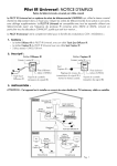
SIL Language Overview
The layers of SIL implementation are arranged in the following fashion:
Devices
Objects
Concurrency
Metaprogramming
Extended Types
Polymorphic Interactive Pascal
Figure 1-1
The SIL language
SIL Compared to Pascal
SIL and Pascal share many syntactic features. Programmers familiar
with Pascal, but new to SIL, can get started by treating SIL as an
interactive implementation of Pascal. SIL syntax is a superset of Pascal
syntax, and all of the control structures have their usual Pascal
meanings—basic data types such as reals, integers, booleans, and
records have standard behavior. The difference between the two
languages emerges when examining pointer types—SIL maintains
pointer structures in a Lisp or SmallTalk-like heap, so that pointer
management is different from (and simpler than) Pascal.
Still another feature which distinguishes SIL from Pascal is its
polymorphism. SIL is polymorphic in the sense that the same symbol
may be used to denote functions of differing input types. For example,
1-2
Soft Machines
the function double may be defined both for reals and points, without
conflict. This is known as static polymorphism (SIL supports other
kinds as well). Because the decision of which function variant to use is
made at compile time, no performance slowdown occurs.
The SIL Programming Environment
The SIL programming environment, like that of Lisp or SmallTalk, is
interactive. Any legal expression can be typed or cut and pasted into the
SIL> prompt, including new functions, type definitions, or global
assignments. Typing or pasting in expressions results in these new
entities being added to the current programming state. In Text Mode, the
mouse buttons have different functions (such as cutting and pasting
text), which are defined by the operating system.
Uncompiled SIL code is executed by a fast pseudo-code based
interpreter. It is possible to compile SIL code, also; to do this, the code
is translated first into C and then to binary using the host machine’s C
compiler. The performance of compiled SIL code is similar to that of
corresponding code written directly in C (or Pascal). Interpreted and
compiled code may be freely mixed—compiled functions may be
replaced at will by modified interpreted variants, allowing fast bug
fixing and testing.
The SIL Window can be used to enter SIL language commands while
retaining access to the menus and panels. The SIL Window is displayed
under the Graphics Window.
Figure 1-2
Developer’s Guide
(3/97)
The SIL Window
1-3
Introduction to the
SIL Language
SIL Language Overview
Introduction to the SIL Language
You can also change to Text Mode to enter SIL language commands. In
Text Mode, you have full editing capability and direct access to the
operating system.
Change to Text Mode by selecting Exit Menus from the File pulldown
menu. The menus are disabled and the SIL> prompt is displayed in the
shell window that you used to start Soft Machines.
Figure 1-3
Shell window example
Enter menus(); at the SIL> prompt to restore access to the menus. If the
system has become disabled, enter r(); at the Error> prompt to reset the
system.
The SIL Runtime Model
This section contains the following topics:
➢ Environments
➢ Values
➢ Expressions
■ Terms
■ Statements
■ Definitions
1-4
Soft Machines
SIL is an interpreted language. This means that an expression is read
from a file or the keyboard, and is passed to the SIL interpreter which
then computes the value of the expression. The computed value is
passed to a printer which writes it to a file or the screen, and the cycle
repeats.
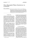
Figure 1-4 shows a representation of the relationships between the
components of the SIL runtime model.
Expressions
Reader
Values
Interpreter
Symbols &
Definitions
Printer
Values
Virtual
Memory
Figure 1-4
The SIL runtime model
Environments
Environments are either permanent or temporary. The permanent
environment is called the global environment. The global environment
contains bindings for
■ All type names
■ Function/procedure names
■ Global variables
Local environments contain bindings for
■ The parameters of a function/procedure
■ The local variables of a function/procedure
Developer’s Guide
(3/97)
1-5
Introduction to the
SIL Language
The SIL Runtime Model
Introduction to the SIL Language
Values
Values, or data objects, are the scalars and data structures such as
numbers, strings, records, and arrays that inhabit the computer’s
memory and represent abstract entities in the problem domain. The
generic term used in SIL to describe all of these objects is lispob (which
was derived from LISP OBject).
Lispobs may be classified into data types, or, to put it the other way
around, a data type can be viewed as a collection of similar lispobs.
Knowing the data type of a lispob is important. For example, this
information is used to compute the amount of memory space required to
store the lispob or to detect inconsistencies in a SIL program.
SIL data types fall into one of three broad categories:
■ System-defined types:
integer, real, boolean, string, …
■ Constructed types:
list types, array types, function types, …
■ User-defined types:
record types, classes, …
1-6
Soft Machines
Introduction to the
SIL Language
The SIL Runtime Model
Arrays
Lists
Constructed
Functions
Procedures
Types
Scalartypes
integer
real
boolean
string
Metatypes
ntype
Supertypes
lispob
universal
System-Defined
Records
User-Defined
Classes
Figure 1-5
Data type classifications
Expressions
NOTE
This section describes features in SIL which are identical
to Pascal, so you may want to skim, or even skip, this
section if you know Pascal.
There are three types of SIL expressions: terms, statements, and
definitions.
Developer’s Guide
(3/97)
1-7
Introduction to the SIL Language
Terms
There are three types of terms in SIL: constants, variables, and
function applications.
Example 1.2
constants:
variables:
applications:
2, -1.1, pi, "a_symbol, 'a string', nil, true, false
x, active_nc_machine, part_prog_name
sin(pi), max(2, x), mod(trunc(sin(x)), 50)
Other examples of function applications include infix operators,
which use the form:
<term> <operator> <term>
Other examples include special syntax for accessing fields of
records and components of arrays, as illustrated in Example 1.3.
Example 1.3
Infix operators:
Unary operators:
Array components:
Field selectors:
Mixed:
1-8
x + y, x / y, x and y, x > y, x = y
-x, not x
mount_point[x]
active_nc_machine.tlib
mount_point[x].holder
Soft Machines
Introduction to the
SIL Language
The SIL Runtime Model
Statements
Generally, a statement alters an environment. Statements can be
grouped into atomic statements and compound statements.
Atomic statements are assignment statements and procedure calls.
Example 1.4
Assignment statements:
x := y + 1;x := sin(y);tab[6] := 0.;
machine.tlib := lib_name;
Procedure calls:
writeln('hello', '....', 'world');
install(object_name, file_name);
Compound statements are built up from atomic statements using
statement constructors. There are three categories of statement
constructors: conditionals and case statements, sequences, and
iterations.
Sequences are groups of statements that are combined into a single
statement by bracketing them between the key words begin and end.
Conditional statements are in the form of IF statements (see
Example 1.5) or case statements (shown in Example 1.6)
Example 1.5
if x >= 0 then y := x;
if x >= 0 then y :=x else y := -x;
if test1 then
begin
if test 2 then
do_something()
else
do_nothing();
end
else
do_nothing();
Developer’s Guide
(3/97)
1-9
Introduction to the SIL Language
Example 1.6
Case s of
'!ABORT!': menu_return();
'!INIT!': init_nc_cell();
'SELECT MACHINE':
begin
select_nc_machine();
init_nc_cell();
end;
'SELECT TOOL LIB':
begin
select_nc_tool_lib();
init_nc_cell();
end;
'SIMULATE': call(ncv_simulation_imenu);
'MACHINE PENDANT': nc_machine_pendant();
'MODEL TOOLING': call(model_tooling_imenu);
'SAVE CELL SETUP': save_nc_setup();
'MISC': call(misc_functions_imenu);
end;
There are several types of iteration statements: repeat, while, and
for. The repeat and while statements behave similarly.
Example 1.7
A repeat statement can be used to check the validity of a user input:
{ Repeat reading string until end of file }
repeat
readln(fn, s);
ncv_batch_jobs_list := cons(s, ncv_batch_jobs_list);
end_of_file := eof(fn);
until end_of_file;
continued on next page
1-10
Soft Machines
Example 1.7
(continued)
An example of while:
{ While not end of file, read string and construct list }
while (not(eof(fn))) do
begin
readln(fn, s);
ncv_batch_jobs_list := cons(s, ncv_batch_jobs_list);
end;
An example of for:
for s in ncv_batch_jobs_list do
begin
writeln(fn, s);
end;
Definitions
SIL uses five categories of definitions:
• Global variable definition
• Variable declaration
• Type definition
• Procedure definition
• Function definition
Globals
The syntax for defining a new global variable or re-defining an
old global is
<variable> == <term>
Developer’s Guide
(3/97)
1-11
Introduction to the
SIL Language
The SIL Runtime Model
Introduction to the SIL Language
This statement assigns the value of <term> to <variable>, even if
<variable> was not previously declared or was assigned a value
of a different type.
Example 1.8
x == 22;
assigns the value 22 to the variable x.
x == 'hello world';
changes the value of x to the string hello world.
Types
To define new data types, use the following syntax:
type <type definition>; …; <type definition>;;
where
<type definition> ::= <type name> = <type>
In this case, <type> is a term which evaluates to a data type.
Notice the extra semicolon at the end of the declaration. This
tells the interpreter not to expect more type definitions.
Example 1.9
We can define several types in a single type definition:
type
years = integer;
dollars = real;
gcode_status =
lrecord
ok: boolean;
stmt_no: integer;
err_msg: string;
end;;
continued on next page
1-12
Soft Machines
Example 1.9
(continued)
type
gcode_closure =
tclosure(gcode_status, nc_machine,
gcode_info);
g_function =
lrecord
group: integer;
cl: gcode_closure;
end;
g_table = darray of g_function;;
Functions and Procedures
The format of function and procedure definitions follows Pascal
syntax (illustrated in Example 1.10).
Example 1.10
count == 0;
{ count is a global variable }
procedure inc_count();
begin
count := count + 1;
end;
procedure dec_count();
begin
count := count - 1;
end;
procedure reset_count();
begin
count := 0;
end;
procedure display_employee(e: employee);
begin
writeln(e.name);
writeln('salary = ', e.salary);
writeln('age = ', e.age);
end;
continued on next page
Developer’s Guide
(3/97)
1-13
Introduction to the
SIL Language
The SIL Runtime Model
Introduction to the SIL Language
Example 1.10
(continued)
procedure NCV_top_handler(s:string);
begin
case s of
'MOVE': do_mv();
'MODELING': do_md();
'LAYOUT WORKCELL': do_lw();
'INSTALL': do_in();
'SAVE': do_sv();
'DEVICES': call(xxcreate_models_imenu);
'MODELING': call(xxcreate_models_imenu);
'LAYOUT WORKCELL':
call(ncv_layout_workcell_imenu);
'NCV MENUS': call(ncv_module_imenu);
end;
end;
Example 1.11
function square(x: real): real;
begin
square := x * x;
end;
function average(x, y: real): real;
begin
average := (x+y)/2;
end;
function absolute_value(x: real): real;
begin
if x >=0 then
absolute_value := x
else
absolute_value := -x;
end;
continued on next page
1-14
Soft Machines
Example 1.11
(continued)
function distance(p1, p2: point);
begin
distance :=
sqrt(square(p2.xc - p1.xc) +
square(p2.yc - p1.yc) +
square(p2.zc - p1.zc));
end;
The primary difference between a procedure and a function is
that a function returns a value, whereas a procedure operates
purely by side effect.
Variable Declarations
The format of a variable declaration is
var <variable declarations>; …; <variable declarations>;;
where <variable declarations> is a list of variables followed by a
type expression:
<variable declarations> ::= <variable list> : <type>
Variable lists are variables separated by commas:
<variable list> ::= <variable>, …, <variable>
In the global environment, be sure to place a double semi-colon
at the end of the variable declaration so that the interpreter will
not expect more variable declarations.
Example 1.12
Several variables can be declared in a single declaration:
var
x,y,z: integer;
a,b,c: real;
i,j,k: darray of integer;
vmc: nc_machine;;
SIL will initialize integers to 0, reals to 0.0, and arrays to length 0
arrays. You should not, however, depend on this—you should
always initialize your own variables.
Developer’s Guide
(3/97)
1-15
Introduction to the
SIL Language
The SIL Runtime Model
Introduction to the SIL Language
Accessing Help
SIL includes a simple help facility:
help <name>;
The help command prints out all of the variants of the given name, their
types, and the name of the file in which they were defined.
Example 1.13 shows part of the information printed out for the plus
command in a Soft Machines state.
Example 1.13
SIL> help plus;
type = FUNCTION(INERTIA_MATRIX, INERTIA_MATRIX,
INERTIA_MATRIX) from file:
~/cim/builds/nbot_ops37/s/v_inertia.sil
protection: 0
type = FUNCTION(JV,JV,JV) from file:
~/cim/builds/nbot_typ26/s/v2mech2.sil
protection: 0
type = FUNCTION(JVR,JVR,JVR) from file:
~/cim/builds/nbot_typ26/s/v2mech2.sil
protection: 0
type = FUNCTION(AV,AV,AV) from file:
~/cim/builds/nbot_typ26/s/v6mech.sil
protection: 0
type = FUNCTION(GCOORD,GCOORD,GCOORD) from file:
~/cim/builds/device8/s/d2gcoord.sil
protection: 0
The help command also prints out type definitions.
1-16
Soft Machines
Chapter 2
Object-Oriented
Programming in SIL
Data Types
This chapter contains the following topics:
➢ Data Types
➢ Advanced Data Types
Object-Oriented
Programming in SIL
➢ C Data Types
➢ Casting
➢ Polymorphism
➢ Classes and Inheritance
➢ Concurrency
➢ Closures and tclosures
➢ Symbols
Data Types
This section contains these topics:
➢ Constructed Types
➢ System-Defined Types
➢ User-Defined Types
The SIL Type System uses the Pascal typing structure as a starting point
and expands on it. SIL provides types which are dynamically allocated,
and automatically collected from a heap. These types include dynamic
lists, arrays, strings, trees, and a special type, lispob.
All SIL data are of type lispob. lispobs can be partitioned into data
types, and data types can be classified as constructed, system-defined,
or user-defined types. This section describes the basic data types,
including lists, arrays, records, strings.
Developer’s Guide
(3/97)
2-1
Object-Oriented Programming in SIL
Types
Constructed
Arrays
Lists
System-Defined
Integers
Reals
Figure 2-1
NOTE
Strings
User-Defined
Booleans
Records
Classes
Basic SIL data types
The complete SIL data type structure is shown in Figure
1-5, “Data type classifications” on page 1-7.
Constructed Types
Constructed types are built from existing types using type constructors.
Some type constructors are list_of, array_of, function and procedure.
Lists
A dynamic list is a sequence of objects, all of the same type, which
can grow and shrink during program execution. You can define and
manipulate dynamic lists using the traditional Lisp operations: car,
cdr, and cons.
list_of(integer) is the type of all integer lists.
The base type of the type list_of(integer) is integer. Notice that
list_of(list_of(integer)) is another constructed type with base type
list_of(integer). list of integer is the alternative syntax for
list_of(integer).
The list operations ensure that the base type of a list is well-defined.
For example, the call
list(1, 2, 'hello world')
2-2
Soft Machines
results in a type mismatch error, since all of the arguments are not of
the same type. This seems fairly straightforward until we consider
empty lists (lists with 0 members). What is the base type of an
empty list? To solve this problem in SIL, you need to declare the
base type whenever you create an empty list. A call to the empty list
constructor has the form
emptylist(<type>)
where <type> is any type expression and indicates the base type of
the empty list returned by this call. Of course, you must be able to
determine whether or not a list is empty. To check whether or not a
list is empty, use the predicate
null(<list>)
which returns TRUE if <list> is an empty list (of any base type).
Arrays
array_of(integer) is the type of all arrays of integers (regardless of
size).
The base type in this case is integer. darray of integer is the
alternative syntax for array_of(integer). Like lists, SIL arrays are
also dynamic. This means that arrays can be created during program
execution. The call
array_create(<type>, <integer>)
returns an array of base type <type> indexed from 0 to <integer>. As
in Pascal, if v is an array and i is a valid index, then v[i] is an
expression whose value is the element of v with index i, and v[i] :=
<term> sets the index i component of v to be the value of <term>. As
with lists, the type of <term> must match the base type of v, or a type
mismatch error will result.
Unlike Pascal, SIL functions can return arrays as values.
Developer’s Guide
(3/97)
2-3
Object-Oriented
Programming in SIL
Data Types
Object-Oriented Programming in SIL
sarrays
An sarray is a dynamically-allocated array, which can grow and
shrink during program execution. You can add items to the sarray,
and the sarray will automatically resize itself to fit the new
elements. As with standard arrays, if s is an sarray and i is a valid
index then s[i] returns the ith element of the sarray, and s[i] :=
<term> sets the index i component of s to be the value of <term>.
Also, like arrays, <term> must match the base type of s, or a type
mismatch error will occur.
The command
emptysarray(<type>)
returns a new sarray.
Functions and Procedures
■ function(real, integer, integer) is the type of all functions
that take two integer inputs and return a real output. Integer
division is a function in this type.
■ procedure(real, integer) is the type of all procedures which
expect a real-valued and integer-valued input.
System-Defined Types
SIL system-defined types include the basic scalar types: integer, real,
boolean, string.
Strings
Strings are dynamic in SIL.
Example 2.1
The definition:
msg == 'hello';
assigns the length 5 string hello to the variable msg. Later, we can
reassign msg’s value by:
msg := 'goodbye';
2-4
Soft Machines
Data Types
msg := 'bye';
String Comparisons
In SIL, users make lexicographical comparisons using the syntax
<string> < <string>
Additionally, we can compare strings using: <=, >, >=, =, and <>.
The match operator compares strings that may contain wildcards.
String Conversions
A string composed of numerals can be converted to an integer by
using
string_to_integer(<string>)
Conversely, an integer can be converted to a string by using
integer_to_string(<integer>)
Similarly, we can convert reals to strings and back with
real_to_string(<real>)
and
string_to_real(<string>)
lstrings
Consider the following assignments:
x := 'abcdffg';
x := substring(x,2,3);
Developer’s Guide
(3/97)
2-5
Object-Oriented
Programming in SIL
In the above example, we assign a length 7 string (goodbye) to the
same variable. Memory allocation for the additional characters is
handled automatically. Of course shorter strings can be assigned to
msg:
Object-Oriented Programming in SIL
These assignments result in the value of x being 'bcd'. The SIL
interpreter will construct a new three-character string for the second
assignment. Repeated assignments like these can result in an
inefficient consumption of memory. To combat this problem, SIL
provides an lstring, which can be defined as follows:
lstring = lrecord
length: integer;
contents: string;
end;;
Primitive operations on lstrings:
function mk_lstring(x: string): lstring;
function mk_lstring(x: string; n: integer): lstring;
function copy(x: lstring): lstring; { Allocates a new string }
function substring(x: lstring; n,m: integer): lstring;
function select(x: lstring; n,m: integer): lstring;
function equal(x: lstring; y: string): boolean;
function select(x: lstring; y: integer);
procedure lowercase(x: lstring);
procedure concat_onto(y: string; x: lstring);
function lstr_to_str(x: lstring): string;
function to_lstring(x: string): lstring;
procedure float2lstr(y: real; ls: lstring);
function find(cnx: string; lnx: integer; cny: string;
lny: integer): integer;
function find(x: string; y: string): integer;
function find(x: lstring; y: string): integer;
function find(x: lstring; y: lstring): integer;
procedure concat_onto(x: lstring; n: char);
User-Defined Types
User-defined types are created by type definitions:
type <name> = <type expression>;;
Any kind of type expression can be used in a type definition.
Two of the most commonly-used of these types, records and lrecords,
are described in the following sections.
2-6
Soft Machines
Data Types
Records
Records are always defined within the scope of a type definition at
the top level. The syntax follows Pascal:
Object-Oriented
Programming in SIL
type
<name> = record
<field>, … <field>: <type>;
…
<field>, … <field>: <type>;
end;;
where <field> and <name> are identifiers.
Unlike Pascal records, defining a record in SIL automatically
defines a constructor function which enables you to create records
in a single statement. The name of the constructor function adds the
prefix mk_ to the name of the record.
Unlike Pascal, SIL functions can return records as values.
lrecords
Record parameters are passed by value. This means that a
function/procedure which is passed a record as an input actually
makes a private copy of the record input before it modifies any of
its fields.
In SIL, records are used to represent non-mutable entities and
lrecords are used to represent mutable structures. An lrecord is just
a pointer to a record—lrecord parameters are passed by reference
rather than by value. This means that a function/procedure only gets
a pointer to an lrecord, not a private copy.
Developer’s Guide
(3/97)
2-7
Object-Oriented Programming in SIL
Advanced Data Types
This section contains these topics:
➢ ntype
➢ Supertypes
➢ Applications
SIL system-defined types include the basic scalar types: integer, real,
boolean, string. But SIL also provides some fairly exotic types. For
example, internal representations of SIL expressions and their
components are also ordinary SIL data objects which can be
manipulated by SIL programs the same way that scalars can. These are
called metaobjects, and the types to which they belong are called
metatypes.
Another category of useful system-defined types is the supertypes. If
we think of types as sets of values, then all types can be regarded as
subsets of the supertypes. The two supertypes are lispob and universal.
System-Defined
Types
Scalartypes
string
integer
boolean
Figure 2-2
2-8
Metatypes
real
ntype
Supertypes
lispob
universal
System-defined type classifications
Soft Machines
Advanced Data Types
ntype
<ntype> ::= <dtype> | <polymorphic type>
<dtype> ::= <primitive type> | <constructed type>
<primitive type> ::= <user defined type> | <atomic type>
<atomic type> ::= <scalar type> | <metatype> | <supertype>
<scalar type> ::= integer | boolean | char | string | real
<metatype> ::= id | sconst | ntype | tform | iform | net | event | …
<supertype> ::= universal | lispob
<constructed type> ::= array_of(<dtype>) | list_of(<dtype>)
| sarray_of(<dtype>)
| closure(<return type>,<input type>,...,<input type>)
| tclosure(<return type>,<input type>,...,<input type>)
<polymorphic type> ::= function(<return type>,<input
type>,...,<input type>)
| procedure(<input type>,...,<input type>)
| task(<return type>,<input type>,...,<input type>)
<input type> ::= <dtype>
<return type> ::= <dtype>
Notice that ntype appears to be a member of itself. However, it is really
the syntactic expression ntype that is a member of the data type ntype,
so Russell’s paradox is avoided.
Developer’s Guide
(3/97)
2-9
Object-Oriented
Programming in SIL
The type ntype, the “type of all types”, can be defined grammatically by
Object-Oriented Programming in SIL
The following is a partial list of the primitive operations on ntype. The
names of the functions are self-documenting:
function is_primitive (n:ntype):boolean;
function is_reptyp (n:ntype):boolean;
function is_array (n:ntype):boolean;
function is_list (n:ntype):boolean;
function rep_of(n:ntype):ntype; { assumes n is represented type }
function list_subtype(x:ntype):ntype;
function subtype(x:ntype):ntype;
function subtypes(x:ntype):list_of_ntype;
function mk_list_type(x:ntype): ntype;
function mk_array_type(x:ntype): ntype;
function is_function (n:ntype):boolean;
Assume x = result type, y = input types:
function mk_function_type(x:ntype;y:list_of_ntype): ntype;
{ assumes a real function type is the input: }
function is_task(x:sconst):boolean;
function is_closure(x:sconst):boolean;
function is_tclosure(x:sconst):boolean;
function input_types(x:ntype):list_of_ntype;
function result_type(x:ntype):ntype;
2-10
Soft Machines
Advanced Data Types
SIL supertypes include lispob and universal. Supertypes are ordinary
data types; they can appear in type definitions, variable declarations, and
as input or output types for functions. What makes supertypes “super”
is that SIL data objects of any type can be legally cast to a supertype
using SIL’s as_type operation.
Example 2.2
3 as_type lispob;
2.7 as_type lispob;
'Good Morning' as_type lispob;
list(1,2,3,4) as_type lispob;
3 as_type universal;
2.7 as_type universal;
'Good Morning' as_type universal;
list(1,2,3,4) as_type universal;
lispobs
The type lispob is the SIL type whose values include all SIL values
(lispob was derived from LISP OBject). ob is short for lispob, i.e.,
ob == lispob. Example 2.3 illustrates how to use ob to resolve SIL
typing restrictions.
Example 2.3
Suppose we want to write a function to check whether two lists of
integer is identical:
function same_list(l1, l2: list of integer): boolean;
begin
if (l1 = l2)
then same_list := true
else
same_list := false;
end;
continued on next page
Developer’s Guide
(3/97)
2-11
Object-Oriented
Programming in SIL
Supertypes
Object-Oriented Programming in SIL
Example 2.3
(continued)
We will get the error message:
type mismatch in application of the
operator EQUAL
This can be resolved by casting the variables l1 and l2 into obs
before applying the equal operator:
function same_list(l1, l2: list of integer): boolean;
begin
if ((l1 as_type ob) = (l2 as_type ob))
then same_list := true
else
same_list := false;
end;
The same function can be written as
function same_list(l1, l2: list of integer): boolean;
begin
same_list := ((l1 as_type ob) = (l2 as_type ob));
end;
Test cases:
SIL> same_list(list(1,2,3,4), list(1,2,3,4));
TRUE
SIL> same_list(list(1,2,3,4), list(1,2,3,4,5));
FALSE
We can create an even more general version of this function by using
obs as input arguments:
function same_list(l1, l2: list of ob): boolean;
begin
same_list := ((l1 as_type ob) = (l2 as_type ob));
end;
Test cases:
SIL> same_list(list(1 as_type ob, 2 as_type ob),
list(1 as_type ob, 2 as_type ob));
TRUE
continued on next page
2-12
Soft Machines
Advanced Data Types
Example 2.3
(continued)
SIL> same_list(list('a' as_type ob, 'Good Morning' as_type ob),
list(1 as_type ob, 2 as_type ob));
SIL> same_list(list('a' as_type ob, 'Good Morning' as_type ob),
list('a' as_type ob, 'Good Morning' as_type ob));
TRUE
SIL> same_list(list('a' as_type ob, mk_point(10.,20.,30.) as_type
ob),
list('a' as_type ob, mk_point(10.,20.,30.)
as_type ob));
TRUE
universals
All SIL data tagged by type is type universal. As with lispob, any
SIL expression can be cast to universal and back. A universal is a
type tagged lispob implemented as a SIL type:
type universal = lrecord
value_of: lispob;
type_of: ntype;
end;;
Like any other records, universals can be constructed either by using
the automatically-defined constructor: mk_universal or by using
as_type. universal is most useful if you need to figure out the type
of a SIL data object, as illustrated in Example 2.4.
Example 2.4
Checking types of SIL variables:
SIL> type_of(2 as_type universal);
INTEGER
SIL> type_of('Good Morning' as_type universal);
S_T_R
continued on next page
Developer’s Guide
(3/97)
2-13
Object-Oriented
Programming in SIL
FALSE
Object-Oriented Programming in SIL
Example 2.4
(continued)
SIL> type_of(pi as_type universal);
RANGLE
SIL> type_of(mk_point(10.,20.,30.) as_type universal);
POINT
SIL> type_of(pose('teacher') as_type universal);
FRAME
SIL> type_of(wlkup('teacher') as_type universal);
SHAPE
Example 2.5 shows how to store and retrieve data of different types
using universals.
Example 2.5
A common requirement for a tooling database is to store tool offsets
(length, radius, etc.) with a tool library. The format of this data,
however, may vary with the type of machine-tool (lathe versus
machining center) and with the controller used. We can store and
retrieve this data using the same SIL type definition by using
universal.
The SIL declaration for the class tool_lib (tool library) is as follows:
new_class(tool_lib,
superclass: generalize: shape,
changer: tool_changer,
aux: universal);
The class tool_lib is a subclass of shape, which describes the
geometry of the tool library in a workcell. The field changer (of type
tool_changer) contains data for the tool changer associated with the
tool library, and the aux (auxiliary field, of type universal) contains
the tooling data.
NOTE A more detailed description of classes will be described in “Classes
and Inheritance” on page 2-24. See Chapter 4, “Geometry in
Soft Machines” for shape and geometry.
continued on next page
2-14
Soft Machines
Advanced Data Types
(continued)
The aux field gives us the flexibility of attaching tooling data of
different formats to the tool library. For example, the tooling data for a
vertical machining center “vmc” is contained in an array of type
vmc_tdata. We can retrieve the tooling data from the variable
vmc_tlib (type tool_lib) as follows:
var atod: darray of vmc_tdata;;
if (type_of(vmc_tlib.aux) = type_of(atod)) then
atod := vmc_tlib.aux as_type darray of vmc_tdata
else
writeln('Tool lib contains the wrong data type');
Note that we can first validate that the field vmc_tlib.aux contains the
correct data type before we cast the tooling data from universal to
vmc_tdata.
Applying Procedures
To write a dispatch procedure using universals, we need to use the
apply operator to apply the appropriate assemble procedure.
function apply(op: id; arg1, arg2, … :): universal
where op is the name of an operator, and arg1, arg2, … are the
arguments to op.
APPLY: type = FUNCTION(LISPOB,LISPOB,LISPOB) from file:
<NULL S_T_R> protection: 0
APPLY: type = FUNCTION(LISPOB,LISPOB,LIST(LISPOB)) from
file: <NULL S_T_R> protection: 0
type = FUNCTION(AN_IFORM,ID,LIST(IFORM)) from file: <NULL
S_T_R> protection: 0
APPLY: type = FUNCTION(LISPOB,ID,LIST(LISPOB)) from file:
<NULL S_T_R> protection: 0
type = FUNCTION(LISPOB,SCONST,LIST(LISPOB)) from file:
~/cim/builds/nevent51/s/e5_4ap.sil protection: 0
type = FUNCTION(UNIVERSAL,ID,LIST(UNIVERSAL)) from file:
~/cim/builds/danal194/s/a_6univ2.sil protection: 0
type = FUNCTION(UNIVERSAL,APPLICATION,LISPOB) from file:
~/cim/builds/danal194/s/a2_2app.sil protection: 0
Developer’s Guide
(3/97)
2-15
Object-Oriented
Programming in SIL
Example 2.5
Object-Oriented Programming in SIL
The apply operator provides what is called late binding. Late
binding means that the decision as to which variant of a function is
designated by a function name is made at the latest possible moment:
when the function application is actually being executed. Ordinary
function application in SIL is of the early binding style: the
selection of variant is made at the earliest possible time—when the
code is read in.
We are now ready to write dispatch:
procedure dispatch(part: universal);
begin
apply("assemble, part)
end
A call to dispatch would look like
dispatch(part as_type universal);
The applyn operator works in a similar fashion, but it returns a
failure indicator when no variant is found. The function is_fail
determines whether or not a universal value indicates failure.
Applications
Applications are entities that remember a function and a list of
arguments. They are similar to closures, with the added feature of an
argument list that can be stored and passed to the function when the
application is executed. This function constructs an application:
function mk_application(fn : id; args : list of universal) :
application;
An application contains the identification (id) of a function and the
arguments to be passed to it when executed.
This function executes an application:
function execute(app: application):universal;
The application function is called with the included arguments.
2-16
Soft Machines
C Data Types
C Data Types
Object-Oriented
Programming in SIL
This section contains these topics:
➢ C Records and C Arrays
➢ C Strings
➢ C Constants at Build Time
C Records and C Arrays
Any SIL record or lrecord includes a tag word at the beginning for use
by the garbage collector. Any SIL array or string has such a tag word
too, as well as a length field. The crecord facility in SIL allows records
and arrays to be declared without including these additional tag words
and length fields. The main motivation for this is to allow direct
manipulation by SIL code of any C data structure.
The syntax of a crecord declaration is just like that of a record or
lrecord:
type erb = crecord
xc: integer;
yc: real;
end;;
This is identical in effect to the C declaration:
struct erb { int xc; double yc; };
then
new(erb);
returns a value of type
^erb
i.e., pointer to erb, which is equivalent to the C type *erb.
Developer’s Guide
(3/97)
2-17
Object-Oriented Programming in SIL
The usual SIL syntax can be used to select and set the fields of an erb:
ee == new(erb); ee . xc := 56; ee .yc := 5.4 + ee . xc;
Similarly, a carray is an array without tag or length fields. A carray can
be created with
cc == carray_create(integer,10);
The “^” syntax can be used to make a pointer, as in
aa == ^(ee . xc);
or
aa == ^cc[4];
The type of aa is ^integer. The only legal arguments to ^ are fields of
crecords and entries in carrays. Pointers are de-referenced as follows:
aa^;
then
aa^ := aa^ + aa^;
will double the integer value pointed to by aa.
crecords and carrays can be built from the primitive types cchar,
cshort, integer, real, sreal or from other crecords or carrays.
SIL Type
Identical to C Type
cchar
char
cshort
short
sreal
float (single precision real)
integer
int
real
double
The types cchar, cshort, and sreal should appear only as the subtypes
of carrays, pointers, or crecords.
2-18
Soft Machines
C Data Types
Alignment is done as in C—each type is aligned to an even multiple of
its length.
cchars and cshorts when extracted turn into SIL integers, and sreals
C Strings
There are a couple of utilities for going back and forth between SIL
lstrings and C strings.
The type cstring is defined just to be a synonym for carray_of(cchar).
The following operations are provided:
function to_cstring(x: lstring): cstring;
This first checks that the contents string of x is static (does not get
moved around by the garbage collector) and null-terminated. If either of
these conditions is violated, a new contents which is tenured and
null-terminated is generated and set up as the contents part of x. The
cstring returned is a pointer to the “raw” (untagged) contents of x. So,
the cstring will occupy the same storage as the contents of x, and will
be null-terminated. Since the storage for the resulting cstring cannot be
freed, this function should be used only to create permanent cstrings.
The following function statically allocates a brand-new null-terminated
cstring with capacity equal to that of x, and copies x into it. Since the
storage for the resulting cstring cannot be freed, this function should be
used only to create permanent cstrings.
function mk_cstring(x: lstring): cstring;
REMINDER
The capacity of an lstring is usually bigger than its
current length.
The following function dynamically allocates a brand-new nullterminated cstring with capacity equal to that of x, and copies x into it.
The storage for the resulting cstring can be freed with free_cstring.
function new_cstring(x: lstring); cstring;
Developer’s Guide
(3/97)
2-19
Object-Oriented
Programming in SIL
into SIL reals.
Object-Oriented Programming in SIL
This procedure frees the x cstring, which has been created dynamically
by new_cstring:
procedure free_cstring(x: cstring);
This procedure copies c to x, stopping at a null in c, or the capacity of x,
whichever comes first:
procedure copyto(x: lstring;c: cstring);
The following procedure copies x into c. Since c has no length
indication, this can be dangerous—if c was allocated to be shorter than
the current length of x, then the memory after c’s length allocation will
be deleted.
procedure copyto(c: cstring;x: lstring);
The print function for cstrings will print characters until a null is hit, or
the limit max_cstring_print_length is reached.
max_cstring_print_length is initially 100.
If you want to allocate an lstring to be passed to C, you may wish to use
function mk_static_lstring(x: string;n: integer): lstring;
or
function mk_static_lstring(x: string): lstring;
Either of the above functions are used to construct lstrings that are
already static and null terminated.
This procedure will cause the contents of x to become static and null
terminated (if they are not already):
procedure mk_static(x: lstring);
2-20
Soft Machines
Casting
C Constants at Build Time
“Builds” are described in Chapter 3, “Working with
SIL Code”.
C data structures can only be safely created at build time by using the
construct
cstring_constant(aa,'abc');
This has exactly the same effect as
aa == mk_cstring('abc');
except that cstring_constant records the need to reset aa when a state
starts up, making it safe for use in compiled code.
Casting
In SIL, an expression’s type can be modified by the as_type operator.
The effect of this operator is analogous to that of the C cast primitive—
it asserts that the value of the expression should be treated as belonging
to a specified type, whatever the type originally assigned to the
expression may have been. The syntax is
<expression> as_type <type>
Example 2.6
SIL> var d1, d2: dangle;; { “dangle” is angle in deg }
The SIL expression
SIL> d1 := 30.;
will give the following error message:
error: COULD NOT COERCE REAL TO DANGLE IN 30.00000
This is because SIL regards dangle and real as distinct data types.
continued on next page
Developer’s Guide
(3/97)
2-21
Object-Oriented
Programming in SIL
NOTE
Object-Oriented Programming in SIL
Example 2.6
(continued)
A solution would be to cast 30. to type dangle with the following
expressions:
SIL> d1 := 30. as_type dangle;
To continue with our example:
SIL>
SIL>
SIL>
SIL>
d2 := d1 + pi/4.;
var r1: real;;
r1 := d2 as_type real;
r1;
75.0000000
Not all as_types are legal. The rule (which has a few exceptions given
later) is that the data format of the value to be cast must agree with the
data format of the type to which it is being cast. Another restriction is
that a record cannot be cast to an lrecord, nor an lrecord to a record.
SIL Constants
All SIL definitions have internal representations called sconsts (SIL
constants). An sconst is like a descriptor which contains type, name,
and value fields for the defined object.
Because SIL is a polymorphic language, a single id x can be the name of
several sconsts. However, only one of these sconsts can represent a
non-function type. This sconst is the data variant of x; the other sconsts
are the function variants of x. The following operators help locate an
sconst using an id:
function data_variant(x:id): sconst;
function has_data_variant(x:id): boolean;
function function_variants(x:id): list of sconst;
function has_function_variant(x:id): boolean;
2-22
Soft Machines
Polymorphism
function find_variant(x: id; intps: list of ntype): sconst;
More generally, an id and a type specify an sconst which can be fetched
by
function find_variant(x: id; tp: ntype): sconst;
If there is no variant of the indicated type, a special sconst,
undefined_sconst is returned. To test for undefined_sconst:
function is_undefined(x: sconst): boolean;
This function applies the given sconst to the given arguments.
apply(op: sconst; a: list of lispob);
Polymorphism
A polymorphic typing system is one which permits one name to name
several objects at the same time as long as these objects have different
types. For example, the function sin accepts both rangle and real type
inputs. In SIL, a name can have at most one data variant but any number
of function variants. Each function variant, however, must have distinct
input types (for instance, moveto in SIL has over 20 variants).
Consequently, in Example 2.7, these two variants of same_list can
coexist at the same time.
Example 2.7
function same_list(l1, l2: list of integer): boolean;
function same_list(l1, l2: list of ob): boolean;
Developer’s Guide
(3/97)
2-23
Object-Oriented
Programming in SIL
Because two function variants with the same name must have distinct
input types, a name and a list of input types uniquely specify an sconst
for a function variant. We can fetch this sconst with
Object-Oriented Programming in SIL
Classes and Inheritance
This section contains these topics:
➢ Classes
➢ Inheritance
➢ Specialization and Generalization (how objects are viewed
relative to each other, and how to manipulate the views)
➢ Abstract Classes
One of the main characteristics of object-oriented programming is the
concept of inheritance. Two objects, A and B, belonging to different
types (classes), can be related in such a way that all properties of A are
also properties of B. In this case, B inherits A’s properties. In SIL
terminology, B is a specialization of A, since B may have additional
“specialized” properties apart from those inherited from A; or A is a
generalization of B. Applying this concept to machine-tools, we can say
that a machining center is a specialization of an NC machine, which in
turn is a specialization of a kinematics device.
The advantage of inheritance is that programmers do not have to build
an object from the ground up. By declaring object B to be a
specialization of A, the properties of A automatically become properties
of B. This is especially useful if A is a system-defined object with many
useful, but low-level, properties. For example, B might be a cutting-tool
with properties such as location of cutting tip, cutting edge, etc., whereas
A might be a CAD model with geometric and graphical properties such
as boundary representation, surface normals, color, etc. If you are
creating a simulation of an NC machining process, you are probably
familiar with the cutting properties of a cutting-tool, but may not be
familiar with the lower level properties of a CAD model, even though
these properties are necessary for displaying and manipulating the
cutting-tool in a simulation. Because Soft Machines provides a type
(class) shape, which represents a simulated object in three-dimensional
space, the class cutting_tool (cutting tool) can simply be described as a
specialization of shape.
2-24
Soft Machines
Classes and Inheritance
Classes
The definition of a class in SIL is very similar to a Pascal (or SIL) record
definition:
Object-Oriented
Programming in SIL
type <new_class> = class
superclass:<class1>;
superclass:<class2>;
…
<instance-var-1>:<type1>;
<instance-var-2>:<type2>;
…
end;;
Example 2.8 illustrates how to define a subclass for a cutting tool.
Example 2.8
new_class(cutting_tool,
superclass: generalize: shape,
flange: frame,
{ Mount flange }
tip: frame,
{ Cutting tip }
cutter_type: id,
{ Cutter characteristics }
diam: real,
length: real,
cutting_angle: rangle,
flute_length: real);;
To model a cutting tool, follow this sequence:
1. Construct a Soft Machines model using the CAD Interfaces panel
or the Modeling pulldown menu.
2. Teach flange and cutter tip on model.
3. Declare other cutter characteristics.
4. Construct cutting tool using
mk_cutting_tool(wlkup(<model_name>), cutter_flange,
cutter_tip, .... );
Developer’s Guide
(3/97)
2-25
Object-Oriented Programming in SIL
Inheritance
Class inheritance is used extensively throughout Soft Machines. As
mentioned earlier, a machining center is a specialization of an NC
machine, which is a specialization of a robot. Thus, the class
nc_machine inherits all the properties of the class robot, such as
forward and inverse kinematics, joint limits, velocity and acceleration,
etc. In other words, all functions using robot as input type can also be
used for nc_machine, without explicit casting to type robot.
Example 2.9 introduces the principles of inheritance. In this example,
robot-related functions are used for NC machines.
Example 2.9
Suppose the variable vmc is of type nc_machine, a subclass of robot.
We can use robot-related functions on vmc, such as
Current joint vector of vmc:
c_jv(vmc);
Move axes (links) of vmc:
moveto(vmc, c_jv(vmc)+mk_jv(10.,20.,0.,0.,0.,0.));
Move one link (Link 1) by 10cm.
moveby(wlkup(vmc), 1, 10.);
2-26
Soft Machines
Classes and Inheritance
Specialization and Generalization
Figure 2-3 shows a simplified class hierarchy of objects in
Soft Machines. All geometric entities in a Soft Machines workcell
are represented as type shape.
shape
device
end effector
cutting_tool
tool_holder
tool_changer
tool_library
robot
nc machine
machining
center
Figure 2-3
Object class hierarchy
The specialize_to operator is used to access subclasses of any
Soft Machines object. Conversely, to access the superclass of an
object, generalize is used. When an object is first installed into a
workcell (as type shape), we use specialize_to to retrieve the
subclass. We can also determine whether a shape contains the valid
subclass by checking whether specialize_to returns a nul.
Example 2.10
Install cutting tool from file:
var sh: shape;
ct: cutting_tool;;
sh := install(<shape_name>, <file_name>);
ct := specialize_to(sh, cutting_tool);
Developer’s Guide
(3/97)
2-27
Object-Oriented
Programming in SIL
The specialize_to Operator
Object-Oriented Programming in SIL
Example 2.10
(continued)
Check whether a shape contains an NC machine:
function is_nc_machine(sh: shape): boolean;
begin
if object_exists(name(sh)) then
is_nc_machine :=
not(nul(specialize_to(sh, nc_machine)))
else
is_nc_machine := false;
end;
Views
Two objects are referentially equivalent if they are both views of
the same entity. Clearly, if object A generalizes object B, then A and
B are referentially equivalent. But two objects can be referentially
equivalent without one generalizing the other.
The list of all views referentially equivalent to an object is given by
the function views. The views function returns a list of universals
(objects, like any other SIL data, can be cast to and from universals).
The list of classes to which these views belong is given by the
function classes. This is a list of ntypes. The class of an object is
given by the function my_class.
Because referentially equivalent objects represent the same entity,
we would like all views of A (i.e., not just the specializations of A),
to be able to use the methods and attributes of A. Doing this requires
changing views using the as_view or to_view infix operator:
<object> as_view <class>
<object> to_view <class>
When <object> has no view in <class>, <object> as_view <class>
generates an error message while <object> to_view <class> returns a
null object which can be tested for using the nul predicate.
Two simple operators are provided for directly manipulating the
views of an object: splice and remove_this_view.
2-28
Soft Machines
Classes and Inheritance
The splice operator works like this:
splice(<object1>,<object2>);
The remove_this_view operator works like this:
remove_this_view(<object>);
The remove_this_view operator will generate an error if the class of
any other view of the object is a subclass of the class of the view
being removed. If this restriction were not observed, objects with
dangling superclass pointers would result.
A view which has been removed should not be referenced after its
removal.
Abstract Classes
This section describes the abstract class facility and is intended for
advanced SIL language users. This section includes the following
topics:
■ Installation of Methods
■ Additional Methods Primitives
■ The mnode Class
The abstract class facility provides the same sort of functionality as C++
virtual functions—you can define abstract classes whose methods can
be implemented by a variety of concrete classes. The facility is more
flexible than anything available in C++ in that it allows dynamic
modification of the implementing classes and methods of an abstract
class. Abstract classes can also be spliced onto pre-existing concrete
classes, allowing abstractions to be layered onto existing bodies of
concrete code.
Developer’s Guide
(3/97)
2-29
Object-Oriented
Programming in SIL
The splice operator simply appends the views of object1 onto those
of object2. So, object1 and object2 are unified—they become
referentially equivalent. object1 may not be spliced onto object2 if
any view of object1 has the same class as a view of object2.
Object-Oriented Programming in SIL
Example 2.11 introduces abstract classes by showing a conventional
example—an “abstract stack” class.
Example 2.11
type astack = class
push: method(ob,ob);
ipop: method(ob);
empty: method(boolean);
on_underflow: method(ob);
end;;
NOTE
This example will be continued after the following information.
The method fields are slots which hold operators on astack, just as
ordinary fields of a class hold data. The usage
method(<return-type>,<input_type1>,… <input_typen>)
specifies a “method” which can be applied to inputs of types astack,
<input_type1> ...<input_typen>, and will return the given return type.
So, for example, push takes an astack and an ob, and returns an ob. The
first argument to any method is the class for which the method is
defined, so it need not be specified explicitly. It is for this reason that we
write method(ob,ob) rather than the redundant method(ob,astack,ob).
Now, the method slots in a class definition are filled by ordinary SIL
functions which take a view of the astack as first argument. For
example, the operator installed in the push slot will be a procedure
which takes a view of an astack as its first argument, and an ob as its
second. The intent of this should become clear as we proceed with this
example.
Example 2.11
(continued from above)
Now, we define the concrete class lstack:
type lstack = class
superclass:astack;
goods:list of ob;
end;;
2-30
Soft Machines
Classes and Inheritance
Example 2.11
(continued from above)
Object-Oriented
Programming in SIL
Here are some of its methods:
procedure push(x:lstack;y:ob);
begin
x . goods := cons(y,x . goods);
end;
function pop(x:lstack):ob;
begin
if null(goods(x)) then pop := nil else
begin
pop := car(goods(x));
x .goods := cdr(goods(x));
end;
end;
function empty(x:lstack):boolean;
begin
empty := null(goods(x));
end;
Installation of Methods
Installation of methods is done using the following primitives. If a is a
particular astack, which is also an lstack, we can set the method push
in a to be push on the lstack. The following does this:
a == mk_astack();
l == mk_lstack(a,emptylist(ob));
set_method(a,"push,"push,list(lstack,ob));
That is, when push is called on a, it “delegates” the work to the push
variant on lstack. So,
push(a,x);
is equivalent in effect to
push(a as_view lstack,x);
Developer’s Guide
(3/97)
2-31
Object-Oriented Programming in SIL
Example 2.12
a == mk_astack();
l == mk_lstack(a,emptylist(ob));
set_method(a,"push,"push,list(lstack,ob));
function pop(x:astack):ob;
begin
if empty(x) then
begin
if method_defined(x,"on_underflow) then
on_underflow(x);
pop := nil;
end
else
pop := ipop(x);
end;
As illustrated above, the operator
method_defined(x:<any type>;y:id);
determines whether the given method has been installed in x.
The following operator makes an astack with the lstack
implementation:
function mk_lstack(): astack;
var a: astack; l: lstack;
begin
a := mk_astack();
l := mk_lstack(a,emptylist(ob));
set_method(a,"push,"push,list(lstack,ob));
set_method(a,"ipop,"pop,list(lstack));
set_method(a,"empty,"empty,list(lstack));
mk_lstack := a;
end;
Note that no method is assigned to on_underflow. A user of astack is
free at any time to execute a set_method to install a method for
underflow.
2-32
Soft Machines
Classes and Inheritance
Additional Methods Primitives
The following are more primitives for methods.
prints out the methods currently installed in x. This is useful for
debugging.
define_method(astack,lstack,"ipop,"pop);
Instead of installing a method into any particular astack, the above use
of define_method defines a standard method to use for ipop for any
object that is an astack implemented by an lstack. For astack a
use_methods(a,lstack);
installs all of the standard methods for astack associated with lstack
into a.
The pop method does not get installed by define_methods because ipop
is the abstract method name, while pop is the implementation name.
Rule 2.1
To remember the argument order for the above primitives, an easy rule is
Abstract information always precedes the concrete information in
the argument order.
Methods can be declared to be tasks rather than procedures by using the
keyword tmethod rather than method.
The mnode Class
mnode is an abstract class, and is the class of all screen items (widgets).
The word mnode comes from “node in the menu tree.” Actual widgets
are built by subclassing and/or splicing an mnode.
Developer’s Guide
(3/97)
2-33
Object-Oriented
Programming in SIL
pmethods(x:<any_type>);
Object-Oriented Programming in SIL
Concurrency
This section explains how to use SIL for concurrent execution of
multiple tasks within one “state” or data space. This section contains
these topics:
➢
➢
➢
➢
➢
Tasks
Tickers
Semaphores
Pipes
Processes
SIL maintains a global variable called clock which measures the passing
of simulated time. Certain SIL commands cause clock to be advanced
when they are called. Commands that consume simulated time are called
temporal. Non-temporal commands are called instantaneous. A block
of instantaneous commands is called an instantaneous block.
Temporal commands are used in simulations that model time. These
commands include those that move or operate kinematics devices such
as robots, NC machines, and automatic tool changers.
Do not confuse simulated time with real time. An infinite loop will
consume an indefinite amount of real time, but may consume no
simulated time if it contains only instantaneous commands. Simulated
time is also independent of the computer hardware used or system load,
and is determined by the task scheduler based on the kinematics
characteristics (distance moved, velocity, acceleration, etc.) of the
simulated object. A simulation running on a faster computer may
consume less real time, but the simulated time should be identical if the
same simulation is run on a slower computer.
2-34
Soft Machines
Concurrency
All SIL function and procedure calls are instantaneous. No temporal
commands can be called in the body of a function of procedure.
Temporal commands are created by defining tasks. The syntax for
defining a task is similar to that for defining functions and procedures
(see Example 2.13).
Example 2.13
task ncv_moveby(sh: shape; link: integer; dist: real);
var jk: joint_kinds;
begin
jk := revolute(sh);
if jk[link] then
moveby(sh, link, dist)
else
moveby(sh, link, dist*current_unit);
end;
{ M03 Spindle Clockwise }
task m3(nc: nc_machine; g: gcode_info): gcode_status;
var msg: string;
begin
nc.status.spindle := 'cw';
spindle_on(nc);
msg := concat('active_nc_machine.status.spindle :=
''','cw',''';');
m3 := mk_gcode_status(true, g.stmt_no, msg);
end;
Calling any temporal command from inside of a task (for instance,
calling moveby from inside ncv_moveby, or calling spindle_on from
task m3) will cause the task to consume simulated time. In fact, a task
can be thought of as a sequence of instantaneous commands separated
by calls to temporal commands.
Delay
The simplest way to consume simulated time from inside of a task is
to call the most primitive temporal command:
Developer’s Guide
(3/97)
2-35
Object-Oriented
Programming in SIL
Tasks
Object-Oriented Programming in SIL
delay(<seconds>)
When called from inside of a task, delay will cause the task to
suspend itself until an indicated number of seconds have advanced.
Suspended tasks are also called sleeping or delayed tasks.
Example 2.14 illustrates how to call delay from within tasks.
Example 2.14
{ Index turret by angular increment }
task index_turret(m: nc_machine; tur_incr: real);
begin
{ Unaffix tool lib from mount, rotate by angular increment,
pause for ncv_tool_change_interval }
unaffix(m.tlib, m.changer_mount);
moveto(m.tlib,
mk_ypr(0., 0., tur_incr) rel pose(m.tlib));
affix(m.tlib, m.changer_mount);
delay(ncv_tool_change_interval);
end;
Start and Run
Although a single task can be executed by calling it in the same
manner as a function or procedure, it will not work when executing
many tasks concurrently. To do this, you need to first place the tasks
to be executed in the run queue by using the start command:
start("<task> [, <arg>, …, <arg>]);
where <arg>, …, <arg> are optional arguments to <task>.
NOTE
The behavior of tasks run differs slightly depending on if
you are programming in Menu Mode or in Text Mode. In
Menu Mode, the Scheduler is active whenever tasks have
been started or called. In Text Mode, the Scheduler is
activated only by explicitly calling a task or executing the
following command:
run();
The start command may be used at the top level or within
a task. Use the run command only at the top level.
2-36
Soft Machines
Concurrency
In this example, the type ncv_sync_block contains data for
synchronized machining (multiple turret lathes), and the task
do_nc_tasks executes the data specified in each ncv_sync_block.
Simultaneous machining is simulated by placing a list of
do_nc_tasks in the run queue and then processing them concurrently
with the run command.
procedure do_simul_tasks(losb: list of ncv_sync_block);
var j: integer;
begin
for j := 0 to length(losb)-1 do
begin
start(“do_nc_tasks, losb[j]);
if (do_material_removal and time_slice_mode) then
start(“do_material_removal, losb[j].nc);
end;
run();
end;
Tickers
Tickers are instantaneous commands that run at regular intervals during
a simulation. Care must be taken when writing a ticker—if it is
computationally intensive, or runs too often, the simulation may slow
considerably.
Tickers are useful for gathering data during a simulation, and for
applying rules and laws to the simulated environment.
This function constructs a ticker which runs an application at the given
interval of the simulation clock:
function mk_ticker(app : application; intv : real):ticker;
where app is an application to run, and intv is the time interval at
which to run.
NOTE
Developer’s Guide
(3/97)
Applications are described in “Applications” on page 9-11.
2-37
Object-Oriented
Programming in SIL
Example 2.15
Object-Oriented Programming in SIL
These procedures start and stop a ticker:
procedure activate(tck : ticker);
procedure deactivate(tck : ticker);
Semaphores
The basic synchronization mechanism in SIL is the semaphore. Other
methods of synchronization, such as pipes and process lines, are
available, but they all depend on semaphores. semaphore is a SIL type,
with the following operations:
wait(<semaphore>);
signal(<semaphore>);
value(<semaphore>): integer;
new_semaphore(): semaphore;
A semaphore s with value n may be thought of as representing n units
of some resource. The wait(s) operation, when executed by a task, is a
request for one unit of the resource. If the value of the semaphore is
greater than 0, then the value is simply reduced by 1, and the wait
returns. If, however, the value is 0 when wait(s) is executed, the task
which executes the wait is suspended until some other task makes a unit
of the resource available. If other tasks are already waiting for the
resource (that is, have executed wait(s)), then our task is added to the end
of a queue associated with the semaphore.
2-38
Soft Machines
Concurrency
Object-Oriented
Programming in SIL
The command signal(s) adds a unit of resource to the semaphore. If there
is a queue of tasks waiting for the resource, the first element of the queue
is resumed. If no tasks are waiting, the value of the semaphore is
incremented.
Example 2.16
Suppose the tool change sequence of a machining center includes the
following operations:
1. Search for cutting tool from tool magazine.
2. Swap tool between spindle and tool magazine.
3. Start machining, search for next tool at the same time.
The machine checks whether to tool search operation has completed before
initiating the swap tool sequence, i.e., swap tool waits until search tool is
ready.
We use the semaphore searching_tool to represent the availability of
cutting tool:
searching_tool == new_semaphore();
Initially, the tool magazine is ready:
signal(got_tool);
The task swap_tool waits until tool magazine is ready, then swap cutting
tool between spindle and tool magazine. When done, it signals that
machine is ready for the next tool search.
task swap_tool(m: nc_machine);
begin
wait(got_tool);
do_swap_tool(m);
delay(ncv_tool_change_interval);
signal(got_tool);
end;
Task index_tc positions the tool magazine to the correct station once tool
changer is ready, and task search_tool puts index_tc in the run queue, so
that tool search executes concurrently with other machining operations.
Developer’s Guide
(3/97)
2-39
Object-Oriented Programming in SIL
Example 2.16
(continued)
task index_tc(m: nc_machine; stn_no: integer);
begin
wait(got_tool);
ncv_index_tc(m, stn_no);
signal(got_tool);
end;
task search_tool(m: nc_machine; tool_no: integer): boolean;
var stn_no: integer;
begin
stn_no := find_tool_station(m, tool_no);
if (stn_no > 0) then
begin
search_tool := true;
start(“index_tc, stn_no);
end
else
search_tool := false;
end;
Pipes
Pipes are used for communication between tasks. A pipe of type
pipe(<type>) is a structure of the form:
pipe =lrecord
messages: queue of <type>;
waiters: queue of tasks
end;
Tasks can either place messages at the end of the messages queue of a
pipe, or remove messages from the front of the messages queue. If a
task tries to remove a message when the messages queue is empty, then
the task suspends itself on the waiters queue of the pipe until a message
arrives. Note that messages does not have specific tasks as destinations.
To create a pipe of type <type>, we use the new_pipe command:
p == new_pipe(<type>);
2-40
Soft Machines
Concurrency
To place a message <msg> of type <type> in p, we use signal:
If the waiters queue is empty, then signal simply adds <msg> to the
messages queue of p. If the waiters queue is not empty, the messages
queue will be empty, and signal wakes up the first task on the waiters
queue and personally delivers <msg>.
The wait command returns the next message in a pipe, if there is one.
Otherwise, it will suspend the current task and add it to the waiters
queue. Both wait and signal are temporal commands that return control
to the scheduler when they complete.
Processes
When a task places a message in a pipe there is no guarantee as to which
task will receive this message, since any task can extract messages from
any pipe. Alternatively, a task can have private pipes. While any task
can place a message in a private pipe, only the owner task can extract
messages from the pipe.
Processes are parameterless tasks that do not return values. The syntax
for defining a process is a little different from the syntax used for
defining tasks:
process <name>([<private pipes>]);
[<local variable declarations>]
<task body>;
where
<private pipe> ::= <pipe name>[, <pipe name>, …, <pipe name>]: <type>
and
<private pipes> ::= <private pipe>, …, <private pipe>
The key word process alerts the task-defining machine that the
parameters are to be interpreted as private pipes rather than parameters.
SIL provides a variant of signal for sending a message <msg> to a
private pipe <ppipe> owned by process <proc>:
signal(<proc>, <ppipe>, <msg>)
Developer’s Guide
(3/97)
2-41
Object-Oriented
Programming in SIL
signal(<msg>, p)
Object-Oriented Programming in SIL
SIL also provides a variant of wait for removing messages from a private
pipe. The command
wait(x)
causes the current process (i.e., the one calling wait) to suspend itself if
the pipe x is empty. When a message arrives in x the process will
resume. If x is not empty, then the first value in x is assigned to the
parameter x and can be referenced that way until the next time wait(x) is
executed. Just as with public pipes, wait will return the first value stored
in a pipe or suspend itself if the pipe is empty.
Closures and tclosures
This section contains these topics:
➢ Closures
➢ tclosures
➢ Using Closures and tclosures to Customize G Code
Translators
2-42
Soft Machines
Closures and tclosures
Closures
Example 2.17
In this example, we want to upload part program file (G code data) into
Soft Machines by translating G code statements into common SIL data
structure of type gcode_info. The syntax of the G code data, however,
may vary from controller to controller, which means that different G code
translators may be required for different controllers.
function fanuc_read(fname: string): list of gcode_info;
begin
{ Initialize global variable gc_file }
gc_file := mk_file(fname);
open(gc_file, 'input');
{ fn_gcode_read constructs fn_logc, a list of gcode_info
(G code data structure) }
fn_gcode_read();
fanuc_read := fn_logc;
end;
function siemens_read(fname: string): list of gcode_info;
begin
gc_file := mk_file(fname);
open(gc_file, 'input');
siemens_gcode_read();
siemens_read := fn_logc;
end;
Two closures are declared as follows:
fanuc_cl ==
mk_closure("fanuc_read, list of gcode_info, string);
siemens_cl ==
mk_closure("siemens_read, list of gcode_info, string);
Note that the variables fanuc_cl and siemens_cl are of type
closure(list of gcode_info, string);
Developer’s Guide
(3/97)
2-43
Object-Oriented
Programming in SIL
Closures are entities in SIL which allow functions to be manipulated as
data to be passed to functions, inserted in data structures, etc.
Example 2.17 illustrates this concept.
Object-Oriented Programming in SIL
Example 2.17
(continued)
A general task is declared for NC simulation:
task simulate_part_prog (m: nc_machine; fname: string;
gcode_translator(list of gcode_info, string));
var logc: list of gcode_info;
begin
logc := gcode_translator(fname);
do_nc_task(m, logc);
end;
Machines with different controllers can be simulated using the same task:
VMC with FANUC controller:
SIL> simulate_part_prog(vmc, 'fanuc_Gcode_file',
fanuc_cl);
Hermle with SIEMENS controller:
SIL> simulate_part_prog(hermle_uwf,
'siemens_Gcode_file',
simens_cl);
Even different controllers running on the same machine can be simulated:
SIL> simulate_part_prog(hermle_uwf, 'siemens_Gcode_file',
simens_cl);
SIL> simulate_part_prog(hermle_uwf, 'fanuc_Gcode_file',
fanuc_cl);
Note that the following will not work:
SIL> simulate_part_prog(hermle_uwf, 'fanuc_Gcode_file',
fanuc_read);
because fanuc_read is a function, not a data value.
Closures can be manipulated just like any SIL data objects. They can be
inserted into SIL data structures, constructed into lists or arrays, and
passed as arguments among functions, procedures and tasks.
2-44
Soft Machines
To continue with the last example (Example 2.17), the G code translator
can be attached to a data type, combining the controller with the
machine properties. As a matter of fact, Soft Machines utilizes such a
concept when creating the class nc_machine. The field
nc_machine.translator is of type gc_translator, which is declared as
type gc_translator: closure(ob);;
The G code translator can easily be incorporated into the nc_machine
data structure as follows:
my_machine.translator :=
mk_closure(“my_gcode_reader, function(ob));
where my_machine is of type nc_machine, and my_gcode_reader is a
procedure with no arguments.
NOTE
SIL procedures are considered as functions that return an
ob.
When declaring a closure of
procedure my_procedure(arg1: arg1_type; arg2: arg2_type; ...);
the following is used:
my_closure :=
mk_closure("my_procedure, function(ob, arg1_type, arg2_type, …);
Developer’s Guide
(3/97)
2-45
Object-Oriented
Programming in SIL
Closures and tclosures
Object-Oriented Programming in SIL
tclosures
A tclosure is to a task what a closure is to a function: a passable data
item whose value is a task rather than a function.
Example 2.18
In a part program, M code 6 (M6) usually means executing a tool change.
Since different machines may have vastly different tool change sequences
(e.g., turret versus chain-type tool changers), the same code (M6) may be
calling very different tasks.
The same task closure can represent machine specific tasks such as tool
changes:
task vmc_m6(nc: nc_machine; g: gcode_info): gcode_status;
begin
vmc_tool_change(nc, g);
vmc_m6 := mk_gcode_status(true, 'M6 - vmc_tool_change',
g.stmt_no);
end;
task deckel_m6(nc: nc_machine; g: gcode_info): gcode_status;
begin
deckel_search_tool(nc, g);
deckel_swap_tool(nc);
deckel_m6 := mk_gcode_status(true,
'M6 - deckel_tool_change', g.stmt_no);
end;
For machine VMC:
m6 := mk_closure("vmc_m6, task(gcode_status, nc_machine,
gcode_info));
For machine DECKEL:
m6 := mk_closure("deckel_m6, task(gcode_status, nc_machine,
gcode_info));
2-46
Soft Machines
Closures and tclosures
We have seen how we can insert a function (G code reader) into the class
nc_machine by using closures; and represent machine specific tasks
using a single tclosure. The behavior of a Soft Machines device, such
as a robot or an NC machine, can easily be customized through the
manipulation of closures.
In a Soft Machines simulation, machines of various designs and
configurations can be controlled by the same set of SIL commands
(moveto, moveby, home, …, etc.), even though the kinematics may be
very different. A 2-axis lathe does not move in the same manner as a
3-axis milling machine; a travelling column horizontal machining center
with a tilt/rotary table is totally different from a gantry-style milling
machine with a nutating head. This is because functions such as forward
and inverse kinematics, and the machine’s path planner, are inserted into
the robot data class as closures.
Similarly, the NC codes G0 (rapid mode), G1 (linear motion), G2
(circular motion), etc., may look the same from the part programmer’s
port of view, but the motion algorithms used to execute these commands
need to be customized for each machine.
Developer’s Guide
(3/97)
2-47
Object-Oriented
Programming in SIL
Using Closures and tclosures to Customize G Code
Translators
Object-Oriented Programming in SIL
This is easily accomplished in Soft Machines by adding two arrays of
tclosures to the object class nc_machine, one array for G codes, and the
other for M codes:
type gcode_closure =
tclosure(gcode_status, nc_machine, gcode_info);;
type g_function = lrecord
group: integer;
cl: gcode_closure;
end;;
new_class(nc_machine,
superclass, generalize: robot,
.
.
gtable: array_of(g_function),
mtable: array_of(gcode_closure),
translator: gc_translator,
.
. );;
To insert or change G and M codes of an NC machine, we use the
procedures add_gcode and add_mcode:
procedure add_gcode(code, group: integer; task_id: id;
table: array_of(g_function));
begin
table[code] := mk_g_function(group,mk_closure(task_id,
task(gcode_status, nc_machine, gcode_info)));
end;
procedure add_mcode(code: integer; task_id: id;
table: array_of(gcode_closure));
begin
table[code] := mk_closure(task_id,
task(gcode_status, nc_machine, gcode_info));
end;
2-48
Soft Machines
Symbols
To continue with Example 2.18, we can add M6 to the nc_machines
“vmc” and “deckle_dz4s” as follows:
Object-Oriented
Programming in SIL
add_mcode(6, "vmc_m6, vmc.mtable);
add_mcode(6, "deckel_m6, deckel_dz4s.mtable);
To execute the command m6:
var
m6: g_function;
g_status: gcode_status;;
For VMC:
m6 := vmc.mtable[6];
g_status := m6(vmc, gcode_stmt);
For DECKEL_DZ4S:
m6 := deckel_dz4s.mtable[6];
g_status := m6(deckel_dz4s, gcode_stmt);
Symbols
A symbol is a name. Constants, variables, type names, and
function/procedure names are examples of symbols.
SIL features symbols that not only name data objects (lispobs), but are
data objects themselves. In this way, a symbol can be passed to a
function/procedure as a parameter, returned from a function as a value,
or can be named by another symbol (which might be a variable or a
constant).
The SIL data type of all symbols is called id (which is short for
IDentifier). Of course, SIL expressions must distinguish between use
and mention of an id. To make this distinction, precede all mentions of
an id with double quotes (").
Developer’s Guide
(3/97)
2-49
Object-Oriented Programming in SIL
2-50
Soft Machines
Chapter 3
Working with SIL Code
Protection
This chapter explains how to load, compile, and debug code and how your SIL
code is protected.
Protection
In order to keep users from overwriting system code, each SIL entity
(global, function, task, etc.) is assigned an integer protection level. The
following global:
controls the protections assigned to SIL entities. Any attempt to redefine
an entity with protection level greater than that defined by
current_authorization will result in an error. Resetting the value of an
existing global with the symbol
:=
does not require any authorization; however, resetting this type and
value with this symbol
==
does require adequate authorization. System functions generally use a 0
as their protection level. The default value of current_authorization is
-1. You can set authorizations to the level you wish by using
current_authorization := <level>;
Developer’s Guide
(3/97)
3-1
Working with
SIL Code
current_authorization
Working with SIL Code
Input/Output
This section includes the following topics:
➢ Reading from the Keyboard
➢ Writing to the Screen
➢ Reading and Writing to a File
➢ EOF
Presenting SIL I/O capabilities consists mainly of listing conventions
which, because of their simplicity, need no explanation. For this reason,
this section contains a series of annotated examples. These examples
will serve to demonstrate how to use the I/O conventions, and in what
context.
Reading from the Keyboard
Example 3.1
Assume that the following declarations are made:
var a:integer; b:string;;
The read command instructs the interpreter to assign the next value it
reads to the variable argument of the read procedure (=> indicates input by
the user in absence of prompt):
SIL> read(a);
=> 37
SIL> a;
37
More specifically, read(x) causes the next token in the input stream to be
read in. The type of x must be string, integer, real, id, or lispob. If the
token can be interpreted as a data item of the kind indicated by the type
of x, then x will be assigned this value; otherwise, an error will occur.
Any token can be interpreted as a string or lispob. The obvious
3-2
Soft Machines
Input/Output
restrictions apply to integers and reals. IDs must follow the SIL rules for
IDs (alphabetic character followed by a sequence of non-delimiters).
Reading a token as a lispob and a string may yield different results.
Example 3.2
var aa :string;;
SIL> read(aa);
=>123
results in aa being assigned the string 123.
=> 123
results in aa being assigned the integer 123 cast as a lispob. (see “lispobs”
on page 7-4 for more information).
Finally, we note that a quoted string as in
'hello there'
is read as a single string-valued token.
The readln command reads one token from the input, and then discards
the rest of the line (if any) on which the token appears.
In addition to the read and readln procedures, the following functions
are available:
■ read_char() reads just one character, and returns its ASCII
code.
■ read_token() reads one token, and returns it as a lispob.
■ read_line() reads an entire line, and returns it as a string,
independent of what may appear in the line.
Developer’s Guide
(3/97)
3-3
Working with
SIL Code
SIL> aa == nil;
SIL> read(aa);
Working with SIL Code
Example 3.3 shows examples of read and readln.
Example 3.3
SIL> a == 23;
TRUE
SIL> b == "b;
TRUE
SIL> begin readln(a);readln(b);
end;
23 45
abc
ok
SIL> a;
23
SIL> b;
ABC
SIL> var a:string;;
TRUE
SIL> read(a);
=> 'hello goodbye'
ok
SIL> a;
hello goodbye
More than one item can be read from a line:
SIL> a==23;
TRUE
SIL> b==2.3;
TRUE
SIL> begin read(a);read(b);end;
=> 1 2
ok
SIL> a;
1
SIL> b;
2.00000
3-4
Soft Machines
Input/Output
Writing to the Screen
Example 3.4
Assume that we assign values to the following variables:
a := 9;
b := 'the value of a is ';
The writeln statement causes the interpreter to print the values of its
arguments on the screen followed by a carriage return and a line feed:
SIL> writeln(a);
9
OK
The write statement suppresses the carriage return/line feed:
Working with
SIL Code
SIL> begin write(b); writeln(a) end;
the value of a is 9
OK
Reading and Writing to a File
Example 3.5
ASCII files are organized into lines. One line is specified as the current
line. To perform file I/O, follow these steps.
Step 1: Declare a variable of type text:
var data : text;;
text is the data type of an ASCII file.
Step 2: The statement
data := mk_file('/people/me/my_data.txt');
associates the pathname /people/me/my_data.txt to the
text variable data.
continued on next page
Developer’s Guide
(3/97)
3-5
Working with SIL Code
Example 3.5
(continued)
Step 3: The procedure:
open(data,'output');
allows us to write to the file with pathname
/people/me/my_data.txt.
The procedure
open(data, 'input');
allows us to read from the file with pathname
/people/me/my_data.txt.
A text variable cannot be simultaneously open for input and
output.
WARNING The arguments to open are case sensitive.
Step 4: Writing to a file. Assume that data is open for output. The procedure
writeln(data,a);
writes the value of a to the current line of the file assigned to data,
and advances the current line of data to the next line.
write(data,a);
writes the value of a to the next line without changing the current
line.
Step 5: Reading from a file. Assume that data is open for input. The
procedure
readln(data,a);
assigns the next token to the variable a, and advances the current
line to the next line. The procedure
read(data,a);
assigns the next token to a, but does not advance current line.
Step 6: After any I/O session the file must be closed. The procedure
close(data);
closes data and resets its current line to the first line.
3-6
Soft Machines
Input/Output
EOF
Example 3.6
Assume that data is declared, created, and opened for output as in
Example 3.5. The statement
SIL> for i := 1 to 20 do writeln(data, i * i);
writes the squares of the first 20 integers to data. Assume that data is
subsequently closed and re-opened for input.
SIL> while not eof(data) do begin readln(data,a);
writeln(a); end;
Working with
SIL Code
1
4
9
16
25
36
49
64
81
100
121
144
169
196
225
256
289
324
361
400
Additional operations on files are
read_char(<text>);
read_token(<text>);
read_line(<text>);
Developer’s Guide
(3/97)
3-7
Working with SIL Code
Code Organization
The Soft Machines environment provides facilities for compiling and
linking in SIL code. These facilities make use of a well-defined
directory structure for storing the various files relevant to the system.
The procedures used to compile are more complex than those used to
load interpreted code, partly because the underlying structure has been
set up to support the maintenance of multiple versions of compiled code.
You should understand this structure before compiling your code.
All files having to do with Soft Machines reside under a master
directory called cim. The collection of all Soft Machines files and
directories (that is, all the files and directories under cim) is referred to
as the cim tree. The cim tree may be located anywhere in a UNIX file
system. All Soft Machines users should have a $CIM environment
variable whose value is the pathname of the cim tree. It is also helpful to
have a link from the home directory to the cim tree called ~/cim. The
following information assumes that ~/cim points at the cim tree.
Code in Soft Machines is divided into modules. A module is simply a
grouping of related code. The source code for Soft Machines itself is
spread throughout approximately 100 modules—one for 2D geometry,
one for 3D geometry, one for menu handling, etc. Each module may
have an unlimited number of versions. The Soft Machines tree structure
is set up so that different versions of the same modules share files.
Each module and each of its versions has a name. There are no hard and
fast rules for naming the module and its versions, but the usual
convention is
<module name>
with a version being named:
<module name><version#>
For instance, the fifteenth version of the module geom is called geom15.
3-8
Soft Machines
Code Organization
The Cim Tree Structure
The following sections describe the major subdirectories of cim:
~/cim/templates
This directory contains all the Soft Machines products. A product
contains an executable version of a Soft Machines state.
Usually, a product is started by using the Product Administration
panel, which is displayed by entering sspa in a shell window.
To start the product <product>, you can also use the following
commands in a shell window:
Working with
SIL Code
cd ~/cim/templates/<product>
start
Each product contains a umodules file. The umodules file
specifies which modules are included in the product and which
versions of those modules should be used.
Each line of the umodules file contains a module name followed by
a version name.
For example, the umodules file of a product might consist of the
two lines:
Example 3.7
conveyor conveyor2
press press3
This signifies that version 3 of the press code is to be included in this
product.
~/cim/sil/<modules>
All SIL code resides in this directory. The notation <modules>
indicates that there is one subdirectory of ~/cim/sil for each code
module.
Developer’s Guide
(3/97)
3-9
Working with SIL Code
~/cim/mccode/<modules>
All C code resides in this directory, including both C code generated
from SIL and C code written “by hand.”
~/cim/mhfiles/<modules>
The header (.h) files for C code generated from SIL are stored in
this directory.
~/cim/actions/<modules>
This directory contains auxiliary information needed for SIL code.
It is generated automatically by the translator, and need not concern
the user.
~/cim/builds/<versions>
There is one subdirectory of ~/cim/builds for each version of a
module. Each version directory under ~/cim/builds has the
following files:
sil_files A file listing the names of SIL files in the module
c_files
A file listing the names of hand-written C code
s
A link to ~/cim/sil/<my module>
mc
A link to ~/cim/mccode/<my module>
mh
A link to ~/cim/mhfiles/<my module>
a
A link to ~/cim/actions/<my module>
A few other directories may be present in any cim tree, but they are
immaterial to the users of this manual.
3-10
Soft Machines
Loading SIL Code
Example 3.8
The following directories could exist in the press module:
~/cim/sil/press
~/cim/mccode/press
~/cim/mhfiles/press
~/cim/actions/press
along with three versions:
Working with
SIL Code
~/cim/builds/press1
~/cim/builds/press2
~/cim/builds/press3
Loading SIL Code
SIL files should be named with a .sil extension. To load a file
containing SIL code, use this syntax:
SIL> sil_load(<pathname>);
For instance,
SIL> sil_load('~/mysil/application1.sil');
A shorter form is
SIL> ld(<pathname-without-extension>);
For example,
SIL> ld('~/mysil/application1');
sil_load commands may appear inside of files loaded using sil_load.
This allows you to set up initialization sequences of arbitrary
complexity—a master initialization file might load a series of files
which in turn load other files, and so forth.
Developer’s Guide
(3/97)
3-11
Working with SIL Code
Creating a New Product
The following is a step-by-step description on how to create a new
product.
1. Enter this command in a shell window:
newproduct <product>
This script will create the following:
directory ~/cim/templates/<product> file
~/cim/templates/<product>/top_init.sil file
~/cim/templates/<product>/base* file
~/cim/templates/<product>/umodules directory
~/cim/gui/help/<product>
top_init.sil contains special initializing information for
a product, base* are the layout configurations for the
product. umodules, initially empty, lists the modules
comprising the product. ~/cim/gui/help/<product> is
a directory to hold online help files.
2. Create at least one new module, so there is a place to put
code specific for this product. To do this, enter
newmodule <module> <first version>
newmodule creates directories for the module as well as the
first build area to include in the new product.
3. Add the following line to the file
~/cim/templates/<product>/umodules:
<module> <first version>
4. Copy the top bar panel from ~/cim/gui/panels/mgui
into the new module’s panel area by entering
cp ~/cim/gui/panels/mgui/top_bar
~/cim/gui/panels/<module>/top_bar
3-12
Soft Machines
Creating a New Product
The top bar panel may then be customized using the Visual
SIL Window for the new product.
5. Add the top bar to the new build area by editing the file
~/cim/builds/<first version>/panels and adding
the line
top_bar
When the product is built, the new top bar will be included.
6. Edit the product’s top_init.sil, replacing the line
top_bar := ibase$top;
top_bar := <module>$top_bar;
When the product is built, the new top bar will replace the
default.
7. Copy the file ~/cim/gui/help/mgui/help.sil into the
new help directory by entering
cp ~/cim/gui/help/mgui/help.sil ~/cim/gui/help/<product>
8. Edit the file ~/cim/gui/help/<product>/help.sil to
add online help for panels new to the product. Online help is
optional. The help files should be placed in the
~/cim/gui/help/<product> directory.
9. Edit the top_init.sil file and add the line
ld('~/cim/gui/help/<product>/help');
10.Once all code has been written and the SIL code has been
compiled, enter
scope_out <product>
11.For each module which contains new code, use
remake <module> <product>
to execute the second stage of compilation from C to binary.
Developer’s Guide
(3/97)
3-13
Working with
SIL Code
with
Working with SIL Code
To build the product, which will create the new executable and
heap_file, call
rbuild <product> base
Do not use sspa to build products with Soft Machines, as it was not
designed to work in a development environment.
Compiling SIL Code
This section contains descriptions of the procedures used to create a
module of SIL and C code, to compile this code, and to create a product
which includes the code.
Suppose that the module is called ted. If no version of ted exists, the
following command creates a completely new module, with one
version: ted1.
newmodule ted ted1
The newmodule command automatically sets up all the directories listed
at the top of the page:
~/cim/mccode/ted
~/cim/sil/ted
~/cim/mhfiles/ted
~/cim/actions/ted
and
~/cim/builds/ted1
The newmodule command also sets up the s, mc, mh links in the
~/cim/builds/ted1 directory.
3-14
Soft Machines
Compiling SIL Code
Example 3.9
To indicate that these are the files that make up the module ted, we create
the files sil_files and c_files in ~/cim/builds/ted1, with the
following contents:
sil_files:
file1
file2
c_files:
cfile1
cfile2
Example 3.9 shows how each of sil_files and c_files is a two-line
text file giving the names of the files to be included—without the .sil
or .c extensions.
Compiling the code is a two-step process. First, the SIL code is
translated to C, and then compiled to binary. The first step is
accomplished with a SIL command, and the second step with a shellwindow command.
This SIL command
SIL> compile_area(<module>,<version>);
compiles all of the SIL files in the given version of the given module.
For example:
SIL> compile_area('ted','ted1');
compiles the SIL files for ted.
To compile an individual SIL file, use
SIL> compile(<module>,<version>,<file>);
Developer’s Guide
(3/97)
3-15
Working with
SIL Code
Suppose that two SIL code files have been written (file1.sil and
file2.sil) and two C code files (cfile1.c and cfile2.c) for
ted’s application. The former files should be placed in the
~/cim/sil/ted directory, and the latter in the ~/cim/mccode/ted
directory.
Working with SIL Code
For example:
SIL> compile('ted','ted1','file1');
If we are executing these commands in a product which already includes
version ted1 of the module ted, the version information is not
necessary. In this case, the commands are
SIL> compile_area(<module>);
and
SIL> compile(<module>,<file>);
For example:
SIL> compile_area('ted');
SIL> compile('ted','file1');
Once the SIL files are compiled, the second stage of compilation (from
C to binary) is accomplished via the following shell command:
remake <module> <product>
This remakes the given module for inclusion in the given product. The
version used is determined from the versions file in the product. For
example:
remake ted tedsproduct
In this example, the remake command also compiles any code included
in c_files. In our example, these files are called cfile1 and cfile2.
Whenever SIL code is re-compiled from SIL to C, the next remake done
on the module re-compiles the newly-generated C code. However,
editing a hand-written C code file will not, by itself, force remake to
re-compile that file.
To re-compile a file, add the name of the modified C file to the end of
~/cim/builds/<version>/new_c_code. The next time the
module is remade, the code file in question will be re-compiled.
Finally, to rebuild a product, use
rbuild <product>
3-16
Soft Machines
Creating New Versions
Again, to create a completely new product, use
newproduct <product>
After these products and files have been created, and the relevant
compiles and remakes have been done, the rbuild command will
complete the process. After rbuild is finished, the start command starts
up the product. The rbuild command may be used repeatedly on the
same product as modifications are made and compiled into that product.
This section describes the process of adding new versions of a module
to the original module. For example, suppose we wish to add
enhancements to the ted module without disturbing the working
version ted1. A new version of module ted may be created using
newversion ted ted2
This command will set up the directory ~/cim/builds/ted2, with
contents that are initially identical to those of ted1. Suppose next that
we create a new version of our file1.sil SIL file, and call it
file1_2.sil. This new version should be placed in ~/cim/sil/ted
(the same directory in which file1.sil resides). To compile it, use
SIL> compile('ted','ted2','file1_2');
To include file1_2.sil in ted2, you can simply edit
~/cim/builds/ted2/sil_files to mention file1_2 instead of
file1. To include ted2 instead of ted1 in tedsproduct, we edit its
version file ~/cim/templates/tedsproduct/versions. The
following command:
remake ted tedsproduct
will remake ted2, and
rbuild tedsproduct
will rebuild the product with ted2.
Developer’s Guide
(3/97)
3-17
Working with
SIL Code
Creating New Versions
Working with SIL Code
Including Modules and Products in the Product
Administration Panel
The Product Administration panel is used to create and start new
products. The panel is displayed by entering sspa in a shell window.
Adding New Modules
All the available modules should be listed in the Available Modules list in
the Create Product panel (which is displayed by selecting Create… from
the Products pulldown menu in the Product Administration panel).
Modules may be made available for use in the Product Administration
panel by editing the file ~/cim/options/versions and adding the
line
<module> <version>
A module should be listed only once.
Adding New Products
All the available products should be listed in the Select Product to Start
list in the Product Administration panel. Products may be made available
to be built in the Product Administration panel by creating an application
solution module (appsol), which should contain the following files:
1. supmodules (lists the modules to be included in the
product).
2. top_init.sil.
3. welcome.msg.
4. startup.msg.
5. Layout files.
6. appsol (marking the module as an appsol).
3-18
Soft Machines
Dependency Management
The appsol can then be used in the Product Administration panel by first
editing the file ~/cim/options/versions and adding the line
<module> <version>
REMINDER
A module should be listed only once.
Soft Machines has a mechanism for handling dependencies between
modules (build areas) which ensures that dependent and supporting
modules are included during product creation.
Modules
Two files can be created and placed in the ~/cim/build/<mybuild>
directory to supply information about any dependencies in the mybuild
build area. These two files are
supmodules This file specifies the build areas that must come before
the mybuild build area when creating a product.
comodules
This file specifies the build areas that must also be
included when the mybuild build area is included in a
template (when the order is unimportant).
Both supmodules and comodules have the same syntax. Modules
listed in the supmodules file (within the ~/cim/build/<mybuild>
directory) will be linked in before the mybuild build area during
product creation. A simple example of a supmodules or comodules
file is
machine
paint paint14
arc
Developer’s Guide
(3/97)
3-19
Working with
SIL Code
Dependency Management
Working with SIL Code
In this example, no version is specified for machine. Therefore, the
current version for machine will be used (listed in
~/cim/silspec/versions). For paint, paint14 is indicated.
Since no version is specified for arc, the current version is used (listed
in ~/cim/options/versions).
umodules
umodules is a file which can be used to specify all modules to be
included in a product. The umodules file (which resides in
~/cim/templates/<mytemplate> area) has syntax like the
supmodules and comodules files.
For example, to create a product with appsup11, the current version of
rkintf, arcweld7, and the current version of paint, the umodules
file would read
appsup appsup11
rkintf
arcweld arcweld7
paint
To set up your product with a umodules file:
1. Create a directory for your product
(~/cim/template/<mytemplate>).
2. Create the umodules file.
3. Use the ncreate_template script (by entering
ncreate_template template_name) to create your product.
While creating a product, ncreate_template calls the scope_out
script. The scope_out script reads the umodules file, does the
dependency checking and writes the traditional modules and versions
files to your product area.
Using the umodules file is helpful when you want to remake an
existing product and want to change the version of one of the modules
you include, or make an addition or deletion.
3-20
Soft Machines
Dependency Management
“if” Syntax
supmodules, comodules and umodules files can also use if syntax.
An example of this syntax is
In this example, machine version 13 is specified, the current version of
paint is specified, and spot version 14 is specified. Then, the if block
indicates that if (any version of) arc is included in the build, then
mybuild version 12 and the current version of appsup should also be
included.
“Support Only” Builds Areas
A builds area which is used only as a supporting module for some other
builds area(s) can be marked so that it is not offered to the user as an
option when using the Product Administration panel (sspa script) to
create a product. To mark a builds area as “support only,” create an
empty directory in the supporting module build area with the name:
support_only.
Application Solutions Header Module
If your project involves a number of builds areas, you can create an
application solutions header module.
To do this, make an entry in the ~/cim/options/versions file and
create a directory in the ~/cim/builds directory (such as
MYPROJECT1.0). Within that directory, create an empty file called
appsol, and a comodules and/or supmodules file.
Developer’s Guide
(3/97)
3-21
Working with
SIL Code
machine machine13
paint
spot spot14
if arc
mybuild mybuild12
appsup
fi
Working with SIL Code
When you use the Product Administration panel to create a product, and
you select your application solution (MYPROJECT1.0), all of the
comodules and supmodules files from the builds areas which
comprise the application solution will be read.
Based on the information that is read, the Product Administration panel
will create a new modules file and write it to your product area. All the
components of the application solution will be included in this newly
created modules file. Various initialization files and start_up.msg
will also be copied from the application solution (MYPROJECT1.0) to
your product area.
Patching in Interpreted Code
SIL allows interpreted versions of functions to overwrite their compiled
versions. For instance, suppose that a function, teds_function, has
been compiled into a product. If we wish to test a modification to this
function, we can load or paste in a new version of code for the function,
and the new code will take effect immediately. That is, whenever
teds_function is called by any other function in the system (whether
compiled or interpreted), it is the most recently-loaded version that is
called—not the original compiled version. The process of overwriting
compiled with interpreted code for a function is called patching the
function. The ability to patch code is very useful, since it allows code to
be enhanced, tested, and debugged without going through a compile and
link cycle.
3-22
Soft Machines
Debugging
Debugging
Whenever possible, debugging should be done with Soft Machines in
Text Mode. Catching errors while still using the menus and panels is
discussed at the end of this section.
When an error occurs while running SIL in Text Mode, an error message
is printed, along with the following prompt instead of the SIL prompt:
Error>
The Error> prompt indicates that an error break has occurred. During an
error break, any SIL command is legal. In addition, the call stack
becomes accessible for examination. The call stack is a data structure
which describes the function which was running when the error
occurred, and the sequence of function calls which led to the function
invocation. The call stack also contains the values of all local variables
in the functions on the stack.
Developer’s Guide
(3/97)
3-23
Working with
SIL Code
REMINDER
Text Mode is obtained by selecting Exit Menus from
the File pulldown menu. In Text Mode, the menus and
panels are disabled and the SIL> prompt is displayed
in the shell window you used to start the session.
Working with SIL Code
This SIL command is used to examine the stack by printing a trace back:
Error>
tb();
Example 3.10 shows a typical function, function call, error message and
trace back.
Example 3.10
Consider the functions
function blow_up(x:string):string;
var z:string;
begin
z := null_string;
for i := 1 to 10 do
begin z := x * z;
error('blow up error');
end;
blow_up := z;
end;
function calls_blow_up(x:string):string;
var y:string;
begin
y := x * x;
calls_blow_up := blow_up(y * '_blow_up');
end;
Then
SIL> calls_blow_up('bang');
error: blow up error
("SIL break")
"in nSIL_error"
"r(); to return"
Error>
continued on next page
3-24
Soft Machines
Debugging
Example 3.10
(continued)
Using the command tb(); gives these results:
Error>
4
5
tb();
I_TEVAL(LISPOB)
I_TEVAL1(LISPOB)
PM_EXECUTE(IFORM)
CALLS_BLOW_UP environment:
ARG X = bang
Y = bangbang
G3_CALLS_BLOW_UP = <NULL S_T_R>
BLOW_UP environment:
ARG X = bangbang_blow_up
Z = bangbang_blow_up
I = 1
_S_33 = 1
_S_34 = 10
G2_BLOW_UP = <NULL S_T_R>
POST_ERROR_FUN()
Working with
SIL Code
0
1
2
3
The numbers in the 0 column are the indices of the stack frames, and are
called frame numbers. These numbers are used to refer to frames in
commands described in the succeeding pages. The values of all local
variables, including parameters, are printed (parameters, however, are
labeled ARG).
In Example 3.10, the frames numbered 0, 1, 2, and 5 designate system
functions, while 3 and 4 are the frames of the user functions
calls_blow_up and blow_up.
The tb command works for both interpreted and compiled code. When
it is used with compiled code, however, only function names (and not
local values) are available. To see the values of local values in the
compiled code for a function, we can patch in its source code, and the
local values for that function will be available to tb and other stack
examination facilities. This means we do not need to regenerate the error
using interpreted code to see local values—patching the function into
the existing error break is adequate.
Developer’s Guide
(3/97)
3-25
Working with SIL Code
If tb is given an integer argument, only the specified number of frames
above the debug frame will be printed. For example, the following tb
command, with its argument, would only print frames 4 and 5 from
Example 3.10:
Error>
tb(2);
The command
Error>
tbn();
is identical to tb, except that it prints no local or parameter values.
Example 3.11 illustrates the use of the tbn command:
Example 3.11
Error>
0
1
2
3
4
5
ok
tbn();
I_TEVAL(LISPOB)
I_TEVAL1(LISPOB)
PM_EXECUTE(IFORM)
CALLS_BLOW_UP(S_T_R)
BLOW_UP(S_T_R)
POST_ERROR_FUN()
The following command returns the value of the given variable in the
given frame as a universal:
Error>
ev(<variable name>,<frame number>);
For example:
Example 3.12
Error>
ev(y,3);
[UNIVERSAL: bangbang OF_TYPE STRING]
The debug_frame variable is initially set to the frame number of the
function in which the error occurred. The following commands are
equivalent:
Error>
Error>
3-26
ev(<variable name>);
ev(<variable name>,debug_frame);
Soft Machines
Debugging
You are free to reset debug_frame, thus changing the behavior of the
single argument variant of ev.
In our example, the error was caused by an explicit SIL error statement.
Other errors arise from the usual UNIX error conditions: access
violations, arithmetic errors, interrupt signals, etc. Regardless of the
source of the error, the behavior of the error break is the same.
The command
r();
returns control to the top level SIL loop; that is, it exits the error break
and cleans up the stack. Continuing from the error along the same course
of computation that caused the error is not possible. However, you can
include statements in your code which will cause a pause break (a
break with behavior identical to an error break but one from which
computation can be continued using the go command. This command is
ppause(x:string);
Using the command and argument above results in x being printed out
when the pause break is entered. Example 3.13 provides an extended
example of ppause.
Example 3.13
procedure test_pause(n:integer);
begin
for i := 1 to n do ppause('testing');
end;
SIL> test_pause(20);
pausing at testing
go; to continue
continued on next page
Developer’s Guide
(3/97)
3-27
Working with
SIL Code
Error>
Working with SIL Code
Example 3.13
(continued)
Pause>
0
1
2
3
4
ok
tb();
I_TEVAL(LISPOB)
I_TEVAL1(LISPOB)
PM_EXECUTE(IFORM)
TEST_PAUSE environment:
ARG N = 2
I = 1
_S_39 = 1
_S_40 = 2
PPAUSE(S_T_R)
Pause>
Pause> go;
pausing at testing
go; to continue
Pause> tbn();
0
I_TEVAL(LISPOB)
1
I_TEVAL1(LISPOB)
2
PM_EXECUTE(IFORM)
3
TEST_PAUSE(INTEGER)
4
PPAUSE(S_T_R)
ok
Pause>
ev(i,3);
[UNIVERSAL: 2 OF_TYPE INTEGER]
Pause>
go;
ok
Pause>
r();
Restarting…
Unwinding stacks…
Debug version of SIL
SIL>
3-28
Soft Machines
Calling C Code from SIL
Debugging in Menu Mode
This section discusses debugging code which causes errors while you
are still using the menus and panels. The following SIL flag:
to_text_mode_on_error
Calling C Code from SIL
This section describes how C code can be called from SIL. This section
includes the following topics:
➢ Sample .c and .h Files
➢ Passing Data Types to C
REMINDER
The procedure for including hand-written C code in a
module was discussed in “Loading SIL Code” on
page 3-11.
The following command imports the given C function and assigns it the
given SIL type:
c_import("<function name>,<type>);
For example:
c_import("foo,map(integer,integer));
will import a C function foo on integers. After that process is complete,
foo can be treated just like any other SIL function on integers—it can be
called freely from SIL code, as in
SIL> for i := 1 to 10 do writeln('foo of ', i, ' = ', foo(i));
Developer’s Guide
(3/97)
3-29
Working with
SIL Code
controls what happens when an error condition is encountered in menu
mode. When the flag is set to true, any error encountered by the system
will cause Soft Machines to switch to Text Mode automatically, and
display the ERROR> prompt. This flag is useful when tracking bugs.
The default setting of the flag is false. When it is set to false, errors are
reported, but panels stay up and no error prompt results.
Working with SIL Code
The only restriction is that the SIL file in which the c_import occurs
must be compiled—not interpreted. Furthermore, patching over a
compiled c_import will prevent it from functioning thereafter.
Importing a C function into SIL is quite simple. For integers and reals,
only a c_import command is needed. One restriction exists: all C
functions imported into SIL must obey the “reals last” rule which
requires real parameters to appear after parameters of other types in the
parameter list. lrecords or arrays can be used to pass structured data back
and forth to C. C code may read values from these lrecords and arrays,
and stuff new values into them as a way of returning structured data.
Alternatively, the types described in “C Data Types” on page 7-14 may
be used to create data structures in SIL which are identical to C data
structures, and can be freely shared between SIL and C code. The only
style of sharing which will not work is to attempt to build SIL data
structures like lrecords and SIL arrays in C code. This is because all
structured data in SIL needs to be allocated in a way that is consistent
with garbage collection methods in SIL, so simple C mallocs will not do.
NOTE
SIL integers correspond to the C type int, and SIL reals
correspond to the C type double.
Interfacing to Existing C Code
Of course, in many applications, the task will be to interface to an
existing body of C code, rather than to write new C code for use with
SIL. In the former case, unless it is very simple, wrappers written in C
will be needed for transporting data between SIL and the application.
Sample .c and .h Files
The remaining issue is what C declarations should be given to inputs
from SIL. SIL provides a facility for automatically generating such
declarations. Namely, whenever a SIL file which contains c_imports is
compiled, sample .c and .h files are generated. These sample .c and .h
files contain these declarations, and samples of their use. The sample
files are placed in
~/cim/mccode/<module>/<filename>_sample.c
3-30
Soft Machines
Calling C Code from SIL
and
~/cim/mhfiles/<module>/<filename>_sample.h
These sample files are meant to be copied to your own files (with
different names so that they will not be overwritten), where the function
bodies will be filled in.
The include line in the .c file which mentions the
sample .h file should be changed.
Alternatively, the sample files may be used solely as documentation.
The types which will appear in the sample .h file will include all those
referenced in the c_import commands—not just those that happen to be
defined in the file containing the c_import commands.
Example 3.14
Suppose that the following types have been defined:
type lpoint = lrecord
xc,yc,zc:real;
end;
type point = record
xc,yc,zc:real;
end;;
Suppose further that the file ~/cim/sil/ted/ted.sil has the
contents:
c_import("cfun1,map(integer,point,real));
c_import("cfun2,map(lpoint,lpoint,real));
c_import("cfun3,map(integer,darray of real, list of ob,
darray of lpoint,
darray of point));
The following sample files would be generated.
continued on next page
Developer’s Guide
(3/97)
3-31
Working with
SIL Code
IMPORTANT
Working with SIL Code
Example 3.14
(continued)
~/cim/mhfiles/ted/ted_sample.h:
/* SAMPLE .h FILE */
struct point {
integer typenum_field;
real xc;
real yc;
real zc;
};
typedef struct point *pointp;
struct lpoint {
integer typenum_field;
real xc;
real yc;
real zc;
};
typedef struct lpoint *lpointp;
typedef real *real_array;
typedef lpointp *lpointp_array;
typedef struct point *point_array;
================= END OF FILE ==================
continued on next page
3-32
Soft Machines
Calling C Code from SIL
Example 3.14
(continued)
~/cim/mccode/ted/ted_sample.c:
/* SAMPLE .c FILE */
#include "compiled.h"
#include "precomp.h"
#include "e2c.h"
#include "ted_sample.h"
#include "postcomp.h"
Working with
SIL Code
integer cfun1(a0,a1)
point a0;
real a1;
{
/* FUNCTION BODY */
}
lpointp cfun2(a0,a1)
lpointp a0;
real a1;
{
/* FUNCTION BODY */
}
integer cfun3(a0,a1,a2,a3)
real_array a0;
lispob a1;
lpointp_array a2;
point_array a3;
{
/* FUNCTION BODY */
}
================= END OF FILE ===================
Developer’s Guide
(3/97)
3-33
Working with SIL Code
Passing Data Types to C
Passing Records to C
Records, as well as lrecords, can be passed to C. Records are passed
by reference, even though they are passed to SIL functions by value.
No problems will arise from passing records to C, but attempting to
return values in records, rather than lrecords, is discouraged.
A SIL lrecord or record type <type> generates a corresponding
struct declaration of the same name, and defines <type>p to be the
type of pointer to this type. <type>p is the type assigned to incoming
arguments from SIL. Since passing of records and lrecords to C is
identical, the type lpoint and point generate C declarations of
identical structure. Notice, however, that an array of points and an
array of lpoints differ—the former is given by a pointer to a point
and the latter by a pointer to a pointer to an lpoint.
Passing Other SIL Types
The SIL type string is passed to C as stringob (discussed further in
the “Protecting the Data Space when Passing Strings” on
page 3-39). The rest of the SIL types (excluding the ones already
mentioned) are passed simply as lispob. The sample C file starts
with a few includes. These inclusions bring in various basic
definitions associated with the underlying implementation of SIL in
C. It is here that the types stringob, lispob, real and integer are
defined.
Passing a SIL Array
A SIL array is passed to C as a pointer to some header information
used in SIL—not to the beginning of the array itself. The first
element of the array is arrived at by using the macro ARRAY_BODY,
and its length by array_length.
3-34
Soft Machines
Calling C Code from SIL
Example 3.15 provides a more complete example, in which
functions for doubling an lpoint and for doubling an array of points
are imported.
Example 3.15
First import the file (ted2.sil):
c_import("double_it,map(integer,lpoint));
c_import("adouble_it,map(integer,darray of point));
Compilation of this file yields the sample files shown below.
Working with
SIL Code
~/cim/mhfiles/ted/ted2_sample.h:
/* SAMPLE .h FILE */
struct lpoint {
integer typenum_field;
real xc;
real yc;
real zc;
};
typedef struct lpoint *lpointp;
struct lpoint {
integer typenum_field;
real xc;
real yc;
real zc;
};
typedef struct point *pointp;
typedef struct point *point_array;
================= END OF FILE ================
continued on next page
Developer’s Guide
(3/97)
3-35
Working with SIL Code
Example 3.15
(continued)
~/cim/mccode/ted/ted2_sample.c:
/* SAMPLE .c FILE */
#include "compiled.h"
#include "precomp.h"
#include "e2c.h"
#include "ted2_sample.h"
#include "postcomp.h"
integer double_it(a0)
lpoint a0;
{
/* FUNCTION BODY */
}
integer adouble_it(a0)
point_array a0;
{
/* FUNCTION BODY */
}
=================END OF FILE ================
Next, the sample files are copied to files renamed cted2:
~/cim/mccode/ted/ted2_sample.c is copied to
~/cim/mccode/ted/cted2.c and
~/cim/mhfiles/ted/ted2_sample.h is copied to
~/cim/mhfiles/ted/cted2.h.
continued on next page
3-36
Soft Machines
Calling C Code from SIL
Example 3.15
(continued)
cted2.h does not need modification. Filling in the code for
cted2.c yields:
#include "compiled.h"
#include "precomp.h"
#include "e2c.h"
#include "cted2.h"
#include "postcomp.h"
Working with
SIL Code
integer double_it(a0)
lpoint a0;
{
a0 -> xc = 2 * a0 -> xc;
a0 -> yc = 2 * a0 -> yc;
a0 -> zc = 2 * a0 -> zc;
}
integer adouble_it(a0)
point_array a0;
{
point_array a0_goods;
integer ln,i;
in = array_length(a0);
a0_goods = (point_array)ARRAY_BODY(a0);
for (i=0;i<ln;i++)
double_it(&(a0_goods[i]));
}
================= END OF FILE ================
This is C code which actually doubles the entities in question. To
install this work in the ted2 version of the module ted, add the
following line to ~/cim/builds/ted2/sil_files:
ted2
and the line
cted2
to ~/cim/builds/ted2/c_files
continued on next page
Developer’s Guide
(3/97)
3-37
Working with SIL Code
Example 3.15
(continued)
After a remake and rbuild, the imported C code is available:
SIL> double_it(mk_lpoint(1,2,3));
2184488
SIL> ll == mk_lpoint(1,2,3);
TRUE
SIL> ll
[LTUPLE: 6.000000,4.000000,6.000000]
SIL>
NOTE
double_it returns a “garbage value” because the code for
double_it did not bother to execute a return. This is harmless.
SIL> aa == array_create(point,4);
TRUE
SIL> for i := 0 to 4 do aa[i] := [i,i,i] as point;
ok
SIL> aa;
[ARRAY: [TUPLE:
0.000000,0.000000,0.000000],[TUPLE:
1.000000,
1.000000,1.000000],[TUPLE:
2.000000,2.000000,2.000000],[TUPLE:
3.000000,3.000000,3.000000],[TUPLE:
4.000000,4.000000,4.000000]
SIL> adouble_it(aa);
11612136
SIL> aa;
[ARRAY: [TUPLE:
0.000000,0.000000,0.000000],[TUPLE:
2.000000,
2.000000,2.000000],[TUPLE:
4.000000,4.000000,4.000000],[TUPLE:
6.000000,6.000000,6.000000],[TUPLE:
8.000000,8.000000,8.000000]
3-38
Soft Machines
Calling C Code from SIL
As mentioned earlier, SIL strings are passed to C with the type
stringob. SIL strings differ from C strings in that they include a
header which consists of a type tag and a length, and are not
necessarily null-terminated—the length field in the header
determines how long the string is, not the first occurrence of a nul in
the sequence of bytes which make up the string. The C function
strlen will return the length of a stringob, while STRING_BODY
will yield a pointer to the beginning of the string itself. The functions
l2c_str and c2l_str convert back and forth between the SIL and C
representations of strings: l2c_str converts from SIL to C strings,
and c2l_str should only be used to return a single value directly to
SIL, as in
return c2l_str(<a C string>);
If c2l_str is not used in this fashion, the data space of SIL may be
corrupted.
Developer’s Guide
(3/97)
3-39
Working with
SIL Code
Protecting the Data Space when Passing Strings
Chapter 4
Geometry in
Soft Machines
Understanding Soft Machines Geometry
This chapter explains the geometric terms used in Soft Machines and contains
instructions for manipulating geometry with SIL commands instead of the
menus. These instructions are provided for programmers who need a fairly
detailed guide for performing geometric manipulations.
Understanding Soft Machines Geometry
Spatial geometry or simply, geometry* is the means of describing how
objects are situated in the region of three-dimensional space being
simulated.
With Soft Machines, geometric descriptions are used to construct and
locate simulated objects. Soft Machines uses those same geometric
descriptions to perform kinematic transformations on the simulated
objects for moving them around the simulated space.
The language used in this manual and when speaking about
Soft Machines entities contains terms like coordinate system, frame,
pose, and reference system. The following items explain the
distinctions between these terms:
■ All shapes have a pose.
■ Frame shapes are a special kind of shape (which also possess
a pose).
■ The current reference frame is some shape’s pose.
■ Frame shapes are physical objects in the simulated world,
and can usually be picked with the mouse like any other
shape.
■ Poses can be displayed, but are ephemeral—they cannot be
selected.
* Chapter 2 of Introduction to Robotics by John J. Craig (Addison-Wesley, 1989)
provides detailed information on the concepts in this chapter.
Developer’s Guide
(3/97)
4-1
Geometry in
Soft Machines
Geometric Terms
Geometry in Soft Machines
Every point on an object has a fixed location relative to its pose. When
you manipulate objects, you only need to be concerned with their poses.
NOTE
“Poses” on page 4-16 describes poses.
Shape
To simulate objects in a three-dimensional space, Soft Machines
manipulates a data structure in which all simulated objects are
represented by a type called shape.
To handle multiple shapes, Soft Machines arranges all shapes in the
simulated world in a tree structure. The root of this tree is a special
shape which lacks any associated geometry and is called world.
Frame
Soft Machines provides a special kind of shape called a frame
which is used primarily for teaching desired positions of objects
(e.g., via points in a path along which another shape will move). The
geometry of a frame shape is shown on the right-hand side of Figure
4-1—one axis looks like an X, one like a Y, and the Z axis looks like
a pointer. Because a frame is also a kind of shape, it has a pose which
lies coincidently with the frame’s geometry.
Frame
Pose
Figure 4-1
4-2
Coordinate frames
Soft Machines
Understanding Soft Machines Geometry
Geometric Units
To specify positions and orientations, you need a way of specifying
lengths and rotations.
The default unit for length in Soft Machines is centimeters. All other
units of length are based on this default and are easily defined.
Example 4.1
To use the meter (100 centimeters) as your default unit. This unit is defined
with a SIL const declaration:
const meter := 100;
To express a length in meters rather than in centimeters, the length is
simply multiplied by the constant. For instance, a length of 5 meters would
be written as
5 * meter
The default unit for rotation is degrees. The size of a rotation is the
number of degrees in the swept angle. Positive (+) rotations are taken
to be counter-clockwise looking down the positive axis of rotation
toward the plane of rotation. Negative rotations are clockwise. A
pre-defined constant rad (180/pi degrees) is provided for working in
radians.
The following equation returns a value of 180:
pi * rad;
Developer’s Guide
(3/97)
4-3
Geometry in
Soft Machines
Some units of length are already pre-defined as global constants in
Soft Machines. They are inch (2.54 centimeters), foot (30.48
centimeters), mm (0.1 centimeters), and mil (0.00254 centimeters).
Geometry in Soft Machines
Position
A position is a property of points that describes a point’s location
relative to some known reference frame. The position of the point is at
X, Y, Z in Cartesian coordinates. In Soft Machines, the units of position
are specified by centimeters by default (but can be changed easily to the
units of your choice).
Position
(X,Y,Z)
•
z
(0,0,0)
y
Figure 4-2
x
Position
For example, every point on an object has a position relative to the frame
of that object. Every frame has a position relative to some other frame
determined by the location of its origin (a point) in that frame. A
convenient way to depict position is with a vector pointing from the
reference frame’s origin to the positioned point.
Position Vectors
Z
Z obj
Y obj
X
Figure 4-3
Y
X obj
Position vectors
A point’s position is specified by its reference frame coordinates.
Soft Machines provides three useful coordinate descriptions: Cartesian,
cylindrical and spherical.
4-4
Soft Machines
Understanding Soft Machines Geometry
Cartesian Description
The most common is the Cartesian description where the point’s
coordinates are its X, Y, and Z distances from the reference frame’s
origin.
Z
Cartesian
coordinates
•
z
y
X
Figure 4-4
x
Y
Cartesian coordinates
Use the type crt to construct a Cartesian position using this
command and syntax:
mk_crt(<xc>,<yc>,<zc>);
or
Geometry in
Soft Machines
mk_point(<xc>,<yc>,<zc>);
Developer’s Guide
(3/97)
4-5
Geometry in Soft Machines
Cylindrical Description
Another type of position is the cylindrical description in which the
point’s coordinates are its angular distance from the X axis
measured counter-clockwise in the XY-plane of the reference frame,
its radius normal to the Z axis, and its height along the Z axis.
Z
Y
Z
Theta
X
Figure 4-5
Radius
Cylindrical coordinates
Use the type cyl to construct a cylindrical position using this
command and syntax:
mk_cyl(<rad>,<theta>,<zc>);
4-6
Soft Machines
Understanding Soft Machines Geometry
Spherical Description
The final description is spherical, in which the point’s coordinates
are its radius from the origin of the reference frame, its angular
distance from the X axis (longitude), and its angular distance from
the XY-plane (latitude).
Z
•
X
Y
Figure 4-6
Spherical coordinates
Use the type sph to construct a spherical position using this
command and syntax:
Geometry in
Soft Machines
mk_sph(<rad>,<lng>,<lat>);
Developer’s Guide
(3/97)
4-7
Geometry in Soft Machines
Orientation
Orientation is a property of objects that describes how the object’s frame
is aligned relative to a reference frame. Orientation is specified in terms
of rotations of the object’s frame about the axes.
Reference Frame Copy
Reference Frame
Z
Z obj
z
Y obj
x
X
Figure 4-7
y
Y
X obj
Orientation
With the two frames initially coincident, the rotations are performed in
a specific order to arrive at the stated orientation. Using a copy of the
reference frame is important to prevent inadvertent position changing.
That is, if the rotations are conducted about the axes of the reference
frame itself, the position and the orientation will change.
Figure 4-8
4-8
Frame rotated about Y axis
Soft Machines
Orientation
Using Soft Machines, there are three main ways to specify the rotations
that describe the orientation of a frame:
■ Sequential rotations of the frame about the fixed X, Y, and Z
axes of the reference frame copy (called yaw-pitch-roll).
■ Sequential rotations about the X, Y, and Z axes of the
frame’s new orientation after each successive rotation
(called Euler angles).
■ A single rotation of the frame about a generalized axis
pointing out from the origin of the reference frame copy
(called equivalent angle-axis).
Within the Euler and fixed representations, there are 24 combinations
for specifying orientations. Use the input representation from the
following list which matches your situation, and the SIL function
to_frame, to convert general orientations to Soft Machines frames.
Developer’s Guide
(3/97)
yzx_fixed
yzx_euler
zxy_fixed
zxy_euler
zyx_fixed
zyx_euler
xyx_fixed
xyx_euler
xzx_fixed
xzx_euler
yxy_fixed
yxy_euler
yzy_fixed
yzy_euler
zxz_fixed
zxz_euler
zyz_fixed
zyz_euler
Geometry in
Soft Machines
xyz_fixed
xyz_euler
xzy_fixed
xzy_euler
yxz_fixed
yxz_euler
4-9
Geometry in Soft Machines
Yaw-Pitch-Roll
In Soft Machines terminology, yaw, pitch, and roll refer to rotation
about the X, Y, Z axes (in that order) about a fixed reference frame. In
the case of robot end-effectors, the Z axis points outward along the
centerline of the flange. Therefore, the roll of the wrist always occurs
about the Z axis of the tool or mounting flange (see Figure 4-9).
Mounting Flange
Tool
Z
Figure 4-9
Roll
Yaw-Pitch-Roll
Yaw-pitch-roll is convenient for describing the orientation of any
object’s frame. The rotations are performed sequentially about the axes
of the initial orientation of the frame and always performed in this order:
1. yaw (about X)
2. pitch (about Y)
3. roll (about Z)
The order in which the rotations are performed is important. In general,
a rotation about x followed by a rotation about y followed by a rotation
about z (yaw-pitch-roll) will not produce the same orientation as a
4-10
Soft Machines
Orientation
rotation about Z, then about Y, then about X (roll-pitch-yaw). Figure
4-10 shows the difference between a yaw-pitch-roll of (90,90,90) and a
roll-pitch-yaw of (90,90,90).
Roll-Pitch-Yaw (90, 90, 90)
Z Z REF
Z
YAW
PITCH
ROLL
Y Z REF
Y
Y
X
X
Y
X REF
X Z REF
X
Z
Y REF
X REF
Y REF
Z
X REF
Y REF
Yaw-Pitch-Roll (90, 90, 90)
Y Z REF
Z
X
Y
Z REF
Y Z REF
Z
X
X REF
Z
Y REF
Y REF
X REF
X
Figure 4-10
X REF
Y REF
X
Roll-Pitch-Yaw vs. Yaw-Pitch-Roll
For mnemonic reasons, the rotations will always be performed in the
order in which they are specified. Because X-Y-Z is a familiar order,
yaw-pitch-roll is only used in Soft Machines for rotations about the
(fixed) axes of the reference frame copy. Because all three rotations are
defined relative to the same initial frame orientation, these rotations are
relative to fixed axes. This is a key point since Euler angles are rotations
which are not relative to fixed axes.
The geometric type provided by SIL for describing yaw-pitch-roll
orientations is ypr (yaw-pitch-roll). You may construct a yaw-pitch-roll
orientation with the command
mk_ypr(<yaw>,<pitch>,<roll>);
Developer’s Guide
(3/97)
4-11
Geometry in
Soft Machines
Z
ROLL
PITCH
YAW
Geometry in Soft Machines
Euler Angles
Euler (pronounced “oiler”) angles are named after a Swiss
mathematician, Leonhard Euler (1707-1783), who contributed many
important theorems to the science of kinematics. Like yaw-pitch-roll,
Euler angles describe orientation by sequential axis rotations. The
difference is that the rotations are not about the axes of the fixed
reference frame copy as they are with yaw-pitch-roll rotations; they
occur about the new axes of the frame after each rotation.
In general, any series of three rotations in which each successive
rotation is about one of the new X, Y, or Z axes is a set of Euler angles.
For example, one commonly used convention is Z-Y-Z Euler angles. An
orientation given in Z-Y-Z Euler angles is the result of first rotating the
frame about the Z axis of the reference frame copy with which it is
initially coincident, then rotating about the new Y axis and, finally,
rotating about the new Z axis. Many six degree of freedom robots have
wrists which emulate this Z-Y-Z orientation.
The geometric type provided by SIL for describing Z-Y-Z Euler angle
orientations is zyz (Z axis, Y axis, Z axis). A Z-Y-Z Euler angle
orientation may be constructed with the command:
mk_zyz(<rotz1>,<roty>,<rotz2>);
Another Euler angle set is X-Y-Z. An orientation given in X-Y-Z Euler
angles is the result of first rotating the frame about the X axis of the
reference frame copy with which it is initially coincident, then rotating
about the new Y axis and, finally, rotating about the new Z axis.
The geometric type provided by SIL for describing X-Y-Z Euler angle
orientations is xyz (X axis, Y axis, Z axis). You may construct an X-YZ Euler angle orientation with the command
mk_xyz(<rotx>,<roty>,<rotz>);
As with yaw-pitch-roll, the order in which the rotations are performed is
crucial in describing orientations using either set of Euler angles.
4-12
Soft Machines
Orientation
Equivalent Angle-Axis
One of Euler’s theorems states that any orientation may be achieved
with an appropriate rotation of the frame about a general axis through
the origin of the reference frame copy. This is called the equivalent
angle-axis rotation.
The equivalent axis of rotation may be represented as a unit vector from
the origin of the reference frame copy. The formula for finding a unit
vector from a set of XYZ Cartesian coordinates through which the
positive axis of rotation passes is:
a
u = ----a
where u is the desired unit vector, a is the Cartesian point in vector form,
and:
a
is the vector magnitude of a.
For instance, a unit vector through the Cartesian point (1,1,1) is:
Geometry in
Soft Machines
------3-, ------3-, ------3-
3 3 3
A unit vector through the point (1,2,0) is:
------5-, 2---------5-, 0
5
5
A unit vector along the X axis is simply (1,0,0). The equivalent angleaxis representation is constructed by multiplying the unit vector of the
equivalent axis by the equivalent angle.
The geometric type provided by SIL for describing equivalent angleaxis orientations is aax (equivalent angle-axis). You may construct an
equivalent angle-axis orientation with the command
mk_aax(<xeq>,<yeq>,<zeq>);
Developer’s Guide
(3/97)
4-13
Geometry in Soft Machines
Although it is not easy to determine the appropriate general axis and
proper rotation to produce a desired orientation, the equivalent angleaxis representation is useful for producing complex orientations when
you know both the axis and amount of rotation. Consider the antenna in
Figure 4-11.
Z
30°
Y
30°
Z
X
Y
90°
X REF
X
Figure 4-11
Angle-axis orientation
The Z axis of the dish’s frame is normal to the dish at its center, and is
tilted 30 degrees from vertical in its YZ-plane. To rotate the dish 90
degrees while maintaining the same tilt, you must determine the unit
vector of rotation along the vertical axis in the dish’s frame (which is
0,sin30,cos30). Next, multiply the vector by the desired rotation of 90.
The resultant orientation (with respect to the initial orientation) is
[0,45,77.9] as aax
When orientations involve only a single rotation about the X, Y, or Z
axis of the reference frame copy, it makes no difference whether you
describe them using yaw-pitch-roll, X-Y-Z Euler angles, or equivalent
angle-axis. For example, the following commands each describe the
same orientation:
[0,70,0] as ypr;
[0,70,0] as xyz;
[0,70,0] as aax;
4-14
Soft Machines
Orientation
Figure 4-12 illustrates that this is not the case for orientations involving
more than one principle axis rotation.
Yaw-pitch-roll (90,90,90)
Z REF
Y
Y REF
X REF
Z
X
X-Y-Z Euler (90,90,90)
X
Z REF
Y
Z
Y REF
Geometry in
Soft Machines
X REF
Equivalent angle-axis (90,90,90)
Z REF
Y
X
X REF
Figure 4-12
Developer’s Guide
(3/97)
Z
Y REF
Orientations with multiple axis rotations
4-15
Geometry in Soft Machines
Poses
Every shape (including World) has an associated local reference frame
which is called its pose. The pose of the World is the master reference
system, and every other shape in the World tree has a pose which is
specified relative to the World pose. When you select a reference frame
using the menus, the pose of some shape is always selected. The default
reference frame is the pose of the World and may sometimes be called
the Universe coordinate system.
In Soft Machines, a pose is described using six values that combine its
position and orientation (x, y, z, yaw, pitch, roll).
Pose
Z
z
X
Y
y
x
Figure 4-13
Pose
Describing position and orientation is simply a matter of combining a
position and orientation using the geometric type pose. The general
form of the command is
mk_pose(<position>,<orientation>);
where <position> and <orientation> may be any of the types described
above. Either or both position and orientation may be specified. If you
omit position, it is assumed to be (0,0,0). Likewise, if you omit
orientation, it is assumed to be (0,0,0).
For added convenience, a pose may be specified with six numbers. The
first three indicate the Cartesian position, and the last three indicate the
yaw-pitch-roll orientation:
mk_pose(<xc>,<yc>,<zc>,<yaw>,<pitch>,<roll>);
4-16
Soft Machines
Geometric Operators
This Cartesian yaw-pitch-roll description is the default of poses used in
Soft Machines.
Example 4.2
Some examples specifying poses are:
mk_pose(mk_sph(1,2,3),mk_ypr(90,0,30);
mk_pose(position_1,mk_xyz(30,45,0));
mk_pose(table_orientation);
mk_pose(30,50,74.2,90,90,0);
As an aid in visualizing poses, they can be displayed as frames using the
show command:
show(<pose>);
Geometric Operators
All positions, orientations, and poses are absolute. In other words, the
assumed reference is the Universe frame whose pose is the null
(absolute) pose described in Cartesian and yaw-pitch-roll terms as
(0,0,0,0,0,0).
You may find it convenient to think of poses in relation to reference
frames other than the Universe frame. For instance, given cutter
machining a part, it is easier to specify the pose of the cutter relative to
the frame of the part rather than to the Universe frame, especially if the
absolute pose of the part is unknown beforehand. To do this, use the
geometric operator rel to specify a reference frame. The general
command form of the rel operator is
<geometric type>rel<pose>;
Developer’s Guide
(3/97)
4-17
Geometry in
Soft Machines
The specified pose will be displayed as a frame whose origin is the point
specified by the position component of the pose, and whose axes
represent the orientation component of the pose. Poses displayed with
the show command remain visible as frames only temporarily—they
disappear the next time the graphics display is updated.
Geometry in Soft Machines
where the argument preceding rel can be any position, orientation, or
pose, and the argument following rel must always be a pose. The value
returned is always an absolute position, orientation, or pose computed
from the two arguments. For example, consider a pose of (1,2,3,0,0,0).
A position (1,3,2) relative to this pose would be the position (2,5,5) in
the Universe frame. That is,
mk_crt(1,3,2) rel mk_pose(1,2,3,0,0,0);
returns the Universe position (2,5,5).
Returning to the cutter example, suppose we have defined a pose called
part_pose that is the pose of the part model relative to the Universe. To
move a cutter on a corner of the part four inches in from both sides
(X = 4 inch, Y = 4 inch), we would construct the pose as follows (Figure
4-14):
cutter_pose:=mk_pose(4*inch, 4*inch, 0, 0, 0, 0) rel part_pose;
The SIL operator times can also be used:
NOTE
cutter_pose := part_pose * mk_pose(4*inch,
4*inch, 0, 0, 0, 0);
Sometimes we know the poses of two frames relative to the Universe,
but would like to know the pose of one in the frame of the other. For this,
we use the in_frame operator:
<geometric type>in_frame<pose>;
where the argument preceding in_frame can be any absolute position,
orientation, or pose (relative to the Universe), and the argument
following in_frame is a pose relative to the Universe. The value returned
is always a position, orientation, or pose with the pose specified after the
in_frame operator as its reference instead of the Universe. For example,
consider a pose of (1,2,3,0,0,0) and a position (3,2,1). This position in
the frame of the given pose would be (2,0,-2). That is,
mk_crt(3,2,1)in_frame mk_pose(1,2,3,0,0,0);
returns the absolute position (2,0,-2).
4-18
Soft Machines
Geometric Operators
pose(cutter)
F
pose(part)
Fpart
Geometry in
Soft Machines
Fcutter
universe
F = pose(cutter) in_frame pose(part);
F part
= pose(part)
F cutter
= pose(cutter)
= F rel Fpart
= Fpart * F
Figure 4-14
Developer’s Guide
(3/97)
in_frame and rel operators
4-19
Geometry in Soft Machines
The in_frame operator is useful if we need to rearrange components of
a simulated workcell without changing their poses relative to one
another. For example, suppose we have defined a part model and cutter
pose relative to the Universe such that the cutter pose describes the
starting position of a part program. Suppose again we need to reposition
the part model to make room for mounting fixtures, but do not want to
change the cutter’s starting position relative to the part model. Using
in_frame, we may find the starting position in the frame of the part
model:
cutter_pose_in_part := cutter_pose in_frame part_pose;
After we have defined the new pose of the part model relative to the
Universe, the new pose of the cutter pose, relative to the Universe, is
new_cutter_pose := cutter_pose_in_part rel new_part_pose;
or
new_cutter_pose := new_part_pose*cutter_pose_in_part;
No matter where we decide to put the part, the new cutter pose relative
to the Universe is always the value of cutter_pose_in_part relative to
the new pose of the part.
The in_frame operator is also useful in finding the pose of an object
relative to reference frames other than the Universe. Many CNC
controllers allow the declaration of work coordinate systems (G codes
54 to 59). These coordinate systems are pre-set according to the layout
of the part and fixtures.
Suppose the array work_coord contains the different work coordinates:
var work_coord: darray of frame;;
To find the pose of cutter in frame of one of the work coordinates:
cutter_pose_in_work_coord := pose(cutter) in_frame
work_coord[n];
where n denotes the work coordinates number (n=0 for G54, 1 for G55,
etc.).
4-20
Soft Machines
Geometric Operators
To find the Cartesian coordinates (x, y, z) of the cutter in frame of the
work coordinates:
var crt_cutter: crt;;
crt_cutter := pos(cutter) in_frame work_coord[n];
The default unit in Soft Machines is always centimeter (cm). The
arguments of crt_cutter (crt_cutter.xc, crt_cutter.yc, crt_cutter.zc) will
therefore be represented in cm. To find the Cartesian coordinates in
current units used (inch, mm, etc.), we do
crt_cutter := (pos(cutter) in_frame work_coord[n]) *
1/current_unit;
where current_unit can be cm, mm, inch, meter, etc.
To find the yaw, pitch, roll of the cutter in frame of the work
coordinates:
var ypr_cutter: ypr;;
ypr_cutter := (ornt(pose(cutter)) in_frame work_coord[n]): ypr;
Example 4.3 illustrates how to move a cutter in frame of different work
coordinates.
Example 4.3
Suppose the object 'VMC_REF' defines the reference coordinate of the NC
machine 'VMC'. We add 6 sub-objects VMC_REF/WORK_COORD_1,
VMC_REF/WORK_COORD_2, …, VMC_REF/WORK_COORD_6 to
define the 6 possible work coordinate systems.
These statements are used to move an object using the work coordinate
systems as reference frame:
ref_frame ==
pose( wlkup('VMC_REF/WORK_COORD_' *
int2str(current_work_coord)));
where current_work_coord is one of {1, 2, 3, 4, 5, 6}.
continued on next page
Developer’s Guide
(3/97)
4-21
Geometry in
Soft Machines
where ornt returns the orientation (type rotmat) of a pose, and : ypr
coerces the type rotmat (rotation matrix) to ypr (yaw, pitch, roll).
Geometry in Soft Machines
Example 4.3
(continued)
To move the cutter 'VMC_CUTTER' to (XT, YT, ZT) in frame of current
working coordinates:
moveto(wlkup('VMC_CUTTER'),
mk_point(XT*current_unit, YT*current_unit,
ZT*current_unit) rel ref_frame);
or
moveto(wlkup('VMC_CUTTER'),
ref_frame *
mk_crt_ypr(XT*current_unit, YT*current_unit,
ZT*current_unit, 0, 0, 0));
4-22
Soft Machines
Chapter 5
Modeling Using
SIL Commands
The model Data Type
Creating models using the menus and panels is usually the most efficient way
to create models. You can also, however, create models using the SIL language.
The first part of this chapter describes how to create models using SIL
commands. The last part of this chapter provides examples of models.
The model Data Type
All Soft Machines models, both rigid and structured, are represented
internally with the same data type: model. The model data type is a data
structure with fields for the following:
1. The name of the model. This name is used during a
simulation to refer to the model and its components. Names
are always given as strings.
2. Its kind (rigid or structured).
3. The model body.
4. The color of the body.
5. Pointers to the model’s submodels (if any).
Because Soft Machines models are represented by their boundaries
(which are in turn limited to vertices, edges, and facets), you will need
only a few basic constructors to build even the most complex models.
For convenience, you may build more sophisticated constructors out of
these basic ones. Soft Machines provides some of these more
sophisticated constructors—you can create the others using the
following examples as guides.
The World coordinate frame is the base coordinate system used by all
the modeling constructors. For this reason, all geometric values
specified in the constructors are absolute values. Most constructors
Developer’s Guide
(3/97)
5-1
Modeling Using
SIL Commands
Modeling Constructors
Modeling Using SIL Commands
return models centered on the origin of the World coordinate frame.
They may be transformed to new locations with the moveto and moveby
commands.
Operator
mk_point(<xc>,<yc>,<zc>)
Resulting Shape
Cartesian point
Curves
Operator
mk_rctcurve (pts : darray of pnt3dr)
rctcurve
mk_rctcurve (pts : darray of pnt3dr; n : integer)
rctcurve
n
use [0.. n] points as input
mk_rctcurve (p,q : pnt3dr)
mk_circle (r : real)
centered
p
circle
circle
radius
angle in degrees [0..360.0]
arc (r : real)
r
circle
radius
angle in degrees [0..360.0]
resolution
arc (r,a : real)
r
a
circle
circle defined w.r.t the frame
arc (r,a : real; res : integer)
r
a
res
circle
center
mk_circle (radius : real; f : frame)
f
rctcurve
at origin
mk_circle (radius : real; p : pnt3dr)
5-2
Resulting Shape
circle
radius
Soft Machines
Modeling Constructors
Conics
a-x coefficients, b-y coefficients
Operator
mk_ellipse (a,b: real)
ellipse
mk_parabola (a: real)
parabola
mk_hyperbola (a,b : real)
Operator
mk_rbspline (knts,wghts : darray of real;
cpts: darray of pnt3dr)
wghts
cpts
mk_pcurvelist(pcs : list of pcurve)
mk_pcurve (p : pnt3dr)
Developer’s Guide
rbspline
Resulting Shape
pcurvelist
pcurve
point
mk_pcurve (p : seg3dr)
p
rbspline
knots
all weights equal to 1.0
control points
Operator
p
Resulting Shape
knots
rational part of the point called “weights”
control points
mk_rbspline (knts : darray of real;
cpts : darray of pnt3dr)
knts
wghts
cpts
hyperbola
Modeling Using
SIL Commands
knts
(3/97)
Resulting Shape
pcurve
line segment
5-3
Modeling Using SIL Commands
Surfaces
Cap
angle
0 to 360 degrees creates partial cap
The edge of a partial cap starts at x = <radius>, y = 0,
sweeps counter clockwise <angle> degrees around the
Z axis, and has an additional edge to close the polygon
resolution
number of facets in cap (if omitted, c_circ_res is used)
Operator
Resulting Shape
mk_cap(<radius>[,<angle>]);
circular polygon
mk_cap(<radius>[,<angle>,<resolution>]);
circular polygon
Facet
The first three points establish the plane of the facet, and all points
specified subsequent to them must lie in that plane. Order the points
in the counterclockwise direction looking toward the facet from its
outside. This establishes the direction of the facet’s normal.
Operator
5-4
Resulting Shape
facet(list(<point1>,<point2>,<point3>
[,...,<pointn>]));
convex planar
polygon
facet(array(<point1>,,<point2>,<point3>
[,...,<pointn>]));
convex planar
polygon
Soft Machines
Modeling Constructors
Plane Surface
n
normal
d
distance to origin
sz
extents
pl
plane structure
Operator
Resulting Shape
mk_plsurf (n : dir3dr; d,sz : real)
plsurf
mk_plsurf (n : dir3dr; d : real)
plsurf
mk_plsurf (pl : plane)
plsurf
Grid Surface
g
point grid
ng
normal grid
Operator
mk_gsurface (g,ng : grid)
Resulting Shape
gsurface
(makes grid gsurface)
mk_gsurface (g : grid)
gsurface
(makes grid gsurface for which normals are
calculated automatically)
psurf_to_gsurf (z : psurface)
gsurface
crvs1,crvs2
first, and second curve list
Operator
mk_rsurf (crvs1,crvs2 : list of pcurve)
Resulting Shape
rsurf
Be sure that pcurves are oriented correctly to avoid twisted ruled
surfaces.
Developer’s Guide
(3/97)
5-5
Modeling Using
SIL Commands
(generates discrete grid surface out of psurface)
Modeling Using SIL Commands
Surface of Revolution
crvs
generatrix curves
theta
angle revolution in rad
ax
axis of revolution
Operator
Resulting Shape
mk_rvsurf (crvs: list of pcurve; theta: real)
rvsurf
mk_rvsurf (crvs : list of pcurve)
rvsurf
mk_rvsurf (ax: seg3dr; crvs: list of pcurve;
theta: real)
rvsurf
mk_rvsurf (ax : seg3dr; crvs : list of pcurve)
rvsurf
Tube as rvsurf
r
radius of tube
a
angle revolution in degrees (0 to 360)
h
height of tube
ur
resolution in circular direction (if omitted, c_circ_res is
used)
Operator
5-6
Resulting Shape
tube
(r,a,h: real; ur: integer)
rvsurf
tube
(r,a,h : real)
rvsurf
tube
(r,h: real)
rvsurf
Soft Machines
Modeling Constructors
Funnel as rvsurf
r1,r2
first, and second radii of funnel
a1
angle revolution in rad
h
height of tube
ur
resolution in circular direction
Operator
Resulting Shape
funnel (r1,r2,a1,h : real; ur : integer)
rvsurf
funnel (r1,r2,a1,h : real)
rvsurf
funnel (r1,r2,h : real)
rvsurf
Tabulated Cylinder
endpt
endpoint of generatrix
base
directrix
Operator
mk_tcsurf (endpt: pnt3dr; base: list of pcurve)
Resulting Shape
tcsurf
knts1,knts2
u, v knots
cpts
control points
wghts
rational part of control points (weights)
Operator
mk_rbsurf (knts1,knts2,wghts: darray of real;
cpts: darray of pnt3dr)
rbsurf
mk_rbsurf (knts1,knts2 : darray of real;
cpts : darray of pnt3dr)
rbsurf
Developer’s Guide
(3/97)
Resulting Shape
5-7
Modeling Using
SIL Commands
Rational B-Spline Surface
Modeling Using SIL Commands
d1,d2
degrees in the u, v directions
fno
is a “formno” gives a simple description of what type of
surface this really is, such as cylinder, sphere, etc.
coefs
coefficients of spline surf
Operator
Resulting Shape
mk_bsurf (fno,d1,d2: integer;
knts1,knts2: darray of real;
coefs: darray of pnt3dr)
rbsurf
mk_bsurf (d1,d2: integer;
knts1,knts2 : darray of real;
coefs: darray of pnt3dr
rbsurf
Coons Surface
sg1,sg2,sg3,sg4
line segment boundaries
pc1,pc2,pc3,pc4
pcurve boundaries
k
specifies the type: 0 for linear and 1 for cubic
Operator
Resulting Shape
mk_cnsurf (sg1,sg2,sg3,sg4: seg3dr; k: integer)
cnsurf
mk_cnsurf (pc1,pc2,pc3,pc4 : pcurve; k :
integer)
cnsurf
The next variants for surfaces ensure that if any rectilinear curve is
revolved about an axis or if any cylinder is built on a rectilinear curve,
the subdivision that is generated will respect the vertices of the curve
and not “round” them. Note that a shape is returned and not one of the
surface types. The subshapes of this shape are the rectilinear (dsurface)
and/or smooth (psurface) pieces of the shape. The variables with_top
and with_bottom give the resultant shape a top or bottom, respectively.
Note that the axis of rotation is along the Z-axis of the World coordinate
system.
5-8
Soft Machines
Modeling Constructors
Operator
Resulting Shape
mk_rvsurf_shape (pc: pcurve; theta: real;
with_bottom,with_top: boolean)
shape
mk_rvsurf_shape (pc: pcurve; theta: real)
shape
mk_rvsurf_shape (pc: pcurve)
shape
mk_rvsurf_shape (pcs : list of pcurve; theta : real;
with_bottom,with_top : boolean)
shape
mk_rvsurf_shape (pcs : list of pcurve; theta : real)
shape
mk_rvsurf_shape (pcs : list of pcurve)
shape
mk_rvsurf_shape (ax : seg3dr; pcs : list of pcurve;
theta : real; with_bottom,
with_top: boolean)
shape
mk_rvsurf_shape (ax: seg3dr; pcs: list of pcurve;
theta: real)
shape
mk_rvsurf_shape (ax :seg3dr; pcs : list of pcurve;
with_bottom,with_top: boolean)
shape
mk_rvsurf_shape (ax: seg3dr; pcs: list of pcurve)
shape
Geometric Constructors
Conic Constructors
Let z be of type conic2dr (structure has general conic coefficients).
NOTE
Developer’s Guide
(3/97)
The next mk_ellipse and mk_hyperbola function below
use type
conic_data = tuple_of(frame,real,real,integer).
5-9
Modeling Using
SIL Commands
Let tp be an integer from {hyperb_type,elips_type,parab_type}.
Modeling Using SIL Commands
Operator
Resulting Shape
mk_ellipse(z,tp)
ellipse
mk_ellipse(z)
ellipse
mk_hyperbola(z,tp)
hyperbola
mk_hyperbola(z)
hyperbola
mk_parabola(z,tp)
parabola
mk_parabola(z)
parabola
Operator
Resulting Shape
mk_circular_arc (center,begpt,endpt: pnt2dr;
zt: real)
circle
mk_circular_arc (center,begpt,endpt : pnt2dr)
circle
Bezier Curve Constructor
We string together Bezier curves defined by four successive points.
If necessary, some points at the end are duplicated.
Operator
mk_pspline (p0,p1,p2,p3: pnt3dr)
Resulting Shape
pspline
p0 - p3 are the control points of the Bezier curve
mk_psplines (pts: darray of pnt3dr)
pspline
Similar to mk_psplines, except here the resulting curve has
continuous tangent vectors.
Operator
5-10
Resulting Shape
mk_pspline (pts : darray of pnt3dr; n : integer)
pspline
mk_pspline (pts : darray of pnt3dr)
pspline
Soft Machines
Modeling Constructors
Bezier Patch Constructor
Operator
Resulting Shape
mk_psurf (cpts: darray of pnt3dr)
psurf
cpts [0..15] is an array of control points for the Bezier patch.
g(u,v) = [1 u u*u u*u*u] B S Bt [1 v v*v v*v*v]t
Conic Surface Constructors
Operator
Resulting Shape
ellipsoid (a,b,c: real; sdiv: integer)
shape
ellipsoid (a,b,c : real)
shape
These functions construct the ellipsoid of “dimension” a, b, and c
about origin.
Evaluating Parametric Shapes
Use the commands in this section (through page 5-14) to evaluate
points, tangents and normals of parametric curves and parametric
surfaces.
Parametric Curves
pnt:= eval_at(pc, t);
where pnt is the point on the parametric curve pc at t.
The command for evaluating the tangent of the parametric curve at
t is
tangt:= tangent_at(pc, t);
where tangt is the tangent of pc at t.
In Soft Machines, each shape has a frame known as its
seg_pose.The seg_pose of a shape is the frame that locates the
shape from its default location to a desired location in the workcell.
Developer’s Guide
(3/97)
5-11
Modeling Using
SIL Commands
Given a parametric curve pc and a parametric variable t, the
command for evaluating the point on the parametric curve at t is
Modeling Using SIL Commands
For example, the seg_pose of a surface of revolution is at the pose
of the World when it is created. However, when the surface of
revolution is moved to another location, the seg_pose is no longer
at the pose of the World. Note that both eval_at() and tangent_at()
evaluate points and tangents at the default location. Therefore, if a
parametric shape is moved to a new location, and you wish to
evaluate both the point and tangent with respect to this new location,
use the following syntax instead:
pnt:= seg_pose(pc) * eval_at(pc, t);
tangt:= ornt(seg_pose(pc)) * tangent_at(pc, t);
Parametric Surfaces
Given a parametric surface ps and parametric variables u and v, the
command for evaluating the point on the parametric surface at [u,v]
is:
pnt:= eval_at(ps,u,v);
The command to evaluate the normal at [u,v] is:
nrm:= normal_at(ps, u, v);
Considerations regarding seg_pose with parametric surfaces are
similar to those regarding seg_pose with parametric curves. The
syntax to evaluate points and normals on a parametric surface ps in
absolute World coordinates is:
pnt:= seg_pose(ps) * eval_at(ps, u, v);
nrm:= ornt(seg_pose(ps)) * normal_at(ps, u, v);
5-12
Soft Machines
Modeling Constructors
Wireframe Models
Operator
chain(list(<point1>,<point2>[,...,<pointn>]));
Resulting Shape
open chain
Volume Models
Cylinder
resolution
number of facets in circumference of the cylinder
(if omitted, c_circ_res is used)
angle
between 0 and 360 creates partial cylinder
Operator
cylinder(<radius>,[<angle>,]<height>,
[<resolution>]);
Resulting Shape
cylinder
Block
Operator
block(<length>,<width>,<height>);
Resulting Shape
block
radius1
outside radius
radius
inside radius
resolution
number of trapezoidal prisms in the pipe
(if omitted, c_circ_res is used)
Operator
pipe(<radius1>,<radius2>,<height>
[,<resolution>]);
Developer’s Guide
(3/97)
Resulting Shape
cylindrical
volume model
with inside and
outside radius
5-13
Modeling Using
SIL Commands
Pipe
Modeling Using SIL Commands
Cone
resolution
specifies the number of triangular facets in the
circumference of the cone (if omitted, the value of the
global variable c_circ_res is used)
Operator
cone(<radius>,<height>[,<resolution>]);
Resulting Shape
cone
Frustum
radius1
base radius
radius2
top radius
resolution
specifies the number of trapezoidal facets in the
circumference of the frustum (if omitted, the value of
the global variable c_circ_res is used)
Operator
frustrum(<radius1>,<radius2>,<height>
[,<resolution>]);
Resulting Shape
truncated cone
Model Operators
In addition to the model constructors, Soft Machines provides a number
of functions which you may apply to models in order to change their
characteristics. These functions are called model operators. A list of
the model operators and a brief description of each follows.
The invert Operator
The invert operator returns a model whose facets face in the direction of
their original direction. This has the effect of turning the model “inside
out.”
invert(<shape>);
5-14
Soft Machines
Model Operators
The glue Operator
The glue operator is used to convert a workcell model into a rigid model.
glue('<model_name>');
where <model_name> is the name of a model existing in the workcell.
A workcell model may be an object tree which has several child objects.
If an object tree is glued, Soft Machines replaces the tree structure of the
object tree with a rigid model. Therefore, you do not have access to any
of the children individually once the model is glued.
If the model or any of its children are parametric shapes, glue will
remove the parametric information about these shapes. For this reason,
models which have been glued require less memory space, since Soft
Machines keeps only the discrete information about the shapes—this
significantly increases the efficiency of workcell simulation.
You can use glue for shapes which do not exist in the workcell, also:
glue('<name>',<shape1>[,...,<shapeN>]);
This version of glue returns a rigid shape <name> whose body is the
combination of the bodies of <shape1> through <shapeN>.
DO NOT use this command if any of the shapes from
<shape1> through <shapeN> exist in the workcell.
When this version of glue is invoked, Soft Machines defines a reference
frame for the resulting shape, and places it on the shape at the same place
as the World coordinate frame. This makes it seem as though an
invisible copy of the World coordinate frame were included with the
shape when it is glued. Because a rigid shape only has one reference
frame, any rigid shapes which are subsequently glued lose their
reference frames.
The glue operator makes no attempt to resolve duplicate elements of the
body shape which results. Soft Machines does not glue models with
dissimilar body types (wireframe or surface) together; the resulting
glued object will consist of two parts: a glued surface and a glued
wireframe.
Developer’s Guide
(3/97)
5-15
Modeling Using
SIL Commands
IMPORTANT
Modeling Using SIL Commands
The moveto Operator
The moveto operator returns a model which is <model> moved to the
absolute coordinates <goal>. <goal> may be either a position
(orientation is unchanged), an orientation (position is unchanged), or a
complete pose. Note that moveto does not redefine the reference frame
of the returned model (the reference frame goes with the model).
moveto(<model>,<goal>);
The imoveto Operator
The imoveto operator is similar to moveto, but does not move the object
along a straight line path towards the goal. imoveto instantaneously
places the object at the goal without consuming any simulated time.
The moveby Operator
The moveby operator is similar to moveto, but the model value that
moveby returns is <model> moved by the specified <increment>. The
increment may be a position (orientation is unchanged) and orientation
(position is unchanged), or a complete pose. Note that the <increment>
specified causes an incremental move along or about the axes of the
World coordinate frame, not the axes of the <model>’s reference frame.
moveby(<model>,<increment>);
IGES Conversions
Although you use the CAD Interfaces panel (displayed by selecting
Import/Export… from the Modeling pulldown menu) for your IGES to
Soft Machines or Soft Machines to IGES conversions, you can also do
so using SIL language commands.
IMPORTANT
5-16
You must have the IGES interface installed in your
product.
Soft Machines
IGES Conversions
Converting IGES Files to Soft Machines Models
You may convert IGES model files to Soft Machines models with the
iges_to_model function. The variants for this function are listed below.
Modeling Using
SIL Commands
There are four variants for the iges_to_model function:
<filename>
is a string giving the pathname of the IGES file to be
converted.
<model name> is a string which names the converted model.
<level list>
is an integer list specifying the levels of the IGES file to
be converted.
iges_to_model();
If you do not specify a <filename> in this variant, Soft
Machines will prompt you for it. If you specify a
<filename>, the converted model receives the product
identification name from the globals section of the IGES
file, and Soft Machines processes all IGES entity levels.
iges_to_model([<filename>]);
iges_to_model(<filename>,<model name>[,<level list>]);
This variant specifies a level list which will be the only
level converted. Specifying a level list prevents Soft
Machines from converting all levels. Soft Machines will
return the model value type.
iges_to_model(<filename>,<model name>);
This variant reads all entities and converts all levels.
Developer’s Guide
(3/97)
5-17
Modeling Using SIL Commands
Converting Soft Machines Models to IGES files
In order to convert a Soft Machines model to an IGES file, the model
you wish to convert must be in the Soft Machines product that you are
using. If it is not already there, you can bring it into the product with the
following function:
restore(<filename>);
where the <filename> must be a string. Note that restore is a function
which returns the value of the model, so it must be assigned a model
variable type in order to make use of the returned model.
The command to convert a model to an IGES file is:
model_to_iges(<model>[,<filename>]);
where <model> is the variable containing the value of the model to be
converted. If you do not specify a <filename>, Soft Machines will
prompt you for it during the conversion routine.
After you enter the model_to_iges command, Soft Machines displays a
list of IGES global default parameter values, and asks you if any are to
be changed. If you answer yes, the program steps through these
parameters one at a time and asks for changes. If you answer no, Soft
Machines prompts you for the name of an IGES file, and converts the
model, writing to this file.
5-18
Soft Machines
Modeling Examples
Modeling Examples
The following examples illustrate the use of some of the models
constructors described above and demonstrate several useful modeling
concepts. You are not limited to using SIL commands to create these
examples—all of these models could haven been built using the panels.
Example 5.1
Link
The code to create link 1 of the Adept robot is shown below. One way to
model this link is to create surfaces of the top and bottom faces and another
of the perimeter. You may combine these three surfaces to create a volume
model.
To begin, the points which are the vertices of the individual facets between
the rounded ends of the link are:
p1==mk_point(0,radius1,0);
p2==mk_point(0,-radius1,0);
p3==mk_point(side_length,-radius2,0);
p4==mk_point(side_length,radius2,0);
p5==mk_point(0,radius1,height);
p6==mk_point(0,-radius1,height);
p7==mk_point(side_length,-radius2,height);
p8==mk_point(side_length,radius2,height);
The interior of the bottom surface is:
interior==facet(list(p1,p2,p3,p4));
The rounded ends of this surface are:
Modeling Using
SIL Commands
end1_cap==moveto(mk_cap(radius1,180),mk_ypr(0,0,90));
end2_cap==moveto(mk_cap(radius2,180),
mk_pose(side_length,0,0,0,0,-90));
A face is made up of these three surfaces:
face1==glue(interior,end1_cap,end2_cap);
face2==copy(face1);
(continued on next page)
Developer’s Guide
(3/97)
5-19
Modeling Using SIL Commands
Example 5.1
Link
(continued)
Now you may use this face to create the top and bottom faces of the link by
inverting it (bottom) and translating it (top).
top_face==moveto(face2,mk_crt(0,0,height));
bottom_face==invert(face1);
The rounded facets for the outside surface are
end1_surf==moveto(tube(radius1,180,height), mk_ypr(0,0,90));
end2_surf==moveto(tube(radius2,180,height),
mk_pose(side_length,0,0,0,0,-90));
The front and back facets between these two ends are
front==facet(list(p5,p8,p4,p1));
back==facet(list(p3,p7,p6,p2));
The perimeter is
perimeter==glue(front,back,end1_surf,end2_surf);
Finally, link 1 is
link1_body==glue(top_face,bottom_face,perimeter);
add('link1',link1_body);
5-20
Soft Machines
Modeling Examples
Example 5.2
Open Box
The block constructor creates a model of a block. A constructor for an
open box could be written as follows:
The parameters <x>, <y>, <z> define the length, width, and height of the
box respectively, and it is open at the top. Note that the box has both an
inside and outside so that it can be viewed from the inside.
For example, if you wished to create an open box with dimensions of
[5, 5, 5], you would use the following:
box==openbox(5,5,5);
add('openbox',box);
Developer’s Guide
(3/97)
5-21
Modeling Using
SIL Commands
function openbox(x,y,z:real):shape;
var pt1,pt2,pt3,pt4,pt5,pt6,pt7,pt8: point;
bottom,left,right,front,back,outside,inside: shape;
begin
pt1:=mk_point(0,0,0);
pt2:=mk_point(x,0,0);
pt3:=mk_point(x,y,0);
pt4:=mk_point(0,y,0);
pt5:=mk_point(0,0,z);
pt6:=mk_point(x,0,z);
pt7:=mk_point(x,y,z);
pt8:=mk_point(0,y,z);
bottom:=facet(list(pt4,pt3,pt2,pt1));
left:=facet(list(pt1,pt2,pt6,pt5));
right:=facet(list(pt3,pt4,pt8,pt7));
front:=facet(list(pt2,pt3,pt7,pt6));
back:=facet(list(pt4,pt1,pt5,pt8));
outside:=glue(bottom,left,right,front,back);
inside:=copy(outside);
inside:=invert(inside);
openbox:=glue(outside,inside);
end;
Modeling Using SIL Commands
Example 5.3
Grid Surface
The following creates a grid surface.
procedure hercules();
var gr: grid;
nrows: integer;
ncols: integer;
j: integer;
temp:real;
parent_shp: shape;
comp_shp: gsurface;
comp_shp2: gsurface;
begin
nrows:=6;
ncols:= 17;
gr:= mk_grid(nrows, ncols);
for j:= 0 to 16 do
begin
temp:= float(j);
gr[0,j]:= mk_point(0.0, 2.25*temp, 9.0) * inch;
gr[1,j]:= mk_point(7.395, 2.25*temp, 9.0) *inch;
gr[2,j]:= mk_point (9.0,2.25*temp,7.395)*inch;
gr[3,j]:= mk_point(9.0,2.25*temp,-7.395)*inch;
gr[4,j]:= mk_point(7.395, 2.25*temp, -9.0) *inch;
gr[5,j]:= mk_point(0.0, 2.25*temp, -9.0)*inch;
end;
comp_shp:= mk_gsurface (gr);
comp_shp2:= mk_gsurface(gr);
moveto(comp_shp2, mk_ypr(0,0,180.0));
moveto(comp_shp2, mk_point(0,36.00*inch,0.0));
parent_shp:= mk_empty_shape();
add('hercules',parent_shp);
add('side1',comp_shp);
adopt('hercules', 'side1');
add('side2', comp_shp2);
adopt('hercules','side2');
end;
5-22
Soft Machines
Modeling Examples
Example 5.4
Hollow Cylinder
The following creates a hollow cylinder using mk_rsurf (ruled surface).
function hollow_cyl(radius, height: real): shape;
var circle1, circle2: pcurve;
outside, inside: shape;
begin
circle1:= circle(radius) as_type pcurve;
circle2:= circle(radius) as_type pcurve;
moveto(circle2, mk_crt(0,0,height));
{Create a ruled surface}
outside:= mk_rsurf(list(circle1), list(circle2));
inside:= copy(outside);
inside:= invert(inside);
{ By calling glue, the parametric informations of the ruled
surface is destroyed. }
hollow_cyl:= glue(outside, inside);
end;
To create a hollow cylinder into the workcell:
temp== hollow_cyl(<radius>, <height>);
add('<name>', temp);
Example 5.5
Sphere
The following creates a sphere using mk_rvsurf (surface of revolution):
Modeling Using
SIL Commands
function sphere(radius: real): shape;
var arc_shp: pcurve;
begin
arc_shp:= arc(radius, 180.0) as_type pcurve;
moveto(arc_shp, mk_ypr(0.0,90.0,0.0));
sphere:= mk_rvsurf(list(arc_shp));
end;
To create a sphere in the workcell:
temp== sphere(<radius>);
add('<name>',temp);
Developer’s Guide
(3/97)
5-23
Modeling Using SIL Commands
Example 5.6
Bottle Shape
The following creates a bottle shape using mk_rsurf and mk_rvsurf.
cir1==circle(1.0) as_type pcurve;
cir2==circle(1.0) as_type pcurve;
moveto(cir1, mk_crt(0.0,0.0,11.0));
moveto(cir2, mk_crt(0.0,0.0,10.0));
ruled_surf1== mk_rsurf(list(cir2), list(cir1));
cir3 == circle(3.0) as_type pcurve;
moveto(cir3, mk_crt(0.0, 0.0, 7.0));
ruled_surf2 == mk_rsurf(list(cir3), list(cir2));
pt1== mk_point(0.0,0.0,0.0);
pt2== mk_point(0.0,3.0,0.0);
pt3== mk_point(0.0,3.0,7.0);
ary== mk_array(pt1, pt2, pt3);
pcrv== mk_rctcurve(ary) as_type pcurve;
revsurf== mk_rvsurf(list(pcrv));
bottle == mk_empty_shape();
add('bottle',bottle);
name(ruled_surf1,'neck');
name(ruled_surf2,'shoulder');
name(revsurf,'body');
add_below(ruled_surf1, bottle);
add_below(ruled_surf2, bottle);
add_below(revsurf, bottle);
paint('bottle', green);
5-24
Soft Machines
Chapter 6
Modeling NC Machines
This chapter contains the following topics:
➢ General Overview of Soft Machines
■ NC Simulator
■ Developing an NC Simulator
➢ NC Machine Data Class
➢ Defining NC Coordinate Systems
■ Axes Convention
■ NC Coordinates Versus SILSPEC Coordinates
■ Defining NC Reference Coordinates
■ NC Coordinates in Joint Space
■ Determining Simulation Strategy
➢ Attaching a Tool Library to an NC Machine
➢ Machine Status
➢ G and M Tables
➢ Machine Pendant Panel
The preceding chapters introduced the components needed to develop
an application package using software tools included in Soft Machines.
In particular, we have discussed how to use the SIL language to
■ Model devices and attach special characteristics to pre-
defined objects based on classes and inheritance
■ Develop “tasks” for simulation
■ Describe geometries of workcell objects and perform
geometric operations on them.
Modeling NC
Machines
In the following chapters, these concepts will be used to develop custom
applications in the modeling and simulation of NC machine tools.
Developer’s Guide
(3/97)
6-1
Modeling NC Machines
General Overview of Soft Machines
Soft Machines is a software simulator of NC machining processes using
3D graphics animation. The simulation is used for verification of NC
part programs, insuring that such programs result in the intended, errorfree machining processes using the specified machine tools.
The basic functionalities of Soft Machines are
➢ Geometrical modelling of workcell components, including
part geometry, cutting tools, fixtures, etc.
➢ Kinematics modelling of machine tools, which allows the
simulated machines to operate just like real machines
➢ Capability to load, interpret and execute NC part programs
by the simulated machine tool
➢ Graphical user interface
➢ Reporting of simulation results
Figure 6-1 on page 6-3 shows the data flow diagram for Soft Machines.
NC Simulator
An NC simulator can be considered as a set of software modules
through which NC part program’s (G and M codes) statements are
translated into commands for a simulated machine-tool. An NC machine
can be modeled by attaching the simulated controller to the kinematics
model of a machine-tool (SILSPEC).
An NC simulator contains the following components:
■ A part program translator (G code translator) translating part
program statements into Soft Machines commands. This can
either be a generic translator handling simple syntax, or a
custom module written specifically for a particular machine
model.
6-2
Soft Machines
General Overview of Soft Machines
Machine Tool
Model
NC
Part Program(s)
Part
Model(s)
Fixture
Models
Machine
Assembly
Process Rules
(Optional)
Tooling
Assembly
WORKCELL
Process
Simulation
Figure 6-1
Developer’s Guide
(3/97)
Error
Log
Modeling NC
Machines
Animation
File (Movie)
Data flow diagram for Soft Machines
6-3
Modeling NC Machines
■ Arrays of SIL task closures (called G and M tables)
connecting G and M code commands to Soft Machines
commands.
■ User menus allowing control of the machine model using
mouse-menu interface.
■ Other parameters, such as machine reference coordinates,
status of machine (coolant, spindle, …), interface to external
tool databases, etc.
Table 6-1 shows how software modules providing these capabilities can
be summarized.
FUNCTIONALITY
SOFTWARE MODULE
Workcell modeling
Base Soft Machines
Model tooling
NC tooling modeler
Kinematics modeling of
NC machines
SILMA Meta-Kinematics™ +
Specialization of robot models (SILSPECs)
Load, interpret and
execute NC part programs
G code translator +
G and M tables
Graphics user interface
NCV user menus
Reporting of simulation
results
Movie shower (cine)
Special error report routines
Table 6-1
Software module capabilities
Developing an NC Simulator
The development of an NC simulator can be summarized in the
following steps:
1. Construct kinematics model of machine (SILSPEC) using
SILMA Metakinematics.
2. Define machine parameters such as reference frames.
6-4
Soft Machines
General Overview of Soft Machines
3. Develop machine specific routines (SIL procedures,
functions and tasks), such as tool changes, interface to
tooling database, etc.
4. Construct machine specific “machine pendant” panel for
manual control of machine model using Soft Machines
menus.
5. Construct G and M tables to connect G and M codes to
equivalent SIL tasks.
6. Construct G code translator to translate part programs into
SIL function calls.
7. Incorporate all of the above into the data class nc_machine.
Modeling NC
Machines
Figure 6-2 on page 6-6 gives a schematic overview of the software
architecture in Soft Machines.
Developer’s Guide
(3/97)
6-5
Modeling NC Machines
G Code
Translator
SIL Tasks
Machine
Independent
SIL Tasks
Machine
Dependent
Process Rules
(Machine
Independent)
Metakinematics
(SILSPEC)
Process Rules
(Machine Dependant)
(Optional)
NC Tooling
Modeler
Material Removal
(Optional)
Animation
File (Movie)
Figure 6-2
6-6
SIMULATOR
Error
Log
Software modules for NC simulator
Soft Machines
NC Machine Data Class
NC Machine Data Class
As discussed in previous chapters, an NC machine is considered a
subclass (specialization) of robot. “Using Closures and tclosures to
Customize G Code Translators” on page 2-47 explained how to attach a
G code translator and two arrays of tclosures (G and M tables) to an NC
machine by inserting the fields translator, gtable and mtable to the type
nc_machine. The complete type declaration for nc_machine is
Developer’s Guide
(3/97)
{ NC machine - subclass of robot }
{ Names of objects denoting machine axes }
{ Null strings for non-existent axes }
{ SILSPEC links corresponding to machine axes }
{ Mount flange for tool changer }
{ Tool library associated with machine }
{ Current tool station no }
{ Object defining machine reference frame }
{ Base reference frame during initial power-up }
{ Join vector of machine at base frame }
{ Move handle for machine end effector }
{ Machine pendant panel }
Modeling NC
Machines
new_class(nc_machine,
superclass: generalize: robot,
x_axis: string,
y_axis: string,
z_axis: string,
a_axis: string,
b_axis: string,
c_axis: string,
x_link: integer,
y_link: integer,
z_link: integer,
a_link: integer,
b_link: integer,
c_link: integer,
changer_mount: string,
changer_link: integer,
tlib: string,
station_no: integer,
ref: string,
base_frame: frame,
base_jv: jv,
move_handle: string,
pendant: mnode,
monitor: mnode,
status: machine_status,
{ Machine monitor panel }
{ Machine status }
6-7
Modeling NC Machines
gtable: array_of(g_function),
mtable: array_of(gcode_closure),
translator: gc_translator,
rules: list_of(gc_rules));;
{ G code table }
{ M code table }
{ G code translator }
{ Machining rules }
Defining NC Coordinate Systems
Axes Convention
The fields x_axis, y_axis, z_axis, a_axis, b_axis, c_axis (type string),
x_link, y_link, z_link, a_link, b_link, c_link (type integer) map the
machine axes to robot joint vectors (JV) in Soft Machines. An example
of a 3-axis vertical machining center VMC is shown in Figure 6-3. This
is necessary because kinematics models (SILSPECs) created by
SILMA Meta-Kinematics follow common robotics conventions (for
example, in robotics, the term link is used instead of axis).
Specifically, the fields {x,y,z,a,b,c}_axes contain the names of the
shapes corresponding to the X, Y, Z, A, B and C axes respectively. In
Figure 6-3, the object corresponding to the X axis of the machine is
'LINK2', so the field vmc.x_axis contains the string 'LINK2'. Since
'LINK2' is a child (descendant) of the machine model, its full path name
is 'VMC/LINK2', or, concat(name(vmc), '/', vmc.x_axis). To affix a
model named 'fixture' to the X axis of the machine, you would use the
SIL statement:
affix('fixture', concat(name(vmc),'/',vmc.x_axis));
6-8
Soft Machines
Defining NC Coordinate Systems
Z axis (+ve);
LINK3(+ve)
Z axis(-ve);
LINK3(-ve)
Y axis (-ve)
LINK1 (-ve)
Y axis (+ve)
LINK1 (+ve)
X axis (-ve)
X axis (+ve)
LINK2 (-ve)
LINK2 (+ve)
vmc.x_axis = 'LINK2'
vmc.y_axis = 'LINK1'
vmc.z_link = 'LINK3'
Figure 6-3
vmc.x_link = 2
vmc.y_link = 1
vmc.z_link = 3
Mapping NC axes to joint links
The fields {x,y,z,a,b,c}_link contain the link number of the respective
axes. The sign of each field tells the direction of the axis with respect to
the direction of the joint vector: +ve sign means the machine axis and
the SILSPEC link moves in the same direction; -ve sign means they
move in opposite direction. In Figure 6-3, x_link is +2. If you wanted to
move the X axis of VMC by the distance x_incr, you would use
moveby(vmc, vmc.x_link, x_incr);
A more general case would be
where sgn(vmc.x_link) gives the direction of motion with respect to the
link.
Developer’s Guide
(3/97)
6-9
Modeling NC
Machines
moveby(vmc, vmc.x_link, sgn(vmc.x_link)*x_incr);
Modeling NC Machines
Machines with fewer than 6 axes contain null fields for non-existent
axes: null_string for {x,y,z,...}_axes, and the global ncv_null_link for
{x,y,z,...}_link.
NC Coordinates Versus SILSPEC Coordinates
Just as we want to map the axes of an NC machine to the links of a
SILSPEC, the NC coordinates need to be mapped with respect to the
coordinates of the SILSPEC’s 'flange'. The flange is where an end
effector (tool) is mounted onto a SILSPEC. For an NC machine, the
flange is usually the spindle flange where a tool holder is mounted.
It is common in robotics to define the Z axis of the flange as pointing
away from the machine. In contrast, the Z axis of an NC machine
usually points away from the part. This problem is solved by defining
an empty shape (an object that has a pose only) called the move_handle.
By aligning the pose of the move_handle with the NC coordinates and
affixing it to the flange of the SILSPEC, the move_handle provides the
coordinate reference with which the machine can move (see Figure 6-4).
The name of move_handle can then be inserted into the move_handle
field of class nc_machine. To move the machine VMC by {x, y, z} in the
NC coordinate system, use
moveto(vmc.move_handle, mk_point(x,y,z) in_frame
pose(vmc.move_handle));
6-10
Soft Machines
Defining NC Coordinate Systems
Move handle
Pose of flange
NC base
reference
pose(vmc.move_handle) :=
mk_crt_ypr(0,0,0,-180.,0.,-180.) in_frame pose(vmc_flange);
Figure 6-4
Defining NC coordinates
Defining NC Reference Coordinates
NC reference coordinates can be defined in a similar manner as the
move_handle. An empty shape, ref, can be constructed and moved to
the pose where the reference frame is located. It is then affixed to the
machine (or one of its subparts, depending on the kinematics), as shown
in Figure 6-4. The field ref in class nc_machine contains the name of
the reference shape.
To move the machine vmc to {x,y,z} in the NC coordinate frame:
moveto(vmc.move_handle, mk_crt(x,y,z) in_frame
pose(vmc.ref));
Modeling NC
Machines
or
moveto(vmc.move_handle,
pose(vmc.ref)*mk_crt_ypr(x,y,z,0,0,0));
Developer’s Guide
(3/97)
6-11
Modeling NC Machines
To change the NC reference to a new location, we can simply unaffix
the reference shape from the machine and move it to a new location.
Example 6.1
Suppose the move_handle for machine m has the coordinates {x,y,z}
relative to the new reference frame. The new reference location can be
defined as follows:
unaffix(m.ref, name(m));
imoveto(m.ref, mk_crt(x,y,z) rel pose(m.move_handle));
affix(m.ref, name(m));
NOTE
In this case, the reference shape is affixed to the machine
(i.e., the base of the NC machine). In some cases, such as
those for milling machines, it may be affixed to table of the
machine which is one of the links in the SILSPEC. imoveto
means internal moveto, and does not consume any
simulated time (changing coordinate system in a machining
operation does not take any real time).
Many machine controllers let us define more than one reference frames.
For example, 6 part coordinates (G54 to G59) can be declared. We
handle this by creating 6 empty shapes and adopt them as subparts for
the reference shape. When a part program calls out for a difference part
coordinates, we change the ref field to the name of the new reference
shape.
For an NC machine m with part coordinates defined by the subparts
WORK_COORD_1, WORK_COORD_2, …, WORK_COORD_6 of the
reference shape, we change work coordinates by:
m.ref := concat(name(m), '/MCS/WORK_COORD_', int2str(i));
where i = 1, 2, 3, …, 6
6-12
Soft Machines
Defining NC Coordinate Systems
Base Coordinates
Work Coordinates
Pose of Machine
Defining multiple work coordinates
The field base_frame (type frame) contains the location of the machine
reference coordinates (“power up” reference). It is equivalent to the base
machine coordinates (G53), which are fixed, as opposed to part
coordinates, which can be changed during the course of a part program.
base_frame contains the pose of the base coordinates in frame of the
pose of the machine.
Developer’s Guide
(3/97)
6-13
Modeling NC
Machines
Figure 6-5
Modeling NC Machines
The base base_jv (type jv) is the joint vector value when the
machine is first initialized. Normally, base_jv contains the joint
vector when the machine is at the home position, or (for machine m):
m.base_jv := home_of(name(m));
NC Coordinates in Joint Space
Redundant Axes
Adjustable Rail
Figure 6-6
6-14
Spindle Head
6-axis adjustable rail milling machine
Soft Machines
Defining NC Coordinate Systems
We have discussed how to define machine coordinates and reference
frames by affixing empty shapes to the flange and machine respectively.
With this approach, we are moving the machine’s end effector to a
location specified by the G code part program. This kind of motion is
known as inverse kinematics motion—the motion of each axis to effect
the end effector move is computed by inverse kinematics
transformations.
Inverse kinematics provides a convenient means of simulating the tool
path without having to consider the machine configurations. It is
applicable when a machine tool has “closed form” inverse kinematics;
that is, an exact mathematical solution exists for the joint/axis motions
to execute an end effector move. Typical cases where inverse kinematics
apply are: 3 and 4 axis machining centers; and 2 axis lathes or turning
machines.
The 6-axis “adjustable rail milling machine” shown in Figure 6-6,
however, contains “redundant” axes where no exact mathematical
solution exists for any inverse kinematics move - there are infinite
solutions to position the adjustable rail and the spindle head to achieve
the same end effector location.
To simulate machine tools with redundant geometry, Soft Machines
converts a G code move command into a joint vector and then move the
machine to the specified joint location. This is known as forward
kinematics move - we are moving the joint vectors instead of the end
effector.
Modeling NC
Machines
Example 6.2 shows the SIL code to convert x, y, z, a, b, c from G code
statements to machine joint vectors by utilizing the fields x_link, y_link,
…, c_link in the class nc_machine.
Developer’s Guide
(3/97)
6-15
Modeling NC Machines
Example 6.2
Parameters:
Returns
m
machine to move
parameters in G code statement
x,y,z,a,b,c:
machine joint vector
function nc_axes_to_jv(m: nc_machine;
x,y,z,a,b,c:real): jv;
var axes: darray of real;
j: integer;
jk: joint_kinds;
begin
axes := array(0.,0.,0.,0.,0.,0.,0.);
jk := revolute(m);
{ Grab revolute joints of SILSPEC }
if (m.x_link > ncv_null_link) then
begin
if jk[abs(m.x_link)] then
axes[abs(m.x_link)] := sgn(m.x_link)*x
else
axes[abs(m.x_link)] := sgn(m.x_link)*x*current_unit;
end;
if (m.y_link > ncv_null_link) then
begin
if jk[abs(m.y_link)] then
axes[abs(m.y_link)] := sgn(m.y_link)*y
else
axes[abs(m.y_link)] := sgn(m.y_link)*y*current_unit;
end;
if (m.z_link > ncv_null_link) then
begin
if jk[abs(m.z_link)] then
axes[abs(m.z_link)] := sgn(m.z_link)*z
else
axes[abs(m.z_link)] := sgn(m.z_link)*z*current_unit;
end;
continued on next page
6-16
Soft Machines
Defining NC Coordinate Systems
Example 6.2
(continued)
if (m.a_link > ncv_null_link) then
begin
if jk[abs(m.a_link)] then
axes[abs(m.a_link)] := sgn(m.a_link)*a
else
axes[abs(m.a_link)] := sgn(m.a_link)*a*current_unit;
end;
if (m.b_link > ncv_null_link) then
begin
if jk[abs(m.b_link)] then
axes[abs(m.b_link)] := sgn(m.b_link)*b
else
axes[abs(m.b_link)] := sgn(m.b_link)*b*current_unit;
end;
if (m.c_link > ncv_null_link) then
begin
if jk[abs(m.c_link)] then
axes[abs(m.c_link)] := sgn(m.c_link)*c
else
axes[abs(m.c_link)] := sgn(m.c_link)*c*current_unit;
end;
nc_axes_to_jv :=
mk_jv(axes[1],axes[2],axes[3],axes[4],axes[5],axes[6]);
end;
Forward kinematics moves require that all reference and work
coordinates be defined in joint space as well. Recall that the field
base_jv defines the machine reference coordinates. To execute a 6-axis
forward kinematics move in machine coordinates, this expression is
used:
Modeling NC
Machines
moveto(m, nc_axes_to_jv(m,x,y,z,a,b,c)+m.base_jv);
Developer’s Guide
(3/97)
6-17
Modeling NC Machines
To add work coordinates definition, we create a subclass of nc_machine
called machining_center:
new_class (machining_center,
superclass: generalize: nc_machine,
ref_jv: array_of(jv),
aux: universal);
in which the field ref_jv (type array of jv) contains work coordinates
defined in joint vectors.
To execute a 6-axis move using work coordinates, we can do
moveto(mc, nc_axes_to_jv(mc,x,y,z,a,b,c)+mc.ref_jv[i]);
where mc is of class machining_center and i defines the work
coordinates to use.
Determining Simulation Strategy
Although inverse kinematics provide a more straight-forward way to
implement the NC simulator, forward kinematics moves are required
when
■ The machine does not have close-form inverse kinematics
(no redundant axes)
■ The work coordinates and reference coordinates cannot be
represented as poses in Soft Machines
Attaching a Tool Library to an NC Machine
Before a machine tool can perform any machining operations, tooling is
first mounted to the machine. In Soft Machines, NC tooling (tool
changers, tool holders and cutters) are modeled and saved as tool
libraries. When part programs are loaded for simulation, the
appropriate tool libraries must be installed into the workcell and
attached to the machine tool model.
6-18
Soft Machines
Machine Status
The location where the tool library is affixed to the machine model is
defined in the changer_mount (type string) field of nc_machine. When
a tool library is installed, Soft Machines automatically moves it to the
pose of the object declared in nc.changer_mount and also affixes the
tool library to it. The name of the tool library is then attached to the tlib
field. When the tool library is mounted to one of the links of the
machine, as in the case of rotating turrets for lathes, the link number is
also declared in the changer_link field.
The field station_no allows tool change routines to update the tool
changer station number after a tool change has been executed.
Developing SIL tasks to perform tool changes will be explained in the
following chapters.
Machine Status
In order to monitor the status of a machine during simulation, the object
class nc_machine includes the field status (type machine_status)
which is being updated as simulation progresses. Type declaration for
machine_status is as follows:
Modeling NC
Machines
type machine_status = lrecord
current_gcode: darray of integer;
current_mcode: list of integer;
current_state: string;
programming: string;
interpolation: string;
spindle: string;
coolant: boolean;
clamp: boolean;
unit: string;
feed: string;
feed_override: real;
end;;
Developer’s Guide
(3/97)
6-19
Modeling NC Machines
FIELD
TYPE
current_gcode
darray of integer
Active G codes.
current_mcode
list of integer
Active M codes.
current_state
string
State of machine:
idle or running.
programming
string
Programming mode:
absolute or incremental.
interpolation
string
Interpolation:
linear, arc cw, arc ccw.
spindle
string
Spindle status: off, cw, ccw.
coolant
boolean
Coolant status:
TRUE (on) or FALSE (off).
clamp
boolean
Clamp status:
TRUE (clamp) or FALSE
(unclamp).
units
string
Units used: inch or metric.
feed
string
Feed specification in F
parameter: linear, spindle,
surface, rpm.
feed_override
real
Table 6-2
6-20
DESCRIPTION
Feed override: 0 to 1.
machine_status field descriptions
Soft Machines
G and M Tables
G and M Tables
The fields gtable (type array of g_function) and mtable (type array of
gcode_closure) are arrays of task closures linking G and M codes to
SIL tasks.
Similarly, the field translator is a closure pointing to the G code
translator attached to the machine model.
REMINDER
“Closures and tclosures” on page 2-42 provides a
detailed description.
Machine Pendant Panel
A customized machine pendant panel is attached to the pendant (type
mnode) field of nc_machine. After a machine pendant panel has been
constructed, it can be inserted to the nc_machine object class by using
vmc.pendant := vmc_ncv$pendant; (for machine VMC)
where vmc_ncv is the ncv support module for machine VMC.
For information on creating panels and customizing the
menu interface, contact SILMA.
Modeling NC
Machines
NOTE
Developer’s Guide
(3/97)
6-21
Modeling NC Machines
Summary
The sequence for constructing an NC machine can be summarized as
follows:
1. Construct kinematics model of machine (SILSPEC) with
SILMA Meta-Kinematics.
2. Define machine parameters such as reference (base) and
working coordinates.
3. Determine simulation strategy (forward versus inverse
kinematics).
4. Develop machine specific tasks and routines, such as tool
changes, interface to external tooling database, etc.
5. Construct G and M tables by combining machine dependent
and machine independent tasks.
6. Construct a special machine pendant panel.
7. Construct SIL object nc_machine.
An example of constructing the nc_machine object class is shown in
Example 6.3.
Example 6.3
{ 3 axis Vertical Machining Center }
{ Pose of handles relative to flange }
vmc_handle_rel_flange ==
mk_crt_ypr(0., 0., 0, -180., 0., 180.);
{ Pose of ref frame relative to pose of LINK2 }
vmc_ref_rel_link ==
mk_crt_ypr(-150., -18.34, -38.1, -180., 90., 0.);
continued on next page
6-22
Soft Machines
Summary
Example 6.3
(continued)
{ Initiate machine coordinate systems G54 - G59 }
function mk_vmc_mcs(): shape;
var bot_link, mcs: shape;
mcs_name: string;
begin
mcs_name := name(vmc_30_robot_model)*'_MCS';
if not(object_exists(mcs_name)) then
begin
mcs := mk_empty_shape();
add(mcs, mcs_name);
add_work_coordinates(mcs_name, 6);
{ Add work coord }
bot_link := wlkup(name(vmc_30_robot_model)*
'/LINK2');
imoveto(mcs, vmc_ref_rel_link rel pose(bot_link));
affix(mcs, bot_link);
continued on next page
Developer’s Guide
(3/97)
6-23
Modeling NC
Machines
{ Function to construct move_handle }
function mk_vmc_handle(): shape;
var handle, bot_flange: shape;
handle_name: string;
begin
handle_name := name(vmc_30_robot_model)*'_HANDLE';
if not(object_exists(handle_name)) then
begin
handle := mk_empty_shape();
add(handle, handle_name);
bot_flange :=
wlkup(name(vmc_30_robot_model)*'_FLANGE');
imoveto(handle, vmc_handle_rel_flange rel
pose(bot_flange));
affix(handle, bot_flange);
mk_vmc_handle := handle;
end
else
mk_vmc_handle := wlkup(handle_name);
end;
Modeling NC Machines
Example 6.3
(continued)
mk_vmc_mcs := mcs;
end
else
mk_vmc_mcs := wlkup(mcs_name);
end;
{ ncv_install_<machine> constructs nc_machine class
from selected robot in workcell }
function ncv_install_vmc(): boolean; { TRUE if all OK }
var vmc_handle, vmc_ref: shape;
bot_name, handle_name, ref_name: string;
begin
{ vmc_30_robot_model is the SILSPEC }
bot_name := name(vmc_30_robot_model);
if object_exists(bot_name) then
begin
{ Construct move_handle and reference shapes }
vmc_handle := mk_vmc_handle();
handle_name := name(vmc_handle);
vmc_ref := mk_vmc_mcs();
ref_name := name(vmc_ref);
gcode_stmt := vmc_gcode_set_defaults();
{ Construct nc_machine }
vmc :=
mk_nc_machine(wlkup(bot_name) as_type robot,
handle_name, handle_name, handle_name,
handle_name, handle_name, null_string,
2, 1, 3, ncv_null_link, ncv_null_link, ncv_null_link,
bot_name, 0, null_string, 0,
ref_name, pose(vmc_ref), home_of(bot_name),
handle_name, vmc_ncv$pendant, incv$monitor,
mk_machine_status(default_gcodes,
default_mcodes,
'idle', 'absolute', 'linear', 'off', false, false,
'metric', 'linear', 1.),
vmc_gtable, vmc_mtable, vmc_gc_translator,
emptylist(gc_rules));
end;
end;
6-24
Soft Machines
Chapter 7
Modeling NC Tooling
Modeling NC Tooling
This chapter introduces the following topics:
➢ The Tooling Assembly
➢ Cutting Tool
➢ Tool Holder
➢ Tool Changer
➢ Tool Library
➢ Setting Cutter Offsets
■ Setting Offsets for End Effectors (Inverse Kinematics)
■ Setting Offsets in Joint Vectors
➢ Assigning Additional Properties
■ Collision Detection
■ Material Removal
■ Spindle On/Off
“Classes and Inheritance” on page 2-24 explained how to apply the concept of
classes and inheritance to add properties to an existing object (specialization of
a object) without having to examine the low-level properties of the object.
This chapter describes how to construct specialized objects in Soft Machines to
model NC tooling; in particular, how to create special classes of SIL objects to
contain properties related to cutters, tool holders and tool changers.
Developer’s Guide
(3/97)
7-1
Modeling NC Tooling
The Tooling Assembly
Figure 7-1 shows the class hierarchy of objects used in Soft Machines.
shape
device
end effector
cutting_tool
tool_holder
tool_changer
tool_library
robot
nc machine
machining
center
Figure 7-1
Simplified class hierarchy of NC-related objects
In the NC simulator, the tooling assembly can be classified into three
components: the cutting tool, tool holder and tool changer.
7-2
Soft Machines
Tool Changer (Turret)
Tool Holder/Adaptor
Cutting Tool
Figure 7-2
NC tooling: tools for turning
Cutting Tools
Tool Holders / Adaptors
Figure 7-3
Developer’s Guide
(3/97)
NC tooling: tools for a machining center
7-3
Modeling NC Tooling
The Tooling Assembly
Modeling NC Tooling
Cutting Tool
A cutting tool is the cutter that performs the actual machining
operations, such as drills, end-mills, cutter inserts, etc.
Tool Holder
A tool holder is used as a tool holding device for cutting tools, such as
drill chucks, collets, V-flange adapters, etc. In a machining center, tool
holder/cutting tool assemblies are usually mounted on a tool magazine
when not performing machining operations. An automatic tool changer
will mount the tool holder to the machine spindle when a tool-change
command is executed.
Tool Changer
A tool changer is a device for changing cutters between machining
operations. In a turning machine, a tool changer usually contains a turret
mounting multiple cutter assemblies (Figure 7-4). In a machining
center, the tool changer usually combines a tool magazine, which stores
the tool holder/cutter assemblies, and mechanisms (usually a
mechanical arm) for exchanging cutter assemblies between the tool
magazine and the machine spindle (Figure 7-5).
Tool Library
A tool library is a collection of tool holder/cutter assemblies mounted
on a tool changer. Different NC part programs require different
combinations of tool holders and cutters. Tool libraries provide a means
of storing these different combinations.
7-4
Soft Machines
Tool Holder/
Cutter
Assemblies
12-Station Turret
Figure 7-4
Developer’s Guide
(3/97)
Tool library for CNC turret lathe
7-5
Modeling NC Tooling
The Tooling Assembly
Modeling NC Tooling
Machine Spindle
Tool Holder/
Cutter
Assemblies
Tool Magazine
Tool Changer Arm
Figure 7-5
7-6
Tool changer for horizontal machining center
Soft Machines
Cutting Tool
The class cutting_tool is created as a subclass of shape:
new_class(cutting_tool,
superclass: generalize: shape,
flange: frame,
tip: frame,
cutter_type: id,
diam: real,
length: real,
cutting_angle: rangle,
flute_length: real,
smurfiness: boolean);
FIELD
TYPE
DESCRIPTION
flange
frame
Flange of cutting tool (in_frame
pose(cutter)). Defines where the
cutting tool is to be mounted onto a tool
holder.
tip
frame
Tip of cutting tool (in_frame
pose(cutter)). Computes cutter offsets
and cutter path tracing.
cutter_type
id
ID used to identify cutter types.
diam
real
Diameter of cutter (unit in centimeters).
length
real
Length of cutter (unit in centimeters).
cutting_angle
rangle
Cutter angle (radian).
flute_length
real
Flute length, or length of cutting edge
(unit in centimeter).
smurfiness
boolean
Currently not used.
Table 7-1
Developer’s Guide
(3/97)
cutting_tool field descriptions
7-7
Modeling NC Tooling
Cutting Tool
Modeling NC Tooling
Figure 7-6 and Figure 7-7 show two examples of cutting tool models—
one typical for milling operations, one for turning operations.
Radius
Flute Length
Cutter Length
Tip
Flange
Pose of Model
Figure 7-6
7-8
Cutting tool (end mill with inserts)
Soft Machines
Tip
Flange
Tip
Cutting Angle
Length
Figure 7-7
Developer’s Guide
(3/97)
Cutting tool (boring bar with inserts)
7-9
Modeling NC Tooling
Cutting Tool
Modeling NC Tooling
The following steps show how to construct a cutting_tool:
1. Create a regular Soft Machines model using the Modeling
menu or import from other CAD systems.
NOTE
Chapter 3, “Modeling”, of the Soft Machines User’s
Manual provides more information.
2. Create empty shapes or frames and move them to the desired
posed for flange and tip of cutter (refer to Figure 7-6 and
Figure 7-7).
3. Use the Tool Setup panel to teach the flange and tip to the
cutting tool model.
NOTE
The “Cutting Tools” section of Chapter 6, “Modeling
NC Tooling”, in the Soft Machines User’s Manual
provides more information.
4. Fill in additional properties if required.
5. Construct cutting_tool subclass.
Example 7.1 illustrates how this can be done in SIL.
Example 7.1
Suppose there are 3 models, END_MILL, MILL_FLANGE and MILL_TIP,
representing the CAD model, flange and tip respectively of the cutting tool.
We declare 3 shapes as follows:
cutter_shape == wlkup('END_MILL');
cutter_flange == wlkup('MILL_FLANGE');
cutter_tip == wlkup('MILL_TIP');
Flange and tip of the cutting tool can be defined as follows:
fr_cutter == pose(cutter_shape);
fr_flange == pose(cutter_flange) in_frame fr_cutter;
fr_tip == pose(cutter_tip) in_frame fr_cutter;
continued on next page
7-10
Soft Machines
Example 7.1
(continued)
Construct cutting tool:
cutter ==
mk_cutting_tool(
cutter_shape, fr_flange, fr_tip,
generic_id, 0., 0., 0. as_type dangle, 0., smurf);
Other parameters can be added as follows:
cutter.length == fr_tip.zc - fr_flange.zc;
cutter.radius == 0.25 * inch; { For 0.5 inch end mill }
… etc.
Tool Holder
The class tool_holder is declared as
new_class(tool_holder,
superclass: generalize: shape,
flange: frame,
mount: frame,
cutter: cutting_tool,
holder_type: id,
cutter_types: list_of(id));
FIELD
TYPE
DESCRIPTION
flange
frame
Flange of tool holder. Defines when
tool holder is mounted onto the tool
changer.
mount
frame
Cutter mount position.
cutter
cutting_tool
Cutting tool mounted to the tool
holder.
Table 7-2
Developer’s Guide
(3/97)
tool_holder field descriptions
7-11
Modeling NC Tooling
Tool Holder
Modeling NC Tooling
FIELD
TYPE
DESCRIPTION
holder_type
id
Identifier for type of tool holder.
cutter_types
list_of(id)
Identifiers for cutters compatible
with this holder (used in conjunction
with cutting_tool.cutter_type).
Table 7-2
tool_holder field descriptions (continued)
Flange of Holder
Cutter Flange
Cutter Mount
Cutter Flange
Cutter Mount
Flange of Holder
Figure 7-8
Mounting cutting tools on tool holders
Figure 7-8 illustrates the relationships among the different fields of
tool_holder. When a cutting_tool is mounted onto a tool_holder, the
cutter is moved so that the flange of the cutting_tool moves to the
mount frame of the tool_holder.
7-12
Soft Machines
Given a cutting tool ct and a tool holder th, we can mount ct onto th as
follows:
Compute move vector:
ct_rel_th := pose(th) * th.mount * invert(ct.flange);
Move cutter to flange of holder, affix cutter to holder:
moveto(ct, ct_rel_th);
affix(ct, th);
Example 7.2 illustrates how to construct a tool holder in SIL:
Example 7.2
Suppose there are 3 models, HOLDER, HOLDER_FLANGE and
HOLDER_MOUNT, representing the CAD model, flange and cutter mount
frame respectively of a tool holder. We construct the tool holder as follows:
holder ==
mk_tool_holder(wlkup('HOLDER'),
(pose('HOLDER_FLANGE') in_frame pose('HOLDER'),
pose('HOLDER_MOUNT') in_frame pose('HOLDER'),
nil as_type cutting_tool,
generic_id, list(generic_id));
The cutter field should be filled in after a cutting_tool has been mounted.
Developer’s Guide
(3/97)
7-13
Modeling NC Tooling
Tool Holder
Modeling NC Tooling
Tool Changer
The class tool_changer is declared as
new_class(tool_changer,
superclass: generalize: shape,
mounts: array_of(mount_point),
flange: frame,
max_mounts: integer);
for which
type mount_point = lrecord
pos: frame;
indx: integer;
holder_type: id;
holder: tool_holder;
end;;
FIELD
TYPE
DESCRIPTION
max_mounts
integer
Maximum number of stations in tool
changer.
pos
frame
Position of holder mount.
indx
integer
Station number.
holder_type
id
Identifier for type of tool holder,
used in conjunction with:
tool_holder.holder_type.
holder
tool_holder
Tool holder mounted at station.
Table 7-3
tool_changer field descriptions
Figures 7-9 and 7-10 show two examples of tool changers: a turret,
common on turning machines, and a chain type tool changer, common
on machining centers. Each tool changer contains a series of stations
(defined by the field mounts) for mounting tool holder/cutter assembly.
7-14
Soft Machines
When we mount a tool holder th to a tool changer tc, we move the th so
that the flange of the holder is at the position specified by
tc.mounts[n].pos (where n is an integer):
th_rel_tc == pose(tc) * tc.mounts[n].pos * invert(th.flange);
moveto(th, th_rel_tc);
affix(th, tc);
Holder
Mounts
Figure 7-9
Developer’s Guide
(3/97)
Turret type tool changer
7-15
Modeling NC Tooling
Tool Changer
Modeling NC Tooling
Holder
Mounts
Figure 7-10
Chain type tool changer
Example 7.3 shows how to construct a tool changer.
Example 7.3
Suppose we want to construct a tool changer from the object TURRET,
which has the following subparts (children):
TURRET/FRAMES/{F0, F1, F2, … , FN}
To compute the number of stations, we check the number of subparts under
TURRET/FRAMES:
max_mnt ==
length(all_descendants(wlkup('TURRET/FRAMES')));
mnts == array_create(mount_point, max_mnt - 1);
continued on next page
7-16
Soft Machines
Example 7.3
(continued)
Attach properties to each mount point:
var i, stn_no: integer;
fr: frame;;
turret_pose == pose('TURRET');
for i := 0 to max_mnt-1 do
begin
fr := pose(concat('TURRET/FRAMES/F',int2str(i)))
in_frame turret_pose;
stn_no := i+1;
mnts[i] := mk_mount_point(fr, stn_no, generic_id,
nil as_type tool_holder);
end;
Create tool changer:
tc == mk_tool_changer(wlkup('TURRET'), mnts, max_mnt);
Tool Library
Class definition of a tool library (tool_lib) is
new_class(tool_lib,
superclass: generalize: shape,
changer: tool_changer,
aux: universal);
where changer is the tool changer; and aux is a universal field designed
to incorporate data from external tool databases.
A tool library is constructed by mounting tool holders and cutting tools
at user-defined stations and then saved for later use. Tool libraries can
be assembled in different combinations using the same tool holders and
cutters. For example, in Figure 7-4 on page 7-5, the same tool holder (an
ID adaptor) is used to hold different cutting tools at different stations.
Developer’s Guide
(3/97)
7-17
Modeling NC Tooling
Tool Library
Modeling NC Tooling
To mount a tool library to an NC machine, we move the tool_lib to the
pose of the object defined by the changer_mount field in nc_machine.
We define the procedure mount_tlib as follows:
procedure mount_tlib(tl:tool_lib; m:nc_machine);
var s: string;
begin
s := name(tl);
if (m.tlib = null_string) then
begin
m.tlib := s;
imoveto(s, pose(m.changer_mount));
affix(s, m.changer_mount);
end
else writeln('mount_tlib: changer mount on machine is
occupied');
end;
Figure 6-1 on page 6-3 illustrates that a machine assembly consists of a
tooling assembly (a tool_lib) attached to a machine tool model
(nc_machine). The procedure mount_tlib completes the step of
constructing such a machine assembly.
It is often desirable to inquire about which tool holder and cutting tool
is being used at a certain point in time. For example, to trace the cutter
path, we need to find out the position of the tip of the active cutting tool.
All the tooling-related information about an NC machine can be
retrieved from the object nc_machine.
7-18
Soft Machines
To retrieve the active tool holder, we define the function
get_active_holder:
function get_active_holder(m: nc_machine): tool_holder;
var tl: tool_lib;
tc: tool_changer;
mnt: mount_point;
th: tool_holder;
begin
tl := specialize_to(wlkup(m.tlib), tool_lib);
th := nil as_type tool_holder;
if not(nul(tl)) then
begin
tc := tl.changer;
if not(nul(tc)) then
begin
{ get_active_station returns the active mount_point }
mnt := get_active_station(tc, m.station_no);
th := mnt.holder;
end;
end;
get_active_holder := th;
end;
Note the usage of the function specialize_to to retrieve the subclass
tool_lib from a shape, and the function nul to check whether an object
exists or not (nul returns TRUE if an object is a null object).
To retrieve the active cutting tool, we define get_active_cutter:
function get_active_cutter(m: nc_machine): cutting_tool;
var ct: cutting_tool;
th: tool_holder;
begin
ct := nil as_type cutting_tool;
th := get_active_holder(m);
if not(nul(th)) then ct := th.cutter;
get_active_cutter := ct;
end;
Developer’s Guide
(3/97)
7-19
Modeling NC Tooling
Tool Library
Modeling NC Tooling
To find the tip of the active cutting tool:
function get_cutter_tip(m: nc_machine): frame;
var
ct: cutting_tool;
begin
ct := get_active_cutter(m);
if not(nul(ct)) then get_cutter_tip:= pose(ct) * ct.tip
else get_cutter_tip := null_frame;
end;
A more general example is shown in Example 7.4.
Example 7.4
get_holder_on_flange checks if tool_holder is affixed to flange of
machine, such as in the case of machining center and milling machine:
function get_holder_on_flange(m: nc_machine): tool_holder;
var th: tool_holder;
sh: shape;
begin
th := nil as_type tool_holder;
for sh in affixed_shapes(name(m)*'_FLANGE') do
begin
if is_tool_holder(sh) then
th := specialize_to(sh, tool_holder);
end;
get_holder_on_flange := th;
end;
get_cutter_tip returns pose of cutter tip in World coordinates:
function get_cutter_tip(ct: cutting_tool): frame;
begin
get_cutter_tip := pose(ct)*tip(ct);
end;
continued on next page
7-20
Soft Machines
Example 7.4
(continued)
Two possible cases for get_active_cutter are
• Turret:
tool library is mounted to the flange of the machine: get
cutter at current_station
• Chain-type tool changer:
holder is mounted to the flange of the
machine: get cutter at flange.
function get_active_cutter(m: nc_machine): cutting_tool;
var ct: cutting_tool;
th: tool_holder;
tl: tool_lib;
begin
ct := nil as_type cutting_tool;
tl := specialize_to(wlkup(m.tlib), tool_lib);
if not(nul(tl)) then
begin
{ Tool holder is mounted on flange? If not, grab holder from tool library }
th := get_holder_on_flange(m);
if (nul(th)) then th := get_active_holder(m);
if not(nul(th)) then ct := th.cutter;
end;
get_active_cutter := ct;
end;
Cutter tip can be either tip of cutting tool or tip of end effector (for robots):
function get_cutter_tip(m: nc_machine): frame;
var ct: cutting_tool;
sh: shape;
f: frame;
begin
ct := get_active_cutter(m);
if not(nul(ct)) then f := get_cutter_tip(ct)
else
begin
sh := end_effector_of(generalize(m));
if not(nul(sh)) then f := pose(sh)
else f := flange(m);
end;
get_cutter_tip := f;
end;
Developer’s Guide
(3/97)
7-21
Modeling NC Tooling
Tool Library
Modeling NC Tooling
Interface to an External Tool Database
Soft Machines allows data from an external database to be integrated
into the tool library object through the universal field aux in the tool_lib
object class.
The aux field gives us the flexibility of incorporating data of many
different types by casting them into type universal, and hence the ability
to upload tool data from different databases, each with its own special
data format.
Example 7.5 shows examples of attaching different data types to a tool
library.
Example 7.5
Data structure for Kearney and Tracker Moduline Series:
type kt_tool_data = lrecord
stn_no: integer;
tool_id: integer;
description: string;
dia: real;
loc: real;
corner_radius: real;
preset: real;
end;;
kt_moduline_tool_data := array(
mk_kt_tool_data(1, 1718120, 'END MILL', 2., 4., 0.120, 8.25),
mk_kt_tool_data(2, 1724001, 'END MILL', 2., 6., 0., 12.125),
mk_kt_tool_data(3, 0643931, 'BALL MILL', 0.75, 2.25, 0.375, 6.25),
mk_kt_tool_data(4, 0614931, 'BALL MILL', 0.5, 2., 0.25, 4.92),
mk_kt_tool_data(5, 1111110, 'SPECIAL', 2., 0., 0., 9.),
mk_kt_tool_data(6, 1551004, 'END MILL', 0.25, 0.63, 0., 9.06),
mk_kt_tool_data(7, 0155001, 'FACE MILL', 6., 0.71, 0., 5.49),
mk_kt_tool_data(8, 1680001, 'END-MILL', 1.5, 2.00, 0., 6.25),
mk_kt_tool_data(9, 1633001, 'END-MILL', 0.75, 2.25, 0.375,
6.25+0.375),
mk_kt_tool_data(10, 2525911, 'DRILL', .25, 2.750, 0., 5.870),
mk_kt_tool_data(11, 0025004, 'END-MILL', .188, .500, 0., 8.930),
continued on next page
7-22
Soft Machines
Example 7.5
(continued)
mk_kt_tool_data(12, 0, 'EMPTY POCKET', 0., 0., 0., 0.),
mk_kt_tool_data(13, 0, 'EMPTY POCKET', 0., 0., 0., 0.),
mk_kt_tool_data(14, 0, 'EMPTY POCKET', 0., 0., 0., 0.),
mk_kt_tool_data(15, 0, 'EMPTY POCKET', 0., 0., 0., 0.),
mk_kt_tool_data(16, 0, 'EMPTY POCKET', 0., 0., 0., 0.),
mk_kt_tool_data(17, 0, 'EMPTY POCKET', 0., 0., 0., 0.),
mk_kt_tool_data(18, 0, 'EMPTY POCKET', 0., 0., 0., 0.),
mk_kt_tool_data(19, 0, 'EMPTY POCKET', 0., 0., 0., 0.),
mk_kt_tool_data(20, 0, 'EMPTY POCKET', 0., 0., 0., 0.));
active_tlib is a global variable of type tool_lib:
active_tlib.aux := kt_moduline_tool_data as_type universal;
Data structure for VMC (Vertical Machining Center):
type vmc_tdata = lrecord
stn_no: integer;
tool_id: integer;
description: string;
dia: real;
tool_offsets: point;
end;;
mc_tool_data := array(
mk_vmc_tdata(1, 1, '#1 CENTER DRILL', 0.125,
mk_point(0.,0.,8.)),
mk_vmc_tdata(2, 2, '0.0635 DRILL', 0.0635, mk_point(0.,0.,8.)),
mk_vmc_tdata(3, 3, '0.0890 DRILL', 0.0890, mk_point(0.,0.,8.)),
mk_vmc_tdata(4, 4, '0.120 DRILL', 0.120, mk_point(0.,0.,8.)),
mk_vmc_tdata(5, 5, '0.128 DRILL', 0.128, mk_point(0.,0.,8.)),
mk_vmc_tdata(6, 6, '0.147 DRILL', 0.147, mk_point(0.,0.,8.)),
mk_vmc_tdata(7, 7, '0.166 DRILL', 0.166, mk_point(0.,0.,8.)),
mk_vmc_tdata(8, 8, '0.201 DRILL', 0.201, mk_point(0.,0.,8.)),
mk_vmc_tdata(9, 9, '0.391 DRILL', 0.391, mk_point(0.,0.,8.)),
mk_vmc_tdata(10, 10, '0.641 DRILL', 0.641, mk_point(0.,0.,8.)),
mk_vmc_tdata(11, 11, '0.375 END MILL', 0.375,
mk_point(0.,0.,7.313)),
vmk_vmc_tdata(12, 12, '0.1875 END MILL', 0.1875,
mk_point(0.,0.,8.)),
continued on next page
Developer’s Guide
(3/97)
7-23
Modeling NC Tooling
Tool Library
Modeling NC Tooling
Example 7.5
(continued)
mk_vmc_tdata(13, 13, 'COUNTER SINK', 0.5, mk_point(0.,0.,8.)),
mk_vmc_tdata(14, 14, '0.125 END MILL', 0.125,
mk_point(0.,0.,8.)),
mk_vmc_tdata(15, 15, '0.250 END MILL', 0.250,
mk_point(0.,0.,8.)),
mk_vmc_tdata(16, 16, '0.625 DRILL', 0.625, mk_point(0.,0.,8.)),
mk_vmc_tdata(17, 17, 'EMPTY', 0., null_point),
mk_vmc_tdata(18, 18, 'EMPTY', 0., null_point),
mk_vmc_tdata(19, 19, 'EMPTY', 0., null_point),
mk_vmc_tdata(20, 20, 'EMPTY', 0., null_point),
mk_vmc_tdata(21, 21, 'EMPTY', 0., null_point),
mk_vmc_tdata(22, 22, 'EMPTY', 0., null_point),
mk_vmc_tdata(23, 23, 'EMPTY', 0., null_point),
mk_vmc_tdata(24, 24, 'EMPTY', 0., null_point),
mk_vmc_tdata(25, 25, 'EMPTY', 0., null_point),
mk_vmc_tdata(26, 26, 'EMPTY', 0., null_point),
mk_vmc_tdata(27, 27, 'EMPTY', 0., null_point),
mk_vmc_tdata(28, 28, 'EMPTY', 0., null_point),
mk_vmc_tdata(29, 29, 'EMPTY', 0., null_point),
mk_vmc_tdata(30, 30, 'EMPTY', 0., null_point));
active_tlib is a global variable of type tool_lib:
active_tlib.aux := vmc_tool_data as_type universal;
To retrieve the auxiliary data from a tool library, the aux field can be
cast from type universal to the data type we want. In Example 7.5, the
aux field in the global variable active_tlib contains two possible data
types. The first step is to validate the data type using the type_of
operator, then cast the aux field accordingly:
if (type_of(active_tlib.aux) = type_of(kt_moduline_tool_data)) then
my_tool_data == active_tlib.aux as_type darray of kt_tdata;
if (type_of(active_tlib.aux) = type_of(vmc_tool_data)) then
my_tool_data == active_tlib.aux as_type darray of vmc_tdata;
Since universal is a supertype, any SIL objects can be legally cast to a
universal. Besides ordinary data, functions and procedures can also be
attached by using SIL closures, allowing us to incorporate special
7-24
Soft Machines
routines for manipulating tool data (see Example 7.6). In fact, tool
models can be generated automatically by adding modeling functions to
any tool library!
Example 7.6
Suppose the SIL procedure import_tool_data(<string>) imports and
constructs tooling models from an external database. We attach it to a tool
library by creating a closure:
tool_import_cl ==
mk_closure(“import_tool_data, function(ob, string));
active_tlib := mk_tool_lib(mk_empty_shape(), nil as_type
tool_changer, tool_import_cl as_type universal);
To retrieve the procedure from the tool library:
tlib_fn == active_tlib.aux as_type closure(ob, string);
To execute the procedure:
tlib_fn(CAD_file_name);
NOTE
The original tool library contains empty shapes. All tooling models are
being generated by the procedure import_tool_data.
Setting Cutter Offsets
Chapter 6, “Modeling NC Machines”, explained how to set NC
coordinate systems by constructing empty shapes (move handles,
reference shapes) and affixing them to different subparts of the
machines or by defining a set of joint vectors as references for forward
kinematics moves.
In addition to machine and work coordinates, an NC simulator must deal
with the properties of the tooling used. Most importantly, tool lengths
and other cutter offsets must be handled correctly to generate an
accurate cutter path. We have already discussed how to add tool
parameters to a tool library. This section shows how these parameters
can be used to affect an NC simulation.
Developer’s Guide
(3/97)
7-25
Modeling NC Tooling
Setting Cutter Offsets
Modeling NC Tooling
Setting Offsets for End Effectors (Inverse Kinematics)
The simplest method for setting cutter offsets is to position the move
handle at an offset specified by the tool parameters. Usually, the offset
is set to be the vector between the flange of the machine and the tip of
the cutter (see Figure 7-11 and Figure 7-12).
Offset Location
of move handle
OFFSET
VECTOR
Original Location
of move handle
Figure 7-11
Setting cutter offset (turning machine)
Original Location
of move handle
OFFSET
VECTOR
Offset Location
of move handle
Figure 7-12
7-26
Setting cutter offset (milling machine)
Soft Machines
To determine the tool offset vector, you can either compute it from the
cutting tool model, or use information provided from an external tool
database. Example 7.7 shows how to calculate the pose of the tip of the
active cutter on an NC machine.
Example 7.7
Cutter offset can be activated by repositioning the move handle to the tip of
the active cutter:
procedure ncv_set_cutter_offset(m: nc_machine);
var p: point;
bot_flange, handle: shape;
begin
handle := wlkup(name(m)*'_HANDLE');
bot_flange := wlkup(name(m)*'_FLANGE');
{ Unaffix move handle from flange of machine }
if (affixed(handle, bot_flange)) then unaffix(handle, bot_flange);
{ Move handle to new point—use point instead of frame to retain
orientation of move handle }
p := pos(get_cutter_tip(m));
imoveto(handle, p);
affix(handle, bot_flange);
end;
The same concept can be used if the offset vector is determined by an
external database. We summarize the steps as follows:
1. Reset all previous tool offsets by moving the move handle to
the flange of the machine (remembering to unaffix the
handle from the flange before the move).
2. Move the handle to a new point as defined by the offset
vector.
3. Affix handle to flange.
Developer’s Guide
(3/97)
7-27
Modeling NC Tooling
Setting Cutter Offsets
Modeling NC Tooling
Setting Offsets in Joint Vectors
Simulations consisting of forward kinematics (JV) moves require cutter
offsets to be represented in joint vectors. “NC Coordinates in Joint
Space” on page 6-14, showed how to execute a 6-axis move with the
expression
moveto(mc, ncv_axes_to_jv(mc, x, y, z, a, b, c) + mc.ref_jv[i]);
where mc is a machining_center, a subclass of nc_machine;
and, mc.ref_jv[i] is machine reference coordinates defined in JV.
A tool offset vector can be converted into a joint vector in the same
manner as an NC move statement is converted into a joint vector. The
expression becomes
offset_jv == mc.ref_jv[i] + tool_offsets;
moveto(mc, ncv_axes_to_jv(mc, x, y, z, a, b, c) +offset_jv);
Example 7.8
Suppose the SIL procedure get_tlo(<nc_machine>, <gcode_info>)
returns the tool length offset from tool database; we define a function
set_tlo as follows:
function set_tlo(m: nc_machine; g: gcode_info): jv;
var axes:
darray of real;
j: integer;
begin
axes := array_create(real,6);
for j := 0 to 6 do axes[j] := 0.;
{ Offset Z axis }
axes[abs(m.z_link)] := get_tlo(m, g)*sgn(m.z_link);
set_tlo := mk_jv(axes[1],axes[2],axes[3],
axes[4],axes[5],axes[6]);
end;
7-28
Soft Machines
Assigning Additional Properties
In addition to geometric properties associated with NC tooling,
additional properties can be assigned either by built-in simulation rules
or by manipulation of the tooling objects themselves. If necessary, we
can construct specializations (subclasses) of NC tooling to represent
different types of cutting tools. For example, some machining processes
employ programmable probes for in-process measurement functions.
These probe heads can be considered as specializations of cutting
tools—additional parameters relating to probe measurements can be
added, and probing functions can be attached by using SIL closures.
Collision Detection
An example of using “rules” based properties is collision detection in
Soft Machines. Here, a tool is assumed to be actually cutting when
■ Machine spindle is “on”
■ Machine is not in “rapid” (positioning) mode
■ Cutter is at the cutting position (i.e., active cutter is not a null
model)
■ Machine coolant is “on” (which is true in most cases)
If any of these conditions is not satisfied, you need to activate collision
detection between the cutter and the part. Conversely, you need to
exclude the cutting tool from collision detection when it is performing
cutting operations. Example 7.9 shows how to exclude collision
detection for the active cutter.
Developer’s Guide
(3/97)
7-29
Modeling NC Tooling
Assigning Additional Properties
Modeling NC Tooling
Example 7.9
Supposing the SIL global variable ncv_turned_part represents the part
stock, and a collision checklist is set up which includes part stock and tool
library, We need to exclude the active cutter from the collision checklist:
procedure set_cutter_coldet(m: nc_machine);
var ct: cutting_tool;
begin
ct := get_active_cutter(m);
if (not(nul(ncv_turned_part)) and not(nul(ct))) then
begin
if ((lowercase(nc.status.spindle) = 'on')
and (lowercase(nc.status.interpolation <> 'rapid')
and (lowercase(nc.status.coolant) = true)) then
add_exclude(ct, ncv_turned_part);
end;
end;
Material Removal
Example 7.10 shows a “time-sliced” based approach in computing
material removal simulation. The “swept volume” of a cutter tool is
computed as it moves along in space during a time interval. The swept
volume is subtracted from the part stock model to create a new shape
representing the part in process. We establish the following rules before
material removal is applied:
■ Machine is “on”.
■ Machine is not in “rapid” mode.
■ Cutter is at the cutting position.
■ No tool change during the time elapsed.
7-30
Soft Machines
Example 7.10
task do_material_removal(m: nc_machine);
var ct, ct_prev: cutting_tool;
cs: string;
fr_prev: frame;
begin
cs := m.status.current_state;
ct_prev := get_active_cutter(m);
fr_prev := pose(ct_prev);
ok := true;
if (while cs = 'running') then
begin
delay(mtlrem_update_interval); { Sleep … }
cs := m.status.current_state;
ct := get_active_cutter(m);
if not(nul(ct)) then { Cutter in position? }
begin { Tool Change? }
if (name(ct) = name(ct_prev)) and
(pose(ct) <> fr_prev)) then
ok := do_metal_removal(ncv_turned_part,
ct,fr_prev);
if ok then
begin
fr_prev := pose(ct); ct_prev := ct;
end
else
writeln('Volume subtraction failed');
end;
last_dpy_clock_time := clock;
ex_actions(clock+mtlrem_update_interval);
end;
end;
Developer’s Guide
(3/97)
7-31
Modeling NC Tooling
Assigning Additional Properties
Modeling NC Tooling
Spindle On/Off
We simulate the motion of the spindle, or more specially, the rotation of
the cutting tool mounted to the spindle, by manipulating its subobjects
(children). The simplest method is to create a model representing the
cutter revolution, adopt it under the cutting tool, and then hide it when
the spindle is off, and show it when the spindle is turned on (Figure 7-13
and Example 7.10).
Cutter Inserts
(Spindle OFF)
Cutter Inserts
Revolution Shape
(Spindle ON)
Figure 7-13
Simulating spindle ON/OFF
Example 7.11
Simulate spindle ON/OFF by hiding/unhiding REVOLUTION shape
adopted by the cutting tool.
procedure spindle_on(cutter: shape);
var sh: shape;
begin
for sh in all_descendants(cutter) do
if (name(sh) = 'REVOLUTION') then unhide(sh);
end;
procedure spindle_off(cutter: shape);
var sh: shape;
begin
for sh in all_descendants(cutter) do
if (name(sh) = 'REVOLUTION') then hide(sh);
end;
7-32
Soft Machines
Chapter 8
NC Tasks
This chapter discusses the following topics:
➢ Creating SIL Tasks for NC Machines
■ Machine Independent Tasks
■ Machine Dependent Tasks
NC Tasks
➢ Constructing and Customizing G and M Tables
➢ Error Logging and Reporting
■ Error Log
■ Recording Movies
In order to simulate machine motions described by NC part programs,
Soft Machines converts part program (G code) statements into equivalent SIL
expressions. These SIL functions, procedures and tasks in turn manipulate
workcell objects (such as machine and tooling models) to execute the
corresponding simulation sequences. At the same time, part program errors are
being monitored by error detection algorithms, which report errors either
interactively or by storing them in an error log file. Graphics simulation can also
be recorded in a “movie” for later replay.
This chapter gives an overview of how to develop SIL functions, procedures
and tasks to control the NC simulator and attach it to the G and M codes of a
machine controller. Soft Machines includes a library of SIL routines to help
with the development of NC simulators. The most common machine functions
are already built in. To incorporate them into the NC simulator, we can simply
attach these standard routines to the G and M tables of the nc_machine object.
Machine-specific tasks can be constructed with components from the library.
Developer’s Guide
(3/97)
8-1
NC Tasks
Creating SIL Tasks for NC Machines
The strategy for developing SIL tasks for NC machines can be
summarized as follows:
1. Identify standard (machine independent) tasks applicable to the
NC machine.
2. Construct custom SIL tasks for machine specific functions.
3. Create arrays for G and M tables and attach all relevant SIL
tasks.
Machine Independent Tasks
A large majority of NC-related functions can be considered as machine
independent, meaning their behavior is independent of the kinematics of
the machine. These include generic G codes such as those for setting
machine units (mm versus inch), setting feedrate, setting programming
mode (absolute versus incremental), etc. Many G codes have equivalent
functions in SIL. For example, G70 (set units to inch) is equivalent to
the SIL expression do_set_units(4); and G71 (units in mm) is
equivalent to do_set_units(2); (Example 8.1). Other G codes can be
considered as preparatory functions and are used for presetting machine
variables. These include codes such as G53 (use machine coordinates),
G54 to G59 (select work coordinates 1 to 6), G93 to G97 (feedrate
declarations), etc.
Example 8.1
G70 and G71 set units to inch and mm respectively.
type nc_machine (current machine for simulation)
Inputs:
nc
type gcode_info (contains G code statement)
g
Returns: gcode_status
Contains error code (TRUE / FALSE), error messages, if
any, and statement number.
continued on next page
8-2
Soft Machines
Creating SIL Tasks for NC Machines
Example 8.1
(continued)
NC Tasks
task g70(nc: nc_machine; g: gcode_info): gcode_status;
begin
do_set_units(4); { See intf_units_names_list }
nc.status.unit := 'inch';
g70 := mk_gcode_status(true, g.stmt_no,
'do_set_units(4); { Inch programming }');
end;
task g71(nc: nc_machine; g: gcode_info): gcode_status;
begin
do_set_units(2); { See intf_units_names_list }
nc.status.unit := 'mm';
g71 := mk_gcode_status(true, g.stmt_no,
'do_set_units(2); { Metric programming }');
end;
Add codes to globals default_gtable:
add_gcode(70, 6, "g70, default_gtable);
add_gcode(71, 6, "g71, default_gtable);
Soft Machines includes two global arrays: default_gtable and
default_mtable containing generic NC tasks described in the following
pages.
Code
Description
Remarks
G0
Rapid Transverse
Set interpolation mode, then
move machine (2 and 3 axes
machines only)
G1
Linear Interpolation
See G1
G2
Circular Interpolation CW
See G1
G3
Circular Interpolation CCW
See G1
G4
Program Delay
Pause machine for specified
time
Table 8-1
Developer’s Guide
(3/97)
Default G code table
8-3
NC Tasks
Code
Description
Remarks
G8
Disable Acceleration /
Deceleration Control
Set machine status acceleration and deceleration
G9
Enable Acceleration /
Deceleration Control
See G8
G17
Plane Selection XY
Set machine status - declare
plane used for circular
interpolation
G18
Plane Selection ZX
See G17
G19
Plane Selection YZ
See G17
G28
Move axes to HOME position
Generic machine command move machine to HOME
position
G40
Radius Compensation OFF
Set status for cutter
compensation
G41
Cutter Compensation LEFT
See G41
G42
Cutter Compensation RIGHT
See G41
G53
Move with respect to Machine
Coordinates
Move axes in machine
coordinates
G54
Move wrt Work Coordinates 1
Move axes in work coordinates
(2 and 3 axes machines only)
G55
Move wrt Work Coordinates 2
See G54
G56
Move wrt Work Coordinates 3
See G54
G57
Move wrt Work Coordinates 4
See G54
G58
Move wrt Work Coordinates 5
See G54
G59
Move wrt Work Coordinates 6
See G54
Table 8-1
8-4
Default G code table (continued)
Soft Machines
Creating SIL Tasks for NC Machines
Description
Remarks
G60
Single Direction Positioning
Set machine status for
acceleration/deceleration
G61
Exact Stop Mode
See G60
G62
Corner Radius Override
See G60
G63
Tapping Mode
See G60
G64
Cutting Mode
See G60
G68
Coordinate System Rotation
Set machine status - coordinate
system rotation
G69
Coordinate System Rotation
See G69
G70
Inch Programming
Set system unit (current_unit
= inch)
G71
Metric (mm) Programming
Set system unit (current_unit
= mm)
G73
Canned Cycle - Rapid Drilling
Declare active canned cycle,
execute canned cycle
G74
Canned Cycle - Left Hand
Tapping
See G73
G76
Canned Cycle - Fine Boring
See G73
G80
Canned Cycle Cancel
See G73
G81
Canned Cycle - Spot Drilling
See G73
G82
Canned Cycle - Counter
Boring
See G73
G83
Canned Cycle - Peck Drilling
See G73
G84
Canned Cycle - Tapping
See G73
G85
Canned Cycle - Boring
See G73
Table 8-1
Developer’s Guide
(3/97)
NC Tasks
Code
Default G code table (continued)
8-5
NC Tasks
Code
Description
Remarks
G86
Canned Cycle - Rapid Boring
See G73
G90
Absolute Dimension Input
Set G code input status
G91
Incremental Dimension Input
See G90
G92
Preload Machine Registers
Set machine status
G93
Inverse Time Feedrate
Set machine status - feedrate
control
G94
Inch or mm / min Feedrate
See G93
G95
Inch or mm / rev Feedrate
See G93
G96
Constant Surface Feedrate
See G93
G97
Revolution / min (rpm)
See G93
G98
Initial Level Return TRUE
Set canned cycle status,
execute current canned cycle
(see G73 - G86)
G99
Initial Level Return FALSE
See G98
Table 8-1
Code
Description
Remarks
M0
Stop Program
Set machine status
M1
Optional Stop
Set machine status
M2
End of Program
Stop simulation.
Disable canned cycles
M3
Spindle OFF
Generic spindle command For machining centers and
milling machines only.
Table 8-2
8-6
Default G code table (continued)
Default M code table
Soft Machines
Code
Description
Remarks
M4
Spindle ON - Clockwise
See M3
M5
Spindle ON Counterclockwise
See M4
M8
Coolant ON
Set machine status - coolant
M9
Coolant OFF
See M9
M10
Clamp
Set machine status - clamps
M11
Unclamp
See M10
Table 8-2
IMPORTANT
NC Tasks
Creating SIL Tasks for NC Machines
Default M code table (continued)
Many G and M codes simply change the machine status
variables (declared in nc_machine.status). It is the
developer’s responsibility to ensure the simulated
machine behaves according to these variables.
To build a quick prototype, we can copy the two default tables and attach
them to a new NC machine model. We use the commands copy_gtable
and copy_mtable:
ok := copy_gtable(default_gtable, <target_gtable>);
ok := copy_mtable(default_mtable, <target_mtable>);
where <target_gtable> is an array of g_function (for G codes) and
<target_mtable> is an array of gcode_closure (for M codes), and ok is
a boolean.
The default tables can then be used as the foundation for further
development and customization. Machine-dependent G is illustrated in
Example 8.2.
Developer’s Guide
(3/97)
8-7
NC Tasks
Example 8.2
Suppose we want to attach the default tables default_gtable and
default_mtable to the nc_machine vmc.
Create two arrays: vmc_gtable and vmc_mtable:
vmc_gtable == array_create(g_function, 400);
vmc_mtable == array_create(gcode_closure, 400);
ok1 == copy_gtable(default_gtable, vmc_gtable);
ok2 == copy_mtable(default_mtable, vmc_mtable);
Attach tables to nc_machine object:
if (ok1) then vmc.gtable := vmc_gtable;
if (ok2) then vmc.mtable := vmc_mtable;
Machine Dependent Tasks
Machine dependent tasks are those unique to a specific machine and/or
a machine controller. These can be related to the machine configurations
or tooling data. Custom G and M codes are used to control optional
peripherals, and to support non-standard subroutines and canned cycles.
Tool Changers
The most common machine dependent tasks are those relating to
tool changers and external tooling databases. We have already seen
in Chapter 2, “Object-Oriented Programming in SIL” about how the
same M code (M6 - tool change) executes completely different tasks
because of variations in tool changing mechanisms. Chapter 7,
“Modeling NC Tooling”, illustrates the differences in tool changers
between turning machines (turrets) and machining centers (chain
type tool magazines).
For a machining center, a typical tool change sequence usually
consists of the following steps:
1. Move machine axes to tool change position (usually “home”
position.
8-8
Soft Machines
Creating SIL Tasks for NC Machines
2. Search tool from tool magazine by indexing the tool chain to the
specified station (most machines use the shortest path to
determine forward or reverse indexing).
3. Exchange tool between tool magazine and machine spindle.
For a turning machine with rotating turret, the typical tool change
sequence is
1. Index turret to specified station.
2. Update tooling data, if applicable (see Example 8.4).
Soft Machines includes built-in routines for indexing chain-type
tool magazines (ncv_index_tc) and rotating turrets
(ncv_index_turret):
task ncv_index_tc(m: nc_machine; forward: boolean);
task ncv_index_tc(m: nc_machine; target_station: integer);
task ncv_index_turret(m: nc_machine; forward: boolean);
task ncv_index_turret(m: nc_machine;
target_station: integer);
where forward is TRUE when indexing forward, FALSE when
indexing backward; and target_station is the specified station
number (shortest path used).
Example 8.3
Step 1: Construct task for exchanging tool between cutter and
magazine:
task kt_moduline_swap_tool(m: nc_machine);
var arm, extender, pocket, spindle_flange: shape;
stn_no: integer;
th1, th2: tool_holder;
td_tmp: kt_tool_data;
sh: shape;
continued on next page
Developer’s Guide
(3/97)
8-9
NC Tasks
4. Update tooling data, if applicable (see Example 8.3).
NC Tasks
Example 8.3
(continued)
begin
{ Wait until tool search is completed }
wait(kt_got_tool);
stn_no := ncv_current_station(m); { Find current station no }
spindle_flange := wlkup(name(m) * '_FLANGE');
{ Find tool changer objects }
extender := wlkup(name(m) *
'/LINK3/T_CHANGER/SLIDER');
pocket := wlkup(name(m) *
'/LINK3/T_CHANGER/POCKET');
arm := wlkup(name(m) *
'/LINK3/T_CHANGER/SLIDER/ARM');
{ Set speed and acceleration }
set_speed_acc(extender,
mk_speed_and_acc(100.,90.,750.,750.));
set_speed_acc(arm,
mk_speed_and_acc(100.,90.,750.,750.));
set_speed_acc(pocket,
mk_speed_and_acc(100.,90.,750.,750.));
th2 := get_active_holder(m); { Ready holder from magazine }
if not(nul(th2)) then
begin
unmount_th(m, stn_no); affix(th2, pocket);
end;
moveto_s(pocket, mk_ypr(-90.,0.,0.) rel pose(pocket));
moveto_s(extender, mk_ypr(0.,0.,-90.) rel pose(extender));
{ Mount holder from magazine onto tool changer arm }
if not(nul(th2)) then unaffix(th2, pocket);
if not(nul(th2)) then affix(th2, arm);
th1 := get_holder_on_flange(m);
{ Mount holder from spindle to arm}
if not(nul(th1)) then
begin
unaffix(th1, spindle_flange); affix(th1, arm);
end;
continued on next page
8-10
Soft Machines
Creating SIL Tasks for NC Machines
Example 8.3
(continued)
{ Position holders onto machine spindle and tool magazine
pocket }
moveto_s(extender, mk_crt(0.,0., -15.) rel pose(extender));
if not(nul(th1)) then
begin
unaffix(arm,th1); affix(th1,pocket);
end;
if not(nul(th2)) then
begin
unaffix(arm,th2); affix(th2, spindle_flange);
end;
{ Move arm and pocket to original positions }
moveto_s(extender, mk_ypr(0.,0.,90.) rel pose(extender));
moveto_s(pocket, mk_ypr(90.,0.,0.) rel pose(pocket));
if not(nul(th1)) then
begin
unaffix(th1, pocket); mount_th(th1, m, stn_no);
end;
delay(kt_moduline_tool_change_interval);
{ Update tool library database }
td_tmp := kt_get_tool_data(m, stn_no);
kt_put_tool_data(m, stn_no, kt_moduline_active_tdata);
kt_moduline_active_tdata :=
copy(td_tmp as_type ob) as_type kt_tool_data;
signal(kt_got_tool);
end;
Step 2: Construct task for indexing tool magazine:
task kt_moduline_index_tc(m: nc_machine; tcode: integer);
begin
wait(kt_got_tool);
{ Wait for completion of swap tool sequence }
continued on next page
Developer’s Guide
(3/97)
8-11
NC Tasks
{ Extend arm, then rotate 180 degrees }
moveto_s(extender, mk_crt(0.,0., 15.) rel pose(extender));
moveto_s(arm, mk_ypr(0.,0.,180.) rel pose(arm));
NC Tasks
Example 8.3
(continued)
ncv_index_tc(m, tcode);
signal(kt_got_tool); { Signal tool changer arm }
end;
Step 3: Construct task for tool search using tooling database
task kt_search_tool(m: nc_machine; tcode: integer):
boolean;
var i, tool_stn: integer;got_my_tool: boolean;
tl: tool_lib;
tool_data: darray of kt_tool_data;
{ Tool database structure }
p: pnt2di;
begin
got_my_tool := false;
tl := specialize_to(wlkup(m.tlib), tool_lib);
{ Is tool parameters defined in tool lib? If yes, index tool changer }
if (type_of(tl.aux) =
type_of(kt_moduline_tool_data as_type universal)) then
begin
tool_data := tl.aux as_type darray of kt_tool_data;
for i := 0 to length(tool_data)-1 do
begin
if (tool_data[i].tool_id = tcode) then begin
tool_stn := tool_data[i].stn_no; got_my_tool:= true;
end;
end;
end;
if (got_my_tool) then start("kt_moduline_index_tc, m,
tool_stn);
kt_search_tool := got_my_tool;
end;
Step 4: Construct function for retrieving tool offsets information
{ Get tool length offset from database }
function kt_get_tlo(m:nc_machine; g:gcode_info;
pos_offset:boolean): real;
continued on next page
8-12
Soft Machines
Creating SIL Tasks for NC Machines
Example 8.3
(continued)
begin
offset := 0.;
tl := specialize_to(wlkup(m.tlib), tool_lib);
if not(nul(tl)) then
begin
if (type_of(tl.aux) = type_of(aotd as_type universal))
then
begin
aotd := tl.aux as_type darray of kt_tool_data;
for i := 0 to length(aotd)-1 do
begin
if aotd[i].tool_id = g.t then begin
if (pos_offset)
then offset := aotd[i].preset * current_unit
else offset := -aotd[i].preset * current_unit;
end;
end;
end;
kt_get_tlo := offset;
end;
{ Map tool length offset to Z axis of machine }
task kt_tlo(m: nc_machine; g: gcode_info; pos_offset:
boolean);
var axes: darray of real;
j: integer;
tlo: real;
begin
axes := array_create(real,6);
for j := 0 to 6 do axes[j] := kt_tool_offsets[j];
tlo := kt_get_tlo(m, g, pos_offset); { Grep TLO data from
database }
axes[abs(m.z_link)] := tlo;
continued on next page
Developer’s Guide
(3/97)
8-13
NC Tasks
var offset: real;
tl: tool_lib;
aotd: darray of kt_tool_data;
NC Tasks
Example 8.3
(continued)
kt_tool_offsets :=
mk_jv(axes[1],axes[2],axes[3],axes[4],axes[5],axes[6]);
end;
Step 5: Combine Steps 1 to 4 to construct tool change simulation
Tool change simulation consists of the following sequence:
• Start tool search (kt_moduline_search_tool);
• Move Y and Z axes (LINK4 and LINK5) to tool change position;
• When tool search is completed, exchange tool between machine
spindle and tool magazine (kt_swap_tool);
• Reset cutter traces if necessary;
• Set tool length offsets if necessary.
task kt_moduline_tool_change(m: nc_machine; g:
gcode_info);
var cjv, tool_change_jv: jv;
begin
if (g.t > 0) then kt_moduline_search_tool(m, g);
cjv := c_jv(m);
tool_change_jv := home_of(name(m));
if not(aequal(cjv, tool_change_jv)) then { Move tool change
position }
begin
cjv.j4 := tool_change_jv.j4; moveto(m, cjv);
cjv.j5 := tool_change_jv.j5; moveto(m, cjv);
end;
if (ncv_trace_mode) then
begin
if really_in_world(ncv_trace_object) then
stop_cutter_trace(ncv_trace_object);
end;
if (g.p > 0) then kt_tlo(m, g, true); { Load tool length offsets }
{ Swap tool }
kt_moduline_swap_tool(m);
{ Reset cutter traces for
if (ncv_trace_mode) then
new cutter }
if really_in_world(ncv_trace_object) then
start_cutter_trace(m, ncv_trace_object);
end;
8-14
Soft Machines
Creating SIL Tasks for NC Machines
Index turret to specified station number:
task ge2000t_tool_change(nc: nc_machine;
target_station_no: integer);
begin
if (is_tool_lib(nc.tlib)) then
ncv_index_turret(nc, target_station_no)
else
writeln('index_current_station: No tool lib mounted on
machine');
end;
Forward Kinematics Moves
Complex 5 and 6 axes machines require G code move statements be
resolved into joint vectors when executing the moves (forward
kinematics moves). Chapter 6, “Modeling NC Machines”, and
Chapter 7, “Modeling NC Tooling”, describe how the X, Y, Z, …
parameters in a G code statement can be mapped to joint vector
convention (ncv_axes_to_jv), and how work coordinate systems
and cutter offsets must be defined in joint space.
In developing SIL tasks to perform forward kinematics moves, we
must consider the following:
■ Definition of work coordinates in joint vectors
(Example 8.5).
■ Definition of cutter offsets in joint vectors.
■ Execution of move commands with respect to the active
work coordinate system (Example 8.6).
Developer’s Guide
(3/97)
8-15
NC Tasks
Example 8.4
NC Tasks
Example 8.5
Given a 6-axis machining_center kt_moduline (Kearney and
Tracker Moduline), suppose we want to set the current joint position
(cjv) of the machine as reference for a work coordinate system (G54 to
G59). We set the subfield kt_moduline.ref_jv as follows:
For G54
kt_moduline.ref_jv[0] := cjv(kt_moduline);
For G55
kt_moduline.ref_jv[1] := cjv(kt_moduline);
For G56
kt_moduline.ref_jv[2] := cjv(kt_moduline);
For G57
kt_moduline.ref_jv[3] := cjv(kt_moduline);
For G58
kt_moduline.ref_jv[4] := cjv(kt_moduline);
For G59
kt_moduline.ref_jv[5] := cjv(kt_moduline);
We can write a SIL procedure as follows:
procedure kt_set_ref(mc: machining_center; coord_sys:
integer);
begin
if ((coord_sys >= 54) and (coord_sys <= 59)) then
mc.refjv[coord_sys-54] := cjv(mc);
end;
Example 8.6
task kt_moveto(nc: nc_machine; g: gcode_info):
gcode_status;
var msg: string;
p: point;
coord: integer;
reference: jv;
mc: machining_center;
begin
msg := null_string;
if (g.got_g) then
{ Check for G0 or G1 }
begin
if member(0, g.gcode) then { G0 - Rapid Move }
begin
use_js_planner(name(nc), "non_sync_js);
{ Set path planner }
continued on next page
8-16
Soft Machines
Creating SIL Tasks for NC Machines
(continued)
if not(ncv_prog_feed_override) then
ncv_set_rapid(nc);
{ Machine in positioning mode—this sets up collision checks }
positioning_mode(nc);
msg := '{ G0 } use_js_planner(name(kt_moduline),
"non_sync_js); ';
end;
if member(1, g.gcode) then { G1 - Linear interpolation }
begin
use_js_planner(name(nc), "trapfly_js);
msg := '{ G1 } use_js_planner(name(kt_moduline),
"trapfly); ';
if not(ncv_prog_feed_override) then
ncv_set_feedrate(nc, g);
end;
if (nc.status.programming = 'absolute') then
{ Absolute moves }
begin
if member(53, g.gcode) then { G53, use machine base
coordinates }
begin
reference := kt_moduline_base_jv;
msg := msg * 'ncv_moveto(kt_moduline,
kt_moduline_base_jv)';
end
begin
use_js_planner(name(nc), “non_sync_js);
{ Set path planner }
else
begin
coord := abs(g.gcode[12]) - 54;
{ g.gcode[12] defines work coordinates }
mc := specialize_to(nc, machining_center);
reference := mc.ref_jv[coord] + kt_tool_offsets;
end;
end
continued on next page
Developer’s Guide
(3/97)
8-17
NC Tasks
Example 8.6
NC Tasks
Example 8.6
(continued)
else
reference := c_jv(nc);
end;
ncv_moveto(nc, g, reference);
kt_moveto := mk_gcode_status(true, g.stmt_no, msg);
end;
Canned Cycles
A canned cycle is a G code function designed to simplify commands
for command machining operations (drilling, boring, threading,
etc.). It defines a preset series of operations which
direct-machine-axis movement causes a spindle operation to
complete a machining cycle. Canned cycles can greatly reduce the
number of part program statements, since one canned cycle
statement may do the equivalent of many individual conventionally
programmed statements.
Common canned cycles are defined by the G codes 81 to 89:
Code
Movement
In
Dwell at
Bottom
Spindle
at
Bottom
Movement
Out
G81
Feed
--
--
Rapid
Drill, Spot Drill
G82
Feed
Yes
--
Rapid
Drill, Counterbore
G83
Intermittent
--
--
Rapid
Deep Hole
G84
Spindle
Forward
Feed
--
Rev
Feed
Tap
G85
Feed
--
--
Feed
Bore
Table 8-3
8-18
Typical Usage
Common canned cycle codes
Soft Machines
Creating SIL Tasks for NC Machines
Movement
In
Dwell at
Bottom
Spindle
at
Bottom
Movement
Out
G86
Start
Spindle,
Feed
--
Stop
Rapid
Bore
G87
Start
Spindle,
Feed
--
Stop
Manual
Bore
G88
Start
Spindle,
Feed
Yes
Stop
Manual
Bore
G89
Feed
Yes
--
Feed
Bore
Table 8-3
Typical Usage
NC Tasks
Code
Common canned cycle codes (continued)
To simulate canned cycles, we must construct a series of SIL tasks
corresponding to the series of operations defined by the G code (see
Example 8.7). The default G code table in Soft Machines provides
built-in canned cycles (G80 - G81) for common 3-axis operations
(inverse kinematics moves only).
Example 8.7
The canned cycle G81 (spot drill) for the FANUC controller consists
of the following sequences:
1. Move cutter to initial point (rapid feed);
2. Move cutter to retract level (“return” point, rapid feed);
3. Drill to specified depth (programmed feed rate);
4. Retract cutter to retract level (rapid);
5. Move to next drill position.
continued on next page
Developer’s Guide
(3/97)
8-19
NC Tasks
Example 8.7
(continued)
The G code statement has the syntax:
G81X--Y--Z--R--L--F--
where:
X and Y define the drill position
Z defines the drill depth
R defines the retract level
L defines how many times to repeat the operation
F defines the feed rate.
Also, the G codes G98 and G99 set the retract level: G98 for retracting
to initial level, G99 for level defined by the R parameter.
Step 1: Set up return level for canned cycle.
procedure ncv_set_r_level(nc: nc_machine; g: gcode_info);
var loi: list of integer;
begin
loi := get_current_gcodes(g);
{ G98 - return to initial level, G99 - return to R level }
if (member(98, loi)) then ncv_r_level := ncv_init_level;
if (member(99, loi)) then
begin
ncv_r_level := g.r;
ncv_got_r := true;
end;
end;
procedure ncv_set_init_level(nc: nc_machine; g:
gcode_info);
var f: frame;
begin
f := (pose(nc.move_handle) in_frame pose(nc.ref));
ncv_init_level := f.ztr/current_unit;
end;
Step 2: Construct task for canned cycle.
task spot_drilling(nc: nc_machine; g: gcode_info):
gcode_status;
continued on next page
8-20
Soft Machines
Creating SIL Tasks for NC Machines
(continued)
var msg: string;
j, k: integer;
p: point;
begin
ncv_set_init_level(nc,g);
ncv_set_r_level(nc,g);
if g.got_l then k := g.l
else k := 1; { Got L? If yes, repeat L times }
for j := 0 to k-1 do
begin
if not(ncv_prog_feed_override) then
ncv_set_rapid(nc);
{ Operation 1 - moveto initial point }
if (nc.status.programming = 'absolute') then
ncv_moveto(nc, g.xc, g.yc, ncv_init_level)
else ncv_moveincr(nc, g.xc, g.yc, 0.);
ncv_init_jv := c_jv(nc);{ Initial jv of canned cycle }
p := ncv_get_xyz(nc);
{ Operation 2 - moveto point R }
ncv_moveto(nc, p.xc, p.yc, ncv_r_level);
ncv_return_jv := c_jv(nc);
if (g.f = 0) then
ncv_report_error(nc, g, 'spot_drilling - feed rate not
specified. ')
else
if not(ncv_prog_feed_override) then
ncv_set_feedrate(nc, g);
ncv_moveto(nc, p.xc, p.yc, g.zc); { Operation 3 - drill }
if not(ncv_prog_feed_override) then
ncv_set_rapid(nc);{ Operation 4 - return }
if (ncv_init_point_return) then
moveto(nc, ncv_init_jv)
else
moveto(nc, ncv_return_jv);
end;
spot_drilling := mk_gcode_status(true, g.stmt_no, msg);
end;
Developer’s Guide
(3/97)
8-21
NC Tasks
Example 8.7
NC Tasks
In some controllers, a cycle is initialized by setting the canned cycles
G codes (G81 to G89). The active canned cycle is then called by
other G codes (G98, G99 …, etc.). In such cases, we establish the
active canned cycle by setting the global variable canned_cycle
(type closure) whenever a cycle is initialized. The active canned
cycle can then be executed by other call functions (see
Example 8.8).
Example 8.8
In Soft Machines, the following canned cycles are included for 3-axis
milling machines or machining centers:
G74
G76
G81
G82
G83
G84
G85
G86
task l_hand_tapping(nc: nc_machine; g:
gcode_info): gcode_status;
task fine_boring(nc: nc_machine; g: gcode_info):
gcode_status;
task spot_drilling(nc: nc_machine; g: gcode_info):
gcode_status;
task counter_boring(nc: nc_machine; g:
gcode_info): gcode_status;
task peck_drilling(nc: nc_machine; g: gcode_info):
gcode_status;
task tapping(nc: nc_machine; g: gcode_info):
gcode_status;
task boring(nc: nc_machine; g: gcode_info):
gcode_status;
task rapid_boring(nc: nc_machine; g: gcode_info):
gcode_status;
We declare the following closures:
left_hand_tapping_cl == mk_closure("l_hand_tapping,
task(gcode_status, nc_machine, gcode_info));
fine_boring == mk_closure("fine_boring, task(gcode_status,
nc_machine, gcode_info));
.
.
.
continued on next page
8-22
Soft Machines
Constructing and Customizing G and M Tables
(continued)
The G code tasks will look as follows:
task g81(nc: nc_machine; g: gcode_info): gcode_status;
begin
canned_cycle := spot_drilling_cl; { Set active canned cycle }
g81 := canned_cycle(nc, g);
{ Execute canned cycle }
end;
Other G codes can call the active canned cycle as follows:
task g98(nc: nc_machine; g: gcode_info): gcode_status;
var msg: string;
begin
ncv_init_point_return := true; { Initial level return, true for
G98, false for G99 }
msg := 'ncv_init_point_return := true;';
{ Execute canned cycle }
if not(nul(canned_cycle)) then
g98 := canned_cycle(nc,g);
end;
Constructing and Customizing G and M Tables
We have learned how to utilize default tables as a basis to construct a
machine-specific NC simulator, and to use built-in Soft Machines
routines to develop machine-specific tasks. Custom G and M tables can
be built by mixing custom-developed, machine-specific routines with
standard G and M codes then attaching them to an nc_machine object.
Grouping G Codes
There is a standard set of rules in the execution of NC part program
statements:
1. There are two different types of G codes:
a. Retained G codes (modal)
b. One shot G codes (non-modal).
Developer’s Guide
(3/97)
8-23
NC Tasks
Example 8.8
NC Tasks
2. G codes are divided into several different groups.
3. Multiple G codes may be programmed in one part program
statement.
4. Only one G code from each modal group and one non-modal G
code can be programmed in the same statement.
Example 8.9
Valid
= G01, G41, G95
Invalid
= G00, G01, G40, G41
G00/G01 and G40/G41 are from the same groups (can cancel each
other).
5. A retained G code from one group remains active until another
from the same group is programmed in a subsequent statement.
6. Non-modal (one shot) G codes must be programmed in every
block when required.
7. All M codes are considered non-modal.
8. A “Power-Up” or “Reset” operation re-initializes all the G
codes.
In Soft Machines, a G code table is defined as an array of type
g_functions:
type gcode_closure =
tclosure(gcode_status, nc_machine, gcode_info);
type g_function = lrecord
group: integer;
cl: gcode_closure;
end;;
For every G code represented by a task closure of type gcode_closure,
we assign a group number and attach it to the group field of the type
g_function. To follow the rules, we adopt the following conventions for
g_function.group:
1. All non-modal (one shot) G codes belong to Group 0.
8-24
Soft Machines
Constructing and Customizing G and M Tables
2. Group numbers for each modal group are determined by the NC
part programmer’s manual. When unavailable, we use the
groups defined in default_gtable.
4. A positive (+ve) value in g_function.group sets the G code and
executes g_function.gcode_closure, a negative value sets the G
code but does not execute any task.
Group numbers for the default G table is as follows (* = default):
Code
Grp
Description
G0
1*
Rapid Transverse
G1
1
Linear Interpolation
G2
1
Circular Interpolation CW
G3
1
Circular Interpolation CCW
G4
0
Program Delay
G8
9*
Disable Acceleration / Deceleration Control
G9
9
Enable Acceleration / Deceleration Control
G17
2*
Plane Selection XY
G18
2
Plane Selection ZX
G19
2
Plane Selection YZ
G28
0
Move axes to HOME position
G40
7*
Radius Compensation OFF
G41
7
Cutter Compensation LEFT
G42
7
Cutter Compensation RIGHT
G53
0
Move wrt Machine Coordinates
Table 8-4
Developer’s Guide
(3/97)
Group numbers for the default G table
8-25
NC Tasks
3. Each group has a default (power-up configuration) G code.
NC Tasks
Code
Grp
Description
G54
12*
Move wrt Work Coordinates 1
G55
12
Move wrt Work Coordinates 2
G56
12
Move wrt Work Coordinates 3
G57
12
Move wrt Work Coordinates 4
G58
12
Move wrt Work Coordinates 5
G59
12
Move wrt Work Coordinates 6
G60
13
Single Direction Positioning
G61
13
Exact Stop Mode
G62
13
Corner Radius Override
G63
13
Tapping Mode
G64
13*
Cutting Mode
G68
16
Coordinate System Rotation
G69
16
Coordinate System Rotation
G70
6*
Inch Programming
G71
6
Metric (mm) Programming
G73
9
Canned cycle - Rapid Drilling
G74
9
Canned Cycle - Left Hand Tapping
G76
9
Canned Cycle - Fine Boring
G80
9*
Canned Cycle Cancel
G81
9
Canned Cycle - Spot Drilling
G82
9
Canned Cycle - Counter Boring
Table 8-4
8-26
Group numbers for the default G table (continued)
Soft Machines
Code
Grp
Description
G83
9
Canned Cycle - Peck Drilling
G84
9
Canned Cycle - Tapping
G85
9
Canned Cycle - Boring
G86
9
Canned Cycle - Rapid Boring
G90
10*
Absolute Dimension Input
G91
10
Incremental Dimension Input
G92
0
Preload Machine Registers
G93
17
Inverse Time Feedrate
G94
17*
Inch or mm / min Feedrate
G95
17
Inch or mm / rev Feedrate
G96
17
Constant Surface Feedrate
G97
17
Revolution / min (rpm)
G98
10
Initial Level Return TRUE
G99
10*
Initial Level Return FALSE
Table 8-4
NC Tasks
Constructing and Customizing G and M Tables
Group numbers for the default G table (continued)
To customize a G code table, we use the procedure add_gcode:
procedure add_gcode(code, group: integer;
gcode_closure_id: id; table: array_of(g_function));
where
code is the G code number
group is the group number
gcode_closure_id is an id pointing to the gcode_closure
performing the simulation
table is the G code table.
Developer’s Guide
(3/97)
8-27
NC Tasks
Similarly, the procedure add_mcode adds M code closures to an M code
table:
procedure add_mcode(code: integer; task_id: id;
table: array_of(gcode_closure));
Example 8.10 shows how add_gcode and add_mcode are used to
construct a G code table using both built-in and custom
gcode_closures.
Example 8.10
Add built in G codes:
add_gcode(4, 0, "g4, kt_gtable);
add_gcode(17, 2, "g17, kt_gtable);
add_gcode(18, 2, "g18, kt_gtable);
add_gcode(19, 2, "g19, kt_gtable);
add_gcode(28, 0, "g28, kt_gtable);
add_gcode(40, 7, "g40, kt_gtable);
add_gcode(41, 7, "g41, kt_gtable);
add_gcode(42, 7, "g42, kt_gtable);
add_gcode(61, 15, "g61, kt_gtable);
add_gcode(62, 15, "g62, kt_gtable);
add_gcode(63, 15, "g63, kt_gtable);
add_gcode(64, 15, "g64, kt_gtable);
add_gcode(70, 6, "g70, kt_gtable);
add_gcode(71, 6, "g71, kt_gtable);
add_gcode(90, 3, "g90, kt_gtable);
add_gcode(91, 3, "g91, kt_gtable);
add_gcode(93, 5, "g93, kt_gtable);
add_gcode(94, 5, "g94, kt_gtable);
add_gcode(95, 5, "g95, kt_gtable);
add_gcode(96, 17, "g96, kt_gtable);
add_gcode(97, 17, "g97, kt_gtable);
{ Program Delay }
{ XY Plane }
{ ZX Plane }
{ YZ Plane }
{ Reference Point Return
(Home) }
{ Radius Compensation Off }
{ Cutter Compensation Left }
{ Cutter Compensation Right }
{ Exact Stop Mode }
{ Corner Override Mode }
{ Tapping Mode }
{ Cutting Mode }
{ Inch Programming }
{ mm Programming }
{ Absolute programming
mode }
{ Incremental programming
mode }
{ Inverse time feedrate }
{ Feed per min }
{ Feed per rev }
{ Constant surface feed }
{ Constant surface feed
cancel }
continued on next page
8-28
Soft Machines
Error Logging and Reporting
Example 8.10
(continued)
{ G0 - rapid }
{ G1 - linear
interpolation }
The same gcode_closure can be called by more than one G code.
Other custom G codes can be added in a similar fashion.
NOTE
Add built in M codes from default M code table:
copy_mtable(default_mtable, kt_mtable);
Add M custom codes:
add_mcode(6, "kt_m6, kt_mtable);
{ M6 tool change }
add_mcode(90, "kt_m90, kt_mtable); { M90 activate left table }
add_mcode(91, "kt_m91, kt_mtable); { M91 activate right table }
Error Logging and Reporting
Soft Machines provides error logging and facilities in two forms:
■ Error messages can be displayed either during the
simulation, or saved as a text file for later viewing.
■ Graphics animation files (movies) can be saved, errors such
as collisions highlights are saved with movies.
Developer’s Guide
(3/97)
8-29
NC Tasks
Add custom G codes (from Example 8.6)
add_gcode(0, 1, "kt_moveto, kt_gtable);
add_gcode(1, 1, "kt_moveto, kt_gtable);
NC Tasks
Error Log
Soft Machines uses the command ncv_report_error for reporting of
error messages:
procedure ncv_report_error (nc: nc_machine; g: gcode_info;
err_msg: string);
where
input:
output:
nc is the current NC machine;
g contains the G code statement data structure;
err_msg is the error message to be displayed.
Name of NC machine;
Statement number at which error occurs;
Error message(s).
When the user requests an error log file from the Simulation Setup
panel, ncv_report_error sends all error messages to the specified log
file, in addition to displaying the error messages in the SIL Window.
ncv_report_error should be called whenever an error condition occurs.
Recording Movies
Movie recording is conducted automatically through selections in the
Movies panel. It is not necessary to develop special routines for saving
graphics animation to Soft Machines movie files.
8-30
Soft Machines
Chapter 9
Constructing the
G Code Translator
This chapter explains the following topics:
➢ Architecture of a G Code Translator
➢ Converting G Code into SIL Data Type
■ gcode_info Data Type
■ G Code Reader
➢ Executing G and M Codes
➢ Subroutines and Synchronized Cutting
■ Specialized object class consisting of the kinematics model
of an NC machine, machine pendant panel and NC-related
parameters (Chapters 5 and 6).
■ Specialized objects for NC tooling (Chapter 7).
■ G and M code tables containing SIL routines (task closures)
simulating NC functions (machine dependent and machine
independent) (Chapter 8).
■ G code translator to translate part programs statements into
calls from the G and M tables, and execute the simulation.
This chapter describes the process of constructing a G code translator and
attaching it to an nc_machine object, and how this translator is used to execute
an NC simulation.
Developer’s Guide
(3/97)
9-1
Constructing the
G Code Translator
In previous chapters, an NC simulator was defined as a software module
consisting of the following components:
Constructing the G Code Translator
Architecture of a G Code Translator
Figure 9-1 provides a schematic view of how input data (G code
statements) is converted into SIL calls in the simulation of an NC part
program.
NC PART PROGRAM
%O0287
N0001G17G99
N0002G70G90G94
E01
( * T1 *1 CRL ALL HOLES *)
N0005G91G28G000Z.0
N0010G49
N0015T01M06
N0020G90G00X.0Y.0
N0025G43Z1.H01
N0030S2600M03
N0035G81X3.161Y8.531R-.9Z-1.1F3.M08
G CODE READER
(vmc.translator)
vmc_gcode_read();
SIL DATA STRUCTURES
(gcode_info)
NC TASKS SCHEDULER
gcode_stmt
gcode_stmt
.
.
.
gcode_stmt
vmc_do_nc_tasks(vmc, gcode_stmt);
vmc_do_nc_tasks(vmc, gcode_stmt);
.
.
vmc_do_nc_tasks(vmc, gcode_stmt);
SIL TASKS
g17(vmc, gcode_stmt);
g99(vmc, gcode_stmt);
g70(vmc, gcode_stmt);
g90(vmc, gcode_stmt);
g94(vmc, gcode_stmt);
.
.
.
vmc_g49(vmc, gcode_stmt);
.
vmc_m6(vmc, gcode_stmt);
.
.
.
Figure 9-1
9-2
gtable
mtable
vmc_g0
m0
vmc_g1
m1
.
.
.
.
.
.
g17
vmc_m6
g18
.
.
.
.
Data flow for a G code translator
Soft Machines
Converting G Code into SIL Data Type
A G code translator consists of
1. A reader that converts each G code statement into the SIL data type
gcode_info.
2. A task scheduler that:
■ reads the gcode_info date type and calls out the relevant task
closures from the G and M tables
■ executes the tasks closures corresponding to each part
Developing the G code translator is the last step in the completion of the
development of the NC simulator.
Converting G Code into SIL Data Type
gcode_info Data Type
In Soft Machines, all G code statements are represented internally using
the data type gcode_info:
type gcode_info = lrecord
gcode: array_of(integer);
mcode: list_of(integer);
gots: integer;
gots2: integer;
input: string;
stmt_name: string;
stmt_no: integer;
xc:real; yc:real; zc:real;
ic:real; jc:real; kc:real; u:real; v:real; w:real;
a:real; b:real; c:real;
f:real; e:real; q:real; r:real;
l:integer; t:integer; s:integer; p:integer;
multi_r: array_of(real);
continued on next page
Developer’s Guide
(3/97)
9-3
Constructing the
G Code Translator
program statement.
Constructing the G Code Translator
d:integer;
colon: integer;
at_sign: multi_r_record;
h: integer;
end;;
This data type can represent G code statements in the forms:
N_G_G_...X_Y_Z_I_J_K_A_B_C_I_J_K_U_V_W_F_E_Q_R_L_T_S_P_D_H_M_M_…
N_G_R01_R02_R03_...
Each field can either represent input values (G and M codes in
statement, parameters for X, Y, Z, I, J, K, …, etc.), or the two “gots”
fields, which contain boolean bit fields which log the status of the input
statement. Each input field has a corresponding got field. For example,
if a statement contains N, G, X and Y:
N0020G90G00X0.Y0.
The got_n, got_g, got_x, and got_y fields will be set to TRUE, other
gots fields (got_z, got_m, …, etc.) will be FALSE.
Description of each field is as follows:
FIELD
TYPE
DESCRIPTION
gcode
array of integer
G code field, each array element
contains the value of each G code
group (see “Grouping G Codes” on
page 8-23).
mcode
list of integer
M code fields.
gots
integer
Bit fields denoting input status:
bit0 =TRUE if X exists
(gcode_info.got_x = TRUE)
bit1 = TRUE if Y exists
(gcode_info.got_y = TRUE), etc.
Table 9-1
9-4
gcode_info fields
Soft Machines
Converting G Code into SIL Data Type
TYPE
DESCRIPTION
gots2
integer
More bit fields denoting input status,
see gots.
input
string
Original G code statement.
stmt_name
string
Name of statement (if N field is
string).
stmt_no
integer
Statement number (if N field is
integer).
xc, yc, zc,
ic, jc, kc,
u, v, w
real
Fields for X, Y, Z, I, J, K, U, V, W.
f, e, q, r
real
Fields for F, E, Q, R.
l, t, s, p
integer
Fields for L, T, S, P.
multi_r
array of integer
Fields for R01, R02, R03, …, etc.
d
integer
D field.
colon
integer
Colon (:) field.
at_sign
multi_r_record
For @_ _ R_ R_ (currently not used).
h
integer
H field.
Table 9-1
Constructing the
G Code Translator
FIELD
gcode_info fields (continued)
G Code Reader
A G code reader converts each input statement to gcode_info. In
essence, the reader maps every field present in a G code statement to the
corresponding field in gcode_info. The fields gots and gots2 are also
updated for each input field.
Developer’s Guide
(3/97)
9-5
Constructing the G Code Translator
Reading a G Code Statement
To read a complete G code statement, we parse all the relevant fields
that may exist for a particular controller/machine combination. The
global gcode_stmt can then be passed to the task scheduler for
execution (see Example 9.1).
Example 9.1
Suppose the G code input for machine vmc consists of statements in
the following formats:
N_G_X_Y_Z_I_J_K_F_S_T_M_D_H_R_P_
or :_G_X_Y_Z_I_J_K_F_S_T_M_D_H_R_P_
We declare the procedure vmc_handle_stmt to read the input
statement contained in the global variable gc_line:
procedure vmc_handle_stmt(nc: nc_machine);
var new_gc_data: ^gc_data;
begin
{ Reset gots }
gcode_stmt.gots := 0;
gcode_stmt.gots2 := 0;
gc_index := 0;
gc_len := length(gc_line);
{ Parse input statement and put the information in gc_data }
new_gc_data := jill_gc_tranx(copy_cstring(gc_line))
as_type ^gc_data;
{ Grab G code }
handle_g(nc, new_gc_data);
handle_m(nc, new_gc_data); { Grab M code }
make_gcode_stmt(new_gc_data);
{ Construct G code statement }
end;
jill_gc_tranx is a parser function. It transfers the input statement into a
data structure, gc_data. While jill_gc_tranx() takes care of the
generic input of G and M codes (for example, N10G01X12.5), the
function gc_get_real() takes care of some special cases, like G91.2
and M6.2. The result is stored in the global gcode_stmt.
To execute the statement, we use the task vmc_do_nc_tasks
(explained later):
start("vmc_do_nc_tasks, vmc, gcode_stmt);
9-6
Soft Machines
Converting G Code into SIL Data Type
Reading a G Code File
In the simplest sense, reading an entire part program (G code file)
means reading and executing the program statements line-by-line
until the end of the input file (“one pass” approach shown in
Example 9.3). Handling input files with more complicated syntax,
such as those required for multiple turrets (synchronized cutting)
and programs containing subroutines, require a “multiple pass”
approach. This will be explained in a later section.
Example 9.2
Constructing the
G Code Translator
To continue with Example 9.2, we construct the G code reader as
follows:
Step 1: Initialize G code defaults
vmc_default_mcodes == emptylist(integer);
vmc_default_gcodes == array_create(integer, 20);
{ G groups 0 to 20 }
function vmc_set_gcode_defaults(): gcode_info;
begin
vmc_default_gcodes[0] := -999;
{ Grp 0 default - Currently not used }
vmc_default_gcodes[1] := -1;
{ Grp 1 default - G1 linear interpolation }
vmc_default_gcodes[2] := 17;
{ Grp 2 default - G17 XY Plane }
vmc_default_gcodes[3] := 90;
{ Grp 3 default - G90 Absolute programming }
vmc_default_gcodes[4] := -999;
{ Grp 4 default - Currently not used }
vmc_default_gcodes[5] := 94;
{ Grp 5 default - G94 Feed ipm or mm/min }
vmc_default_gcodes[6] := 70;
{ Grp 6 default - G70 Inch Input }
continued on next page
Developer’s Guide
(3/97)
9-7
Constructing the G Code Translator
Example 9.2
(continued)
vmc_default_gcodes[7] := -40;
{ Grp 7 default - G40 No radius compensation }
{
vmc_default_gcodes[8] := -49;
Grp 8 default - G43 No tool length offset }
vmc_default_gcodes[9] := 80;
{ Grp 9 default - G80 No active canned cycles }
vmc_default_gcodes[10] := -98;
{ Grp 10 default - G98 Canned cycle level
return }
vmc_default_gcodes[11] := -50;
{ Grp 11 default - G50 No scaling }
vmc_default_gcodes[12] := -54;
{ Grp 12 default - G54 Use Coord Sys 1 }
vmc_default_gcodes[13] := 64;
{ Grp 13 default - G64 Cutting Mode }
vmc_default_gcodes[14] := -67;
{ Grp 14 default - G67 No macro calls }
vmc_default_gcodes[15] := -999;
{ Grp 15 default - Currently not used }
vmc_default_gcodes[16] := -69;
{ Grp 16 default - G69 coord system rotation
cancel }
vmc_default_gcodes[17] := -97;
{ Grp 17 default - G97 constant surface speed
cancel }
vmc_default_gcodes[18] := -15;
{ Grp 18 default - G15 Polar coordinates
cancel }
vmc_default_gcodes[19] := -999;
{ Group 19 default - Currently not used }
continued on next page
9-8
Soft Machines
Converting G Code into SIL Data Type
Example 9.2
(continued)
vmc_default_gcodes[20] := -999;
{ Group 20 default - Currently not used }
vmc_set_gcode_defaults :=
mk_gcode_info(vmc_default_gcodes,
vmc_default_mcodes);
end;
Step 2: Initialize global gcode_stmt
gcode_stmt := vmc_set_gcode_defaults();
Constructing the
G Code Translator
Step 3: Read part program and execute statements
task vmc_gcode_read();
var done: boolean;
begin
open(gc_file, 'input');
gcode_stmt.input := null_string;
done := false;
if (not(eof(gc_file)) then
gc_line := read_line(gc_file)
else
done := true;
while (not(done) and (gcode_stmt.stmt_no <=
ncv_end_statement)) do
begin
vmc_handle_stmt(vmc);
if (gcode_stmt.stmt_no >= ncv_start_statement) then
begin
vmc_do_nc_tasks(vmc, gcode_stmt);
ncv_update_gcode(gcode_stmt,
vmc_modal_groups);
if find(gc_line, ncv_end_condition) >= 0 then
done := true;
end;
if not(eof(gc_file)) then
gc_line := read_line(gc_file)
else
done := true;
continued on next page
Developer’s Guide
(3/97)
9-9
Constructing the G Code Translator
Example 9.2
(continued)
end;
close(gc_file);
end;
To simulate the part program, enter
gc_file := mk_file(ncv_part_prog_dir * '/'*
<part_prog_name>);
start("vmc_gcode_read);
Executing G and M Codes
Example 9.1 and Example 9.2 illustrate how part program statements
are converted into gcode_info and passed to the task scheduler for
execution. In Soft Machines, the NC task scheduler uses gcode_info to
retrieve task closures from the G and M tables for execution. In a “one
pass” scheme, the task scheduler works as follows (see Example 9.3):
■ For every G code group (retained G codes
gcode_info.gcode[i]), look up task closure from G table;
execute task closure.
■ For every M code in input statement, look up task closure
from M table and execute task closure.
■ Update machine status.
Example 9.3
The tasks do_gtask and do_mtask hook up G and M codes with task
closures contained in the machine’s G and M tables:
task do_gtask(code_no: integer; nc: nc_machine; g:
gcode_info);
continued on next page
9-10
Soft Machines
Executing G and M Codes
(continued)
var g_task: gcode_closure;
g_status: gcode_status;
msg: string;
begin
if not(nul(nc.gtable[code_no])) then
begin
g_task := nc.gtable[code_no].cl; { Look up G table }
g_status := g_task(nc, g);
{ Execute task }
end
else
begin
{ Error invalid G code }
msg := 'G code '*int2str(code_no)*' not implemented';
g_status := mk_gcode_status(false, g.stmt_no, msg);
ncv_report_error(nc, g, 'G code msg);
end;
end;
task do_mtask(code_no: integer; nc: nc_machine; g:
gcode_info);
var m_task: gcode_closure;
g_status: gcode_status;
msg: string;
begin
if not(nul(nc.mtable[code_no])) then
begin
m_task := nc.mtable[code_no];
{ Look up M table }
g_status := m_task(nc, g)
{ Execute Task }
end
else
begin
{ Invalid M code }
msg := 'G code '*int2str(code_no)*' not implemented';
g_status := mk_gcode_status(false, g.stmt_no, msg);
ncv_report_error(nc, g, msg);
end;
end;
continued on next page
Developer’s Guide
(3/97)
9-11
Constructing the
G Code Translator
Example 9.3
Constructing the G Code Translator
Example 9.3
(continued)
The task vmc_do_gtask is the NC task scheduler for the machine vmc:
task vmc_do_nc_tasks(nc: nc_machine; ginfo: gcode_info);
var i, g, m: integer;
begin
update_gcode_window(ginfo);
update_gcode_status("vmc_gcodes, ginfo.gcode, 1);
for i := 0 to (length(ginfo.gcode)-1) do
begin
g := ginfo.gcode[i];
if (g >= 0) then
do_gtask(g, nc, ginfo);
{ Do G code }
end;
if (ginfo.got_m) then
for m in ginfo.mcode do do_mtask(m, nc, ginfo);
{ Do M code }
if (detect_collisions) then
ncv_report_collisions(nc, ginfo);
set_machine_status(nc.status);
end;
Subroutines and Synchronized Cutting
The “one-pass” approach is inadequate when you want to simulate a
more sophisticated machine controller, such as one controlling more
than one device at the same time (a multiple turret lathe); or a controller
that contains built-in subroutines. Part program statements have to be
pre-processed and stored in data blocks before being passed to the task
scheduler. The SIL data type ncv_sync_block is defined as
type ncv_sync_block = lrecord
nc: nc_machine;
gwindow: vtranscript;
block_no: integer;
gc_list: list of gcode_info;
end;;
9-12
Soft Machines
Subroutines and Synchronized Cutting
where
nc is the simulated NC machine.
gwindow is the input statement display window.
block_no is the block number.
gc_list is a list of gcode_info contained in the current block.
Example 9.4 shows the default task scheduler in Soft Machines.
Example 9.5 shows how ncv_sync_block is used to implement
subroutine calls.
ncv_sync_block can be employed in the simulation of synchronized
cutting for turning machines with multiple turrets. In a typical case,
synchronized cutting is conducted as follows:
■ Multiple turrets (usually 2 - upper and lower) performed
machining simultaneously
■ Turrets synchronize by running blocks of G code statements
concurrently—one block for each turret
■ If one turret completes a block ahead of the other turrets, it
waits until all turrets complete their respective data blocks
■ All turrets start the next data blocks at the same time.
Figure 9-2, “Synchronized cutting,” on page 9-17 presents a schematic
view of a typical part program for synchronized machining. In this
example, the G codes G13 and G14 select the turrets, and the P
parameter marks the number for each synchronized block—blocks with
the same number are executed concurrently.
To mimic the behavior of the controller, our task scheduler would
process the part program as follows:
1. Divide program statements into 2 sets, one for each turret.
2. Divide each set into ncv_sync_blocks, one for each block number.
Developer’s Guide
(3/97)
9-13
Constructing the
G Code Translator
Using ncv_sync_block, part program statements can be divided into
data blocks. A data block can contain a G code subroutine. Program
statements belonging to separate turrets in a multiple turret machine can
be separate and stored in difference ncv_sync_blocks.
Constructing the G Code Translator
3. For both turrets, execute concurrent sync blocks.
Example 9.4
Default NC task scheduler for individual G gcode statements:
task default_do_nc_tasks(nc: nc_machine; ginfo:
gcode_info);
var i, g, m: integer;
los: list of string;
losh: list of shape;
begin
if (ginfo.input <> null_string) then
begin
for i := 0 to (length(ginfo.gcode)-1) do { Do G code }
begin
g := ginfo.gcode[i];
if (g >= 0) then
do_gtask(g, nc, ginfo);
end;
if (ginfo.got_m) then
{ Do M code }
for m in ginfo.mcode do do_mtask(m, nc, ginfo);
if (detect_collisions) then
ncv_report_collisions(nc, ginfo);
set_machine_status(nc.status);
end;
end;
Task scheduler for ncv_sync_block
task do_nc_tasks(nc: nc_machine; log: list of gcode_info);
var g: gcode_info;
begin
for g in log do default_do_nc_tasks(nc, g);
end;
task do_nc_tasks(sb: ncv_sync_block);
var g: gcode_info;
begin
sb.nc.status.current_state := 'running';
do_nc_tasks(sb.nc, sb.gc_list);
sb.nc.status.current_state := 'idle';
end;
9-14
Soft Machines
Subroutines and Synchronized Cutting
Suppose, for machine vmc, a subroutine is contained in a list of G code
statements; we construct the ncv_sync_block as follows:
task vmc_mk_sync_block(nc: nc_machine; newv:
vtranscript; block_no: integer; los:
list of string): ncv_sync_block;
var s: string;
logc: list of gcode_info;
begin
logc := emptylist(gcode_info);
for s in los do
begin
gc_line := s;
vmc_handle_stmt(nc);
logc := cons(copy2(gcode_stmt as_type ob) as_type
gcode_info, logc);
end;
logc := reverse(logc);
vmc_mk_sync_block := mk_ncv_sync_block(nc, newv,
block_no, logc);
end;
Suppose the subroutine P100 performs tool change using the following
G code statements:
P100 == list('(Subroutine P100)',
'N001G00G91G28Z0.',
'N005G49',
'N005M06');
The sync block can be added to the list of subroutines by
subroutine_P100 == vmc_mk_sync_block(vmc,
vmc_gwindow, 100, P100);
vmc_subroutines := cons(subroutine_P100,
vmc_subroutines);
continued on next page
Developer’s Guide
(3/97)
9-15
Constructing the
G Code Translator
Example 9.5
Constructing the G Code Translator
Example 9.5
(continued)
The task vmc_do_gtask from Example 9.3 can be modified as
follows:
task vmc_do_nc_tasks(nc: nc_machine; ginfo: gcode_info);
var i, g, m: integer;
begin
update_gcode_window(ginfo);
update_gcode_status("vmc_gcodes, ginfo.gcode, 1);
if g.got_p then do_nc_tasks(get_sync_block(g.p,
vmc_subroutines);
for i := 0 to (length(ginfo.gcode)-1) do { Do G code }
begin
g := ginfo.gcode[i];
if (g >= 0) then
do_gtask(g, nc, ginfo);
end;
if (ginfo.got_m) then
{ Do M code }
for m in ginfo.mcode do do_mtask(m, nc, ginfo);
if (detect_collisions) then
ncv_report_collisions(nc, ginfo);
set_machine_status(nc.status);
end;
9-16
Soft Machines
Subroutines and Synchronized Cutting
NC PART PROGRAM
%
O001
N0001G13
N0002G90G71T10M6P0010
N0003G0X80000Z10000M08
N0004G14
N0005T6M6P0010
N0006G0X70000Z15000M08
N0010G13
N0020M10M04P0020
N0040G1X75750Z10000F1000
.
.
N0200G14
N0210G1X57000Z15000M10P0020
N0220Z-60000F1000
N0230X67000Z-70000
.
.
N0300G14
N0310G1Z50000F1000P0030
N0320G0Z120000
N0330G13
N0340P0030
N0350G13
N0360M09M05M11P0040
N0370G14
N0380P0040
N9999M30
TURRET 1 (G13)
Turret 2
Turret 1
Turret 2
Turret 1
Turret 1
Turret2
TURRET 2 (G14)
Start Block 10 (P10)
N0002G90G71T10M6P0010
N0003G0X80000Z10000M08
N0005T6M6P0010
N0006G0X70000Z15000M08
Start Block 20 (P20)
Start Block 20 (P20)
N0010G13
N0020M10M04P0020
N0040G1X75750Z10000F1000
.
.
N0210G1X57000Z15000M10P0020
N0220Z-60000F1000
N0230X67000Z-70000
.
.
Start Block 30 (P30)
Start Block 30 (P30)
N0340P0030
N0310G1Z50000F1000P0030
N0320G0Z120000
Start Block 40
Start Block 40 (P40)
N0360M09M05M11P0040
N0380P0040
N9999M30
Developer’s Guide
Constructing the
G Code Translator
Turret 2
Start Block 10 (P10)
Figure 9-2
(3/97)
Turret 1
Synchronized cutting
9-17
Chapter 10
Using First Cut
Introduction to First Cut
Introduction to First Cut
Using First Cut
First Cut, a numerical control verification software product, enables you
to visually verify an NC program before releasing it to the shop floor.
Using standard NC files, First Cut simulates the machining process.
You see the material being removed from the stock as the cutter
proceeds along the tool paths specified by the NC programming file.
Figure 10-1
First Cut’s Geometry Window
First Cut significantly reduces the need for the physical verification
process and its related costs.
Developer’s Guide
(3/97)
10-1
Using First Cut
First Cut Product Features
The following are the main features of First Cut:
➢ Simulation of complex multi-axis cutter motion. Material
removal is displayed in full color shaded images.
➢ Several types of errors are detected automatically:
rapid cuts, cuts into fixtures, tool-holder collisions, and
cutting above the flute length. Errors are displayed on screen
and logged to a file, and screen images can be captured
automatically at the point of error.
➢ Cutters are either APT 7-parameter cutters or free-form
solids of revolution. Holders may be modeled as solids of
revolution.
➢ Material removed by each cutter can be automatically
displayed in a different color.
➢ During simulation, machining parameters (feedrate, spindle
speed, coolant flow, rapid motion warning) are dynamically
displayed.
➢ The cursor can be used to point to any location on the model
to determine the precise coordinates, the surface normal
vector, the material thickness, the motion responsible for the
cut, and the cutter used to make the cut.
➢ Screen images can be saved at any time during simulation,
and reviewed later as either a screen snapshot or a hard copy,
whichever is more convenient.
➢ A series of simulations can be run as an unattended batch,
and the individual simulations can then be replayed in fast
mode, with features to step forward and backward through
the simulation.
10-2
Soft Machines
Introduction to First Cut
➢ ASCII or binary format SLA files can be read, and the
geometry from the file can be created as part, fixture or
stock. Stock and fixture models can also be created
interactively.
➢ An as-designed part from an SLA file can be graphically
compared to the machined part; the as-designed part is
displayed translucently and overcuts and undercuts are
highlighted.
➢ The total machining time, and the machining time to the
➢ The current volume and volume removed can be displayed
during or after the simulation.
➢ The images(s) of the machined part can be rotated a specific
number of degrees about the horizontal or vertical axis at any
time during or after simulation. Also, at any time the image
can be rotated dynamically about the horizontal or vertical
axis.
➢ Optionally, a portion of the tool path can be verified by either
specifying a range of CL points or defining a box. Only the
defined motions will be verified.
➢ Using the work-in-process (WIP) function, stock and fixture
models can be saved at any point during a simulation.
➢ Models can be sectioned through any specified plane either
by using the mouse to digitize the point at which the part is
to be sectioned, or by entering the coordinates and the plane
normal for the point.
➢ Machining of deep features can be observed by making the
stock translucent or by sectioning the stock during
simulation.
➢ The light source can be moved dynamically, and shadows
can be rendered, to see details of the surface finish and for
better realism.
Developer’s Guide
(3/97)
10-3
Using First Cut
current point, can be displayed continuously or at any time
during the simulation.
Using First Cut
➢ Input files (the files specifying cutter motions) are
automatically run through conversion programs, which can
be either provided customized or written by the end-user.
Product Overview
First Cut accepts input data from any CAM or APT system that has the
ability to generate a standard IBM APT AC or 360 CL files, or G-codes.
“NCV Input Data Formats” on page 10-76 contains details of acceptable
input formats. The First Cut product supports conversion of binary CL
files. Figure 10-2 illustrates this process.
CAM
System
1
CAM
System
2
CL File
NCV File
(GOTOs
and
CUTTERS)
Conversion
(cltoncv)
NCV File
NC Verification
Program
Figure 10-2
10-4
CAM
System
3
Other format
Custom
Translator
NCV File
Output
Messages
File
Binary CL file conversion
Soft Machines
Operation and User Interface
A control file may be used with the cltoncv program to define stock and
fixture parameters and other defaults. See “The Control File Option” on
page 10-69 for details. Stock and fixtures can also be imported using
SLA format files, or can be defined within First Cut as boxes or
cylinders, or defined using profiles sweeps.
First Cut uses the NCV input file for the simulation session. Image files
may be created to allow screen images to be reviewed later. Also, the
simulation may be recorded for playback later; there are many viewing
options for replaying the simulation.
An “as-designed” part in SLA file format may be also be read in to the
NCV program, for use in a graphical comparison with the
“as-machined” part; overcuts and undercuts are highlighted.
Operation and User Interface
First Cut is an interactive graphics system which can reduce the time
and cost involved in generating error-free NC programs. The NCV
simulation is designed to help identify and correct inefficient tool
motions.
The product provides a visual image for the verification of numerical
control machining operations. The simulation of tool motion and
material removal provides a graphical representation of a work-inprocess model. As the cutter follows the tool paths specified by the NC
programmer, the user sees the part emerging from the stock. This
process improves shop floor productivity by providing a cost effective
alternative to “tape tryouts” on the machine tool.
Developer’s Guide
(3/97)
10-5
Using First Cut
For most CAM systems, the NCV CL file converter utility (cltoncv)
combines the CL file and control file (if used), and converts the data into
NCV simulation format. A customized translator may be required for
file formats from other CAM systems; this can be written either by the
end-user or by SILMA. The converted data is called the NCV file.
Using First Cut
First Cut Simulation Overview
First Cut simulates the machining process using the Center Line (CL)
file generated by an NC processor such as Automatically Programmed
Tool (APT). The CL file is converted to produce a data input file, called
the NCV file, which is used by the ncver simulation program. This is
illustrated below.
Part Program File
Control File
Input
Conversion
Program
Message
file
NCV File
NC Verification
Program
Recording
of the
Simulation
Output
Messages
File
Figure 10-3
NOTE
10-6
Saved
Screen
Images
First Cut machining process
File conversion must be completed before you can begin a
simulation session.
Soft Machines
Operation and User Interface
User Interface General Features
During a simulation, information about the cutter parameters,
programmed feedrate and units, spindle speed and direction, and coolant
flow is displayed. You can also, during simulation, determine which
cutters made specific cuts by interactively selecting the display color of
the affected stock material. Another color option will change the cut
color automatically at each cutter change.
Processing can be interrupted, at any time, and the view modified to
➢ Inspect an apparent error
➢ Display the CL-ID and GOTO statement for a motion that
➢
➢
➢
➢
➢
➢
Using First Cut
cut a particular point on the part model
Measure any particular point or stock or part thickness
Save an enhanced image of the screen
Change the simulation mode
Read or write a work-in-process file
Run a simulation on a subset of the input file
Rotate the part vertically or horizontally, or zoom in on the
view, for inspection of particular areas
➢ Section cut the model
➢ Start or stop recording the simulation
➢ See the machining time for the part, up to that point
First Cut has many features, such as pointing, image enhancement, flip,
and zoom, that are used to evaluate the work-in-process model.
The simulation session can be run interactively, or one or more input
files can run unattended. In either mode, you can record the session for
later playback, and/or you can automatically store screen images at each
cutter change or error, to review later. You can detect errors and identify
inefficient tool motions either live during the simulation, or when
replaying the recording, or when reviewing the images.
Developer’s Guide
(3/97)
10-7
Using First Cut
First Cut Functions
This section describes the First Cut functions grouped by the window in
which they are accessed.
Introduction to the Windows Used for First Cut Functions
Switching on ❏ Metal Removal in the Simulation Setup panel displays
the Metal Removal Setup panel and the Metal Removal Window. The
other window that is used for metal removal is the Geometry Window,
which is displayed by selecting Create Geometry Window from the
Windows pulldown menu in the Metal Removal Window.
Figure 10-4
The Metal Removal Setup panel
The Metal Removal Setup panel is described in “Using the Metal
Removal Setup Panel” on page 10-9.
10-8
Soft Machines
First Cut Functions
Using the Metal Removal Setup Panel
The Metal Removal Setup panel is used to load the NC files you wish to
verify, select the number and types and of views you want, and set the
general controls you want applied. This panel is also used to carry out
any stock and cutter definition work you require.
Defining the Stock
Using First Cut
Toggling ◆ Load SLA file displays the Select SLA file panel.
Figure 10-5
The Select SLA file panel
Setting the Cutter Display
◆ Wireframe mode is the default setting.
Simulate Mode
This switch takes you into Simulation (shaded) mode. Selecting this
button causes the following:
• The wireframe stock and fixture models in each
Geometry Window become shaded.
• The buttons that control the simulation (Go, Stop,
etc.) become active.
Developer’s Guide
(3/97)
10-9
Using First Cut
When you switch on ❏ Simulation Playback, you are asked to
enter a filename. The purpose of this is to prevent you from
inadvertently losing the results of your simulation run.
Figure 10-6
Name requestor
Metal Removal Window
The Metal Removal Window provides all the basic set up functions,
top-level controls for running the simulation, and message and
reporting facilities.
Figure 10-7
The Metal Removal Window
Table 9-2 describes the Metal Removal Window selections and tells
you where the menu is described in greater detail.
Menu
Description
File
Provides the file reading and writing functions.
See “File Menu” on page 10-15.
Model
Provides model manipulation capabilities,
including stock and fixture definition. See “Model
Menu” on page 10-22.
Control
Enables you to control how First Cut should
operate in various ways. You can also define
defaults for items such as cutters. See “Control
Menu” on page 10-31.
Table 9-2
10-10
Metal Removal Window selections
Soft Machines
First Cut Functions
Menu
Description
Auto
Enables you to specify various actions to be
carried out automatically during the simulation.
See “Auto Menu” on page 10-36.
Windows
Enables you to create additional views of the
simulation. See “Windows Menu” on page 10-40.
Table 9-2
Metal Removal Window selections (continued)
The Geometry Window displays the simulation. Selecting Create
Geometry Window from the Windows pulldown menu in the Metal
Removal Window displays the Geometry Window.
Figure 10-8
Developer’s Guide
(3/97)
The Geometry Window
10-11
Using First Cut
Geometry Window
Using First Cut
Table 9-3 describes the Geometry Window selections and tells you
where the menu is described in greater detail.
Menu
Description
View
Enables you to set the view orientation in the
window. Different windows can have different
views. See “View Menu” on page 10-42.
Dynamic
Enables you to rotate, pan, and zoom the model
while you are setting up your simulation. Also,
during simulation, it allows you to dynamically
rotate, zoom or change the light source. See
“Dynamic Menu” on page 10-43.
Fit
Enables you to fit the model to the window and
center the origin within the window. See “Fit
Menu” on page 10-46.
Colors
Enables you to set the color of cuts. See “Colors
Menu” on page 10-47.
Display
Enables you to switch on and off the display of the
axes, the cutter, and shadows. See “Display
Menu” on page 10-48.
Modes
Enables you to section the model, rotate it, and
compare the as-manufactured model with the asdesigned part. See “Modes Menu” on page 10-49.
Measure
Enables you to take various measurements on the
part model, including machining time. Chip
removal is also carried out here. See “Measure
Menu” on page 10-55.
Table 9-3
10-12
Geometry Window selections
Soft Machines
First Cut Functions
Information Display
First Cut dynamically updates the information display throughout
the simulation. The display contains data regarding the items shown
in the illustration:
Figure 10-9
Using First Cut
This area displays the
current machining
parameters, cutter
dimensions, cutter
location, and cutter
orientation.
The information display fields
In more detail, the display fields are
Feed
This is the data from the RAPID and FEDRAT statements
encountered during simulation. The feedrate value and units
are displayed as IPR (inches per revolution), IPM (inches per
minute), MMPM (millimeters per minute), or MMPR
(millimeters per revolution). If no feedrate value was
specified in the NC program file, the field is blank. During a
RAPID motion, the field displays the word RAPID. After a
RAPID, the field displays the feedrate that was most recently
set prior to the RAPID.
When a feedrate is in effect, a white cutter is displayed in
wireframe, and a beige cutter in solid.
If the motion is “rapid”, the cutter will turn red and the
display will say RAPID; also, stock cuts will be flagged as
errors. Three conditions can make a motion rapid:
• Use of the RAPID statement.
Developer’s Guide
(3/97)
10-13
Using First Cut
• A feedrate higher than the MAX_FEED parameter in
the control file (this is only relevant to file being
converted by the cltoncv program, which uses the
control file).
• A feedrate higher than the maximum specified in the
Max Feedrate dialog.
Coolnt
This field displays the data from each COOLNT statement
encountered during simulation.
D
Displays the diameter of the current cutter.
R
Displays the corner radius of the current cutter.
H
Displays the height of the current cutter.
CL-ID
Displays the CL-ID of the current point.
X, Y, Z
Displays the location of the cutter.
I, J, K
Displays the axis vector of the cutter.
10-14
Soft Machines
First Cut Functions
Metal Removal Window Functions
The Metal Removal Window provides all the basic set up functions, toplevel controls for running the simulation, and message and reporting
facilities.
Figure 10-10 The Metal Removal Window
The File pulldown menu provides the file reading and writing
functions. Selecting File from the Metal Removal Window displays
the File menu.
File
Read NC file…
Read WIP file…
Write WIP file…
Write image file
Use playback file…
Read batch file…
Exit
Alt+N
Alt+P
Alt+X
Figure 10-11 The File pulldown menu
Developer’s Guide
(3/97)
10-15
Using First Cut
File Menu
Using First Cut
The Read NC File Panel
The Read NC File panel provides the capabilities for
browsing, filtering and selecting files for use in NCV.
Selecting Read NC file… from the File pulldown menu
displays the Read NC File panel.
Figure 10-12 The Read NC File panel
To the center left of the window is the Directories box, which
displays the list of current directories. The name of the
directory in use is highlighted.
Above the Directories box is a Filter box. This works using
any combination you wish of directory and filenames, and
wildcards. A wildcard is an asterisk or question mark (*
or ?); an asterisk matches any string; a question mark
matches any single character; they are used to denote any set
of characters when you are searching for a name. In the
10-16
Soft Machines
First Cut Functions
example you can see that the filter has been set to the
highlighted directory; you could have keyed this in, or
selected it from the file list using the left mouse button.
The end of the filter has been set to *.ncv, which means that
you want to see all files in the selected directory that have a
suffix of .ncv.
In accordance with the Filter, the files listed in the NC Files
box are all those with the given suffix.
You can use any names and suffixes you wish for your files.
First Cut defaults to the suffixes .ncv for NC program
files, .catia for NC program files output by CATIA, .gc
for G-code files, .play for playback files, .wip for work in
process files, and .stl for stereolithography format files.
When you select the file that you wish to process, First Cut
runs one of several pre-processor programs to convert the
file to its standard input format.
You may, if you wish, produce your own script, and give it
the name ncvin with a suffix of your own choosing, and
then use the same suffix for your input files.
Detailed discussion and descriptions of input are in
“Converting a CL File (cltoncv)” on page 10-66 and “NCV
Input Data Formats” on page 10-76.
Output Name Conventions
ncver.out is the file that contains the message log
maintained by First Cut during your entire simulation
session. This file contains all messages, including error
messages, that were reported during the session.
Other output files are named using the first 6 characters of
the NC program file name, followed by a 3-digit serial
number indicating the sequence of the message, followed by
a suffix as follows:
Developer’s Guide
(3/97)
10-17
Using First Cut
Input Name Conventions and Pre-Processing
Using First Cut
.wip
work in process
.xwd
an image file
.play
a session recording file
Scroll Bars
Note the scroll bars to the right and below the lists of
directories and NC files. If you put your cursor on the scroll
bar, you can scroll up and down the lists, or from left to right
of any name.
Changing the entry in the Filter box, and then clicking Filter at
the bottom of the window, causes the list of files to be
replaced by those matching the new filter.
If you select a file with a single click of the left mouse
button, the name will appear in the Selection box, and you can
then select OK to read in the file. Alternatively, a quick
double click on the file name also causes it to be read in.
As the file is read in, the Read NC File dialog is dismissed,
and First Cut creates a Geometry Window with a wireframe
model of the stock and tool path.
When you read in a new NC file, the following occurs:
• All control values and default cutter parameters are
re-set to their defaults.
• In Setup mode, any existing stock and fixtures are
deleted.
• In Simulation mode, First Cut assumes you want to
run the new NC program file against the existing
work in process, and ignores any geometry in the
new file.
• If the input file can’t be read or contains errors, a
message is displayed in the message window.
10-18
Soft Machines
First Cut Functions
The Read WIP file… Selection
This option is only available in Simulation mode. Selecting
Read WIP file… from the File pulldown menu enables you to
select a file.
Select the file you want and read it in as described above in
“The Read NC File Panel” on page 10-16.
After the file has been read, you can run the normal
simulation functions. For example:
Step 1: Begin the simulation at the beginning of the NCV input file.
Step 2: Specify a subset range of cutter location IDs. This is useful if you want to
resume the simulation at a particular CL point.
4.Select a subset box of cutter motions.
5.Retrieve new cutter motions by reading in a new NCV
input file.
The Write WIP file… Selection
The Write WIP file panel is used to create a work-in-process
file. Selecting Write WIP file… from the File pulldown menu
displays the Write WIP file panel.
Figure 10-13 The Write WIP file panel
Enter the desired file name and select OK.
If the file already exists, you will be asked whether to overwrite it.
Developer’s Guide
(3/97)
10-19
Using First Cut
This causes First Cut to delete any existing Geometry
Windows and create new ones matching those when the file
was written. First Cut displays the solid WIP model in them.
Using First Cut
The work-in-process file contains the following information:
• Number of Geometry Windows
• Size, shape, and orientation of the stock and fixture
in each Geometry Window
• Solid work-in-process model in each Geometry
Window
The work-in-process file does not contain the following
information:
• Any dynamic graphics display information, such as
zoom, rotation or section states
• NC program
You can write multiple work-in-process files during a single
simulation session.
NOTE
An average file size is 5 megabytes.
The Write image file Selection
The Write image file selection in the File menu is used to create
a “snapshot” of the current screen image.
You can create an image file using this button at any time in
a simulation session. Image files can also be generated using
Auto options described in the section on “Auto Menu” on
page 10-36.
The image files are X Window .xwd files and may be
viewed and printed using standard X-Windows utilities. A
description of how to use the utility is provided in “Viewing
Saved Images” on page 10-167.
You can also create .xwd files with black images on a white
background.
10-20
Soft Machines
First Cut Functions
The Use playback file… Selection
Selecting the Use playback file… button from the File menu
displays the Use Playback File panel, which is used to select
and read the specified playback file. These features are fully
described under “The Read NC File Panel” on page 10-16.
The Read batch file… Selection
The batch file facility requires the name of a file that contains
a list of file names to be processed sequentially and
automatically once you have commenced your simulation.
Note that if you are processing a series of files automatically
using this feature, then all the defaults that you set before
commencing your first simulation will apply throughout the
series.
The Exit Selection
This selection is used to exit First Cut without quitting
Soft Machines. You are asked to confirm that you really
want to leave First Cut.
Figure 10-14 Exit confirmation requestor
Developer’s Guide
(3/97)
10-21
Using First Cut
Use playback file… is used in Set up, Simulation, and
Playback modes. In Simulation and Setup modes you can
key in the name of the playback file to be created when you
click Record, which will be used also as the name of the file
to be read when you hit Playback. In Playback mode, it reads
the specified playback file.
Using First Cut
OK exits and remove all the First Cut windows. Cancel will
return you to First Cut.
Model Menu
The Model pulldown menu provides model manipulation
capabilities, including stock and fixture definition. Stock and
fixtures can be created using the Model menu. They may be created
from a box, a cylinder, or a profile sweep, or read in from an SLA
file. The procedures for creating stock and fixtures are identical,
only differing by the Type displayed in the dialog box.
Model
Create stock
Create fixture
Read SLA part file…
Set type
Delete
Translate…
Rotate…
Scale…
Alt+S
Alt+D
Alt+T
Figure 10-15 The Model pulldown menu
Stock is displayed in wireframe mode in light blue; fixtures are drawn
in white.
The options on the Model menu are explained in the following sections.
10-22
Soft Machines
First Cut Functions
The Create stock selections
The Create stock selections are used to select the type of stock
geometry.
Box…
Cylinder…
Profile sweep…
Read SLA file…
Alt+B
Figure 10-16 The Create stock selections
The Create Box panel is used to create a stock or fixture box
orthogonal to the coordinate axes using two corner points.
Selecting Box… from the Create stock or Create fixture
selections displays the Create Box panel.
Figure 10-17 The Create Box panel
You can either enter the coordinates of the corners of the box
in the fields or click Use bounding box to establish the
coordinates.
Developer’s Guide
(3/97)
10-23
Using First Cut
Creating a Box
Using First Cut
Use bounding box creates the smallest box that completely
encloses the tool paths. The size of the box may be modified
by entering a value for Offset.
Offset increases the size of the bounding box in all directions
by the value entered; that is, it offsets each face, so an offset
of 0.5 increases each dimension by 1.0.
Click OK to create the box or Cancel to dismiss the panel.
Creating a Cylinder
The Create Cylinder panel is used to create a stock or fixture
cylinder. Selecting Cylinder… from the Create stock or Create
fixture selections displays the Create Cylinder panel.
Figure 10-18 The Create Cylinder panel
The cylinder axis is determined by the endpoints. To define
a cylinder:
Step 1: Enter the X, Y, Z coordinates of the two endpoints.
Step 2: Enter the cylinder diameter in the Diameter field.
Step 3: Click OK.
10-24
Soft Machines
First Cut Functions
Creating a Profile Sweep
Using First Cut
Selecting Profile sweep… from the Create stock or Create
fixture selections displays the Create Profile Sweep panel.
Figure 10-19 The Create Profile Sweep panel
To define a profile sweep:
Step 1: Enter a set of X, Y coordinates for the first point.
Step 2: Select Add pt.
The first coordinate values display in the message area as
the Profile Point counter is incremented from 1 to 2.
Step 3: Enter a second set of X, Y coordinates for the second point.
Step 4: Select Add pt.
Developer’s Guide
(3/97)
10-25
Using First Cut
These values appear in the message window and the
profile point counter is incremented. A green line
appears in the Geometry Windows connecting the two
points.
Step 5: Repeat the last step to enter successive sets of coordinates.
As you continue to enter points, First Cut continues to
draw a line from the previous profile point to the current
point.
Step 6: Enter the start point’s coordinates.
Step 7: Enter the end point’s coordinates.
Step 8: Select OK.
The profile sweep automatically closes the first point and the
last point entered. The profile sweep appears in the selected
color (stock color is light blue, fixture color is white).
The values entered for Start Point and End Point determine the
depth of the sweep and the vector which defines the sweep
orientation.
While you are defining the sweep you can also modify it by
selecting Delete pt. Delete pt enables you to continue to delete
points until you have defined the correct shape.
10-26
Soft Machines
First Cut Functions
The Read SLA file… Selection
Using First Cut
The Read SLA File panel is used to select an SLA part model
that is to be read in for the “as-designed” part to be compared
with the “as-machined” part produced by the simulation. The
imported part is drawn in dark blue. Selecting Read SLA file…
from the Create stock or Create fixture menus displays the
Read SLA File panel.
Figure 10-20 The Read SLA File panel
See “The Read NC File Panel” on page 10-16 for details of
how to use the Read SLA File panel.
Developer’s Guide
(3/97)
10-27
Using First Cut
Creating a Fixture
Fixtures are created in exactly the same way as stock. The
Create fixture selections are the same as stock, apart from
displaying the type as fixture. See “The Create stock
selections” on page 10-23.
Box…
Cylinder…
Profile sweep…
Read SLA file…
Alt+B
Figure 10-21 The Create fixture selections
Changing the Type of a Model
If a model has been incorrectly identified (e.g., as stock when
it should have been a fixture), the Set type selections can be
used to change the model’s type. Select the model by
clicking on it with the left mouse button. Select the desired
type from the Set type selections.
Stock
Fixture
Part
Figure 10-22 The Set type selections
Deleting an Object
Select the item to be deleted by clicking in the view with the
cursor, then selecting Delete from the Model menu.
10-28
Soft Machines
First Cut Functions
The Translate… Selection
The Translate panel is used to move the part, stock, fixtures
or tool path. Selecting Translate… from the Model pulldown
menu displays the Translate panel.
To effect the translation, type in the X, Y and Z components
of the required offset vector then select either Apply or OK.
Selecting Apply applies the translation and leaves the panel
displayed. If new values are entered and Apply is selected
again, the new values will be applied instead of the first set
of values, not in addition to the first set.
Selecting OK will effect the translation permanently and
dismiss the panel.
Selecting Cancel dismisses the panel and all remains as it was
before Translate… was selected.
The Rotate… Selection
Selecting Rotate… from the Model pulldown menu displays
the Rotate panel.
Figure 10-24 The Rotate panel
Developer’s Guide
(3/97)
10-29
Using First Cut
Figure 10-23 The Translate panel
Using First Cut
To rotate an object:
1. In the Geometry Window, select the solid or tool path that you wish
to rotate.
2. Select Rotate… from the Model menu. The Rotate panel is displayed.
3. In the Rotate panel, select the axis about which the part is to be
rotated and enter the number of degrees rotation in the Angle box.
As with the Translate panel, Apply applies the absolute value
and does not add it to any previous value used. OK effects the
rotation permanently and dismisses the panel.
Selecting Cancel dismisses the panel and all remains as it was
before Rotate… was selected.
Scaling a Model
The Scale panel is used to change the size of a part, stock or
fixture model. Before displaying the panel, select the model
to be scaled, using your left mouse button. Selecting Scale…
from the Model menu displays the Scale panel.
Figure 10-25 The Scale panel
Typically, this panel is used to convert between English and
metric sizes. To do this, simply click on the in->mm or mm->in
button. The Scale factor will be updated with the appropriate
value. Select OK to update the model.
10-30
Soft Machines
First Cut Functions
Alternatively, you can enter a value in the Scale factor field
and select OK.
Scale factors smaller than 10-4 or larger than 104 are not
allowed. However, scaling by larger factors can be
accomplished by repeated scale operations if necessary.
The Control pulldown menu enables you to control how First Cut
should operate in various ways. For example, if only a portion of the
input file is to be simulated, then this can be defined by delimiting
the range of the tool-path motions to be executed. Defaults for items
(such as cutters) are also defined here.
Control
Default cutter…
Default axis…
Cutter limits…
Max feedrate…
Subset range…
Subset box…
Use Entire NC Program
❏Multi-axis
Figure 10-26 The Control menu
Developer’s Guide
(3/97)
10-31
Using First Cut
Control Menu
Using First Cut
Defining the Default Cutter
The Default Cutter panel is used if the NC program file
contains GOTOs before the first cutter definition. The panel
selections are used to define the dimensions of the cutter that
will be used for those GOTOs. Selecting Default cutter… from
the Control pulldown menu displays the Default Cutter panel.
Figure 10-27 The Default Cutter panel
The fields specify the cutter dimensions. The default cutter
is defined by the values D, R, E, F, ALPHA, BETA, H,
conforming to the APT seven-parameter cutter definition
convention.
❏ Use default turns the default cutter on or off. Switching on
displays the CL points that precede the first cutter definition
and cuts them using the specified cutter. Switching off
removes the CL points and they will not be cut.
Defining the Default Tool Axis
The Default Tool Axis panel is used to define the tool axis
that will be used during simulation whenever the axis is not
explicitly specified in the NCV input file (for instance, in a
10-32
Soft Machines
First Cut Functions
three-axis file or after a MULTAX OFF statement in a multiaxis file). Selecting Default axis… from the Control pulldown
menu displays the Default Tool Axis panel.
To define the default tool axis, enter the X, Y and Z axis
vector components. The vector does not have to be
normalized.
Reset resets the fields to First Cut’s original default axis.
Cancel dismisses the panel without changing the default axis.
The Cutter limits… Selection
The Cutter Limits panel is used to specify limits to override
the programmed minimum and maximum length and
minimum diameter. Selecting Cutter limits… from the Control
pulldown menu displays the Cutter Limits panel.
Figure 10-29 The Cutter Limits panel
Developer’s Guide
(3/97)
10-33
Using First Cut
Figure 10-28 The Default Tool Axis panel
Using First Cut
The minimum and maximum length and minimum diameter
fields specify limits to override the programmed length
and/or diameter. The cutter length and/or diameter test is
applied to all CUTTER and PPRINT TRUE C statements in
the NC program file.
NOTE
In wireframe mode, the tool axis drawn at each CL
point is the length of the cutter. So, if the minimum or
maximum length is changed, and it actually affects
any of the cutters, the axis lines for those CL points
will change.
OK makes the specified changes and dismisses the panel.
Reset restores First Cut’s original values (those you see
when the panel is first displayed).
Cancel dismisses the panel without changing any values,
even if Reset was selected.
Setting the Maximum Cutting Feedrate
The Maximum Feedrate panel is used to specify the
maximum cutting feedrate. Faster feedrates are considered
RAPIDs. Selecting Max feedrate… from the Control pulldown
menu displays the Maximum Feedrate panel.
Figure 10-30 The Maximum Feedrate panel
OK makes the specified changes and dismisses the panel.
Reset restores First Cut’s original values (those you see
when the panel is first displayed).
Cancel dismisses the panel without changing any values,
even if Reset was selected.
10-34
Soft Machines
First Cut Functions
The Subset range… Selection
Figure 10-31 The Subset Range panel
The number of CL points selected for simulation is shown in
the message area. Entire selects the entire NC program.
The Subset box… Selection
Subset box… is used to run the simulation on a specified set
of motions by using the cursor to draw a box around the
desired motions.
When you select Subset box…, a message is displayed in the
message area instructing you to drag the mouse diagonally
across the desired box. To select a subset box of tool paths:
1. Position the cursor at one corner of the box.
2. Press and hold the left mouse button while moving the cursor to the
opposite corner of the box.
3. Release the left mouse button. The motions which lie inside or cross
the box are selected for simulation.
Developer’s Guide
(3/97)
10-35
Using First Cut
The Subset Range panel is used to specify that only a subset
of the CL-IDs should be simulated. First Cut will then
simulate the cutter motions for those CL points only.
Selecting Subset range… from the Control pulldown menu
displays the Subset Range panel.
Using First Cut
If you are in Setup mode, you will see the selected motions
highlighted. However, if you are using simulation mode, you
cannot see the selected subset since the tool path is not
displayed.
The Use entire NC program Selection
This makes all CL points active again, regardless of whether
Subset range… or Subset box… was used.
The Multi-axis Switch
This selection is switched on automatically when an NC
program file is read to reflect the presence or absence of
multi-axis motions in the file. If you have a multi-axis file,
switching it off will cause First Cut to skip the file’s multiaxis motions.
Auto Menu
The Auto pulldown menu enables you to specify various actions to
be carried out automatically during the simulation, for example, if
the cut color should be changed automatically for each new tool.
10-36
Soft Machines
First Cut Functions
Using First Cut
Auto enables you to define functions that you wish to be executed
automatically during a simulation. The Auto menu is invoked from the
Metal Removal Window, and looks like this:
Figure 10-32 The Auto menu
The Change color at cutter change Switch
Selecting ❏ Change color at cutter change changes the color of the
cuts each time a cutter change is encountered in the NCV input file.
The color cycle order is the order shown in the Color menu in the
Geometry Window (see “Colors Menu,” on page - 47). Once all
colors are used, the cycle begins again.
The …and repaint Switch
Selecting ❏ …and repaint automatically selects ❏ Change color at
cutter change.
Selecting this button repaints all cuts in the last color (yellow-green)
before restarting the cycle. Using this button can aid you in
inspecting the image by allowing you to see the work carried out by
up to the ten most recent cutters.
Developer’s Guide
(3/97)
10-37
Using First Cut
The Solid cutter Switch
Switching this on causes the cutter to be displayed as a solid.
Note that you can use this button during the simulation if you
wish to switch between shaded and wireframe cutter display.
See also “The Show cutter Switch,” on page - 48, which
shows how to turn the cutter display on and off.
The simulation runs slightly slower if this is switched on.
The switch has no effect in Playback mode.
The Continuous display of cutter Switch
Switching this on causes the cutter to be displayed
continuously as it moves between CL-points. This mode is
significantly slower than the default mode, which is to
display the cutter once at each CL point. This switch has no
effect in Playback mode.
The Write image at cutter change Switch
When you switch this on, image files of the current screen
image are automatically generated at each cutter change, and
also at the end of the NCV input file. “Output Name
Conventions” on page 10-17 explains how the files are
named, and “Viewing Saved Images” on page 3-36 explains
how you may display the images on the screen or print them.
The Write image at error Switch
When you switch this on, image files are automatically
generated whenever an error is detected, and also at the end
of the NCV input file. Errors are defined as
• Any rapid cut into the stock
• Any cut into a fixture
• Any holder or shaft cut into stock or fixture
10-38
Soft Machines
First Cut Functions
“Output Name Conventions” on page 10-17 explains how
the files are named, and “Viewing Saved Images” on
page 10-167 explains how you may display the images on
the screen or print them.
When you switch this on, the images in all Geometry
Windows are automatically enhanced before the image file is
written. Using this option, any previously unenhanced
Geometry Windows will revert to their previous state, after
the image is saved. For example, a view that was unenhanced
before ❏ Enhance when writing image was selected, will be
unenhanced when you resume the simulation. See “The
Enhance Switch,” on page - 49 for information on the
enhance feature.
Similarly, if you select Write image file from the File menu
when the auto-enhance mode is active, all Geometry
Windows will be enhanced before the image file is written,
but will afterwards return to their previous (enhanced or
unenhanced) state.
The Record Switch
This option is only available in Simulation mode (see
“Simulate Mode,” on page - 9). It records the session for
later playback using the playback option (see “Playback
Mode,” on page - 12).
The Ignore holder and shaft Switch
If you have specified a tool holder in your NC program,
switching this on will cause the holder and shaft display to
be turned off. Also, there will be no collision checking for
the holder, and there will be no collision checking for the
tool shaft, i.e., above the flute length.
Developer’s Guide
(3/97)
10-39
Using First Cut
The Enhance when writing image Switch
Using First Cut
Windows Menu
The Windows pulldown menu enables you to create additional views
of the simulation.
Figure 10-33 The Views menu
The Views menu, accessed from the Metal Removal Window, has one
item, Create View, which allows you to create a new Geometry Window
to view the simulation.
You may create as many views as you wish, and they may overlap.
You define the view you want in each window using the View and
in the Geometry Window, as described in “View
Menu,” on page - 42, and “Dynamic Menu” on page 10-43.
Dynamic menus
NOTE
You can create new Geometry Windows only in Set up
mode.
Help Menu
On-line assistance is provided by the NCV Help button, accessed from
the Metal Removal Window.
Figure 10-34 The Help menu
10-40
Soft Machines
First Cut Functions
The Help facilities are
Tutorial
Displays the on-line tutorial.
Index
Displays an index of the Help topics, from which you
can select the subject you wish to read.
On Version
Displays the version number of NCV.
Geometry Window Functions
Using First Cut
When you read an NC file, a Geometry Window is created automatically,
and the stock, fixtures and tool path are displayed in wireframe.
Figure 10-35 A Geometry Window
You can create more Geometry Windows using the Views menu in the
Metal Removal Window (see “Windows Menu,” on page - 40).
When you enter Simulation mode from the Metal Removal Window, the
wireframe model is shaded in all your Geometry Windows.
Developer’s Guide
(3/97)
10-41
Using First Cut
At the top of the Geometry Window are pulldown menus to control the
views of the part and evaluate the simulation. These are described
below.
View Menu
Figure 10-36 The View menu
The view descriptions are based around the coordinate system: the view
shown in the illustration is the front, where you are looking down the
positive Z axis; if you selected Bottom, then you would be looking at the
other side from the negative Z axis. Similarly, a Right view would be
from the positive X axis, and so on.
The Flip button is available only in Simulation mode; this enables you to
rotate the part through 180 degrees around whatever is your current
vertical axis, e.g., from a front view the image will be flipped over to a
back view. Selecting Flip again returns the part to the original view.
If you select Close while in Simulation mode, you will be asked to
confirm that you wish to remove the window, and, if so, then it will be
dismissed.
10-42
Soft Machines
First Cut Functions
Dynamic Menu
Using First Cut
Selecting Dynamic from your Geometry Window displays this menu
of the dynamic viewing modes.
Figure 10-37 The Dynamic menu
The first four functions are activated when you are in Setup mode—
they allow you to position and size the part for the simulation. The
other three functions are activated when you are in Simulation
mode—they control the dynamic functions of rotation, zooming and
positioning of the light source.
All the viewing modes are controlled by cursor location when the
middle mouse button is pressed. Dynamic viewing in the window
continues until the mouse button is released.
Note that when you are in Simulation mode, you can also access the
Modes menu, to get at a rotation function, described under “The
Rotate… Selection,” on page - 51. Dynamic Rotation and Zooming
can be carried out as described under “Mouse buttons” on page 2-7.
Developer’s Guide
(3/97)
10-43
Using First Cut
Setup Mode Selections
The Rotate XY Selection
Rotates the view around the origin. When the cursor is
dragged to the right across the window, the Y axis rotates in
the positive (counter-clockwise) direction. When the cursor
is dragged to the left across the window, the Y axis rotates in
the negative direction.
Another way to visualize it is that the front of the model
follows the mouse.
The Pan Selection
Drags the model around the window, following the mouse.
The Zoom Selection
Scales the view up or down based on how the cursor is
dragged across the window.
To enlarge the image, press and hold the middle mouse
button while moving the cursor up the window. To shrink the
image, press and hold the middle mouse button while
moving the cursor down the window.
The Rotate Z Selection
Rotates the view around the line of sight. When the cursor is
dragged up the window, the model rotates counterclockwise. The rotation is reversed when the cursor is
dragged down the window.
10-44
Soft Machines
First Cut Functions
Simulation Mode Selections
The Rotate Selection
Using First Cut
In Simulation mode, you can dynamically rotate the part
model. To do this, toggle ◆ Rotate from the Dynamic menu:
Figure 10-38 The Dynamic menu
Place your cursor to the left or right of center in your view of
the part, and then drag it left or right to rotate about the
vertical axis. To rotate about the horizontal axis, do the same
thing above or below the center of your view of the part and
drag the cursor up or down.
The Move light Selection
In Simulation mode, you can move dynamically the light
source in a window.
Toggle ◆ Move light in the Dynamic menu, then either click
the middle mouse button or drag it to place the light source.
Clicking (or letting up) the button in the center of the
window places the light source at the eyepoint, where it is
normally. Clicking or letting up at the edges of the viewport
places the light source in that direction, at right angles to the
line of sight. Clicking or letting up in intermediate locations
places the light source at intermediate directions.
Developer’s Guide
(3/97)
10-45
Using First Cut
The Zoom Selection
In Simulation mode, you can zoom up the image
dynamically by toggling ◆ Zoom, as an alternative to using
the Zoom Window feature.
As explained in “Mouse Buttons in Simulation Mode” on
page 2-8, the Zoom Window feature enables you to select an
area of the view, using the right-hand mouse button; this area
is then re-drawn magnified to the window size.
However, Dynamic Zoom works by toggling ◆ Zoom from
the Dynamic menu, and then selecting the point to be
zoomed in your view; you then press the middle mouse
button, and drag the mouse upward until you get the desired
degree of magnification.
Fit Menu
Selecting Fit from your Geometry Window displays this menu:
Figure 10-39 The Fit menu
Fit
Selecting Fit resizes the model to take up the full window.
Center
Selecting Center moves the origin of the model to the center
of the window without changing its size.
10-46
Soft Machines
First Cut Functions
Colors Menu
Using First Cut
Selecting Colors from the Geometry Window displays this menu:
Figure 10-40 The Colors menu
The color buttons are used to select the color of the cuts during
simulation. The active color button is toggled. First Cut
automatically cycles through all colors at each cutter change when
the automatic option ❏ Change cut color at cutter change is active; for
more on this option, see “The Change color at cutter change
Switch,” on page - 37.
To change the current color, simply select it.
The Repaint button is used to manually repaint the color of all cut
stock to the current color. To repaint cut stock automatically, see
“The Change color at cutter change Switch,” on page - 37, and “The
…and repaint Switch,” on page - 37.
To change all the cuts to a new color:
1. Toggle one of the color buttons.
2. Select Repaint.
Developer’s Guide
(3/97)
10-47
Using First Cut
Display Menu
Selecting Display from the Geometry Window displays this menu:
Figure 10-41 The Display menu
The Show axes Switch
When this is switched on, the coordinate axes are displayed
at the origin and at the top left hand corner of each window.
The Show cutter Switch
When this is switched on, the cutter is displayed. The
simulation runs slightly faster if the cutter is not displayed.
The Shadows Switch
Switching this on displays shadows in the window.
Displaying shadows can be useful for highlighting features
on the part, and for understanding detail, but is much slower
than other display modes.
NOTE
10-48
Shadows are displayed only if the light source has
been moved away from the line of sight.
Soft Machines
First Cut Functions
Modes Menu
Figure 10-42 The Modes menu
The Enhance Switch
Switching this on draws a dark line where the edge of one
part of the model lies in front of another. This is especially
useful where two parts of the model are rendered at the same
brightness, making the edge between them invisible.
Switching off returns the image to its unenhanced state.
Developer’s Guide
(3/97)
10-49
Using First Cut
Selecting Modes from the Geometry Window displays this menu.
Using First Cut
The Section… Selection
You can section the part at any time, or run a simulation
while the part is sectioned. To do this, select Section… from
your Modes menu, which displays the Section dialog
window:
Figure 10-43 The Section panel
The section plane is created by clicking at the desired point
on the model, as was done in this illustration, and by typing
in the plane’s normal vector. You can also type in point
coordinates.
Figure 10-44 A section plane
10-50
Soft Machines
First Cut Functions
Reset section and Reset all, on the Modes menu, restores the
image of the complete model.
The Normal vector points in the direction of the material to be
made invisible. In the case illustrated, everything with a Y
coordinate less than 1.81092 will be made invisible.
You can cancel the dialog window, without turning off
sectioning, by selecting the OK button.
The Compare function is used to compare the as-designed
part with the as-machined part. The “as-designed” model of
the part must be read in from an SLA file before starting the
simulation and may have to be translated, rotated, and scaled
to match the coordinate system of the NC program.
To do the comparison, switch on ❏ Compare from the Modes
menu in the Geometry Window.
The part is redrawn in a translucent light-gray color;
overcuts (i.e., gouges) are drawn in red; undercuts are drawn
in blue. To return to normal display, select the Compare
button again.
In comparison mode, the image can be flipped or zoomed,
but not rotated.
NOTE
All Geometry Windows change to comparison
mode, and back, together.
The Rotate… Selection
The Rotate dialog allows you to swivel the part model about
its vertical or horizontal axis, in order to see the part from
different angles.
Developer’s Guide
(3/97)
10-51
Using First Cut
The Compare Switch
Using First Cut
Select the Modes button in the Geometry Window, and then
select Rotate…. This will display the Rotate Shaded Image
dialog:
Figure 10-45 The Rotate Shaded Image panel
To rotate the part:
Step 1: Enter the number of degrees, negative if you wish, that you want the part to be
rotated. The number of degrees is always taken as absolute, and not as an
increment or decrement to any previously entered number.
For vertical rotation, a positive angle causes the front of
the part to move to the right, and a negative angle causes
it to move to the left. For horizontal rotation, a positive
angle rolls the front downwards, and a negative rolls the
front upwards.
Step 2: Select Apply.
Step 3: Select Cancel, or select Reset all or Reset rotation from the Modes menu, to
restore the original image.
10-52
Soft Machines
First Cut Functions
The Translucent Switch
Using First Cut
The stock and fixtures can be displayed translucently in
simulation mode, including while the simulation is running.
This is especially useful for watching the machining of holes
and deep pockets, and of features on the back of the part. To
toggle this mode on and off, use the ❏ Translucent switch in
the Modes menu.
Figure 10-46 Switching on ❏ Translucent
Developer’s Guide
(3/97)
10-53
Using First Cut
The Reset Selections
To restore the default viewing options for sectioning,
rotation, zooming or lighting, select the Reset button from
the Modes menu. This displays the Reset menu:
Figure 10-47 The Reset menu
Selection
Description
Reset all
Resets sectioning, rotation, zoom, and
light source.
Reset section
Restores the full view of the part.
Reset rotation
Returns the view to its original
orientation.
Reset zoom
returns the view to its original
unzoomed state.
Reset light
Returns the light source to its default
direction.
Table C-1
10-54
Reset selections
Soft Machines
First Cut Functions
Measure Menu
Using First Cut
The Measure menu is used to take measurements on the model, to
obtain a reading of machining times, and to remove chips of material
for a better view of the cut part. The Measure menu is invoked from
the Geometry Window:
Figure 10-48 The Measure menu
The individual functions are explained below.
The Point… Selection
Selecting Point… from the Measure menu gives you the
Measure Point dialog window:
Figure 10-49 The Measure Point panel
The dialog displays precise, rather than approximate,
coordinates of the point being measured. It also displays the
precise surface normal (the direction perpendicular to the
surface) and the precise material thickness.
Developer’s Guide
(3/97)
10-55
Using First Cut
If you measure cuts such as those above then approximate,
rather than precise, coordinates are displayed, and the dialog
label changes from “Coordinates:” to “Coordinates (approx):”.
Also, no surface normal or material thickness are displayed.
If, when determining the material thickness, First Cut finds
that the other side of the wall was created by such a cut, the
thickness displayed is only approximate, and the label
changes from “Material thickness:” to “Material thickness
(approx):”.
Measurements can be taken when the window is zoomed or
sectioned, but not when it is rotated.
This function has these restrictions:
• It does not work on 5-axis cuts, i.e., cuts in which the
cutter axis changes from one CL-point to the next.
• It does not work on circular-interpolation cuts (G02,
G03, and the CALL/CXCIR macro), since First Cut
approximates these internally as a series of linear
cuts.
• It does not work on cuts produced by ramping a
filleted cutter.
The Time… Selection
Selecting the Time… button displays the following dialog:
Figure 10-50 The Measure Time panel
10-56
Soft Machines
First Cut Functions
Machining times displayed are established as follows:
• The display is of the machining time from the
beginning of the current file to the current CL point
and the total machining time calculated for the file. If
simulation has not been started, the current time is
zero; if simulation has completed, the current time
equals the total time.
• The times include only cutting motions, i.e., they do
not take into account RAPID motions, tool changes,
or manual operations.
Developer’s Guide
(3/97)
10-57
Using First Cut
• The calculations assume that all feedrates in the input
file are expressed in the same units, i.e., inches or
millimeters, and that the coordinate system is in the
same units.
Using First Cut
The CL-ID… Selection
To identify the cutter and tool-path motion that cut a
particular point, select CL-ID… from the Measure menu, and
you will get the following dialog:
Figure 10-51 The Determine CL-ID panel
• The cutter description is displayed as a CUTTER
statement for APT cutters and as a PPRINT/FORM
statement for form cutters.
• The motion is displayed as a GOTO statement
showing the point’s X, Y, Z, and I, J, K coordinates.
You can select (click) at any point on the model, and the CLID of the motion that cut that surface will be displayed.
10-58
Soft Machines
First Cut Functions
The Remove chips Selection
To remove material separated from the view of the part:
First, select the part by clicking on it with the left mouse
button.
Then, from the Geometry Window’s Measure menu, select
Remove chips.
Chip removal is done only in the Geometry Window in which
you selected the piece. If you wish, you can repeat it for other
Geometry Windows.
If you have activated a viewing mode (rotation,
enhancement, zooming, sectioning, or comparison) in the
Geometry Window, then you will be asked to reset the view
and then remove the chips.
Developer’s Guide
(3/97)
10-59
Using First Cut
While the removal calculation is underway, the part will be
shaded in red to show progress.
Using First Cut
The Volume… Selection
To measure the volume of the cut part and of the material
removed, choose Volume… from the Measure menu.
Figure 10-52 The Measure Volume panel
There are several things to keep in mind when using these
numbers:
• The stock must be entirely within the window when
the simulation begins. Anything outside the window
will be silently ignored by the volume calculations.
• If there are chips remaining in the window, they are
counted as part of the part volume. To remove them
from the calculation, you must remove them from the
window; choose Remove chips from the Measure
menu.
With regard to accuracy:
• The numbers are estimates. No uncertainty figures
are displayed because there is actually no bound on
the possible error. Since First Cut only samples the
10-60
Soft Machines
First Cut Functions
part surfaces at each pixel, it has no way of knowing
how rough the surfaces are, and how much volume is
contained, between pixels.
• If no stock faces are seen edge-on, i.e., you have
avoided Front view, Side view, etc., you can expect an
error on the order of one part in W, where W is the
width of the part on-screen in pixels. The default
window width is 600 pixels, so if your smooth part
fills the window, the error would be one part in 600.
If several faces are seen edge-on, the error will be
roughly three times this, or three parts in W. If you
know your part contains small details that are not
captured in First Cut’s pixel-based solid model, we
suggest you avoid calculating the volumes
altogether, because there is no way to know how
accurate they are. These accuracy considerations are
true of all pixel-based verification products.
• The volume calculation ignores the fixtures and asdesigned part, if they are present. To measure the
volume of one of these, you can change its type to
Stock, go to Simulation mode, and measure the
volume. However, remember that First Cut uses
polygonal approximations of the as-designed part
and fixtures. The volume of the as-designed part in
particular is dependent on the quality of the SLA file
given to First Cut.
Conclusion
This completes the description of the on-screen functions of First Cut.
Developer’s Guide
(3/97)
10-61
Using First Cut
• However, for a part which you as the user know to be
smooth, it is possible to estimate the likely error (for
this purpose, both the tutorcl and clevis tutorial
parts can be considered smooth).
Using First Cut
Chapter 3 provides a self-teach tutorial, which you can use both to
become familiar with the operation of the system and to exercise many
of the functions above.
Getting the Most From First Cut
This section describes ways to maximize productivity of First Cut.
Performance
The performance of First Cut is not affected by model complexity. The
time taken to simulate the last cut in a ten-thousand-point CL file is
typically identical to the time taken for the first cut.
The size of the cutter image on the screen affects simulation
performance: the larger the cutter image, the longer it takes to simulate
a given CL file, simply because there is more time required for drawing
the material cuts and the cutter movements. For example, a view at half
scale is generated four times as fast as one at full scale.
The cutter and holder display can be turned on and off. Simulation
performance gets faster if solid display is turned off, and much faster if
holder display is turned off; however, note that turning off holder
display disables holder collision checking. Turning off wireframe cutter
display effects only a slight change.
The simulation time increases somewhat with the value of NSIDES, the
number of straight line segments used to approximate the circular cross
section of the cutter.
Choosing the Continuous display of cutter option reduces performance
by 4-12 times for three-axis motion and 8-24 times for five-axis motion
using ball end cutters.
If you run other programs on the same workstation, at the same time you
are running First Cut, then the extra workload on the machine will slow
down First Cut.
10-62
Soft Machines
Getting the Most From First Cut
Choosing an Optimal View
When simulating very large files, an initial session should be performed
at a small scale, with the view (or views) taking up a small proportion of
the screen. The result can help define the critical areas and thereby
determine more optimal view orientations for subsequent, large scale
simulations.
Accuracy
Multiple Viewports
If you have a large part or one where there is a lot of fine detail, using
multiple viewports may help. In one of the viewports display a complete
view of the part, and in other viewports zoom the view up to give you
the resolution you require on smaller regions of the part. The complete
view of the part enables you to orient yourself to the other views while
the simulation is running.
Using this technique it has been possible to verify the tool path for a 20
foot aircraft spar where some of the cuts are only 300ths of an inch deep.
File Management
Files that are no longer needed for current production should be deleted
or archived. This especially applies to work-in-process files which
consume a great deal of disk space. Core files from system crashes are
also large and should be removed immediately.
Developer’s Guide
(3/97)
10-63
Using First Cut
As with all graphical displays, the simulation is an approximation of
accurate model data. The larger the model appears on the screen, the
more accurate the simulation—and the slower it runs.
Using First Cut
Dithering
First Cut dithers its shaded images. This eliminates the color bands on
objects and makes them appear as smooth as they actually are. An
advantage of this scheme is that First Cut can get by allocating fewer
colors from the global colormap if necessary, and conversely it can take
advantage of more colors if they are available.
There are two costs associated with dithering. The first is a performance
penalty of a few percent. The other is the fact that surfaces have a
slightly textured appearance. In normal circumstances, i.e., if First Cut
can allocate most of the colormap, the texturing is so subtle as to be
invisible. However, if First Cut can only allocate a few colors, the
texturing is more noticeable. If the texturing is objectionable and a
clearer view of the part is desired, you can save either a WIP file or a
playback file, restart First Cut with more colors (by first killing other
applications), and redisplay the files. The images will be redithered,
with more colors and less texture. This trick does not work with .xwd
files, since they are simply records of the pixels on the screen, after
dithering has been done.
At one time, if First Cut couldn’t allocate enough colors from the global
colormap, it would create its own colormap. This allowed First Cut to
run even if there were no colors available, but it caused the screen to
flash so violently that most users considered it a bug. First Cut now
never allocates its own colormap; it deals with limited colors by
gracefully degrading the dithering; however this means it has a
minimum number of colors it requires from the global colormap.
Previous releases could operate without allocating colors from the
global color map.
Getting the Most from the CL File Conversion Program
The First Cut product verifies data contained in a CL file. The CL file
represents output from an NC processor. Chapter 8 provides the ASCII
NCV file format needed by customers whose CL files are not in the
format required by NCV. All that is required for a CL file converter is a
10-64
Soft Machines
Getting the Most From First Cut
utility which dumps programs in a human readable format. Such a utility
typically requires few changes to format NC files suitable for use by
First Cut.
It is common practice for APT programmers to define ‘false’ cutters.
Although the use of these cutters results in the correct GOTO points,
they do not accurately reflect the physical cutter. First Cut allows
you to override these false tool definitions using the PPRINT TRUE
C statement; this statement is interpreted identically to the word
CUTTER and generates a physical tool change. The PPRINT
statement is edited into the APT source file after the CUTTER/
statement it overrides. Alternatively, the NCV file can be edited to
correct the cutter statement. The statement is formatted as follows:
PPRINT TRUE
C/d,r,e,f,alpha,beta,h
The parameters conform to the APT seven-parameter cutter
definition convention. If a parameter has no value assigned, a zero
must be used as a place holder.
Physical Tool Changes
Two conditions are interpreted as physical tool changes: A PPRINT
TRUE C statement and a CUTTER statement immediately after a line
containing one of the following major words:
LOADTL, TOOLNO, TURRET or TMARK
CUTTER statements that occur in one or more lines after a physical
tool change statement, but which are not themselves preceded by
one of these major words are ignored.
For example,
If the first lines of an NCV file contain this sequence:
CUTTER,
FROM,
GOTO,
LOADTL,
Developer’s Guide
(3/97)
10-65
Using First Cut
Cutter Definitions
Using First Cut
CUTTER,
FROM,
GOTO,
CUTTER
then the first and second cutter definitions would be recognized, but
the third one would be ignored.
When a physical tool change occurs immediately before a GOTO
statement, the GOTO is treated like a FROM statement because most
machines automatically retract the spindle to allow the tool to be
changed. Therefore, a sequence of statements such as
LOADTL, CUTTER, GOTO x, y, z, i, j, k
will be treated the same as
LOADTL, CUTTER, FROM x, y, z, i, j, k
Post Processor Statements
Cycle statements are not simulated. See “Major Word Table” on
page 7-3 for a list of supported major and minor words. Major words
that are not recognized are ignored.
Converting a CL File (cltoncv)
The CLTONCV converter program is called cltoncv. It converts a
binary CL file into an ASCII format (which is the NCV file) for input to
the NCV program. A custom CL file converter must be developed if
the input file is not a standard IBM APT-AC or 360 CL file. For a binary
CL file generated from CATIA, an extra parameter is added to the
command line to define the type of processing required.
The output NCV file format is described in “NCV File Format
Specifications for Custom CL File Conversion” on page 7-1, and an
example of the NCV format is shown in “Sample NCV File” on
page 7-39.
10-66
Soft Machines
Converting a CL File (cltoncv)
The converter will automatically detect an APT-AC or 360 CL file and
process it accordingly. If the format is not recognized the user will be
prompted for the block size, assuming that the block size is the
difference. When the block size is entered it is stored in a file called
ncv.config. The user will not be prompted again unless the
ncv.config file is deleted. Editing the ncv.config file will also allow the
block size to be changed.
File Conversion Program cltoncv
The CL file and the control file are combined and converted to the
format used by the simulation program by the file conversion program
(cltoncv).
For more information on control files see “The Control File Option” on
page 10-69 and “Sample Control File” on page 7-42.
To execute the program that converts the CL file, key in:
cltoncv tutorcl tutorct <RETURN>
where tutorcl is the name of the cl file, and tutorct is the control file. For
CL files from CATIA, a “-w” parameter is added to the command line,
for example:
cltoncv -w tutorcl tutorct
Developer’s Guide
(3/97)
10-67
Using First Cut
The control file, used for processing defaults in earlier versions of NCV,
is optional. Stock and fixture geometries, can be defined interactively.
Control files used with previous releases, however, can still be used as
part of the CL file conversion process. For more information on control
files, see “The Control File Option” on page 10-69.
Using First Cut
The following illustration shows a typical sequence of actions:
Figure 10-53 The file conversion program
In the illustration, you will see that the directory contents have been
listed, and then the command has been keyed in. If you do not key in the
CL filename and the Control File name, you will be prompted for the
filenames.
First Cut displays a text banner message during the conversion. The files
in the directory after the conversion have also been listed, showing the
new ones generated, and these are explained below. When the
conversion is complete, you are returned to the UNIX prompt.
The NCV File and MES File
The CLTONCV conversion program creates two output files in our
illustration on the preceding page: tutorcl.ncv and tutorcl.mes.
The ncv file contains the converted data which is the input file for the
simulation program. The NCV file has the format
[clfilename].ncv. An example of an NCV file is given in “Sample
NCV File” on page 7-39.
The other output file, tutorcl.mes in our illustration, contains
messages generated by the conversion process. It is called the MES file
and has the format [clfilename].mes. A MES file would read
something like this:
APT-AC CLFILE DUMP UTILITY LISTING
' INPUT OPTIONS '
10-68
Soft Machines
Converting a CL File (cltoncv)
BOX_TYPE=’SPECIFIED’ DEFAULT_CUTTER=’’;
' NO DUMP OPTION SPECIFIED - CLFILE_TO APT_SOURCE
ASSUMED '
' default cutter height <= 0, minimum_cutter_length used '
NUMBER OF CLPOINTS = 470
The Control File Option
Processing defaults can be selected directly from the menus or by using
the control file option, described here. The control file includes
■ Stock and Fixture Definitions (a stock definition is
■ Cutter Default Parameters
■ Other Processing Defaults
Syntax for Each Control File Definition
Variable names are in uppercase. Each variable name is followed by
an equal sign (=) and the actual value of the variable, for example
XC=39.2. Each variable and value combination is separated by a
comma (,). The last variable and value combination in the control
file is followed by a semicolon (;). An example control file is shown
in “Example Control File” on page 10-75.
Stock Definition
Stock can be defined in several ways: specified box, auto box, and
profile sweep. Only one stock definition can be included per file.
Stock Box (specified)
Syntax:
BOX_TYPE=’SPECIFIED’,XC=[a],YC=[b],ZC=[c],
LENGTHX=[d],WIDTHY=[e],HEIGHTZ=[f]
This box statement specifies the coordinates for the center of
the stock box, XC, YC, ZC, and the overall length, width,
and height of the stock box, LENGTHX, WIDTHY,
HEIGHTZ.
Developer’s Guide
(3/97)
10-69
Using First Cut
mandatory for NCV. Fixture definitions are optional)
Using First Cut
Stock box - Auto
Syntax
BOX_TYPE=’AUTO’
The box is automatically created by the system as the
bounding box of the CL points. This is useful as an
approximation to the actual stock when the dimensions of
the actual stock are not known.
Stock Profile Sweep
Syntax
PROFILE_TYPE=’SPECIFIED’,
NUMBER_OF_PROFILE_POINTS=[a],
SPCX=[b],SPCY=[c], SPCZ(),SPTHCK=[d],
SPX(1)=[e],SPY(1)=[f],
SPX(2)=[g],SPY(2)=[h],
......
SPX(a)=[i],SPY(a)=[j],
The profile sweep statement specifies the total number of
points required to create the profile of the stock polygon. The
coordinates for the origin of the stock polygon, SPCX,
SPCY, SPCZ, the thickness of the stock, SPTHCK, and the
XY coordinates of each point in the profile, SPX(n) and
SPY(n) must all be specified. NCV closes the profile by
connecting the last defined pair of coordinates with the first
defined pair of coordinates.
To create profile sweeps in arbitrary directions give the
PROFILE_TYPE as ‘VECTOR’ and omit the SPCX, SPCY,
SPCZ and SPTHCK items and specify the start and end
points using STPX, STPY, STPZ, ENPX, ENPY and ENPZ.
Fixture Definition
One kind of fixture can be defined: box.
Fixture Box
Syntax
10-70
Soft Machines
Converting a CL File (cltoncv)
BOX_TYPE=’FBOX’,XC=[a],YC=[b],ZC=[c],
LENGTHX=[d],WIDTHY=[e],HEIGHTZ=[f]
This box statement specifies the coordinates for the center of the
fixture box, XC, YC, ZC, and the overall length, width, and height
of the fixture box, LENGTHX, WIDTHY, HEIGHTZ.
Syntax
The fixture box definition specifies the coordinates for each fixture
box. The coordinates for the center, FCX(n), FCY(n), FCZ(n), and the
length, width and height, FLX(n), FWY(n), FHZ(n) must also be
specified. Multiple fixture definitions can exist in a control file.
Developer’s Guide
(3/97)
10-71
Using First Cut
FCX(1)=[a],FCY(1)=[b],FCZ(1)=[c],
FLX(1)=[d],FWY(1)=[e],FHZ(1)=[f],
.......
FCX(n)=[u],FCY(n)=[v],FCZ(n)=[w],
FLX(n)=[x],FWY(n)=[y],FHZ(n)=[z],
Using First Cut
Cutter Default Parameters
r
r
d
d
d
CUTTER/d
CUTTER/d,r
where d/2=r
CUTTER/d,r
where d/2>r
Y
CUTTER/d,r,e,f,a,b,h
h
e
b
r
f
d = diameter
r = corner radius
e = e length
f = f length
a = a angle
b = b angle
h = h height
a
X
d
Figure 10-54 Cutter and geometry parameters
10-72
Soft Machines
Converting a CL File (cltoncv)
Cutter Default Definition
Syntax
This statement defines the parameters of the default cutter
added to the NCV file when motion is found without a
CUTTER statement. The default cutter will be used until the
next CUTTER statement is found. The default cutter is
defined by the values DC_D, DC_R, DC_E, DC_F,
DC_ALPHA, DC_BETA, DC_H, conforming with the APT
seven-parameter cutter definition convention.
Cutter Types
One type of non-standard cutter definition is allowed. The
fillet radius R is allowed to be greater than half the diameter
D. For such cutters the A and B angles must be zero, and the
F parameter must be equal to R.
Minimum Cutter Diameter Default
Syntax
MINIMUM_CUTTER_DIAMETER=[a],
Minimum Cutter Length Default
Syntax
MINIMUM_CUTTER_LENGTH=[a],
The minimum cutter length and diameter buttons allow the
user to specify a default value to override the programmed
length and/or diameter. If a cutter with a length or diameter
smaller than the minimum value is encountered during
conversion, the default value is substituted for all tool
motion points that follow, until the next cutter statement is
encountered. The minimum cutter length and diameter tests
are applied to all valid cutter statements and PPRINT TRUE
C statements encountered during the simulation.
Developer’s Guide
(3/97)
10-73
Using First Cut
DEFAULT_CUTTER=’SPECIFIED’,
DC_D=[d],DC_R=[r],DC_E=[e],DC_F=[f],
DC_ALPHA=[a],DC_BETA=[b],DC_H=[h],
Using First Cut
Processing Defaults
Tool Axis Default
Syntax
TOOL_AXIS=’SPECIFIED’,TAI=[a],TAJ=[b],TAK=[c],
Defines the tool axis used during simulation when the axis is
not explicitly specified in the input file, e.g., in a three-axis
file or after a MULTAX OFF statement. The values for I, J,
and K are specified, TAI, TAJ, TAK.
Feedrate/RAPID Override
Syntax
MAX_FEED=[a],
This value specifies the maximum value which the FEDRAT
statement considers a cutting feedrate. If FEDRAT is greater
than this value, a RAPID * statement is inserted in the NCV
file.
Cutter Facets
Syntax
NSIDES=[a],
This value specifies the number of facets around the
circumference of a cutter to be used in approximating its
surface. Increasing the number of facets improves the
resolution of the screen, but substantially increases the time
required to process a file. The default value is twelve (12).
The recommended range is between six (6) and thirty two
(32).
The number of facets across the fillet is controlled by
NSIDES. A 90 degree fillet (A and B angles of zero) would
have NSIDES/4 facets, so the default NSIDES of 12 will
give 3 facets.
10-74
Soft Machines
Converting a CL File (cltoncv)
Example Control File
The following is an example of a control file. The stock and fixture
defined in the control file are shown below.
Developer’s Guide
(3/97)
Using First Cut
BOX_TYPE = ‘SPECIFIED’, XC = 30, YC = 40, ZC = 50,
LENGTHX = 30, WIDTHY = 40, HEIGHTZ = 60,
FCX(1)=30, FCY(1)=65, FCZ(1)=35,
FLX(1)=20, FWY(1)=10, FHZ(1)=30,
FCX(2)=30, FCY(2)=15, FCZ(2)=35,
FLX(2)=20, FWY(2)=10, FHZ(2)=30,
DEFAULT_CUTTER=’SPECIFIED’,DC_D=1.0,DC_R=.25,
DC_E=.25,DC_F.25,DC_ALPHA=0,DC_BETA=0,DC_H=5,
MINIMUM_CUTTER_DIAMETER=.1,
MINIMUM_CUTTER_LENGTH=1.000,
TOOL_AXIS=’SPECIFIED’, TAI=0, TAJ=1, TAK=0,
MAX_FEED=100.0, NSIDES=12;
10-75
Using First Cut
Y
Fixture 1
70
60
Stock
50
40
30
Fixture 2
20
10
X
10 20 30 40 50
Z
10 20 30 40 50
X
10
20
X
30
Y
40
50
60
70
Z
Stock and fixture sketch
NCV Input Data Formats
This chapter deals with the input format specifications and examples as
follows:
10-76
Soft Machines
NCV Input Data Formats
➢ “NCV File Format Specifications for Custom CL File
Conversion” on page 10-77
“Major Word Table” on page 10-79
“CYCLE Words” on page 10-97
“Sample NCV File” on page 10-114
“Sample Control File” on page 10-117
“Sample Stock Definition in NCV File” on page 10-118
“SLA File Format” on page 10-118
“G-Code Input” on page 10-120
Using First Cut
➢
➢
➢
➢
➢
➢
➢
➢
➢
“CATIA File Input” on page 10-124
“Tool Holders” on page 10-125
NCV File Format Specifications for Custom CL File
Conversion
Basic Structure for File Formats
In the NCV file, each line contains a major word and parameters.
The format matches APT. The basic structure is
■ Major words can be upper or lowercase.
■ Major words and their parameters must be separated by
blanks, slashes(/), or commas(,).
■ There are no fixed format restrictions on line length or
character position.
■ The first parameter in each line is the CL-ID; it is followed
by the major word. It is optional. The CL-ID specifies the
line number shown in the CL print.
Developer’s Guide
(3/97)
10-77
Using First Cut
■ To specify the range of points to be verified, the CL-ID for
and FROM motions must always increase from one
line to the next. The CL-ID need not increase in increments
of one. Therefore, the sequence 10, 21 would be valid; but
10, 9 would not.
GOTO
■ REMARK statements are ignored.
■ Lines beginning with “$$” are ignored.
■ Continuation lines, i.e. lines ending in “$”, are handled.
Numeric Convention
The Major Word Table, in the next section, defines the value types
that precede and follow each major word, using the following
syntax:
float
whole number, decimal number, or scientific notation
number
integer
whole number
char
character string
Take, for example, the following declaration:
CUTTER
Format
integer char float float float float float float float
Use
Defines the tool.
parm 1
CL record number
parm 2
'CUTTER'
parm 3-9
APT cutter parameters (d r e f a b h)
NCV recognizes the major word CUTTER and uses it to define the
cutting tool. NCV expects this word to be the second major word on the
input line and to be followed by the seven floating point numbers which
define an APT cutter. For example:
84 CUTTER 1.0 0.12000 0.380 0.120 0.00 0.00 5.000
10-78
Soft Machines
NCV Input Data Formats
Major Word Table
$$
Format
integer char char
Use
Comment line.
parm 1
CL record number
parm 2
'$$'
parm 3
Comment string of characters and spaces.
Format
integer char float float float float float float
Use
Defines a stock box using center point and
dimensions.
parm 1
CL record number - ignored.
parm 2
'BOX'
parm 3-5
Box center: X, Y and Z coordinates.
parm 6-8
Box dimensions: LENGTHX, WIDTHY, HEIGHTZ.
Using First Cut
BOX
BREAK
Format
integer char
Use
Stops simulation at next CL point.
parm 1
CL record number
parm 2
'BREAK'
Developer’s Guide
(3/97)
10-79
Using First Cut
CALL/CXCIR or CALL/ATPCIR
Format
integer char char
Use
Calls to the First Cut Circular Interpolation Macro.
parm 1
CL record number
parm 2
'CALL/ATPCIR' or 'CALL/ATPCIR'
parm 3
String of characters, passing the following
ATPPPX = ppx, ATPPPY = ppy, ATPPPZ = ppz, $
ATPSPX = spx, ATPSPY = spy, ATPSPZ = spz, $
ATPMPX = mpx, ATPMPY = mpy, ATPMPZ = mpz, $
ATPEPX = epx, ATPEPY = epy, ATPEPZ = epz, $
ATPCCX = ccx, ATPCCY = ccy, ATPCCZ = ccz
where:
(ppx,ppy,ppz) is the previous point (can be (0,0,0,))
(spx,spy,spz) is the start point
(mpx,mpy,mpz) is a point on the arc
(epx,epy,epz) is the end point
(ccx,ccy,ccz) is the center point
CBOX
10-80
Format
integer char float float float float float float
Use
Defines a stock box using two corners.
parm 1
CL record number - ignored.
parm 2
'CBOX'
parm 3-5
Box corner no. 1: X, Y and Z coordinates.
parm 6-8
Box corner no. 2: X, Y and Z coordinates.
Soft Machines
NCV Input Data Formats
COOLNT
Format
integer char char char
Use
Specifies coolant flow.
parm 1
CL record number.
parm 2
'COOLNT'
parm 3
'FLOOD', 'MIST', 'ON', or 'OFF'
CUTTER
integer char float float float float float float float
Use
Defines the tool.
parm 1
CL record number.
parm 2
'CUTTER'
parm 3-9
APT cutter parameters (d r e f a b h)
Using First Cut
Format
CYCLE
The various forms of this Major Word are given in “CYCLE Words”
on page 10-97.
Developer’s Guide
(3/97)
10-81
Using First Cut
CYL
Format
integer char float float float float float float float
Use
Defines a stock cylinder using two axis points and
radius.
parm 1
CL record number - ignored.
parm 2
'CYL'
parm 3-5
Axis point no. 1: X, Y and Z coordinates.
parm 6-8
Axis point no. 2: X, Y and Z coordinates.
parm 9
Radius.
ENVECT
Format
integer char float float float
Use
Alternative header definition for profile sweep. (See
“STVECT” on page 10-94 and “SPPROF” on
page 10-94.)
parm 1
CL record number - ignored.
parm 2
'ENVECT'
parm 3-5
End point of sweep (X, Y, Z).
FBOX
10-82
Format
integer char float float float float float float
Use
Defines a fixture box using center point and
dimensions.
parm 1
CL record number - ignored.
parm 2
'FBOX'
parm 3-5
Box center: X, Y and Z coordinates.
parm 6-8
Box dimensions, LENGTHX, WIDTHY, HEIGHTZ.
Soft Machines
NCV Input Data Formats
FCBOX
Format
integer char float float float float float float
Use
Defines a fixture box using two corners.
parm 1
CL record number - ignored.
parm 2
'FCBOX'
parm 3-5
Box corner no. 1: X, Y and Z coordinates.
parm 6-8
Box corner no. 2: X, Y and Z coordinates.
Format
integer char float float float float float float float
Use
Defines a fixture cylinder using two axis points and
radius.
parm 1
CL record number - ignored.
parm 2
'FCYL'
parm 3-5
Axis point no. 1: X, Y and Z coordinates.
parm 6-8
Axis point no. 2: X, Y and Z coordinates.
parm 9
Radius.
Developer’s Guide
(3/97)
10-83
Using First Cut
FCYL
Using First Cut
FEDRAT
Format
integer char char float, or integer char float
Use
Specifies the feedrate to be used for subsequent cutter
motions.
parm 1
CL record number.
parm 2
'FEDRAT'
parm 3
Units: 'IPR' or 'IPM' or 'MMPR' or 'MMPM'.
parm 4
The feedrate for subsequent tool motions.
NOTE
Parameter 3, units, is optional.
The order of parameters 3 and 4 can be reversed.
FINI
10-84
Format
integer char
Use
Marks the end of the input file to NC Verification.
parm 1
CL record number.
parm 2
'FINI'
Soft Machines
NCV Input Data Formats
FROM
integer char float float float float float float
Use
Specifies the starting position for the next tool motion.
Whatever its current position, the cutter is immediately
repositioned to the specified FROM point, without
sweeping through any of the intervening space.
parm 1
CL record number.
parm 2
'FROM'
parm 3-5
X, Y, and Z.
parm 6-8
I, J, and K components of tool axis.
NOTE
The I, J and K components are used only when
MULTAX is ON.
Using First Cut
Format
GODLTA
Format
integer char float float float
Use
Specifies the next tool motion as an offset from current
point.
parm 1
CL record number.
parm 2
'GODLTA'
parm 3-5
X, Y, and Z offsets.
GOHOME
See description under “LOADTL, TOOLNO, TURRET, TMARK,
GOHOME, STOP” on page 10-86.
Developer’s Guide
(3/97)
10-85
Using First Cut
GOTO
Format
integer char float float float float float float
Use
Specifies the next tool motion.
Note that if MULTAX is OFF, further parameters are
treated as more points, e.g.,
GOTO/X1,Y1,Z1,X2,Y2,Z2, …
parm 1
CL record number.
parm 2
'GOTO'
parm 3-5
X, Y, and Z.
parm 6-8
I, J, and K components of tool axis.
NOTE
The I, J and K components are used only when
MULTAX is ON.
LOADTL, TOOLNO, TURRET, TMARK, GOHOME, STOP
10-86
Format
integer char
Use
Specifies that a physical tool change will occur.
parm 1
CL record number.
parm 2
'LOADTL', 'TOOLNO', 'TURRET', 'TMARK',
'GOHOME', 'STOP'
NOTE
If a physical tool change is followed by a GOTO
statement, this GOTO statement is treated like a
FROM statement, as the NC Verification software
assumes that the spindle was retracted to allow the tool
change. After the first occurrence of a physical tool
change statement, the only CUTTER statements that
are recognized are those preceded by one of the above
major words; all other CUTTER statements are
ignored. PPRINT TRUE C statements are always
recognized.
Soft Machines
NCV Input Data Formats
MULTAX
integer char char
Use
Specifies whether the I, J, and K components of
subsequent GOTOs should be used to determine the
tool axis, or ignored. IF MULTAX is ON and no I,J,K
components are found an error will be displayed and
written to the ncver.out file.
parm 1
CL record number.
parm 2
'MULTAX'
parm 3
APT parameter ('ON' or 'OFF').
Using First Cut
Format
NSIDES
Format
integer char integer
Use
Defines number of sides around cutter.
parm 1
CL record number - ignored.
parm 2
'NSIDES'
parm 3
Number of sides to approximate cutter.
PARTNO
Format
integer char char
Use
Specifies the part number. This number displays at the
top of the screen during simulation and is, therefore
visible in any slide files that are created.
parm 1
CL record number.
parm 2
'PARTNO'
parm 3
A string of characters and spaces which define the part
number.
Developer’s Guide
(3/97)
10-87
Using First Cut
PPRINT
Format
integer char any_sequence_of_characters
Use
Provides general notes and override existing cutter
statements.
parm 1
CL record number.
parm 2
'PPRINT'
parm 3
A comment string, which NCV ignores unless it is one
of the forms described below.
PPRINT BREAK
10-88
Format
integer char char
Use
The use of this statement halts the simulation at this
point. Selecting the Go button continues the
simulation.
parm 1
CL record number.
parm 2
'PPRINT'
parm 3
'BREAK'
Soft Machines
NCV Input Data Formats
PPRINT COLOR #
Format
integer char char integer
Use
Specifies the color to be used for the part cuts from
this point on in the simulation.
parm 1
CL record number - ignored.
parm 2
'PPRINT'
parm 3
'COLOR'
parm 4
Color code, from following table:
yellow
orange
violet
green
gray
blue
cyan
pink
tan
yellow green
Using First Cut
1
2
3
4
5
6
7
8
9
10
PPRINT HOLDER NAME
Format
integer char char char
Use
Specifies the tool holder to be used for a particular
cutter. The PPRINT HOLDER statement applies to all
following CUTTER statements until the next PPRINT
HOLDER. If no name is specified, no holder is used
for the affected cutters.
parm 1
CL record number - ignored.
parm 2
'PPRINT'
parm 3
'HOLDER'
parm 4
Tool holder name - optional.
Developer’s Guide
(3/97)
10-89
Using First Cut
PPRINT IMAGE
Format
integer char char
Use
This statement tells NCV to create a .xwd image file
at this point in the program.
parm 1
CL record number - ignored.
parm 2
'PPRINT'
parm 3
'IMAGE'
PPRINT TRUEC (or PPRINT TRUE C)
Format
integer char float float float float float float float
or
integer char char float float float float float float
float
Use
Defines the tool.
parm 1
CL record number.
parm 2
'PPRINT'
parm 3
TRUEC
parm 4-10
APT cutter parameters (d r e f a b h).
or:
10-90
parm 3-4
TRUE C
parm 5-11
APT cutter parameters (d r e f a b h).
Soft Machines
NCV Input Data Formats
Format
integer char char char
Use
This statement tells NCV to write a WIP file at this
point in the program.
parm 1
CL record number - ignored.
parm 2
'PPRINT'
parm 3
'WIP'
parm 4
WIP file name.
RAPID
Format
integer char char
Use
Specifies that one or more rapid motions will occur.
parm 1
CL record number.
parm 2
'RAPID'
parm 3
'*' - this is optional; a RAPID * applies to all GOTO
points until another RAPID or FEDRAT statement is
found. Without the star, the RAPID applies only to the
next GOTO.
REMARK
Format
integer char char
Use
Comment line.
parm 1
CL record number.
parm 2
'REMARK'
parm 3
String of characters and spaces.
Developer’s Guide
(3/97)
10-91
Using First Cut
PPRINT WIP NAME
Using First Cut
ROTABL
Format
integer char char float
Use
Rotates the coordinate system to the specified angle,
around the world-space Y axis.
parm 1
CL record number.
parm 2
ROTABL
parm 3
'INCR' or 'ATANGL'
parm 4
Specified angle, in degrees, incremental or absolute.
SPINDL
Several formats of the SPINDL statement are handled:
10-92
Format 1
integer char char
Use
Specifies spindle on or off.
parm 1
CL record number.
parm 2
'SPINDL'
parm 3
'ON' or 'OFF'
Format 2
integer char char float
Use
Specifies the spindle speed.
parm 1
CL record number.
parm 2
'SPINDL'
parm 3
'CLW' or 'CCW'
parm 4
Spindle speed in RPM.
Soft Machines
Format 3
integer char float char
Use
Specifies the spindle speed.
parm 1
CL record number.
parm 2
'SPINDL'
parm 3
Spindle speed in RPM.
parm 4
'CLW' or 'CCW' - this is optional.
Format 4
integer char char float char
Use
Specifies the spindle speed.
parm 1
CL record number.
parm 2
'SPINDL'
parm 3
'RPM'
parm 4
Spindle speed in RPM.
parm 5
'CLW' or 'CCW' - this is optional.
Developer’s Guide
(3/97)
Using First Cut
NCV Input Data Formats
10-93
Using First Cut
SPROF
Format
integer char float float float float
Use
Defines head for profile sweep.
parm 1
CL record number - ignored.
parm 2
'SPROF'
parm 3-5
Center point (X, Y, Z).
parm 4
Thickness.
NOTE
An example of how to use this is given at “Sample
Stock Definition in NCV File” on page 10-118.
SPPROF
Format
integer char float float
Use
Defines profile sweep point.
parm 1
CL record number - ignored.
parm 2
'SPPROF'
parm 3-4
Profile point (X, Y).
NOTE
An example of how to use this is given at “Sample
Stock Definition in NCV File” on page 10-118.
STVECT
Format
integer char float float float
Use
Alternative header definition for profile sweep.
parm 1
CL record number - ignored.
parm 2
'STVECT'
parm 3-5
Start point of sweep (X, Y, Z).
STOP
See description under “LOADTL, TOOLNO, TURRET, TMARK,
10-94
Soft Machines
NCV Input Data Formats
GOHOME, STOP” on page 10-86.
Format
integer char float float float
Use
Specifies the default tool axis to be used when
MULTAX is OFF. When MULTAX is ON, the tool
axis specified in the FROM or GOTO statement is
used.
parm 1
CL record number.
parm 2
'TLAXIS'
parm 3-5
Default I, J and K components of the tool axis.
TMARK
See specification under “LOADTL, TOOLNO, TURRET, TMARK,
GOHOME, STOP” on page 10-86.
Developer’s Guide
(3/97)
10-95
Using First Cut
TLAXIS
Using First Cut
TOOLNO
Format
integer char char float char
or
integer char
Use
The TOOLNO/ADJUST, n, INCR statement causes
each point to be adjusted n units along its axis.
Positive n causes an adjustment away from the part,
negative n towards the part. An unparameterized
TOOLNO statement resets the adjustment to zero (see
“LOADTL, TOOLNO, TURRET, TMARK,
GOHOME, STOP” on page 10-86).
parm 1
CL record number - ignored.
parm 2
'TOOLNO'
parm 3
'ADJUST'
parm 4
Distance by which to adjust.
parm 5
'INCR'
TURRET
See specification under “LOADTL, TOOLNO, TURRET, TMARK,
GOHOME, STOP” on page 10-86.
10-96
Soft Machines
NCV Input Data Formats
CYCLE Words
CYCLE Formats
NCV accepts CYCLE Major Words in the following forms:
( DRILL
( FACE
CYCLE / ( TAP
( BORE
( REAM
CYCLE /
)
)
) , depth, <feedrate> [,clear] [,<options>]
)
)
( DEEP
)
[, depth, INCR], <steps&feedrates> [, clear] [, <options>]
( BRKCHP )
Using First Cut
CYCLE / THRU, depth, <step_data>, <feedrate> [, clear] [, <options>]
CYCLE / CSINK, odia, angle [, idia], <feedrate> [, clear] [, <options>]
( ON
)
)
CYCLE / ( OFF
( NOMORE )
NCV reports CYCLE / MANUAL statements as errors and ignores
them.
NCV treats all points between the CYCLE / type and CYCLE / OFF or
CYCLE / NOMORE statements as candidates for special cycle
processing. The exception is any point preceded by the RAPID
keyword. RAPID motions during a cycle are considered to be
avoidance moves.
The CYCLE statements are explained below.
CYCLE Parameters
Cycles have parameters of depth of operation, feedrate, and startup
clearance distance.
Developer’s Guide
(3/97)
10-97
Using First Cut
Depth of Operation
The depth, when required, follows immediately the CYCLE / type. It
is the distance below each point to which the operation is to perform.
A negative depth specifies an end position above the control point;
it does not cause a “reverse” operation. The depth value must always
result in a position at or below the cycle clearance plane.
Feedrate
The feedrate comprises feed type and the feed value formatted as
follows:
IPM, feed value
IPR, feed value
MMPM, feed value
MMPR, feed value
All cycles must specify a feedrate. The DEEP and BRKCHP may
specify multiple feedrates. Feedrate keywords are
KEYWORD
VALUE
IPM
Inches per minute
IPR
Inches per revolution
MMPM
Millimeters per minute
MMPR
Millimeters per revolution
Clearance Height
Clear is the distance above each point at which NCV will position
the cutter prior to and after the required operation. “Clear” follows
the feedrate parameter.
If no clear value is specified, the last clear value given is used. The
default clearance value on the first cycle statement is zero. A
negative clearance specifies a start position below the control point;
it does not cause a “reverse” operation. The clearance value must
always result in a position at or above the cycle depth (or first cycle
step).
10-98
Soft Machines
NCV Input Data Formats
Common Options
There are options available to cause additional processing at each
point. These options must follow the general syntax (i.e., after the
depth, feedrate and clearance parameters) and can be coded in any
order. Not all options apply to all cycle types. Check the individual
cycle type description for allowed options.
The RAPTO option is used to cause an additional rapid positioning
operation at each point in the cycle. This option is used when
performing any cycle where an additional move at high speed is
desired to move the tool tip from the clearance plane to the start of
the hole, for example, when performing cycle operations on points
which are below the surface of the part and which can be approached
at high speed, such as a counterbore.
Normally, the tool tip is positioned to the clearance plane of each
point, and the cycle feedrate motion is performed from the clearance
plane to the cycle depth. When the RAPTO option is used, an
additional positioning move will be made from the clearance plane,
the length of which is specified by the RAPTO “depth” value.
[, DWELL,
( seconds
)
]
( REV, revolutions )
The DWELL option is used to cause a programmed wait when the
machine reaches the specified depth. You can request a dwell for a
number of seconds or a number of spindle revolutions. This option
can be coded on the DRILL, FACE, BORE, REAM and CSINK cycles.
[, INVERS]
NCV accepts the INVERS option but ignores it.
[, ORIENT [, angle]]
NCV accepts the ORIENT option but ignores it.
Developer’s Guide
(3/97)
10-99
Using First Cut
[, RAPTO, depth]
Using First Cut
[, DECR, value]
The DECR option is used to reduce the last peck amount in DEEP and
BRKCHP cycles by a constant amount. These cycle types are used to
drill holes where chip clearance or breakage is required.
Normally, the last peck distance specified in a DEEP or BRKCHP
cycle will be repeated over and over until the full hole depth has
been reached. Coding the DECR option will cause the final peck
distance to be reduced by a specified amount each peck.
The value specifies the amount to reduce the final peck distance, at
each peck. A built in minimum peck distance will prevent the DECR
option from reducing the final peck distance to zero.
[, TIMES, count]
The TIMES option is only allowed with the BRKCHP cycle, and is
used to periodically cause a full retract of the tool tip to the clearance
plane. The BRKCHP cycle is used to drill deep holes, and performs a
slight jog or delay at regular intervals to stop long chips from
forming.
Every “count” pecks, the tool tip will be fully retracted to the
clearance plane. On extremely deep holes, this ensures full tip
clearance, and also gives the coolant a chance to reach the bottom of
the hole.
DRILL Cycle
The DRILL cycle performs a sequence of operations equivalent to the
G81 fixed cycle in ISO 1056. If a DWELL option is specified with
DRILL, the FACE cycle is used.
The basic syntax is as follows:
CYCLE / DRILL, depth,
10-100
( IPM
( IPR
( MMPM
( MMPR
)
)
, feed value [, clear] [, RAPTO, start] …
)
)
Soft Machines
NCV Input Data Formats
… [, DWELL,
( seconds
)
]
( REV, revolutions )
The DRILL cycle causes the following motion to occur at each valid
point within the cycle.
CYCLE/DRILL, f, IPM, feed value, r
1. Position at rapid to r above the control point.
2. Feed a distance f+r at feedrate inches/minute.
r
3. Rapid retract to a position r above the control
Using First Cut
point.
f
FACE Cycle
The FACE cycle performs a sequence of operations equivalent to the
G82 fixed cycle in ISO 1056. The DWELL option should be
specified. If not, the last DWELL specified, or the zero default value,
will be used.
The basic syntax is as follows:
CYCLE / FACE, depth,
… [, DWELL,
Developer’s Guide
(3/97)
( IPM
( IPR
( MMPM
( MMPR
)
)
, feed value [, clear] [, RAPTO, start] …
)
)
( seconds
)
]
( REV, revolutions )
10-101
Using First Cut
The FACE cycle causes the following motions to occur at each valid
point within the cycle.
CYCLE / DRILL, f, IPM, feed value, r
1. Position at rapid to r above the control
point.
r
2. Feed a distance f+r at feedrate
inches/minute.
3. Dwell for specified or default period.
4. Rapid retract to a position r above the
f control point.
TAP Cycle
The TAP cycle performs a sequence of operations equivalent to the
G84 fixed cycle in ISO 1056.
The basic syntax is as follows:
CYCLE / TAP, depth,
( IPM
( IPR
( MMPM
( MMPR
)
)
, feed value [, clear] [, RAPTO, start] …
)
)
… [, INVERS]
10-102
Soft Machines
NCV Input Data Formats
The TAP cycle causes the following motions to occur at each valid
point within the cycle.
CYCLE/TAP, f, IPM, feed value, r
1. Position at rapid to r above the control
point.
r
2. Feed a distance f+r at feedrate
3. Reverse spindle direction.
4. Feed retract to a position r above the
f control point.
5. Reinstate initial spindle direction.
BORE Cycle
The BORE cycle performs a sequence of operations equivalent to the
G86 fixed cycle in ISO 1056. If the DWELL option is specified, the
G87 fixed cycle in ISO 1056 is used. If the ORIENT option is
specified, the G88 fixed cycle in ISO 1056 is used. DWELL and
ORIENT cannot be used together.
The basic syntax is as follows:
CYCLE / BORE, depth,
( IPM
( IPR
( MMPM
( MMPR
)
)
, feed value [, clear [, jog]] [, RAPTO, start] .
)
)
… [, ORIENT [, angle]] [, DWELL,
Developer’s Guide
(3/97)
( seconds
)
]
( REV, revolutions )
10-103
Using First Cut
inches/minute.
Using First Cut
The jog and ORIENT, angle options specify the orientation jog
clearance and angle values respectively.
The DWELL option specifies the time to delay at full cycle depth
before stopping the spindle. If this option is specified, then the
ORIENT option cannot be specified (and vice versa).
The BORE cycle causes the following motions to occur at each valid
point within the cycle.
CYCLE/BORE, f, IPM, feed value, r, DWELL, time
1. Position at rapid to r above the control
point.
2. Feed a distance f+r at feedrate
inches/minute.
3. Optionally dwell (if DWELL is specified).
r
4. Stop the spindle.
5. Optionally orient the spindle and jog tool
tip away from the surface (if ORIENT is
specified).
6. Rapid retract to a position r above the
f
control point.
7. Jog the tool back over the center of the
hole (if ORIENT is specified).
8. Restart the spindle.
REAM Cycle
The REAM cycle performs a sequence of operations equivalent to the
G85 fixed cycle in ISO 1056.
10-104
Soft Machines
NCV Input Data Formats
The basic syntax is as follows:
CYCLE / REAM, depth,
… [, DWELL,
( IPM
( IPR
( MMPM
( MMPR
)
)
, feed value [, clear] [, RAPTO, start] …
)
)
( seconds
)
]
( REV, revolutions )
CYCLE/REAM, f, IPM, feed value, r
1. Position at rapid to r above the control
point.
r
2. Feed a distance f+r at feedrate
inches/minute.
3. Optionally dwell (if DWELL is
specified).
4.
f Feed retract to a position r above the
control point.
DEEP Cycle
The DEEP cycle performs a sequence of operations equivalent to the
G83 fixed cycle in ISO 1056.
The basic syntax is as follows:
CYCLE / DEEP [, depth, INCR] <steps&feedrates> [, clear [, clear2]] …
Developer’s Guide
(3/97)
10-105
Using First Cut
The REAM cycle causes the following motions to occur at each valid
point within the cycle.
Using First Cut
( seconds
)
… , RAPTO, start] [, DECR, value] [, DWELL,
]
( REV, revolutions )
The DEEP cycle syntax contains three parts:
■ Optional total depth specification.
■ <steps&feedrates>, which can be one or more series of depth
values and feedrate specifications.
■ Standard clearance and option information.
The total depth specification depth, INCR is optional. It affects how
the <steps&feedrate> information is interpreted. If the total depth is
omitted, then the subsequent step data specifies the depth of each
step below the control point. If the total depth is specified, the
subsequent step data specifies the incremental steps of the cycle. The
total depth must be coded immediately following the DEEP
keyword, and it must be followed by the INCR keyword. When a
depth is coded, NCV will ensure that the cycle goes to the specified
depth, regardless of the total depth calculated by adding up the
incremental stepping information.
The <steps&feedrates> parameters specify the depth of each cut and
feedrate to be used. They are coded as follows:
( IPM
( IPR
~(, step ~[, step],
( MMPM
( MMPR
)
)
, feed value)
)
)
The tilde (~) means that the indicated items can be repeated any
number of times.
At least one step value must be coded with each increment series. It
is either an incremental or absolute distance to cut before retracting
from the hole to clear chips.
A feedrate type and value must be coded. This feedrate specification
is used for all the stepping values that precede it. The entire group
(steps and feedrate) can be repeated for as many different feedrates
as required.
10-106
Soft Machines
NCV Input Data Formats
Once all steps have been performed, the hole is complete unless a
depth has been coded. In this case, the last stepping value is repeated
until the final depth is reached. If the DECR option is specified, then
the last stepping value will be reduced by the DECR amount at each
peck.
The clearance distances are optional. They specify the original point
clearance, and the individual step clearances. If coded, they must
follow the final feedrate parameter. if omitted, the defaults, both
zero, will be used.
CYCLE/DEEP, f1, f2, f3, IPM, feed value, r, n
1. Position at rapid to r above the control
point.
2. Feed a distance f1+r below the control
point at feedrate inches/minute.
r
3. Rapid retract to a position r above the
control point.
f1
4. Rapid back down a distance f1-n below
the control point.
f2
5. Feed a distance f2 below the control
point.
6.f3Rapid retract to a position r above the
control point.
7. Rapid back down a distance f2-n below
the control point.
8. Feed a distance f3 below the control
point.
9. Rapid retract to a position r above the
control point.
Developer’s Guide
(3/97)
10-107
Using First Cut
See the figure below for an example of the type of motions that are
created at each valid point within a DEEP cycle.
Using First Cut
Examples of Usage
To better illustrate the effects of different options on the DEEP cycle
syntax, a few typical examples are provided.
Example #1:
CYCLE / DEEP, 3, INCR, .1, IPR, .02, .15, .025
This example shows the automatic repeating feature available when
the total depth is specified.
The NC programmer must drill a 3-inch deep hole in steps of 0.1
throughout. The feedrate will remain constant at 0.02 inches per
spindle revolution. The clearance distance will be 0.025 at each step.
The initial hole clearance will be 0.15 inches.
Example #2:
CYCLE / DEEP, 5, INCR, .5, .5, .5, .5, .5, IPM, 10, .5, IPM, 8, DECR, .05
This example shows the automatic repeating feature, the
specification of different feedrates at different depths, and the use of
the DECR option. The clearance height defaults to zero.
The NC programmer must drill a 5-inch deep hole. A stepping
distance of 0.5 inches is required until the cutter reaches a depth of
3 inches, thereafter the stepping distance should be reduced by 0.05
inches each peck. The initial feedrate is 10 inches per minute. It
should decrease to 8 after a depth of 2.5 inches is reached.
Example #3:
CYCLE / DEEP, 1, 2, IPR, .02, 2.9, 3.7, 4.4, IPM, 4, 5.0, IPM, 1
This example shows a deep hole cycle that does not use the depth
specification. Again, the default clearance is used.
The NC programmer must drill a 4.5 inch deep hole. The first 2
inches can be handled in steps of 1 inch at 0.02 inches per spindle
revolution. The step will decrease by 0.1 thereafter at a feedrate of 4
inches per minute. The final breakthrough of 0.1 inches is done at 1
IPM by protruding the drill point 0.5 inches below the bottom
surface.
10-108
Soft Machines
NCV Input Data Formats
BRKCHP Cycle
The BRKCHP cycle performs a sequence of operations equivalent to
the G83 fixed cycle in ISO 1056. The DEEP and BRKCHP cycles are
similar. The difference is that with BRKCHP, the tool does not fully
retract at each step.
The basic syntax is as follows:
CYCLE / BRKCHP [depth, INCR] <steps&feedrates> [, clear [, clear2]] …
… [, RAPTO, start] [, DECR, value] [, TIMES, value] …
( seconds
)
]
( REV, revolutions )
The BRKCHP cycle syntax contains three parts:
■ Optional total depth specification.
■ <steps&feedrates> which can be one or more series of depth
values and feedrate specifications.
■ Standard clearance with option information.
The total depth specification depth,INCR is optional. It affects how
the <steps&feedrates> information is interpreted. If the total depth is
omitted, then the subsequent step data specifies the depth of each
step below the control point. If the total depth is specified, then the
subsequent step data specifies the incremental steps of the cycle. The
total depth must be coded immediately following the BRKCHP
keyword, and it must be followed by the INCR keyword. When a
depth cycle is coded, NCV will ensure that the cycle goes to the
specified depth, regardless of the total depth calculated by adding
the incremental stepping information.
The <steps&feedrates> parameters specify the depth of each cut and
the feedrate to be used. They are coded as follows:
( IPM
( IPR
~(, step ~[, step],
( MMPM
( MMPR
Developer’s Guide
(3/97)
)
)
, feedrate)
)
)
10-109
Using First Cut
… [, DWELL,
Using First Cut
The tilde (~) means that the indicated items can be repeated any
number of times.
At least one step value must be coded with each increment series. It
is either an incremental or absolute distance to cut before jogging the
tool to stop long chips from forming.
A feedrate type and value must be coded. This feedrate specification
is used for all of the stepping values that precede it. The entire group
(steps and feedrate) can be repeated for as many different feedrates
as required.
Once all steps have been performed, the hole is complete unless a
depth was coded. In this case, the last stepping value is repeated until
the final depth is reached. If the DECR option is specified, then the
last stepping value will be reduced by the DECR amount at each
peck.
The TIMES option can be coded to specify how many pecks should
be done between each full retract to the original clearance point. If
this option is omitted, the tool will not perform any full retractions.
The clearance distances are optional. They specify the original point
clearance, and the individual step clearances. If coded, they must
follow the feedrate parameter. If omitted, they default to zero.
10-110
Soft Machines
NCV Input Data Formats
The BRKCHP cycle causes the motions shown in the diagram below
to occur at each valid point within the cycle.
CYCLE/BRKCHP, f1, f2, f3, IPM, feedrate, r
1. Position at rapid to r above the control
point.
r
2. Feed a distance f1 below the control point at
feedrate inches/minute.
f1
3. Small retraction.
4. Feed a distance f2 below the control point.
5. Small retraction.
f3
6. Feed a distance f3 below the control point.
7. Rapid retract to a position r above the
control point.
THRU Cycle
The THRU cycle performs a series of feedrate and rapid motions to
support multiple web drilling. There is no ISO 1056 standard for this
option.
CYCLE / THRU, depth ~[, start, depth] ,
( IPM
( IPR
( MMPM
( MMPR
)
)
, feed value
)
)
… [, clear [, clear2]] [, RAPTO, start] [, DWELL,
Developer’s Guide
(3/97)
( seconds
)
]
( REV, revolutions )
10-111
Using First Cut
f2
Using First Cut
The first “depth” value specifies the depth of the cut to drill the first
web. It is followed by pairs of values which indicate the starting
depth and the depth of cut for the following webs. All depth values
are measured from the control point.
The clearance distances are optional. They specify the original point
clearance, and the individual step clearances (secondary). If coded,
it must follow the feedrate parameter. If omitted, zero defaults will
be used.
CYCLE/THRU, f1, f2, f3, IPM, feed value, r
1. Position at rapid to r above the control
r
point.
f1
2. Feed a distance f1 below the control
point at feedrate inches/minute.
3. Rapid a distance f2-r below the control
f2
point.
4. Feed a distance f3 below the control
f3
point.
r
5. Rapid retract to a position r above the
control point.
CSINK Cycle
The CSINK cycle performs a sequence of operations equivalent to
the DRILL G81 fixed cycle in ISO 1056. The CSINK cycle is used to
chamfer holes, and provides a convenient input syntax suited to this
function. If a DWELL option is specified, the standard FACE G82
fixed cycle in ISO 1056 will be used to perform the operation.
10-112
Soft Machines
NCV Input Data Formats
The general syntax is as follows:.
CYCLE / CSINK, odia, angle [, idia], ,
( IPM
( IPR
( MMPM
( MMPR
)
)
, feed value …
)
)
… [, clear [, clear2]] [, RAPTO, start] [, DWELL,
( seconds
)
]
( REV, revolutions )
The angle (in degrees) specifies the included angle of the tool. For
example, a 45 degree chamfer will require a tool having a 90 degree
included angle. The angle must be specified as 90, not 45, in the
CSINK command.
The optional idia specifies the original inside diameter of the hole. If
this is specified, NCV will plunge the tool at a rapid rate to a
calculated point clear of the original hole and then feed the
remaining distance. If the inside diameter is omitted, the entire
plunge motion will be performed at the specified feedrate.
Developer’s Guide
(3/97)
10-113
Using First Cut
The odia is the final outside diameter of the chamfered hole. For
example, if a 0.06 chamfer is required on a 1 inch diameter hole, the
final diameter is 1 + 0.06 x 2 = 1.12.
Using First Cut
The CSINK cycle causes the following motions to occur at each valid
point within the cycle.
CYCLE/CSINK, k, l, IPM, feed value, r
1. Position at rapid to r above the control
point.
2. Feed a distance
r
k
k
r + --------------------------1
2 × tan ---
2
Sample NCV File
2 PARTNO NC VERIFICATION FILE FORMAT
3 TLAXIS 0.5547 0.8325 0.0
4 LOADTL
5 CUTTER 1.0000 0.120 0.3800 0.120 0.0 0.0 2.00
8 FROM 10.0 10.0 10.0
12 SPINDL CLW 1250.00
14 FEDRAT IPM 12.50
18 RAPID
24 COOLNT FLOOD
32 GOTO 1.0 1.0 2.0
36 GOTO 3.0 3.0 4.0
38 GOTO 1.0 4.6 2.0
40 MULTAX ON
62 FROM 1.1079 -0.300 3.0009 0.000 -1.0 0.0
65 GOTO 1.1502 -0.300 2.9557 0.000 -1.0 0.0
66 PPRINT TRUE C 1.4000 0.110 0.3800 0.120 0.0 0.0 10.00
69 GOTO 4.1958 -0.300 2.9141 0.000 -1.0 0.0
76 GOTO 4.2958 -0.310 2.9141 0.000 -1.0 0.0
79 CUTTER 1.0000 0.120 0.3900 0.120 0.0 0.0 2.00
80 GOTO 4.3958 -0.320 2.9141 0.000 -1.0 0.0
83 GOTO 4.4958 -0.330 2.9141 0.000 -1.0 0.0
10-114
Soft Machines
NCV Input Data Formats
96 GOTO 4.5958 -0.340 2.9141 0.000 -1.0 0.0
97 LOADTL
99 CUTTER 1.2000 0.120 0.3800 0.120 0.0 0.0 2.00
103 GOTO 4.6945 -0.350 2.8415 0.000 -1.0 0.0
104 GOTO 5.0000 -0.350 2.8415 0.000 -1.0 0.0
108 COOLNT OFF
109 FINI
This file would be interpreted as follows:
2 PARTNO NC VERIFICATION FILE FORMAT
The part number is displayed at the top of the screen during
simulation.
The tool axis is changed from its default of 0.0, 0.0, 1.0.
4 LOADTL
NCV prepares to accept the next cutter as a physical tool definition.
Any CUTTER statements that are not preceded by a physical tool
change major word will be ignored.
5 CUTTER 1.0000 0.120 0.3800 0.120 0.0 0.0 2.00
The tool is defined using the standard APT seven parameters.
8 FROM 10.0 10.0 10.0
The tool is positioned prior to the first cut.
12 SPINDL CLW 1250.00
The spindle speed is displayed during simulation.
14 FEDRAT IPM 12.50
The feedrate and units are displayed during simulation.
18 RAPID
The next move is treated as rapid. The cutter is colored red and if any
material is cut, NCV recognizes that an error has occurred.
NOTE
Developer’s Guide
(3/97)
RAPID without an asterisk (*) applies only to the first
GOTO following it.
10-115
Using First Cut
3 TLAXIS 0.5547 0.8325 0.0
Using First Cut
24 COOLNT FLOOD
Coolant flow is displayed during simulation.
32 GOTO 1.0 1.0 2.0
The tool is swept to the specified position, because this is a rapid
move, the cutter is colored red.
36 GOTO 3.0 3.0 4.0
The tool is swept to the specified position, the tool color returns to
normal.
38 GOTO 1.0 4.6 2.0
The tool is swept to the specified position.
40 MULTAX ON
The I, J, and K values specified in FROM and GOTO statements will
be recognized by NCV.
62 FROM 1.1079 -0.300 3.0009 0.000 -1.0 0.00
The tool is positioned prior to the next cut. Note that NCV does not
sweep the tool from 1.0 4.60 2.0 to its new position. The FROM
statement causes the tool to simply disappear and reappear at the
new position.
65 GOTO 1.1502 -0.300 2.9557 0.000 -1.0 0.00
The tool is swept to the specified position.
66 PPRINT TRUE C 1.4000 0.110 0.3800 0.120 0.0 0.00 10.00
The tool is redefined using the standard APT seven parameters.
69 GOTO 4.1958 -0.300 2.9141 0.000 -1.0 0.00
The tool is positioned prior to the next cut. The preceding tool
definition causes this statement to be treated like a FROM statement.
76 GOTO 4.2958 -0.310 2.9141 0.000 -1.0 0.00
The tool is swept to the specified position.
10-116
Soft Machines
NCV Input Data Formats
79 CUTTER 1.0000 0.120 0.3900 0.120 0.0 0.00 2.00
This statement is ignored. Because it is not preceded by a physical
tool change statement, NCV assumes that it reflects a false cutter
definition.
80 GOTO 4.3958 -0.320 2.9141 0.000 -1.0 0.00
The tool is swept to the specified position.
83 GOTO 4.4958 -0.330 2.9141 0.000 -1.0 0.00
The tool is swept to the specified position.
96 GOTO 4.5958 -0.340 2.9141 0.000 -1.0 0.00
97 LOADTL
NCV prepares to accept the next CUTTER statement.
99 CUTTER 1.2000 0.120 0.3800 0.120 0.0 0.00 2.00
The tool is defined using the standard APT seven parameters.
103 GOTO 4.6945 -0.350 2.8415 0.000 -1.0 0.00
The tool is positioned prior to the next cut. The preceding tool
definition causes this statement to be treated like a FROM statement.
104 GOTO 5.0000 -0.350 2.8415 0.000 -1.0 0.00
The tool is swept to the specified position.
108 COOLNT OFF
The coolant flow is displayed as off.
1099 FINI
Simulation stops.
Sample Control File
A control file, tutorcl, is supplied with the system, and is the file used
with the first section of the First Cut tutorial (see “Program
Components” on page 3-2). You can inspect this file as an example,
using any suitable text editor.
Developer’s Guide
(3/97)
10-117
Using First Cut
The tool is swept to the specified position.
Using First Cut
A further example of a control file given under “The Control File
Option” on page 6-3.
Sample Stock Definition in NCV File
The following example uses the SPROF and SPPROF major words to
define a stock model for the simulation. The stock model is in fact that
which is used in the first part of the First Cut Tutorial, defined in the
tutorcl.ncv file that you have in your system.
As noted earlier in this chapter, SPROF defines the start point and
thickness for the profile sweep, and SPPROF defines the profile sweep
points.
0
0
0
0
0
0
0
0
0
0
0
0
0
0
0
SPROF
SPPROF
SPPROF
SPPROF
SPPROF
SPPROF
SPPROF
SPPROF
SPPROF
SPPROF
SPPROF
SPPROF
SPPROF
SPPROF
SPPROF
0.000
16.000
5.000
-1.000
-4.000
-4.000
-13.900
-13.900
-11.500
-10.000
0.000
8.500
9.500
12.000
16.000
0.000
0.000
-4.500
-5.000
-4.500
-3.500
-1.000
3.000
3.500
5.000
7.575
7.950
8.500
6.800
3.000
-0.950
2.250
SLA File Format
NCV accepts ASCII and binary SLA files.
The ASCII format is as follows.
The first line of the file looks like this:
solid name
where the name is optional.
10-118
Soft Machines
NCV Input Data Formats
This line is followed by descriptions of the polygons (i.e. facets), in any
order. The first line of a polygon description looks like this:
facet normal xn yn zn
where the xn yn zn are the components of the polygon’s normal
vector. The vector must point outward and must be normalized.
The second line of a polygon description looks like this:
outer loop
This line is followed by the descriptions of the polygon’s vertices, in
either clockwise or counterclockwise order. Each vertex is described by
a line that looks like this:
Using First Cut
vertex x y z
where x y z are the coordinates of the vertex.
The description of each polygon ends with these two lines:
endloop
endfacet
The last polygon description is followed by this line, the last line of the
file:
end solid
The following sample file represents a tetrahedron:
solid tetrahedron
facet normal -1 0 0
outer loop
vertex 0 0 0
vertex 0 0 2
vertex 0 2 0
endloop
endfacet
facet normal 0 -1 0
outer loop
vertex 0 0 0
vertex 2 0 0
vertex 0 0 2
endloop
endfacet
facet normal 0 0 -1
Developer’s Guide
(3/97)
10-119
Using First Cut
outer loop
vertex 0 0 0
vertex 2 0 0
vertex 0 2 0
endloop
endfacet
facet normal 1 1 1
outer loop
vertex 2 0 0
vertex 0 2 0
vertex 0 0 2
endloop
endfacet
end solid
NCV does not require the filename to have any particular extension. The
file may contain any number of polygons; each polygon may contain
any number of vertices.
G-Code Input
G-Codes Supported
10-120
G00:
Rapid motion to the specified location
G01:
Cutting motion to the specified location
G02:
Clockwise arc to the specified location
G03:
Counterclockwise arc to the specified location
G17:
Set current plane to XY
G18:
Set current plane to ZX
G19:
Set current plane to YZ
G28:
Go to the reference location
G40:
Cancel cutter offset
G41:
Start cutter offset to left of cutter path
G42:
Start cutter offset to right of cutter path
G54:
Set Work Coordinate System #1
Soft Machines
G55:
Set Work Coordinate System #2
G56:
Set Work Coordinate System #3
G57:
Set Work Coordinate System #4
G58:
Set Work Coordinate System #5
G59:
Set Work Coordinate System #6
G90:
Use absolute cutter coordinates
G91:
Use relative cutter coordinates
G92:
Change the coordinate system so that specified coords
apply to current position; translate all Work CS’s by
same amount.
Other Codes Supported
D:
D-codes specify a cutter offset distance
F:
F-codes specify a new feedrate
H:
H-codes specify a cutter offset distance
M:
M-codes are ignored
N:
N-codes specify the CL-ID
S:
S-codes specify spindle speed
T:
T-codes cause a change to the specified cutter.
Restrictions
Circular arcs are supported, but not spiral or helical arcs.
The cutter axis is always (0 0 1).
Processing
NCV pre-processes G-code files. It runs a program called
ncvin.gc. This seeks for G-code files, which must end with the
extension .gc for NCV to recognize and interpret them properly.
Developer’s Guide
(3/97)
10-121
Using First Cut
NCV Input Data Formats
Using First Cut
If you run NCV for G-code files, and get error messages to the effect
that the file doesn’t have any GOTO statements, then the problem
will be one of the following:
■ NCV did not find the input file because it did not have
the .gc extension.
■ NCV did not find the ncvin.gc file, or the .gc file, or one
of the special data files below, because they were not in the
current directory.
If you get an error message complaining about APT CUTTER
statement, which is generated by the input converter, then this means
that you will have defined incorrect cutters. You can track which
cutter statement is causing the problem by using the CL-ID on the
APT CUTTER statement, which will be the line number of the
original G-code statement.
Machine controllers interpret I, J, and K codes either as incremental
or absolute values, based on the G90 and G91 codes. You can
control the interpretation as shown in the notes on the g.data file
below.
Special Data Files
NCV uses special data files, in addition to the input file, when
reading G-codes. The formats for these are given below.
The g.cutters and g.data files must be present. If the files are
not present, then NCV will complain that the input file is empty.
g.cutters
This file is to contain one cutter definition per line:
D, R, E, F, Alpha, Beta, H, NS, separated by blanks, e.g.,
10 2 0 0 0 0 30 24
where NS is an optional value specifying the number of sides on the
cutter.
The file is indexed by T-codes; the first line is T01.
There must be at least one line, at most 99.
10-122
Soft Machines
NCV Input Data Formats
g.data
line 1:
Reference location X, Y, Z, separated by blanks, e.g., 0
0 100
line 2:
value 1 to indicate that decimal points are used; value 0
if decimal points are not used.
line 3:
100 if units are 1/100 mm or 1/100 in., 1000 if units are
1/1000 mm or 1/1000 in.
line 4:
This line is optional. It is used to specify whether you
wish the machine controller to interpret I.J and K values
as incremental or absolute values based on the G90 and
G91 codes.
In this fourth line use:
value 1, if the interpretation of I, J, K codes depends on
G90 and G91 codes.
value 0, if I, J, K are always interpreted as incremental.
d.data
This file contains cutter offset data. It is required only if D-codes are
used. If the file is required, but is not present, then NCV will stop
reading the input file at the point the D-code is seen.
The file contains one D-register value per line. Indexed by D-codes;
first line is D01.
If a D-code is used in the input file that is out of the range of values
in the d.data file, the offset retrieved is undefined. For example, if
D09 were used in the input file, and the file had only five lines, then
the offset retrieved is undefined.
h.data
This file contains cutter offset data. It is required only if H-codes are
used. If the file is required, but is not present, then NCV will stop
reading the input file at the point the H-code is seen.
Developer’s Guide
(3/97)
10-123
Using First Cut
This is a three or four line file used for miscellaneous data:
Using First Cut
The file contains one H-register value per line. Indexed by H-codes;
first line is H01.
As for D-codes, if an H-code is used in the input file that is out of the
range of values in the h.data file, the offset retrieved is undefined.
g.wcs
This file is not required unless the input uses Work Coordinate
System offsets.
The file contains up to 6 lines. Each line contains the X, Y, and Z
offsets of the corresponding Work Coordinate System, separated by
blanks.
line 1:
Work Coordinate system #1 (G54)
line 2:
Work Coordinate system #2 (G55)
line 3:
Work Coordinate system #3 (G56)
line 4:
Work Coordinate system #4 (G57)
line 5:
Work Coordinate system #5 (G58)
line 6:
Work Coordinate system #6 (G59)
If the g.wcs file is required, but either does not exist or is accessed
using an out-of-range index, then the coordinates default to 0,0,0.
CATIA File Input
NCV accepts CATIA files. The following points should be observed:
■ When running the CATUTIL utility that creates the APT
file, you must set circular interpolation to off.
■ You must give the APT file an extension of .catia,
although this is customizable. The CATIA input converter,
ncvin.catia, is shipped with the product. If you want to use
another filename extension for your APT files, this file
should be renamed to that extension, e.g., if you suffix your
files with .cat then rename or copy the converter to
ncvin.cat.
10-124
Soft Machines
NCV Input Data Formats
■ The CATIA input converter ignores the following APT
statements: INTOL, OUTTOL, LINTOL, ROTHED, SEQNO,
PREFUN, INSERT, ORIGIN.
Tool Holders
Tool holders can be modeled. Collisions of the tool holder against the
stock or fixtures are detected and reported.
Tool holders are solids of revolution. They are described in a library,
whose format is described below. The library file is named
ncvholder.lib, but this can be changed in the application-defaults file
Ncver.
The tool holder to be used for a particular cutter is specified using the
'PPRINT HOLDER <name>' statement. The PPRINT HOLDER statement
applies to all following CUTTER statements until the next PPRINT
HOLDER. If no name is specified, no holder is used for the affected
cutters.
For each holder in the library, a flute length can be specified, even if
there is no holder geometry. This flute length is then applied to the
cutters using this holder. If a flute length has been specified for a cutter,
the cutter is reduced to just its flute length and the shaft portion of the
cutter is replaced with a shaft cylinder (or cone, in the case of tapered
cutters).
There is a switch, ❏ Ignore holder and shaft, in the Auto menu, which
allows you to ignore holders and shafts even if they are specified. This
is useful because displaying the holders and checking for collisions
slows down the simulation, probably by an order of magnitude over
simulating the cutter alone.
Developer’s Guide
(3/97)
10-125
Using First Cut
You can also specify a flute length for each cutter (the length of the
portion usable for cutting). Attempts to cut with the shaft (the portion of
the cutter above the flute length) are detected and reported.
Using First Cut
If the check button is checked, but flute lengths have been specified, the
cutters are still reduced to just their flute length. That is, checking the
button does not make NCV act exactly as in previous releases. To do
that, you would have to remove the ncvholder.lib file (or rename it
or remove read permission from it).
If a default cutter is used, i.e., the input file contains GOTO statements
before the first CUTTER statement, there is no way to specify a holder
(or flute length) for that cutter.
The G-code converter handles holder names. In the g.cutters file, the
NSIDES parameter can be followed by a holder name. If the holder name
is specified, the NSIDES parameter must be specified. The NSIDES
parameter can be zero, whether or not a holder name is specified; in this
case the default value for NSIDES is used. The holder name refers to the
holders in ncvholder.lib, just as the PPRINT HOLDER statement
does.
Format of ncvholder.lib File
The format of the ncvholder.lib file is as follows.
■ The file consists of a series of cutter descriptions, each of
which looks like this:
name [FLUTE length]
x y
x y
:
:
■ The name lines are left-justified; the coordinate lines have
leading white space (blanks and/or tabs). Blank lines and
comment lines are ignored; comment lines are those
beginning with an exclamation-mark character.
■ Names cannot contain blanks, tabs, slashes, or commas; case
is significant in names. The word FLUTE can be upper- or
lower-case.
10-126
Soft Machines
NCV Input Data Formats
■ The coordinates describe the profile of the holder, which is a
series of lines revolved about the Y axis. The first and last X
coordinates must be zero, i.e., the profile can not have a hole
up the middle like a doughnut.
■ Moreover, the Y coordinates must be non-decreasing, i.e., it
is not possible to model a hole in the end for inserting the
cutter. However, the holder and the cutter can interpenetrate,
so this is not a problem. (The reason for these restrictions, by
the way, is to allow the holder to be decomposed into convex
solids, which is required by NCV’s subtraction algorithm.)
govern them as form-cutter arcs; see “Arc lines are of the
form:” on page 10-129.
■ When the holder is used in the simulation, its origin point
(0,0) is moved to the current CL point. Then it is oriented so
that its axis lines up with the cutter axis.
■ Note that if a holder is moved up or down, all its Y
coordinates change, so it becomes essentially a new holder.
Sample ncvholder.lib File
A sample ncvholder.lib file is included with the product,
containing two sample holders, named SampleHolder1 and
SampleHolder2. If you wish to practice adding a holder statement,
you can use the tutorcl.ncv file that comes with the product:
■ Copy tutorcl.ncv to, say, keep.ncv
■ Edit keep.ncv by adding a new first line:
PPRINT HOLDER SampleHolder2
■ Run ncver using the input file keep.ncv.
Developer’s Guide
(3/97)
10-127
Using First Cut
■ Tool holder profiles can contain arc lines. The same rules
Using First Cut
Form Cutters
Form cutters can be modeled.
Figure 10-55 Modeling form cutters
First Cut defines these as solids of revolution whose profiles consist of
lines and arcs. A form cutter is used in an NCV input file with a
statement of the form:
PPRINT/FORM name
where name is the name of the cutter.
Cutters are defined in the file ncvcutter.lib. It consists of a series of
cutter definitions. Each definition consists of a name line followed by a
series of coordinate lines. A name line consists of the cutter name, with
no leading white space.
Coordinate lines begin with white space (a blank or a tab); they are
defined below. Blank lines and comment lines (beginning with “!”) are
ignored. Each coordinate line defines either a point or an arc.
10-128
Soft Machines
NCV Input Data Formats
Two consecutive point lines implicitly define the line segment between
them. Two point lines with an arc line between them define the circular
arc between them. (Each arc line must be preceded and followed by
point lines.)
Point lines are of the form:
xy
Arc lines are of the form:
arc xc yc r
Arcs are always taken to be less than 180 degrees. To create an arc of
exactly 180 degrees, it should be split into two arcs.
The points of the profile are specified in bottom-to-top order. Their Y
coordinates must be non-decreasing.
The (0,0) point of the profile’s coordinate system is mapped to the CL
point during simulation, and the Y axis is mapped to the tool axis.
The first and last points of the profile must have X coordinate 0; in
general the first point will be (0,0). Form cutters are not affected by the
Cutter Limits dialog.
Developer’s Guide
(3/97)
10-129
Using First Cut
where (xc,yc) is the center of the arc and r is its radius.
Using First Cut
First Cut Tutorial
Figure 10-56 First Cut Tutorial
This section demonstrates basic First Cut product functions by leading
you through a simulation session using tutorial files provided with the
system. The tutorial should take approximately two hours to complete
and includes the following:
■ Brief description of the First Cut Program components.
■ Simulation Session 1, which includes an introduction to the
user interface, reading input files, practicing with various
functions, carrying out an actual simulation, and recording
and playing back the session.
■ Session 2, in which you run another simulation and compare
the results with an as-designed part model.
10-130
Soft Machines
First Cut Tutorial
■ Description of other production facilities.
NOTE
This tutorial is available on-line. You can display it by
selecting the Tutorial button on the Help menu.
Program Components
Figure 10-57 shows the organization of NCV.
input file tutorcl
input file tutorct
file tutorcl.ncv
NC Verification
Program
Using First Cut
Input
Conversion
Program
Message
File
tutorcl.mes
Message
File
Recording
of the
Simulation
Saved
Screen
Images
ncver.out
tutorcl.play
.xwd files
Figure 10-57 NCV organization
You will practice using the components above during this tutorial. In
summary, they comprise:
■ First, the CL-FILE Conversion Program, cltoncv. This
takes two input files:
tutorcl, which contains the APT-CL, and
tutorct, which contains control statements.
Developer’s Guide
(3/97)
10-131
Using First Cut
It produces the file tutorcl.ncv, for input to the NC
Verification Program, and the file tutorcl.mes, which
contains messages generated during the conversion.
■ Second, there is the NC Verification Program itself, which
provides you with the graphical simulation of the machining
of the part. This has the outputs shown:
An Error File, which contains a text description of each error
detected during the machining. For example, it could contain
a statement that it detected a rapid movement into the stock,
and would list the CL-IDs of the commands that caused the
movement.
A recording of the simulation, which permits the replaying
of the simulation, either from within the current session, or
at a later time.
Saved Screen Images. These are snapshots of the screen,
taken when, for example, an error is detected; or they may be
snapshots that you have taken manually during the session.
Full details of the above system components are given in this manual,
and you will be practicing many of them during this tutorial.
Tutorial Prerequisites
Before running the tutorial, please ensure the following:
■ You are logged on to the workstation. See your workstation
Owner’s Manual for logon instructions.
■ If necessary, change directory to the directory which
contains the NCV software.
■ Your CL file (tutorcl) and control file (tutorct) must be
converted to First Cut format before you can begin the
simulation. To perform the conversion, make sure the two
files are in the current directory, then enter the command:
cltoncv tutorcl tutorct <RETURN>
10-132
Soft Machines
First Cut Tutorial
Figure 10-58
The illustration shows the files in the directory before running the
command, i.e., the two input files, tutorcl and tutorct. The
cltoncv command is on the next line, followed by the banner
displayed by the program while it is running. After this, all the files
whose names command with “tutor” have been listed, and you will see
that in addition to the original input files there are now the .ncv file, for
input to the NCV program, and the .mes file which contains messages
generated during the conversion.
See “Converting a CL File (cltoncv)” on page -66 for more info on the
CL file converter.
Developer’s Guide
(3/97)
10-133
Using First Cut
Your screen will look something like this:
Using First Cut
Simulation Session - Part One
Reading the NC File
You will see the Read NCV File panel, which is the file selection
window for NCV:
Figure 10-59 The Read NCV File panel
This window shows you the files with the suffix .ncv in your
current directory. The name of the directory is highlighted.
Above the Directories list is the Filter field. This works using any
combination you wish of directory and file names, and wildcards. A
wildcard is an asterisk (*) and is used to denote any string of
characters when you are searching for a name; a question mark (?)
may be used as a wildcard for a single character. In the example, you
can see that the filter has been set to the highlighted directory—you
could have keyed this in, or selected it from the file list using the left
10-134
Soft Machines
First Cut Tutorial
mouse button. The end of the filter has been set to *.ncv, which
means that you want to see all files in the selected directory that have
a suffix of .ncv.
Select the file that you previously created, tutorcl.ncv, by
selecting it with the mouse. The name will be transferred to the
Selection box. Now you can select OK, to read in the file. Instead of
selecting OK, you can also double-click on the file name to read in
the file.
The Read NC File dialog is dismissed, and you will see the Metal
Removal Window.
Figure 10-60 The Metal Removal Window
Developer’s Guide
(3/97)
10-135
Using First Cut
In accordance with the filter, the NC Files listed in their box are all
those with the given suffix. Note the scroll bars that are to the right
and below the Directories list and NC files. If you put your cursor on
the slider bar (or marker), you can scroll your way up and down the
lists, or from left to right of any name.
Using First Cut
In parallel, First Cut will be creating a Geometry Window:
Figure 10-61 A Geometry Window
10-136
Soft Machines
First Cut Tutorial
Metal Removal Window
This is the Metal Removal Window:
These buttons
display menus of
control functions.
These buttons
control the
simulation and
playback.
This area displays
the current
machining
parameters, cutter
dimensions, cutter
location, and
cutter orientation.
Using First Cut
These buttons are
used to set which
mode you want to
run.
This is the message area.
Figure 10-62 The Metal Removal Window
In this illustration, note that the ◆ Set up button is toggled. This is
the mode you are in at the moment. We will begin with the setup
procedures.
Developer’s Guide
(3/97)
10-137
Using First Cut
Geometry Window
Your Geometry Window shows the wireframe stock model and the
tool paths for the tutorial part. The name of the part is at the top of
the frame bordering the window:
Figure 10-63 A Geometry Window
Display of Coordinate System Axes
Note that the axes are displayed at the origin and at the top left hand
corner of the view. This is because the display of the coordinate
system axes is switched on. Select the Display button from the top of
the Geometry Window. The Display menu is displayed. If you select
the ❏ Show axes switch, you can turn the axes display on and off.
Figure 10-64 The Display menu
10-138
Soft Machines
First Cut Tutorial
Cutter Display Button
The ❏ Show cutter button is used to turn the display of the cutter on
and off. Leave it checked, i.e., switched on, for now.
Ignore the ❏ Shadows button for the time being; you will use that
later.
View Selection
Using First Cut
The default view displayed is the front view. In your Geometry
Window, select the View button, which gives you the following
menu showing all the views you can select directly.
Figure 10-65 The View menu
Note that two of the buttons have keys identified alongside them.
These are the “keyboard shortcuts” you could use for using the
facility instead of invoking the menu and making a selection. For
example, if you wish to get an isometric view quickly using the
keyboard, you would simply hold down the <ALT> key while
pressing the <I> key.
For now, use the mouse to select the button labeled Iso. The model
is now shown in isometric view. You can flick through the other
buttons to see the various views, but to resume the tutorial, leave the
model in the isometric view.
Developer’s Guide
(3/97)
10-139
Using First Cut
Creating Multiple Views
While we will run the tutorial with just the one view, you can in fact
have several views running simultaneously. To bring up another
view, simply select Views from the top of your Metal Removal
Window, which gives you a one-button menu:
Figure 10-66 Creating views
Select the single button, which will give you another view. Then,
take the view down by selecting View in the Geometry Window, and
then Close.
Changing the View
Returning to your isometric view, you can now adjust it to suit your
own purpose. From the top of your Geometry Window, select the
Dynamic button. The following menu is displayed:
Figure 10-67 The Dynamic menu
Note that the ◆ Rotate XY button is toggled. This means that you can
rotate the part in the X and Y axes. Move your cursor into the view
of the part, and, using the middle mouse button, experiment with
moving the part.
10-140
Soft Machines
First Cut Tutorial
Next, select the Dynamic button again, and this time toggle ◆ Rotate
Z in the menu. You can now go back down to the view of the part
and rotate it about the line of sight, using the middle mouse button.
◆ Pan
to move the part around the screen. If you press your
center mouse button and move your cursor in the
display, then the part will follow the cursor.
◆ Zoom
to zoom in or out from the part. Again, press your
middle mouse button, and as you move upward the
part will be magnified, and will grow smaller as you
move downward. Do this and leave a scaled down
model of the part somewhere in the window.
Now select the Fit button from the top of the Geometry Window,
which displays this menu:
Figure 10-68 The Fit menu
First, select Center, and you will see that this moves the origin of
your part to the center of the window without changing its size. Now
select Fit, and your part will be resized to take up the full window.
It is worth noting here that the zoom function above is for setting up
the simulation. During the simulation itself, there is another zoom
function available, to enable you to zoom in on any area of the part
of interest; we will see this later. For now we will start the first
simulation.
Developer’s Guide
(3/97)
10-141
Using First Cut
Also from the Dynamic button, you can select:
Using First Cut
Commence the Simulation
Use the mouse to select the button labeled Simulate from the Metal
Removal Window. A shaded image of the stock is now displayed:
Figure 10-69 Simulating the stock
10-142
Soft Machines
First Cut Tutorial
Automatic Action Control
Using First Cut
Select the button labeled Auto from the top of your Metal Removal
Window to display the following menu:
Figure 10-70 The Auto menu
This menu controls actions that First Cut carries out automatically.
For example, writing a snapshot image of the screen every time an
error is detected, so that you can view the image separately later; or
displaying the cutter as a solid instead of in wireframe.
For now, just switch on ❏ Change color at cutter change. This option
automatically changes the color of the material removed at each
cutter change.
Developer’s Guide
(3/97)
10-143
Using First Cut
Setting Color Options
Now go to your Geometry Window and select the Colors button. This
will give you the following list of options:
Figure 10-71 The Colors menu
You will see that ◆ Yellow is toggled, so this will be the color of the
first cuts made in the part, and at each cutter change the colors will
cycle through the list. If you want to commence with a different
color, simply toggle that one instead.
If you want just one color for the cuts, you would toggle it, then go
back to the Auto menu and turn off the ❏ Change color at cutter
change option.
Setting up Recording
Select again the Auto button on your Metal Removal Window. Select
❏ Record to switch on the simulation playback log. This will allow
you to re-run the simulation in a fast replay mode after you have
finished.
There will be a delay of a few seconds while the playback file is
initialized.
10-144
Soft Machines
First Cut Tutorial
Setting Automatic Check Points
Figure 10-72 To End choices
The highlighted buttons give you the option of how far you want the
simulation to run before it halts automatically. Next Point takes you
to the next CL point; Next Cutter takes you to the next cutter change,
Next Error takes you to the next error. For the moment, select To End,
to run completely through the simulation in one session (we will
look at the unhighlighted buttons later; these are used in Playback
mode.)
Next, select Go to begin the simulation. Note that the Go button
changes to Running while the simulation is active.
Developer’s Guide
(3/97)
10-145
Using First Cut
In your Metal Removal Window, in the simulation control area, is a
button labeled To End. Select this, and you will see the following
pop-up menu:
Using First Cut
Rapid Motions
The cutter color turns red to indicate RAPID motions. Notice that
when a RAPID motion cuts the part, the cut is displayed in red and
an error message is given.
Rapid Cut
Figure 10-73 RAPID motions
Stopping or Slowing Down the Simulation
During the simulation, you can select Stop, to pause the program, or
Slow, which causes the program to operate at one CL point per
second.
10-146
Soft Machines
First Cut Tutorial
Viewing in Translucent Mode
Using First Cut
You can make the stock model translucent during or after the
simulation. Select the Modes menu from your Geometry Window
then switch on ❏ Translucent. This enables you to see into the stock
as it is being cut.
Figure 10-74 Translucent mode
Error Messages
Note that during the session, whenever an error is detected, a
message is displayed. This message is, of course, also written to the
Error File we mentioned previously; and, if you switched on ❏ Write
image at error in the Auto menu, a snapshot of the screen at that point
would also be written.
End of Simulation
The message “End of simulation file” is displayed in the message area
when the simulation is completed.
Developer’s Guide
(3/97)
10-147
Using First Cut
Chip Removal
Now you can remove the unwanted material in the display of the
part.
Figure 10-75 Chip removal
First, using the left mouse button, click your cursor on the body of
the part to select it, and then select Measure from the top of your
Geometry Window. The following menu is displayed:
Figure 10-76 The Measure menu
10-148
Soft Machines
First Cut Tutorial
Using First Cut
Select Remove chips. This will cause all loose material to be
removed.
Figure 10-77 Chip removal
Simulation Evaluation
From the Measure button, access the Measure menu again, and
check out the other items:
Point Measurements
Point… displays the following dialog window:
Figure 10-78 Point… dialog window
To measure, select any point on the part surface, using your left
mouse button.
Developer’s Guide
(3/97)
10-149
Using First Cut
The dialog displays precise, rather than approximate, coordinates of
the point being measured. It also displays the precise surface normal
(the direction perpendicular to the surface) and the precise material
thickness.
Display of Machining Times
Selecting Time… displays the Measure Time panel.
Figure 10-79 The Measure Time panel
This displays the Machining time to the current CL point, and also the
total calculated machining time. The illustration shows the display
at the end of a simulation run. Obviously, since you have just run
your simulation, the times in your display are now equal. During a
simulation, you get the time to the current point.
The machining times displayed are established as follows:
The display is of the machining time from the beginning of the
current file to the current CL point and the total machining time
calculated for the file. If simulation has not been started, the current
time is zero; if simulation has completed, the current time equals the
total time.
The calculations assume that all feedrates in the input file are
expressed in the same units, i.e., inches or millimeters, and that the
coordinate system is in the same units.
The times include only cutting motions, i.e., they do not take into
account RAPID motions, tool changes, or manual operations.
Similarly, a FROM statement, which causes the cutter to jump to a
new location, is assumed to take no time.
10-150
Soft Machines
First Cut Tutorial
Display of CL Data
Select CL-ID from the Measure menu. The Determine CL-ID panel is
displayed.
If you select (click) at any point on your part model, then details for
that cut on the surface will be displayed:
■ The cutter description is displayed as a CUTTER statement
for APT cutters and as a PPRINT/FORM statement for form
cutters.
■ The motion is displayed as a GOTO statement showing the
point’s X, Y, Z, and I, J, K coordinates.
Volume Calculations
You can measure the volume of the stock at any time during the
simulation. To do this, select Volume… from the Measure menu. The
Measure Volume panel is displayed.
Figure 10-81 The Measure Volume panel
Developer’s Guide
(3/97)
10-151
Using First Cut
Figure 10-80 The Determine CL-ID panel
Using First Cut
Clicking the left mouse button on the stock gives you the above data.
Note that you will get only the volume in the view, and so, for
example, if you were zoomed in and some part of the stock was not
in sight, then you would not get an accurate reading.
Repaint
Now select the Colors button again, at the top of the Geometry
Window, and from the Colors menu select Repaint. You will see that
this repaints the image—it paints all cuts in the current color, and
changes this cut color each time you repaint.
Sectioning the Part
Select the Modes button from the top of your Geometry Window,
which gives this menu:
Figure 10-82 The Modes menu
Next, select Section, which displays the Section panel:
Figure 10-83 The Section panel
10-152
Soft Machines
First Cut Tutorial
You can identify the section plane by typing in the coordinates of a
point on the plane and the plane vector; you can also identify the
coordinates by clicking at the desired point on the model. Reset, on
the Modes menu, restores the image of the complete part.
Rotating the View of the Part
There are two shaded rotation facilities in First Cut, which can be
used during and after the simulation, which allow you to swivel the
part model about its vertical or horizontal axis, in order to see the
part from different angles:
state the absolute number of degrees you wish the part to be
rotated.
■ The second is invoked using the middle mouse button. How
to do this is described in “Dynamic functions during
simulation” on page 2-8.
For now, check out the Rotate Dialog, as follows:
Rotate Dialog
Select the Modes button in the Geometry Window, and then select
Rotate. This displays the dialog:
Figure 10-84 The Rotate Shaded Image panel
To rotate the part:
Developer’s Guide
(3/97)
10-153
Using First Cut
■ The first uses the Rotate Shaded Image panel, in which you
Using First Cut
Enter the number of degrees, negative if you wish, that you want the
part to be rotated. For vertical rotation, a positive angle causes the
front of the part to move to the right, and a negative angle causes it
to move to the left. For horizontal rotation, a positive angle rolls the
front downwards, and a negative rolls the front up.
Select Apply.
Select Cancel, or select Reset from the Modes menu, to restore the
original image.
Flipping the View of the Part
Now select again the View button from in the Geometry Window,
and select Flip. This gives you a view of the part flipped through 180
degrees. Selecting Flip again restores the original view.
We will look at some of the other Modes buttons later.
Zooming in on the Part
This function is described under “Mouse buttons” on page 2-7. Try
it, as follows:
■ Select an area of the Geometry Window to be enlarged by
holding down your right mouse button and dragging the
cursor diagonally across the area to be zoomed.
■ Release the button and the area will be redrawn to the size of
the window.
10-154
Soft Machines
First Cut Tutorial
■ To get the view back as it was, select the Modes menu in the
Using First Cut
Geometry Window, and select Reset and Reset zoom:
Figure 10-85 The Modes menu
Light Source and Shadows
You can move the light source in your view of the model by toggling
the ◆ Move light button in the Dynamic menu.
Figure 10-86 The Dynamic menu
Either click the middle mouse button or drag it to place the light
source. Clicking (or letting up) the button in the center of the
window places the light source at the eyepoint, where it is normally.
Clicking or letting up at the edges of the viewport places the light
Developer’s Guide
(3/97)
10-155
Using First Cut
source in that direction, at right angles to the line of sight. Clicking
or letting up in intermediate locations places the light source at
intermediate directions.
You can also have the model with shadows by switching on
❏ Shadows in the Display menu:
Figure 10-87 Displaying shadows
Playing Back the Recording of the Simulation
To play back the recording of the session, select Playback on your
main control window. After asking for confirmation that you want
to leave Simulation mode, your Geometry Window will disappear,
and be replaced by one showing the starting view of the simulation.
10-156
Soft Machines
First Cut Tutorial
Figure 10-88 The To End menu
You can now set up the simulation to re-run to either the next point,
the next cutter, or the next error, or to the end. At any point you can
stop the playback, and run it backwards by going either to the
beginning, or to a previous event. You will see that by stopping at
any point and then stepping through, you can isolate any motion to
a particular CL-ID.
To start with, select To End, and then select Go to start the playback.
You will notice that the playback runs very quickly; this is because
no calculations are being carried out, and the program is simply redisplaying the previously calculated simulation images.
If you want the playback to run slowly, simply hit the Slow button.
We suggest that after running through to the end, that you then run
it back To Beginning, and then experiment with running it backward
and forward as discussed above.
When you have finished with the playback facility, select the Set up
button again; this will take you out of the playback mode. We can
then go on to the second part of this tutorial.
Developer’s Guide
(3/97)
10-157
Using First Cut
Now go to the Metal Removal Window and select again To End,
which displays the following menu:
Using First Cut
Simulation Session - Part Two
Figure 10-89
Comparison of the As-Machined Part with the Design Part
In this part of the tutorial you are going to check an as-machined part
against an as-designed part. The machined part is that generated
during the simulation of your NC program. The design part is going
to be imported using an SLA format file, and then translucently
superimposed on the manufactured part. All differences between the
two parts will be highlighted.
Read an NC File for Comparison
Select File from your Metal Removal Window, and then select the
Read NC File button to display the Read NC File panel. This time,
select the gouge.ncv file, and select OK. This file has in it a part
program that has deliberate errors, to show the functions noted
above.
10-158
Soft Machines
First Cut Tutorial
You can leave the other system settings, e.g., color switches, as they
are for the moment, and we won’t bother to record this session
unless you want to.
Using First Cut
In your view of the part, which is a clevis, select View and Iso to get
an isometric view of the part, and then Fit the part into the window.
Figure 10-90 Isometric view of the clevis
Developer’s Guide
(3/97)
10-159
Using First Cut
Read in SLA File of the As-Designed Part
Now return to the Metal Removal Window, and select the Model
button, which will display the following menu:
Figure 10-91 The Model menu
10-160
Soft Machines
First Cut Tutorial
Using First Cut
Select Read SLA part file…, and you will see a panel similar to the
Read NC File panel which you have seen before, but this time set up
to read files with the suffix .stl, which is the convention used
generally for SLA files.
Figure 10-92 The Read SLA File panel
Select the file clevis.stl, and click OK.
Developer’s Guide
(3/97)
10-161
Using First Cut
After the file has been read, you will see the as-designed part
superimposed in blue on the wireframe stock and model.
Figure 10-93 The as-designed part
Run the Simulation for the Comparison
Select Simulate, and then Go.
10-162
Soft Machines
First Cut Tutorial
Compare the As-Machined Part with the As-Designed Part
Figure 10-94 The Modes menu
Switch on ❏ Compare. First Cut will translucently overlay the
imported as-designed model on the newly created as-manufactured
model.
Figure 10-95 Comparing the as-machined part with the asDeveloper’s Guide
(3/97)
10-163
Using First Cut
When the simulation is complete, select the Modes button in your
Geometry Window, which displays the following menu:
Using First Cut
designed part
Undercuts, where material according to the design part should have
been cut away but hasn’t, are highlighted in blue. For example, in the
tutorial part, you will see a hole highlighted in blue; this is in the
design part, but has not been cut in the manufactured part.
Overcuts or gouges, where material should not have been cut away,
are highlighted in red. You will see one gouge highlighted in this
fashion.
You will see one hole colored red on one side, and blue on the other.
This shows that the hole is out of position: red shows the area into
which the hole has moved, and blue shows where the correct limit of
the hole area is.
10-164
Soft Machines
First Cut Tutorial
Using First Cut
You can if you wish go to the View menu and Flip the part to see the
opposite side, although one of the virtues of the translucent image is
that you can see all errors from any view.
Figure 10-96 Flipping the part
This completes the tutorial for your introduction to First Cut. This
introduction will have provided you with sufficient experience of the
product and its interfaces, to be able to go through the User’s Manual
and look at the other capabilities of the product.
Other Production Facilities
It is worth noting some of the other production facilities that you may
wish to use:
➢ Reading and writing intermediate results as Work in
Progress (WIP) files
Developer’s Guide
(3/97)
10-165
Using First Cut
➢ Reading several files to be run unattended, sequentially, in
batch mode
➢ Creating stock and fixtures to be used during the simulation
➢ Defining dimensions for a default cutter
➢ Subsetting the range of the simulation, to a section of the part
or of the input NC file
Details of how to do the above are given in “First Cut Functions” on
page -8.
Saving an Image of the Session
When the simulation is complete, select the File button in the Metal
Removal Window, which gives you the File menu:
Figure 10-97 The File menu
Select the Write image file button. This creates an image file of your
complete screen that is stored in your directory as a standard XWindows .xwd file. Note that the name of the file being created is
displayed in the message box on the Metal Removal Window.
You can create image files throughout the simulation automatically
by using the facilities given in the Auto menu. For instance, you can
create an image file whenever there is a cutter change.
10-166
Soft Machines
First Cut Tutorial
Viewing Saved Images
To view an image file, create or go to another UNIX window, and
log in if you have not already done so.
Search in the directory you have been using for the .xwd file you
have just created, using by typing in the command:
ls *.xwd
This will list all the .xwd files in the directory.
Locate your new one, and then type in the X-Windows command:
xwud -in <filename.xwd><RETURN>
Developer’s Guide
(3/97)
Using First Cut
where filename.xwd is the name of the new file.
10-167
Using First Cut
This will give you a display of the snapshot you created.
Figure 10-98 Snapshot
Click the left mouse button in the window to remove it.
Click the left mouse button in the window to remove it.
You can also incorporate the image files into documents, using any
word processing or publishing software that accepts the .xwd
standard format. This manual was produced using FrameMaker, and
the screen images have all been produced using the .xwd utilities.
Exiting the First Cut Simulation Session
To exit the session, from your main window select the File button,
and then select Quit.
10-168
Soft Machines
Using First Cut
First Cut Tutorial
Developer’s Guide
(3/97)
10-169
Using First Cut
10-170
Soft Machines
Index
Index
aax geometric type 4-13
abstract class facility 2-29–2-33
astack 2-30
concrete classes 2-29
method, see method
acceleration 8-4
Accuracy 10-63
actions directory 3-10
activate procedure 2-38
add_gcode procedure 2-48, 8-27
add_mcode procedure 2-48, 8-28
affix command 6-8
affixing a model 6-8
application solutions 3-21
applications 2-16
apply operator 2-15
applyn operator 2-16
arc operator 5-2
ARRAY_BODY macro 3-34
array_of constructor 2-2
arrays 2-3, 3-30, 8-24
array_create command 2-3
carray 2-18
components 1-8
creating 2-3
integer 2-3
is_array function 2-10
mismatch error 2-3
passing to C 3-34
sarray 2-4
syntax for 2-3
as_type operator 2-21
as_view operator 2-28
ASCII file 3-5
assembly 7-18
assignment statements 1-9
atomic statements 1-9
authorization 3-1
Auto Menu 10-36
Change color at cutter change 10-37
Continuous display of cutter 10-38
Enhance when writing image 10-39
Developer’s Guide
(3/97)
Record 10-39
repaint 10-37
Write image at cutter change 10-38
Write image at error 10-38
Automatic 10-143
aux field 7-22
B
base_frame field 6-13
base_jv 6-14
Basic Structure for File Formats 10-77
batch file facility 10-21
Bezier curve 5-10
Bezier patch 5-11
bindings
early 2-16
late 2-16
block operator 5-13, 5-21
block, adding 5-13, 5-21
boolean type 2-4, 2-8
BORE 10-103
BOX 10-79
BREAK 10-79
break, pause 3-27
BRKCHP 10-109
bug tracking 3-29
build time 2-21
builds directory 3-10
C
C compiler 1-3
.c files 3-30
C language
arrays 2-18
build time 2-21
calling C code from SIL 3-29–3-38
carrays 2-18
cast primitive 2-21
char type 2-18
crecords 2-17
cstring type 2-19
cstring_constant constructor 2-21
data structures 2-21
INDEX-1
Index
A
Index
data types 2-17–2-21
double type 2-18
*erb type 2-17
float type 2-18, 3-30
importing C functions 3-30
int type 2-18, 3-30
pointer 2-18
records 2-17
short type 2-18
strings 2-19
copying 2-20
creating 2-19
mk_static_lstring function 2-20
null-terminated 2-19
printing 2-20
c_import command 3-30
call stack 3-23
CALL/CXCIR 10-80
canned cycles 8-18–8-23
disable 8-6
status, setting 8-6
cap, adding 5-4
carat (^) 2-18
case construct 1-9, 1-10
casting 2-21, 2-22, 2-28
CATIA 10-124
CBOX 10-80
Center 10-46
chain operator 5-13
Change color at cutter change 10-37
changer_link field 6-19
changer_mount field 6-19
Changing the View 10-140
Chip 10-148
$CIM environment variable 3-8
cim tree 3-8
Cimplex NCV Main Window 10-15
Information display 10-13
circle, adding 5-2, 5-10
circular interpolation 8-4
CL File Conversion 10-64
clamps 8-7
class 2-25
INDEX-2
abstract, see abstract class facility
cutting_tool 7-7
mnode class 2-33
nc_machine, see nc_machine class
tool_changer 7-14
tool_holder 7-11
tool_lib 7-17, 7-22
classes function 2-28
CL-ID 10-58, 10-151
clock variable 2-34
closure 8-22
closures 2-43, 6-21, 7-24, 7-29, 8-24, 9-10
is_closure function 2-10
cltoncv 10-67
code
modules 3-8
organization 3-8
collision detection 7-29
Colors 10-47
Repaint 10-152
comment line ($$) 10-79
comodules file 3-19, 3-21, 3-22
syntax 3-19
Compare 10-51
compile command 3-15
compile_area command 3-15
compiling SIL code, see SIL: code:
compiling
compound statements 1-9
concurrency 1-1, 2-34
cone operator 5-14
cone, adding 5-9, 5-14
const declaration 4-3
constants 1-8, 2-22
variants 2-23
constructed types 1-6, 2-2
Continuous display of cutter 10-38
Control Menu 10-31
Cutter limits 10-33
Multi-axis 10-36
Subset box 10-35
Subset range 10-35
Use entire NC program 10-36
Soft Machines
Index
Developer’s Guide
(3/97)
flange 7-7
flute length 7-7
length 7-7
material removal 7-30
models 7-8
retrieving 7-19
spindle 7-32
tip 7-7, 7-20
tool holder, mounted to 7-11
type 7-7
cutting_tool class 7-7
CYCLE 10-97
CYL 10-82
cyl type 4-6
cylinder operator 5-13
cylinder, adding 5-13, 5-23
cylinder, tabulated 5-7
D
d 10-123
data block 9-13
data flow 6-3
data types
boolean type 2-8
C data types, see C language
cchar type 2-18
constructed types 1-6, 2-2
cshort type 2-18
cstring type 2-19
defining new 1-12
gcode_info type 9-3
integer type 2-8, 2-18
lispob, see lispob
lpoint type 3-34
machine_status type 6-19
metatypes 2-8
mismatch error 2-3
model data type 5-1
ncv_sync_block type 9-12
ntype, see ntype
pipe 2-40
point type 3-34
pose 4-16
Index
coolant 8-7
COOLNT 10-81
Coolnt 10-14
Coons surface 5-8
coordinate system 4-1, 6-8–6-18, 8-16
axes, mapping 6-9
base coordinates 6-13
base_jv 6-14
moving a machine 6-10
multiple work coordinates 6-13
ref shape 6-11
reference coordinates 6-11
reference frame 6-11
rotation 8-5
SILSPEC coordinates 6-10
copy_gtable command 8-7
copy_mtable command 8-7
copyto procedure 2-20
Create fixture 10-28
Create stock 10-23
Creating Multiple Views 10-140
crecord 2-17
crt type 4-5
CSINK 10-112
current_authorization global 3-1
curve, adding 5-11
Custom CL File Conversion 10-77
CUTTER 10-81, 10-151
Cutter 10-74
Cutter Default Definition 10-73
Cutter Default Parameters 10-72
Cutter Definitions 10-65
Cutter Display Switch 10-139
Cutter limits 10-33
Cutter Types 10-73
cutting tool 7-3, 7-4
class 7-7
collision detection 7-29
constructing 7-10
cutter angle 7-7
cutter offsets 7-26
cutter revolution 7-32
diameter 7-7
INDEX-3
Index
real type 2-8, 2-18
represented types
is_reptyp function 2-10
scalar 2-4, 2-8
semaphore type 2-38
shape 4-2
sreal type 2-18
string type 2-8, 3-34
symbols 2-49
system-defined 1-6, 2-4, 2-8
<type>p 3-34
universal, see universal type
user-defined 1-6, 2-6
data_variant operator 2-22
database 7-22, 7-27
deactivate procedure 2-38
debug_frame variable 3-26
debugging 3-23
call stack 3-23
error break 3-27
Error> prompt 3-23
menu mode 3-29
patching a function 3-25
pause break 3-27
ppause command 3-27
to_text_mode_on_error flag 3-29
trace back 3-24
deceleration 8-4
DEEP 10-105
default_gtable global 8-3
default_mtable global 8-3
define_method command 2-33
definitions 1-7, 1-11
dependencies 3-19–3-22
Determine CL-ID panel 10-151
dispatch procedure 2-16
Display 10-48, 10-138, 10-151
Show axes 10-48
Show cutter 10-48
Dithering 10-64
do_material_removal task 7-31
do_set_units expression 8-2
$$ 10-79
INDEX-4
DRILL 10-100
Dynamic 10-43
dynamic list 2-2
E
early binding, see bindings: early 2-16
ellipse, adding 5-3, 5-10
ellipsoid operator 5-11
empty lists 2-3
emptysarray command 2-4
End 10-147
end effectors 4-10
Enhance 10-49
Enhance when writing image 10-39
ENVECT 10-82
environments
global 1-5
local 1-5
EOF 3-7
equivalent angle-axis 4-9, 4-13–4-15
erb type 2-17
Error 10-147
error break 3-23, 3-27
error logging 8-29–8-30
Error> prompt 3-23
Euler angles 4-9, 4-12
see also geometry
ev command 3-27
execute function 2-16
F
FACE 10-101
facet operator 5-4
facet, adding 5-4
FBOX 10-82
FCBOX 10-83
FCYL 10-83
FEDRAT 10-84
Feed 10-13
Feedrate 10-74
feedrate 8-6
field selectors 1-8
file
Soft Machines
.sil extension 3-11
compiling 3-15
directories and organization 3-8
header 3-10
initialization 3-11
loading 3-11
reading & writing to 3-5
File Conversion Program 10-67
File Management 10-63
File Menu 10-15
Read batch file 10-21
Read WIP file 10-19
Use playback file 10-21
Write image file 10-20
Write WIP file 10-19
Filter 10-16
FINI 10-84
First 10-2
Fit 10-46
Fixture Definition 10-70
flange 6-10
Flipping 10-154
for statement 1-10, 1-11
Form 10-128
Format of ncvholder.lib 10-126
forward kinematics 6-15, 8-15
frame 4-2
reference 4-17
frame numbers 3-25
free_cstring procedure 2-20
FROM 10-85
frustrum operator 5-14
frustum, adding 5-14
function 7-24
definition 1-13
is_function function 2-10
function applications 1-8
function constructor 2-2
funnel operator 5-7
funnel, adding 5-7
G
G 10-120
Developer’s Guide
(3/97)
g 10-122, 10-123, 10-124
G code
adding to an NC machine 2-48
closures 8-28
data type 9-3
executing 9-10
G table 6-21, 8-3, 8-24
customizing 8-27
grouping 8-25
modal 8-23
non-modal 8-23
reader 9-5–9-10
G code reader 9-5–9-10
G code translator 6-2
closure 2-45, 6-21
customizing 2-47
data flow 9-2
G table 6-21, 8-3
closures 8-28
customizing 8-27
g_functions type 8-24
garbage collection 2-17
gcode_info type 9-3
Geometry 10-138
geometry
definition 4-1
equivalent angle-axis 4-9, 4-13–4-15
Euler angles 4-9, 4-12
Z-Y-Z 4-12
frame 4-2
orientation 4-8
pose 4-1, 4-16, 6-11
position 4-4–4-7
Cartesian description 4-5
cylindrical description 4-6
spherical description 4-7
roll-pitch-yaw 4-11
terms 4-1
units 4-3
yaw-pitch-roll 4-9, 4-10–4-11
Geometry viewing window 10-11
Geometry Window Functions 10-41
Center 10-46
INDEX-5
Index
Index
Index
Colors 10-47
Display 10-48
Dynamic 10-43
Fit 10-46
Measure 10-55
Modes Menu 10-49
Pan 10-44
Rotate 10-51
Rotate XY 10-44
Rotate Z 10-44
View 10-42
Zoom 10-44
get_active_cutter function 7-19, 7-21
get_active_holder function 7-19
get_cutter_tip function 7-20, 7-21
get_holder_on_flange function 7-20
get_tlo procedure 7-28
global environment 1-5
globals 1-11
gluing objects 5-15
go command 3-27
GODLTA 10-85
GOHOME 10-85, 10-86
GOTO 10-86, 10-151
grid surface, adding 5-5, 5-22
H
h 10-123
.h files 3-10, 3-30
Help 10-40
Index 10-41
On Version 10-41
Tutorial 10-41
help command 1-16
help files, adding 3-13
help, getting 1-16
holder/cutter assembly 7-4
home directory 3-8
home position 6-14, 8-4
hyperbola, adding 5-3, 5-10
I
I/O 3-2
INDEX-6
ASCII files 3-5
EOF 3-7
files, reading & writing to 3-5
read(x) 3-2
read_char() command 3-3
read_line() command 3-3
read_token() command 3-3
readln command 3-3
id 2-23
IGES
converting a model to a file 5-18
converting with text 5-17
Ignore holder and shaft 10-39
imoveto command 5-16, 6-12
import_tool_data procedure 7-25
importing C functions 3-30
in_frame operator 4-18, 4-20
Index 10-41
infix operators 1-8
Information display 10-13
CL-ID 10-14
Coolnt 10-14
D 10-14
Feed 10-13
H 10-14
I, J, K 10-14
R 10-14
X, Y, Z 10-14
inheritance 2-24, 2-26
init.sil file 3-12
initialization file 3-11, 3-12
Input name conventions 10-17
input/output, see I/O
input_types function 2-10
instantaneous block 2-34
instantaneous commands, see tasks
integer
constructor 2-2
data type 2-2
division 2-4
string, converting to 2-5
integer type 2-4, 2-8
interpolation mode 8-3
Soft Machines
Index
J
joint vector 6-8–6-18, 7-28, 8-15
K
keyboard, reading from 3-2
kinematics 6-4, 6-8
forward 6-15, 8-15
inverse 6-15, 7-26
L
late binding, see bindings: late 2-16
lathe 6-19
lexicographical comparisons 2-5
Light 10-155
Light source 10-155
light source 10-45
link 5-19
Lisp 1-2
lispob 2-11, 3-34
definition 1-6, 2-11
symbols 2-49
list_of constructor 2-2
list_subtype function 2-10
lists 2-2
dynamic 2-2
empty 2-3
is_list function 2-10
Developer’s Guide
(3/97)
null command 2-3
type 2-3
LOADTL 10-86
local environment 1-5
lpoint type 3-34
lrecords 2-7, 2-22, 3-30
passing to C 3-34
lstack 2-33
lstrings
mk_static_lstring function 2-20
lstrings 2-5, 2-6
M
M code 8-24
adding to an NC machine 2-48
closures 8-28
executing 9-10
M table 6-21, 8-6
M table 6-21, 8-6
closures 8-28
machine axes 6-8
machine coordinates 6-13
machine pendant panel 6-21
machine, see NC machine
machine_status type 6-19
Machining times 10-57, 10-150
Major 10-79
match operator 2-5
material removal simulation 7-30
Measure 10-55
CL-ID 10-58
Point 10-55
Remove chips 10-59
Time 10-56
Measure Time panel 10-150
Measure Volume panel 10-151
memory allocation 2-5
MES File 10-68
messages 2-41, 2-42
messages queue 2-40, 2-41
meta programming 1-1
Meta-Kinematics 6-4, 6-8
Metal 10-10
INDEX-7
Index
interpreted code 3-22
interpreter, SIL 1-5, 2-6, 3-2
inverse kinematics 6-15, 7-26
invert operator 5-14
is_array function 2-10
is_closure function 2-10
is_fail function 2-16
is_function function 2-10
is_list function 2-10
is_primitive function 2-10
is_reptyp function 2-10
is_task function 2-10
is_tclosure function 2-10
iteration statement 1-9, 1-10
Index
Metal Removal Setup panel 10-8
metaobjects 2-8
metatypes 2-8
method, abstract class
define_method command 2-33
fields 2-30
primitives 2-33
push method 2-30
task, declaring as 2-33
tmethod 2-33
underflow 2-32
Minimum 10-73
Minimum Cutter Diameter Default 10-73
mk_aax command 4-13
mk_application function 2-16
mk_array_type function 2-10
mk_bsurf operator 5-8
mk_cap operator 5-4
mk_circle operator 5-2
mk_circular_arc operator 5-10
mk_cnsurf operator 5-8
mk_crt command 4-5
mk_cstring function 2-19
mk_cyl command 4-6
mk_ellipse operator 5-3, 5-10
mk_function_type function 2-10
mk_gsurface operator 5-5
mk_hyperbola operator 5-3, 5-10
mk_list_type function 2-10
mk_parabola operator 5-3, 5-10
mk_plsurf operator 5-5
mk_point command 4-5
mk_point operator 5-19
mk_pose command 4-16
mk_pspline operator 5-10
mk_psurf operator 5-11
mk_rbspline operator 5-3
mk_rbsurf operator 5-7
mk_rctcurve operator 5-2
mk_rsurf operator 5-23, 5-24
mk_rvsurf operator 5-6, 5-23, 5-24
mk_rvsurf_shape operator 5-9
mk_sph command 4-7
INDEX-8
mk_static procedure 2-20
mk_static_lstring function 2-20
mk_ticker function 2-37
mk_universal constructor 2-13
mk_xyz command 4-12
mk_ypr command 4-11
mk_zyz command 4-12
mnode class 2-33, 6-21
model data type 5-1
Model Menu 10-22
Create fixture 10-28
Create stock 10-23
Rotate 10-29
Translate 10-29
modeling
affixing a model 6-8
constructors 5-1–5-11, 5-19–5-24
examples 5-19
IGES file, converting to 5-18
IGES models, converting with text 5-17
kinematics 6-4
link example 5-19
operators 5-14
tool 7-25
wireframe 5-13
Modes Menu 10-49
Compare 10-51
Enhance 10-49
Reset 10-153
Section 10-50, 10-152
module
creating a new 3-14, 3-18
definition 3-8
version, creating new 3-17
modules 6-6
mount_tlib procedure 7-18
Move 10-45
move_handle shape 6-10
moveby command 5-16, 6-9
moveto command 5-16, 6-10
movies 8-30
Movies panel 8-30
MULTAX 10-87
Soft Machines
Index
N
NC machine
flange 6-10
G code, adding 2-48
joint vector 6-14–6-18
M code, adding 2-48
machine pendant panel 6-21
spindle 7-6
tasks 8-2–8-23
tool library, mounting a 7-18
tooling 6-18
NC simulator 6-2
developing 6-4
G code translator 9-3
modules 6-6
tooling assembly 7-2
NC tooling 7-3
nc_machine class
changer_mount field 7-18
constructing 6-22
move_handle field 6-10
pendant field 6-21
ref field 6-11
type declaration 6-7
ncreate_template command 3-20
NCV File 10-68
NCV File Format Specifications 10-77
ncv_index_tc task 8-9
ncv_index_turret task 8-9
ncv_null_link global 6-10
ncv_report_error procedure 8-30
ncv_sync_block type 9-12
new_cstring function 2-19
new_pipe command 2-40
newmodule command 3-12, 3-14
newproduct command 3-12, 3-17
NSIDES 10-87
ntype 2-9
is_primitive function 2-10
Developer’s Guide
(3/97)
primitive operations 2-10
nul 2-28
null fields 6-10
null list 2-3
null terminated 2-28
Numeric convention 10-78
O
ob, see lispob
object
casting 2-28
data 2-8
gluing 5-15
metaobjects 2-8
object-oriented programming 1-1
offset vector 7-27, 7-28
offsets, cutter 7-26
On Version 10-41
operators 1-8
Optimal View 10-63
orientation, see geometry
Other Codes Supported 10-121
P
Pan 10-44
parabola, adding 5-3, 5-10
parametric curve 5-11
parametric surface 5-12
part coordinates 6-13
PARTNO 10-87
Pascal 1-2, 1-13
patching a function 3-22, 3-25
pause break 3-27
pcurve, adding 5-3
pcurvelist, adding 5-3
Performance 10-62
Physical Tool Changes 10-65
pipe operator 5-13
pipes 2-40
adding 5-13
creating 2-40
messages queue 2-40, 2-41
waiters queue 2-40, 2-41
Index
Multi-axis 10-36
Multiple Viewports 10-63
my_class function 2-28
INDEX-9
Index
pitch, see geometry
plane surface, adding 5-5
Point 10-55, 10-149
point type 3-34
point, adding 5-2
pointer 2-18
pointer management 1-2
polygon
circular 5-4
convex planar 5-4
polymorphism 1-2, 2-23
pose, see geometry
position, see geometry
Post Processor Statements 10-66
ppause command 3-27
PPRINT 10-88, 10-89, 10-90, 10-91, 10-151
PPRINT TRUEC 10-90
procedure 7-24
applications 1-9
definition 1-13
procedure constructor 2-2
process, syntax for 2-41
Processing 10-74
Product 10-4
product
building 3-14
creating 3-12–3-14, 3-17, 3-18
help file, adding 3-13
rebuilding 3-16, 3-17
support only 3-21
umodules file, including 3-20
Product Administration panel 3-18, 3-22
programming methods 1-1
protection 3-1
pseudo-code 1-3
pspline, adding 5-10
psurf_to_gsurf operator 5-5
R
radius compensation 8-4
RAPID 10-91
Rapid 10-146
rational B-spline surface 5-7
INDEX-10
rbspline, adding 5-3
rbuild command 3-14, 3-17
rctcurve, adding 5-2
Read batch file 10-21
Read SLA file 10-27
Read WIP file 10-19
read(x) command 3-2
read_char() command 3-3
read_line() command 3-3
read_token() command 3-3
reader, G code 9-5–9-10
Reading 10-134
readln command 3-3
real type 2-4, 2-8
reals last rule 3-30
REAM 10-104
Record 10-39
records 2-7
casting 2-22
constructor 2-7
crecords 2-17
defining 2-7
lrecords 2-7, 2-17
mk_ prefix 2-7
passing to C 3-34
syntax for 2-7
ref shape 6-11
reference coordinates 6-11
reference frame 4-17, 6-11
reference system 4-1
referential equivalence 2-28
rel operator 4-17
remake command 3-16
REMARK 10-91
Remove chips 10-59
remove_view operator 2-28
rep_of function 2-10
Repaint 10-152
repaint 10-37
repeat statement 1-10
Reset 10-54, 10-153
Reset all 10-54
Reset light 10-54
Soft Machines
Reset rotation 10-54
Reset section 10-54
Reset zoom 10-54
result_type function 2-10
roll, see geometry
ROTABL 10-92
Rotate 10-29, 10-45, 10-51, 10-153
Rotate XY 10-44
Rotate Z 10-44
Rotating 10-153
rotating turrets 6-19
rotation 4-3
ruled surface 5-23
run command 2-36
run queue 2-36
Russell’s paradox 2-9
rvsurf shape 5-6
S
Sample 10-114
Sample Control File 10-117
Sample ncvholder.lib 10-127
Sample Stock Definition 10-118
sarray 2-4
scalar types 2-4, 2-8
sconst 2-22
undefined_sconst 2-23
scope_out script 3-20
screen, writing to 3-5
Scroll bars 10-18
Section 10-50, 10-152
Sectioning 10-152
seg_pose frame 5-11
Select SLA file panel 10-9
semaphore 2-38
semicolon, use of 1-12
sequences 1-9
set_tlo function 7-28
Setting 10-144, 10-145
Setting up Recording 10-144
Shadows 10-48, 10-156
shape 6-11
shape data type 4-2
Developer’s Guide
(3/97)
shape, adding 5-9, 5-24
Show axes 10-48
show command 4-17
Show cutter 10-48
signal command 2-39, 2-41
SIL
arrays, see arrays
class, see class
code
calling C code from 3-29–3-39
compiling 3-8, 3-14–3-17
rbuild command 3-17
remake command 3-16
debugging, see debugging
importing C functions 3-30
interpreted 3-22
recompiling 3-16
data types, see data types
definitions 1-11
environment 1-3
expressions 1-3, 1-7
help 1-16
implementation 1-2
interpreted language 1-5
interpreter 2-6, 3-2
statements 1-9
terms 1-8
uncompiled code 1-3
SIL I/O 3-2
sil_load command 3-11
SILSPEC
coordinates 6-10
Simulation 10-149
simulation 6-18
Simulation and playback control 10-156
Simulation Setup panel 8-30
SLA 10-118
SmallTalk 1-2
Solid cutter 10-38
spatial geometry, see geometry
Special 10-122
specialize_to operator 2-27
sph type 4-7
INDEX-11
Index
Index
Index
sphere, adding 5-23
SPINDL 10-92
spindle 7-6, 7-32, 8-6, 8-18
splice operator 2-29
SPPROF 10-94
SPROF 10-94
sspa script 3-14, 3-18
stack 3-24
start command 2-36, 3-17
start up 2-21
statements 1-7, 1-9
atomic 1-9
compound 1-9
constructors 1-9
iteration 1-10
static 2-19
static polymorphism 1-3
station number 6-19
status 6-19
Stock box (auto) 10-70
Stock Box (specified) 10-69, 10-70
Stock Definition 10-69
Stock Profile Sweep 10-70
STOP 10-86, 10-94
Stopping 10-146
string type 2-4, 2-8, 3-34
strings 2-4
C strings 2-19
comparisons 2-5
concat_onto procedure 2-6
conversions 2-5
copy function 2-6
cstring type 2-19
cstrings
copying 2-20
creating 2-19
printing 2-20
equal function 2-6
find function 2-6
float2lstr function 2-6
integer_to_string command 2-5
length 2-5
lowercase operator 2-6
INDEX-12
lstr_to_str function 2-6
lstrings 2-5, 2-6
match operator 2-5
mk_lstring function 2-6
mk_static_lstring function 2-20
null-terminated 2-19
real_to_string command 2-5
select function 2-6
string_to_integer command 2-5
string_to_real command 2-5
substring function 2-6
to_string function 2-6
struct declaration 3-34
STVECT 10-94
subroutines 9-12
Subset box 10-35
Subset range 10-35
subtype function 2-10
supertypes 2-8
supmodules file 3-19, 3-21, 3-22
syntax 3-19
support only builds area 3-21
surface of revolution 5-6, 5-23
swept volume 7-30
symbols 2-49
data type 2-49
id 2-49
identifiers 2-49
synchronized cutting 9-13–9-17
Syntax for Each Control File 10-69
system-defined types 1-6, 2-4, 2-8
T
TAP 10-102
task
closure 6-21
tasks
closure 9-10
communication 2-40
instantaneous commands 2-34
is_task function 2-10
machine dependent 8-8
machine independent 8-2
Soft Machines
messages 2-41
pipes 2-40
messages queue 2-40, 2-41
waiters queue 2-40, 2-41
run queue
placing tasks in 2-36
scheduler 9-6, 9-10, 9-12
signal command 2-39, 2-41
start command 2-36
synchronization 2-38
tclosure type 2-46
temporal commands 2-34
tool changers 8-8
wait command 2-42
wait operator 2-38, 2-41
tb command 3-26
tbn command 3-26
tclosure 2-46, 2-48
is_tclosure function 2-10
tclosure type 2-46
temporal commands, see tasks
terms 1-7
Text Mode 1-4, 2-36, 3-23, 3-29
THRU 10-111
tickers 2-37
tilde 10-106
Time 10-56, 10-150
time
commands, see tasks
simulated 2-34, 2-36
TLAXIS 10-95
TMARK 10-86, 10-95
tmethod 2-33
to_cstring function 2-19
to_text_mode_on_error flag 3-29
to_view operator 2-28
token 3-2
Tool 10-74, 10-125
tool
adaptor 7-3
Developer’s Guide
(3/97)
changer 7-3, 7-4, 7-6
chain type 7-16
chain-type tool magazines 8-9
class 7-14
constructing 7-16
holder mount position 7-14
machining center 8-8
rotating turrets 8-9
station 7-14, 8-9
tasks 8-8
turning machine 8-9
turret type 7-15
cutting, see cutting tool
holder 7-3, 7-4, 7-17
class 7-11
constructing 7-13
cutting tool, mounting 7-11
flange 7-11, 7-20
mount position 7-11
retrieving 7-19
type 7-12
holder/cutter assembly 7-6
offsets 7-27
turning 7-3
tool library 6-18–6-19, 7-4, 7-17–7-25
auxiliary data 7-24
class 7-17
database, integrating 7-22
tool magazine 7-6
Tool Setup panel 7-10
tool_changer class 7-14
tool_holder class 7-11
tool_lib class 7-17, 7-22
TOOLNO 10-86, 10-96
top bar 3-13
trace back 3-24, 3-26
Translate 10-29
translator, G code, see G code translator
Translucent 10-53
tube operator 5-6
tube, adding 5-6
TURRET 10-86, 10-96
turret lathe 7-5
INDEX-13
Index
Index
Index
Tutorial 10-41, 10-132
type definitions 1-16
type_of operator 7-24
<type>p type 3-34
U
umodules file 3-12, 3-20
unary operators 1-8
undefined_sconst 2-23
underflow, method for 2-32
universal type 2-13, 3-26
Universe coordinate system 4-16
Use entire NC program 10-36
Use playback file 10-21
User 10-7
user-defined types 1-6, 2-6
V
V 10-76
variable declarations 1-15
variables 1-8
global 1-11
variants 2-23
version, creating a new 3-17
View 10-42
View Selection 10-139
Viewing 10-147
views 2-28
as_view operator 2-28
manipulating 2-28
referential equivalence 2-28
remove_this_view operator 2-28
splice operator 2-29
views function 2-28
Views Menu 10-40
Visual SIL Window 3-13
Volume 10-60, 10-151
while statement 1-10
widgets 2-33
wireframe models 5-13
work coordinate system 8-16
work coordinates 6-18
World 4-16
Write image at cutter change 10-38
Write image at error 10-38
Write image file 10-20
write statement 3-5
Write WIP file 10-19
X
xyz geometric type 4-12
Y
yaw, see geometry
yaw-pitch-roll, see geometry
Z
Zoom 10-44, 10-46
Zooming 10-154
Z-Y-Z Euler angles 4-12
zyz geometric type 4-12
W
wait command 2-42
wait operator 2-38, 2-41
waiters queue 2-40, 2-41
INDEX-14
Soft Machines