1
MODO
MODTRAN®-5 for Remote Sensing Applications
User Manual, Version 5
MODO User Manual, Version 5
© 2011 by ReSe. All rights reserved.
This manual, as well as the software described in it, is furnished under license and may only be
used or copied in accordance with the terms of such a license. The information in this manual
is furnished for informational use only, is subject to change without notice, and should not be
construed as a commitment by ReSe.
The MODTRAN® trademark is being used with the express permission of the owner, the
United States of America, as represented by the United States Air Force.
Software and manual are completely made in Switzerland.
MODO software authored and produced by ReSe Applications Schläpfer.
Year of publication: 2011
place of publication: Wil (SG), Switzerland.
MODO v5 user manual authored by Daniel Schläpfer, Dr. sc. nat., ReSe.
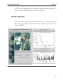
Front cover:
Simulation of parameters for atmospheric correction using the MODO software.
MODO 5
Table of Contents
Table of Contents
Table of Contents ....................................................................................................................................
3
Chapter 1:
Introduction
1.1
1.2
1.3
1.4
1.5
1.6
Goals of MODO ................................................................................................................ 5
Functionality ..................................................................................................................... 6
Limitations ........................................................................................................................ 7
Future Extensions ............................................................................................................. 7
Organisation of this Manual .............................................................................................. 8
Installation of the MODO Software................................................................................... 8
Chapter 2:
Background Information
2.1 MODTRAN®-5 and MODO Integration ............................................................................ 11
2.2 Procedures ...................................................................................................................... 13
2.2.1
2.2.2
Data Extraction....................................................................................................
Convolution.........................................................................................................
2.3 File Descriptions .............................................................................................................
2.3.1
Band Model Files..................................................................................................
2.3.2
Solar Irradiance Spectra ........................................................................................
2.3.3
Sensor Response Spectra......................................................................................
2.3.4
Surface Reflectance Files ......................................................................................
2.3.5
Outputs ..............................................................................................................
2.4 Common Elements ..........................................................................................................
2.4.1
Geometry............................................................................................................
2.4.2
Standard Atmospheres .........................................................................................
2.5 Demo Data ......................................................................................................................
2.5.1
Spectral Libraries .................................................................................................
2.5.2
Tape5s ...............................................................................................................
13
14
15
15
16
17
18
18
19
19
20
21
21
21
Chapter 3:
Workflow Examples
3.1 MODTRAN®-5 Setup ....................................................................................................... 23
3.2 At-sensor Radiance Simulation ....................................................................................... 25
3
Table of Contents
3.3
3.4
3.5
3.6
MODO 5
Simulation of Atmospheric Signatures ............................................................................ 29
Simulation of Sensititivity Series ..................................................................................... 30
Evaluation of Sensor Specifications ................................................................................ 31
Simple Atmospheric Correction ....................................................................................... 32
Chapter 4:
Functions Reference Guide
4.1 Generic Menu Elements .................................................................................................. 35
4.1.1
4.1.2
4.1.3
4.1.4
4.1.5
4.1.6
4.1.7
4.2
4.3
4.4
4.5
4.6
4.7
4.8
4.9
The MODO main window ...................................................................................... 35
Help System ........................................................................................................ 36
Text Editing ......................................................................................................... 36
Selecting Albedo Spectra ...................................................................................... 37
Selecting Lambertian Albedo Spectra ...................................................................... 38
Plotting ............................................................................................................... 40
Session Management ............................................................................................ 41
Menu: File ....................................................................................................................... 42
Menu: Edit....................................................................................................................... 47
Menu MODTRAN®-5: Setting up a tape5 ........................................................................ 51
Menu: MODTRAN ........................................................................................................... 60
Menu: Analyze ................................................................................................................ 67
Menu: Calculate .............................................................................................................. 75
Menu: Help...................................................................................................................... 82
Batch Processing ............................................................................................................. 84
4.9.1
Batch Commands (for IDL)..................................................................................... 84
4.9.2
Internal Data Format ............................................................................................. 85
References .................................................................................................................................................
Index .............................................................................................................................................................
4
89
93
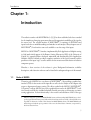
Introduction
Chapter 1
Chapter 1:
Introduction
The radiative transfer code MODTRAN®-51 [2] [3] has been established as de-facto standard
for the simulation of imaging spectrometry data and for quantitative modelling of the signal at
the sensor level. The original interface of MODTRAN®-5 consisting of ASCII-file based
inputs leads often to misunderstandings and mistakes in such analyses. Many frequent users of
MODTRAN®-5 has therefore some tools available to ease the setup of the inputs.
MODO is a MODTRAN®-5 interface, implemented by ReSe Applications Schläpfer starting
in 1996 under initial support of the Remote Sensing Laboratories (RSL) of the University of
Zurich. It is currently further developed, maintained and distributed by ReSe Applications
Schläpfer. MODO includes an almost complete translation of the logical structure and the
parameters of the input ‘tape5’ as well as utilities for the extraction and convolution of radiation
component spectra.
Hereafter, a short overview of the software is given. Background information, workflow
descriptions, and a functions reference can be found in the subsequent chapters of this manual.
1.1
Goals of MODO
The major goal of MODO is to ease the use of MODTRAN®-5 by providing a graphical user
interface (GUI) for the creation of the input files as well as for the analysis of the outputs with
respect to hyperspectral remote sensing. The efforts resulted in the MODO (‘MODTRAN®5 Organizer’) concept. MODO is not only a graphical front-end to the MODTRAN®-5 radiative transfer code but also included advanced scientific processing tools focussing on remote
sensing applications. Its basic functionality is the creation and translation of files of the type
1.
MODO is designed to operate with MODTRAN® features and functionality. MODTRAN® was co-developed by Spectral Sciences Incorporated (SSI) and the United States Air Force (USAF). SSI and USAF are not
responsible for deviations of results of this software from MODTRAN® software. The MODTRAN® trademark is being used with the express permission of the owner, the United States of America, as represented by
the United States Air Force.
5
Chapter 1
Introduction
‘tape5’ or ‘.tp5’. The subsequent processing of output spectra, regarding extraction, conversion
and plotting, can then be done in the same working environment. Additional functionalities
allow the convenient creation of sensitivity analysis series and the convolution of spectra to
hyperspectral band characteristics, but also a simplified atmospheric correction routine.
1.2
Functionality
MODO version 5 includes the following features:
• Import/export of MODTRAN®-5 tape5 ASCII control files
• Creation and dealing with multiple run tape5s
• Editing of own, customized atmospheres
• Import/export of ground reflectance spectra including support for adjacency effect
• Support for ENVITM spectral libraries
• Sensitivity analysis through parameter series
• Series of reflectance spectra
• Direct call of MODTRAN®-5 for Windows and UNIX/Linux/OSX
• Includes original executables of MODTRAN®-5 v5.2.0.0 for Windows and MacOSX/
Linux/Solaris2
• Extraction of radiance/transmittance components from MODTRAN®-5 output (e.g.
tape7)
• Extraction of solar flux data from MODTRAN®-5 ‘.flx’ files
• Plotting of standard MODTRAN®-5 outputs (tape7/flux)
• Convolution of outputs to hyper- (gaussian response) and multispectral sensor
• Simplified atmospheric correction (SACO) routine based on MODTRAN®-5 standard
atmospheric correction outputs.
• Eased sensor simulation with a broad collection of response functions for both airborne
and spaceborne optical and thermal instruments
• Helper applications for visibility determination and solar angles calculation
• Direct online help for each GUI panel and this electronic user manual
The MODO interface design is implemented in view of improving the reliability of simulations for optical remote sensing instruments. This end-to-end solution starts with inclusion and
selection of surface reflectance functions from spectral libraries. Second, the atmospheric
6
Introduction
Chapter 1
parameters most critical to the radiative transfer are to be defined, and third, the components
of the at-sensor radiance shall be produced directly for specific sensor response functions. The
pre-selection of relevant situation parameters is done on experience in various application area.
The integration of the given principles has lead to a comprehensive GUI for setting up
MODTRAN®-5 runs in an efficient manner.
1.3
Limitations
MODO has been developed in view of remote sensing data analysis and simulations. It is limited to the following restrictions:
• MODO is an expert simulation tool which (still) requires some knowledge about radiative
transfer simulation principles.
• BRDF functionality of MODTRAN®-5 is not supported.
• Multi-dimensional look up table generation is not easily feasible through the interface.
• MODO is not a fully-featured atmospheric correction program as it does not consider any
in-image variations of the radiometric conditions.
• No import functions for user defined aerosol phase functions and standard radiosonde profiles are available.
1.4
Future Extensions
The MODO application is under continuous improvement. The following features are options
to be potentially included in future versions of the software (depending on demand):
• Support for BRDF input
• Input of standard radiosonde profiles
• Input of MISR aerosol models
• Sun photometer data analysis
Such features are implemented based on specific requests of licensed end users. Please contact
ReSe, if you have new ideas or wishes to the software or if you’d like to contribute suited IDLbased tools to be included in the processing system.
7
Chapter 1
1.5
Introduction
Organisation of this Manual
This manual is organized as follows:
• This Chapter ’Introduction’.
• The second Chapter ’Background Information’ gives some explanations about specifics of
the MODO application.
• The Chapter ’Workflow Examples’ gives guidelines how to work with MODO interactively. It summarizes tips for working with standard sensor data and how to deal with special cases.
• The Chapter ’Functions Reference Guide’ describes every function of the MODO user
interface and the usage of the interface functions. Finally, the bibliographic references as
well as an index of topics can be found in the Appendix.
Some conventions in the manual:
• Menu commands are given as >File:Restore Status p.45<, with a link to the description page.
• Batch routines and calls on the IDL prompt are written in monotype,
e.g., modo,/norun.
Please read the warning texts which are marked by warning sings on the side-bars carefully.
1.6
Installation of the MODO Software
The distribution of MODO includes platform-specific MODTRAN®-5 exectuables, compiled from the original MODTRAN®-5 code and compatible to all current operating systems
(Solaris/Linux/MacOSX/Windows). The system requirements are:
• IDL 7.0 or higher or the free IDL Virtual Machine (ITT Vis.)
• Solaris, Linux (x86), MacOSX (Intel), or Windows (64/32 bit) operating system
• High processing power for MODTRAN®-5 runs
• Screen size at least 1024x768 pixels
• 1.2 GB free disk space
8
Introduction
Chapter 1
The MODO application installer is available from www.rese.ch/download.html. If you don’t
have access to an official IDL license, the IDL Virtual Machine is available as free distribution
directly from ITTVIS, through www.ittvis.com/idlvm. The MODO installation process is as
follows:
1) Install the IDL virtual machine following the installation instructions provided by RSI(this
step is void, if you have IDL/IDL VM/ or ENVI developer installed).
2) Double click the file modo_installer.sav (on Windows) or enter on Unix/Linux/MacOSX:
idl -vm="modo_installer.sav".
3) Please follow the instructions as displayed during the installation process.
4) For licensing, go to the help menu after starting MODO and choose ‘Identify’ in the menu
>Help:License<. Please email the displayed outputs of this job together with your complete
address and affiliation. You will then receive a license key file within a few days. Let us
know if you need any further assistance or product information.
A free 30 days, fully functional evaluation license key may be issued upon request. After expiration of the license, you will need to acquire a license as described above or on the ReSe homepage. If not, you will still be able to run MODO in demonstration mode, which allows the
handling of MODTRAN®-5 outputs, but does not support running MODTRAN®-5 and
MODTRAN®-5 series.
9
Chapter 1
10
Introduction
Background Information
Chapter 2
Chapter 2:
Background Information
This chapter summarizes some background information about the MODO/MODTRAN®-5
simulation environment.
2.1
MODTRAN®-5 and MODO Integration
The MODTRAN®-5 code as it was provided by the Air Force Geophysics Laboratory (AFGL)
is written in the FORTRAN computing language. It is handled by rigidly formatted ASCII
input files. The tape5 is used for the definition of the atmosphere and the geometry, while the
file ‘spec_alb.dat’ (e.g.) defines the background reflectance characteristics. Other optional
input files concern the solar irradiance or the spectral band model. The direct handling of these
files is very sensitive and requires experience with the code. This also bears the danger of introducing errors in at-sensor data simulations.
The interface is based on the IDL [14] programming language which has been established as
well-adopted standard for hyperspectral image processing. The design has been optimized for
research applications and thus does not support high degrees of automatism, avoiding ‘black
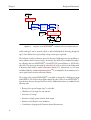
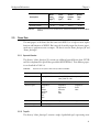
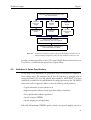
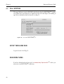
box’ mechanisms. The MODO concept as shown in Figure 2.1 is based on the standard distribution of MODTRAN®-5 by interfacing with the inputs ‘.tp5’ and ‘spec_alb.dat’, and evaluating the outputs ‘tp7’ and ‘.flx’.
One core interface function of the procedure is the tape5 editor window (>Modtran:Setup Tape5
and Run p.60<). It allows to set most of the input parameters using pull-down menus instead of
manually editing the rigidly formatted ASCII file. Logics within the tape5 are considered, such
that if, e.g., the transmittance mode has been selected it is not possible to set the irradiance
source options. Sub-interfaces will pop up for supported special functions such as the import
of user defined atmospheres, the selection of the surface reflectance, or the definition of the four
standard aerosol layers. The interface is grouped in the same way as in the original tape5 to be
consistent with the documentation as provided with MODTRAN®-5. If one or more parameters shall be varied, the setup of multiple run tape5s has proven to be very useful. Each run
11
Chapter 2
Background Information
reflectance
MODO
input preparation
tape5
spec_alb.dat
tape7
MODTRAN
(fortran)
solar flux
MODO
output evaluation
sensor
response
radiance L
plots
convolved L
Figure 2.1:
Integration of the
MODTRAN®-5 standard code with the MODO interface.
within such tape5s can be accessed, edited, or deleted individually by browsing through the
tape5. Some dedicated save options help to keep various tape5s organized.
The inclusion of surface reflectance spectra has become of high importance for modelling atsensor radiance values for known targets. An interface has therefore been included for importing reflectance data into MODTRAN®-5 from ENVI [10] spectral libraries or ASCII reflectance files. The spectra can afterwards be selected for the target as well as for the background,
if adjacency effects shall be studied (>Edit:Import Spectra p.47<). Alternatively, an even more
streamlined function (>Modtran:Reflectance Series p.65<) is included for direct simulation of atsensor signals based on surface reflectance libraries.
The startup of the original MODTRAN®-5 executable is managed by a child process from
within MODO. The code has been slightly adapted in order to allow to use MODTRAN®-5
from whatever directory the tape5 has been saved to. Additional interfaces are included for the
following tasks:
• Plotting of the spectral output (tape7 or solar flux)
• Calculation of solar angles for time and date
• Save/restore of settings
• Extraction of single spectra from the whole output
• Parameter and reflectance series simulation
• Convolution to hyperspectral (Gaussian) channel characteristics
12
Background Information
Chapter 2
• Export of radiance spectra to ENVI spectral libraries
All these utilities have been developed in support of a flexible handling of the MODTRAN®5 inputs and outputs for a fast simulation of at-sensor radiance values. They are described in
detail in Chapter 4 on Page 35.
2.2
Procedures
MODO by itself is only an interface to MODTRAN. The MODTRAN®-5 code has been desribed in detail elsewhere [2] [3] [8], whereas a full description is available commercially through
www.ontar.com. The functionality which is specific to MODO is related to data extraction
and convolution but also the translation of the inputs into ‘human readable’ graphical elements.
The standard wavenumber reference of MODTRAN®-5 is [cm-1]. In VIS/NIR spectrometry
(and optical remote sensing) the standard wavelength reference is [nm] and therefore, some
conversion is required. MODTRAN®-5 by itself also offers a unit conversion and convolution
option which is fully independent from the options as implemented within MODO. The processing workflow within MODO relies on its own extraction, transformation and convolution
routines, which offer some higher flexibility if compared to the implementation in the MODTRAN®-5 code.
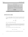
2.2.1 Data Extraction
In normal cases, the total at-sensor radiance is the main output component to be read from the
MODTRAN®-5 outputs. Other components such as the path scattered radiance, specific
transmittance values or the solar irradiation, are of specific interest for atmospheric applications
and correction routines as well as for validation of the cross sensitivity of the simulated spectra
to atmospheric influences. MODO reads the components from the outputs and converts them
to SI standard units [W/(m2 sr nm)] from the original units being [W/(cm2 sr cm-1)]. This conversion is based on the well-known relationship between wavelength λ and wavenumber ν :
1
λ = --- ,
ν
(2.1)
The wavenumber is converted to its equivalent wavelength through the following relationship:
7
10
1
λ [ nm ] = --------------------- = ------- [ nm ] .
–1
ν
ν [ cm ]
(2.2)
13
Chapter 2
Background Information
The relation between the wavelength interval and the wavenumber interval is given by:
1
2
dλ = – ----2 dν and dν = – ν dλ .
ν
(2.3)
The generic relation between the radiance per wavelength L S, λ and the radiance per wavenumber L S, ν is derived from the respective definitions:
2
dφν - .
dφ - ,and with (2.1): L = --------------------dφ - = --------------------L S, ν = --------------------S, λ
dAdΩdν
dAdΩdλ
dAdΩdν
(2.4)
The unit conversion is derived as follows, where L S, λ , and L S, ν denote data values for the
same radiance equivalents and ν the wavenumber value in inverse centimeters:
W W ( cm )
2
L S, λ -----------------= ν L S, ν -----------------------------=
2
m srnm
cm 2 sr ( cm –1 )
–1
W
2
4 W ( cm )
- = ν 2 L S, ν 10 –3 -----------------ν L S, ν 10 -------------------2
2
m sr
m srnm
–1 2
.
(2.5)
The standard unit in [cm-1] is given as the original MODTRAN®-5 wavenumber reference
which may be related closely to the energy levels of the simulated photons. But in imaging spectrometry and spectroscopy of the visible/near infrared part of the spectrum, the most common
wavelength references are microns or nanometers. As the resolution of typical VIS/NIR imaging spectrometers is in the range of 1to 20 nm, it has been decided to select the wavelength in
nanometers as generic reference for data simulation within MODO.
(Compare function: >Modtran:Extract Spectra p.69<.)
2.2.2 Convolution
The MODTRAN®-5 data usually is derived in wavelength units using a triangular slit for convolution to the original band data. Since version 3.7 of MODTRAN, an option is included
which allows the direct convolution of the MODTRAN®-5 outputs to sensor specific response
functions. This option is not fully supported within MODO. A separate convolution function
convolves extracted and possibly joined spectra to sensor characteristics using a Gaussian
approximation of the sensor function or explicite response functions. This option leaves higher
flexibility for research purposes if, e.g., the response function needs to be varied. The convolved
radiance values L i in a band i are calculated as:
14
Background Information
Chapter 2
∫ L S ( λ )r i ( λ ) dλ ∑j L S ( λ j )r i ( λ j )Δλ-j ,
L i = -------------------------------------- ≈ ---------------------------------------------∑j r i ( λ j )Δλ j
∫ r i ( λ ) dλ
(2.6)
where r j ( λ ) is the spectral response function of the sensor’s band. A stepwise assumption is
taken for the convolution if the number of raw data values j is sufficient within the width of
the spectral band. If the original resolution is not sufficient, a polynomial is calculated through
the original data points L s ( λ j ) for better approximation of the spectrum and summarized
through a number of k = 100 interpolated data points, i.e:
∑k Poly ( L S ( λ j ) ) k r i ( λ k )Δλ k
-.
L i ≈ -------------------------------------------------------------------∑ r i ( λ k )Δλ k
(2.7)
k
A minimal number of 2 data points within the range of the target bands is required for a sufficient calculation of the convolved data values in any case.
(Compare function: >Modtran:Extract Spectra p.69<.)
2.3
File Descriptions
The data basis for the MODTRAN®-5 calculation is provided together with the MODTRAN®-5 code. MODO contains some additional data for more complete simulation posssibilities, which are described in Chapter 2.5 on Page 21. An overview over the files provided by
MODTRAN®-5 and their locations within the installation as described in the original
MODTRAN®-5 user’s manual [2] is given below.
2.3.1 Band Model Files
The variable ‘MODTRN’ in the 1st position in CARD 1 (see Table 4.1 on Page 55) selects the
band model algorithm used for the radiative transfer, either the moderate spectral resolution
MODTRAN®-5 band model or the low spectral resolution LOWTRAN band model.
LOWTRAN spectroscopy is obsolete and is retained only for backward compatibility. The
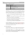
MODTRAN®-5 band model may be selected either with or without the correlated-k treatment. The values for band model determination in ‘MODTRN’ (f are given in Table 2.1.
15
Chapter 2
Background Information
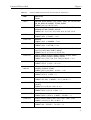
Table 2.1:
‘MODTRAN’ band model options.
‘MODTRN’ values
Band model
‘T’, ‘M’ or blank
MODTRAN®-5 band models
‘C’ or ‘K’
MODTRAN®-5 correlated-k option (IEMSCT radiance modes only;
most accurate but slower run time).
‘F’ or ‘L’
20 cm-1 LOWTRAN band model (not recommended except for quick
historic comparisons).
MODTRAN®-5 uses a default 1 cm-1 band model, but if variable ‘LBNAM’ in CARD 1A is
set to ‘T’, the file name of a 0.1 cm-1, 5 cm-1 or 15 cm-1 band model will be read from variable
‘BMNAME’ in CARD 1A2. MODTRAN®-5 will open the corresponding 0.1 cm-1, 1 cm-1,
5 cm-1 or 15 cm-1 Correlated-k data file when input variable ‘MODTRN’ equals ‘C’ or ‘K’.:
• ‘p1_2008’: The 0.1 cm-1 band model file is used for highest accuracy (at the cost of long
run times) The name of the accordant CK data file is hardwired to ‘DATA/
CORKp1.BIN’.
• ‘01_2008’: The 1 cm-1 band model file is used if no other file is specified. The name of the
accordant CK data file is hardwired to ‘DATA/CORK01.BIN’.
• ‘05_2008’: The 5 cm-1 band model allows faster short-wave calculations. The name of the
accordant CK data file is hardwired to ‘DATA/CORK05.BIN’.
• ‘15_2008’: The 15 cm-1 band model allows fastest short-wave calculations. The name of
the accordant CK data file is hardwired to ‘DATA/CORK15.BIN’.
In MODO’s MODTRAN®-5 base widget described in >Modtran:Setup Tape5 and Run p.60<,
the alternative band models described above are selected by switching ‘1 cm-1 Standard’ in the
second frame to ‘Special Bandmodel’. When calculating >Modtran:At-Sensor Signal p.61<, a
choice of band models is available in the first frame.
2.3.2 Solar Irradiance Spectra
If variable ‘LSUNFL’ in CARD 1A is set to ‘F’ or left blank, a default solar reference based on
Kurucz data is selected. The spectral resolution is adapted to the selected band model file.
If variable ‘LSUNFL’ in CARD 1A is set to ‘T’, ‘USRSUN’ in CARD 1A1 is used to define
the top of atmosphere (TOA) solar irradiance database. If a number is set, the file is selected
according to Table 2.2. The solar databases provided by MODTRAN®-5 are obtained from
various sources [1] [6] [7] [17] [18] [19] [20] [39] [40] [43].
16
Background Information
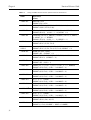
Table 2.2:
Chapter 2
Listing of solar irradiance databases defined by ‘SUNFL2’.
‘LSUNFL’ values
Solar irradiance database
1
The corrected Kurucz database is used (DATA/SUN01kurucz2005.dat).
2
The Chance database is used (DATA/SUN01chkur.dat).
3
The Cebula plus Chance data are used (DATA/SUN01cebchkur.dat).
4
The Thuillier plus corrected Kurrucz data are used (DATA/
SUN01thkur.dat).
5
The Fonenla data are used (DATA/SUN01fontenla.asc).
6
The Kurucz 1997 data are used (DATA/SUN01kurucz1997.dat).
7
The Kurucz 1995 data are used (DATA/SUN01kurucz1995.dat).
T or t
A user-defined database residing in the file is used.
The user-defined file must be in a special form. The first line must contain a pair of integers.
The first integer designates the spectral unit [1 for frequency in wavenumbers (cm-1); 2 for
wavelength in nanometers (nm); and 3 for wavelength in microns (μm)]. The second integer
denotes the irradiance unit [1 for Watts cm-2, 2 for photons sec-1 cm-1/nm; and 3 for Watts
m-2/μm or equivalently milli-watts m-2/nm]. The subsequent lines contain one pair of frequency and irradiance entry per line. There is no restriction on frequency or wavelength increments. However, data beyond 50’000 wavenumbers are ignored. If needed, data in the usersupplied file are padded with numbers from ‘newkur.dat’ so that the data encompasses the
range of 50 to 50’000 wavenumbers.
The user-defined file has a form that is different from the files in the DATA directory.
2.3.3 Sensor Response Spectra
If variable ‘LFLTNM’ in CARD 1A is set to ‘T’, CARD 1A3 is used to select a user-supplied
instrument filter (channel) response function file.
Sample AVIRIS (‘DATA/aviris.flt’) and LANDSAT7 (‘DATA/landsat7.flt’) filter response
functions are supplied with MODTRAN. MODO comes with additional sensor response data
for a broad range of sensors, which are stored in the directory ‘sensor_resp’. However, the
response files provided with MODO use a different file format than Modtran.
For more detailed information on sensor response file formats, see >Analyze:Plot Response
Function p.44<.
17
Chapter 2
Background Information
2.3.4 Surface Reflectance Files
The variable ‘SALBFL’ in CARD 4L1 contains the name of the input data file being used to
define the spectral albedo. The default spectral albedo file ‘DATA/spec_alb.dat’ may be used
or a user-supplied file. If a user-supplied file is specified, it must conform the following criteria,
which are stated in the original ‘DATA/spec_alb.dat’:
• Lines beginning with an exclamation mark ‘!’ are ignored. Comments after an exclamation
mark are also ignored.
• Each surface is defined by a positive integer label, a surface name, and its spectral data. The
integer label and surface name must appear as a pair on a header line with the integer label
followed by a blank.
• Header lines must not include a decimal point ‘.’ before an exclamation mark, and spectral
data must include a decimal point.
• Spectral data is entered with one wavelength (in microns) and one spectral albedo per line,
separated by one or more blanks. The spectral wavelengths for each surface type must be
entered in increasing order. The spectral albedos should not be less than 0 or greater than
1.
• The first 80 characters of each line are read in.
The variable ‘CSALB’ in CARD 4L2 defines the number or name associated with a spectral
albedo curve from the ‘SALBFL’ file. There are currently 46 spectral albedo curves available in
the default spectral albedo file ‘DATA/spec_alb.dat’.
Also note that the file ‘DATA/spec_alb.dat’ has to be overwritten in order to use different spectra than the standard selection.
2.3.5 Outputs
The standard MODTRAN®-5 output files tape6, tape7 and tape8 are described in >Modtran:Setup Tape5 and Run p.51<.
MODO generates additional outputs, mostly in columnar ASCII format:
• >Edit:Import Spectra p.47<: The imported data is written to a file with the input file’s header
information marked out with exclamation marks. If multiple spectra are selected, the spectra are vertically listed one after another with their specifications in a title row, followed by
two columns containing reference wavelengths and radiance or reflectance values. This format is not suitable as input for >File:Quick Plot p.44< or >Edit:Labels and Columns p.49<, as
they require an input with horizontally stored value columns referring to the same refer18
Background Information
Chapter 2
ence wavelength column. Use >File:Edit Textfile p.47< and >Modtran:Append Spectra p.73< to
produce ASCII files containing multiple spectra listed horizontally.
• >Edit:Labels and Columns p.49<: The output ASCII file has the same row/column format as
it is displayed in the editing widget. There are no comments marked out, but only one title
row containing the column labels. The radiance or reflectance values for each spectrum are
listed horizontally, all referring to the same reference wavelength in the first column. The
output can be plotted in >File:Quick Plot p.44<.
• >Modtran:Extract Spectra p.69<: The output ASCII file has the same row/column format as
outputs from >Edit:Labels and Columns p.49<. There are no comments marked out, but only
one title row containing the column labels. The radiance or transmittance values for each
spectrum are listed horizontally, all referring to the same reference wavelength in the first
column. The output can be plotted in >File:Quick Plot p.44<.
• >Modtran:Append Spectra p.73<: The output ASCII file has the same row/column format as
outputs from >Edit:Labels and Columns p.49<. There are no comments marked out, but only
one title row containing the column labels. The radiance or reflectance values for each
spectrum are listed horizontally, all referring to the same reference wavelength in the first
column. The output can be plotted in >File:Quick Plot p.44<.
2.4
Common Elements
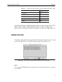
2.4.1 Geometry
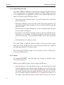
The geometric conventions for the standard angles used in MODTRAN®-5 are given in
Figure 2.2.
19
Chapter 2
Background Information
Figure 2.2:
Geometric conventions used in the
MODTRAN®-5 code and MODO inter-
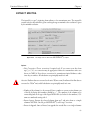
2.4.2 Standard Atmospheres
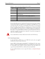
The total water vapor column in the atmosphere varies strongly worldwide. It ranges from
almost zero at high altitude stations and in polar regions, and up to 4 cm in tropical climates.
The single standard atmospheres given in the radiative transfer codes represent a wide variety
of water vapor content which is given in Table 2.3. This standard situations have to be used for
radiance simulations if no in-situ values are available.
Water
Vapor
[kg/m2]
Ozone
column
[g/m2]
Tropical
41.98
Midlatitude Summer
Ground
Pressure
[hPa]
Ground
Temp.
[ C]
5.43
1013.0
26.85
29.82
6.95
1013.0
20.85
Subarctic Summer
21.20
7.50
1010.0
13.85
US Standard
14.39
7.48
1013.0
14.95
Atmosphere
Table 2.3:
20
Integral characteristics of the McClatchey standard atmospheres, as stored in MODTRAN®-5 .
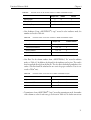
Background Information
Chapter 2
Water
Vapor
[kg/m2]
Ozone
column
[g/m2]
Midlatitude Winter
8.67
8.64
1018.0
-0.95
Subarctic Winter
4.23
10.40
1013.0
-16.05
Atmosphere
Table 2.3:
2.5
Ground
Pressure
[hPa]
Ground
Temp.
[ C]
Integral characteristics of the McClatchey standard atmospheres, as stored in MODTRAN®-5 .
Demo Data
The main purpose of the demo data that comes with MODO, is to help new users explore
functions and limitations of MODO. But it may also be useful as input data for more experienced users, to perform test runs or compare . The data is stored in ‘/demo_data/spec_lib’ and
‘/demo_data/tape5’.
2.5.1 Spectral Libraries
The directory ‘/demo_data/spec_lib’ contains two additional spectral libraries from ATCOR
and S6 to complement the spectral data provided in MODTRAN®-5. Their different properties are described in Table 2.4.
Table 2.4:
Properties of the spectral demo data provided with MODO.
MODTRAN®-5
ATCOR
S6
File name
‘spec_alb.dat’
‘atcor_ASCII_lib.txt’
‘atcor_lib.sli’ & ‘.hdr’
spectra_6s.txt
Number of surfaces
46
20
3 standard cases
Surface types
Vegetation
Soil
Urban
Artificial
Snow
Ice
Sea
Vegetation
Agriculture
Concrete
Sea
Lake
Vegetation
Sand
Lake
Spectral resolution
(mostly low)
high
high
Spectral range
(mostly large)
300-2600 nm
350-2600 nm
2.5.2 Tape5s
The directory ‘/demo_data/tape5’ contains a couple of predefined tape5s representing exem21
Chapter 2
Background Information
plary parameter sets for different types of atmospheric situations. They serve as examples for
different simulation types processible in MODO and can easily be customized to new, userdefined tape5s.
• ‘radiance.tp5’: calculates total, scattered and reflected radiances from a field observers view.
Default ‘Ground Altitude’ is 100 m. Display the output file ‘radiance.tp7’ with >Modtran:Plot Tape7 Output p.67<.
• ‘irradiance.tp5’: calculates the solar irradiance on a certain day of the year (default=150)
and the atmospherical transmittance for a common combination of atmospherical parameters. Display the output file ‘irradiance.tp7’ with >Modtran:Plot Tape7 Output p.67<.
• ‘flux.tp5’: calculates the solar flux for a common combination of atmospherical parameters. The default spectral range accounted for is limited to a narrow portion in the 2500
nm region. The output up- and downward irradiances in the file ‘flux.flx’ can be displayed
with >Modtran:Plot Solar Flux p.68<. Enter a positive value in the field ‘Ground Altitude’.
• ‘radiosonde.tp5’: this is a working example file containing five layers of radiosonde data.
Please use a text editor (or maybe modo) to add additional layers according to the MODTRAN®-5 standard (sorry, modo does not yet support any more sophisticated tools for
radiosonde data import).
• ‘radiosonde_trans.tp5’: another example file with radiosonde profile, this time for transmittance calculation
• ‘sensor0_demo.tp5’: this is a copy of the file ‘sensor0.tp5’ which is the basis for the first
option (low resolution, standard MODTRAN®-5 settings) in the at-sensor radiance simulator widget (>Modtran:At-Sensor Signal p.61<).
• ‘sensor1_demo.tp5’: this is a copy of the file ‘sensor1.tp5’ which is the basis for the second
option (high resolution, standard MODTRAN®-5 settings) in the at-sensor radiance simulator.
• ‘sensor2_demo.tp5’: this is a copy of the file ‘sensor2.tp5’ which is the basis for the third
option (high resolution, DISORT scattering) in the at-sensor radiance simulator.
• ‘sensor3_demo.tp5’: this is a copy of the file ‘sensor3.tp5’ which is the basis for the fourth
option (high resolution, DISORT scattering, correlated-k) in the at-sensor radiance simulator. Please use with care as it requires quite some processing time.
• ‘spectral.tp5’: calculates radiance using a preset spectral reflectance (meadow from the standard spectral albedo file).
22
Workflow Examples
Chapter 3
Chapter 3:
Workflow Examples
MODO is a scientific workbench which does not rely on one typical use case. It contains tools
to ease the creation of MODTRAN®-5 input tapes and for the extraction and further treatment of their outputs. The typical workflow using the MODO utility depends on the task to
be performed. It rather supports a broad variety of potential applications of the MODTRAN®5 code. The MODO user interface to MODTRAN®-5 is a tool for the forward modeling task
which so far has been in use by various expert users. Hereafter, workflows and examples for simulating the at-sensor radiance for standard remote sensing situations and other typical use cases
are explained.
The software contains a complete operational MODTRAN®-5 installation. Starting MODO
is done by opening the file 'modo.sav' from within IDL or through the free IDL Virtual
Machine (typing ‘modo’ on the IDL prompt will work as long as the file is found by IDL).
Note that the herein mentioned functions are explained in detail on the indicated pages in the
subsequent Chapter ’Functions Reference Guide’.
3.1
MODTRAN®-5 Setup
The first workflow describes the usage of MODTRAN®-5 in its standard mode through the
MODO GUI. This workflow is recommended for experienced MODTRAN®-5 users and for
people who require the full MODTRAN®-5 feature set. This standard workflow for MODTRAN®-5 operations is as follows:
1) Choose >Modtran:Setup Tape5 and Run p.60<. Be aware that for an instance, the corresponding tape5 editor window will confuse a first time user, but together with the MODTRAN®-5 user manual, it will become manageable to fill in senseful values here.
2) Choose your old tape5 or define a name of a new tape.
3) Make your setting in the appearing huge tape5 window. Multiple runs are allowed (use
23
Chapter 3
Workflow Examples
arrows to switch). The window adjusts dynamically according to the selected options.
4) Use the help for this window for further informations or open the MODTRAN®-5 manual with >Help:Browse Manual<, as described in Section 4.1.2 on Page 36 (the manual follows the same logic/order as the displayed window).
5) Now, the tape may be stored for future use.
After setting all parameters, MODTRAN®-5 is invoked directly or the tape is stored to the
MODTRAN®-5 directory. Maybe this leads to a good end and a MODTRAN®-5 output is
now created.
After the surface reflectance has been defined, the various parameters need to be set in the tape5
window. One may choose to vary certain parameters and create a multiple run tape5. At this
point, additional knowledge of the geometric and meteorologic situation to be simulated is
required. Furthermore, some basic comprehension of the MODTRAN®-5 functionality helps
to create inputs to MODTRAN®-5 making physical sense.
MODTRAN®-5 can be run afterwards in one of its four major modes, which are radiance,
transmittance, solar irradiance, or thermal radiance. Depending on the settings for the DISORT option and the wavelength resolution, such runs may be very time consuming for the
radiance mode. The first run in the standard output tape7 or in the optionally created ‘.flx’ file
may be plotted directly afterwards for quick visualization of the outputs.
Inputs:
• >Edit:Import Spectra p.47<: Imports external reflectance spectra and converts them to the
MODTRAN®-5 internal data format (such as foreseen in ‘spec_alb.dat’), which may be
accessed for simulations.
Functions:
• >Edit:Labels and Columns p.49<: Changes the labels of the single spectra and deletes columns
in spectral ASCII files.
• >Modtran:Run from Tape5 p.60<: This function allows to run any user-defined input tape5
using MODTRAN. The tape5 may be edited externally from MODO, which is specifically suited if functionality not supported by MODO shall be used.
• >Modtran:At-Sensor Signal p.61<: If at-sensor signals shall be simulated in an easy way, this
function helps to ease the processing workflow. MODTRAN®-5 is run, the selected radiance/transmittance component is extracted and the output is directly convolved to selected
sensor characteristics.
• >Analyze:Extract Spectra p.69<: Extracts single spectra out of tape7 outputs, works also on
24
Workflow Examples
Chapter 3
multiple MODTRAN®-5 runs (have a look at the corresponding help page there).
• >Modtran:Append Spectra p.73<: Appends spectral ASCII files to one single file.
• >Calculate:Convolution p.77<: Convolves the MODTRAN®-5 spectra (even appended ones,
as many columns as desired) to hyperspectral channel characteristics. A Gaussian shape of
the channels response function is assumed for this calculation.
• >Calculate:Shifttest Convolution p.78<: To be used if you want to test the impact of a known
spectral channel shift on the convolution results.
Outputs:
• >File:Show Textfile p.42<: Prints the whole ASCII output in the utility window (this basic
text window has a suitable size to study tape6/7/8 outputs without double lines etc.). See
Chapter 4.1.3 on Page 36.
• >File:Quick Plot p.44<: Shows extracted columnar ASCII files in a default plot window.
• >Edit:Export Spectra p.49<: Allows to export any created/extracted spectral data to ENVI
spectral libraries, whereas the standard spectral ASCII files can be easily imported into
spreadsheet programs.
• >Modtran:Plot Tape7 Output p.67<: Plots the whole output (from the tape7).
• >Modtran:Plot Solar Flux p.68<: Plots the solar flux file.
3.2
At-sensor Radiance Simulation
In imaging spectroscopy, the normal case starts with known surface reflectance spectra which
need to be transposed to at-sensor radiance values. For the creation of spectral databases or
look-up-tables (LUTs) for later inversion, standard setting for reflectance and discrete values
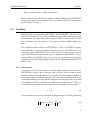
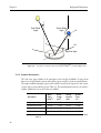
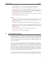
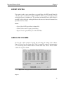
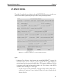
for parameter variation are taken as basic input. An overview of a typical data simulation workflow is given in Figure 3.1.
The at-sensor radiance is the critical parameter for the physical investigation of imaging spectrometry data. It is derived by calibration of a sensor system and needs to be compared to the
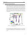
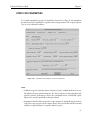
expected radiance levels. An example of simulated at-sensor radiance components is shown in
Figure 3.2. The components of the signal are to be considered for validation of the relative sensitivity of the radiance to atmospheric and surface parameters. Usually, a series of simulations
needs to be set up in order to obtain the variation of the signal. This approach may be chosen
to simulate the expected at-sensor radiance levels to be constructed.
The core interface of the MODO procedure is the tape5 editor window described in Chapter
4.4 on Page 51. It allows to set most of the input parameters using pull-down menus instead
25
Chapter 3
Workflow Examples
Import Surface Reflectance Spectra from SLI / ASCII
®
Edit Tape5 Input to MODTRAN
-5
®-5 (radiance/transmittance/irradiance)
Run MODTRAN
Plot tape7 or
Spectrum Extraction
solar flux output
and Conversion
Plot spectrum or
convolved spectrum
Convolve to Gaussian
spectral response functions
Simulated sensor-specific
radiance/transmittance/flux
26
Figure 3.1:
Typical workflow structure used for the simulation of imaging spectrometer data.
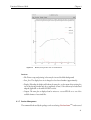
Figure 3.2:
Total at-sensor radiance over vegetation convolved to specifications of the APEX
instrument and to reference instruments (AVIRIS, HYMAP, and DAIS 7915).
Workflow Examples
Chapter 3
of manually editing the rigidly formatted ASCII file. However, the various input options to
MODTRAN®-5 may be misleading if a fast result of at-sensor signals is to be calculated. Thus,
a streamlined version of this window has been created. It uses four standard processing options,
which allow the trade-off between processing accuracy and speed. The indicated approximative
time is given for the radiance simulation of one hyperspectral standard situation on a 1.5 GHz
machine.
• Low resolution: (4 seconds)
• High resolution: (1 minutes)
• High resolution with DISORT multiple scattering algorithm (5 minutes)
• High resolution with DISORT and correlated-k approach (3-4 hours - not to be recommended.).
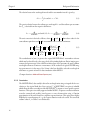
Despite the differences in speed, this four standard options exhibit significant differences of the
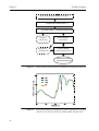
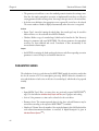
simulated radiance values, specifically within or at the edges of atmospheric absorption features. A non-respresentative example is given in Figure 3.3, where the deviations of the first
three methods from the most accurate option is shown. Differences inherent to the MODTRAN®-5 radiative transfer code are found which are at up to 5% in standard cases but may
even be higher when strong absorption is present.
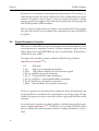
Furthermore, the parameters most often used for simulations have been selected from the standard options. All cloud options have been omitted as they usually are not required – nor desired
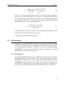
– for imaging spectrometry applications. The respective workflow from standard situations to
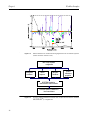
at-sensor radiance is depicted in Figure 3.4. It includes the extraction of the at-sensor radiance/
irradiance or transmittance and a convolution to the selected sensor response function.
The graphical implementation groups the four main inputs to >Modtran:At-Sensor Signal p.61<
‘atmosphere’, ‘surface’, ‘geometry’, and ‘sensor’ together in frames.
27
Chapter 3
Workflow Examples
Figure 3.3:
Relative difference of standard scattering algorithms from correlated-k approach
(dotted: at-sensor radiance curve).
MODTRAN standard
configuration
atmospheric
conditions
sensor
response
geometric
conditions
surface
reflectance
properties
MODTRAN simulation
data extraction and convolution
at-sensor radiance, irradiance or
total transmittance
Figure 3.4:
At-sensor radiance simulation workflow with 4 input sections based on standard
MODTRAN®-5 configurations.
28
Workflow Examples
3.3
Chapter 3
Simulation of Atmospheric Signatures
The most straight-forward simulation of atmospheric signatures using MODTRAN®-5 is the
calculation of the transmittance of a specific optical path (see example of such an output in
Figure 3.5). Transmittance curves are derived for the characterization of atmospheric scatterers
and gases such as water vapor [33]. Anyhow, the transmittance runs do not include all effects
of multiple scattering on the path. It is thus preferred to use radiance simulations under well
known atmospheric parameter variations for realistic results. At-sensor radiance values are then
evaluated with respect to the variation of atmospheric parameters available within MODTRAN®-5 such as the visibility, cirrus or cloud coverage, humidity, and ozone content or with
respect to geometric constraints such as sensor altitude, ground altitude, sun zenith angle, or
sensor zenith angle.
Figure 3.5:
Simulation of atmospheric transmittance using the direct transmittance calculation - Standard MODO output.
Such variations may be combined for building LUTs for atmospheric correction as it has been
done within the ATCOR programs [25] [28]. The MODO interface does not support directly
the construction of such look-up-tables but its internal functionality can be used to ease their
creation.
29
Chapter 3
3.4
Workflow Examples
Simulation of Sensititivity Series
For sensitivity analysis, the workflow is as follows:
1) Define a tape5 according to your standard situation (use the above described procedure for
that task).
2) Save the tape5 as basis for further operation.
3) Use one of the following functions and select the created tape5 as basis:
>Modtran:Parameter Series p.64<: For sensitivity analysis, a tape5 can be used as a basis to
create series of spectra, while changing one parameter systematically.
>Modtran:Reflectance Series p.65<: Analogous to the above function, a spectral library can
be taken as series input for a simulation here.
4) Export the results for further analysis.
Sensitivity analysis usually requires the creation of series of radiative transfer calculations, where
one specific parameter under question is varied systematically. A dedicated tool for this task is
therefore of common interest, triggering MODTRAN®-5 to perform a number of calculations
at once. The MODTRAN®-5 output is then parsed for the searched radiance (or irradiance/
transmittance, respectively) component which leads to a series of outputs compiled in one singular output file. The respective workflow is given in >Modtran:Parameter Series p.64<. The
parameters currently included are:
• Visibility (aerosol optical thickness) and aerosol model (standard models only)
• Standard atmospheres
• Gases: Water vapor, ozone, carbon dioxide
• Geometry: Viewing zenith, sun zenith, relative azimuth
• Sensor height and ground altitude
• Surface reflectance
For user friendliness, the inclusion of spectral libraries as parameter-series option has been
implemented in a separate GUI, as it requires an additional side input by interfacing to the
spectral libraries. The output may be the default total radiance/transmittance, but also components such as path radiance or direct reflected radiance may be chosen for more specific analysis.
The appearance of the related GUIs is depicted in the function >Modtran:Parameter
Within a predefined standard situation (tape5), one parameter can be varied by
Series p.64<.
30
Workflow Examples
Chapter 3
s ta n d a rd s itu a tio n /p a ra m e te rs fro m
p re -d e fin e d ta p e 5
a e ro s o l/
tra c e g a s
ra n g e
a n g u la r/
a ltitu d e
ra n g e
s p e c tra l
lib ra ry
a tm o s p h e ric
s e rie s
g e o m e tric
s e rie s
s u rfa c e
re fle c ta n c e
s e rie s
M O D T R A N s im u la tio n
d a ta e x tra c tio n a n d c o n v o lu tio n
a t-s e n s o r ra d ia n c e , irra d ia n c e o r
to ta l tra n s m itta n c e s e rie s
Figure 3.6:
Workflow for sensitivity analysis. A series of calculations is created from a predefined standard configuration, where only one parameter is varied at a time.
providing a comma separated list of entries. The output is finally directly convolved to the sensor of interest as selected from the internal sensor response library.
3.5
Evaluation of Sensor Specifications
For the design of new instruments, the specifications need to be fixed based on simulated atsensor radiance values. The simulations may be done by comparison to measured values of
existing instruments [32] or by fully physical based simulation. MODTRAN®-5 has been
established as a standard tool for such simulations for imaging spectrometry data. The MODO
utility can be used in a supportive manner to derive the following critical parameters:
• Typical and extreme at-sensor radiance levels
• Application-specific reflectance based signal (delta radiance) simulations
• Noise equivalent delta radiance specification
• Spectral resolution (FWHM)
• Spectral sampling interval requirement
Full width half maximum (FWHM) spectral resolution and spectral sampling interval are
31
Chapter 3
Workflow Examples
derived by series of convolutions to potential spectral response functions. The sensitivity, e.g.,
within absorption features, may then be characterized to derive recommendations for spectral
resolution. An example is given in Figure 3.2, where the spectral characteristics of existing
imaging spectrometers are compared to potential resolution specifications of the upcoming Airborne Prism Experiment (APEX) instrument.
However, the presented approach does not compare to measured data values. If the real signals
after optics and electronics are to be simulated, more sophisticated tools such as SENSOR [4]
are required.
3.6
Simple Atmospheric Correction
With version 5 of MODTRAN, an optional side output has been introduced which stores the
essential parameters for atmospheric correction. Using these parameters together with some
further outputs from a single MODTRAN run with zero spectral albedo, all information is
available for inversion, which is:
The outputs of the atmospheric parameter calculation in MODO using the function
Modtran:Atmo-Cor Parameters p.63 are:
wvl
Wavelength
L_atm
Single scattered atmospheric path radiance
E_0/d^2
TOA irradiance divided by the earth-sun distance squared
T_dif_sun_gnd diffuse sun-ground transmittance
T_dir_tot Sun-ground-observer direct transmittance
T_dif_obs_gnd Observer - ground embedded diffuse transmittance
T_dir_obs_gnd Observer - ground direct transmittance
S_albedo
Spherical Albedo of the atmosphere from ground
The first two parameters are derived from the zero albedo run, whereas all transmittances and
the spherical albedo are extracted from the *.acd atmospheric correction data output. The eight
column of the output are stored in a text file with one data set per spectral band of the selected
instrument.
In a second step, these parameters are directly applied to a calibrated image data file using the
function Calculate:Simple Atmo-Cor p.79. The data file is to be provided in ENVI file format,
whereas a calibration file with the parameters c0 and c1 for each spectral bands have to be provided.
32
Workflow Examples
Chapter 3
The correction uses the standard atmospheric correction equation which first calculates the
apparent top of atmosphere reflectance as:
πd ( ( c 1 DN + c 0 ) ⁄ 100 – L atm )
ρ∗ = ----------------------------------------------------------------------,
E 0 cos θ
2
(3.1)
and therefrom the surface reflectance is derived using the standard atmospheric correction formulation by Vermote [41] as:
ρ∗
ρ = -----------------------------------------------τ tot, dir + τ dif, obs + sρ∗
(3.2)
The path scattered radiance can be derived in the multiple scattering case:
E 0 cos θτ tot, dir τ dif, obs
L path = L atm + -------------------------------------------2
πd ( 1 – sρ a )
(3.3)
The adjacency reflectance ρ a is in a first iteration assumed to be constant and if the adjacency
correction option is selected, it is replaced in a second iteration by the spatially smoothed reflectance of the first result.
The such derived ouput is a spectral albedo from calculation point of view, ie. all MODTRAN
parameters are derived assuming lambertian reflectors. However, the real remote sensing quantity is truly directional and thus the output may be best described as a directional-hemispherical
quantity, being a mixture between the HDRF for the diffuse irradiance portion of the data and
a weighted integration of the BRF for the directional irradiance part of the irradiance as
described in the original definitions document by Nicodemus 1977[22].
33
Chapter 3
34
Workflow Examples
Functions Reference Guide
Chapter 4
Chapter 4:
Functions Reference Guide
4.1
Generic Menu Elements
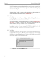
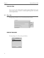
4.1.1 The MODO main window
Figure 4.1:
The MODO main menu.
35
Chapter 4
Functions Reference Guide
The MODO main menu at the top of the main window is used for interactive operation of the
software. It consists of 4 major menu items (see Figure 4.1), which are described beginning
with Section 4.2 on Page 42.
The button ‘Reload Text File’ at the botton of the window allows to update the display of a
text file which had been selected by the function >File:Show Textfile p.42<
4.1.2 Help System
Each MODO window interface has its own help text, which can be displayed by the corresponding ‘Help’-Buttons (compare Section 4.8 on Page 82).
The official MODTRAN®-5 manual can be browsed with the command >Help:Browse MODTRAN Manual p.83< command. It is located as PDF file (‘Modtran_Manual.pdf’) within the
MODO installation (please open directly if it does not open from the menu).
An in-depth description of some aspects of MODTRAN is included in the file
‘MODTRAN_Report.pdf”, included in the DVD distribution of MODO.
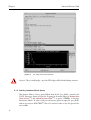
4.1.3 Text Editing
Any ASCII formatted data file or description may be edited directly through the MODO builtin small text editor (see Figure 4.2). The editing tool is a convenient way to browse and edit
ASCII files on the current working directory (e.g to look at an ENVI Header or at some ASCII
auxiliary data), but also to check auxiliary data streams.
Figure 4.2:
36
Menu tasks of the MODO text editor.
Functions Reference Guide
Chapter 4
Actions
• Save: Save changes to the file.
• Save As: Saves the file to a different name.
• Print Setup: Sets up the printer depending on your operating system.
• Print: Prints the file.
Attention: While printing, files of multiple pages are separated into a series of print jobs with
one page per print job. This may cause problems for large files since your printer queue may be
overloaded. Please use dedicated text processing routines for printing large text files.
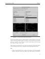
4.1.4 Selecting Albedo Spectra
This function allows to select a spectral albedo from the file ‘spec_alb.dat’, situated in the
‘DATA’ directory as shown in Figure 4.3. It appears in the menu widgets of >Modtran:Setup
Tape5 and Run p.51< and >Modtran:At-Sensor Signal p.61< as option ‘>Spectr<‘ in the dropdown
menu ‘Albedo’. In order to feed your own spectra, replace the input file 'spec_alb.dat' with an
own creation. MODTRAN®-5 can be run first in order to have the spectral reference available.
Input
• >Change< Spectral Albedo File: the currently active file is shown. Its file format should be
conform to the format of the file ‘spec_alb.dat’ in the ‘DATA’ directory of the MODTRAN®-5 installation. The names of all available spectra appear in the list. Changing the
spectral albedo file replaces the current file spec_alb.dat in the DATA directory, whereas
the replaced file is moved to spec_alb_old.dat.
NOTE: on unix/linux/macOSX systems, the spectral albedo file in the DATA directory is
not overwritten, but the selected file name is passed to MODTRAN®-5 as a special parameter.
Functions
• Selecting one of the spectral albedos from list reads the data for the selected spectrum from
the spec_alb.dat file and plots a preview in the window below.
• The upper limit of reflectance may be changed by entering the value to the right of the
window and confirming bey the ‘Enter’ (or ‘Return’) key.
Actions
• Select: transfers the selected spectrum identification to the tape5 generator. It is stored as
negative index number in the spectral albedo field.
37
Chapter 4
Functions Reference Guide
Figure 4.3:
The widget ‘Select Spectral Albedo’.
Attention: This is a modal widget - any other IDL widgets will be blocked during execution.
4.1.5 Selecting Lambertian Albedo Spectra
This function allows to select a spectral albedo from the file ‘spec_alb.dat’, situated in the
‘DATA’ directory as shown in Figure 4.4. It appears in the menu widgets of >Modtran:Setup
Tape5 and Run p.51< and >Modtran:At-Sensor Signal p.61< as option ‘>LAMBR<‘ in the dropdown menu ‘Albedo’. In order to feed your own spectra, replace the input file 'spec_alb.dat'
with an own creation. MODTRAN®-5 has to be run first in order to have the spectral reference available.
38
Functions Reference Guide
Figure 4.4:
Chapter 4
The window ‘Select Lambertian Spectral Albedo’.
The first spectral albedo (left part of window) describes the pixel reflectance of your target,
while the second spectral albedo (right part of window) is used to describe the average surface
reflectance in the pixel's vicinity. This option is useful to describe adjacency effects in image
data as long as the target's extent is small.
When selecting an item from the lists, data for the selected spectrum is read from file and plotted into the drawing window below - independent for pixel and background reflectance.
Input
• >Change< Spectral Albedo File: the currently active file is shown. Its file format should be
conform to the format of the file ‘spec_alb.dat’ in the ‘DATA’ directory of the MODT39
Chapter 4
Functions Reference Guide
RAN®-5 installation. The names of all available spectra appear in the lists below after
opening the file. The name of the selected spectral albedo file is stored in card 4L1.
Functions
• Select Spectral Albedo from List: Reads the data for the selected spectrum from file and
plots a preview in the drawing window below.
Actions
• Select: Transfers the selected spectrum identification numbers to the tape5 generator. The
indices are stored in the specific card 4L2
Attention: This is a modal widget - any other IDL widgets will be blocked during execution.
4.1.6 Plotting
The MODO standard plots are displayed in a resizable and printable standard plot window (see
Figure 4.5). The plot is redrawn from scratch after each resizing of the window.
40
Functions Reference Guide
Figure 4.5:
Chapter 4
MODO plotting window with its standardmenu.
Functions
• File: Printer setup and printing (colors may be inverted for black background)
• Font_Size: The display font size is changed to the selected number (approximately)
• Display: Reloading the display will redraw the same plot, on the menu driven resizing the
size of the plotting window may be set explicitely (in cm). Color tables may be loaded and
adapted (applicable to the whole MODO session).
• Output: The same plot as displayed can be written to a vector EPS file or to one of the
available formats of rasterized files.
4.1.7 Session Management
The common blocks used by the package can be saved using >File:Save Status p.45< and restored
41
Chapter 4
Functions Reference Guide
by >File:Restore Status p.45<. Use these functions to ease contiguous work on the same project.
If output tapes are lurking on your system, they may be conveniently deleted using the function
>File:Delete Tape p.46<. Selecting a tape5 (‘.tp5’) will delete this tape together with all related
outputs. If any of the outputs is selected, only output files are deleted whereas the tape5 is
retained.
If for any reason the session gets confused, the function >File:Reset Session p.45< helps to clean
up strange settings.
4.2
Menu: File
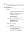
This chapter describes all functions available in the menu ‘File’ as shown in Figure 4.6.
Figure 4.6:
The menu ‘File’.
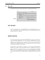
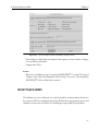
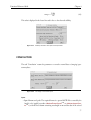
SHOW TEXTFILE
This tool is a convenient way to browse any ASCII file on the current working directory (e.g.
to look at an ENVI Header or at some ASCII auxiliary data). The file is displayed directly in
the MODO main window and may be updated through the button ‘Reload Text File’ at the
button of the window. This tool is convenient to monitor the development of a MODT42
Functions Reference Guide
Chapter 4
RAN®-5 runor for debugging purposes of faulty tape5s (display tape6 for that purpose). See
detailed description about text editing in Section 4.1.3 on Page 36.
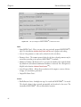
DISPLAY ENVI FILE
This is a standard method to display ENVI files, limited to files stored in band sequential
(BSQ) storage order. Clicking in the zoom window allows to display the spectra and to export
them to an ASCII file.
Figure 4.7:
Display ENVI File.
43
Chapter 4
Functions Reference Guide
QUICK PLOT
This function allows you to plot any tabular ASCII file with the MODO standard plotting
function. See detailed description about plotting in Section 4.1.6 on Page 40.
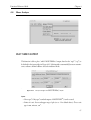
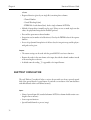
PLOT RESPONSE FUNCTION
By entering inputs as described below, the ‘Sensor Response Viewer’ (see Figure 4.8), allows
you to plot a sensors response function curves with the MODO standard plotting function
described in Section 4.1.6 on Page 40.
Figure 4.8:
The widget ‘Sensor Response Viewer’.
Inputs
• Select Sensors Response: Standard response files (‘.rsp’ or ‘.spc’) can be selected. By default,
the MODO response functions collection is provided.
‘.rsp’: one file per band, explicite response, files are selected automatically in a sequence
‘.spc’: one file per sensor, gaussian response assumption
• Channels/Bands: Enter first and last band of channel range to be plotted.
• Normalization of Response: Normalize the response to their area or to their maximum
(during convolution, the normalization does not influcence the results).
Actions
• Plot: Plots the selected response function curves
44
Functions Reference Guide
Chapter 4
SAVE STATUS
This function allows to save the current status of the internal MODO variables to a status file
(which is an IDL binary dump). This may be useful for later recovery and documentation of
your workflow procedure.
RESTORE STATUS
This brings you back to an earlier status of processing by restoring a MODO status file.
Attention: Only metadata such as file names and some of the settings are restored - MODO
does not keep track of the full situation.
STOP
If MODO is started from a full IDL installation, this function allows to stop its execution and
brings you back to the IDL prompt. All internal variables are available at this stage and it would
be possible to access them and change them within IDL (use the IDL help function for an overview of the available variables).
See detailed description about batch processing in Section 4.9 on Page 84.
RESET SESSION
If for any reason the session gets confused, this function helps to clean up strange settings.
45
Chapter 4
Functions Reference Guide
DELETE TAPE
This function allows you to conveniently delete unneeded tapes together with all related outputs. If any of the outputs is selected, only output files are deleted whereas the tape5 is retained.
SHOW SYSTEM FILE
This function allows to display an ASCII file from within the MODO installation. Use this
function to have a quick look at , e.g., a solar reference file or to a sensor response.
46
Functions Reference Guide
4.3
Chapter 4
Menu: Edit
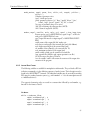
The menu ‘Edit’ contains some basic functionalities to deal with spectral data files.
Figure4.9:T
h
EDIT TEXTFILE
This tool is a convenient way to edit any ASCII file on the current working directory (e.g. to
look at an ENVI Header or at some ASCII auxiliary data). See detailed description about text
editing in Section 4.1.3 on Page 36.
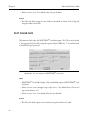
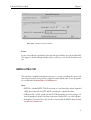
IMPORT SPECTRA
This routine is used to import spectral data to MODTRAN®-5. Two types of external data are
supported: ENVI spectral library files (‘.sli’ /’.slb’) and columnar ASCII files (labels on top, first
column contains wavelength reference in nm/microns). The procedure automatically detects
which filetype is provided. It also looks for the wavelength reference and converts to microns
if nanometers are provided in the first column.
The destination of the file (default: ‘spec_alb.dat’) can be freely chosen although MODTRAN®-5 only considers the file in the ‘DATA’ directory in standard mode, as shown in
Figure 4.10. You have to replace this file if you want to use the imported spectra in MODTRAN®-5 without using MODO afterwards. Exception: when the 'LAMBER' option of CARD
1 is chosen, the name of the spectral albedo file can be explicitely given and is stored in card
4L1.
47
Chapter 4
Functions Reference Guide
Figure 4.10:
The widget ‘Import Reflectance Spectra’.
Actions
• Select Spectra: if your input file consists of more than one spectrum, this function allows
you to pick individual spectra to import as shown in Figure 4.11.
• Import Spectra: Converts the external data to the ‘spec_alb.dat’ - like MODTRAN®-5
input file.
Figure 4.11:
48
The widget ‘Select Spectra’.
Functions Reference Guide
Chapter 4
EXPORT SPECTRA
This routine is used to export spectral data to a spectral library. An ENVI spectral library file
(‘.sli’/’.slb’) can be created out of columnar ASCII file (labels on top, first column contains
wavelength reference in nm/microns). The procedure automatically detects which filetype is
provided. It also looks for the wavelength reference and converts to microns if nanometers are
provided in the first column.
Actions
• Select: Selects ASCII spectral data (columnar file).
• Define: Defines name of output spectral library.
• Export: Creates a spectral library out of the ASCII data.
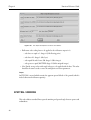
LABELS AND COLUMNS
Use this task to delete columns of spectral files and change the naming of the columns.
Figure 4.12 shows how the column named ‘Value’ is renamed by setting the column number
to ‘2’ and entering the new column name in the field ‘Label value’. Choose ‘Delete Column’
to delete the respective column.
Figure 4.12:
Editing spectral files with the function ‘Edit Column Labels or Delete Columns’.
Outputs
49
Chapter 4
Functions Reference Guide
• A file of the same reference containing this in the first column and the values in the following columns is returned.
Restrictions
• The selected input file should be of spectral ASCII format (one title-row with the labels),
first column reference.
• Don't use more than 11 characters per column name (at least two spaces should be left
between two names).
50
Functions Reference Guide
4.4
Chapter 4
Menu MODTRAN®-5: Setting up a tape5
This central part is described in more detail as the tape5 translator is a somewhat tricky but
powerful tool to work with. The sub-menus are explained in order of appearance afterwards.
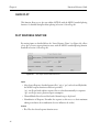
SETUP TAPE5 AND RUN
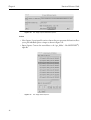
When beginning to set up or run a tape5, you are first asked to give an old tape5 to be read in.
Choose a user-defined file or one of the predefined files from the folders ‘bin’ or ‘demo_data’.
The demo files are described in Section 2.5.2 on Page 21.
Next, the MODTRAN®-5 base widget (part of the user interface 'MODO') shown in
Figure 4.13 pops up. The parameters are listed in the same order as in the tape5, each main
CARD (1-5) is surrounded by a frame. The coded values of tape5 are mostly decoded in single
pulldown menus or may be given in numeric fields. Just go through and do the used switches.
Actions
• Help: Opens a new window to display a help file with almost the same content as given in
this chapter. Consider the >Help:Browse Manual< function described in Section 4.1.2 on
Page 36, if you have a browsable manual installed.
• Select: Selects another existing tape5 and displays the contents of the last run in the widgets.
• Show Current: Shows the ASCII-encoded tape5-version of the current contents of the
widget, as it would be saved and used by MODTRAN.
• Save: Saves the current tape5 under the filename it was opened and at the position of the
current tape. Save your CARDs prior to run MODTRAN®-5 to make sure all setting have
been taken.
• Save As: Saves the current tape5 and makes a copy to a new filename.
• Clone: Saves the current run to a new filename (forgets the other runs of the same tape5).
• '>>': Switches to the next MODTRAN®-5 run in multiple run files or appends the current
tape5 at the end of the previously saved file. Allows to create multiple MODTRAN®-5
runs. CARD 5 values are created automatically.
• '<<': Switches to the previous MODTRAN®-5 run in multiple run tape5.
51
Chapter 4
Functions Reference Guide
Figure 4.13:
The widget ‘Editing Tape5 for
MODTRAN®-5’.
• Kill: Kills the current tape5 out of multiple run files.
• Run MODTRAN: Runs MODTRAN®-5 version 4, using the command 'modtran' and
assuming the MODTRAN®-5 run-script being installed.
• DONE: Quits the tape5 generator.
The following cases can not be handled with this version of the tape5-generator. For all these
purposes, you must still use a text editor or another input programm to change the tape5 and
run MODTRAN®-5 afterwards.
Restrictions
• CARD 2C1 for user given atmospheric profiles can not be easily generated, but can be
52
Functions Reference Guide
Chapter 4
changed using the 'set profile' function.
• CARD 2C2 for additional trace gas profiles can not be changed and viewed.
• CARD 2D for user given aerosol profiles can not be changed and viewed and is not supported by the interface.
• CARD 2E for user defined cloud parameters is not supported.
• The novam and the USS aerosol algortithms are not supported.
• It is not possible to edit user-defined aerosol phase functions (CARD 3B1, 3B2, 3C13C6).
• Support for BRDF models is not yet given (CARD 4B1-4B3).
Special features and hints
• Self defined background reflectance spectra can be defined in the file named 'spec_alb.dat'
in the ‘DATA’ directory, use them with ‘-[number]’ in the ‘Albedo’ field. Alternatively,
you may choose the ‘>Spectr<‘ or the ‘>LAMBER<‘ option from the dropdown menu
‘Albedo’, as described in Section 4.1.4 on Page 37 and Section 4.1.5 on Page 38, respectively.
• Switches, which require additional, non implemented CARDs are bracketed by ‘[>xx<]’,
whereas implemented features are given as ‘>xx<‘.
• Own atmospheres can be defined using the 'Define' button.
• The x-unit switch directly calculates appropriate ranges in CARD 4. All units different
from cm-1 will cause a convolved tape7-sc output. It is recommended to calculate the
results in cm-1 and use the data extraction tools afterwards for conversion to nanometers or
microns.
• Widgets are switched following the settings of individual menu points. But no logical tests
are performed - you still are allowed to make mistakes...
Input Data Format
This Section on the MODTRAN®-5 tape5 format is taken from Section 2 “Overview of Input
Data Format” of the original MODTRAN®-5 user’s manual [2]:
An attempt has been made in MODTRAN®-5 to make it easier for the users to keep track of
input and output (I/O) files. The need for easier file handling is evident to anyone who runs
MODTRAN®-5 using different tape5 input files and who wants to save the corresponding
output files (the tape6, pltout, tape7, and so on). In the past, every MODTRAN®-5 input file
had to have the name 'tape5' and previously generated I/O files had to be renamed to avoid
53
Chapter 4
Functions Reference Guide
overwriting them with newer files. The need for renaming is now avoided by creating a new
MODTRAN®-5 input file (referred to as the root name file) called either 'modroot.in' or
'MODROOT.IN'. If 'modroot.in' does not exist, MODTRAN®-5 checks for the existence of
a 'MODROOT.IN' file. If neither of these files exists, MODTRAN®-5 I/O files are the traditional ones: 'tape5', 'tape6', 'tape7', 'tape8', etc. If a root name file exists and its very first
line contains a non-null string (maximum length is 80 characters), this string is treated as a prefix. If the string consists of all blanks or is a null string, the traditional I/O file names are
assumed. The root name should contain no embedded blanks; leading and trailing blanks are
properly ignored. This string is used as a prefix for the I/O files whose names have mnemonic
suffixes. As an example, if the string is case1, the MODTRAN®-5 I/O files will have the following names:
• case1.tp5
Primary input file (tape5)
• case1.tp6
Primary output file (tape6)
• case1.tp7
Spectral plotting output file (tape7)
• case1.tp8
Auxiliary spectral data output file (tape8)
• case1.7sc
‘case1.tp7’ convolved with scanning function (tape7.scn)
• case1.7sr
Scratch file (tape7.scr)
• case1.acd
Atmospheric correction parameters
• case1.plt
Two column spectral data output file (pltout)
• case1.psc
‘case1.plt’ convolved with scanning function (pltout.scn)
• case1.clr
Spectral cooling rate data output file (clrates)
• case1.chn
Spectral data convolved with channel response functions (channels.out)
• case1.flx
Spectral diffuse and direct flux values at each atmospheric level (specflux)
MODTRAN®-5 is controlled by a single input file, 'tape5' or 'rootname.tp5', which consists
of a sequence of six or more CARDs (inputs lines). The input formats are summarized in
Table 4.1. Except when specifying file names, character inputs are case insensitive. Also,
blanks are read as zeroes for numerical inputs, and as default values otherwise. Please check the
MODTRAN®-5 manual for a detailed description of these parameters.
54
Functions Reference Guide
Table 4.1:
Chapter 4
Listing of CARDs and their format. Optional cards are marked with *.
CARD
Input Line(s)
Format
CARD 1
MODTRN, SPEED, MODEL, ITYPE, IEMSCT, IMULT, M1, M2, M3, M4,
M5, M6, MDEF, IM, NOPRNT, TPTEMP, SURREF
FORMAT (2A1, I3, 12I5, F8.3, A7)
CARD 1A
DIS, DISAZM, NSTR, LSUN, ISUN, CO2MX, H2OSTR, O3STR, LSUNFL,
LBMNAM, LFLTNM, H2OAER, SOLCON
FORMAT (2L1, I3, L1, I4, F10.5, 2A10, 4(1X, A1), 2X, F10.3)
*CARD 1A1
SUNFL2
FORMAT (A80) (If LSUNFL = True)
*CARD 1A2
BMNAME
FORMAT (A80) (If LBMNAM = True)
*CARD 1A3
FILTNM
FORMAT (A80) (If LFLTNM = True)
CARD 2
APLUS, IHAZE, CNOVAM, ISEASN, ARUSS, IVULCN, ICSTL, ICLD,
IVSA, VIS, WSS, WHH, RAINRT, GNDALT
FORMAT (A2, I3, A1, I4, A3, I2, 3I5, 5F10.5)
*CARD 2A+
ZAER11, ZAER12, SCALE1, ZAER21, ZAER22, SCALE2, ZAER31,
ZAER32, SCALE3, ZAER41, ZAER42, SCALE4
FORMAT ((3(1X, F9.0), 20X, 3(1X, F9.0))) (If APLUS = 'A+')
*CARD 2A
CTHIK, CALT, CEXT
FORMAT (3F8.3) (If ICLD = 18 or 19)
*Alternate
CARD 2A
CTHIK, CALT, CEXT, NCRALT, NCRSPC, CWAVLN, CCOLWD, CCOLIP,
CHUMID, ASYMWD, ASYMIP
FORMAT (3F8.3, 2I4, 6F8.3) (If ICLD = 1-10)
*CARD 2B
ZCVSA, ZTVSA, ZINVSA
FORMAT (3F10.3) (If IVSA = 1)
*CARD 2C
ML, IRD1, IRD2, TITLE
FORMAT (3I5, A65) (If MODEL = 0 or 7, and IM = 1)
*CARD 2C11
ZM, P, T, WMOL(1), WMOL(2), WMOL(3), (JCHAR(J), J = 1, 14),
JCHARX
FORMAT (F10.3, 5E10.3, 14A1, 1X, A1)
*CARD 2C21
(WMOL(J), J = 4, 12)
FORMAT (8E10.3, /E10.3) (If IRD1 = 1)
*CARD 2C2X1
(WMOLX(J), J = 1, 13)
FORMAT (8E10.3, /5E10.3) (If MDEF = 2 & IRD1 = 1)
*CARD 2C31
AHAZE, EQLWCZ, RRATZ, IHA1, ICLD1, IVUL1, ISEA1, ICHR1
FORMAT (10X, 3F10.3, 5I5) (If IRD2 = 1)
*CARD 2D
(IREG(N), N = 1, 2, 3, 4)
FORMAT (4I5) (If IHAZE = 7 or ICLD = 11)
55
Chapter 4
Functions Reference Guide
Table 4.1:
56
Listing of CARDs and their format. Optional cards are marked with *.
CARD
Input Line(s)
Format
*CARD 2D1
AWCCON, TITLE
FORMAT (E10.3, A70)
*CARD 2D22
(VX(N, I), EXTC(N, I), ABSC(N, I), ASYM(N, I), I = l, 2, ..., Imax)
FORMAT ((3(F6.2, 2F7.5, F6.4)))
*CARD 2E1
(ZCLD(I, 0), CLD(I, 0), CLDICE(I, 0), RR(I, 0), I = 1, NCRALT)
FORMAT((4F10.5)) (If ICLD = 1 - 10, NCRALT > 2)
*CARD 2E2
(WAVLEN(I), EXTC(6, I), ABSC(6, I), ASYM(6, I), EXTC(7, I), ABSC(7,
I), ASYM(7, I), I = 1, NCRSPC)
FORMAT((7F10.5)) (If ICLD = 1 - 10, NCRSPC > 1)
CARD 3
H1, H2, ANGLE, RANGE, BETA, RO, LENN, PHI
FORMAT (6F10.3, I5, 5X, F10.3)
Alternate
CARD 3
H1, H2, ANGLE, IDAY, RO, ISOURC, ANGLEM
FORMAT (3F10.3, I5, 5X, F10.3, I5, F10.3) (If IEMSCT = 3)
*CARD 3A1
IPARM, IPH, IDAY, ISOUR
FORMAT (4I5) (If IEMSCT = 2)
*CARD 3A2
PARM1, PARM2, PARM3, PARM4, TIME, PSIPO, ANGLEM, G
FORMAT (8F10.3) (If IEMSCT = 2)
*CARD 3B1
NANGLS, NWLF
FORMAT (2I5) (If IPH = 1)
*CARD 3B2
(ANGF(I), F(1, I, 1), F(2, I, 1), F(3, I, 1), F(4, I, 1), I = l, NANGLS)
FORMAT (8(1X, F9.0)) (If IPH = 1 and NWLF = 0)
*CARD 3C1
(ANGF(I), I = 1, NANGLS)
FORMAT (8(1X, F9.0)) (If IPH = 1 and NWLF > 0)
*CARD 3C2
(WLF(J), J = 1, NWLF)
FORMAT (8(1X, F9.0)) (If IPH = 1 and NWLF > 0)
*CARD 3C33
(F(1, I, J), J = 1, NWLF)
FORMAT (8(1X, E9.3)) (If IPH = 1 and NWLF > 0)
*CARD 3C43
(F(2, I, J), J = 1, NWLF)
FORMAT (8(1X, E9.3)) (If IPH = 1 and NWLF > 0)
*CARD 3C53
(F(3, I, J), J = 1, NWLF)
FORMAT (8(1X, E9.3)) (If IPH = 1 and NWLF > 0)
*CARD 3C63
(F(4, I, J), J = 1, NWLF)
FORMAT (8(1X, E9.3)) (If IPH = 1 and NWLF > 0)
CARD 4
V1, V2, DV, FWHM, YFLAG, XFLAG, DLIMIT, FLAGS
FORMAT (4F10.0, 2A1, A8, A7)
*CARD 4A
NSURF, AATEMP
FORMAT (I1, F9.0) (If SURREF = 'BRDF' or 'LAMBER')
Functions Reference Guide
Table 4.1:
Chapter 4
Listing of CARDs and their format. Optional cards are marked with *.
CARD
Input Line(s)
Format
*CARD 4B14
CBRDF
FORMAT (A80)
4
(If SURREF = 'BRDF')
*CARD 4B2
NWVSRF, SURFZN, SURFAZ
FORMAT (*) (If SURREF = 'BRDF')
*CARD 4B34,5
WVSURF, (PARAMS(I), I = 1, NPARAM)
FORMAT (*) (If SURREF = 'BRDF')
*CARD 4L1
SALBFL
FORMAT (A80)
(If SURREF = 'LAMBER')
*CARD 4L24
CSALB
FORMAT (A80)
(If SURREF = 'LAMBER')
CARD 5
IRPT
FORMAT (I5)
1.
is repeated ML times
if ARUSS = 'USS' and IREG(N) > 1, then Imax = IREG(N); Else Imax = 47
3.
'I' is angle index as in CARD 3C1 and 'J' is the wavelength index as in CARD 3C2
4.
set of inputs is repeated NSURF times
5. is repeated NWVSRF times
2.
MODTRAN®-5 A+ OPTION
The A+ option is set in MODO’s MODTRAN®-5 base widget, by switching the atmosphere
layer button from ‘>Default<‘ to ‘>Aero<‘. It allows you to define the layer boundaries for four
atmosphere layers as shown in Figure 4.14.
Inputs
• Boundaries: Outer limits of the aerosol regions. A smooth transitions between the layers is
given within the overlapping area.
• Scaling: Factor to scale the amount of aerosols per layer (Factor of 1: Default, no scaling).
Attention: This is a modal widget - any other IDL widgets will be blocked during execution.
57
Chapter 4
Functions Reference Guide
Figure 4.14:
The widget ‘Define Aerosol Layers’ for option A+ in MODTRAN.
Actions
• Set Defaults: Sets the boundaries and scaling factors to the values as used by MODTRAN®-5 without A+ option.
• Done: The new boundaries are transferred to the tape5 editing process. You may cancel
this transfer afterwards by omitting the ‘>A-Plus<‘ option in CARD 2 of the main widget.
MODTRAN®-5 AEROSOL OPTION
The Aerosol option is set in MODO’s MODTRAN®-5 base widget, by switching the aerosol
layer button from ‘>Default<‘ to ‘>USS<‘. It allows you to define the dimensions of the USS
option as shown in Figure 4.15.
Inputs
• Title: Describe your aerosol or cloud region.
• Conversion Factor: Is a conversion factor from extinction coefficient (km-1) to equivalent
liquid water content (g/m3). It is numerically equal to the equivalent liquid water content
corresponding to an extinction coefficient of 1.0 km-1, at a wavelength of 0.55 microns.
AWCCON has units of (km g m-3).
• Number of Spectral Points: Gives the number of spectral points to be defined for the
ARUSS option.
Actions
58
Functions Reference Guide
Figure 4.15:
Chapter 4
The widget ‘Define Aerosol Layers’ for Option ARUSS in MODTRAN.
• Cancel: No changes are made to the data.
• Done: The new data is transferred to the active tape5 generator window.
Attention: This is a modal widget - any other IDL widgets will be blocked during execution.
59
Chapter 4
4.5
Functions Reference Guide
Menu: MODTRAN
The menu ‘Modtran’ contains all MODO tasks directly related to MODTRAN®-5 calculations. While most of the functions are explained one-by-one in this chapter, the handling of
tape5 files is described in detail in Section 4.4 on Page 51.
Figure 4.16:
The menu ‘MODTRAN
®-5’.
SETUP TAPE5 AND RUN
See prior Section 4.4 on Page 51.
RUN FROM TAPE5
If you have defined and saved your tape5 in >Modtran:Setup Tape5 and Run p.60< earlier, you
may want to run MODTRAN®-5 right away.
60
Functions Reference Guide
Chapter 4
AT-SENSOR SIGNAL
The widget ‘Streamlined sensor simulation through MODTRAN’ allows you to simulate a specific at-sensor radiance signal using the major remote sensing-relevant parameters.
Figure 4.17:
The
MODTRAN®-5 ‘At-Sensor Radiance Simulator’.
Inputs
• Calculation Type: Allows to select between four standard MODTRAN®-5 options. For
broadband sensors, the low resolution is accurate enough while for high sensibility the
more accurate but slower options should be taken. The respective default tape5s for the
four options can be found (and potentially edited) in the ‘/bin’ directory of the MODO
installation; files ‘sensor0.tp5’ to ‘sensor3.tp5’.
- Low Res: Uses the 15 cm-1 band model, at high speed. This results in about 10 nm
resolution at 2.5 microns,1.5 nm at 1 micron, 0.4 nm at 0.5 micron. It makes the calculation really fast.
61
Chapter 4
Functions Reference Guide
- High Res: Uses the 1cm-1 high resolution band model. It improves the resolution by
a factor of 15 and reduces the speed almost by a factor of 10.
- High Res with DISORT: Uses the 8 stream DISORT aerosol scattering algorithm
instead of the standard ISAAC algorithm.
- High Res with DISORT and C-K: Uses the correlated-k approach for gaseous absorption calculation. This results in very slow operation of MODTRAN, but highest possible accuracy.
• Atmosphere: Select the following atmospheric settings:
- Model: Defines the profile of the atmosphere (standard profiles).
- Output mode: Defines the type of output you need. The procedures always selects the
total values. For components only, please use the function >Modtran:Setup Tape5 and
Run p.60<
- Gases: Set the amount of gases. For H20 and 03, you enter either the scaling relative to
the default values in the atmospheric models (a value of 1.0 amounts for the default
values; compare Section 2.4.2) or you enter the absolute columnar amount in g cm-2
using a preceding letter ‘g’ directly followed by the value.
- Aerosol: Enter the aerosol model and the respective visibility.
• Surface: Reflectance and Temperature of the ground is entered. Selecting ‘>Spectrum<‘ or
‘>Lambert<‘ allows to select from the currently available background reflectance spectra,
as described in Section 4.1.4 on Page 37 and Section 4.1.5 on Page 38, respectively.
• Geometry: Sensor and Sun geometric parameters define the external geometric situation.
Use the angle calculator if the angles are not known.
• Sensor: Spectral response of the sensor output - the MODTRAN®-5 run is setup such that
it covers the range between the first and the last spectral band of a sensor. The output is
convolved to the selected bands after operation.
Actions
• Export Tape5: Instead of running the whole thing, the created tape5 may be stored for
future reference.
• Calculate: Makes a copy of a standard tape5 (which can be found in the ‘/bin’ directory)
changes its parameters and starts MODTRAN. Convolution is done automatically to the
extracted main column output.
Output
• Standard ASCII file
62
Functions Reference Guide
Chapter 4
ATMO-COR PARAMETERS
For a simple atmospheric correction as described in Section 3.6 on Page 32, the atmospheric
parameters need to be calculated for a specific remote sensing situation. The respective parameters are to be calculated in advance.
Figure 4.18:
Preparation of atmospheric correction parameters.
Inputs
• Calculation type: this is mainly a matter of accuracy, 15cm-1 standard calculations are usually sufficient for most optical instruments. The 1cm-1 resolution is only required for high
spectral resolution spectrometers, whereas the considerable slower Correlated-K option
improves the accuracy specifically in absorption bands
• Atmospheric model and the optional water vapor amount are mainly driving the accuracy
of the water vapor correction in the outputs whereas the aerosol model and the horizontal
visibility (or optical thickness if a negative number is given).
63
Chapter 4
Functions Reference Guide
• The geometry section allows to enter the standard geometric situation for an image scene.
Note that the simple atmospheric correction as implemented herein does not allow for
varying parameters within an image; thus, the average value per scene is to be entered here.
• As for the sensor definition, the appropriate sensor response file (series) has to be selected.
The correct number of bands is displayed automatically when the sensor is recognized.
Actions
• Export Tape5: instead of running the whole thing, the created tape5 may be stored for
future reference or to be used with other MODO modules.
• Calculate: Makes a copy of a standard tape5 (which can be found in the ‘/bin’ directory)
changes its parameters and starts MODTRAN. The relevant parameters for atmospheric
correction are then calculated and stored. Convolution is done automatically to the
extracted main column output.
Output
• An ASCII file containing the band-wavelength reference and all corresponding correction
parameters is created. It may be used with the function xxx
PARAMETER SERIES
The calculation of series is a task often used in MODTRAN, mainly for sensitivity analysis but
also for the creation of LUTs for atmospheric processing. MODO allows the automatic creation and calculation of such series on the basis of a standard tape5, which needs to be prepared
initially.
Inputs
• Input-MOD4-Tape5: Here, you may select any previously prepared MODTRAN®-5
tape5. Use the function >Modtran:Setup Tape5 and Run p.60< to prepare such a thing.
• Series of: One parameter at a time can be selected to be the series driver.
• Parameter Series: The comma-separated values for the above selected Parameter may be
entered here according to the respective MODTRAN®-5 standards.
• Number of Column: Enter the number of the required column in this field (by default the
total radiance/transmittance/irradiance is extracted). A helpful description is given in
>Modtran:Extract Spectra p.69<.
64
Functions Reference Guide
Figure 4.19:
Chapter 4
The input widget for
MODTRAN®-5 parameter series.
• Sensor Response: Allows direct convolution of the outputs to a sensor of choice - if empty,
no convolution is performed.
• Output name: Guess...
Actions:
• Run Series: A multiple-run tape5 is created and MODTRAN®-5 is started. The selected
column is then extracted automatically and convolved to the sensor. The intermediate
MODTRAN®-5 files are deleted after execution.
REFLECTANCE SERIES
The calculation of series of reflectances is a task often used for sensitivity analysis but also for
the creation of LUTs for atmospheric processing. MODO allows the automatic creation and
calculation of such series on the basis of a standard tape5 using an ENVI spectral library.
65
Chapter 4
Functions Reference Guide
Figure 4.20:
The input widget for
MODTRAN®-5 reflectance series.
Inputs
• Input-MOD4-Tape5 : Here, you may select any previously prepared MODTRAN®-5
tape5. Use the function >Modtran:Setup Tape5 and Run p.60< to prepare such a thing.
• Series of: One parameter at a time can be selected to be the series driver.
• Parameter Series: The comma-separated values for the above selected parameter may be
entered here according to the respective MODTRAN®-5 standards.
• Number of Column to Be Extracted: Let's you enter the number of the required column
(by default the total radiance/transmittance/irradiance is extracted). For a description see
help file in the function >Modtran:Extract Spectra p.69<.
• Sensor Response-File[s]: Allows direct convolution of the outputs to a sensor of choice if empty, no convolution is performed.
• Output File Name: Guess...
Actions:
• Run Reflectance Series: A multiple-run tape5 is created and MODTRAN®-5 is started.
The selected column is then extracted automatically and convolved to the sensor. The
intermediate MODTRAN®-5 files are deleted after execution.
66
Functions Reference Guide
4.6
Chapter 4
Menu: Analyze
PLOT TAPE7 OUTPUT
This function is able to plot a 'whole' MODTRAN®-5 output, based on the ‘tape7' (‘.tp7’) to
be defined in the input widget in Figure 4.21. It distinguishes automatically between transmittance, radiance, thermal radiance and solar irradiance mode.
Figure 4.21:
The input widget ‘Plot
MODTRAN®-5 Tape7’.
Inputs
• Select tape7: Only tape7 standard outputs of MODTRAN®-5 can be treated.
• Limits of x-axis: Lower and upper range of plot (set to -1 for default values). Choose axis
type in nm, microns, cm-1.
67
Chapter 4
Functions Reference Guide
• Limits of y-axis: Set to -1 for default value, else give the limits.
Actions
• Plot: Plots the whole output in a new window as described in Section 4.1.6 on Page 40,
using the rainbow color table.
PLOT SOLAR FLUX
This function is able to plot the MODTRAN®-5 solar flux output (‘.flx’). The creation of such
a ‘.flx’ output can be fostered by setting the respective flag in CARD 4 to 'T' (second last menu
in the MODO-tape5 generator).
Figure 4.22:
The input widget ‘Plot
MODTRAN®-5 Solar Flux’.
Inputs
• MODTRAN®-5 Solar Flux Output: Only standard flux outputs of MODTRAN®-5 can
be plotted.
• Limits of x-axis: Lower and upper range of plot (set to -1 for default values). Choose axis
type in nm, microns, cm-1.
• Limits of y-axis: Set to -1 for default value, else give the limits.
Actions
• Plot: Plots the whole output in a new window, using the rainbow color table.
68
Functions Reference Guide
Chapter 4
EXTRACT SPECTRA
The input file is a tape7 originating from radiance or for transmittance runs. The output file
contains only the data within the given wavelength range at maximal at the resolution as given
by the minimal resolution.
Figure 4.23:
The widget ‘Extract Data from
MODTRAN®-5 Output’.
Options
• Unit Conversion: Choose conversion if required only. If you extract your data from
tape7_sc (‘.7sc’), no conversion may be appropriate if micron or nanmometer units were
chosen in CARD 4. Never choose conversion for transmittance/optical thickness values
since they are unitless. All calculations are principally made in/to nm.
Attention: Radiance data are converted to the unit: W/(m2 sr nm), Irradiance/solar flux data are
converted to: W/(m2 nm) and all calculations are principally made in/to nm.
• Number of the column(s) to be extracted: Enter a number or extract certain columns out
of the file by listing their numbers divided by a ','. The numbers of the columns to be
extracted depend on the type of the Input-MOD4-File (see below for the numbers). Columns are numbered starting with 1.
• Extract Spectra: Extracts the selected columns from tape7 and writes them to a simple
columnar ASCII file. One file per MODTRAN®-5 run in tape7 is written.
• Extract & Append: Same as Extract, but appends the created files to one single columnar
69
Chapter 4
Functions Reference Guide
ASCII file. This requires to have the same reference wavelengths for all runs.
• Radiance Mode: for a MODTRAN®-5 tape7 created in radiance mode, the output is
slightly different wheter the ISAAC multiple scattering calculations are chosen or the DISORT algorithm. All cases are listed in Table 4.2.
Table 4.2:
Columnar format of the radiances in ISAAC and DISORT outputs
Output Unit
ISAAC
DISORT
Total Transmittance
[-]
2
2
Path Thermal Radiance
2
3
3
2
4
2
Path Thermal Scattered
W/(m sr nm)
W/(m sr nm)
Surface Emission
W/(m sr nm)
5
4
Path scattered Radiance (total)
W/(m2
sr nm)
6
5
Path scattered Radiance (singlesc.)
W/(m sr nm)
7
6
Total ground reflected Radiance
W/(m2 sr nm)
8
7
Ground reflected Radiance (direct)
W/(m2 sr nm)
Total Radiance at the Sensor
2
9
8
2
10
9
2
W/(m sr nm)
Reference Solar Radiance
W/(m sr nm)
11
10
Reference Solar at Observer
W/(m2
12
11
sr nm)
Optical Depth
[-]
13
12
Direct Emission [-]:
[-]
14
13
15
14
16
15
Top of Atmosphere Sun
BlackBody Temperature [K]
W/(m2
nm)
[K]
• Thermal Radiance: from a MODTRAN®-5 tape7 created in thermal radiance mode, 8
columns are created; they are listed in Table 4.3.
Table 4.3:
Columnar format of the thermal radiances in ISAAC and DISORT outputs
Output Unit
Total Transmittance
Path Thermal Radiance
Path Thermal Scattered
70
[-]
W/(m2
ISAAC
DISORT
2
2
3
sr nm)
3
2
W/(m sr nm)
4
2
Surface Emission
W/(m sr nm)
5
4
Total ground reflected Radiance
W/(m2
sr nm)
6
5
Total Radiance at the Sensor
W/(m2 sr nm)
7
6
Functions Reference Guide
Table 4.3:
Chapter 4
Columnar format of the thermal radiances in ISAAC and DISORT outputs
Output Unit
ISAAC
DISORT
Optical Depth
[-]
8
7
Direct Emission:
[-]
9
8
BlackBody Temperature
[K]
10
9
• Solar Irradiance: From a MODTRAN®-5 tape7 created in solar irradiance mode, the
numbers are listed in Table 4.4.
Table 4.4:
Columnar format of the solar irradiance in ISAAC and DISORT outputs
Output Unit
Total Transmittance
Transmitted Irradiance
Solar Irradiance
Optical Depth
[-]
W/(m2
Column Number
2
nm)
3
2
W/(m nm)
4
[-]
5
• Solar Flux: For the column numbers from a MODTRAN®-5 ‘.flx’ created in radiance
mode, see Table 4.5. In addition, the altitude for the irradiance can be given. The result is
then interpolated directly from the flux file. The solar flux is defined perpendicular to the
surface. Solar flux should be calculated in cm-1 units for proper extraction. Data is converted to W/(m2 nm).
Table 4.5:
Columnar format of the solar flux in ISAAC and DISORT outputs
Output Unit
Upward diffuse
Column Number
2
W/(m nm)
2
2
downward diffuse
W/(m nm)
3
downward direct
W/(m2
4
nm)
• Transmittance: from a MODTRAN®-5 tape7 created in transmittance mode, the number
of the columns to select for each trace gas are shown in Table 4.6. No further conversions
71
Chapter 4
Functions Reference Guide
have to be performed with transmittance data.
Table 4.6:
Columnar format of the thermal radiances in ISAAC and DISORT outputs
tape7 (n_col=35)
Total
2
H2O
3
UMIX
4
CO2+
O3
trace
6
N2 cont.
7
H2O cont.
8
Mol. scat.
9
Aer./Cld. Hyd.
10
HNO3
11
Aer./Cld. ab.
12
-log (Aer)
72
5
13
CO2
14
C0
15
CH4
16
N2O
17
O2
18
NH3
19
NO
20
NO2
21
SO2
22
Cloud
23
CFC11
24
CFC12
25
CFC13
26
CFC14
27
CFC22
28
CFC113
29
CFC114
29
CFC115
30
Functions Reference Guide
Chapter 4
Table 4.6:
Columnar format of the thermal radiances in ISAAC and DISORT outputs
tape7 (n_col=35)
CL0 NO2
31
HNO4
32
CHCL2F
33
CCL4
34
N2O5
35
The following elements are added if additional molecules are selected in card1 (option ‘Mol’):
OH*: 37; HF*: 38; HCl*: 39; HBr*: 40; HI*: 41; ClO*: 42; OCS*: 43; H2CO*: 44;
HOCl*: 45; N2*: 46; HCN*: 47; CH3Cl*: 48; H2O2*: 49; C2H2*: 50; C2H6*; PH3*: 51.
APPEND SPECTRA
The function ‘Append Spectra’ merges spectral files of the same wavelength reference to a single
new file. The input files are to be listed in the input widget shown in Figure 4.24.
Figure 4.24:
The input file list widget ‘Append spectral files of the same base’.
Inputs
A list of spectral ASCII files must be collected. The titles of the single columns are in the first
row of the file.
73
Chapter 4
Functions Reference Guide
Outputs
A file of the same reference (appearing in the first column of the first file) and the values of the
chosen input spectra is returned. The title description is preserved.
Restrictions
The selected input files should be columnar ASCII, with only one head row (the single headrow-labels divided by at least two blanks. All the files must have the same wavelength/channel
-reference data in the first column (with label).
74
Functions Reference Guide
4.7
Chapter 4
Menu: Calculate
The ‘Calculate’ menu offers additional functionalities as listed in Figure 4.25
Figure 4.25:
The menu ‘Calculate’
SOLAR ANGLES
To calculate solar azimuth and zenith for a given date and position on the globe, the tool
“Sunny” was provided 'as is' by the DLR Oberpfaffenhofen. A screenshot is given in
Figure 4.26.
Enter date, time as GMT, and geograhic longitude and latitude (positive values for east of
Greenwich and north of Equator), then click ‘Do Calculation’. Solar angles and day of the year
are displayed in the output lines.
75
Chapter 4
Functions Reference Guide
Figure 4.26:
Solar angle calculator with input and output fields.
METEOROLOGICAL RANGE
The function ‘Calculate Visibility’ (see Figure 4.27) estimates the meteorological range (visibility) as used with MODTRAN®-5 from vertical optical thickness using Koschmieder equation,
which is
------------range = 3.912
ext
(4.1)
where 'ext' ist the extinction coefficient at 550 nm.
By default it is assumed, that a layer of 1 km thickness is relevant for the whole vertical aerosol
load. For this case, the extinction coefficient is of the same value as the optical thickness. The
parameter aerosol layer thickness lets you enter another layer corresponding to the aerosol vertical optical thickness.
The meteorological range is related to the observed visibility (vis) through
range = 1.3 + ( – 0.3vis )
Newer WMO recommendations tend towards an updated Koschmieder constant with
76
(4.2)
Functions Reference Guide
Chapter 4
2.996
range = ------------ext
(4.3)
This value is displayed in the lowest line and is close to the observed visibility.
Figure 4.27:
Visibility calculator with input and output fields.
CONVOLUTION
The task ‘Convolution’ returns the parameters to convolve external data to (imaging) spectrometry data.
Figure 4.28:
The widget ‘Convolution Input’
Inputs
• Input filename and -path: The required format is a spectral ASCII-File as created by the
'modex' or the ‘appfal'-procedure (>Modtran:Extract Spectra p.69< or >Modtran:Append Spectra p.73<), with the first column containing wavelength in nm and the data in the second
77
Chapter 4
Functions Reference Guide
column.
• Response-Function (given by one single file) containing three columns:
- Channel Number
- Central Wavelength [nm]
- FWHM file of each channel [nm], both as single columnar ASCII-Files
• Method of interpolation (normally step by step): If there are not so much single raw data
values, the polynomial interpolation should be prefered.
• First and last spectrometer channel number
• Integration area (in number of std deviations): Given by the FWHM values of the response
function
• In case of a polynomial interpolation of the base data, the integration step and the polynomial grade can be given.
Outputs
• The current settings can be saved with the general MODO save/restore function.
• Returns the results in the same format as the input, but with the channel numbers instead
of the wavelengths as reference.
• As default name the ending '_f' is appended to the input filename.
SHIFTTEST CONVOLUTION
The task ‘Shifttest Convolution’ helps to retrieve the potential error from a spectral spectral
shift of the spectral bands of a spectrometer. It performs a convolution of the same databases
with shifted bands within a self-defined accuracy.
Inputs
• Name of spectral input file (standard columnar ASCII, first column should contain wavelength in nm or microns)
• Sensor response functions
• Spectral bands/channels to process (range)
78
Functions Reference Guide
Figure 4.29:
Chapter 4
Shifttest Convolution Window
Actions
A series of convolutions is performed on the data with spectral shifts as given in the shifts field).
The outputs for both wavelength and data value are written to a new text file for further analyses.
SIMPLE ATMO-COR
This tool allows a simplified atmospheric correction, i.e. inversion of calibrated at-sensor radiance values of a remote sensing system to (apparent) surface albedo values. It uses the parameters as calculated with Modtran:Atmo-Cor Parameters p.63.
Inputs
• ENVI File: Standard ENVI (TM) file consisting of a raw binary data in band sequential
(BSQ) data format and an ASCII *.hdr file containing the required Meta data.
• Calibration File: *.cal file as used with the ATCOR atmospheric correction package. contains the parameters c0 and c1 for linear conversion of image DN’s to at sensor radiance.
• Atmospheric Correction Data: select the file as created with the MODO function Modtran:Atmo-Cor Parameters p.63.
79
Chapter 4
Functions Reference Guide
Figure 4.30:
The Simple Atmospheric Correction Tool (SACO).
• Reflectance scale: scaling factor to be applied to the reflectance output in %:
- scale lower or equal to 1: datyp=4 (32bit floating point)
- scale lower 10 : datyp=1 (8bit, byte)
- scale equals 10 and is lower 500: datyp=2 (16bit integer)
- scale greater or equal 500 THEN datyp=12 (16bit unsigned integer)
• Solar Zenith: average solar zenith angle in degrees to be applied with the data. This value
should be the same as used to create the atmospheric correction parameters.
Output
An ENVI file is created which contains the apparent spectral albedo of the ground (which is
indeed a directional reflectance quantity).
SPECTRAL UNMIXING
This task calculates standard linear spectral unmixing and spectral angle between spectra and
endmembers.
80
Functions Reference Guide
Figure 4.31:
Chapter 4
The ‘Spectral Unmixing Tool’
Inputs
• Spectral File: Columnar ASCII file containg the data to be unmixed. First column should
be the wavelength reference, any number of columns is allowed.
• Endmember File: Columnar ASCII file containg wavelength reference and endmembers
for unmixing. It needs the same number of bands/spectral samples as the input spectral file.
• Calculation Type:
- Spectral Angle: Standard spectral angle calculation (SAM)
- Endmember Spectral Angle: Not yet fully implemented variation of SAM.
- Linear Spectral Unmixing: Standard unconstrained linear unmixing using singular
value decomposition.
- Unmixing with Shadow: Same as above but adding an artificial shadow endmember
which accounts for the brightness of a spectrum. The shadow endmember has a constant value of 1% of the maximum value of all other endmembers.
Output
An ASCII file is created with abundances/angles for each endmember. Each row of the file corresponds to one endmember. Shadow is the last endmember if this option is chosen (2nd last
row). The residual error estimate is given fo the unmixing results in the last row in units of the
original spectrum.
81
Chapter 4
Functions Reference Guide
OWN ROUTINE
If you got an own routine which should be accessible through the MODO interface, please
name it ‘xmod_routine.pro’ and make it accessible/compiled through IDL. It then will be
started through that button.
4.8
Menu: Help
The help menu provides direct access to the modo manuals and some basics.
WINDOW MANAGER
This widget displays a list of all currently opened windows:
82
Functions Reference Guide
Chapter 4
BASICS
Some basic information as contained in this manual is displayed.
BROWSE MODO MANUAL
Displays this manual (MODO_Manual.pdf) as contained in the modo installation directory.
Uses the operating system’s default application for PDF display; if none is set, no file is displayed.
BROWSE MODTRAN MANUAL
Displays the original MODTRAN®-5 manual (MODTRAN_Manual.pdf) as contained in the
modo installation directory. The manual is enhanced with hyperlinked bookmarks pointing
directly to each chapter. Uses the operating system’s default application for PDF display; if
none is set, no file is displayed.
ABOUT MODO
Displays some information about MODO and its current stage of development
LICENSE
Brings you to the licensing dialog to either enter the license key or to produce the information
required for a license key.
83
Chapter 4
4.9
Functions Reference Guide
Batch Processing
MODO principally can be used for batch processing of MODTRAN®-5 jobs. However, the
functions are not fully documented.
4.9.1 Batch Commands (for IDL)
Here are some useful functions available in the IDL programming environment after loading
the MODO program:
modo4, /norun
Starts up MODO-4 (defining variables) without getting to the GUI.
run_mod4, tape5, /select, /batch
Runs MODTRAN®-5 from within MODO using a specific tape5.
‘/select’: triggers selection of a tape5 by a dialog
‘/batch’: inhibits the display of dialog boxes
common c_genmod
loads the MODO common block
(after its definition by modo4,/norun)
run_mod4, tape5, group=group, select = select, batch = batch
writetape4, tape5 [,/append,/new,/silent,/kill
Writes the current variables to a MODTRAN®-5 tape5 file. By default,
the current tape is overwritten.
‘append’: Appends to the current tape.
‘/new’: Creates a new tape.
‘/silent’: Disables messages on screen.
‘kill=..’: Deletes a specific run of a tape.
readtape4, tape5 [,/cur, /silent]
Reads the contents of a tape5 to the MODO variables.
cur: number of tape5 run to be read.
silent: no feedback
mod4_reflseries, rfile, ofile, tape5 [, cfile=..]
Calculates a series of runs on the basis of reference surface reflectance
spectra.
‘rfile’: File containing the reflectance data (ASCII).
‘ofile’: Name of output file (ASCII).
‘tape5’: Name of initial tape5 (only reflectance will be changed).
‘cfile’: Name of sensor response if convolution is required.
84
Functions Reference Guide
Chapter 4
mod4_series, tape5, parm, list, ofile, col, otape5, [rfile=..,
cfile=..]
Calculates a parameter series.
‘tape5’; initial tape5 name
‘parm’: parameter selection: 'vis', 'ihaze’, 'model, 'h2ostr', 'o3str',
'co2mx', 'angle', 'parm1', 'parm2', 'h1', 'h2', or 'surref'.
‘list: array of parameter values to be varied
‘rfile’: File containing the reflectance data (ASCII).
‘ofile’: Name of output file (ASCII).
modex, tape7, outfile, wvlu, wvlo, col, resol [,/trs,/app,/var]
Extracts spectra out of a MODTRAN®-5 tape6 or tape7 - works also
with series of MODTRAN®-5 runs.
tape7: Input-File must be a output-tape6/7 of MODTRAN/LOWTRAN
outfile: name of the output-file (def: modex.out)
wvlu: lowest wavelength of the extracted data [nm] (def: 400nm)
wvlo: highest wavelength of the extracted data [nm]
col: number of the column[s] to be extracted (def: 12)
resol: maximum resolution of the output [nm]
anzfil: variable, which gets the number of created files
/app: appends files (default: each output spectrum is one file)
/trs: don’t convert the data to W/m2 sr.
/var: the variable ‘outfile’ will contain the contents of the output after
execution of the program.
4.9.2 Internal Data Format
The following variables are available for manipulation within modo. They are listed as IDL initialization commands as in the definition sequence of modo,/norun. Their description can be
found in the MODTRAN®-5 manual. The individual variables may be accessed from within
IDL using the standard structure syntax (e.g., cd1.model = 3 sets the atmospheric model
to ‘midlatitude winter’).
The respective formatting codes are stored in a structure fmt followed by card number, e.g.
fmt.cd1 for the format of card1.
File Names
mfile = {modtran_files,
tape5:'standard.tp5', $
tape6:'standard.tp6', $
tape7:'standard.tp7', $
tape8:'standard.tp8', $
85
Chapter 4
Functions Reference Guide
flux:'standard.flx', $
sp_alb:spec_alb, $
resp: modopath+'sensor_resp'+delim+'dummy.spc',
stape5: modopath+'etc'+delim+'sensor_0.tp5', $
atape5: modopath+'etc'+delim+'acdata_0.tp5'}
$
Parameters
par = {modo_parameters, $
wvlrange:[350d, 2550], $ ;lower and upper wavelength range
bandrange:lonarr(2), $;lower and upper band number
scale:10, $ ;; scale for atmospheric correction
calfile:'envi_in.cal', $ ;; name of calibration file for
atmospheric correction
acdfile:'acdfile.txt', $ ;; atmospheri correction data file
ienvi:'envi_in.bsq', $ ;; last ENVI input file called
oenvi:'envi_out.bsq', $ ;; last ENVI output file called
actype:0, $ ;; type of atmospheric correction
zen:0d, $ ;; solar zenith angle
azi:0d, $ ;; solar azimuth angle
opts:lonarr(10), $ ;; various processing options
aux1: '', $
aux2: ''}
Card 1
cd1 = {CARD1, modtrn:'T', speed:'M', binary:'F', lymolc:' ',
model:2, itype:2, iemsct:2, imult:1,m:intarr(6), mdef:0,
i_rd2c:0, noprnt:0, tptemp:293.15, surref:'0.4'}
cd1a = {CARD1A, dis:'F',disazm:'F', disalb:' ', nstr:8, sfwhm:0.,
co2mx:365.0, h2ostr:' ', o3str:' ', c_prof:0, lsunfl:'F',
lbmnam:'F', lfltnm:'F', h2oaer:'t', cdtdir:'F', solcon:0.,
cdastm:' ', astmc:0., astmx:0., astmo:0., aerrh:0.,
nssalb:0}
cd1a1 = '' & cd1a2 = '' & cd1a3 = '' &cd1a4 = ''
cd1a5 = dblarr(10)
cd1a6 = dblarr(13)
cd1a7 = dblarr(16)
Card 2
cd2
= {CARD2, aplus:'', ihaze:1, cnovam:'',iseasn:0, aruss:'',
ivulcn:1, icstl:3, icld:0, ivsa:0, vis:0.0, wss:0.0,
whh:0.0, rainrt:0.0, gndalt:0.0}
cd2ap = [0.0, 3, 1,
2, 11, 1, 10, 35, 1, 30, 100, 1]
86
Functions Reference Guide
Chapter 4
cd2a = {CARD2A, cthik:-9., calt:-9., cext:-9., ncralt:-9, ncrspc:9, cwavln:-9, ccolwd: -9, ccolip:-9, chumid:-9,asymwd:-9,
asymip:-9}
cd2b = {CARD2B, zcvsa:0., ztvsa:0., zinvsa:0.}
cd2c = {CARD2C, ml:0, ird1:0, ird2:0, hmodel:'', ree:0.0,
nmolyc:0, e_mass:0., airmwt:0.}
cd2cy = strarr(20) & cd2c1=fltarr(6,50)
cd2c1a = strarr(16, 50) ;; jchars
cd2c2= fltarr(9,50)
cd2c2x = fltarr(13, 50)
cd2c2y = fltarr(8, 50) ;; variable size according to nmolyc
cd2c3 = fltarr(8,50)
cd2d = intarr(4) + 47
cd2d1 =replicate({CARD2D1, awccon:0.0, title:''}, 4)
cd2d1.title = ['Aerosol Layer 1', 'Aerosol Layer 2',
'Aerosol Layer 3', 'Aerosol Layer 4']
cd2d2 =replicate({CARD2D2, varspc:0.0, extc:0.0, absc:0.0,
asym:0.0}, 4, 200)
cd2e1 = dblarr(4, 50) & cd2e2 = dblarr(7, 50)
cd2e2a = {CARD2E2_alt, cfile:'', cldtyp:'', cirtyp:''}
Card 3
cd3 = {CARD3_gen, h1:100.0, h2:0.0, angle:180.0}
cd3_ = {CARD3_gen2, range:0., beta:0., r0:0., lenn:0., phi:0.}
cd3alt = {CARD3_alt, iday:0, r0:0., isourc:0, anglem:0.}
cd3a1 = {CARD3A1, iparm:1.0, iph:2.0, iday:180, isourc:0}
cd3a2 = {CARD3A2, parm1:47.2, parm2:351.5, parm3:0., parm4:0.,
time:12.0, psipo:0., anglem:0., G:0.}
cd3b1 = {CARD3B1, nangls:0}
cd3b2 = fltarr(5,50)
Card 4
cd4 = {card4, v1:4000d, v2:25000d, dv:15d, fwhm:20d, yflag:' ',
xflag:'W', dlimit:'- next -', flags:' AA
'}
cd4a = {card4a, nsurf:1, aatemp:-1., dh2o:0., mltrfl:'F'}
cd4b = replicate({card4b, cbrdf:'', nwvsrf:0.0, surfzn:0.0,
surfaz:0.0}, 2)
cd4b3 = fltarr(6, 3000, 2)
cd4l = {card4l, salbfl:mfile.spec_alb, csalb1:'3', csalb2:'3'}
cd5
= 0
87
Chapter 4
88
Functions Reference Guide
MODO 4
References
References
[1]
[2]
[3]
[4]
[5]
[6]
[7]
[8]
[9]
[10]
[11]
[12]
[13]
Anderson, G.P. and Hall, L.A., 1998. Solar irradiance between 2000-3100 Angstroms with spectral
band pass of 1 Angstroms, J. Geophys. Res., 94D, 6435-6441.
Berk A., Bernsten L.S., and Robertson D.C., 1989: MODTRAN: A Moderate Resolution Model for
LOWTRAN7. Air Force Geophysics Laboratory, Hanscom AFB, MA, GL-TR-89-0122, pp.
38.
Berk, A., Bernstein, L.S., Anderson, G.P., Acharya, P.K., Robertson, D.C.,Chetwynd, J.H., and AdlerGolden, S.M., 1998: MODTRAN4 cloud and multiple scattering upgrades with application
to AVIRIS, Remote Sens. Environ., 65:367-375.
Börner A., Schaepman M., Schläpfer D., Wiest L., and Reulke R., 1999: The Simulation of APEX Data: The SENSOR approach. Imaging Spectrometry V, Denver, SPIE Vol. 3753:235-246.
Cao, C., Blonsky, S., Ryan, R. and Gasser, J., 1999. Synthetic Scene Generation of the Stennis V & V
Target Range for the Calibration of Remote Sensing Systems. ISSR.
Cebula, R., Thuillier, G., Vanhousier, R.M., Hilsenrath, E., Herse, M. and Simon, P.C., 1996. Observation of the solar irradiance in the 200-350 nm interval during the ATLAS 1 mission_ A
comparison of three sets of measurements - SSBUV, SOLSPEC and SUSIM, Geophys. Res.
Lett., 23, 2289.
Chance, K. and Spurr, R.J.D., 1997. Ring effect studies: Rayleigh Scattering, including molecular parameters for rotational raman scattering, and the Fraunhofer Spectrum, Applied Optics 36, pp.
5224-5230.
Cooley T.W., Anderson G., Felde G.W., Hoke M.L., Ratkowski A.J., Chetwynd J.H., Gardner J.A.,
Adler-Golden S.M., Matthew M.W., Berk A., Bernstein L.S., Acharya P.K., Miller D. and
Lewis P., 2002: FLAASH, A MODTRAN4-Based Atmospheric Correction Algorithm: Its Application And Validation, Proc. IGARSS 2002. IEEE, Toronto, CA, Vol. Vol. III, pp. 14141418.
Edlen, K., 1966. The Refractive Index of Air. Metrologia, 2: 12.
ENVI, 2001: The Environment for Visualizing Images, Version 3.4. Research Systems, Inc., Boulder,
Colorado, USA.
Gao, B.-C. and Green, R.O., 1995. Presence of Terrestrial Atmospheric Gas Absorption Bands in
Standard Extraterrestrial Solar Irradiance Curves in the Near-Infrared Spectral Region. Applied Optics, Vol. 34, No. 27: pp 6263 - 6268.
Halthore, R.N. et al., 1997. Comparison of model estimated and measured direct-normal solar irradiance. J. Geophys. Res., 102(D25): 29,991-30,002.
Hausknecht, P. and Richter, R., 1997. Comparison of helicopter-based spectral radiance measurements and theoretical calculations with MODTRAN, Alg. for Mult. and Hyp. Im. III, Orlando, pp. 253-258.
89
References
MODO 4
[14] IDL, 2001: Interactive Data Language (IDL), Version 5.4. Research Systems, Inc., Boulder, Colorado,
USA.
[15] Itten K.I., Schaepman M., De Vos L., Hermans L., Schlaepfer H., and Droz F., 1997: APEX-Airborne
Prism Experiment: ANew Concept for an Airborne Imaging Spectrometer. Proceedings of the
Third International Airborne Remote Sensing Conference and Exhibition, ERIM International Inc., Copenhagen (DK), Vol. I, pp. 181-188.
[16] Kindel, B.C., Qu, Z. and Goetz, A.F.H., 2001. Direct solar spectral irradiance and transmittance measurements from 350 to 2500 nm. Applied Optics, 40(21): 3483-3494.
[17] Kurucz, R.L. 1992. (1) Atomic and molecular data for opacity calculations; (2) Finding the missing
solar ultraviolet opacity; and (3) Remaining line opacity problems for the solar spectrum, all
three papers in Revista Mexican de Astronomia y Astrofisica, 23.
[18] Kurucz, R.L. 1995. The solar irradiance by computatioin, Proceedings of the 17th Annual Review
Conference on Atmospheric Transmission Models, edited by Anderson, G.P., Picard, R.H.,
and Chetwynd, J.H., PL/-TR-95-2060, Special Reports, No. 274, Pl. 332, Phillips Laboratory/Geophysics Directorate, MA.
[19] McElroy, C.T. (1995). A Spectroradiometer for the measurement of direct and scattered solar spectral
irradiance from on-board the NASA ER-2 high-altitude research aircraft, Geophys. Res. Lett.,
22, pp. 1361-1364.
[20] McElroy, C.T., Midwinter, C., Barton, D.V., and Hall, R.B. (1995). A comparison of J-values estimated by the composition and photodissociative flux measurement with model calculations,
Geophys. Res. Lett., 22, pp. 1365-1368.
[21] Miesch, C., Briottet, X., Kerr, Y.H. and Cabot, F., 2000. Radiative transfer solution for rugged and
heterogeneous scene observations. Applied Optics, 39(36): 6830-6846.
[22] Nicodemus et al.: Geometrical Considerations and Nomenclature for Reflectance. National Bureau of
Standards (1977) pp. 52.
[23] Nieke J., Itten K.I., Kaiser J.W., Schläpfer D., Brazile J., Debruyn W., Meuleman K., Kempeneers
P.B., Neukom A., Feusi H., Adolph P., Moser R., Schilliger T., Quickelberghe M.V., Alder J.,
Mollet D., Vos L.D., Kohler P., Meng M., Piesbergen J., Strobl P., Schaepman M.E., Gavira
J., Ulbrich G.J. and Meynart R., 2004: APEX: Current Status of the Airborne Dispersive Pushbroom Imaging Spectrometer. W. L. Barnes and J. J. Butler (Editors), Earth Observing Systems IX. Proc. SPIE, Vol. 5542, Maspalomas (Spain), pp. 109-116.
[24] Nieke, J. and Fukushima, H., 2002. Selection of a solar reference spectrum for GLI’s reflective bands,
preprint, pp. pp. 17.
[25] Richter R., 1997: Correction of atmospheric and topographic effects for high spatial resolution satellite
imagery. Int. J. Rem. Sens., 18(13):1099-1111.
[26] Richter R., 1998: Correction of satellite imagery over mountainous terrain. Applied Optics, Vol. 37,
No. 18: pp. 4004-4014.
[27] Richter, R., 1996. A spatially adaptive fast atmospheric correction algorithm. International Journal of
Remote Sensing, Vol. 17, No. 6: pp. 1201-1214.
[28] Richter, R., 2009: Atmospheric / Topographic Correction for Wide FOV Airborne Imagery: Model
ATCOR4. DLR Internal Report, DLR-IB 552-05/09
90
MODO 4
References
[29] Rothman, L.S. and McCann, A., 1996. HITRAN 1996.
[30] Schläpfer D. and Schaepman M., 2002: Modelling the noise equivalent radiance requirements of imaging spectrometers based on scientific applications. Applied Optics, 41(27): 5691-5701.
[31] Schläpfer D., 2001: MODO: An Interface to MODTRAN4 for the Simulation of Imaging Spectrometry At-Sensor Signals, In: 10th JPL Airborne Earth Science Workshop. JPL, Pasadena (CA),
Vol. Publication 02-1, pp. 343-350.
[32] Schläpfer D., Boerner A., and Schaepman M., 1999: The Potential of Spectral Resampling Techniques
for the Simulation of APEX Imagery based on AVIRIS Data. Summaries of the Eighth JPL Airborne Earth Science Workshop, JPL, Pasadena (CA), 99-17:377-384.
[33] Schläpfer D., Borel C.C., Keller J., and Itten K.I., 1998: Atmospheric Pre-Corrected Differential Absorption Techniques to Retrieve Columnar Water Vapor. Remote Sens. Environ., Elsevier,
65(3):353-366.
[34] Schläpfer, D., 2001. MODO: An Interface to MODTRAN4 for the Simulation of Imaging Spectrometry At-Sensor Signals, 10th JPL Airborne Earth Science Workshop. JPL, Pasadena (CA), pp.
343-350.
[35] Schmid, B. et al., 1995. Validation of Atmospheric Transmittance Models in the 0.94 Micron Region
for Sunphotometric Determination of Columnar Water Vapor. Journal of Geophysical Research: p 45.
[36] Secker, J., Staenz, K., Budkewitsch, P. and Neville, R.A., 1999. A Vicarious Calibration of the
PROBE-1 Hyperspectral Sensor, 4th Int. Airb. R. S. Conf. and Exh. ERIM, Ottawa, CA, pp.
75-82.
[37] Staenz K., Secker J., Gao B.-C., Davis C. and Nadeau C., 2002: Radiative transfer codes applied to
hyperspectral data for the retrieval of surface reflectance. ISPRS Journal of Photogrammetry
and Remote Sensing, 57(3): 194-203.
[38] Strobl P., Mueller A., Schlaepfer D., and Schaepman M., 1997: Laboratory Calibration and Inflight
Validation of the Digital Airborne Imaging Spectrometer DAIS 7915 for the 1996 Flight Season.Proceedings of SPIE AeroSense'97, Orlando, FL, p 8.
[39] Thuillier, G., Herse, M., Simon, P.C., Labs, D., Mandel, H., and Gillotay, D., 1996. Observation of
the visible solar spectral irradiance between 200 and 350 nm during the ATLAS I mission by
the SOLSPEC spectrometer, Sol. Phys., 171, pp. 283-302.
[40] Thuillier, G., Herse, M., Simon, P.C., Labs, D., Mandel, H., and Gillotay, D., 1996. Observation of
the visible solar spectral irradiance between 350 and 850 nm during the ATLAS I mission by
the SOLSPEC spectrometer, Sol. Phys., 177, pp. 41-61.
[41] Vermote, E, El Saleous, N, Justice, C O, Kaufman, Y J, Privette, J L, Remer, L, Roger, J C, Tanré:
Atmospheric correction of visible to middle-infrared EOS-MODIS data over land surfaces:
Background, operational algorithm and validation. Journal of Geophysical Research (1997)
vol. 102 (D14) pp. 17131-17141.
[42] Wang, J., Anderson, G.P., Revercomb, H.E. and Knuteson, R.O., 1996. Validation of FASCOD3 and
MODTRAN3: comparison of model calculations with ground-based and airborne interferometer observations under clear-sky conditions. Applied Optics, Vol. 35, No. 30: pp. 6028-6040.
[43] Woods, T.N., Prinz, D.K., Rottman, G.J., London, J., Crane, P.C., Cebula, R.P., Hilsenrath, E.,
91
Chapter
Brueckner, G.E., Andrews, M.D., White, O.R., VanHoosier, M.E., Floyd, L.E., Herring,
L.C., Knapp, B.G., Pankratz, C.K., Reiser, P.A. (1996). Validation of the UARS solar ultravialet irradiances: Comparison with the ATLAS 1 and 2 measurements, J. Geophys. Res., 101D,
pp. 9841-9569.
92
Index
Index
A
A+ option, 55, 57, 58
Absorption
Calculation, 62
Feature, 27, 32
Accuracy, 27, 62, 78
Adjacency effects, 6, 12, 39
Aerosol
Algorithm, 53, 62
Layer, 11, 57, 58, 76
MISR aerosol model, 7
Model, 30, 62
MODTRAN option, 58
Optical thickness, 30, 76
Phase function, 7, 53
Profile, 53
Air Force Geophysics Laboratory (AFGL), 11
Airborne Prism Experiment (APEX), 26, 32
Append spectra, 25, 69, 73
ARUSS, 55, 57, 58, 59
ATCOR, 21, 29
Atmospheric profile, 52, 62
At-sensor radiance, 7, 12, 13, 23, 24, 25, 26, 27, 28,
29, 31, 61
Auxiliary data, 36, 42, 47, 54
AVIRIS, 17, 26
B
Band model, 11, 15, 16, 61
Batch processing, 45, 84
BRDF, 7, 53, 56, 57
C
Calculate menu, 75
Convolution, 77
Meteorological range, 76
Own routine, 82
Shifttest convolution, 78
Solar angles, 75
Spectral unmixing, 80
CARD, 51, 53, 54, 55, 56, 57
CARD 1, 15, 47
CARD 1A, 16, 17
CARD 1A1, 16
CARD 1A2, 16
CARD 1A3, 17
CARD 2, 58
CARD 2C1, 52
CARD 2C2, 53
CARD 2D, 53
CARD 2E, 53
CARD 3B1, 53
CARD 3B2, 53
CARD 3C1, 53
CARD 4, 53, 68, 69
CARD 4B1, 53
CARD 4L1, 18
CARD 4L2, 18
CARD 5, 51
Cebula plus Chance database, 17
Central wavelength, 78
Chance database, 17
Cloud option, 27
Commands, 84
Computing time, 27, 61
Convolution, 5, 6, 12, 13, 14, 25, 27, 32, 44, 54, 62,
64, 65, 66, 77, 78, 84
Correlated-k, 15, 16, 27, 28, 62
D
Data Format, 85
Delta radiance simulation, 31
Demo data, 15, 21, 51
atcor_lib.sli, 21
flux.tp5, 22
irradiance.tp5, 22
radiance.tp5, 22
radiosonde.tp5, 22
radiosonde_trans.tp5, 22
sensor0.tp5, 22
sensor1.tp5, 22
93
Index
sensor2.tp5, 22
sensor3.tp5, 22
spectra_6s.txt, 21
spectral.tp5, 22
DISORT, 24, 62, 70, 71, 72
E
Edit menu, 47
Export spectra, 49
Import spectra, 47
Labels and columns, 49
Endmember, 80, 81
ENVI, 6, 9, 12, 13, 25, 36, 42, 47, 49, 65
Evaluation license, 9
Extinction coefficient, 58, 76
F
File
Display ENVI file, 43
File format, 15, 17, 37, 39
File menu, 42
Edit textfile, 47
Plot response function, 44
Quick plot, 44
Reset session, 45
Restore status, 45
Save status, 45
Show system file, 46
Show textfile, 42
Stop, 45
FORTRAN, 11
Full width half maximum (FWHM), 31, 56, 78
G
Gaussian approximation, 6, 12, 14, 25, 44
Geometry, 11, 24, 27, 29, 30, 62
Graphical user interface (GUI), 5, 6, 23, 30, 84
H
Help
About MODO, 83
Basics, 83
Browse MODO Manual, 83
License, 83
MODTRAN manual, 24, 36
Window Manager, 82
Help menu, 36
Licensing, 9
94
Tape5, 51
I
IDL, 11
Modal widget, 38, 40, 57, 59
MODO status, 45
MODO variables, 45
Own routine, 7, 82
System requirements, 8
Virtual Machine, 8, 23
Installation
IDL, 45
MODO, 8, 15, 46
Interpolation, 78
Polynomial, 78
Step by step, 78
Inversion, 25
Irradiance, 11, 16, 22, 27, 71
MODTRAN mode, 24, 67, 71
Source options, 11
Units, 17, 69
ISAAC, 62, 70, 71, 72
K
Koschmieder
Constant, 76
Equation, 76
Kurucz database, 17
L
LANDSAT7, 17
Linear spectral unmixing, 80, 81
Liquid water content, 58
Look-up-table (LUT), 25, 29, 64, 65
LOWTRAN, 15
M
Main menu, 35
Calculate, 75
Edit, 47
File, 42
MODTRAN4, 60
MISR aerosol model, 7
mod4_reflseries, 84
mod4_series, 85
modex, 85
modo.sav, 23
modo4, 84
Index
modroot.in, 54
MODTRAN
Band model, 16, 61
Base widget, 51
Data basis, 15
Manual, 36, 53
Program code, 11, 13
Simulation modes, 61
Units, 13
MODTRAN4 menu, 51, 60
Append spectra, 73
At-sensor signal, 61
Extract spectra, 69
Parameter series, 64
Plot solar flux, 68
Plot tape7 output, 67
Reflectance series, 65
Run from tape5, 60
Setup tape5 and run, 51
Multiple scattering, 29
N
Novam, 53
O
of, 24
Optical thickness, 30, 69, 76
Ozone, 62
P
Parameter series, 30, 64
Path scattered radiance, 13, 30, 70
Plot, 40
Response Function, 44
Solar flux, 68
tape7, 54, 67
Polynomial interpolation, 78
R
Radiance
At-sensor, 7, 12, 13, 23, 25, 27, 29, 31, 61
Direct reflected, 30
Extraction, 6
MODTRAN mode, 24, 67, 70
Noise equivalent, 31
Output format, 19
Path scattered, 13, 30
Per wavelength, 14
Per wavenumber, 14
Simulation, 27, 29
Thermal, 24
Units, 14, 69
Radiosonde
Profiles, 7
radiosonde.tp5, 22
readtape4, 84
Reflectance, 39, 66, 84, 85
Background, 39, 53, 62
Import, 24, 48
Output format, 19
Series, 65
spec_alb.dat, 18, 39
Remote Sensing Laboratories (RSL), 5
ReSe Applications Schläpfer, 5
Resolution, 27
Band model, 15, 16, 24, 61
Sensor, 14, 15, 31
Response function, 14, 17, 25, 32, 54, 78
Plot, 44
run_mod4, 84
S
S6, 21
Sampling interval, 31
Sensititivity analysis series, 30
Sensitivity analysis series, 64, 65
SENSOR, 32
Sensor, 62
Altitude, 29, 30
Evaluation, 31
Response function, 17, 24, 27, 44, 62, 65, 66
Response library, 31
Response viewer, 44
sensor0.tp5, 22
sensor1.tp5, 22
sensor2.tp5, 22
sensor3.tp5, 22
Simulation, 31, 61
Viewing angle, 29, 62
Shadow endmember, 81
Shifttest convolution, 78
Simulation series, 25
Solar angle, 6, 12, 29, 62, 75
Solar database, 16
Cebula plus Chance, 17
Chance, 17
95
Index
Kurucz, 17
Thuillier plus Kurrucz, 17
Solar flux, 11
Extraction, 6
flux.tp5, 22
MODTRAN mode, 71
Plotting, 12, 25, 68
Units, 69
spec_alb.dat, 11, 18, 21, 37
Spectral
Albedo, 18, 37, 38
Channel shift, 25, 78
Cooling rate, 54
Library, 6, 12, 13, 21, 25, 30, 47, 49, 65
Points, 58
Range, 22
Resolution, 15, 16, 31
Response, 15, 32, 62
Sampling, 31
Spectral Angle Mapper (SAM), 80, 81
Units, 17
Unmixing, 80, 81
Suffix, 54
Sunny, 75
System requirements, 8
T
tape5, 11, 21, 54
Editor window, 23
Multiple run, 24, 51
Parameter series, 65
Reflectance series, 65, 66
Setup and run, 51
tape6, 18
96
tape7, 18
Extract spectra, 69
Irradiance, 71
Plotting, 12, 67
Radiance mode, 70
Thermal radiance mode, 70
Transmittance mode, 71
tape8, 18
Thermal radiance
MODTRAN mode, 24, 67, 70
Thuillier plus Kurucz database, 17
Trace gas profile, 53
Transmittance, 13, 22, 29, 69
MODTRAN mode, 11, 24, 67, 71
U
Unit conversion, 13, 14, 69
Units, 13, 14, 17, 53, 58
User requests, 7
USS aerosol algortithm, 53
USS aerosol option, 58
V
variables, 85
Viewing angle, 29, 62
Visibility, 6, 29, 30, 62, 76
W
Water vapour, 62
Wavelength, 13, 14, 17, 18, 58, 78
Wavenumber, 13, 14, 17
writetape4, 84