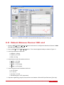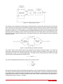
1
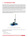
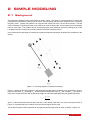
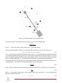
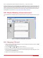
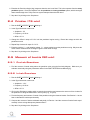
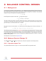
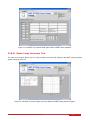
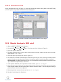
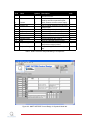
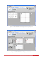
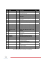
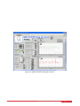
c 2011 Quanser Inc., All rights reserved.
⃝
Quanser Inc.
119 Spy Court
Markham, Ontario
L3R 5H6
Canada
[email protected]
Phone: 1-905-940-3575
Fax: 1-905-940-3576
Printed in Markham, Ontario.
For more information on the solutions Quanser Inc. offers, please visit the web site at:
http://www.quanser.com
This document and the software described in it are provided subject to a license agreement. Neither the software nor this document may be
used or copied except as specified under the terms of that license agreement. All rights are reserved and no part may be reproduced, stored in
a retrieval system or transmitted in any form or by any means, electronic, mechanical, photocopying, recording, or otherwise, without the prior
written permission of Quanser Inc.
Acknowledgements
Quanser, Inc. would like to thank the following contributors:
Dr. Hakan Gurocak, Washington State University Vancouver, USA, for his help to include embedded outcomes assessment, and
Dr. K. J. Åström, Lund University, Lund, Sweden for his immense contributions to the curriculum content.
QNET ROTPENT Laboratory Manual - Student Manual
2
Contents
1
Introduction
4
2
Simple Modeling
2.1
Background
2.2
Simple Modeling Virtual Instrument
2.3
Damping [15 min]
2.4
Friction [15 min]
2.5
Moment of Inertia [30 min]
2.6
Results
6
6
8
8
9
9
10
3
Balance Control Design
3.1
Background
3.2
Balance Control Design VI
3.3
Model Analysis [20 min]
3.4
Control Design and Simulation [45 min]
11
11
11
13
14
4
Balance Control
Implementation
4.1
Background
4.2
Balance Control VI
4.3
Default Balance Control [30 min]
4.4
Implement Designed Balance Control [20 min]
4.5
Balance Control with Friction
Compensation [30 min]
15
15
15
16
17
17
5
Swing-Up Control
5.1
Background
5.2
Swing-Up Control VI
5.3
Energy Control [30 min]
5.4
Hybrid Swing-Up Control [20 min]
19
19
21
21
22
6
System Requirements
6.1
Overview of Files
6.2
Simple Modeling Laboratory VI
6.3
Control Design VI
6.4
Swing-Up Control VI
23
23
23
24
24
7
Lab Report
7.1
Template for Content (Simple Modeling)
7.2
Template for Content (Balance Control Design)
7.3
Template for Content (Balance Control Implementation)
7.4
Template for Content (Swing-Up Control)
7.5
Tips for Report Format
30
30
31
32
33
34
QNET ROTPENT Laboratory Manual - Student Manual
v 1.0
1
INTRODUCTION
Regulation and servo problems are very common, but feedback can be used in many other useful ways. The name
task-based control is used as a common classification of a wide variety of problems. For instance, stabilization of
an unstable system can be considered a task-based problem. However, it is a borderline example since it can also
be viewed as a regulation problem. The Segway transporter is a typical example where stabilization is a key task.
In that case stabilization is also merged with the steering functions. Other examples are damping of a swinging load
on a crane, stabilization of a rocket during take-off, and the human posturing systems. There are many examples
of task-based control in aerospace such as automatic landing and orbit transfer of satellites. Robotics is a rich field
for task-based control with challenges such as collision avoidance, motion planning, and vision based control. Taskbased control is typically more complicated than regulation and servoing but they may contain servo and regulation
functions as sub-tasks. We have chosen the rotary pendulum system to illustrate task-based control
The QNET rotary inverted pendulum trainer is shown in Figure 1.1. The motor is mounted vertically in a metal
chamber. An L-shaped arm is connected to the motor shaft and pivots between ±180 degrees. A pendulum is
suspended on a horizontal axis at the end of the arm. The pendulum angle is measured by an encoder. The control
variable is the input voltage to the pulse-width modulated amplifier that drives the motor. The output variables are
the angle of the pendulum and the angle of the motor.
Figure 1.1: QNET rotary inverted pendulum trainer (ROTPENT)
There are three experiments: simple modeling, inverted pendulum balance control, and swing-up control. The
experiments can be performed independently.
Topics Covered
• Modeling the pendulum
• Balance control (via state-feedback)
QNET ROTPENT Laboratory Manual - Student Manual
4
• Control optimization (LQR)
• Friction compensation
• Energy control
• Hybrid control
Prerequisites
In order to successfully carry out this laboratory, the user should be familiar with the following:
• Transfer function fundamentals, e.g. obtaining a transfer function from a differential equation.
• Using LabVIEWr to run VIs.
QNET ROTPENT Laboratory Manual - Student Manual
v 1.0
2
SIMPLE MODELING
2.1 Background
This experiment illustrates some control tasks for gantry cranes. The gantry is a moving platform or trolley that
transports the crane about the factory floor or harbor. The load hangs from the crane using wires and is moved by
the gantry crane. Typically the problem is to move the load quickly and move it to the correct position. The fast
motion necessary for production makes it more difficult to move the load to the correct location given the swinging
motions of the crane. This problem can be mimicked using the rotary pendulum system by viewing the tip of the
L-shaped arm as the moving trolley and the pendulum tip as the load being carried.
In this experiment we will begin by modeling the system and determine strategies to dampen the oscillations of the
system.
Figure 2.1: Free-body diagrams of pendulum assembly
Figure 2.1 shows the free-body diagram of the pendulum assembly that is composed of two rigid bodies: the pendulum link with mass Mp1 and length Lp1 , and the pendulum weight with mass Mp2 and a length Lp2 . The center of
mass of the the pendulum link and the pendulum weight are calculated separately using the general expression
∫
p x dx
xcm = ∫
p dx
where x is the linear distance from the pivot axis and p is the density of the body. The circle in the top-left corner of
Figure 2.1 represents the axis of rotation or the pivot axis that goes into the page.
The pendulum system is then expressed as one rigid body with a single center of mass, as shown in Figure 2.2.
QNET ROTPENT Laboratory Manual - Student Manual
6
Figure 2.2: Free-body diagram of composite pendulum
The center of mass of a composite object that contains n bodies can be calculated using
∑n
mx
∑n i cm,i
xcm = i=1
i=1 mi
where xcm,i is the known center of mass of body i and mi is the mass of body i.
From the free-body diagram in Figure 2.2, the resulting nonlinear equation of motion of the pendulum is
Jp α̈(t) = Mp g lp sin α(t) + Mp u lp cos α(t)
(2.1)
where Jp is the moment of inertia of the pendulum at the pivot axis z0 , Mp is the total mass of the pendulum assembly,
u is the linear acceleration of the pivot axis, and lp is the center of mass position as depicted in Figure 2.2. Thus as
the pivot accelerates towards the left the inertia of the pendulum causes it to swing upwards while the gravitation
force Mp g and the applied force Mp u (the left-hand terms in Equation 2.1) pull the pendulum downwards.
The moment of inertia of the pendulum can be found experimentally. Assuming the pendulum is unactuated, linearizing Equation 2.1 and solving for the differential equation gives the expression
Jp =
Mp g lp
4f 2 π 2
(2.2)
where f is the measured frequency of the pendulum as the arm remains rigid. The frequency is calculated using
f=
ncyc
∆t
(2.3)
where ncyc is the number of cycles and ∆t is the duration of these cycles. Alternatively, Jp can be calculated using
the moment of inertia expression
∫
J=
r2 dm
QNET ROTPENT Laboratory Manual - Student Manual
(2.4)
v 1.0
where r is the perpendicular distance between the element mass, dm, and the axis of rotation.
In addition to finding the moment of inertia, this laboratory investigates the stiction that is present in the system. The
rotor of the DC motor that moves the ROTPEN system requires a certain amount of current to begin moving. In
addition, the mass from the pendulum system requires even more current to actually begin moving the system. The
friction is particularly severe for velocities around zero because friction changes sign with the direction of rotation.
See Wikipedia for more information on: center of mass, inertia, pendulum, and friction.
2.2 Simple Modeling Virtual Instrument
The virtual instrument for studying the physics of the pendulum when in the gantry configuration is shown in Figure
2.3.
Figure 2.3: LabVIEW VI for modeling QNET rotary pendulum.
2.3 Damping [15 min]
1. Ensure the QNET ROTPENT Simple Modeling VI is open and configured as described in Section 2.2. Make
sure the correct Device is chosen.
2. Run the QNET ROTPENT Simple Modeling.vi shown in Figure 2.3.
3. Hold the arm of the rotary pendulum system stationary and manually perturb the pendulum.
4. While still holding the arm, examine the response of Pendulum Angle (deg) in the Angle (deg) scope. This is
the response from the pendulum system.
5. Repeat 3 above but release the arm after several swings.
QNET ROTPENT Laboratory Manual - Student Manual
8
6. Examine the Pendulum Angle (deg) response when the arm is not fixed. This is the response from the rotary
pendulum system. Given the response from the pendulum and rotary pendulum system, which converges
faster towards angle zero? Why does one system dampen faster than the other?
7. Stop the VI by clicking on the Stop button.
2.4 Friction [15 min]
1. Run the QNET ROTPENT Simple Modeling.vi.
2. In the Signal Generator section set
• Amplitude = 0 V
• Frequency = 0.25 Hz
• Offset = 0.0 V
3. Change the Offset in steps of 0.10 V until the pendulum begins moving. Record the voltage at which the
pendulum moved.
4. Repeat Step 3 above for steps of -0.10 V.
5. Enter the positive, Vf p , and negative voltage, Vf n , values needed to get the pendulum moving. Why does the
motor need a certain amount of voltage to get the motor shaft moving?
6. Stop the VI by clicking on the Stop button.
2.5 Moment of Inertia [30 min]
2.5.1 Pre-Lab Questions
1. Find the moment of inertia acting about the pendulum pivot using the free-body diagram. Make sure you
evaluate numerically using the parameters defined in the QNET ROTPEN User Manual ([2]).
2.5.2 In-Lab Exercises
1. Run the QNET ROTPENT Simple Modeling.vi.
2. In the Signal Generator section set
• Amplitude = 1.0 V
• Frequency = 0.25 Hz
• Offset = 0.0 V
3. Click on the Disturbance toggle switch to perturb the pendulum and measure the amount of time it takes for
the pendulum to swing back-and-forth in a few cycles (e.g., 4 cycles).
4. Find the frequency and moment of inertia of the pendulum using the observed results. See Section 2.1 to see
how to calculate the inertia experimentally.
5. Compare the moment of inertia calculated analytically in Exercise 1 and the moment of inertia found experimentally. Is there a large discrepancy between them?
6. Stop the VI by clicking on the Stop button.
QNET ROTPENT Laboratory Manual - Student Manual
v 1.0
2.6 Results
Fill out Table 1 with your answers from above.
Description
Section 2.4: Friction
Positive Coulomb Friction Voltage
Negative Coulomb Friction Voltage
Section 2.5: Moment of Inertia
Calculated inertia
Experimentally found inertia
Symbol
Value
Unit
Vf p
Vf n
V
V
Jp
Jp,exp
kg · m2
kg · m2
Table 1: QNET ROTPENT Modeling results summary
QNET ROTPENT Laboratory Manual - Student Manual
10
3
BALANCE CONTROL DESIGN
3.1 Background
A rich collection of methods for finding parameters of control strategies have been developed. Several of them have
also been packaged in tools that are relatively easy to use. Linear Quadratic Regulator (LQR) theory is a technique
that is suitable for finding the parameters of the balancing controller in Equation 4.1 in Section 4. Given that the
equations of motion of the system can be described in the form
ẋ = Ax + Bu
the LQR algorithm computes a control task, u, to minimize the criterion
∫ ∞
J=
x(t)T Qx(t) + u(t)T Ru(t)dt
0
The matrix Q defines the penalty on the state variable and the matrix R defines the penalty on the control actions.
Thus when Q is made larger, the controller must work harder to minimize the cost function and the resulting control
gain will be larger. In our case the state vector x is defined
[
x= θ
]T
α
θ̇
α̇
Since there is only one control variable, R is a scalar and the control strategy used to minimize cost function J is
given by
u = −K(x − xr ) = −kp,θ (θ − θr ) − kp,α (α − π) − kd,θ θ̇ − kd,α α̇.
The LQR theory has been packaged in the LabVIEWr Control Design and Simulation Module. Thus given a model
of the system in the form of the state-space matrices A and B and the weighting matrices Q and R, the LQR function
in the Control Design Toolkit computes the feedback control gain automatically. In this experiment, the model is
already available. In the laboratory, the effect of changing the Q weighting matrix while R is fixed to 1 on the cost
function J will be explored.
See Wikipedia for more information on optimal control.
3.2 Balance Control Design VI
The QNET ROTPENT Control Design VI has three tabs. Each tab is explained in the following sections.
3.2.1 Symbolic Model Tab
The Symbolic Model tab shown in Figure 3.1 is used to setup the QNET rotary pendulum model.
QNET ROTPENT Laboratory Manual - Student Manual
v 1.0
Figure 3.1: LabVIEW VI to generate state-space model of QNET rotary pendulum.
3.2.2 Open Loop Analysis Tab
The Open Loop Analysis tab on the VI is used to analyze the open loop stability of the QNET rotary pendulum
system, shown in Figure 3.2.
Figure 3.2: LabVIEW VI used to analyze open loop stability of QNET rotary pendulum system.
QNET ROTPENT Laboratory Manual - Student Manual
12
3.2.3 Simulation Tab
On the Simulation tab shown in Figure 3.3, users can generate the balance control gains for the QNET rotary
pendulum system using LQR and simulate the closed-loop system.
Figure 3.3: LabVIEW VI for QNET rotary pendulum balance control design.
3.3 Model Analysis [20 min]
1. Open the QNET ROTPENT Control Design.vi.
2. Run the QNET ROTPENT Control Design.vi. The front panel of the VI shown in Figure 3.1.
3. Select the Symbolic Model tab.
4. The Model Parameters array includes all the rotary pendulum modeling variables that are used in the statespace matrices A, B, C, and D.
5. Select the Open Loop Analysis tab, shown in Figure 3.2.
6. This shows the numerical linear state-space model and a pole-zero plot of the open-loop inverted pendulum
system. What do you notice about the location of the open-loop poles? How does that affect the system?
Recommended: In the Model Parameters section, it is recommended to enter the pendulum moment of inertia,
Jp, be determined experimentally in Section 2.5.
7. In the Symbolic Model tab, set the pendulum moment of inertia, Jp, to 1.0 × 10⁻⁵ kg · m2 .
8. Select the Open Loop Analysis tab. How did the locations of the open-loop poles change with the new inertia?
Enter the pole locations of each system with a different moment of inertia. Are the changes of having a
pendulum with a lower inertia as expected?
9. Reset the pendulum moment of inertia, Jp, back to 1.77 × 10⁻⁴ kg · m2 .
10. Stop the VI by clicking on the Stop button.
QNET ROTPENT Laboratory Manual - Student Manual
v 1.0
3.4 Control Design and Simulation [45 min]
1. Open the QNET ROTPENT Control Design.vi.
2. Select the Simulation tab.
3. Run the VI. The VI running is shown Figure 3.3.
4. In the Signal Generator section set:
• Amplitude = 45.0 deg
• Frequency = 0.20 Hz
• Offset = 0.0 deg
5. Set the Q and R LQR weighting matrices to the following:
• Q(1,1) = 10, i.e., set first element of Q matrix to 10
• R=1
Changing the Q matrix generates a new control gain.
6. The arm reference (in red) and simulated arm response (in blue) are shown in the Arm (deg) scope. How did
the arm response change? How did the pendulum response change in the Pendulum (deg) scope.
7. Set the third element in the Q matrix to 0, i.e., Q(3,3) = 0.
8. Examine and describe the change in the Arm (deg) and Pendulum (deg) scope.
9. By varying the diagonal elements of the Q matrix, design a balance controller that adheres to the following
specifications:
• Arm peak time less than 0.75 s: tp ≤ 0.75 s.
• Motor voltage peak less than ± 12.5 V: |Vm | ≤ 12.5 V.
• Pendulum angle less than 10.0 deg: |α| ≤ 10.0 deg.
Record the Q and R matrices along with the control gain used to meet the specifications in your report.
10. Attach the responses from the Arm (deg), Pendulum (deg), and Control Input (V) scopes when using your
designed balance controller. Does it satisfy the specifications?
11. Stop the VI by clicking on the Stop button.
QNET ROTPENT Laboratory Manual - Student Manual
14
4
BALANCE CONTROL
IMPLEMENTATION
4.1 Background
Balancing is a common control task. In this experiment we will find control strategies that balance the pendulum
in the upright position while maintaining a desired position of the arm. When balancing the system the pendulum
angle, α, is small and balancing can be accomplished simply with a PD controller. If we are also interested in keeping
the arm in a fixed position a feedback from the arm position will also be introduced. The control law can then be
expressed as
u = −kp,θ (θ − θr ) − kp,α (α − π) − kd,θ θ̇ − kd,α α̇
(4.1)
where kp,θ is the arm angle proportional gain, kp,α is the pendulum angle proportional gain, kd,θ is the arm angle
derivative gain, and kd,α is the pendulum angle derivative gain. The desired angle of the arm is denoted by θr and
there is no reference for the pendulum angle because the desired position is zero.
There are many different ways to find the controller parameters. As discussed in Section 3.1, one method is based
on LQR-optimal control. Initially, however, the behaviour of the system will be explored using default parameters.
When balancing the pendulum over a fixed point, the arm tends to oscillate about that reference because of the
friction present in the motor. Due to friction, the motor will not move until the control signal is sufficiently large and
the generated torque is larger than the stiction (see Section 2.1 for more details). This means that the pendulum
has to fall a certain angle before the motor moves and the net result is an oscillating motion.
Friction can be compensated by introducing a Dither signal at the input voltage of the DC motor. The Dither signal
used has the form
Vd = Ad sin fd t + Vd0
where Ad is the voltage amplitude, fd is the sinusoid frequency, and Vd0 is the offset voltage of the signal.
See Wikipedia for more information on PID and friction.
4.2 Balance Control VI
The virtual instrument used to run the balance controller (and the swing-up, shown later) on the QNET rotary pendulum system is shown in Figure 4.1.
QNET ROTPENT Laboratory Manual - Student Manual
v 1.0
Figure 4.1: LabVIEW VI for QNET rotary pendulum balancing control (and swing-up).
4.3 Default Balance Control [30 min]
1. Open the QNET ROTPENT Swing Up Control.vi and ensure it is configured as described in Section 6. Make
sure the correct Device is chosen.
2. Run the QNET ROTPENT Swing Up Control.vi. The VI should appear similarity as shown in Figure 4.1.
3. In the Signal Generator section set:
• Amplitude = 0.0 deg
• Frequency = 0.10 Hz
• Offset = 0.0 deg
4. In the Balance Control Parameters section set:
• kp theta = -6.5 V/rad
• kp alpha = 80 V/rad
• kd theta = -2.75 V/(rad/s)
• kd alpha = 10.5 V/(rad/s)
5. In the Swing-Up Control Parameters section set:
• mu = 55 m/s2/J
• Er = 20.0 mJ
• max accel = 10 m/s2
• Activate Swing-Up = OFF (de-pressed)
6. Adjust the Angle/Energy (deg/mJ) scope scales to see between -250 and 250 (see Reference [2] for help).
QNET ROTPENT Laboratory Manual - Student Manual
16
7. Manually rotate the pendulum in the upright position until the In Range? LED in the Control Indicators section
turns bright green. Ensure the encoder cable does not interfere with the pendulum arm motion.
8. Vary Offset and observe the Arm Angle (deg) response in the Angle/Energy (deg/mJ) scope. Do not set the
Offset too high or the encoder cable will interfere with the pendulum arm motion.
9. As the pendulum is being balanced, describe the red Arm Angle (deg) and the blue Pendulum Angle (deg)
responses in the Angle/Energy (deg/mJ) scope.
10. In the Signal Generator section set:
• Amplitude = 45.0 deg
• Frequency = 0.10 Hz
• Offset = 0.0 deg
11. Observe the behaviour of the system when a square wave command is given to the arm angle. Why does the
arm initially move in the wrong direction?
12. Click on the Stop button to stop running the VI.
4.4 Implement Designed Balance Control [20 min]
1. Go through Section 3.4 and design a balance control according to the given specifications.
Remark: It is recommended to use the experimental determined pendulum moment of inertia that was found
in Section 2.5.
2. Open the QNET ROTPENT Swing Up Control.vi and ensure it is configured as described in Section 6. Make
sure the correct Device is chosen.
3. Run the QNET ROTPENT Swing Up Control.vi. The VI should appear similarity as shown in Figure 4.1.
4. In the Signal Generator section set:
• Amplitude = 45.0 deg
• Frequency = 0.20 Hz
• Offset = 0.0 deg
5. To implement your balance controller, enter the control gain found in Section 3.4 in kp theta, kp alpha, kd theta,
and kd alpha in the Control Parameters section.
6. Manually rotate the pendulum in the upright position until the In Range? LED in the Control Indicators section
turns bright green. Ensure the encoder cable does not interfere with the pendulum arm motion.
7. Attach the response found Angle/Energy (deg/mJ) and the Voltage (V) scopes. Does your system meet the
specifications given in Section 3.4?
8. Click on the Stop button to stop running the VI.
4.5 Balance Control with Friction
Compensation [30 min]
1. Go through steps 1-7 in Section 4.3 to run the default balance control. The pendulum should be balancing.
2. In the Signal Generator section set:
• Amplitude = 0.0 deg
• Frequency = 0.10 Hz
QNET ROTPENT Laboratory Manual - Student Manual
v 1.0
• Offset = 0.0 deg
3. In the Dither Signal section set:
• Amplitude = 0.00 V
• Frequency = 2.50 Hz
• Offset = 0.00 V
4. Observe the behaviour of Arm Angle (deg) in the Angle/Energy (deg/mJ) scope. Intuitively speaking, can you
find some reasons why the arm is oscillating?
5. Increase the Amplitude in the Dither Signal section by steps of 0.1 V until you notice a change in the arm angle
response.
6. From the Voltage (V) scope and the pendulum motion, what is the Dither signal doing? Compare the response
of the arm with and without the Dither signal.
7. Increase the Frequency in the Dither Signal section starting from 1.00 to 10.0 Hz.
8. How does this effect the pendulum arm response?
9. Set the Dither Signal properties according to the friction measured in Section 2.4. How does this effect the
pendulum arm response?
10. Click on the Stop button to stop running the VI.
QNET ROTPENT Laboratory Manual - Student Manual
18
5
SWING-UP CONTROL
5.1 Background
5.1.1 Energy Control
If the arm angle is kept constant and the pendulum is given an initial position it would swing with constant amplitude.
Because of friction there will be damping in the oscillation. The purpose of energy control is to control the pendulum
in such a way that the friction is constant. The potential energy of the pendulum is
Ep = Mp g lp (1 − cos α)
(5.1)
and the kinetic energy is
Ek =
1
Jp α̇2 .
2
(5.2)
The potential energy is zero when the pendulum is at rest at α = 0 in Figure 2.2, and equals 2Mp g lp when the
pendulum is upright at α = ±π. The sum of the potential and kinetic energy of the pendulum is
E=
1
Jp α̇2 + Mp g lp (1 − cos α) .
2
Differentiating 5.3 results in the differential equation
(
)
Ė = α̇ Jp α̈2 + Mp g lp sin α .
(5.3)
(5.4)
Substituting the pendulum equation of motion given in Equation 2.1 for pendulum acceleration into Equation 5.4
gives
Ė = Mp u lp α̇ cos α.
Since the acceleration of the pivot is proportional to current driving the arm motor and thus also proportional to the
drive voltage we find that it is easy to control the energy of the pendulum. The proportional control law
u = (Er − E) α̇ cos α
(5.5)
drives the energy towards the reference energy Er . Notice that the control law is nonlinear because the proportional
gain depends on the pendulum angle, α. Also, notice that the control changes sign when α̇ changes sign and when
the angle is ± 90 deg.
However, for energy to change quickly the magnitude of the control signal must be large. As a result the following
swing-up controller is implemented in the LabVIEW VI
u = satumax (µ(Er − E)sign(α̇ cos α))
(5.6)
where µ is a tunable control gain and the satumax function saturates the control signal at the maximum acceleration
of the pendulum pivot, umax .
See Wikipedia for more information on potential energy, kinetic energy, control theory, and nonlinear control.
5.1.2 Hybrid Swing-Up Control
The energy swing-up control in 5.5 (or 5.6 can be combined with the balancing control law in 4.1 to obtain a control
law which performs the dual tasks of swinging up the pendulum and balancing it. As illustrated in Figure 5.1, this
can be accomplished by switching between the two control systems.
QNET ROTPENT Laboratory Manual - Student Manual
v 1.0
Figure 5.1: Swing-up hybrid control
This system can be modeled as a hybrid system. Hybrid systems are systems with both continuous and discrete
parts. There are two continuous part: the closed-loop system using the swing-up energy controller and the closedloop system using the PD balance controller. The switching strategy is the discrete element that chooses which
controller, or system, to run. The switching logic can be obtained by determining a region in state space where the
balancing works well. Balancing control is then used inside this region and energy control is used outside the region.
Figure 5.2 is a called a hybrid automaton and, for this specific task, can be used to describe the system model and
the switching logic.
Figure 5.2: Hybrid swing-up controller automaton
The circles in Figure 5.2 are called locations and represent the two different continuous system. The arrows are
called edges and represent the discrete jumps taken when certain condition are satisfied. The angle used in the
switching logic in Figure 5.2 is called the upright angle. It is defined as zero when the pendulum is about its upright
vertical position and expressed mathematically using
αup = α mod 2π − π.
The various switching parameters shown in Figure 5.2 can then be set as:
ϵ
= 2 deg
η
γ
= 720 deg/s
= 30 deg
Given that the pendulum starts in the downward vertical position, it is in the swing-up location of the hybrid automaton.
The swing-up controller pumps energy into the pendulum until it swings within ± 2 deg of its upright vertical position.
Once the pendulum is within that that range and does not exceed 720 deg/s in either direction, the edge is taken to
engage the balance controller. It remain in the Balance PD control location until the pendulum goes beyond the ±
30 deg position range or beyond ± 720 deg/s.
QNET ROTPENT Laboratory Manual - Student Manual
20
5.2 Swing-Up Control VI
The virtual instrument used to run the swing-up controller on the QNET rotary pendulum system is the same as the
balance control given in Section 4.2 shown in Figure 4.1.
5.3 Energy Control [30 min]
1. Open the QNET ROTPENT Swing Up Control.vi and ensure it is configured as described in Section 6. Make
sure the correct Device is chosen.
2. Run the QNET ROTPENT Swing Up Control.vi. The VI should appear similarity as shown in Figure 4.1.
3. In the Balance Control Parameters section ensure the following parameters are set:
• kp theta = -6.50 V/rad
• kp alpha = 80.0 V/rad
• kd theta = -2.75 V/(rad/s)
• kd alpha = 10.5 V/(rad/s)
4. In the Swing-Up Control Parameters section set:
• mu = 55 m/s2 /J
• Er = 20.0 mJ
• max accel = 10 m/s2
• Activate Swing-Up = OFF (de-pressed)
5. Adjust the Angle/Energy (deg/mJ) scope scales to see between -250 and 250 (see the ROTPEN User Manual
([2]) for help).
6. Manually rotate the pendulum at different levels and examine the blue Pendulum Angle (deg) and the green
Pendulum Energy (mJ) in the Angle/Energy (deg/mJ) scope. The pendulum energy is also displayed numerically in the Control Indicators section.
7. What do you notice about the energy when the pendulum is moved at different positions? Record the energy
when the pendulum is being balanced (i.e., fully inverted in the upright vertical position).
8. Click on the Stop button to bring the pendulum down to the gantry position and re-start the VI.
9. In the Swing-Up Control Parameters section, turn ON the Activate Swing-Up switch (the pressed down position).
10. If the pendulum is not moving, click on the Disturbance button in the Signal Generator section to perturb the
pendulum.
11. In Swing-Up Control Parameters, change the reference energy Er between 5.0 mJ and 50.0 mJ. As it is
varied, examine the control signal in the Voltage (V) scope as well as the blue Pendulum Angle (deg) and the
red Pendulum Energy (mJ) in the Angle/Energy (deg/mJ) scope. Attach the response of the Angle/Energy
(deg/mJ) and Voltage (V) scopes.
12. In Control Parameters fix Er to 20.0 mJ and vary the swing-up control gain mu between 10 and 100 m/s2 /J.
Describe how this changes the performance of the energy control.
13. Click on the Stop button to stop running the VI.
QNET ROTPENT Laboratory Manual - Student Manual
v 1.0
5.4 Hybrid Swing-Up Control [20 min]
1. Open the QNET ROTPENT Swing Up Control.vi and ensure it is configured as described in Section 6. Make
sure the correct Device is chosen.
2. Run the QNET ROTPENT Swing Up Control.vi. The VI should appear similarity as shown in Figure 4.1.
3. In the Balance Control Parameters section ensure the following parameters are set:
• kp theta = -6.50 V/rad
• kp alpha = 80.0 V/rad
• kd theta = -2.75 V/(rad/s)
• kd alpha = 10.5 V/(rad/s)
4. In the Swing-Up Control Parameters section set:
• mu = 55 m/s2 /J
• Er = 20.0 mJ
• max accel = 10 m/s2
• Activate Swing-Up = OFF (de-pressed)
5. Adjust the Angle/Energy (deg/mJ) scope scales to see between -250 and 250 (see the ROTPEN User Manual
([2] for help).
6. Make sure the pendulum is hanging down motionless and the encoder cable is not interfering with the pendulum.
7. In the Swing-Up Control Parameters, set the Activate Swing-Up switch to ON (pressed down position).
8. The pendulum should begin going back and forth. If not, click on the Disturbance button in the Signal Generator
section to perturb the pendulum. Turn off the Active Swing-Up switch if the pendulum goes unstable or
if the encoder cable interferes with the pendulum arm motion.
9. Gradually increase the reference energy Er in the Control Parameters section until the pendulum swings up
to the vertical position.
10. What reference energy was required to swing-up the pendulum? Was this value expected?
11. Click on the Stop button to stop running the VI.
QNET ROTPENT Laboratory Manual - Student Manual
22
6
SYSTEM REQUIREMENTS
Required Hardware
• NI ELVIS II (or NI ELVIS I)
• Quanser QNET Rotary Inverted Pendulum Trainer (ROTPENT). See QNET ROTPENT User Manual ([2]).
Required Software
• NI LabVIEWr 2010 or later
• NI LabVIEWr Control Design and Simulation Module
• ELVIS II Users: NI ELVISmx (installs required NI DAQmx drivers)
• ELVIS I Users:
– NI DAQmx
– ELVIS CD 3.0.1 or later installed
Caution: If these are not all installed then the VI will not be able to run! Please make sure all the software and
hardware components are installed. If an issue arises, then see the troubleshooting section in the QNET ROTPENT
User Manual ([2]).
6.1 Overview of Files
File Name
QNET ROTPENT User Manual.pdf
QNET ROTPENT
dent).pdf
Workbook
(Stu-
QNET ROTPENT Simple Modeling.vi
QNET ROTPENT Control Design.vi
QNET ROTPENT Swing Up Control.vi
Description
This manual describes the hardware of the QNET Rotary
Pendulum Trainer system and how to setup the system on
the ELVIS.
This laboratory guide contains pre-lab questions and lab
experiments demonstrating how to design and implement
controllers on the QNET DCMCT system LabVIEWr .
Apply voltage to DC motor and examine the arm and pendulum responses.
Design and simulate LQR-based balance controller.
Swing-up and balance pendulum.
Table 2: Files supplied with the QNET ROTPENT Laboratory.
6.2 Simple Modeling Laboratory VI
The QNET-ROTPENT Simple Modeling VI is shown in Figure 6.1. It runs the DC motor connected to the pendulum
arm in open-loop and plots the corresponding pendulum arm and link angles as well as the applied input motor
voltage. Table 3 lists and describes the main elements of the ROTPENT Simple Modeling virtual instrument front
panel. Every element is uniquely identified through an ID number and located in Figure 6.1.
QNET ROTPENT Laboratory Manual - Student Manual
v 1.0
Figure 6.1: QNET-ROTPENT Simple Modeling virtual instrument.
6.3 Control Design VI
The QNET ROTPENT Control Design VI enables users to design a balance controller and simulate its response.
The matrices for the state-space model of the rotary inverted pendulum system is shown in the Symbolic Model
tab and illustrated in Figure 6.2. The values of the variables used in the state-space model can be changed. In
the Open Loop Analysis tab, shown in Figure 6.3, the numerical state-space model is displayed and the resulting
open-loop poles are plotted on a phase plane. Based on this model, a controller to balance the rotary inverted
pendulum system can be designed using the Linear-Quadratic Regulator (LQR) optimization technique, as shown
in the Simulation tab in Figure 6.4. The resulting closed-loop inverted pendulum system can be simulated. Table
4 lists and describes the main elements of the ROTPENT Control Design virtual instrument user interface. Every
element is uniquely identified through an ID number and located in figures 6.2, 6.3, and 6.4.
6.4 Swing-Up Control VI
The QNET Rotary Pendulum Trainer Swing-Up Control VI implements an energy-based control that swings up the
pendulum to its upright vertical position and a state-feedback controller to balance the pendulum when in its upright
position. The main elements of the VI front panel are summarized in Table 5 and identified in Figure 6.5 through the
corresponding ID number.
QNET ROTPENT Laboratory Manual - Student Manual
24
ID #
1
Label
Theta
Symbol
θ
2
Alpha
α
3
4
5
Current
Voltage
Signal Type
Im
Vm
6
7
8
9
10
11
12
13
Amplitude
Frequency
Offset
Disturbance
Device
Sampling Rate
Stop
Scopes: Angle
14
Scopes: Voltage
Vsd
θ, α
Vm
Description
Arm angle numeric display measured by
encoder on motor.
Pendulum angle numeric display measured by encoder on pendulum pivot.
Motor armature current numeric display.
Motor input voltage numeric display.
Type of signal generated for the input
voltage signal.
Generated signal amplitude input box.
Generated signal frequency input box.
Generated signal offset input box.
Apply simulated disturbance voltage.
Selects the NI DAQ device.
Sets the sampling rate of the VI.
Stops the LabVIEW VI from running.
Scope with measured arm angle (in red)
and pendulum angle (in blue).
Scope with applied motor voltage (in
red).
Unit
deg
deg
A
V
V
Hz
V
V
Hz
deg
V
Table 3: QNET ROTPENT Simple Modeling VI Components
Figure 6.2: QNET ROTPENT Control Design VI: Symbolic Model tab.
QNET ROTPENT Laboratory Manual - Student Manual
v 1.0
Figure 6.3: QNET ROTPENT Control Design VI: Open Loop Analysis tab.
Figure 6.4: QNET ROTPENT Control Design VI: Simulationtab.
QNET ROTPENT Laboratory Manual - Student Manual
26
ID #
1
2
Label
Mp
lp
Symbol
Mp
lp
3
4
5
r
Jp
Jeq
r
Jp
Jeq
6
7
Bp
Beq
Bp
Beq
8
9
10
Kt
Km
Rm
Kt
Km
Rm
11
12
13
14
15
16
17
A
B
C
D
18
Symbolic A
Symbolic B
Symbolic C
Symbolic D
Stop
Error Out
Open-Loop Equation
Pole-Zero Map
19
Signal Type
20
21
22
23
24
Amplitude
Frequency
Offset
Disturbance
Q
Vsd
Q
25
R
R
26
Optimal Gain (K)
K
27
Arm
θ
28
29
Pendulum
Control Input
α
Vm
Description
Mass of pendulum assembly (link + weight).
Center of mass of pendulum assembly
(link+weight) input box.
Length from motor shaft to pendulum pivot.
Pendulum moment of inertia relative to pivot.
Equivalent moment of inertia acting on the DC
motor shaft.
Viscous damping about the pendulum pivot.
Equivalent viscous damping acting on the DC
motor shaft.
DC motor current-torque constant.
DC motor back-emf constant.
Electrical resistance of the DC motor armature.
Rotary pendulum linear state-space matrix A.
Rotary pendulum linear state-space matrix B.
Rotary pendulum linear state-space matrix C.
Rotary pendulum linear state-space matrix D.
Stops the LabVIEW VI from running.
Displays any error encountered in the VI.
Numeric linear state-space model of rotary
pendulum.
Maps pole and zeros of open-loop rotary pendulum system.
Type of signal generated for the arm position
reference.
Generated signal amplitude input box.
Generated signal frequency input box.
Generated signal offset input box.
Apply simulated disturbance voltage.
Linear-quadratic weighting matrix that defines
a penalty on the state.
Linear-quadratic weighting matrix that defines
a penalty on the control action.
State-feedback control gain calculated using
LQR.
Scope with reference (in blue) and measured
(in red) arm angles.
Scope with inverted pendulum angle (in blue).
Scope with applied motor voltage (in red).
Unit
kg
m
m
kg.m2
kg.m2
N.m.s/rad
N.m.s/rad
N.m/A
V.s/rad
Ω
V
Hz
V
V
deg
deg
V
Table 4: QNET ROTPENT Control Design VI Components
QNET ROTPENT Laboratory Manual - Student Manual
v 1.0
Figure 6.5: QNET ROTPENT Swing-Up Control VI.
QNET ROTPENT Laboratory Manual - Student Manual
28
ID #
1
Label
Theta
Symbol
θ
2
Alpha
α
3
4
Current
In Range?
Im
5
6
Energy
Signal Type
7
8
9
10
11
12
13
14
15
16
17
18
19
20
21
Amplitude
Frequency
Offset
Disturbance
Amplitude
Frequency
Offset
kp theta
kp alpha
kd theta
kd alpha
mu
Er
Max accel
Activate Swing Up
22
23
Mp
lp
Mp
lp
24
25
26
27
Marm
r
Jp
Jeq
Marm
r
Jp
Jeq
28
29
Kt
Rm
Kt
Rm
30
31
32
33
Device
Sampling Rate
Stop
Scopes: Angle
θ, α
34
Scopes: Voltage
Vm
Vsd
Ad
fd
Vd0
kp,θ
kp,α
kd,θ
kd,α
µ
Er
umax
Description
Arm angle numeric display measured by encoder on motor.
Pendulum angle numeric display measured
by encoder on pendulum pivot.
Motor armature current numeric display.
Balance controller is engaged when this LED
is turns bright green.
Numeric display of the pendulum energy.
Type of signal generated for the arm reference signal (i.e., desired angle of arm).
Reference position amplitude input box.
Reference position frequency input box.
Reference position offset input box.
Apply simulated disturbance voltage.
Dither signal amplitude input box.
Dither signal frequency input box.
Dither signal offset input box.
Arm angle proportional gain input box.
Pendulum angle proportional gain input box.
Arm angle derivative gain input box.
Pendulum angle derivative gain input box.
Proportional gain for energy controller.
Reference energy for energy controller.
Maximum acceleration
When pressed down the energy controller that
swings-up the pendulum is engaged.
Mass of pendulum assembly (link + weight).
Center of mass of pendulum assembly
(link+weight) input box.
Mass of rotary arm.
Length from motor shaft to pendulum pivot.
Pendulum moment of inertia relative to pivot.
Equivalent moment of inertia acting on the DC
motor shaft.
DC motor current-torque constant.
Electrical resistance of the DC motor armature.
Selects the NI DAQ device.
Sets the sampling rate of the VI.
Stops the LabVIEW VI from running.
Scope with measured arm angle (in red) and
pendulum angle (in blue).
Scope with applied motor voltage (in red).
Unit
deg
deg
A
mJ
deg
Hz
deg
V
V
Hz
V
V/rad
V/rad
V.s/rad
V.s/rad
m/(s2.J)
mJ
m/s2
kg
m
kg
m
kg.m2
kg.m2
N.m/A
Ω
Hz
deg
V
Table 5: QNET ROTPENT Swing-Up Control VI Components
QNET ROTPENT Laboratory Manual - Student Manual
v 1.0
7
LAB REPORT
This laboratory contains three groups of experiments, namely,
1. Modeling,
2. Balance control design
3. Balance control implementation
4. Swing-up control
For each experiment, follow the outline corresponding to that experiment to build the content of your report. Also,
in Section 7.5 you can find some basic tips for the format of your report.
7.1 Template for Content (Simple Modeling)
I. PROCEDURE
1. Damping
• Briefly describe the main goal of the experiment.
• Briefly describe the experiment procedure in Step 6 in Section 2.3.
2. Friction
• Briefly describe the main goal of the experiment.
• Briefly describe the experiment procedure in Step 5 in Section 2.4.
3. Moment of Inertia
• Briefly describe the main goal of the experiment.
• Briefly describe the experiment procedure in Step 4 in Section 2.5.
II. RESULTS
Do not interpret or analyze the data in this section. Just provide the results.
1. Provide applicable data collected in this laboratory from Table 1.
III. ANALYSIS
Provide details of your calculations (methods used) for analysis for each of the following:
1. Damping analysis in step 6 in Section 2.3.
2. Finding friction in step 5 in Section 2.4.
3. Calculating moment of inertia of pendulum in step 4 in Section 2.5.
IV. CONCLUSIONS
Interpret your results to arrive at logical conclusions for the following:
1. How well does the experimentally derived moment of inertia compare with analytically derived value in step 5
of Section 2.5.
QNET ROTPENT Laboratory Manual - Student Manual
30
7.2 Template for Content (Balance Control Design)
I. PROCEDURE
1. Model Analysis
• Briefly describe the main goal of the experiment.
• Briefly describe the experimental procedure in Step 6 in Section 3.3.
2. Control Design and Simulation
• Briefly describe the main goal of the experiment.
• Briefly describe the experimental procedure in Step 6 in Section 3.4.
II. RESULTS
Do not interpret or analyze the data in this section. Just provide the results.
1. LQR matrices and control gain found in Step 9 in Section 3.4.
2. Simulated closed-loop response plot from Step 10 in Section 3.4.
III. ANALYSIS
Provide details of your calculations (methods used) for analysis for each of the following:
1. Open-loop poles in Step 6 in Section 3.3.
2. Effect of changing moment of inertia on open-loop poles in Step 8 in Section 3.3.
3. Effect of changing LQR elements on response in Step 6 in Section 3.4.
4. Effect of changing different LQR element on the response in Step 8 in Section 3.4.
IV. CONCLUSIONS
Interpret your results to arrive at logical conclusions for the following:
1. Does lowering the moment of inertia of the pendulum have the expected result Step 8 in Section 3.3.
2. Does the simulation match the specifications in Step 10 in Section 3.4.
QNET ROTPENT Laboratory Manual - Student Manual
v 1.0
7.3 Template for Content (Balance Control Implementation)
I. PROCEDURE
1. Default Balance Control
• Briefly describe the main goal of the experiment.
• Briefly describe the experimental procedure in Step 8 in Section 4.3.
2. Implement Designed Balance Control
• Briefly describe the main goal of the experiment.
• Briefly describe the experimental procedure in Step 7 in Section 4.4.
3. Balance Control with Friction Compensation
• Briefly describe the main goal of this experiment.
• Briefly describe the experimental procedure in Step 4 in Section 4.5.
II. RESULTS
Do not interpret or analyze the data in this section. Just provide the results.
1. Balance control response plot from step 7 in Section 4.4.
III. ANALYSIS
Provide details of your calculations (methods used) for analysis for each of the following:
1. Effect of changing offset in Step 8 in Section 4.3.
2. Balance control analysis in Step 9 in Section 4.3.
3. Balance control analysis when tracking step reference in 11 in Section 4.3.
4. Examining the arm oscillation in Step 4 in Section 4.5.
5. Explain what the Dither signal is doing in Step 6 in Section 4.5.
6. Effect of increasing Dither signal frequency in Step 8 in Section 4.5.
IV. CONCLUSIONS
Interpret your results to arrive at logical conclusions for the following:
1. Whether the balance controller meets the specifications in Step 7 in Section 4.4.
2. Effect of setting the Dither signal to the identified friction parameters in Step 9 of Section 4.5.
QNET ROTPENT Laboratory Manual - Student Manual
32
7.4 Template for Content (Swing-Up Control)
I. PROCEDURE
1. Energy Control
• Briefly describe the main goal of the experiment.
• Briefly describe the experimental procedure in Step 7 in Section 5.3.
2. Hybrid Swing-Up Control
• Briefly describe the main goal of the experiment.
• Briefly describe the experimental procedure in Step 9 in Section 5.4.
II. RESULTS
Do not interpret or analyze the data in this section. Just provide the results.
1. Pendulum response from Step 11 in Section 5.3.
III. ANALYSIS
Provide details of your calculations (methods used) for analysis for each of the following:
1. Energy at different pendulum position in Step 7 in Section 5.3.
2. Effect of changing reference energy in Step 11 in Section 5.3.
3. Effect of changing proportional gain in Step 11 in Section 5.3.
IV. CONCLUSIONS
Interpret your results to arrive at logical conclusions for the following:
1. Reference energy required to swing-up pendulum in Step 10 of Section 5.4.
QNET ROTPENT Laboratory Manual - Student Manual
v 1.0
7.5 Tips for Report Format
PROFESSIONAL APPEARANCE
• Has cover page with all necessary details (title, course, student name(s), etc.)
• Each of the required sections is completed (Procedure, Results, Analysis and Conclusions).
• Typed.
• All grammar/spelling correct.
• Report layout is neat.
• Does not exceed specified maximum page limit, if any.
• Pages are numbered.
• Equations are consecutively numbered.
• Figures are numbered, axes have labels, each figure has a descriptive caption.
• Tables are numbered, they include labels, each table has a descriptive caption.
• Data are presented in a useful format (graphs, numerical, table, charts, diagrams).
• No hand drawn sketches/diagrams.
• References are cited using correct format.
QNET ROTPENT Laboratory Manual - Student Manual
34
REFERENCES
[1] Quanser Inc. QNET Rotary Pendulum Control Trainer User Manual, 2011.
QNET ROTPENT Laboratory Manual - Student Manual
v 1.0