Download Quanser Flexible Link Workbook

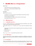
Rotary Flexible Link
Workbook
FLEXGAGE
Student Version
Quanser Inc.
2011
c 2011 Quanser Inc., All rights reserved.
⃝
Quanser Inc.
119 Spy Court
Markham, Ontario
L3R 5H6
Canada
[email protected]
Phone: 1-905-940-3575
Fax: 1-905-940-3576
Printed in Markham, Ontario.
For more information on the solutions Quanser Inc. offers, please visit the web site at:
http://www.quanser.com
This document and the software described in it are provided subject to a license agreement. Neither the software nor this document may be
used or copied except as specified under the terms of that license agreement. All rights are reserved and no part may be reproduced, stored in
a retrieval system or transmitted in any form or by any means, electronic, mechanical, photocopying, recording, or otherwise, without the prior
written permission of Quanser Inc.
ACKNOWLEDGEMENTS
Quanser, Inc. would like to thank Dr. Hakan Gurocak, Washington State University Vancouver, USA, for his help to include embedded outcomes assessment.
FLEXGAGE Workbook - Student Version
2
CONTENTS
1
Introduction
2
Modeling
2.1
Background
2.2
Pre-Lab Questions
2.3
Lab Experiments
2.4
Results
5
5
10
11
15
3
Control Design
3.1
Specifications
3.2
Background
3.3
Pre-Lab Questions
3.4
Lab Experiments
3.5
Results
16
16
16
18
19
23
4
System Requirements
4.1
Overview of Files
4.2
Setup for Finding Stiffness
4.3
Setup for Model Validation
4.4
Setup for Flexible Link Control Simulation
4.5
Setup for Flexible Link Control Implementation
24
25
25
26
26
27
5
Lab Report
5.1
Template for Content (Modeling)
5.2
Template for Content (Control)
5.3
Tips for Report Format
28
28
29
30
FLEXGAGE Workbook - Student Version
4
v 1.0
1
INTRODUCTION
The objective of this experiment is to control the position of the servo while minimizing the motions the flexible rotary
link.
Topics Covered
• Modeling the Rotary Flexible Link using Lagrange.
• Find the linear state-space model of the system.
• Do some basic model validation.
• Design an state-feedback controller using Linear-Quadratic Regulator (LQR) algorithm through simulation.
• Implement the designed LQR controller on the device.
• Compare the simulated and measured closed-loop results.
• Assess the behaviour of implementing a partial-state feedback controller.
Prerequisites
In order to successfully carry out this laboratory, the user should be familiar with the following:
• Basics of Simulinkr .
• Transfer function fundamentals.
• State-space modeling, e.g., obtaining state equations from a set of differential equations.
• SRV02 QUARC Integration Laboratory ([2]) in order to be familiar using QUARCr with the SRV02.
FLEXGAGE Workbook - Student Version
4
2
MODELING
2.1 Background
2.1.1 Model
The Rotary Flexible Link model is shown in Figure 2.1. The base of the flexible link is mounted on the load gear of
the SRV02 system. The servo angle, θ, increases positively when it rotates counter-clockwise (CCW). The servo
(and thus the link) turn in the CCW direction when the control voltage is positive, i.e., Vm > 0.
The flexible link has a total length of Ll , a mass of ml , and its moment of inertia about the center of mass is Jl . See
the Rotary Flexible Link User Manual (in [7]) for the values of these parameters. The deflection angle of the link is
denoted as α and increases positively when rotated CCW.
Figure 2.1: Rotary Flexible Link Angles
The flexible link system can be represented by the diagram shown in Figure 2.2. Our control variable is the input
servo motor voltage, Vm . This generates a torque, τ , at the load gear of the servo that rotates the base of the link.
The viscous friction coefficient of the servo is denoted by Beq . This is the friction that opposes the torque being
applied at the servo load gear. The friction acting on the link is represented by the viscous damping coefficient Bl .
Finally, the flexible link is modeled as a linear spring with the stiffness Ks .
Figure 2.2: Rotary Flexible Link Model
FLEXGAGE Workbook - Student Version
v 1.0
2.1.2 Finding the Equations of Motion
Instead of using classical mechanics, the Lagrange method is used to find the equations of motion of the system.
This systematic method is often used for more complicated systems such as robot manipulators with multiple joints.
More specifically, the equations that describe the motions of the servo and the link with respect to the servo motor
voltage, i.e. the dynamics, will be obtained using the Euler-Lagrange equation:
∂2L
∂L
−
= Qi
∂t∂ q˙i
∂qi
(2.1)
The variables qi are called generalized coordinates. For this system let
q(t)⊤ = [θ(t) α(t)]
(2.2)
where, as shown in Figure 2.2, θ(t) is the servo angle and α(t) is the flexible link angle. The corresponding velocities
are
[
]
∂θ(t) ∂α(t)
q̇(t)⊤ =
(2.3)
∂t
∂t
Note: The dot convention for the time derivative will be used throughout this document, i.e., θ̇ =
The time variable t will also be dropped from θ and α, i.e., θ := θ(t) and α := α(t).
dθ
dt
and α̇ =
dα
dt .
With the generalized coordinates defined, the Euler-Lagrange equations for the rotary flexible link system are
and
∂2L
∂L
−
= Q1
∂θ
∂t∂ θ̇
(2.4)
∂2L
∂L
−
= Q2
∂t∂ α̇ ∂α
(2.5)
L=T −V
(2.6)
The Lagrangian of a system is defined
where T is the total kinetic energy of the system and V is the total potential energy of the system. Thus the Lagrangian
is the difference between a system's kinetic and potential energies.
The generalized forces Qi are used to describe the non-conservative forces (e.g., friction) applied to a system with
respect to the generalized coordinates. In this case, the generalized force acting on the rotary arm is
Q1 = τ − Beq θ̇
(2.7)
Q2 = −Bl α̇.
(2.8)
and acting on the link is
The torque applied at the base of the rotary arm (i.e., at the load gear) is generated by the servo motor as described
by the equation
ηg Kg ηm kt (Vm − Kg km θ̇)
τ=
.
(2.9)
Rm
See [4] for a description of the corresponding SRV02 parameters (e.g. such as the back-emf constant, km ). The
servo damping (i.e. friction), Beq , opposes the applied torque. The flexible link is not actuated, the only force acting
on the link is the damping, Bl .
Again, the Euler-Lagrange equations is a systematic method of finding the equations of motion (EOMs) of a system.
Once the kinetic and potential energy are obtained and the Lagrangian is found, then the task is to compute various
derivatives to get the EOMs.
FLEXGAGE Workbook - Student Version
6
2.1.3 Potential and Kinetic Energy
Kinetic Energy
Translational kinetic equation is defined as
1
mv 2 ,
2
where m is the mass of the object and v is the linear velocity.
T =
(2.10)
Rotational kinetic energy is described as
1 2
Jω
2
where J is the moment of inertia of the object and ω is its angular rate.
T =
(2.11)
Potential Energy
Potential energy comes in different forms. Typically in mechanical system we deal with gravitational and elastic
potential energy. The relative gravitational potential energy of an object is
Vg = mg∆h,
(2.12)
where m is the object mass and ∆h is the change in altitude of the object (from a reference point). The potential
energy of an object that rises from the table surface (i.e., the reference) up to 0.25 meter is ∆h = 0.25 − 0 = 0.25
and the energy stored is Vg = 0.25mg.
The equation for elastic potential energy, i.e., the energy stored in a spring, is
Ve =
1
K∆x2
2
(2.13)
where K is the spring stiffness and ∆x is the linear or angular change in position. If an object that is connected to
a spring moves from in its initial reference position to 0.1 m, then the change in displacement is ∆x = 0.1 − 0 = 0.1
and the energy stored equals Ve = 0.005K.
2.1.4 Linear State-Space Model
The linear state-space equations are
ẋ = Ax + Bu
(2.14)
y = Cx + Du
(2.15)
and
where x is the state, u is the control input, A, B, C, and D are state-space matrices. For the Rotary Flexible Link
system, the state and output are defined
x⊤ = [θ α θ̇ α̇]
(2.16)
and
y ⊤ = [x1 x2 ].
(2.17)
In the output equation, only the position of the servo and link angles are being measured. Based on this, the C and
D matrices in the output equation are
[
]
1 0 0 0
C=
(2.18)
0 1 0 0
and
D=
[ ]
0
.
0
(2.19)
The velocities of the servo and link angles can be computed in the digital controller, e.g., by taking the derivative
and filtering the result though a high-pass filter.
FLEXGAGE Workbook - Student Version
v 1.0
2.1.5 Free-Oscillation of a Second Order System
The free-oscillatory equation of motion of a second-order system described by
(2.20)
J ẍ + B ẋ + Kx = 0
is shown in Figure 2.3. Assuming the initial conditions x(0− ) = x0 and ẋ(0− ) = 0, the Laplace transform of Equation
2.20 is
x
0
X(s) =
s2 +
J
B
Js
+
(2.21)
K
J
Figure 2.3: Free Oscillation Response
The prototype second-order equation is defined
s2 + 2ζωn s + ωn2 ,
(2.22)
where ζ is the damping ratio and ωn is the natural frequency. Equating the characteristic equation in 2.21 to this
gives
K
ωn2 =
(2.23)
J
and
B
2ζωn =
(2.24)
J
Based on the measured damping ratio and natural frequency, the friction (or stiffness) of the system is
K = Jωn2
(2.25)
B = 2ζωn J.
(2.26)
and the viscous damping is
Finding the Natural Frequency
The period of the oscillations in a system response can be found using the equation
Tosc =
tn+1 − t1
n
FLEXGAGE Workbook - Student Version
(2.27)
8
where tn is the time of the nth oscillation, t1 is the time of the first peak, and n is the number of oscillations considered.
From this, the damped natural frequency (in radians per second) is
ωd =
and the undamped natural frequency is
2π
Tosc
ωd
ωn = √
.
1 − ζ2
(2.28)
(2.29)
Finding the Damping Ratio
The damping ratio of a second-order system can be found from its response. For a typical second-order underdamped system, the subsidence ratio (i.e., decrement ratio) is defined as
δ=
1 O1
ln
n On
(2.30)
where O1 is the peak of the first oscillation and On is the peak of the nth oscillation. Note that O1 > On , as this is a
decaying response.
The damping ratio is defined
1
ζ=√
1+
FLEXGAGE Workbook - Student Version
2π 2
δ
(2.31)
v 1.0
2.2 Pre-Lab Questions
1. Energy is stored in the flexible link, i.e., the "spring", as it flexes by an angle of α (see Figure 2.1). Find the
potential energy of the flexible link. Use the parameters shown in Figure 2.2.
2. Find the total kinetic energy of the system contributed by the rotary servo, θ, and the deflection in the link, α.
Use the parameters shown in Figure 2.2.
3. Compute the Lagrangian of the system.
4. Find the first Euler-Lagrange equation given in 2.4. Keep the equations in terms of applied torque, τ (i.e., not
in terms of DC motor voltage). Also make sure your equations follow the general form: J ẍ + B ẋ + Kx = u.
5. Find the second Euler-Lagrange Equation 2.5.
6. Find the equations of motion: θ̈ = f1 (θ, θ̇, α, α̇, τ ) and α̈ = f2 (θ, θ̇, α, α̇, τ ). Assume the viscous damping of the
link is negligible, i.e., Bl = 0.
7. Given state x defined in Equation 2.16, find the linear state-space matrices A and B.
8. Find the the natural frequency of the response shown in Figure 2.3 if the peak values for the first and fifth
oscillation are: t1 = 1.12 and t5 = 1.71 seconds. Because the damping is low, assume the damped and
undamped natural frequency are equivalent.
FLEXGAGE Workbook - Student Version
10
2.3 Lab Experiments
In the first part of this laboratory, the stiffness of the flexible link is determined by measuring its natural frequency. In
the second part, the state-space model is finalized and validated against actual measurements.
2.3.1 Finding Stiffness
In Section 2.1.5 we found an equation describing the free-oscillation response of a second-order system. This can
also be used to describe the response of the flexible link when initially perturbed and left to decay.
Physical Parameters for the Lab
In order to do some of the laboratory exercises, you will need these values:
Beq
Jeq
ml
Ll
= 0.004 N · m / (rad/s)
= 2.08 × 10−3 kg · m2
= 0.065 kg
= 0.419 m
Note: The equivalent viscous damping, Beq , and moment of inertia, Jeq , parameters are for the SRV02 when there
is no load (i.e., the parameter found in the SRV02 Modeling Laboratory was for servo with the disc load).
Experimental Setup
The q flexgage id Simulink diagram shown in Figure 2.4 is used to find the natural frequency of the flexible link. The
QUARC blocks are used to interface with strain gage sensor of the system. For more information about QUARC,
see Reference [2]. This model outputs the deflection angle of the link.
Figure 2.4: q flexage id Simulink diagram used to find link stiffness
IMPORTANT: Before you can conduct this experiment, you need to make sure that the lab files are configured
according to your system setup. If they have not been configured already, then you need to go to Section 4.2 to
configure the lab files first.
1. In the q flexgage id Simulink diagram, go to QUARC | Build to build the QUARC controller.
2. Hold on the SRV02 load gear, go to QUARC | Start to run the controller, and then immediately perturb the
flexible link. Keep holding the SRV02 base until the controller is done collecting the data. The alpha (deg)
Scope should be reading a response similarly as shown in Figure 2.5. Note that the controller is set to run for
5 seconds.
FLEXGAGE Workbook - Student Version
v 1.0
Figure 2.5: Typical Flexible Link Free-Oscillation Response
3. After the controller stops (i.e., after 5 sec), the data is automatically saved in the Matlab workspace to the
variable data alpha. The time is stored in data alpha(:,1) vector and the flexible link angle is stored the
data alpha(:,2) vector. Plot the response in a Matlab figure.
4. Find the natural frequency of the link. As in Pre-Lab Question 8, the damping in low. Therefore assume the
damped natural frequency (which is being measured) is equivalent to the undamped natural frequency.
5. Calculate the stiffness of the flexible link, Ks .
Hint: Assume the link is a rod when finding the moment of inertia of the link, Jl .
2.3.2 Model Validation
By running a simulation and the actual device in parallel, we can verify whether the dynamic model (which drives
the simulation) accurately represents our system.
Experimental Setup
The q flexgage val Simulink diagram shown in Figure 2.6 applies either a step or pulse input to both the Quanser
Flexible Link hardware and to the Flexible Link model and reads the servo and link angles. The SRV02 Flexible
Link subsystem contains the QUARC blocks that interface to the actual hardware. The Simulink State-Space block
reads the A, B, C, and D state-space matrices that are loaded in the Matlab workspace. This model outputs the
deflection angle of the link.
IMPORTANT: Before you can conduct this experiment, you need to make sure that the lab files are configured
according to your system setup. If they have not been configured already, then go to Section 4.3 to configure the
lab files first.
1. Run the setup flexgage.m.
2. When prompted, enter the stiffness you found in Section 2.3.1. This is saved to the Matlab variable Ks.
Enter link stiffness (Ks):
3. Depending on your stiffness, the Matlab prompt should generate a gain similarly as shown below (this gain is
generated for a Ks of 1):
FLEXGAGE Workbook - Student Version
12
Figure 2.6: q flexage val Simulink diagram used validate the model
K =
1.0000
-8.7209
0.6264
-0.3958
This means the script ran correctly.
4. In Matlab, open the M-File called FLEXGAGE ABCD eqns student.m. The script has the following state-space
matrices entered:
A = [0 0 1 0;
0 0 0 1;
0 500 -5 0;
0 -750 5 0];
B = [0 0 500 -500]';
C = zeros(2,4);
D = zeros(2,1);
5. Enter the state-space matrices you found in Section 2.2 for A, B, C, and D. In Matlab, the stiffness and link
moment of inertia are defined as Ks and Jl and the SRV02 inertia and damping are denoted Jeq and Beq.
6. Run the FLEXGAGE ABCD eqns student.m script to load the state-space matrices in the Matlab workspace.
Show the numerical matrices that are displayed in the Matlab prompt.
7. The input of the state-space model you found in Section 2.2 is the torque acting at the servo load gear (or
the pivot of the flexible link). However, we do not control torque directly - we control the servo input voltage.
Recall the voltage-torque relationship given in Equation 2.9 in Section 2.1.2. In the System Model section of
the setup flexgage.m script, the actuator dynamics are added to your state-space matrices with the code:
Ao = A;
Bo = B;
B = eta_g*Kg*eta_m*kt/Rm*Bo;
A(3,3) = Ao(3,3) - Bo(3)*eta_g*Kg^2*eta_m*kt*km/Rm;
A(4,3) = Ao(4,3) - Bo(4)*eta_g*Kg^2*eta_m*kt*km/Rm;
8. Run the setup flexgage.m script again so your Flexible Link model is based on dc motor voltage.
FLEXGAGE Workbook - Student Version
v 1.0
9. In the q flexgage val Simulink diagram, go to QUARC | Build to build the QUARC controller.
10. Make sure the area around the Flexible Link experiment is clear. Set the Manual Switch to the downward
position to feed a Step input.
11. Go to QUARC | Start to run the q flexgage val controller. Typical scope responses are shown in Figure 2.7a
and Figure 2.7b. The theta (deg) scope displays the simulated servo angle in yellow and the measured angle
in purple. Similarly, the alpha (deg) scope shows the simulated link angle in yellow and the measured angle
in purple.
(a) Servo Angle
(b) Flexible Link Angle
Figure 2.7: Typical Flexible Link Model Validation Response
12. If your simulation and measured response match, go to the next step. If they do not, then there is an issue
with your model. Here are some issues to investigate:
• Ensure the state-space model was enterred properly in the script.
• The stiffness, Ks , found in Section 2.3.1 is not correct. Review your calculations or redo the experiment.
• Review your model derivation in Section 2.2, e.g., might be a mistake in solving the EOMs.
13. The theta (deg) and alpha (deg) scopes save their data to the variables data theta and data alpha. For
data theta, the time is in data theta(:,1), the simulated servo angle is in data theta(:,2), and the measured
SRV02 angle is in data theta(:,3). Similarly for the flexible link response saved in data alpha. Plot the response in a Matlab figure.
14. How well does your model represent the actual system? We want a model that is fairly representative but,
having said that, keep in mind that no model is perfect. This is just a quick test to see how well your model
represents the actual device. As shown in figures 2.7a and 2.7b, the simulation does not match the measured
response perfectly.
15. Give at least one reason why the model does not represent the system accurately.
16. In Matlab, find the open-loop poles (i.e., eigenvalues) of the system using the state-space matrix A that is
loaded.
Note: These will be required for a pre-lab question in Section 3.3.
FLEXGAGE Workbook - Student Version
14
2.4 Results
Fill out Table 1 with your answers from your modeling lab results - both simulation and implementation.
Description
Finding Stiffness
Natural frequency
Stiffness
Model Validation
Symbol
State-Space Matrix
A
State-Space Matrix
B
State-Space Matrix
C
State-Space Matrix
D
Open-loop poles
OL
Value
Unit
rad/s
N m/rad
ωn
Ks
Table 1: Results
FLEXGAGE Workbook - Student Version
v 1.0
3
CONTROL DESIGN
3.1 Specifications
The time-domain requirements are:
Specification 1: Servo angle settling time: ts <= 0.5 s.
Specification 2: Servo angle percentage overshoot: P O <= 7.5 %.
Specification 3: Maximum link angle deflection: |α| <= 10 deg.
Specification 4: Maximum control effort / voltage: |Vm | <= 10 V.
These specifications are to be satisfied when the rotary arm is tracking a ±30 degree angle square wave.
3.2 Background
In Section 2.2, we found a linear state-state space model that represents the Rotary Flexible Link system. This
model is used to investigate the stability properties of the Flexible Link system in Section 3.2.1. In Section 3.2.2,
the notion of controllability is introduced. Using the Linear Quadratic Regular algorithm, or LQR, is a common way
to find the control gain and is discussed in Section 3.2.3. Lastly, Section 3.2.4 describes the state-feedback control
used to control the servo position while minimizing link deflection.
3.2.1 Stability
The stability of a system can be determined from its poles ([8]):
• Stable systems have poles only in the left-hand plane.
• Unstable systems have at least one pole in the right-hand plane and/or poles of multiplicity greater than 1 on
the imaginary axis.
• Marginally stable systems have one pole on the imaginary axis and the other poles in the left-hand plane.
The poles are the roots of the system's characteristic equation. From the state-space, the characteristic equation of
the system can be found using
det (sI − A) = 0
(3.1)
where det() is the determinant function, s is the Laplace operator, and I the identity matrix. These are the eigenvalues
of the state-space matrix A.
3.2.2 Controllability
If the control input, u, of a system can take each state variable, xi where i = 1 . . . n, from an initial state to a final
state then the system is controllable, otherwise it is uncontrollable ([8]).
Rank Test The system is controllable if the rank of its controllability matrix
[
]
T = B AB A2 B . . . An B
(3.2)
equals the number of states in the system,
rank(T ) = n.
FLEXGAGE Workbook - Student Version
(3.3)
16
3.2.3 Linear Quadratic Regular (LQR)
If (A,B) are controllable, then the Linear Quadratic Regular optimization method can be used to find a feedback
control gain. Given the plant model in Equation 2.14, find a control input u that minimizes the cost function
∫ ∞
J=
x(t)′ Qx(t) + u(t)′ Ru(t) dt,
(3.4)
0
where Q and R are the weighting matrices. The weighting matrices affect how LQR minimizes the function and are,
essentially, tuning variables.
Given the control law u = −Kx, the state-space in Equation 2.14 becomes
ẋ
= Ax + B(−Kx)
= (A − BK)x
3.2.4 Feedback Control
The feedback control loop that in Figure 3.1 is designed to stabilize the servo to a desired position, θd , while minimizing the deflection of the flexible link.
The reference state is defined
xd = [θd 0 0 0]
(3.5)
u = K(xd − x).
(3.6)
and the controller is
Note that if xd = 0 then u = −Kx, which is the control used in the LQR algorithm.
Figure 3.1: State-feedback control loop
FLEXGAGE Workbook - Student Version
v 1.0
3.3 Pre-Lab Questions
1. Based on your analysis of the system in the Modeling Laboratory (Section 2.3), is the system stable, marginally
stable, or unstable? From your experience in Section 2.3, does the stability you determined analyically match
how the actual system behaves?
2. Designing a controller with the Linear Quadratic Regular (LQR) technique is an iterative process. In software,
you have to tune the Q and R matrices, generate the gain K using LQR, and either simulate the system or
implement the control to see if you have the desired response. The relationship between changing Q and R
and the closed-loop response is not evident. However, we can have a better idea on how changing the different
elements in Q and R will effect the response. We will only be changing the diagonal elements in Q, thus let


q1 0 0 0
 0 q2 0 0 

(3.7)
Q=
 0 0 q3 0  .
0 0 0 q4
Since we are dealing with a single-input system, R is a scalar value. Using the Q and R defined, expand the
cost function given in Equation 3.4.
3. For the feedback control u = −Kx, the Linear-Quadratic Regular algorithm finds a gain K that minimizes the
cost function J. Matrix Q sets the weight on the states and determines how u will minimize J (and hence how it
generates gain K). From your solution in Question 2, explain how increasing the diagonal elements, qi , effects
the generated gain K = [k1 k2 k3 k4 ].
4. Explain the effect of increasing R has on the generated gain, K.
FLEXGAGE Workbook - Student Version
18
3.4 Lab Experiments
The control gain is designed using LQR through simulation first. Once a gain that satisfies the requirements is found,
it is implemented on the actual Quanser Flexible Link system.
3.4.1 Control Simulation
Using the linear state-space model of the system and the designed control gain, the closed-loop response can be
simulated. This way, we can test the controller and see if it satisfies the given specifications before running it on the
hardware platform.
Experiment Setup
The s flexgage Simulink diagram shown in Figure 3.2 is used to simulate the closed-loop response of the Flexible
Link using the LQR control developed in Section 3.3.
The Smooth Signal Generator block generates a 0.33 Hz square wave (with amplitude of 1) that is passed through
a Rate Limiter block to smooth the signal. The Amplitude (deg) gain block is used to change the desired servo
position command. The state-feedback gain K is set in the LQR Control gain block and is read from the Matlab
workspace. The Simulink State-Space block reads the A, B, C, and D state-space matrices that are loaded in the
Matlab workspace.
Figure 3.2: s flexgage Simulink diagram used to simulate the state-feedback control
IMPORTANT: Before you can conduct this experiment, you need to make sure that the lab files are configured according to your system setup. If they have not been configured already, go to Section Section 4.4 to configure the lab
files first. Make sure the model you found in Section 2.3.2 is enterred in FLEXGAGE ABCD eqns student.m.
1. Open setup flexgage.m and go down to the LQR Control section shown here:
%% LQR Control
if strcmp ( CONTROL_TYPE , 'MANUAL' )
% Set Q and R matrices to get desired response.
Q = diag([1 1 1 1]);
R = 1;
[K,S,E] = lqr(A,B,Q,R);
FLEXGAGE Workbook - Student Version
v 1.0
The Q and R are initially set to the default values of:

1
 0
Q = 
 0
0
R = 1.
0
1
0
0
0
0
1
0

0
0 
 and
0 
1
2. These will not give you the desired response, but run the script to generate the default gain K. Enter the
stiffness you found in Section 2.3.1 when prompted.
3. Run s flexgage to simulated the closed-loop response with this gain. See figures 3.3a, 3.3b, and 3.3c for the
typical response.
(a) Servo Angle
(b) Flexible Link Angle
(c) Voltage
Figure 3.3: Default Simulated Closed-Loop Response
4. If Q = diag[q1 , q2 , q3 , q4 ], vary each qi independently and examine its effect on the gain and the closed-loop
response. For example, when increasing q3 , what happens to θ and α? Vary each qi by the same order of
magnitude and compare how the new gain K changes compared to the original gain. Keep R = 1 throughout
your testing. Summarize your results.
Note: Recall your analysis in pre-lab Question 3 where the effect of adjusting Q on the generated K was
assessed generally by inspecting the cost function equation. You may find some discrepancies in this exercise
and the pre-lab questions.
5. Find a Q and R that will satisfy the specifications given in Section 3.1. When doing this, don't forget to keep
the dc motor voltage within ±10 V. This control will later be implemented on actual hardware. Therefore, make
sure the actuator is not being saturated. Enter the weighting matrices, Q and R, used and the resulting gain,
K.
6. Plot the responses from the theta (deg), alpha (deg), and Vm (V) scopes in a Matlab figure. When the QUARC
controller is stopped, these scopes automatically save the last 5 seconds of their response data to the variables
data theta, data alpha, and data vm. For data theta, the time is in data theta(:,1), the setpoint (i.e., desired
SRV02 angle) is in data theta(:,2), and the simulated SRV02 angle is in data theta(:,3). In the data alpha and
data vm variables, the (:,1) holds the time vector and the (:,2) holds the actual measured data.
7. Measure the settling time and percent overshoot of the simulated servo response and the maximum link deflection. Does the response satisfy the specifications given in Section 3.1?
8. Briefly explain the procedure you used to find Q and R.
3.4.2 Control Implementation
In this experiment, the servo position is controlled while minimizing the link deflection using the LQR-based control
found in Section 3.4.1. Measurements will then be taken to ensure that the specifications are satisfied.
FLEXGAGE Workbook - Student Version
20
Experiment Setup
The q flexgage Simulink diagram shown in Figure 3.4 is used to run the state-feedback control on the Quanser
Flexible Link system. The SRV02 Flexible Link subsystem contains QUARC blocks that interface with the DC motor
and sensors of the system. The feedback developed in Section 3.4.1 is implemented using a Simulink Gain block.
Figure 3.4: q flexgage Simulink diagram used the model
IMPORTANT: Before you can conduct this experiment, you need to make sure that the lab files are configured
according to your system setup. If they have not been configured already, then go to Section 4.5 to configure the
lab files first.
1. Run the setup flexgage.m.
2. Ensure the LQR controller you found in Section 3.4.1 is loaded, i.e., gain K.
3. Open the q flexgage Simulink diagram. Make sure the Manual Switch is set to the Full-State Feedback (upward) position.
4. Go to QUARC | Build to build the controller.
5. Go to QUARC | Start to run the controller. The flexible link should be tracking the default ± 30 degree signal.
6. Stop the controller once you have obtained a representative response.
7. Plot the responses from the theta (deg), alpha (deg), and Vm (V) scopes in a Matlab figure. Similarly as
described in Section 3.4.1, the response data is saved in variables data theta, data alpha, and data vm.
8. Measure the settling time and percent overshoot of the measured servo response and the maximum link
deflection. Does the response satisfy the specifications given in Section 3.1?
9. If the specifications have been met, then you can proceed to Section 3.4.3 or your report (ask your instructor).
If they have not been met, then you need to tweak your controller. Using the principles you learnt in Section
3.4.1, tune the current Q and R matrices to satisfy the specifications. Enter the weighting matrices, Q and R,
used and the resulting gain, K.
10. Plot the responses from the theta (deg), alpha (deg), and Vm (V) scopes in a Matlab figure of your newly
tuned controller. Similarly as described in Section 3.4.1, the response data is saved in variables data theta,
data alpha, and data vm.
11. Measure the settling time and percent overshoot of the simulated servo response and the maximum link deflection. Does the response satisfy the specifications given in Section 3.1?
12. Explain the procedure you used to tune your controller.
FLEXGAGE Workbook - Student Version
v 1.0
3.4.3 Implementing Partial-State Feedback Control
In this section, the partial-state feedback response of the system is assessed and compared with the full-state
feedback control in Section 3.4.2.
1. Run the setup flexgage.m.
2. Ensure the LQR control gain you settled on in Section 3.4.2 is loaded, i.e., gain K.
3. Open the q flexgage Simulink diagram. Make sure the Manual Switch is set to the Partial-State Feedback
(downward) position.
4. Go to QUARC | Start to run the controller. The flexible link should be tracking the default ±30 degree signal.
5. Stop the controller once you have obtained a representative response.
6. As in Section 3.4.2, attach a Matlab figure representing the SRV02 angle and flexible link angle response, as
well as the input voltage.
7. Examine the difference between the partial-state feedback (PSF) response and the full-state feedback (FSF)
response. Explain why PSF control behaves this way by looking at the q flexgage Simulink diagram.
FLEXGAGE Workbook - Student Version
22
3.5 Results
Fill out Table 2 with your answers from your control lab results - both simulation and implementation.
Description
LQR Simulation
Symbol
LQR Weighting Matrices
Q
LQR Gain
Settling time
Percentage overshoot
Maximum deflection
LQR Implementation
Value
R
K
ts
PO
|α|max
LQR Weighting Matrices
Q
LQR Gain
Settling time
Percentage overshoot
Maximum deflection
R
K
ts
PO
|α|max
Unit
s
%
deg
s
%
deg
Table 2: Results
FLEXGAGE Workbook - Student Version
v 1.0
4
SYSTEM REQUIREMENTS
Required Software
• Microsoft Visual Studio
• Matlabr with Simulinkr , Real-Time Workshop, and the Control System Toolbox.
• QUARCr 2.1, or later.
See the QUARCr software compatibility chart at [5] to see what versions of MS VS and Matlab are compatible with
your version of QUARC and for what OS.
Required Hardware
• Data-acquisition (DAQ) card that is compatible with QUARC. This includes Quanser Hardware-in-the-loop
(HIL) boards such as:
– Q2-USB
– Q8-USB
– QPID
– QPIDe
and some National Instruments DAQ devices (e.g., NI USB-6251, NI PCIe-6259). For a full listing of compliant
DAQ cards, see Reference [1].
• Quanser SRV02-ET rotary servo.
• Quanser Rotary Flexible Joint (attached to SRV02).
• Quanser VoltPAQ-X1 power amplifier, or equivalent.
Before Starting Lab
Before you begin this laboratory make sure:
• QUARCr is installed on your PC, as described in [3].
• The QUARC Analog Loopback Demo has been ran successfully.
• SRV02 Rotary Flexible Joint and amplifier are connected to your DAQ board as described Reference [7].
FLEXGAGE Workbook - Student Version
24
4.1 Overview of Files
File Name
Flexible Link User Manual.pdf
Flexible Link Workbook (Student).pdf
setup flexgage.m
config srv02.m
config flexgage.m
d model param.m
FLEXGAGE ABCD eqns student.m
calc conversion constants.m
s flexgage.mdl
q flexgage id.mdl
q flexgage val.mdl
q flexgage.mdl
Description
This manual describes the hardware of the Rotary Flexible Link system and explains how to setup and wire the
system for the experiments.
This laboratory guide contains pre-lab questions and lab
experiments demonstrating how to design and implement
a position controller on the Quanser SRV02 Flexible Link
plant using QUARCr .
The main Matlab script that sets the SRV02 motor and
sensor parameters, the SRV02 configuration-dependent
model parameters, and the Flexible Link (i.e., flexgage)
sensor parameters. Run this file only to setup the laboratory.
Returns the configuration-based SRV02 model specifications Rm, kt, km, Kg, eta g, Beq, Jeq, and eta m, the
sensor calibration constants K POT, K ENC, and K TACH,
and the amplifier limits VMAX AMP and IMAX AMP.
Returns the Flexible Link model inertial, Jl , viscous damping, Bl , and sensor calibration constant K GAGE.
Calculates the SRV02 model parameters K and tau based
on the device specifications Rm, kt, km, Kg, eta g, Beq,
Jeq, and eta m.
Contains the incomplete state-space A, B, C, and D matrices. These are used to represent the Flexible Link system.
Returns various conversions factors.
Simulink file that simulates the Flexible Link system when
using a full or partial state-feedback control.
When ran with QUARCr , this Simulink model measures
the Flexible Link angle. The measured response can then
be used to find the stiffness of the link.
This Simulink model is used with QUARCr to compare
the Flexible Link state-space model with the measured response from the actual system.
Simulink file that implements a closed-loop state-feedback
controller on the actual FLEXGAGE system using
QUARCr .
Table 3: Files supplied with the SRV02 Flexible Link Control Laboratory.
4.2 Setup for Finding Stiffness
Before beginning in-lab procedure outlined in Section 2.3.1, the q flexgage id Simulink diagram must be properly
configured.
Follow these steps:
1. Setup the SRV02 with the Flexible Link module as detailed in the Flexible Link User Manual ([7]).
2. Load the Matlab software.
3. Browse through the Current Directory window in Matlab and find the folder that contains the file q flexgage id.mdl.
4. Open the q flexgage id.mdl Simulink diagram, shown in Figure 2.4.
FLEXGAGE Workbook - Student Version
v 1.0
5. Configure DAQ: Ensure the HIL Initialize block subsystem is configured for the DAQ device that is installed
in your system. By default, the block is setup for the Quanser Q8 hardware-in-the-loop board. See Reference
[1] for more information on configuring the HIL Initialize block.
4.3 Setup for Model Validation
Before performing the in-lab exercises in Section 2.3.2, the q flexgage val Simulink diagram and the setup flexgage.m
script must be configured.
Follow these steps to get the system ready for this lab:
1. Setup the SRV02 with the Flexible Link module as detailed in [7].
2. Load the Matlab software.
3. Browse through the Current Directory window in Matlab and find the folder that contains the QUARC FLEXGAGE file q flexgage val.mdl.
4. Open the q flexgage val.mdl Simulink diagram, shown in Figure 2.6.
5. Configure DAQ: Ensure the HIL Initialize block in the SRV02 Flexible Link subsystem is configured for the
DAQ device that is installed in your system. By default, the block is setup for the Quanser Q8 hardware-inthe-loop board. See Reference [1] for more information on configuring the HIL Initialize block.
6. Configure Sensor: The position of the SRV02 load shaft can be measured using either the potentiometer or
the encoder. Set the Pos Src Source block in q flexgage val, as shown in Figure 2.6, as follows:
• 1 to use the potentiometer
• 2 to use to the encoder
Note that when using the potentiometer, there will be a discontinuity.
7. Configure Input: Set the Manual Switch to the DOWN position for a step input or the UP position for a square
signal.
8. Open the setup flexgage.m file. This is the setup script used for the FLEXGAGE Simulink models.
9. Configure setup script: When used with the Flexible Link, the SRV02 has no load (i.e., no disc or bar) and
has to be in the high-gear configuration. Make sure the script is setup to match this setup:
• EXT GEAR CONFIG to 'HIGH'
• LOAD TYPE to 'NONE'
• Ensure ENCODER TYPE, TACH OPTION, K CABLE, AMP TYPE, and VMAX DAC parameters are set
according to the SRV02 system that is to be used in the laboratory.
• CONTROL TYPE to 'MANUAL'.
4.4 Setup for Flexible Link Control Simulation
Before going through the control simulation in Section 3.4.1, the s flexgage Simulink diagram and the setup flexgage.m
script must be configured.
Follow these steps to configure the lab properly:
1. Load the Matlab software.
FLEXGAGE Workbook - Student Version
26
2. IMPORTANT: Make sure the model you found in Section 2.3.2 is enterred in FLEXGAGE ABCD eqns
student.m.
3. Browse through the Current Directory window in Matlab and find the folder that contains the s flexgage.mdl
file.
4. Open s flexgage.mdl Simulink diagram shown in Figure 3.2.
5. Configure the setup flexgage.m script according to your hardware. See Section 4.3 for more information.
6. Run the setup flexgage.m script.
7. Enter the stiffness (Ks) you found in Section 2.3.1.
4.5 Setup for Flexible Link Control Implementation
Before beginning the in-lab exercises given in Section 3.4.2 (or Section 3.4.3), the q flexgage Simulink diagram and
the setup flexgage.m script must be setup.
Follow these steps to get the system ready for this lab:
1. Setup the SRV02 with the Flexible Link module as detailed in [7] .
2. Load the Matlab software.
3. Browse through the Current Directory window in Matlab and find the folder that contains the q flexgage.mdl
file.
4. Open the q flexgage.mdl Simulink diagram shown in Figure 3.4.
5. Configure DAQ: Ensure the HIL Initialize block in the SRV02 Flexible Link subsystem is configured for the
DAQ device that is installed in your system. By default, the block is setup for the Quanser Q8 hardware-inthe-loop board. See Reference [1] for more information on configuring the HIL Initialize block.
6. Configure Sensor: The position of the SRV02 load shaft can be measured using the potentiometer or the
encoder. Set the Pos Src Source block in q flexgage, as shown in Figure 3.4, as follows:
• 1 to use the potentiometer
• 2 to use to the encoder
Note that when using the potentiometer, there will be a discontinuity.
7. Configure setup script: Set the parameters in the setup flexgage.m script according to your system setup.
See Section 4.3 for more details.
8. Run the setup flexgage.m script.
FLEXGAGE Workbook - Student Version
v 1.0
5
LAB REPORT
This laboratory contains two groups of experiments, namely,
1. Modeling the Quanser Rotary Flexible Link system, and
2. State-feedback control using LQR.
For each experiment, follow the outline corresponding to that experiment to build the content of your report. Also,
in Section 5.3 you can find some basic tips for the format of your report.
5.1 Template for Content (Modeling)
I. PROCEDURE
1. Finding Stiffness
• Briefly describe the main goal of the experiment.
• Briefly describe the experiment procedure (Section 2.3.1)
2. Model Validation
• Briefly describe the main goal of the experiment.
• Briefly describe the experiment procedure (Section 2.3.2)
II. RESULTS
Do not interpret or analyze the data in this section. Just provide the results.
1. Free-oscillation plot from step 3 in Section 2.3.1.
2. Model validation plot from step 13 in Section 2.3.2.
3. Provide applicable data collected in this laboratory (from Table 1).
III. ANALYSIS
Provide details of your calculations (methods used) for analysis for each of the following:
1. Measured link stiffness in step 5 in Section 2.3.1.
2. Model discrepancies given in step 15 in Section 2.3.2.
IV. CONCLUSIONS
Interpret your results to arrive at logical conclusions for the following:
1. How does the model compare with the actual system in step 14 of Section 2.3.2, State-space model validation.
FLEXGAGE Workbook - Student Version
28
5.2 Template for Content (Control)
I. PROCEDURE
1. Simulation
• Briefly describe the main goal of the simulation.
• Briefly describe the simulation procedure (Section 3.4.1).
• Briefly describe the procedure in step 4 of Section 3.4.1 to examine the effect of variables on the gain and
closed-loop response.
• Briefly explain the procedure used to find Q and R in step 8 of Section 3.4.1).
2. Full-State Feedback Implementation
• Briefly describe the main goal of this experiment.
• Briefly describe the experimental procedure (Section 3.4.2).
• Briefly explain the procedure used to tune the controller in step 12 of Section 3.4.3.
3. Partial-State Feedback Implementation
• Briefly describe the main goal of this experiment.
• Briefly describe the experimental procedure (Section 3.4.3).
II. RESULTS
Do not interpret or analyze the data in this section. Just provide the results.
1. Response plot from step 6 in Section 3.4.1, Full-state feedback LQR controller simulation.
2. Response plot from step 7 in Section 3.4.2, for Full-state feedback LQR controller implementation.
3. Response plot from step 10 in Section 3.4.2, for Tuned LQR full-state feedback controller implementation.
4. Response plot from step 6 in Section 3.4.3, for Partial-state feedback LQR controller implementation.
5. Provide applicable data collected in this laboratory (from Table 2).
III. ANALYSIS
Provide details of your calculations (methods used) for analysis for each of the following:
1. Settling time and percent overshoot in step 7 in Section 3.4.1, Full-state feedback LQR controller simulation.
2. Settling time and percent overshoot in step 8 in Section 3.4.2, for Full-state feedback LQR controller implementation.
3. Settling time and percent overshoot in step 11 in Section 3.4.2, for Tuned LQR full-state feedback controller
implementation.
4. Comparison between partial-state and full-state feedback in step 7 in Section 3.4.3.
IV. CONCLUSIONS
Interpret your results to arrive at logical conclusions for the following:
1. Whether the controller meets the specifications in step 7 in Section 3.4.1, Full-state feedback LQR controller
simulation.
2. Whether the controller meets the specifications in step 8 in Section 3.4.2, for Full-state feedback LQR controller
implementation.
3. Whether the controller meets the specifications in step 11 in Section 3.4.2, for Tuned LQR full-state feedback
controller implementation.
FLEXGAGE Workbook - Student Version
v 1.0
5.3 Tips for Report Format
PROFESSIONAL APPEARANCE
• Has cover page with all necessary details (title, course, student name(s), etc.)
• Each of the required sections is completed (Procedure, Results, Analysis and Conclusions).
• Typed.
• All grammar/spelling correct.
• Report layout is neat.
• Does not exceed specified maximum page limit, if any.
• Pages are numbered.
• Equations are consecutively numbered.
• Figures are numbered, axes have labels, each figure has a descriptive caption.
• Tables are numbered, they include labels, each table has a descriptive caption.
• Data are presented in a useful format (graphs, numerical, table, charts, diagrams).
• No hand drawn sketches/diagrams.
• References are cited using correct format.
FLEXGAGE Workbook - Student Version
30
REFERENCES
[1] Quanser Inc. QUARC User Manual.
[2] Quanser Inc. SRV02 QUARC Integration, 2008.
[3] Quanser Inc. QUARC Installation Guide, 2009.
[4] Quanser Inc. SRV02 User Manual, 2009.
[5] Quanser Inc. QUARC Compatibility Table, 2010.
[6] Quanser Inc. SRV02 Rotary Flexible Link User Manual, 2011.
[7] Norman S. Nise. Control Systems Engineering. John Wiley & Sons, Inc., 2008.
FLEXGAGE Workbook - Student Version
v 1.0