Download QNET DC Motor Position Control

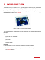
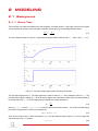
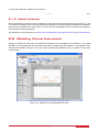
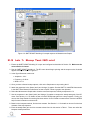
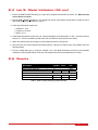
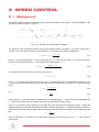
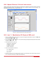
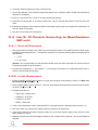
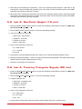
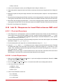
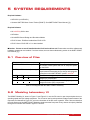
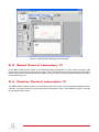
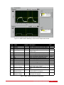
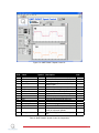
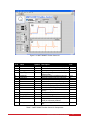
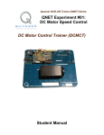
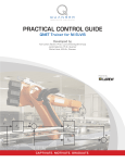
QNET DC Motor Control
Workbook
QNET DCMCT
Student Version
Quanser Inc.
2011
c 2011 Quanser Inc., All rights reserved.
⃝
Quanser Inc.
119 Spy Court
Markham, Ontario
L3R 5H6
Canada
[email protected]
Phone: 1-905-940-3575
Fax: 1-905-940-3576
Printed in Markham, Ontario.
For more information on the solutions Quanser Inc. offers, please visit the web site at:
http://www.quanser.com
This document and the software described in it are provided subject to a license agreement. Neither the software nor this document may be
used or copied except as specified under the terms of that license agreement. All rights are reserved and no part may be reproduced, stored in
a retrieval system or transmitted in any form or by any means, electronic, mechanical, photocopying, recording, or otherwise, without the prior
written permission of Quanser Inc.
Acknowledgements
Quanser, Inc. would like to thank the following contributors:
Dr. Hakan Gurocak, Washington State University Vancouver, USA, for his help to include embedded outcomes assessment, and
Dr. K. J. Åström, Lund University, Lund, Sweden for his immense contributions to the curriculum content.
QNET DCMCT Workbook - Student Version
2
Contents
1
Introduction
4
2
Modeling
2.1
Background
2.2
Modeling Virtual Instrument
2.3
Lab 1: Bump Test [60 min]
2.4
Lab 2: Model Validation [45 min]
2.5
Results
5
5
6
7
8
8
3
Speed Control
3.1
Background
3.2
Speed Control Virtual Instrument
3.3
Lab 1: Qualitative PI Control [30 min]
3.4
Lab 2: PI Control According to Specifications [60 min]
3.5
Lab 3: Set-Point Weight [15 min]
3.6
Lab 4: Tracking Triangular Signals [20 min]
3.7
Results
9
9
10
10
11
12
12
13
4
Position Control
4.1
Background
4.2
Position Control Virtual Instrument
4.3
Lab 1: Qualitative PD Control [30 min]
4.4
Lab 2: PD Control according to Specifications [60 min]
4.5
Lab 3: Response to Load Disturbance [60 min]
4.6
Results
14
14
16
16
17
18
19
5
System Requirements
5.1
Overview of Files
5.2
Modeling Laboratory VI
5.3
Speed Control Laboratory VI
5.4
Position Control Laboratory VI
20
20
20
21
21
6
Lab Report
6.1
Template for Content (Modeling)
6.2
Template for Content (Speed Control)
6.3
Template for Content (Position Control)
6.4
Tips for Report Format
25
25
26
27
28
QNET DCMCT Workbook - Student Version
v 1.0
1
INTRODUCTION
The DC Motor Control Trainer is shown in Figure 1.1. The system consists of a direct-current motor with an encoder
and an inertia wheel on the motor shaft. The motor is driven using a pulse-width modulated (PWM) power amplifier.
The power to the amplifier is delivered using the QNET power cable from a wall transformer and the encoder is
powered by the ELVIS unit. Signals to and from the system are available on a header and on standard connectors
for control via a Data Acquisition (DAQ) card. The control variable is the voltage to the drive amplifier of the system
and the output is either the wheel speed or the angle of the wheel. Disturbances can be introduced manually by
manipulating the wheel or digitally through LabVIEWr .
Figure 1.1: QNET DC motor control trainer (DCMCT)
There are three experiments: modeling, speed control, and position control. The experiments can be performed
independently.
Topics Covered
• Modeling a DC motor experimentally
• PID Control
• Position control
• Speed control
• Disturbance rejection
Prerequisites
In order to successfully carry out this laboratory, the user should be familiar with the following:
• Transfer function fundamentals, e.g. obtaining a transfer function from a differential equation.
• Using LabVIEWr to run VIs.
QNET DCMCT Workbook - Student Version
4
2
MODELING
2.1 Background
2.1.1 Bump Test
The bump test is a simple test based on the step response of a stable system. A step input is given to the system
and its response is recorded. As an example, consider a system given by the following transfer function:
Y (s)
K
=
U (s)
τs + 1
(2.1)
The step response shown in Figure 2.1 is generated using this transfer function with K = 5 rad/V.s and τ = 0.05 s.
Figure 2.1: Input and output signal used in the bump test method
The step input begins at time t0 . The input signal has a minimum value of umin and a maximum value of umax . The
resulting output signal is initially at y0 . Once the step is applied, the output tries to follow it and eventually settles at
its steady-state value yss . From the output and input signals, the steady-state gain is
K=
∆y
∆u
(2.2)
where ∆y = yss − y0 and ∆u = umax − umin . In order to find the model time constant, τ , we can first calculate where
the output is supposed to be at the time constant from:
y(t1 ) = 0.632yss + y0
(2.3)
Then, we can read the time t1 that corresponds to y(t1 ) from the response data in Figure 2.1. From the figure we
can see that the time t1 is equal to:
t1 = t0 + τ
(2.4)
QNET DCMCT Workbook - Student Version
v 1.0
From this, the model time constant can be found as:
τ = t1 − t0
(2.5)
2.1.2 Model Validation
When the modeling is complete it can be validated by running the model and the actual process in open-loop. That
is, the open-loop voltage is fed to both the model and the actual device such that both the simulated and measured
response can be viewed on the same scope. The model can then be adjusted to fit the measured motor speed by
fine-tuning the modeling parameters.
See Wikipedia for more information on electric motor, mathematical model, transfer function, and LTI system theory.
2.2 Modeling Virtual Instrument
Applying a voltage to the DC motor and examining its angular rate is investigated in the laboratory. The model
simulation is ran in parallel with the actual system to allow for model tuning and validation. The LabVIEW virtual
instrument for modeling is shown in Figure 2.2. Figure 2.3 shows the graphs-view of the VI, which is used to take
measurements.
Figure 2.2: LabVIEW VI for modeling QNET DC motor
QNET DCMCT Workbook - Student Version
6
Figure 2.3: QNET DCMCT Modeling VI: sample response in Measurement Graphs
2.3 Lab 1: Bump Test [60 min]
1. Ensure the QNET DCMCT Modeling VI is open and configured as described in Section 5.2. Make sure the
correct Device is chosen.
2. Run the QNET DCMCT Modeling.vi. The DC motor should begin spinning and the scopes on the VI should
appear similarity as shown in Figure 2.2.
3. In the Signal Generator section set
• Amplitude = 2.0 V
• Frequency = 0.40 Hz
• Offset = 3.0 V
4. Once you have collected a step response, click on the Stop button to stop running the VI.
5. Attach the responses in the Speed (rad/s) and Voltage (V) graphs. See the QNET VI LabVIEW Hints section
in the QNET User Manual for information on how to export a chart or graph to the clipboard.
6. Select the Measurement Graphs tab to view the measured response, similarly as depicted in 5.2.
7. Use the responses in the Speed (rad/s) and Voltage (V) graphs to compute the steady-state gain of the DC
motor. See Section 2.1.1 for details on how to find the steady-state gain from a step response. Finally, you
can use the Graph Palette for zooming functions and the Cursor Palette to measure data. See the LabVIEW
help for more information on these tools.
8. Based on the bumptest method, find the time constant. See Section 2.1.1 for details on how to find the time
constant of the step response.
9. Enter the steady-state gain and time constant values found in this section in Table 1. These are called the
bumptest model parameters.
QNET DCMCT Workbook - Student Version
v 1.0
2.4 Lab 2: Model Validation [45 min]
1. Ensure the QNET DCMCT Modeling VI is open and configured as described in Section 5.2. Make sure the
correct Device is chosen.
2. Run the QNET DCMCT Modeling.vi. You should hear the DC motor begin running and the scopes on the VI
should appear similarity as shown in Figure 7.
3. In the Signal Generator section set:
• Amplitude = 2.0 V
• Frequency = 0.40 Hz
• Offset = 3.0 V
4. In the Model Parameters section of the VI, enter the bumptest model parameters, K and τ , that were found in
Section 2.3. The blue simulation should match the red measured motor speed more closely.
5. Attach the Speed (rad/s) and Voltage (V) chart responses from the Scopes tab.
6. How well does your model represent the actual system? If they do not match, name one possible source for
this discrepancy.
7. Tune the steady-state gain, K, and time constant, tau, in the Model Parameters section so the simulation
matches the actual system better. Enter both the bumptest and tuned model parameters in Table 1.
2.5 Results
Description
Section 2.3: Bumptest Modeling
Motor steady-state gain
Motor time constant
Section 2.4: Model Validation
Motor steady-state gain
Motor time constant
Symbol
Value
Unit
Ke,b
τe,b
rad/s
s
Ke,v
τe,v
rad/s
s
Table 1: QNET DCMCT Modeling results summary
QNET DCMCT Workbook - Student Version
8
3
SPEED CONTROL
3.1 Background
The speed of the DC motor is controlled using a proportional-integral control system. The block diagram of the
closed-loop system is shown in Figure 3.1.
Figure 3.1: DC Motor PI closed-loop block diagram
The transfer function representing the DC motor speed-voltage relation in Equation 3.1 is used to design the PI
controller. The input-output relation in the time-domain for a PI controller with set-point weighting is
u = kp (bsp r − y) +
ki (r − y)
s
(3.1)
where kp is the proportional gain, ki is the integral gain, and bsp is the set-point weight. The closed loop transfer
function from the speed reference, r, to the angular motor speed output, ωm , is
Gω,r (s) =
K(kp bsp s + ki
τ s2 + (Kkp + 1)s + Kki
(3.2)
The standard desired closed loop characteristic polynomial is
s2 + 2ζω0 + ω02
(3.3)
where ω0 is the undamped closed loop frequency and ζ is the damping ratio. The characteristic equation in 3.2,
i.e. the denominator of the transfer function, can match the desired characteristic equation in 3.3 with the following
gains:
−1 + 2 ζ ω0 τ
kp =
(3.4)
K
and
ω2 τ
(3.5)
ki = 0
K
Large values of ω0 give large values of controller gain. The damping ratio, ζ, and the set-point weight parameter,
bsp , can be used to adjust the speed and overshoot of the response to reference values.
There is no tachometer sensor present on the QNET DC motor system that measures the speed. Instead the
amplifier board has circuitry that computes the derivative of the encoder signal, i.e. a digital tachometer. However to
minimize the noise of the measured signal and increase the overall robustness of the system, the first-order low-pass
filter
ωmeas
ωm =
Tf s + 1
is used. Parameter Tf is the filter time constant that determines the cutoff frequency and ωmeas is the measured
speed signal.
QNET DCMCT Workbook - Student Version
v 1.0
3.2 Speed Control Virtual Instrument
Tracking a square wave with various PD gains are discussed in the laboratory as well as the effects of set-point
weighting and integrator windup. The steady-state errors due to triangular references are also assessed. The
virtual instrument for speed control is shown in Figure 3.2.
Figure 3.2: Virtual instrument for DC motor speed control
3.3 Lab 1: Qualitative PI Control [30 min]
1. Ensure the QNET DCMCT Speed Control.vi is open and configured as described in Section 5.3. Make sure
the correct Device is chosen.
2. Run the QNET DCMCT Speed Control.vi. The motor should begin rotating and the scopes should look similar
as shown in Figure 3.2.
3. In the Signal Generator section set:
• Signal Type = 'square wave'
• Amplitude = 25.0 rad/s
• Frequency = 0.40 Hz
• Offset = 100.0 rad/s
4. In the Control Parameters section set:
• kp = 0.0500 V.s/rad
• ki = 1.00 V/rad
• bsp = 0.00
5. Examine the behaviour of the measured speed, shown in red, with respect to the reference speed, shown in
blue, in the Speed (rad/s) scope. Explain what is happening.
QNET DCMCT Workbook - Student Version
10
6. Increment and decrement kp by steps of 0.005 V.s/rad.
7. Look at the changes in the measured signal with respect to the reference signal. Explain the performance
difference of changing kp .
8. Set kp to 0 V.s/rad and ki to 0 V/rad. The motor should stop spinning.
9. Increment the integral gain, ki, by steps of 0.05 V/rad. Vary the integral gain between 0.05 V/rad and 1.00
V/rad.
10. Examine the response of the measured speed in the Speed (rad/s) scope and compare the result when ki is
set low to when it is set high.
11. Stop the VI by clicking on the Stop button.
3.4 Lab 2: PI Control According to Specifications
[60 min]
3.4.1 Pre-Lab Exercises
1. Using the equations outlined in the Peak Time and Overshoot section of the QNET Practical Control Guide,
calculate the expected peak time, tp , and percent overshoot, PO, given the following Speed Lab Design (SLD)
specifications:
• ζ = 0.75
• ω0 = 16.0 rad/s
Optional: You can also design a VI that simulates the DC motor first-order model with a PI control and have
it calculate the peak time and overshoot.
2. Calculate the proportional, kp , and integral, ki , control gains according to the model parameters found in
Section 2 and the SLD specifications.
3.4.2 In-Lab Experiment
1. Ensure the QNET DCMCT Speed Control.vi is open and configured as described in Section 5.3. Make sure
the correct Device is chosen.
2. Run the QNET DCMCT Speed Control.vi. The motor should begin spinning and the scopes should look similar
as shown in Figure 3.2.
3. In Signal Generator set:
• Signal Type ='square wave'
• Amplitude = 25.0 rad/s
• Frequency = 0.40 Hz
• Offset = 100.0 rad/s
4. In the Control Parameters section, enter the SLD PI control gains found in Step 2and make sure bsp = 0.
5. Stop the VI when you collected two sample cycles by clicking on the Stop button.
6. Capture the measured SLD speed response. Make sure you include both the Speed (rad/s) and the control
signal Voltage (V) scopes.
7. Measure the peak time and percentage overshoot of the measured SLD response. Are the specifications
satisfied?
QNET DCMCT Workbook - Student Version
v 1.0
8. What effect does increasing the specification ζ have on the measured speed response? How about on the
control gains? Use the damping ratio equation given in the Peak Time and Overshoot section of the QNET
Practical Control Guide for more help if needed.
9. What effect does increasing the specification w0 have on the measured speed response and the generated
control gains? Use the natural frequency equation found in the Peak Time and Overshoot section of the QNET
Practical Control Guide for more help if needed.
3.5 Lab 3: Set-Point Weight [15 min]
1. Ensure the QNET DCMCT Speed Control.vi is open and configured as described in Section 5.3. Make sure
the correct Device is chosen.
2. Run the QNET DCMCT Speed Control.vi. The motor should begin rotating.
3. In the Signal Generator section set:
• Signal Type = 'square wave'
• Amplitude = 25.0 rad/s
• Frequency = 0.40 Hz
• Offset = 100.0 rad/s
4. In the Control Parameters section set:
• kp = 0.050 V.s/rad
• ki = 1.50 V/rad
• bsp= 0.00
5. Increment the set-point weight parameter bsp in steps of 0.05. Vary the parameter between 0 and 1.
6. Examine the effect that raising bsp has on the shape of the measured speed signal in the Speed (rad/s) scope.
Explain what the set-point weight parameter is doing.
7. Stop the VI by clicking on the Stop button.
3.6 Lab 4: Tracking Triangular Signals [20 min]
1. Ensure the QNET DCMCT Speed Control.vi is open and configured as described in Section 5.3. Make sure
the correct Device is chosen.
2. Run the QNET DCMCT Speed Control.vi. The motor should begin rotating.
3. In Signal Generator set:
• Signal Type = 'triangular wave'
• Amplitude = 50.0 rad/s
• Frequency = 0.40 Hz
• Offset = 100.0 rad/s
4. In the Control Parameters section set:
• kp = 0.20 V.s/rad
• ki = 0.00 V/rad
• bsp = 1.00
5. Compare the measured speed and the reference speed. Explain why there is a tracking error.
QNET DCMCT Workbook - Student Version
12
6. Increase ki to 0.1 V/rad and examine the response. Vary ki between 0.1 V/rad and 1.0 V/rad.
7. What effect does increasing ki have on the tracking ability of the measured signal? Explain using the observed
behaviour in the scope.
8. Stop the VI by clicking on the Stop button.
3.7 Results
Description
Section 3.4: PI Control Design
Model gain used
Model time constant used
Proportional gain
Integral gain
Measured peak time
Measured percent overshoot
Symbol
Value
K
τ
kp
ki
tp
PO
Unit
rad/s
s
V/(rad/s)
V/rad)
s
%
Table 2: QNET DCMCT Speed Control results summary
QNET DCMCT Workbook - Student Version
v 1.0
4
POSITION CONTROL
4.1 Background
Control of motor position is a natural way to introduce the benefits of derivative action. In this experiment a proportionalintegral-derivative controller is designed according to specifications. The closed-loop PID control block diagram is
shown in Figure 4.1.
Figure 4.1: DC Motor PI closed-loop block diagram
The two-degree of freedom PID transfer function inside the PID block in Figure 4.1 is
∫ t
u = kp (bsp r(t) − y(t)) + ki
(r(τ ) − y(τ )) dτ + kd (bsd ṙ(t) − ẏ(t))
(4.1)
0
where kp is the position proportional control gain, kd is the derivative control gain, ki is the integral control gain, bsp
is the set-point weight on the reference position r(t), and bsd is the set-point weight on the velocity reference of r(t).
The dotted box labeled Motor in Figure 4.1 is the motor model in terms of the back-emf motor constant km , the
electrical motor armature resistance Rm , and the equivalent moment of inertia of the motor pivot Jeq . The direct
disturbance applied to the inertial wheel is represented by the disturbance torque variable Td and the simulated
disturbance voltage is denoted by the variable Vsd .
4.1.1 PD Control Design
The behaviour of the controlling the motor position is first analyzed using a PD control. By setting ki = 0 in the PID
control equation Equation 4.1 and taking its Laplace transform, the PD transfer transfer function is
u = kp (r − y) + kd s(bsd r − y)
(4.2)
Combining the position process model
K
Θm (s)
=
Vm (s)
s(τ s + 1)
with the PD control Equation 4.2 gives the closed-loop transfer function of the motor position system
Gθ,r (s) =
K (kp + bsd kd s)
τ s2 + (1 + K kd ) s + K kp
Similarly to the speed control laboratory, the standard characteristic function shown in Equation 3.3 can be achieved
by setting the proportional gain to
ω2 τ
(4.3)
kp = 0
K
QNET DCMCT Workbook - Student Version
14
and the derivative gain to
kd =
−1 + 2 ζ ω0 τ
.
K
(4.4)
4.1.2 Response to Load Disturbance
Next, the behaviour of the PID closed-loop system when it is subjected to a disturbance is examined. The block
diagram shown in Figure 4.2 represents the load disturbance to position response when bsp and bsd in the PID in
Equation 4.1 are both set to 1.
Figure 4.2: PID closed-loop block diagram to a load disturbance input
The closed-loop disturbance to position transfer function is
Gθ,T (s) =
Jeq (τ
s3
τs
+ (1 + K kd ) s2 + K kp s + K ki )
(4.5)
Given a step disturbance with an amplitude of Td0
Td (s) =
Td0
s
the steady-state angle of the closed-loop system is
(
)
θss = Td0 lim Gθ,T (s)
s→0
The steady-state angle of the PD control, that is when ki = 0 in 4.5, is
θss P D =
τ Td0
,
Jeq Kkp
and the steady-state angle with integral action is
θss P ID = 0.
Thus when the system is subjected to a disturbance, a constant steady-state error is observed when using the
PD control system. However, the disturbance is rejected when integral control is used and the steady-state angle
eventually goes to zero.
PID control design involves using the standard characteristic equation for a third-order system
(s2 + 2ζω0 + ω02 )(s + p0 ) = s3 + (2ζω0 + p0 )s2 + (ω02 + 2ζω0 p0 )s + ω02 p0
(4.6)
where ω0 is the natural frequency, ζ is the damping ratio, and p0 is a zero. The characteristic equation of the closedloop PID transfer function, i.e. the denominator of the transfer function 4.5, is
s3 +
Kki
Kkd + 1 2 Kkp
s +
s+
τ
τ
τ
QNET DCMCT Workbook - Student Version
(4.7)
v 1.0
The PID characteristic equation 4.7 matches 4.6 using the proportional gain
kp =
the derivative gain
kd =
ω0 τ (ω0 + 2ζp0 )
K
−1 + 2ζω0 τ + p0 τ
K
and the integral gain
ki =
ω02 p0 τ
K
By varying the zero location, p0 , the time required by the closed-loop response to recover from a disturbance is
changed.
4.2 Position Control Virtual Instrument
Tracking a reference position square wave using PID control is first examined in this laboratory. Then, disturbance
effects using PD and PID are studied through direct manual interaction or a simulated using a control switch in the
VI. The LabVIEW virtual instrument for position control is shown in Figure 4.3.
Figure 4.3: Virtual instrument for DC motor position control
See Wikipedia for more information on motion control, control theory and PID.
4.3 Lab 1: Qualitative PD Control [30 min]
1. Make sure the QNET DCMCT Position Control.vi is open and configured as described in Section 5.4. Make
sure the correct Device is chosen.
QNET DCMCT Workbook - Student Version
16
2. Run the QNET DCMCT Position Control.vi. The DC motor should be rotating back and forth and the scopes
on the VI should appear similarity as shown in Figure 4.3.
3. In the Signal Generator section set:
• Amplitude = 2.00 rad
• Frequency = 0.40 Hz
• Offset = 0.00 rad
4. In the Control Parameters section set:
• kp = 2.00 V/rad
• ki = 0.00 V/rad
• kd = 0.00 V.s/rad
5. Change the proportional gain, kp, by steps of 0.25 V/rad. Try the following gains: kp = 0.5, 1, 2, and 4 V/rad.
6. Examine the behaviour of the measured position (red line) with respect to the reference position (blue line) in
the Position (rad) scope. Explain what is happening.
7. Describe the steady-state error to a step input.
8. Increment the derivative gain, kd, by steps of 0.01 V.s/rad.
9. Look at the changes in the measured position with respect to the desired position. Explain what is happening.
10. Stop the VI by clicking on the Stop button.
4.4 Lab 2: PD Control according to Specifications
[60 min]
4.4.1 Pre-Lab Exercises
1. Using the equations in the Peak Time and Overshoot section of the QNET Practical Control Guide, calculate
the expected peak time, tp , and percentage overshoot, P O, given
• ζ = 0.60
• ω0 = 25.0 rad/s
• p0 = 0.0
Optional: You can also design a VI that simulates the DC motor first-order model with a PD control and have
it calculate the peak time and overshoot.
2. Calculate the proportional, kp , and derivative, kd , control gains according to the model parameters found in
Section 2.4 and the specifications above.
4.4.2 In-Lab Experiment
1. Make sure the QNET DCMCT Position Control.vi. is open and configured as described in Section 5.4. Make
sure the correct Device is chosen.
2. Run the QNET DCMCT Position Control.vi. You should see the DC motor rotating back and forth.
3. In the Signal Generator section set:
• Amplitude = 2.00 rad
• Frequency = 0.40 Hz
QNET DCMCT Workbook - Student Version
v 1.0
• Offset = 0.00 rad
4. In the Control Parameters section, set the PD gains found in Step 2 in Section 4.4.1.
5. Capture the position response found in the Position (rad) scope and and control signal used in the Voltage (V)
scope.
6. Measure the peak time and percentage overshoot of the measured position response. Are the specifications
satisfied?
7. What effect does changing the specification zeta have on the measured position response and the generated
control gains? See the Peak Time and Overshoot section of the QNET Practical Control Guide for more help.
8. What effect does changing the specification ω0 have on the measured position response and the generated
control gains? See the Peak Time and Overshoot section of the QNET Practical Control Guide for more help.
9. Stop the VI by clicking on the Stop button.
4.5 Lab 3: Response to Load Disturbance [60 min]
4.5.1 Pre-Lab Exercises
1. In the Response to Load Disturbance section of the QNET Practical Control Guide, the load disturbance to
motor position closed-loop PID block diagram is found. Consider the same regulation system, r = 0, when
bsp = 1 and bsd = 1 and show the block diagram representing the simulated disturbance to motor position
closed-loop interaction (in this case Td = 0).
2. Find the closed-loop PID transfer function describing the position of the motor with respect to the simulated
disturbance voltage: Gθ,Vsd (s) = Θ(s)/Vsd (s).
3. Find the steady-state motor angle due to a simulated disturbance step of Vsd = Vsd0 /s.
4. A step of Vsd = Vsd0 /s with Vsd0 = 3 V is added to the motor voltage to simulate a disturbance torque. Evaluate
the steady-state angle of the motor when a PD controller is used with the gains kp = 2 V/rad and kd = 0.02
V.s/rad. Then, calculate the steady-state angle when using a PID controller with the gains kp = 2 V/rad, kd =
0.02 V.s/rad, and ki = 1 V/rad/s.
Optional: You can also design a VI that simulates the DC motor first-order model with a PID control and a
step disturbance and examine the steady-state angle obtained from the response.
4.5.2 In-Lab Experiment
1. Make sure the QNET DCMCT Position Control.vi. is open and configured as described in Section 5.4. Make
sure the correct Device is chosen.
2. Run the QNET DCMCT Position Control.vi. You should see the DC motor rotating back and forth.
3. In the Signal Generator section set:
• Amplitude = 0 rad
• Frequency = 0.40 Hz
• Offset = 0 rad
4. In the Control Parameters section set:
• kp = 2.0 V/rad
• ki = 0.0 V/(rad.s)
• kd = 0.02 V.s/rad
QNET DCMCT Workbook - Student Version
18
5. Apply the disturbance by clicking on the Disturbance toggle switch situated below the Signal Generator.
6. Examine the effect of the disturbance on the measured position. Attach a response of the motor position when
the disturbance is applied, record the obtained steady-state angle, and compare it to the value estimated in
Step 4.
7. Turn OFF the Disturbance switch
8. In the Control Parameters section set:
• kp = 2.0 V/rad
• ki = 2.0 V/(rad.s)
• kd = 0.02 V.s/rad
9. Apply the disturbance by clicking on the Disturbance toggle switch.
10. Examine the effect of the disturbance on the measured position. Explain the difference of the disturbance
response with the integral action added and compare to the result you obtained in Step 4.
11. Stop the VI by clicking on the Stop button.
4.6 Results
Description
Section 4.4: PD Control Design
Model gain used
Model time constant used
Proportional gain
Derivative gain
Measured peak time
Measured percent overshoot
Section 4.5: Response to Disturbance
Measured PD steady-state error
Measured PID steady-state error
Symbol
Value
Unit
K
τ
kp
kd
tp
PO
rad/s
s
V/rad
V/(rad/s)
s
%
θss,P D
θss,P ID
rad
rad
Table 3: QNET DCMCT Position Control results summary
QNET DCMCT Workbook - Student Version
v 1.0
5
SYSTEM REQUIREMENTS
Required Hardware
• NI ELVIS II (or NI ELVIS I)
• Quanser QNET DC Motor Control Trainer (DCMCT). See QNET DCMCT User Manual ([1]).
Required Software
• NI LabVIEWr 2010 or later
• NI DAQmx
• NI LabVIEW Control Design and Simulation Module
• ELVIS II Users: ELVISmx installed from ELVIS II CD.
• ELVIS I Users: ELVIS CD 3.0.1 or later installed.
Caution: If these are not all installed then the VI will not be able to run! Please make sure all the software and
hardware components are installed. If an issue arises, then see the troubleshooting section in the QNET DCMCT
User Manual ([1]).
5.1 Overview of Files
File Name
QNET DCMCT User Manual.pdf
QNET DCMCT Workbook (Student).pdf
QNET DCMCT Modeling.vi
QNET DCMCT Speed Control.vi
QNET DCMCT Position Control.vi
Description
This manual describes the hardware of the QNET DC Motor Control Trainer system and how to setup the system
on the ELVIS.
This laboratory guide contains pre-lab questions and lab
experiments demonstrating how to design and implement
controllers on the QNET DCMCT system LabVIEWr .
Run DC motor in open-loop.
Control speed of DC motor load using a proportionalintegral (PI) compensator.
Control position of DC motor load using a proportionalintegral-derivative (PID) compensator.
Table 4: Files supplied with the QNET DCMCT Laboratory.
5.2 Modeling Laboratory VI
The DCMCT Modeling VI, shown in Figure 5.1 and Figure 5.2, runs the DC motor in open-loop and plots the corresponding speed and input voltage responses. This VI can be used to take speed and voltage measurements of the
responses, as illustrated in Figure 5.2, and runs a simulation of the DC motor in parallel. Table 5 lists and describes
the main elements of the QNET-DCMCT Modeling virtual instrument front panel. Every element is uniquely identified
through an ID number and located in figures 5.1 and 5.2.
QNET DCMCT Workbook - Student Version
20
Figure 5.1: QNET-DCMCT Modeling virtual instrument.
5.3 Speed Control Laboratory VI
In the QNET DCMCT Speed Control VI, a proportional-integral compensator is used to control the speed of the
motor. The PI control also includes set-point weight. Table 6 lists and describes the main elements of the QNETDCMCT Speed Control virtual instrument user interface. Every element is uniquely identified through an ID number
and located in Figure 5.3.
5.4 Position Control Laboratory VI
The QNET DCMCT Position Control VI controls the position of the motor using a proportional-integral-derivative
controller. The main elements of the VI front panel are summarized in Table 7 and identified in Figure 5.4 through
the corresponding ID number.
QNET DCMCT Workbook - Student Version
v 1.0
Figure 5.2: QNET DCMCT Modeling VI: Measurement Graphs tab selected.
ID #
1
2
3
4
Label
Speed
Current
Voltage
Signal Type
5
6
7
8
9
10
11
12
13
14
Amplitude
Frequency
Offset
K
tau
Graph Buffer
Device
Sampling Rate
Stop
Scopes: Speed
15
Scopes: Voltage
Vm
16
Measurement
Graphs: Speed
Measurement
Graphs: Voltage
ωm
17
Symbol
ωm
Im
Vm
K
τ
ωm
Vm
Description
Motor ouput speed numeric display.
Motor armature current numeric display.
Motor input voltage numeric display.
Type of signal generated for the input
voltage signal.
Generated signal amplitude input box.
Generated signal frequency input box.
Generated signal offset input box.
Motor model steady-state gain input box.
Motor model time constant input box.
Buffer length of graph data.
Selects the NI DAQ device.
Sets the sampling rate of the VI.
Stops the LabVIEW VI from running.
Scope with measured (in red) and simulated (in blue) motor speeds.
Scope with applied motor voltage (in
red).
Graph displays buffered measured motor speed after VI is stopped.
Graph displays buffered input voltage
used after VI is stopped.
Unit
rad/s
A
V
V
Hz
V
rad/(V.s)
s
s
Hz
rad/s
V
rad/s
V
Table 5: QNET DCMCT Modeling VI Components
QNET DCMCT Workbook - Student Version
22
Figure 5.3: QNET DCMCT Speed Control VI.
ID #
1
2
3
4
Label
Speed
Current
Voltage
Signal Type
5
6
7
8
9
10
11
12
13
14
15
Amplitude
Frequency
Offset
Disturbance
kp
ki
bsp
Device
Sampling Rate
Stop
Speed
16
Voltage
Symbol
ωm
Im
Vm
Vsd
kp
ki
bsp
ωm
Vm
Description
Motor ouput speed numeric display.
Motor armature current numeric display.
Motor input voltage numeric display.
Type of signal generated for the input
voltage signal.
Reference speed amplitude input box.
Refernce speed frequency input box.
Reference speed offset input box.
Apply simulated disturbance voltage.
Controller proportional gain input box.
Controller integral gain input box.
Controller set-point weight input box.
Selects the NI DAQ device.
Sets the sampling rate of the VI.
Stops the LabVIEW VI from running.
Scope with reference (in blue) and measured (in red) motor speeds.
Scope with applied motor voltage (in
red).
Unit
rad/s
A
V
rad/s
Hz
rad/s
V
V.s/rad
V/rad
Hz
rad/s
V
Table 6: QNET DCMCT Speed Control VI Components
QNET DCMCT Workbook - Student Version
v 1.0
Figure 5.4: QNET DCMCT Postion Control VI.
ID #
1
2
3
4
Label
Position
Current
Voltage
Signal Type
Symbol
θm
Im
Vm
5
6
7
8
9
10
11
12
Amplitude
Frequency
Offset
Disturbance
kp
ki
kd
fc
13
14
15
16
Device
Sampling Rate
Stop
Position
ωm
17
Voltage
Vm
Vsd
kp
ki
kd
fc
Description
Motor ouput position numeric display.
Motor armature current numeric display.
Motor input voltage numeric display.
Type of signal generated for the input
voltage signal.
Reference position amplitude input box.
Refernce position frequency input box.
Reference position offset input box.
Apply simulated disturbance voltage.
Controller proportional gain input box.
Controller integral gain input box.
Controller derivative gain input box.
Controller high-pass filter cutoff frequency.
Selects the NI DAQ device.
Sets the sampling rate of the VI.
Stops the LabVIEW VI from running.
Scope with reference (in blue) and measured (in red) motor positions.
Scope with applied motor voltage (in
red).
Unit
rad
A
V
rad/s
Hz
rad/s
V
V/rad
V/(rad.s)
V.s/rad
Hz
Hz
rad
V
Table 7: QNET DCMCT Position Control VI Components
QNET DCMCT Workbook - Student Version
24
6
LAB REPORT
This laboratory contains three groups of experiments, namely,
1. Modeling,
2. Speed Control, and
3. Position Control.
For each experiment, follow the outline corresponding to that experiment to build the content of your report. Also,
in Section 6.4 you can find some basic tips for the format of your report.
6.1 Template for Content (Modeling)
I. PROCEDURE
1. Bumptest
• Briefly describe the main goal of the experiment.
• Briefly describe the experiment procedure in Step 5 in Section 2.3.
2. Model Validation
• Briefly describe the main goal of the experiment.
• Briefly describe tuning the model parameters in step 7 in Section 2.4.
II. RESULTS
Do not interpret or analyze the data in this section. Just provide the results.
1. Bumptest plot from step 5 in Section 2.3.
2. Model validation plot from step 5 in Section 2.4.
3. Provide applicable data collected in this laboratory from Table 1.
III. ANALYSIS
Provide details of your calculations (methods used) for analysis for each of the following:
1. Find the model steady-state gain in 7 in Section 2.3.
2. Find the model time constant in 8 in Section 2.3.
IV. CONCLUSIONS
Interpret your results to arrive at logical conclusions for the following:
1. How well does the model respresent the actual system in step 6 of Section 2.4.
QNET DCMCT Workbook - Student Version
v 1.0
6.2 Template for Content (Speed Control)
I. PROCEDURE
1. Qualitative PI Control
• Briefly describe the main goal of the experiment.
• Briefly describe the experimental procedure in Step 5 in Section 3.3.
2. PI Control According to Specifications
• Briefly describe the main goal of the experiment.
• Briefly describe the experimental procedure in Step 6 in Section 3.4.
• Effect of changing damping ratio specification in Step 8 in Section 3.4.
• Effect of changing natural frequency specification in Step 9 in Section 3.4.
3. Set-Point Weight
• Briefly describe the main goal of this experiment.
• Briefly describe the experimental procedure in Step 6 in Section 3.5.
4. Tracking Triangular Signals
• Briefly describe the main goal of this experiment.
• Briefly describe the experimental procedure in Step 5 in Section 3.6.
II. RESULTS
Do not interpret or analyze the data in this section. Just provide the results.
1. SLD speed control response plot from step 6 in Section 3.4.
2. Provide applicable data collected in this laboratory from Table 2.
III. ANALYSIS
Provide details of your calculations (methods used) for analysis for each of the following:
1. Speed control analysis in Step 5 in Section 3.3.
2. Effect of changing proportional gain in Step 7 in Section 3.3.
3. Effect of changing integral gain in Step 10 in Section 3.3.
4. Peak time and percent overshoot of SLD speed control response in Step 7 in Section 3.4.
5. Effect of changing set-point weight in Step 6 in Section 3.5.
6. Effect of changing integral gain on tracking error in Step 7 in Section 3.6.
IV. CONCLUSIONS
Interpret your results to arrive at logical conclusions for the following:
1. Whether the SLD speed controller meets the specifications in Step 7 in Section 3.4.
2. Explain why there is steady-state error in the system in Step 5 of Section 3.6.
QNET DCMCT Workbook - Student Version
26
6.3 Template for Content (Position Control)
I. PROCEDURE
1. Qualitative PD Control
• Briefly describe the main goal of the experiment.
• Briefly describe the experimental procedure in Step 6 in Section 4.3.
2. PD Control According to Specifications
• Briefly describe the main goal of the experiment.
• Briefly describe the experimental procedure in Step 5 in Section 4.4.
• Effect of changing damping ratio specification in Step 7 in Section 4.5.
• Effect of changing natural frequency specification in Step 8 in Section 4.5.
3. Response to Load Disturbance
• Briefly describe the main goal of this experiment.
• Briefly describe the experimental procedure in Step 6 in Section 4.5.
II. RESULTS
Do not interpret or analyze the data in this section. Just provide the results.
1. Position control response plot from step 5 in Section 4.4.
2. PD disturbance response plot from step 6 in Section 4.5.
3. PID disturbance response plot from step 10 in Section 4.5.
4. Provide applicable data collected in this laboratory from Table 3.
III. ANALYSIS
Provide details of your calculations (methods used) for analysis for each of the following:
1. Position control analysis in Step 6 in Section 4.3.
2. Steady-state error in Step 7 in Section 4.3.
3. Effect of changing derivative gain in Step 9 in Section 4.3.
4. Peak time and percent overshoot of SLD speed control response in Step 6 in Section 4.4.
IV. CONCLUSIONS
Interpret your results to arrive at logical conclusions for the following:
1. Whether the SLD speed controller meets the specifications in Step 6 in Section 4.4.
2. Does the measured steady-state error using a PD control match what is expected in Step 6 of Section 4.5.
3. Does the measured steady-state error using a PID control match what is expected in Step 10 of Section 4.5.
QNET DCMCT Workbook - Student Version
v 1.0
6.4 Tips for Report Format
PROFESSIONAL APPEARANCE
• Has cover page with all necessary details (title, course, student name(s), etc.)
• Each of the required sections is completed (Procedure, Results, Analysis and Conclusions).
• Typed.
• All grammar/spelling correct.
• Report layout is neat.
• Does not exceed specified maximum page limit, if any.
• Pages are numbered.
• Equations are consecutively numbered.
• Figures are numbered, axes have labels, each figure has a descriptive caption.
• Tables are numbered, they include labels, each table has a descriptive caption.
• Data are presented in a useful format (graphs, numerical, table, charts, diagrams).
• No hand drawn sketches/diagrams.
• References are cited using correct format.
QNET DCMCT Workbook - Student Version
28
REFERENCES
[1] Quanser Inc. QNET DC Motor Control Trainer User Manual, 2011.
QNET DCMCT Workbook - Student Version
v 1.0