Download PARINT1.2 User`s Manual written by Rodger Zanny, Elise de

y
f(x)
b
a
a
f ( x )dx
b
PAR I NT 1.2 User’s Manual
written by
Rodger Zanny,
Elise de Doncker,
Karlis Kaugars
and
Laurentiu Cucos
Western Michigan University
Computer Science Department
November, 2002
x
Copyright c 2000-2002 by Rodger Zanny, Elise de Doncker, Karlis Kaugars, and Laurentiu Cucos
Contents
List of Figures
v
List of Tables
vii
Preface to the PAR I NT Project
xi
Preface to the PAR I NT 1.2 Manual
xiii
Acknowledgements
xv
1
Problem Terminology
1.1 Single Integrand Functions . . . . . . . . . . . . . . . . . . . . . . . . . . . . . .
1.2 Vector Integrand Functions . . . . . . . . . . . . . . . . . . . . . . . . . . . . . .
1.3 Integration Rules . . . . . . . . . . . . . . . . . . . . . . . . . . . . . . . . . . .
2
Running PAR I NT from the Command Line
2.1 Basics of the PAR I NT Executable . . . . . . .
2.2 PAR I NT Command-line Parameters . . . . .
2.2.1 PPL search sequence . . . . . . . . .
2.3 Restrictions on Parameters . . . . . . . . . .
2.4 Sample PAR I NT Runs . . . . . . . . . . . . .
2.5 Interpreting the Results . . . . . . . . . . . .
2.6 Practical Limits on PAR I NT . . . . . . . . . .
2.7 Alternate Versions of PAR I NT . . . . . . . .
2.7.1 General Purpose Versions of PAR I NT
2.7.2 QMC and MC Versions of PAR I NT . .
3
Running PAR I NT from a User Application
3.1 Some PAR I NT Internals . . . . . . . . .
3.2 PAR I NT Error Handling . . . . . . . . .
3.3 The PAR I NT API Functions . . . . . . .
3.3.1 PAR I NT Initialization . . . . . .
3.3.2 Initializing Regions . . . . . . .
3.3.3 Executing the Integration . . . .
.
.
.
.
.
.
.
.
.
.
.
.
.
.
.
.
.
.
.
.
.
.
.
.
.
.
.
.
.
.
.
.
.
.
.
.
.
.
.
.
.
.
.
.
.
.
.
.
.
.
.
.
.
.
.
.
.
.
.
.
.
.
.
.
.
.
.
.
.
.
.
.
.
.
.
.
.
.
.
.
.
.
.
.
.
.
.
.
.
.
.
.
.
.
.
.
.
.
.
.
.
.
.
.
.
.
.
.
.
.
.
.
.
.
.
.
.
.
.
.
.
.
.
.
.
.
.
.
.
.
.
.
.
.
.
.
.
.
.
.
.
.
.
.
.
.
.
.
.
.
.
.
.
.
.
.
.
.
.
.
.
.
.
.
.
.
.
.
.
.
.
.
.
.
.
.
.
.
.
.
.
.
.
.
.
.
.
.
.
.
.
.
.
.
.
.
.
.
.
.
.
.
.
.
.
.
.
.
.
.
.
.
.
.
.
.
.
.
.
.
.
.
.
.
.
.
.
.
.
.
.
.
.
.
.
.
.
.
.
.
.
.
.
.
.
.
.
.
.
.
.
.
.
.
.
.
.
.
.
.
.
.
.
.
.
.
.
.
.
.
.
.
.
.
.
.
.
.
.
.
.
.
.
.
.
.
.
.
.
.
.
.
.
.
.
.
.
.
.
.
.
.
.
.
.
.
.
.
.
.
.
.
.
.
.
.
.
.
.
.
.
.
1
1
2
2
.
.
.
.
.
.
.
.
.
.
5
5
6
8
8
9
9
11
12
12
13
.
.
.
.
.
.
15
17
17
18
18
19
20
iv
CONTENTS
.
.
.
.
.
.
.
.
.
.
.
.
.
.
.
.
.
.
.
.
.
.
.
.
.
.
.
.
.
.
.
.
.
.
.
.
.
.
.
.
.
.
.
.
.
.
.
.
.
.
.
.
.
.
.
.
.
.
.
.
22
23
24
24
Adding New Integrands
4.1 The Integrand Function . . . . . . . . . . . . . . . . . .
4.1.1 Parameters . . . . . . . . . . . . . . . . . . . .
4.1.2 Return Values . . . . . . . . . . . . . . . . . . .
4.1.3 Limitations . . . . . . . . . . . . . . . . . . . .
4.1.4 The PAR I NT Base Type and Integrand Functions
4.2 Integrand Functions Within User Applications . . . . . .
4.3 Integrand Functions in the Function Library . . . . . . .
4.3.1 Writing the Function . . . . . . . . . . . . . . .
4.3.2 Function Attributes . . . . . . . . . . . . . . . .
4.3.3 Function Attribute Values . . . . . . . . . . . .
4.3.4 Compilation . . . . . . . . . . . . . . . . . . .
4.4 Fortran Integrand Functions . . . . . . . . . . . . . . . .
4.5 C++ Integrand Functions . . . . . . . . . . . . . . . . .
.
.
.
.
.
.
.
.
.
.
.
.
.
.
.
.
.
.
.
.
.
.
.
.
.
.
.
.
.
.
.
.
.
.
.
.
.
.
.
.
.
.
.
.
.
.
.
.
.
.
.
.
.
.
.
.
.
.
.
.
.
.
.
.
.
.
.
.
.
.
.
.
.
.
.
.
.
.
.
.
.
.
.
.
.
.
.
.
.
.
.
.
.
.
.
.
.
.
.
.
.
.
.
.
.
.
.
.
.
.
.
.
.
.
.
.
.
.
.
.
.
.
.
.
.
.
.
.
.
.
.
.
.
.
.
.
.
.
.
.
.
.
.
.
.
.
.
.
.
.
.
.
.
.
.
.
.
.
.
.
.
.
.
.
.
.
.
.
.
.
.
.
.
.
.
.
.
.
.
.
.
.
25
25
25
26
26
27
29
29
29
30
31
33
33
34
.
.
.
.
.
.
.
37
37
38
38
39
39
40
40
.
.
.
.
.
.
.
.
.
.
41
41
42
42
42
43
44
44
44
45
45
3.4
3.5
4
5
6
3.3.4 Using the Results . . . .
3.3.5 Terminating the Process
Calling Sequence for Functions .
Compiling . . . . . . . . . . . .
.
.
.
.
.
.
.
.
.
.
.
.
.
.
.
.
.
.
.
.
.
.
.
.
.
.
.
.
.
.
.
.
.
.
.
.
.
.
.
.
.
.
.
.
.
.
.
.
Algorithm Parameters
5.1 Specifying Algorithm Parameters . . . . . . . . . . . .
5.2 General PAR I NT Algorithm Parameters . . . . . . . .
5.2.1 Reporting Intermediate Results . . . . . . . . .
5.3 PAR I NT Algorithm Parameters for Adaptive Integration
5.3.1 The Maximum Heap Size Parameter . . . . . .
5.4 PAR I NT Algorithm Parameters for QMC . . . . . . . .
5.5 PAR I NT Algorithm Parameters for MC . . . . . . . . .
.
.
.
.
.
.
.
.
.
.
.
.
.
.
Configure-Time Parameters
6.1 Debugging Message Control . . . . . . . . . . . . . . . .
6.2 Adding Developer Code . . . . . . . . . . . . . . . . . .
6.3 Enabling Assertions . . . . . . . . . . . . . . . . . . . . .
6.4 Enabling long double Accuracy . . . . . . . . . . . .
6.5 Enabling Extra Measurement Functionality . . . . . . . .
6.6 Enabling Additional Communication Time Measurements
6.7 Enabling Message Tracking . . . . . . . . . . . . . . . . .
6.8 Setting the Maximum Dimensionality and Function Count
6.9 Defining the PAR I NT MPI Message Tag Offset . . . . . . .
6.10 Enabling PARV IS Logging . . . . . . . . . . . . . . . . .
A Installing PAR I NT
.
.
.
.
.
.
.
.
.
.
.
.
.
.
.
.
.
.
.
.
.
.
.
.
.
.
.
.
.
.
.
.
.
.
.
.
.
.
.
.
.
.
.
.
.
.
.
.
.
.
.
.
.
.
.
.
.
.
.
.
.
.
.
.
.
.
.
.
.
.
.
.
.
.
.
.
.
.
.
.
.
.
.
.
.
.
.
.
.
.
.
.
.
.
.
.
.
.
.
.
.
.
.
.
.
.
.
.
.
.
.
.
.
.
.
.
.
.
.
.
.
.
.
.
.
.
.
.
.
.
.
.
.
.
.
.
.
.
.
.
.
.
.
.
.
.
.
.
.
.
.
.
.
.
.
.
.
.
.
.
.
.
.
.
.
.
.
.
.
.
.
.
.
.
.
.
.
.
.
.
.
.
.
.
.
.
.
.
.
.
.
.
.
.
.
.
.
.
.
.
.
.
.
.
47
CONTENTS
B Changes Between Releases
B.1 Changes Between PAR I NT 1.0 and PAR I NT 1.1
B.2 Changes Between PAR I NT 1.1 and PAR I NT 1.2
v
. . . . . . . . . . . . . . . . . . .
. . . . . . . . . . . . . . . . . . .
49
49
49
C Use of pi base t in integrand functions
51
Index
53
References
54
vi
CONTENTS
List of Figures
2.1
2.2
Syntax of the PAR I NT executable . . . . . . . . . . . . . . . . . . . . . . . . . . .
Sample output from PAR I NT . . . . . . . . . . . . . . . . . . . . . . . . . . . . .
6
10
3.1
3.2
3.3
3.4
Simple PAR I NT application . . . . . . . . . . . . . . . . . . . . . . . .
Structure definitions for the pi hregion t and pi sregion t types
Sample results as printed by pi print results(). . . . . . . . . .
Structure definition for the pi status t type . . . . . . . . . . . . .
.
.
.
.
.
.
.
.
.
.
.
.
.
.
.
.
.
.
.
.
.
.
.
.
16
20
22
23
4.1
4.2
4.3
4.4
4.5
4.6
4.7
4.8
4.9
Sample integrand function . . . . . . . . . . . . . . . . .
Sample integrand function with varying dimensions . . . .
Sample integrand function with state information . . . . .
Integrand function with support for pi base t . . . . . .
Sample PPC comment block for fcn7. . . . . . . . . . . . .
Sample integrand function written in Fortran . . . . . . . .
Integrand function library entry for a Fortran function . . .
Sample integrand function written in C++ . . . . . . . . .
Sample function comment block entry for a C++ function .
.
.
.
.
.
.
.
.
.
.
.
.
.
.
.
.
.
.
.
.
.
.
.
.
.
.
.
.
.
.
.
.
.
.
.
.
.
.
.
.
.
.
.
.
.
.
.
.
.
.
.
.
.
.
25
26
28
28
32
34
35
35
36
.
.
.
.
.
.
.
.
.
.
.
.
.
.
.
.
.
.
.
.
.
.
.
.
.
.
.
.
.
.
.
.
.
.
.
.
.
.
.
.
.
.
.
.
.
.
.
.
.
.
.
.
.
.
.
.
.
.
.
.
.
.
.
viii
LIST OF FIGURES
List of Tables
1.1
1.2
Integration rules used . . . . . . . . . . . . . . . . . . . . . . . . . . . . . . . . .
Function evaluations per rule evaluation . . . . . . . . . . . . . . . . . . . . . . .
3
4
2.1
QMC
and MC executable command line options . . . . . . . . . . . . . . . . . . .
13
4.1
4.2
PPL
function attributes . . . . . . . . . . . . . . . . . . . . . . . . . . . . . . . .
attribute types . . . . . . . . . . . . . . . . . . . . . . . . . . . . . . . . . .
30
32
6.1
Compile time parameters . . . . . . . . . . . . . . . . . . . . . . . . . . . . . . .
42
PPL
x
LIST OF TABLES
Preface to the PAR I NT Project
PAR I NT is a software package that solves integration problems numerically. It utilizes multiple
processors operating in parallel to solve the problems more quickly. Multivariate vector integrand
functions are supported, integrated over hyper-rectangular or simplex regions, using quadrature,
Quasi-Monte Carlo (QMC), or Monte-Carlo (MC) rules. Various integration parameters control the
desired accuracy of the answer as well as a limit on the amount of effort taken to solve the problem.
PAR I NT was developed beginning in 1994 by Elise de Doncker and Ajay Gupta at Western
Michigan University, and Alan Genz at Washington State University. Since its inception, various
experimental versions of PAR I NT, implemented on a variety of platforms, have formed the basis for
research in parallel numerical integration, load-balancing algorithms, and distributed data structures.
(For earlier work, see, e.g., [dDK92, GM80, GM83].) The initial version of PAR I NT, PAR I NT
release 1.0, was released in April of 1999. This manual provides documentation for the current
release of PAR I NT, PAR I NT 1.2. Note that throughout this manual, “PAR I NT” refers in general to
the PAR I NT project, while “PAR I NT 1.2” refers to the current specific release of PAR I NT. More
recent work can be found in [dDZK] or at the PAR I NT web site.
PAR I NT is implemented in C, for the UNIX/Linux environment, using the MPI [GLS94] message
passing system. Integrand functions can be written in C or Fortran.
There are two methods by which PAR I NT can be used. First, there are stand-alone PAR I NT
executables. These can be invoked on the UNIX/Linux command line; parameters to the integration
problem can be passed to the executables via command line parameters. The user’s integrand functions are stored as functions in a library that are dynamically linked to the PAR I NT executables, and
are referred to by name via a command-line parameter.
The second method is to call the PAR I NT functions that perform the integration directly from a
user’s application. The integration parameters are passed via C function parameters. The integration
function, implemented as a C or Fortran function, is passed as a function pointer to the PAR I NT
function. The application is linked to the PAR I NT library.
The user can specify various algorithm parameters which control the behavior of PAR I NT as
it solves the problem. Also, there are various compile-time parameters which can be modified at
installation time that change the behavior of PAR I NT.
xii
Preface to the PAR I NT Project
In addition, the code that forms the PAR I NT release is designed to allow for easy experimentation with new techniques in parallel numerical integration. The authors of the package hope to
incorporate additional functionality in each future version of PAR I NT as new techniques prove to be
useful.
Elise de Doncker
Karlis Kaugars
Laurentiu Cucos
Rodger Zanny
Western Michigan Unversity
Alan Genz
Washington State University
November, 2002
Preface to the PAR I NT 1.2 Manual
This document is the user manual for PAR I NT. It explains what a user needs to know to use PAR I NT.
Chapter 1 introduces the terminology surrounding the integration problems solved. Chapters 2 and
3 explain how to run PAR I NT, either from the command line, or from within a user application.
Users who will be using PAR I NT in only one of those modes need only read the appropriate chapter.
Chapter 4 gives specifics on writing and handling new integrand functions.
Chapter 51 explains the algorithm parameters that change the behavior of PAR I NT as it executes.
As most users will not need to worry about these parameters, this chapter can be skipped by the
casual users.
Chapter 6 explains the compile-time parameters that can be altered to modify the functionality
of PAR I NT. These parameters are normally specified at compile-time; changing them requires recompiling PAR I NT. As the default values of these parameters should generally be satisfactory, this
chapter can be skipped by the casual user.
In addition to this User’s Manual, there is a brief installation guide to PAR I NT. Users should
periodically check the PAR I NT web site, at
http://www.cs.wmich.edu/parint
for periodic updates to the available manuals and guides, for patches to the current release, for
information about the progress of the PAR I NT project, and for notice of the availability of future
releases.
Rodger Zanny
Elise de Doncker
Karlis Kaugars
Laurentiu Cucos
November, 2002
1
As of this writing of the manual, Chapter 5 is only partically complete, and Appendix C is not yet included.
xiv
Preface to the PAR I NT 1.2 Manual
Acknowledgements
We would like to acknowledge the contributions made by various people to this and earlier versions
of this software.
Jay Ball and Patricia Ealy contributed to early versions of the code, including nCUBE and PVM
versions, and an early GUI based on Tcl/Tk. Min Guo did an initial implementation of a hierarchical
version on MPI, allowing the computation of sets of integrals in parallel.
Gwowen Fu, Srinivas Hasti, and Jie Li have contributed to the Java GUI. Ji Lie also developed
a Java based visualization tool. Manuel Ciobanu developed an experimental Quasi-Monte Carlo
version of PAR I NT.
The current students contributing to PAR I NT are Laurentiu Cucos, Shujun Li, and Rodger Zanny.
xvi
Acknowledgements
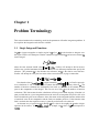
Chapter 1
Problem Terminology
This section introduces the terminology used for the parameters of PAR I NT integration problems. It
also explains the integration rules that are available.
1.1 Single Integrand Functions
Let be a hyper-rectangular or simplex region in
. Let
be the function to integrate over
the region. PAR I NT will attempt to calculate a numerical approximation and an error estimate
for the integral
where the error estimate should satisfy
. PAR I NT will attempt to find an answer
within a user specified maximum allowed error. There are two different parameters that specify this
tolerance. The parameter
is the absolute error tolerance and is the relative error tolerance.
PAR I NT will attempt to satisfy the least strict of these two tolerances, trying to ensure that:
Note that the value of
is approximated by
. As PAR I NT proceeds
in its calculations, it will, of course, need to evaluate the function
for many values of . The
number of function evaluations has traditionally been used as a measure of the amount of effort
spent in the computation of the integral. The user can set a limit
on the number of function
evaluations. This limit ensures that the calculations will not go on without stopping. Note that it is
quite possible that for a given integrand function, the result of an integration may not be able to be
achieved within the given error tolerances due to the nature of the integrand function and the effect
of round-off errors in the computation and the limits on machine precision. If the function count
limit is reached, then the required accuracy is generally not believed to be achieved.
An alternate way of specifying is through ; this value is the roughly the number of digits
requested in the answer. Or,
; for example, an
value of
corresponds to
.
2
Problem Terminology
There is also an alternate way of specifying . As the algorithm progresses, PAR I NT will
subdivide the initial integration region many times. It will evaluate each of these subregions. Instead
of limiting PAR I NT to some set number of function evaluations (via ), you can limit it to a
set number of region evaluations, via the corresponding
parameter. See Section 1.3 for more
information.
1.2 Vector Integrand Functions
The terminology presented in Section 1.1 actually represents a simplification of the problems capable of being solved. If there are several functions to be integrated over the same region, and they
behave similarly over that region (implying, of course, that they all have the same dimensionality),
then PAR I NT can integrate them together as a vector function.
The values , , and
are as before. With the integrand functions specified as
, PAR I NT
will calculate a numerical approximation to the integral
and an error estimate
while attempting to satisfy
where the infinity norm is used.
1.3 Integration Rules
There are several different kinds of integration techniques used in PAR I NT. The parallel integration
algorithm for globally adaptive cubature uses an adaptive subdivision technique at each processor,
where at each step the subregion with the largest error estimate is selected for subdivision. An
integral and error estimate is produced for the resulting parts using various integration rules. The
integral approximation is a linear combination of integrand values. The stochastic rules (MC and
QMC) rely upon applying a single “rule” of increasing accuracy to the entire integration region until
the desired accuracy is reached; also returning an integral and error estimate.
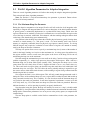
The integration rules are summarized in Table 1.1. Different integration rules work best for
(or are limited to) different kinds of functions, numbers of dimensions, or region types. This table
specifies the number of the rule (as it needs to be specified on the PAR I NT command line), the C
constant name for the rule (as is used in user applications), the type of region the rule supports,
and a description of the rule. The first four rules are from Genz and Malik [GM80, GM83], with
refined error estimation techniques from [BEG91]. The univariate rules are from the Quadpack
package [PdDÜK83]. The simplex rules are Grundman-Möller rules [Gen91, GM78]. The QuasiMonte Carlo rule uses a combination of Korobov and Richtmyer lattice rules [Gen98].
If you are integrating a single dimensional function, then select one of the univariate Quadpack
rules. If you have a 2 or 3 dimensional problem over a 2 or 3 dimensional hyper-rectangle, then
use Rule #1 or #2, respectively. For higher-dimensioned functions over a hyper-rectangle with a
1.3 Integration Rules
3
Rule#
1
C Constant
PI IRULE DIM2 DEG13
2
PI IRULE DIM3 DEG11
3
PI IRULE DEG9 OSCIL
4
PI IRULE DEG7
5
6
7
8
9
10
11
PI IRULE DQK15
PI IRULE DQK21
PI IRULE DQK31
PI IRULE DQK41
PI IRULE DQK51
PI IRULE DQK61
PI IRULE QMC
12
13
14
15
16
PI
PI
PI
PI
IRULE SIMPLEX
IRULE SIMPLEX
IRULE SIMPLEX
IRULE SIMPLEX
PI IRULE MC
DEG3
DEG5
DEG7
DEG9
Description
A 2-dimensional degree 13 rule for rectangular regions
that uses 65 evaluation points
A 3-dimensional degree 11 rule for hyper-rectangular
regions that uses 127 evaluation points
A degree 9 rule for -dimensional hyper-rectangular
regions, especially suited for oscillatory integrands.
A degree 7 rule for; the recommended general purpose
rule for -dimensional hyper-rectangular regions.
A univariate 15 point Gauss-Kronrod rule.
A univariate 21 point Gauss-Kronrod rule.
A univariate 31 point Gauss-Kronrod rule.
A univariate 41 point Gauss-Kronrod rule.
A univariate 51 point Gauss-Kronrod rule.
A univariate 61 point Gauss-Kronrod rule.
An -dimensional rule, using Korobov & Richtmyer
Quasi-Monte Carlo rules.
An -dimensional rule of degree 3 for simplex regions.
An -dimensional rule of degree 5 for simplex regions.
An -dimensional rule of degree 7 for simplex regions.
An -dimensional rule of degree 9 for simplex regions.
A simple Monte Carlo method.
Table 1.1: Integration rules used
moderate number of dimensions (e.g.,
), use Rules #3 or #4: Oscillatory functions generally
benefit from using Rule #3, whereas Rule #4 is a general purpose rule. (Note that Rules #3 and
#4 cannot integrate a univariate function.) If you have a simplex region, then choose one of the dimensional simplex rule. For functions of higher, even much higher (e.g., hundreds) dimensions,
use the QMC or MC rule.
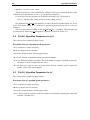
Rules #1 and #2 use a constant number of calls to the integrand function to calculate their result
and error estimate (using 65 and 127 points respectively). The number of function evaluations of
rules #3 and #4 and rules #12-#15 depend on the dimension of the problem, with higher dimensioned
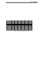
functions requiring more calls. Table 1.2 shows the number of function calls per evaluation of the
integration rule for these rules. From the chart it is apparent that for these rules, higher dimensioned
functions require much more time per rule evaluation. The QMC and MC rules are not applied
adaptively, so there is only a single rule “evaluation”, requiring a dynamically variable number of
function evaluations.
4
Problem Terminology
# Dimensions
2
3
4
5
6
7
8
9
10
Rule #3
33
77
153
273
453
717
1105
1689
2605
Rule #4
21
39
65
103
161
255
417
711
1265
Rule #12
10
17
26
37
50
65
82
101
122
Rule #13
16
27
41
58
78
101
127
156
188
Rule #14
26
47
76
114
162
221
292
376
474
Rule #15
41
82
146
240
372
551
787
1091
1475
Table 1.2: Function evaluations per rule evaluation
Chapter 2
Running PAR I NT from the Command
Line
Once a set of integration functions have been coded and compiled into a library of functions,
the easiest way to invoke PAR I NT is to call it at the command line. PAR I NT should work with
any version of MPI that adheres to the standard; it has been explicitly tested on MPICH [Cen95],
LAM / MPI [GLDS96, GL96], and MPICH - GM, the Myrinet adaptation of MPICH.
The parameters of the integration problem, such as the function to integrate, the region boundaries, the desired accuracy, etc., can be specified using command line parameters. The results are
printed to stdout. Multiple integrals can be computed by combining the commands that solve
them into a script. This section specifies the details of how to run PAR I NT from the command line.
2.1 Basics of the PAR I NT Executable
Note that a library of functions must be built before the PAR I NT executable can be used. This library
provides a method by which PAR I NT can call these functions internally when they are referred to
by name on the command line. The PAR I NT executable uses a run-time loading environment which
can load a PAR I NT Plug in Library (PPL) containing functions. The program is distributed with a
loadable module of sample functions called stdfunc.ppl. In the absence of command-line flags
indicating which library to load, the executable automatically loads the stdfunc.ppl library.
The library provides default values for , , an integration rule, and a function count limit for
each integrand function, as well as a default region over which to integrate. The integrand function
library makes it quick and easy to specify a function and parameters for an integration problem. The
details on integration function libraries are provided in Chapter 4.
Since PAR I NT 1.2 is written using the MPI message passing system, the mpirun command (or a
similar command) must be the actual command run. The details of how to use MPI are not examined
here, rather the user is referred to [GLS94]. The syntax and sample PAR I NT calls presented here
assume that the user is appending to them an mpirun command and its options. For example:
> mpirun -np 4 parint ...
6
Running PAR I NT from the Command Line
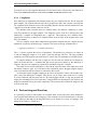
> parint [[-L ppl-name] -f fcn-name -h -i[1 2 3] ]
[-r rule] [-ea eps-a] [-er eps-r] [-ed eps-d]
[-lf fcn-count-limit] [-lr rgn-count-limit]
[-rgn rgn-specifier]
[-ohr help-ratio] [-ons ns] [-onr num-runs] [-ohs heap-size]
[-o optval]
Figure 2.1: Syntax of the PAR I NT executable
as might be used with MPICH. The output is sent to standard output, the errors to standard error, and
they may be redirected at the UNIX/Linux command line as desired. In PAR I NT 1.2, standard input
is not used.
The syntax of the PAR I NT call is presented in Figure 2.1.
Each option is specified by a parameter consisting of a “-” and a sequence of one or more letters.
Most parameters also require a value after the letters; a space may optionally appear between the
letters and the value, except as noted below.
There are two kinds of parameters that can be specified, integration parameters, which are the
parameters of the integration problem itself, and algorithm parameters, which modify the behavior
of the program as it calculates the integral. Generally, users do not need to modify or even know
about the algorithm parameters.
Each run of PAR I NT will evaluate the integral specified by the integration parameters. Any
option specified will override the corresponding value specified in the integration function library.
Algorithm parameters have a single default value used across all functions unless overridden.
2.2
PAR I NT Command-line Parameters
The following briefly describes each parameter:
-h Prints the usage of the PAR I NT command, with a brief explanation of each parameter.
-i, -i1, -i2, -i3 Prints out a list of the currently defined functions. The option -i1 prints
out a list of function names and descriptions (intended to be used by users to see what the
current functions are); the option -i2 is used internally by the GUI to get a more complete
listing of the function library and all default parameter values. If only -i is specified, then
the behavior is the same as -i1. The listing reflects the currently selected PPL library. The
option -i3 lists out all of the defined functions across all PPL files on the defined search
sequence for finding PPL files. This output is in the same format as -i2.
-L ppl-name The name of the PPL library to use. The executable searches for the library using the
search sequence described in Section 2.2.1 below.
-f fcn-name The name of the function. The name is case-sensitive and should match one of the
function names in the library of functions.
2.2 PAR I NT Command-line Parameters
7
-r rule The integration rule to use. Specify the rule with a value from 1 through 16, as explained
in Section 1.3.
-ea eps-a The value of the absolute error tolerance ( ). The value may be specified as a fixed or
floating point number, and must be greater than or equal to zero. (A zero value will effectively
result in only the eps-r/eps-d tolerance being used by PAR I NT.)
-er eps-r The value of the relative error tolerance ( ). The value may be specified as a fixed or
floating point number. Note that this value is dependent upon the machine architecture. The
value must be less than the corresponding machine precision, e.g., a common minimum eps-r
value when using the PAR I NT default precision is
. Note that this value is dependent
upon the machine architecture. If a zero value is specified, then only the eps-a parameter will
be used. At least one of eps-a and eps-r must be positive.
-ed eps-d The value of the relative error tolerance, specified as the number of digits of accuracy
( ). The value must be an integer, greater or equal to zero. This is simply an alternate way
of specifying eps-r; PAR I NT will convert the eps-d value into the equivalent eps-r value1
-lf fcn-count-limit The limit on the number of function evaluations to perform ( ). This value
counts the number of times the integrand function is called, and does not take into account
the number of functions in the vector of functions. The value must be greater than zero. The
maximum value of this parameter, as of PAR I NT 1.2, is the maximum value of an unsigned
long long int in C, or usually (depending upon the machine architecture)
2.
-lr rgn-count-limit The limit on the number of region evaluations to perform ( ). As each
region evaluation consists of a fixed, constant number of function evaluations (based on the
integration rule and function dimensionality), this is merely an alternate method for specifying
the -lf option. The value must be greater than zero, and as with , must be less than
approximately
(depending upon the machine architecture). This parameter can not be
specified if using one of the QMC or MC integration rules.
-rgn rgn-specifier The region over which to integrate. The integration rule being used determines
whether a simplex region or hyper-rectangular region is being used, and, determines the form
of the rgn-specifier. Hyper-rectangular regions are specified as
, and
simplex regions are specified as
. The values must be separated by white space. The -f option must be specified before the -rgn
option; as PAR I NT scans the command line parameters, it will therefore know the number of
dimensions for the region, and know how many values values to expect. The values may be
specified as fixed or floating point values.
1
PAR I NT will calculate
. Note that the numerical analysis community does not consider specifying,
of
, to be the same as requesting 3 digits of accuracy, so the value is not truly specifying that many
e.g., an
digits of accuracy.
2
Before PAR I NT 1.2, this value was limited to the size of a normal unsigned integer (
). Responding to user’s comments, we increased the size of this value, and all related values (all function counts, all region
counts, etc.) to be of this larger size, to handle the larger problems that are now being encountered.
8
Running PAR I NT from the Command Line
All of the -o and -oxx options set optional algorithm parameters that change the behavior of
PAR I NT. If they are not specified, then the compile-time default values for these will be used.
Mostly, users will not modify these values from their defaults. For more information on these
parameters, see Chapter 5.
2.2.1
PPL
search sequence
The command line may contain a fully qualified name to a PPL library or just a partial specification
to the library. The executable searches for a matching PPL library by automatically adding .ppl
to the file name if it is not already present and using the following sequence of steps (the example
assumes a command-line specification of -L stdfuncs). The first library found is used.
1. The library as named on the command line extended using .ppl:
./stdfuncs.ppl
2. The location specified by the environment variable PI PLUGIN DIR:
$PI PLUGIN DIR/stdfuncs.ppl
3. The library installation directory as specified at compile time using --prefix or the other
installation directory flags:
/usr/parint/lib/stdfuncs.ppl (Assuming installation into /usr/parint)
4. The standard system library location, /usr/lib:
/usr/lib/stdfuncs.ppl
If no PPL file is found, then an error results.
2.3 Restrictions on Parameters
The parameters can be specified in any order, with the following restrictions.
If -L is used, it must appear before -f or -i
Only one of -f, -h, or -i may be used, and each may only appear once.
If -i or -h is used, then all other options will be ignored.
If -f is used, then it must appear before the -rgn option.
If a parameter is used multiple times, specifying a different value each time, then the last
occurrence determines the value that will be used for the run.
Any of the -o or -oxx options may appear anywhere.
2.4 Sample PAR I NT Runs
9
2.4 Sample PAR I NT Runs
As previously noted, the mpirun part of the commands are removed from the following examples.
This example runs PAR I NT using a function named fcn7, using all the parameter values for fcn7
from the default integration function library:
> parint -f fcn7
This example runs the function fcn8i in the PPL library finance. Note: This library is not
part of the distribution — it is simply an example.
> parint -L finance -f fcn8i
This example also runs fcn7, but specifies a limit on the number of function evaluations and
an eps-r value. Note that the -f option does not need to be the first parameter; in general the
parameters can be specified in any order.
> parint -er1.0e-9 -lf1000000 -f fcn7
This example specifies the region over which to integrate. Note that fcn7 is a three-dimensional
function, and will be integrated over the three-dimensional cube of length 2.0 cornered at the origin:
> parint -f fcn7 -rgn 0.0 0.0 0.0 2.0 2.0 2.0
This example will print out a brief listing of the functions in the default integration library:
> parint -i
This example will print out a brief listing of the functions in the finance library
> parint -L finance -i
2.5 Interpreting the Results
This section presents a sample run along with the output. The run used is:
> parint -f fcn7
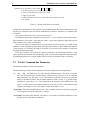
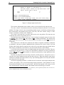
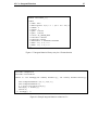
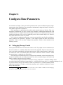
The output is given in Figure 2.2.
First, the integration parameters are printed. The values and the region boundaries are printed
to a number of digits corresponding to the precision used; this output results from a double precision run for a hyper-rectangular region. (PAR I NT has an installation option that allows for different
limits on the maximum precision allowed; see Section 6.4.) The region boundaries are printed in
rows three values across, up to the dimension of the region. Simplex regions are printed similarly.
Both the function count limit and the corresponding region count limits are printed, regardless of
whether -lf or -lr was specified.
10
Running PAR I NT from the Command Line
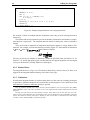
INTG PARMS: fcn7: f(x) = 1 / (x0 + x1 + x2)ˆ2
#Dims: 3; #Fcns: 1; Intg Rule: 4
Fcn Eval Limit: 400000 (== Rgn Eval Limit 10257)
eps-a: 1E-06; eps-r: 1E-06
A[]:
0
0
0
B[]:
1
1
1
RESULT: 0.863045354201518
ESTABS: 9.97673690990844E-07
STATUS: Fcn count: 33189; Rgn count: 851; Fcn count flag: 0
Time: 0.064; Time/1M: 1.91425
Figure 2.2: Sample output from PAR I NT
The result and estabs (error estimate) values are also printed based on the precision.
The “Fcn count” is the number of function evaluations performed by PAR I NT as it solved the
problem. The “Rgn count” is the corresponding number of region evaluations performed during
the execution (this is not printed if using a QMC or MC rule). The “Fcn count flag” is 1 if the
function count limit is reached, and is 0 otherwise.
The “Time” is the total time, in seconds, that it took to solve the problem. This time does not
include the time it takes to spawn the processes.
Note that if the region volume is zero (e.g., if, for some hyper-rectangular region, for some value
), then a result of
, with an error of
, is returned immediately. The function and
of ,
region count will be zero, and, in this case the execution is not timed, so a time of
seconds will
be reported.
The “Time/1M” is the total time, divided by the number of function evaluations, multiplied
by 1000000, or, the time to perform 1000000 function evaluations This value is useful; if you run
PAR I NT and it hits the function count limit, this value tells you an approximate upper bound on how
much longer it would take to run PAR I NT if you increase the limit by a certain amount.
It is possible for the function count to be slightly higher than the function count limit. There are
several reasons why this may be so. First of all, the function evaluations are always performed in
groups of
, where
is the number of evaluations performed by a single application of the
3
integration rule .
Secondly, the integration rules are being executed by all the processes. One process acts as a
controller and collects updated results from the other processes. When the function count limit is
reached, the controller tells all the workers to stop. Any remaining updates received by the controller
after that point will be discarded.
Note that an algorithm parameter is available that will execute the same integral multiple times
(via the -onr option). This is used when running timing experiments. If this parameter is used,
and specifies the number of runs to be greater than 1, then the time reported is the average over the
runs, and the function count flag printed is the number of times that the flag was reached.
3
Actually, they are performed in larger groups, as controlled by various algorithm parameters that control the frequency of update messages sent by the integration workers.
2.6 Practical Limits on PAR I NT
11
There is one fairly rare situation where the function count flag will be printed as a 1 even when
the limit was not reached. In this case, an unusual situation occurred internally, and the required
accuracy has most likely not been reached.
2.6 Practical Limits on PAR I NT
The behavior of PAR I NT depends greatly upon the platform on which it is run. This section attempts
to provide, however, a platform independent and simple guide to the practical limits of PAR I NT and
what behavior can generally be expected as these limits are reached.
When running PAR I NT on a new integrand function, you may first want to run it for fairly large
tolerances, for fairly low function count limits, in order to test it. As you decrease the allowed
tolerances, it is increasingly likely that the function count will be reached. If you truly want an
answer to the desired accuracy, you will need to increase the function count limit.
As PAR I NT attempts to find answers to smaller tolerances, it becomes more likely that roundoff errors will cause problems. As the PAR I NT algorithm proceeds, it necessarily has to sum up
many intermediate results. Each of these may introduce a small inaccuracy due to the limits of the
machine precision. As the number of region evaluations increases, these round-off errors may make
it impossible to reach the desired accuracy. A typical machine limit on the accuracy of double’s
is 15 digits, however, round-off errors may make it difficult to achieve greater than 12 or 13 digits
of precision in the integral approximation. Other integrand functions may require large amounts of
work to achieve much less precision; round-off errors may limit the result to that the precision.
In addition, PAR I NT dynamically allocates memory as it progresses. The higher the number of
iterations it uses, the greater the chance that it will not be able to allocate any additional memory
due to the limits of the hardware and operating system. In PAR I NT 1.2, if any process runs out of
memory, the entire run will be aborted. (See Section 5.3.1 for information on the -ohs parameters,
which can be used to avoid out-of-memory problems.)
As we will see in Chapter 3, PAR I NT can use either double’s or long double’s as a base
type for all floating point values. Using long double’s as the base type increases the accuracy
of the results, as well as the accuracy of all the intermediate results. This reduces the effect of
round-off errors, and as the precision on these values is much higher, you can expect to be able
to achieve more precise answers. However, the time to perform a single function evaluation can
increase greatly when using long double’s. And, as the time to perform a basic floating point
operation increases when using long double’s, you may find that the resulting time to solve the
integration problem has increased greatly.
The PAR I NT package is designed to operate in parallel in a distributed environment. The messages that are sent from one process to another during the progress of the algorithm introduce an
element of non-determinism: the computation of an integral, with a given set of integration parameters, always starts the same, but as some interprocess messages get sent quickly and others slowly
(due to the various demands upon the communication network) the progress of the algorithm can
begin to vary from one run to the next.
In practice, you will see that if you solve the same problem multiple times (using multiple processors), you will get slightly different results, also using different numbers of function evaluations.
This asynchronous behavior increases as the number of processors involved in the computation in-
12
Running PAR I NT from the Command Line
creases. If an integral is computed on a single workstation, there are no messages, and the algorithm
always progresses exactly the same way, yielding the same answer every time. This is, of course,
also seen with QMC or MC rules, where explicit pseudo-random numbers are used in the integration
process.
It can also take more function evaluations to solve a problem in parallel than on a single workstation. This is due to how the pieces of the problem are broken up and stored among the various
processors [ZdD00, Zan99]. In addition, it will generally take more function evaluations to solve a
problem as it as is solved on a greater number of processors. However, note that the problem will,
in general, be solved more quickly as more processors are involved, as each function evaluation is
effectively sped up.
2.7 Alternate Versions of PAR I NT
There are several different PAR I NT executables that come with PAR I NT 1.2. Each is suitable for use
in different situations.
2.7.1 General Purpose Versions of PAR I NT
The primary executable is the parallel MPI version, which has been introduced throughout this
chapter (parint).
The secondary executable is the sequential version. While it is possible to run the MPI version
of PAR I NT on a single processor, the reliance on MPI still introduces overhead into the executable
image and at run-time, and, obviously, requires some implementation of MPI to compile. The
sequential version of PAR I NT (sparint) compiles without any reliance on MPI. It can be run
from the Unix/Linux command line without relying on MPI to start processes. It is not as powerful
as the parallel version of PAR I NT, given that it is sequential, but can be useful when solving smaller
integration problems. In addition, the use of MPI often introduces delays in starting processes. The
sequential version of PAR I NT has no such delays; in solving problems that require little work, results
are available (in human terms) nearly instantaneously.
All of the integration parameters are the same for the sequential verison of PAR I NT, with correspondingly identical command line parameters. For example,
> sparint -f fcn7
will integrate fcn7 using the default parameters.
The algorithm parameters (as explained more fully in Chapter 5) are very different for the sequential version, as these parameters are used mostly to modify the parallel behavior of the algorithm. There are only two algorithm parameters that are used in the sequential version. First, the
“number of runs” parameter, specified using the -onr parameter on the command line. Secondly,
the “max heap size” parameter (see Section 5.3.1), specified using the -ohs option on the command
line. Note that logging (see Section 6.10) is not currently available in the sequential version.
2.7 Alternate Versions of PAR I NT
-L ppl-name
-f name
-r rel-error
-a abs-error
-l fcn-lim
-d n
-[
-h
]
13
External library of integrand functions
Integrand function name
Requested relative error
Requested absolute error
Function evaluation limit
Dimension (to be omitted if region is specified)
Hyper-rectangular integration region
This help
Table 2.1: QMC and MC executable command line options
2.7.2
QMC
and MC Versions of PAR I NT
There are stand-alone executables that can be compiled and executed separately from the main
PAR I NT code. The parallel executable names are pqmc and pmc, while the sequential executables
are sqmc and smc (for QMC and MC, respectively). (For details on the PAR I NT QMC algorithm,
see [Cd02].)
The command line options for all of these executables, although similar in functionality with
the ones described for the main code, presently have a different syntax, see Table 2.1.
These options do not accept spaces between the identifier and its value. For example, the following call will generate an error:
> pqmc -f mvt
The correct way is:
> pqmc -fmvt
Options are handled this way for all of the QMC and MC executables. See Sections 5.4 and 5.5
for information on the algorithm parameters for these executables. Note that you can select the QMC
and MC rules from the general purpose versions of PAR I NT. The only reason for these standalone
applications is to gain access to the QMC and MC specific algorithm parameters, which for this
release can only be accessed through these separate executables. Future releases will allow the
general purpose executables access to all parameters.
14
Running PAR I NT from the Command Line
Chapter 3
Running PAR I NT from a User
Application
In addition to the PAR I NT executable, PAR I NT can be used as a library of C functions (i.e., an
Application Programming Interface, or, API) which can be called from a user’s application program
to solve an integration problem. The user may find this to be more convenient, or, their application
may need to perform an integration step at some intermediate step of a larger calculation. To use
PAR I NT in this fashion, the user needs to be familiar with using MPI.
There are PAR I NT functions to initialize the PAR I NT environment, set parameters, solve problems, print results, and then finalize the run.
This chapter specifies how to use PAR I NT in this fashion, including explanations of some sample
code, details on all of the function in the API, and how to compile and link the resulting application
program. Note that the API only interfaces with the parallel version of PAR I NT, not the sequential
version of PAR I NT (i.e., sparint; see Section 2.7.1).
There are also functions for changing the algorithm parameters of PAR I NT. Most users will not
need to worry about these functions; they are presented in Chapter 5.
It is easiest to present a simple PAR I NT example of an application program before going into
any details. Consider the program presented in Figure 3.1. This example is an SPMD program; all
processes initiated by MPI will execute the same executable file (even though within the PAR I NT
functions there is separate code for processes that fill different roles in the calculation.)
The header file parint.h is included (Line 1 in Figure 3.1) to provide needed prototypes,
definitions, etc. C++ applications must have extern "C" directive as follow:
extern "C"
#include
parint.h
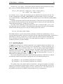
The function fcn7() (Line 5) is the C implementation of the integrand. For a given dimensional value, it will calculate the desired function value.
Inside main(), the function pi init mpi() is called (Line 20) to initialize the MPI and
PAR I NT environment. The function pi_allocate_hregion() allocates (Line 21) a data structure which will hold the region over which the function will be integrated; this structure is initialized
in lines 22-26. Then, pi_integrate() is called (Line 27) to actually perform the integration
16
1
2
3
4
5
6
7
8
9
10
11
12
13
14
15
16
17
18
19
20
21
22
23
24
25
26
27
28
29
30
31
32
33
34
35
Running PAR I NT from a User Application
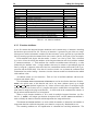
#include <parint.h>
#define DIMS
3
int fcn7(int *ndims, double x[], int *nfcns, double funvls[])
{
double z = x[0] + x[1] + x[2];
z *= z;
funvls[0] = (z != 0.0 ? 1.0 / z : 0.0);
return 0;
} /* fcn7() */
int main(int argc, char *argv[])
{
double result, estabs;
pi_status_t status;
pi_hregion_t *hrgn_p;
int nPE, rank, i;
pi_init_mpi(&argc, &argv, &rank, &nPE);
hrgn_p = pi_allocate_hregion(DIMS);
for (i = 0; i < DIMS; i++)
{
hrgn_p->a[i] = 0.0;
hrgn_p->b[i] = 1.0;
}
pi_integrate(fcn7, 1, PI_IRULE_DEG7, 400000, 1.0E-06, 1.0E-06,
hrgn_p, PI_RGN_HRECT, &result, &estabs, &status);
if (pi_controller(rank))
pi_print_results(&result, &estabs, 1, &status);
pi_free_hregion(hrgn_p);
pi_finalize();
exit(0);
} /* main() */
Figure 3.1: Simple PAR I NT application
3.1 Some PAR I NT Internals
17
problem. The parameters of this function specify the integration parameters for the problem ( , ,
the integration rule, etc.); the results of the integration are passed back via other parameters. Note
that fcn7() is passed in as a callback function to pi_integrate().
Once the pi_integrate() call has completed, the answer is available for printing or other
use. In this example, the function pi_print_results() is used (Line 30) to print the results.
The function pi_controller() (actually, it is a macro) is used as a guard (Line 29) to ensure
that only the controller process prints the result.
Finally, the function pi_free_hregion() frees the memory allocated by pi_allocate_hregion(),
and pi_finalize() closes the PAR I NT and MPI environment (Lines 32 and 33).
This sample application would need to be compiled and then linked with both the MPI library
and the PAR I NT library. For Monte Carlo integration rules the SPRNG library is required (see the
installation directions in Appendix A). At that point, the application could be run as an argument to
the mpirun command.
Although, the integration rules for QMC and MC involve completely different methods (from
both numerical and parallel point of view) than the adptive ones, it is completely transparent to
user application. At the present time, the user can not be specify QMC or MC algorithm specific
parameters in the user application.
3.1 Some PAR I NT Internals
Before presenting the PAR I NT functions, some of the PAR I NT internals need to be explained.
To use PAR I NT functions in a program, the PAR I NT C header file parint.h must be #include’ed
in the application program. This file is located in the $ PI HOME /include directory under the
main ParInt directory ($ PI HOME is the directory where PAR I NT was installed; see Appendix A).
It contains needed constants, type definitions, prototypes, and error codes that will be used by a
user’s application.
The most important of these definitions is the definition of the pi_base_t type. This type
is used within PAR I NT for any variable that represents a floating point value, including results,
error estimates, region boundaries, desired tolerances, etc. This type can either be the C data type
double or long double based on how PAR I NT was installed. (The default value is double,
for information on changing this and other compile-time values, see Chapter 6.)
A user’s application code does not need to use this type. If all of a user’s applications always
use, e.g., double’s, for floating point values, then all related variables inside the applications can
be of that type. Provided that PAR I NT is installed to use double’s, everything will work fine. Only
if the user wants to switch back and forth between the two types does pi_base_t need to be used.
Since values of type pi base t are passed to the integrand function, the type of the integrand
function actually changes as the pi base t type changes. This is discussed in Section 4.1.4.
3.2
PAR I NT Error Handling
There are several different types of problems that can occur while PAR I NT is running which will
cause execution to halt and an error message and error code to be returned. Some occur internally
and some are the result of errors in user programs. The error codes that can be returned are provided
18
Running PAR I NT from a User Application
as constants in the header file parint.h. If the PAR I NT executable is running, then the error code
is returned to the UNIX shell.
In addition, as most errors are not able to be recovered from easily, an error occurring in a
PAR I NT function called from a user application will also terminate the program and return an error
to the UNIX environment. Users are not able to, in general, catch error codes as return values from
PAR I NT functions.
Specifically, when an error is detected, a message is printed. Then, the entire MPI COMM WORLD
communicator is aborted (provided that the MPI environment has been initialized before the error
occurs) via an MPI Abort() call1 . Then, the standard POSIX call exit() is made with the
appropriate error value.
MPI is run internally with the default error handler, so that any MPI error that occurs will also
cause the entire process to abort. Below are some specific errors that can occur:
Calling sequence errors If the PAR I NT functions are called out of order in a user application (e.g.,
calling pi integrate() before pi init mpi()) then an error results.
Parameter errors This error occurs if a parameter passed to a PAR I NT function is invalid, or if a
command line argument to the PAR I NT executable is invalid.
Internal Errors There are a few internal errors that can conceivably occur while PAR I NT is running. For example, PAR I NT must dynamically allocate memory during execution; it is possible for PAR I NT to get an out of memory error.
Note that one error that could occur in PAR I NT 1.0, specifying the “wrong” number of processors, can no longer occur. PAR I NT 1.0 restricted the number of processes to being or
; this
restriction was removed for PAR I NT 1.1 and later releases.
3.3 The PAR I NT API Functions
This section presents the PAR I NT functions in detail. For each function, the syntax and parameters
are presented and the detailed use of the function is explained. (Note that there are also PAR I NT
API functions which modify algorithm parameters; most users willl not need to deal with these
functions. See Section 5 for details on them.)
3.3.1
PAR I NT Initialization
Before PAR I NT can be used to solve an integration problem, one of the PAR I NT initialization functions must be called. Internally, these functions initialize variables and perform some error checking
on the MPI environment.
There are two different initialization functions. They differ in whether the user or PAR I NT
initializes the MPI environment.
1
A design decision was made to halt the entire MPI COMM WORLD communicator, rather than the (potential subgroup
of) processes that PAR I NT is using, because MPI does not gracefully handle dying processes; if the PAR I NT execution
must be halted, then most likely the entire calculation will have to be aborted.
3.3 The PAR I NT API Functions
19
The first is pi_init_mpi(). This function will first initialize the MPI environment (by calling
MPI_Init()), and then initialize the PAR I NT run. The syntax is as follows:
int pi_init_mpi(int *argc_ptr, char **argv_ptr[],
int *rank, int *comm_size);
As with MPI_Init(), argc_ptr and argv_ptr are initialized and returned to the user. The
sole MPI communicator used is MPI_COMM_WORLD; the rank and comm_size are set to the process’es rank within MPI_COMM_WORLD, and, the size (number of processes) within MPI_COMM_WORLD,
respectively.
If MPI has already been initialized when this function is called, then an error will be reported.
Since PAR I NT does the initializing of MPI when this function is called, it will also do the finalizing
of MPI when the function pi_finalize() is called.
The other PAR I NT initializing function requires the user to perform the MPI_Init() call.
This allows the user to, for example, divide the default world group of MPI into several subgroups
and then run the PAR I NT processes in only one of those groups. The syntax is:
int pi_init(MPI_Comm comm);
The comm parameter is passed to the function indicating to PAR I NT the communicator to use to
solve the integration problem. At the end of execution, the user’s application should call MPI_Finalize(),
either before or after pi_finalize() is called. If MPI has not been initialized when this function is called, then an error will be reported. The sample application sample2.c, provided in the
installation of PAR I NT, uses this technique.
3.3.2 Initializing Regions
The -dimensional region over which the integration is to be completed must be specified for every
integration problem. This region is passed in to pi_integrate() via the pi_hregion_t or
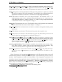
pi sregion t structure, as defined in Figure 3.2. These are used to specify hyper-rectangular
or simplex regions, respectively. Each each structure, the ndims field specifies the number of
dimensions for the region. In pi hregion t, the a[] and b[] vectors specify the lower and
upper integration limits of the region. In pi sregion t, the vertices field is set up as a 2
dimensional array holding the simplex’s coordinates.
The vectors holding the region values must be allocated dynamically. While the user could do
this manually, functions are provided to automate this task. The function prototypes are:
pi_hregion_t *pi_allocate_hregion(int ndims);
pi_sregion_t *pi_allocate_sregion(int ndims);
The ndims value is the desired number of dimensions. For hyper-rectangular and simplex
regions, the corresponding function returns a pointer to a freshly allocated structure of the corresponding type of region, containing pointers to array(s) of the given size. The returned pointer to
the structure can be stored in a suitable variable and passed to pi_integrate().
20
Running PAR I NT from a User Application
typedef struct {
pi_base_t *a;
pi_base_t *b;
int
ndims;
} pi_hregion_t;
typedef struct {
pi_base_t **vertices;
int
ndims;
} pi_sregion_t;
Figure 3.2: Structure definitions for the pi hregion t and pi sregion t types
PAR I NT 1.2 can support integration over regions of any number of dimensions. The only error
that can occur is from the C function malloc(), possibly an E_NO_MEM (the Unix out-of-memory
error; see errno.h) error if there is no more memory for allocation. As noted in Section 3.2, any
error will cause an abort of the entire run, so it is not necessary to include code that will check
for an error value returned from the function. Note that this function can be called before any
PAR I NT initialization function (or even after pi_finalize() is called, though that would serve
no purpose).
After the problem is solved by pi_integrate(), and the region is no longer needed, the
memory allocated for the region needs to be freed. This can be done with one of the functions:
void pi_free_hregion(pi_hregion_t *hregion_p);
void pi_free_sregion(pi_sregion_t *sregion_p);
Use the freeing function corresponding to the allocation function used. The pointer passed in should
be the pointer value originally returned by the allocatioon function. The only error possible is a
PI_ERR_PARMS error if the given pointer parameter is NULL. Results are undefined if an invalid
(but non-NULL) pointer is passed in.
3.3.3 Executing the Integration
Once PAR I NT has been initialized and the region has been defined, the integration can be completed.
The function pi_integrate() performs that task. The prototype is as follows:
int pi_integrate(pi_ifcn_t ifcn_p, int nfcns, int intg_rule,
pi_total_t fcn_eval_limit, pi_base_t eps_a,
pi_base_t eps_r, void *region_p, int region_type,
pi_base_t result[], pi_base_t estabs[],
pi_status_t *status_p);
The result[], estabs[], and status_p parameters contain values set by the function
call, all other parameters contain input values for the function. The parameters intg rule,
3.3 The PAR I NT API Functions
21
fcn eval limit, eps a, and eps r all directly correspond to parameters of the PAR I NT executable, and, except as noted, have the same requirements for their values. (The type pi total t
is typedef’ed to be a long long int.) The parameter descriptions are as follows:
ifcn p The pointer to the integrand function. The type of this parameter is a pointer to a function
that returns an integer and has the parameters corresponding to the integrand function as
implemented in PAR I NT (see Section 4.1 for details on coding integrand functions).
nfcns The number of functions in the vector integrand function. The minimum value is 1, the
default maximum value is 10 (as defined in the header file parint.h). A non-vector (i.e.,
scalar) integrand function is treated by PAR I NT as a vector of a single component function,
so the nfcns value for a scalar integrand is simply 1.
intg rule The integration rule to use. The allowable values for this parameter are enumerated
in the PAR I NT header file, and are listed in Figure 1.1 on Page 3.
fcn eval limit The maximum number of function evaluations the algorithm should perform
during a run.
eps a The absolute error tolerance. The value must be greater than or equal to zero.
eps r The relative error tolerance. The value must be greater than the machine precision for the
given PAR I NT base type being used, as explained in Section 2.2.
region p and region type The region p pointer should be a pointer to a structure of type
pi hregion t or pi sregion t which has been properly allocated and filled in with the
region’s boundaries. The region type should be the constant PI RGN HRECT if using a
hyper-rectangular region, or PI RGN SIMPLEX if using a simplex region.
result[] and estabs[] These parameters contain the answer and the error estimate, respectively. They are arrays, with one value for each of the nfcns in the vector function. They
should be declared by the user’s application code to be of the appropriate size.
status p A pointer to a user-declared structure of type pi status t. The fields in this structure will be set by pi integrate() to reflect the integration run. For details see Section 3.3.4.
Since all processes will execute the pi integrate() call, all processes have access to all
of the function parameters, including the function pointer. Note also that all processes will synchronize2 before beginning to actually solve the problem. If the integration is performed as an
intermediate step in a large application, then the integration will not commence until all processes
participating in the integration call pi integrate(). When the pi integrate() function
finishes, only the controller process (as determined by the pi controller() function) will
have the result, estabs, and *status_p values.
The function pi integrate() can result in the following errors:
2
Using an MPI Barrier() call.
22
Running PAR I NT from a User Application
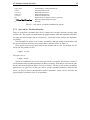
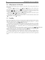
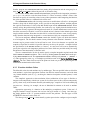
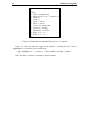
RESULT: 0.863045354201517
ESTABS: 9.98E-07 (Relative Error 1.16E-06)
STATUS: Fcn count: 33189; Region count: 851; Fcn count flag: 0
Time: 0.092; Time/1M: 2.77643; Time/Region: 1.08E-4
Figure 3.3: Sample results as printed by pi print results().
PI ERR FN ORDER Results if the PAR I NT functions are called out of order.
PI ERR PARMS Results if any of the parameters are invalid.
PI ERR INTERNAL Results if any miscellaneous error happens during the run, for example, a
memory allocation error.
3.3.4 Using the Results
Once pi integrate() has finished, the results are available for printing or for use by later
steps in the user’s application. It is important to note that only the controller process finishes the
integration with the results. If the other processes wish to use the results, they will have to be
broadcast or sent to them by the controlling process.
The function pi controller() can be used to determine which process is the controller. It
is actually a macro; passing in to it the rank of the process will yield a true result (i.e., the value 1)
when called by the controller, false (the value 0) otherwise, as in the following piece of code from
the sample application of Figure 3.13 .
if (pi_controller(rank))
pi_print_results(&result, &estabs, 1, &status);
In this piece of code, the function pi print results() is used to print the results. Its prototype
is as follows:
void pi_print_results(const pi_base_t result[], const pi_base_t estabs[],
int nfcns, const pi_status_t *status_p);
The result[], estabs[], and status p parameters should contain the values returned
by the integration step. The value nfcns is, as for pi integrate(), the number of functions in
the vector integrand.
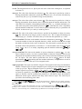
Figure 3.3 presents sample output from this function, corresponding to a run of the sample
application in Figure 3.1.
The function integrated is the same as the function fcn7 in the sample library of functions
, integrated over the standard 3 dimensional unit
provided with PAR I NT, or,
cube (cornered at the origin).
3
The controller process is just the process with the rank of zero in its group (i.e., its MPI communicator). However, the
macro pi controller() is provided in this release to ensure compatibility with future releases where the controller
may be an arbitrarily ranked process.
3.3 The PAR I NT API Functions
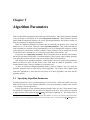
typedef struct
double
pi_total_t
int
int
} pi_status_t;
23
{
total_time;
fcn_eval_count;
fcn_limit_flag;
fcn_evals_per_rule;
Figure 3.4: Structure definition for the pi status t type
The print function prints out one result and error estimate for each of the functions in the vector
of functions; in this example, there is only a single function. Each result is printed to the maximum
number of digits available, based on the (machine) precision used. Each absolute and relative error
estimate is printed to a default of 3 digits4 .
In addition, information about the integration run is provided. This information is found in the
status p parameter. This parameter is a pointer to a structure of type pi status t, shown in
Figure 3.4.
The total time field contains the time it took to complete the integral, measured in seconds
and fractions of a second (as is returned internally by MPI Time()). Note that the timer is started
and stopped within pi integrate(), so neither the MPI process spawning time, nor the PAR I NT
initialization time, is included in this value.
The fcn eval count represents the number of times the integrand function was evaluated
by PAR I NT. The fcn limit flag has a value of 1 if PAR I NT evaluated the function more
than the function count limit, or 0 otherwise. These values mirror the values printed out when
running the PAR I NT executable; see Section 2.5 for details on these output values. The field
fcn evals per rule stores the number of function evaluations per rule evaluation (as specified in Section 1.3); this value can be used to calculate the region evaluation count.
Note that the total time divided by the number of function evaluations, times 1000000, is also
printed as the Time/1M value. This provides the user with a guide as to the time it would take to
complete the problem if the function count limit were to be increased.
3.3.5 Terminating the Process
Before the application is allowed to terminate, the function pi finalize() should be called. Its
prototype is:
int pi_finalize(void);
This function will call MPI Finalize() only if pi init mpi() was used to initialize
PAR I NT; if PAR I NT was initialized by pi init(), then the user must call MPI Finalize(),
either before or after pi finalize().
4
This constant is the CPP constant PI ESTABS DIGITS in $ PI HOME /include/parint.h. This value cannot yet be changed via the installation time configure script.
24
Running PAR I NT from a User Application
3.4 Calling Sequence for Functions
Some of the PAR I NT functions must be called in a certain order. This section provides details on
this ordering.
The functions pi controller() and pi allocate hregion() can be called at any
time (though it only makes sense to call pi controller() when the process’s rank is known).
The function pi free hregion() can be called any time there is a valid region structure to free
(but make sure that the structure is valid when pi integrate() is called).
The function pi print results() can be called any time there are valid results to print
(usually, of course, after pi integrate() has completed).
The primary PAR I NT functions must be called in order: a PAR I NT initialization function, then
pi integrate(), then pi finalize().
3.5 Compiling
Before the user application can be run, it of course must be compiled and linked with the PAR I NT
object code. This object code is compiled at installation time and from it a library (i.e., a .a file) is
created. This library resides in the $ PI HOME /lib directory.
The makefile for the user application must therefore specify where this library is to be found,
along with its name (libParInt.a). In addition, if the PAR I NT header file is included in the
source using angle brackets (i.e., “#include <parint.h>”), then the makefile must specify
where to find the header file.
The sample makefile that comes with the sample user applications (found in the $ PI HOME /samp-apps
directory performs these tasks. This makefile relies upon the PI HOME environment variable that
should be set up automatically by the configure script at installation time.
To modify the makefile for your own applications, change the variables accordingly (The automatic settings should usually be fine). Then, replace the names of the sample application source
file, object file, and, executable file with the appropriate file names based on the user application
names.
Chapter 4
Adding New Integrands
This chapter specifies how new integrand functions are added to the function library, both when
using the executable and in a user application. This section focuses on integrand functions written in C; Sections 4.4 and 4.5 explain how to use integrand functions written in Fortran and c++,
respectively.
4.1 The Integrand Function
Figure 4.1 shows a sample integrand function. This function was previously given in Figure 3.1. It
returns the value of
for a given 3-dimensional value).
The integrand function is called by PAR I NT many times during the computation of an integral.
Each time, the appropriate value is passed to the function, and the function is expected to calculate
and return in a parameter the appropriate
value.
4.1.1 Parameters
The x[] array in Figure 4.1 contains the -dimensional value for which the function calculates
the integrand component values. The values are stored in x[0], x[1], . . . .
The function result is stored in the funvls[] (short for “function values”) parameter. If the
integrand is only a single function, then the integrand value should be stored in funvls[0], as in
int fcn7(int *ndims, double x[], int *nfcns, double funvls[])
{
double z = x[0] + x[1] + x[2];
z *= z;
funvls[0] = (z != 0.0 ? 1.0 / z : 0.0);
return 0;
} /* fcn7() */
Figure 4.1: Sample integrand function
26
Adding New Integrands
int fcn7_star(int *ndims, double x[], int *nfcns, double funvls[])
{
double z = 0.0;
int i;
for (i = 0; i < *ndims; ++i)
z += x[i];
z *= z;
funvls[0] = (z != 0.0 ? 1.0 / z : 0.0);
return 0;
} /* fcn7_star() */
Figure 4.2: Sample integrand function with varying dimensions
this example. If there are multiple function component values, they go in the ensuing positions in
funvls[].
The ndims and nfcns parameters provide the number of dimensions and number of component functions, respectively1 . The integrand function should not change the values of ndims or
nfcns.
They can be used to implement an integration function that supports a varying number of dimensions. For example, consider the function specified in Figure 4.2. If the number of dimensions
is , for an value of
, this function calculates
The user can specify any number of dimensions (within the allowable limits for PAR I NT 1.2; see
Section 3.3.3), and an appropriate region, and this function will support integration over that region
(as long as the function is suitably defined over that region).
4.1.2 Return Values
The integrand function is of type int. The function should always return a value of 0. There is no
support for the integrand function returning error codes of any type2 .
4.1.3 Limitations
Given that the integrand function is evaluated many times over the course of evaluating an integral,
it represents a significant amount of the execution time for the integration. Users should try to write
their function to execute as efficiently quickly as possible.
1
They are parameters primarily due to legacy Fortran code that implements some of the integration rules [GM80,
GM83, PdDÜK83, Gen91]. Since they are pointers to int’s, they support Fortran’s implicit call-by-reference function
parameters.
2
Currently, the return value is not used by PAR I NT. However, future releases may use this value as an error code,
where a non-zero return will indicate an error. Returning a value of 0 now will therefore ensure compatibility with future
releases. Note that this is a change with respect to PAR I NT 1.0, where a return value of 1 indicated no error. This change
was made to reflect standard POSIX system call return values.
4.1 The Integrand Function
27
It is possible to add print statements to the function to debug its operation (provided that the
implementation of MPI being used supports output). Of course, they should be removed when the
code operates correctly. The function should not try to read any input from the user.
The user should be careful to avoid any floating point errors, e.g., divide by zero exceptions.
Consider, when writing a function, the regions over which it is to be integrated (as this determines
the range of values that will be passed to the integrand function).
The function in Figure 4.1 contains a method for dealing with the divide-by-zero problem.
is passed to
This function is undefined at the origin. Accordingly, when an value of
this function, is does not perform its usual calculation, rather, it just returns a zero. In this case,
“ignoring” the singularity leads to an area around the origin where the function is set to zero3 .
Since the “width” of the slice at which the function value is discontinuous is zero, the value of
the integral is not changed by this special case. At any other value of , the function is defined, and
the usual calculation is performed. This same technique is used in Figure 4.2.
While PAR I NT is implemented as a parallel program, the PAR I NT 1.2 code is not multi-threaded.
It is therefore possible to store “state” information, in the form of static variables, within the
function.
Consider the example presented in Figure 4.3. The function calculated here is
, where
and
. In this function, the intermediate values and are used in
calculating the integrand value. However, these intermediate values are calculated constants. You
would not want to have to calculate these values every time the function is called. You would also
prefer not to hardcode them as literal constants, in order to best handle varying machine precision.
So, the code in Figure 4.3 uses a static flag variable to determine whether or not the function
is being called for the first time. If it is, it calculates alpha and beta. Otherwise, it uses the
previously calculated values.
Note that implementing this function in a user application would be simpler. The alpha and
beta parameters could be global variables, accessible to the code that implements the integrand
function. They could be calculated once, before the pi integrate() function is ever called,
ensuring that they hold valid values whenever the integrand function is called.
4.1.4 The PAR I NT Base Type and Integrand Functions
The PAR I NT base type, pi base t, was introduced in Section 3.1. It allows for support of either
double (the default type) or long double integration results.
The integration function will normally be written to support only the installed value of pi base t.
The x[] and funvls[] parameters of the integrand function, as well as any appropriate local variables, should be typed either double or long double.
If users want to write a function that supports either type, then they should use the pi base t
type itself within the function. (Note that all functions in the provided default function library have
this support.) Figure 4.4 repeats the definition of fcn7(), but with this support.
3
Since this area is centered at zero, its size is determined by the underflow number. At a point different from the origin,
how close we can get to the singularity will depend on the machine precision. Thus even if “ignoring” the singularity is
justified theoretically, its implementation may result in discarding a significant portion of the integral. Further numerical
problems may be introduced in view of large values returned clsoe to the singularity. In some cases it may be desirable
to artifically increase the distance of evaluation points from the singularity.
28
Adding New Integrands
int fcn7_state(int *ndims, double x[], int *nfcns, double funvls[])
{
static int flag = 0;
static double alpha, beta;
if (!flag)
{
alpha = sqrt(1.2);
beta = sqrt(1.4);
flag = 1;
}
funvls[0] = pow(x[0], alpha) + pow(x[1], beta);
return 0;
} /* fcn7_state() */
Figure 4.3: Sample integrand function with state information
int fcn7(int *ndims, pi_base_t x[], int *nfcns, pi_base_t funvls[])
{
pi_base_t z = x[0] + x[1] + x[2];
z *= z;
funvls[0] = (z != 0.0 ? 1.0 / z : 0.0);
return 0;
} /* fcn7() */
Figure 4.4: Integrand function with support for pi base t
4.2 Integrand Functions Within User Applications
29
There are several problems which complicate support for pi base t in integrand functions.
These complications involve the use of C math functions and the specification of constants. For
details, see Appendix C.
4.2 Integrand Functions Within User Applications
When PAR I NT is used as a package of functions, called from a user’s application, then the integrand
function is simply specified with the user’s application source code.
The function is referenced by PAR I NT via the pointer to the function as passed to pi integrate().
4.3 Integrand Functions in the Function Library
When PAR I NT is used as a stand-alone executable, it uses the PAR I NT Plug in Library (PPL) mechanism to locate integrand functions. These functions are written by the user, added to the library
(along with some related information), and then compiled using a special compiler into plug-in
modules (.ppl files). A single PPL file is loaded at runtime by the PAR I NT executable. Using a
function library allows for quick access to a predefined set of functions and allows PAR I NT users
to dynamically add and remove integrand functions without re-compiling the PAR I NT binary. Once
these functions are stored in the library, they can be chosen for integration by name.
The PAR I NT program comes with a default PPL file which is automatically compiled and used
by the executable when the user does not specify an alternate PPL file.
This section explains the details of adding functions to a PPL file. The examples used are based
on the sample integrand library that comes with PAR I NT, found under the installation directory in
the src/pipic directory in the stdfuncs.c file.
4.3.1 Writing the Function
The actual integrand function is written the same as when writing a user application. The parameters, return value, and behavior are the same. The major difference between the two forms of function is that certain system calls are not allowed within PPL files. The list of disallowed system calls
is: accept(), bind(), fopen(), getmsg(), msgget(), open(), pause(), poll(),
putmsg(), select(), semop(), wait(), alarm(), brk(), chdir(), dlclose(),
dlerror(), dlopen(), dlsym(), exec(), fork(), popen(), pthread create(),
sbrk(), sethostent(), setgid(), setuid(), signal(), system(), thr create()
and umask().
In general, there will be more than one function in a single PPL file. These functions can be
written within a single source file or can be spread across several files. Due to the structure of
the compilation mechanism, all attribute blocks (see Section 4.3.2) must be defined within a single
source code file.
30
Adding New Integrands
Attribute
NAME
FUNCTION
NDIMS
NFCNS
DESCRIPTION
EPSA
EPSR
IRULE
FCNLIMIT
DEFANSWER
DEFA
DEFB
DEFSIMPLEX
Description
The name of the function.
Function identifier.
Number of dimensions.
Number of functions.
Function description for help information.
Default eps-a parameter value for the function.
Default eps-r parameter value for the function.
Default integration rule (rule) for the function.
Default fcn-count-limit value for the function.
Known answer (used for testing).
Default integration region minimum bounds.
Default integration region maximum bounds.
Default integration region for a simplex region
Default
Required
value of NAME
1
1
None
1.0E-06
1.0E-06
PI IRULE DEG7
400,000
0.0
0.0
1.0
None
Table 4.1: PPL function attributes
4.3.2 Function Attributes
A PPL file contains the integrand function definitions and a constant array of structures describing
the functions present in the PPL file. The array of structures is generated as part of the PPL compilation process and the information contained in these structures can be specified on a per-function
basis by inserting specialized comment blocks into a source code file. See Figure 4.5 for an example.
Each comment block begins with the marker “/*PPC*” on a line by itself. This is followed
by a series of lines describing the attributes of the integrand function and closed with the standard
C comment terminator */. Each attribute line contains an attribute name followed by a colon
followed by the attribute value. A single attribute value may be written to span multiple physical
lines by using the \ character at the end of the line (a mechanism similar to that used by the C preprocessor and the UNIX shell). Note that it is incorrect in this case to format the comment block
continuation lines with a leading * character, since the character would be included into the middle
of the attribute value.
All attribute names are case-insensitive. Table 4.1 lists all available attributes with short descriptions and default values.
The fields NAME, FUNCTION, NDIMS and NFCNS are used to describe the function to PAR I NT.
NAME is the public name of the function and can be any name (without spaces) up to length
PI MAX IFCN NAME (defined in parint.h). It does not necessarily have to correspond to the
function identifier, but in most cases it is simpler and easier to establish this correspondence. This
name must be unique to the plug-in and PAR I NT— it will be used on the command line with the -f
flag to indicate which function is to be integrated.
When a single function definition is to be used for multiple integrand functions (see Section 4.1.1), NAME is still unique per function description block, and the FUNCTION attribute is
used to identify the function identifier which implements the integrand function.
The NDIMS and NFCNS attributes are used to hold the number of dimensions and number of
component functions within the integrand vector function, respectively. Both default to one.
The remaining attributes are for simplification of command lines and help information. The
4.3 Integrand Functions in the Function Library
31
PAR I NT program uses DESCRIPTION when printing help information and the string may be at
most PI MAX IFCN DESC (defined in parint.h) characters long.
The attributes EPSA, EPSR, IRULE and FCNLIMIT correspond to the integration parameters
eps-a, eps-r, rule, and fcn-count-limit from Section 2.2. These are merely “default” values; if the
user does not specify an overriding value for one of these parameters when integrating the function,
the value specified in the PPC comment block will be used.
The DEFANSWER attribute aids in testing extensions or modifications to PAR I NT. An integrand
function, along with its default region, exactly specifies an integration problem, and that problem
has a specific actual answer. It is this value that should be put into the DEFANSWER attribute. When
actually solving the problem using PAR I NT, the results may vary slightly from the default answer,
based on the accuracy requested, the integration rule used, etc., but the default answer can be used to
check the correctness of PAR I NT’s result. If no default answer is known for the default region, then
simply omit this attribute. Note that since this field is a scalar field, and not a vector, it only properly
works when the function being integrated is a vector function of only one component function.
The last two attributes, DEFA and DEFB, contain the “default” region over which the function
is to be integrated. The list should contain as many elements as the function’s dimension - excess
elements may be present on the list but will not be used. If too few elements are specified, the
compiler will pad the list with 0.0 if possible (this may not always be possible - examples include
the specification of the NDIMS attribute as a macro). As most users will want to dynamically
specify the region for each integration problem solved, these fields are provided mainly for testing
the function or the functionality of PAR I NT itself.
The PPC comment blocks can also be used to specify a simplex integration region instead of the
default DEFA and DEFB formulation. This is done by omitting DEFA and DEFB and instead specifying DEFSIMPLEX instead. The DEFSIMPLEX attribute should specify NDIMS * (NDIMS +
1) values grouped by point (e.g., a 3D simplex specification needs to list
. The list is much easier to read if the points are listed one per line of input using the line
continuation mechanism described earlier.
4.3.3 Function Attribute Values
The allowable values for each attribute vary by attribute type. The text specified in the PPC block for
each attribute is copied into appropriate locations into PAR I NT internal structures, and aside from
very limited additions (such as, e.g., enclosing the function description in double quotes) is used
verbatim.
This simplistic approach to value translation allows redefinition of base types in PAR I NT to
integrate semi-transparently with the PPL system. It also allows users of this system to transparently
specify values in any of the formats allowed by the underlying C compiler as well as the underlying
pre-processor - allowing, for example, the use of #define’d constants to be used as attribute
values.
Appropriate typecasting is a function of the underlying compilation system. If the user’s C
compiler translates integer constants into an int data type instead of a long int data type,
the simple addition of the “l” constant modifier resolves the problem. The data types of each
ATTRIBUTE value are listed in Table 4.2.
The data type of pi base t is determined by options passed to the configure script at compile
32
Adding New Integrands
Attribute
NAME
FUNCTION
NDIMS
NFCNS
DESCRIPTION
EPSA
EPSR
IRULE
FCNLIMIT
DEFANSWER
DEFA
DEFB
DEFSIMPLEX
Type
char[PI MAX IFCN NAME + 1]
pi ifcn t
int
int
char[PI MAX IFCN DESC + 1]
pi base t
pi base t
int
long long int
pi base t
pi base t * (Treated as an array)
pi base t * (Treated as an array)
pi base t * (Treated as an array)
Transformation
Add double quotes
None
None
None
Add double quotes
None
None
None
None
None
None
None
None
Table 4.2: PPL attribute types
/*PPC*
* name: fcn7
* description: f(x) = 1 / (x0 + x1 + x2)ˆ2
* ndims: 3
* nfcns: 1
* epsa: 1.0E-06
* epsr: 1.0E-06
* irule: PI_IRULE_DEG7
* fcnlimit: 400000
* defanswer: 0.8630462173553432
* defa: 0.0, 0.0, 0.0
* defb: 1.0, 1.0, 1.0
*/
Figure 4.5: Sample PPC comment block for fcn7.
type. The two options currently supported are either double or long double. There are a series of
constant values and macro definitions available to integrand function implementors in pi-math.h
which change precision according to the selection of doubles or long doubles. Any of the constant
values defined in this manner may be used when specifying attribute values (see Appendix C).
Figure 4.5 shows a sample PPC comment block for fcn7, used elsewhere throughout this manual.
The name of the corresponding C function is simply fcn7. The default answer, approximately
, is the answer when this function is integrated over the default region, the standard three
dimensional unit cube. The default integration rule is specified using one of the constants defined
in the header file parint.h.
In Section 4.1.1 an integrand function fcn7 star() was presented (in Figure 4.2) that integrated a function for a variable number of dimensions. Such functions can be used in an integrand
function library. However, each entry in the library must have a single, specific number of dimensions, as provided by the ndims field. Therefore, to use such a function, multiple PPC blocks must
4.4 Fortran Integrand Functions
33
be created, one for each supported dimension. Each of these blocks will have the same function id
listed in the FUNCTION attribute with a different NAME and NDIMS attribute values.
4.3.4 Compilation
Once functions are augmented with attribute blocks, they are compiled into PPL files by using the
ppc compiler. The compiler behaves more like a pre-processor than a full compiler, extracting the
PPC comment blocks from the source code and adding PAR I NT internal structure definitions to the
.ppl file based on the contents of the PPC blocks.
The attribute values extracted from PPC comment blocks are added to a temporary C source
code file generated by the ppc compiler. This temporary source code file is then passed to the
underlying C compiler for compilation into a .ppl file. This temporary file is marked with C
preprocessor directives so that most C compilers report errors in terms of the original source code
file’s line numbers.
The PPC compiler accepts three command line parameters interpreted by the compiler and any
parameters accepted by the underlying C compiler. The syntax of the ppc command line is:
> ppc ppc-parameters -- C-compiler-parameters
The -- is used to separate the two sets of parameters. The optional ppc-parameters are either -d
to turn on debugging output or -h to print a short help message and exit. The only parameter
commonly used and required is the name of the C source code file containing PPC attribute blocks.
To compile multiple code files into a single PPL file, the code files which do not contain PPC
blocks are listed after the -- command line flag and are processed entirely by the underlying C
compiler. They may be compiled as separate files and linked using the C compiler.
The result of a successful compilation is a file with the same base name as the input source code
file and the extension .ppl. As a side effect of the compilation process the ppc compiler displays
a list of all functions and descriptions as contained in the PPL file.
As mentioned earlier, the ppc compiler pre-processes the original C source code and then compiles it using the underlying C compiler. This process can go wrong, and in such cases it is useful
to see the command and post-processed file. By invoking ppc with the -v flag, the program will
display the command line used to invoke the C compiler and leave the temporary file (listed on the
displayed command line) in place after compilation. The user may then examine the temporary file
to discover the error.
4.4 Fortran Integrand Functions
It is generally possible to link together an executable from several object files which themselves
were compiled from different source languages. This technique can be used with PAR I NT, allowing
for the functions that make up the integration library to be written in a variety of languages, even
though all of PAR I NT is written in C4 .
4
Though, some of the PAR I NT code was originally written in Fortran 77 and was converted to C code.
34
Adding New Integrands
INTEGER FUNCTION FCN20(NDIMS, X, NFCNS, FUNVLS)
INTEGER NDIMS, NFCNS
DOUBLE PRECISION X(*), FUNVLS(*)
DOUBLE PRECISION Z
Z = (X(1) + X(2) + X(3)) ** 2
IF (Z .NE. 0.0) THEN
FUNVLS(1) = 1.0 / Z
ELSE
FUNVLS(1) = 0.0
ENDIF
FCN20 = 0
RETURN
END
Figure 4.6: Sample integrand function written in Fortran
Figure 4.6 shows a sample integrand function written in Fortran. (Note that this is the same as
the function fcn7 used throughout the manual, but is written in Fortran.) The following makefile
fragment will compile the source file (a file named fcn20.f) into an object file:
fcn20.o : fcn20.f
${F77} -c fcn20.f
Figure 4.7 shows the input file to ppc for this function. The file starts with a declaration of the
Fortran function. Note that the function was written as “FCN20” but is specified in the library as
“fcn20 ”. The name changes (the capitalization change and the trailing underscore) are generally
system dependent, and reflect the difference between named objects in C and Fortran.
Next comes the PPC comment block in exactly the same format as was used earlier in Figure 4.5
with the addition of the FUNCTION attribute naming the external Fortran function name.
Assuming the input as displayed above is stored in a file named fortsample.c, a PPL library
can now be created using:
> ppc fortsample.c -- fcn20.o
When using GNU compilers, some fortran math functions require -lg2c library, as follows:
> ppc fortsample.c -- fcn20.o -lg2c
4.5 C++ Integrand Functions
Creating a C++ integrand is similar to creating a Fortran integrand (see previous section). The C++
function must be declared using extern "C" as presented in Figure 4.8.
If the C++ code is saved in fcnCC.cpp, the object file can be generated using:
fcnCC.o : fcnCC.cpp
$(CC) -c fcnCC.cpp
4.5 C++ Integrand Functions
35
extern int fcn20_();
/*PPC*
* name: fcn7
* description: f(x) = 1 / (x0 + x1 + x2)ˆ2
* ndims: 3
* nfcns: 1
* epsa: 1.0E-06
* epsr: 1.0E-06
* irule: PI_IRULE_DEG7
* fcnlimit: 400000
* function: fcn20_
* defanswer: 0.8630462173553432
* defa: 0.0, 0.0, 0.0
* defb: 1.0, 1.0, 1.0
*/
Figure 4.7: Integrand function library entry for a Fortran function
#include <complex.h>
#include <iostream.h>
extern "C" int fcnXcpp(int *ndims, double x[], int *nfcns, double funvls[])
{
std::complex<double> J(0,1), K(0,1);
std::complex<double> f;
f = J*x[1]*x[0]+K*x[1]*x[0];
funvls[0] = f.real();
return 0;
} /* fcnXcpp() */
Figure 4.8: Sample integrand function written in C++
36
Adding New Integrands
extern int fcnXcpp();
/*PPC*
* name: fcnSamplecpp
* description: f(x) = Sample C++
* ndims: 2
* nfcns: 1
* epsa: 1.0E-06
* epsr: 1.0E-06
* irule: PI_IRULE_DEG7
* fcnlimit: 400000
* function: fcnXcpp
* defanswer: 0.12345
* defa: 0.0, 0.0
* defb: 1.0, 1.0
*/
Figure 4.9: Sample function comment block entry for a C++ function
Figure 4.9, shows the input file to ppc for this function. Assuming this file is saved as
cppSample.c, a PPL library can be created using:
> ppc cppSample.c -- fcnCC.o -I$(PI_HOME)/include -lstdc++
Note: The library -lstdc++ is required by the gcc compiler.
Chapter 5
Algorithm Parameters
There are three kinds of parameters that can be specified in PAR I NT. Most of the parameters detailed
so far (in Chapter 2 and Chapter 3) are termed integration parameters. These parameters provide
details about the integration problem to be solved: the integrand function, the accuracy needed, etc.
They are common to all integration problems.
There are additional parameters in PAR I NT that do not modify the problem to be solved, but
modify how it is to be solved. These are termed algorithm parameters. They modify the behavior
of the algorithm, for example, turning load balancing on or off, or changing the frequency at which
worker processes communicate with the controller. These parameters can be changed at run-time
via the Unix/Linux command line, or can be set using functions in the PAR I NT API.
Lastly, there are compile-time parameters. These also modify how the PAR I NT code executes,
but must be specified when PAR I NT is installed/compiled. These options, when enabled, generally
slow down the execution of PAR I NT, but provide useful features and information.
This chapter covers algorithm parameters, while Chapter 6 discusses compile-time parameters.
Please note that most users will not need to worry about these two kinds of parameters, as the
installed default values of these parameters will suit most users.
As there are different techniques/algorithms used by PAR I NT (adaptive, QMC, MC), there are
algorithm parameters that are used only by certain algorithms. The sections in this chapter break
down these parameters by those that are used across all of these algorithms, and, those that are
algorithm-specific.
5.1 Specifying Algorithm Parameters
Algorithm parameters can be specified regardless of how PAR I NT is being run: either at the command line if using one of the PAR I NT executables, or by using functions available in the PAR I NT
API if creating your own application.
If these parameters are not specified, then their default values are used. These default values
are specified at compile-time, and are able to be changed by the user. These values are specified
as cpp constants in the header file $ PI HOME /src/main/aparms.h 1. The default value of
1
Future releases will make it easier for users to change these defaults, via option to the configure script run at installation time. For now, if you change these defaults, then re-run a make clean install in the $ PI HOME directory
38
Algorithm Parameters
each compile-time constant will be presented for each algorithm parameter as each parameter is
presented in throughout this chapter.
5.2 General PAR I NT Algorithm Parameters
The algorithm parameters reported on in this section are relevant to all of the versions of PAR I NT.
5.2.1 Reporting Intermediate Results
In integrating new and difficult functions, it is often not clear how much work will be needed. The
integration could take hours, or even days. And in some parallel/distributed environments, processes
on remote systems can get “stuck”, or remote systems can crash, causing the run to halt without any
reporting back to the user. This can reduce the confidence to a user that a long run is continuing to
perform meaningful work.
Accordingly, for PAR I NT 1.2, we have added an option that allows for the periodical reporting of
intermediate results. The “time” interval between these reports is based on the function evaluation
count. On the command line, the intermediate result option is available via the -tr parameter, as
in, e.g.:
> parint -ffcn7 -tr5000
This will result in PAR I NT reporting the result, estimate error, and function count every 500 function
evaluations. This parameter is availble for all PAR I NT executables.
In the user application, use the following function to set the temporary result display:
pi_setopt_temp_res_count(5000);
The user also can specify a hook function for temporary results output.
pi_setopt_temp_res_funct(fct_disp);
Where fct disp must be defined as:
void fct_disp(pi_base_t *result, pi_base_t *estabs,
pi_total_t *fcnCount, int nfcns);
Note: result and estabs must be previously allocated vectors of size nfcns and will carry out the
temporary result and error estimate. The current number of function evaluations will be stored in
fcnCount.
Currently, the temporary results are not supported in the MPI-free code (i.e. sparint).
after making the change.
5.3 PAR I NT Algorithm Parameters for Adaptive Integration
5.3
39
PAR I NT Algorithm Parameters for Adaptive Integration
There are several algorithm parameters in PAR I NT that modify the adaptive integration algorithm.
This section details these algorithm parameters.
Note: For PAR I NT 1.2, only the maximum heap size parameter is presented. Future releases
will detail all related parameters.
5.3.1 The Maximum Heap Size Parameter
During the adaptive computation of an integral, PAR I NT will call on the low-level integration rules
repeatedly to integrate the integrand function for various subregions of the initial problem domain.
A priority queue is maintained (implemented as a pointer-based binary heap), which stores the
regions evaluated so far, ranked by each region’s estimated error. At each iteration, the region at the
root of the heap is removed, subdivided, and evaluated, with the resulting subregions thrown back
on the heap. Note that the heap grows monotonically.
One problem is that the heap may exhaust the available physical memory, greatly slowing down
execution as virtual memory (i.e., disk space) is used. Or, out-of-memory errors may result if
memory is completely exhausted (based on physical or per-process memory limits). As solving
difficult integrals may require the evaluation of even billions of regions, the amount of memory
used by the heap can become a limitation.
The heap size option allows a user to specify a maximum heap size (in terms of the number of
nodes in the heap), limiting each worker to that maximum size. As a heap grows beyond that size,
the regions with the smallest overall error (the regions in the leaves of the heap) will be cut off,
maintaining the heap size at the maximum.
Note that setting the maximum heap size too small can be risky. Consider solving an integration
problem sequentially (i.e., with a single processor) that requires 5000 regions. Such a run has a
maximum heap size of about 2500 regions (actually, 2501). Setting the max heap size to a value
greater than 2501 will clearly have no effect. Suppose the limit is set to a very small value, say,
10. This would result in regions being cut from the heap that would have been subdivided if the
maximum heap size was larger. This will effect the result, probably making it impossible to get
the correct answer within the desired tolerance, while resulting in regions being evaluated until the
function/region limit is reached.
Now suppose the limit is set to 2000 regions. This will only perturb the approximated result if,
during the course of the unlimited heap size run, a region that was ranked beyond 2000 ended up
being extracted from the heap. This is unlikely. It is not clear how small the maximum heap size
can get before the results are perturbed. In our initial sequential experiments, it seems to be able
to be fairly small, say, 25% of the actual max heap size, before the results are perturbed. However,
different functions, as well as operating in parallel, can greatly the behavior.
Note that when using this option, the heap will actually be stored as a ‘deap’ (a double-ended
heap [EHAF93]), a heap that allows both deleting a minimum item and a maximum item efficiently,
though with a constant time peformance loss on any access to the priority queue (as compared with
a normal heap).
The max heap option is available on the PAR I NT command line via the -ohs parameter, for
example:
40
Algorithm Parameters
> parint -f fcn7 -ohs 5000
(Recall from Section 2.1 that command line examples in this book exclude the portion of the
command used to start the MPI processes, e.g., the mpirun command.)
It can also be set in user programs via a function in the PAR I NT API. The function is
int pi_setopt_max_heap_size(int max_heap_size);
The parameter max heap size should be, of course, the desired maximum heap size. It can
be any value greater than 0, or, if a value of 0 is specified, then the max heap size is re-set to be
unlimited.
The use of this function is similar to other pi setopt xxxx() functions. These functions can
be called anytime before the pi integrate() function is called (see Section 3.4).
5.4
PAR I NT Algorithm Parameters for QMC
This section will be expanded in future releases.
Description of the QMC algorithm specific parameters:
-w 1/0 Controller as worker (true/false).
-m nb-runs Repeat run nb-runs times.
-o file-name Output file name (records tagged values).
-b start-row Start the computation with the specified rule number.
-c nb-cols Define the number of columns. This is the number of samples calculated of each QMC
rule (which is also the length of the QMC rows).
-k count Each row is split in count parts (slices across the row), and these can be computed in
parallel. (This is only valid for pqmc.)
5.5
PAR I NT Algorithm Parameters for MC
This section will be expanded in future releases.
Description of the MC algorithm specific parameters:
-w 1/0 Controller as worker (true/false).
-m nb-runs Repeat run nb-runs times.
-o file-name Output file name (records tagged values).
-t time Every worker is required to work time number of seconds before reporting the result to the
controller. (For pmc only.)
Chapter 6
Configure-Time Parameters
As mentioned in Chapter 5, there are PAR I NT parameters that can be modified during the configuration portion of the installation. These parameters fundamentally change the behavior of PAR I NT.
This chapter explains these parameters.
These parameters are generally used to enable certain internal features of PAR I NT. They were
designed as configure-time (or, really, compile-time) parameters: enabling them modifies the code
of PAR I NT before it is compiled. They were designed as such because the enabling of them can incur
significant performance losses and can significantly increase the executable image size. However,
they enable features that can be very useful.
Of all of the the configuration parameters, some are are required for most PAR I NT installations.
These parameters are explained in Appendix A. This chapter explains the other, more obscure
parameters. Table 6.1 lists out these configure-time parameters, which are then explained in the
following sections.
6.1 Debugging Message Control
Various print statements have been left in the PAR I NT code. They output extensive information (to
the user’s terminal, i.e., stdout) about the execution of the algorithm. They have been left in the
code to aid testing and debugging of future improvements. When an improvement is added, they
are enabled, the code is run, and the pattern of execution is checked to ensure correctness. When
that testing phase is completed, they are disabled.
These messages are turned on and off via configure-time commands so that when disabled, they
do not slow down the code, nor do they increase the size of the executable image at all. PAR I NT, by
default, compiles with these messages disabled.
There are two configure options that control these messages. If the option --enable-debug-none
is specified, then all of the messages are turned off (i.e., over all PAR I NT source files). If --enable-debug-all-fil
is specified, then all messages are enabled. If both are specified, then --enable-debug-none
option takes precedence. If neither is enabled then messages can be enabled or disabled on a source
file by source file basis1 .
1
A cpp token DBG THIS FILE is found in most source files; if this is enabled or disabled, then the debugging
messages are enabled or disabled, respectively, for that source file alone.
42
Configure-Time Parameters
Parameter Name
--enable-debug-none
--enable-debug-all-files
--enable-wmu-config
--enable-assertions
--enable-long-doubles
--enable-measure
--enable-comm-measure
--enable-msg-debug
--with-max-ndims=n
--with-max-nfunctions=n
--with-tag-base=
--enable-logging
--with-logging-dir=logdir
Description
Turns off all debugging messages.
Turns on all debugging messages.
Adds developer code (mostly extra printing).
Adds extra, redundant error checks to the code.
Changes the basic data type to be a long double, rather
than just a double.
Enables tracking and output of additional timing and measurement information.
Enables additional timing of communication primitives.
Enables tracking (i.e., printing of information) about every
message send, receive, and probe.
Compile-time limit on maximum number of dimensions allowed in an integrand function.
Compile-time limit on maximum number of component
functions allowed in the integrand vector function.
Base value of all PAR I NT message tag values.
Enables logging of PAR I NT events.
Directory to which log files are written
Table 6.1: Compile time parameters
6.2 Adding Developer Code
The --enable-wmu-config option is specified during development of the code, i.e., at Western
Michigan University. This token is used to turn on various additional sections of code that we want
to use locally. Currently, this merely consists of additional printing of algorithm- and compile-time
parameters when the PAR I NT executable is run.
6.3 Enabling Assertions
Assertions, a common programming technique, are used throughout the PAR I NT code. These are
redundant checks placed throughout the code to attempt to catch bugs at a point where they can be
easily diagnosed. They are only used to catch internal inconsistencies with the code; checks for
errors that could naturally occur at run-time are of course handled differently.
During development, these assertions are left enabled. Since they slow down the execution
of the code, they are disabled before the code is released. To enable the assertions, specify the
--enable-assertions configuration option.
6.4 Enabling long double Accuracy
The use of the long double data type within PAR I NT has been discussed previously in this
manual (see Section 2.6, Section 3.1, and Section 4.1.4).
To enable long double’s, specify the option --enable-long-doubles. This is the
data type used to define all intermediate and final results, errors, parameters, region boundaries, etc.
6.5 Enabling Extra Measurement Functionality
43
I.e., this changes the entire executable to use long double’s for all relevant values, resulting in
an increase in the available accuracy.
As long double values require more memory to be stored, enabling them results in an increased memory usage. This can be significant, since most of the data stored in the workers’ priority
queues is information that must be stored as a double / long double. These more accurate values are also much slower to manipulate and calculate for the CPU2 . In the future, though, if this data
type is more widely supported in hardware, the performance penalty may be greatly reduced. Note
also that some inter-process messages sent during the execution of PAR I NT will get larger if long
double’s are used, increasing the bandwith that is used.
In addition, we have only currently set up and successfully tested PAR I NT to use long double’s
on the Sparc and Linux/Intel platforms.
Sun provides a library of long double math routines; as specified in the installation instructions, PAR I NT must be linked with this library to compile correctly when long double’s are
enabled. Neither the gcc compiler under Solaris 9 nor the default compiler shipped with the operating system fully support long double math. The add-on Sun Forte (formerly SunWorkshop)
compilers do provide full long double support. The GNU GCC libraries also provide support for a
long double math library on the Linux Intel platform. We hope to soon support this data type
on other platforms, e.g., SGI Irix and Alpha machines.
6.5 Enabling Extra Measurement Functionality
The default information output from PAR I NT (other than the result and estimated error) includes the
total time, the number of function and region evaluations, and whether or not the function/region
count limit was reached. There is a lot of additional information that can be useful when experimenting with the algorithm.
Specifying the --enable-measure option enables pieces of code thoughout PAR I NT that
provide a great deal of additional information about the execution of the algorithm. This additional
code records counts of different messages sent, on a per process basis. It also provides a measure of
the idle time (due to waiting for load balancing to occur, for example), and information on the work
performed by each processor. (Note: This functionality only works for the adaptive integration
rules.)
This token is left disabled in the shipped code, as it results in the printing of information that
will most likely not be useful for users, and, will slow down the execution of the algorithm, though
only slightly. Since it will slow down computation relative to communication, it may also slightly
change the pattern of region evaluations, changing the overall execution of the algorithm.3
2
Our initial sequential experiments on the Sun Sparc and Ultra-Sparc platforms indicate that the use of long double’s can slow calculations by a factor of apprxoimately 10.
3
Note that much of the code for handling this additional measurement functionality is found in measures.c and
measures.h.
44
Configure-Time Parameters
6.6 Enabling Additional Communication Time Measurements
There is an additional measurement available, on top of the measurements available from the enabling of the --enable-measure option.
The enabling parameter is --enable-comm-measure. It turns on the timing of all MPI
send, receive, probe (i.e., blocking message check), and iprobe (i.e., non-blocking message check)
function calls. It works by starting and stopping a timer before and after these functions are called,
finding the elapsed time, and then adding that time to a running total of communication time.
Note that PAR I NT relies primarily on asynchronous communication. Programs that rely on
synchronization points may often have some processors spend a great deal of time waiting for
synchronization, in which case it is important to be able to determine the time spent waiting for this
synchronization. In PAR I NT, messages are sent and then the sending process immediately returns
to work4 . There is little time spent actually sending that message. Similarly, there are few blocking
probe calls; mostly the MPI Iprobe() call is used. And, the timing functions used (primarily
MPI Wtime()) do require a somewhat significant amount of time to execute.
For these reasons, the --enable-comm-measure functionality only gives a general idea
of the cost of communication, though it can be used to detect abnormal behavior, e.g., locally
blocked MPI Send() calls. It is enabled separately from --enable-measure because the
larger number of timer calls will slow the code down.
6.7 Enabling Message Tracking
Specifying the --enable-msg-debug option turns on very verbose debugging messages about
each MPI send, receive, and probe. This message tracking is left in the PAR I NT code for when
serious communication and timing problems need to be tracked down. It is of course left off in code
shipped to users.
Note the following: PAR I NT has been primarily developed using the MPICH implementation of
MPI. There is an alternate library for linking when using MPICH, the -ltmpi library. This library
inserts similar printing messages around the MPI function calls. We prefer to not use this feature of
MPICH in PAR I NT, as PAR I NT has a lot of MPI Iprobe() function calls. Each of these function
calls results in two printed messages when using the -ltmpi library, resulting in tremendously
voluminous output. However, there is no reason why USE MSG DEBUG couldn’t be turned off,
while -ltmpi is turned on, if that is preferred.
This functionality is provided by functions that wrap around the normal MPI send, receive, and
probe functions. These functions are found in the messaging.c and messaging.h source files.
6.8 Setting the Maximum Dimensionality and Function Count
Much of the data stored by PAR I NT are region coordinates, requiring one or several floating point
numbers per dimension of the integration problem. Older versions of PAR I NT did not dynamically
allocate these arrays to a size based on the current dimension, rather, a compile-time constant specified the maximum allowed dimension for any problem, and all arrays were allocated to this size.
4
Unless local blocking occurs, due to the receiving process’s message buffer being full.
6.9 Defining the PAR I NT MPI Message Tag Offset
45
This potentially wasted a lot of space for problems of small dimension. In PAR I NT 1.2, we now
dynamically allocate these arrays.
However, there are still some places in the code that has not been updated in this regard. Specifically, if you are using one of the multi-variate adaptive integration rules, you can not solve a problem
beyond a fixed (at configure time) dimensionality5 .
To set this maximum dimension, use the configuration option --with-max-ndims= . The
default size is 10.
All of the PAR I NT methods that allow for solving vector functions (i.e., adaptive rules) must
adhere to another configuration limit on the maximum number of component functions in the vector
of functions. This limit is set with the configuration option --with-max-nfunctions= . The
default value is 1.
In future releases, these options will be eliminated, as there will be no pre-set limit on the
maximum values.
6.9 Defining the PAR I NT MPI Message Tag Offset
PAR I NT relies on a set of message types, each with a corresponding MPI message tag value. In a
large PAR I NT application, where the user is adding his own messages, it is possible that messages
may be confused if the message tag values conflict.
The value for each PAR I NT message tag is offset by a message tag base value, specified by
the configuration option --with-tag-base= . The default installed value of this is 500. So,
PAR I NT message tags are numbered
, rather than simply
. This makes
any conflicts with user code unlikely, and if there are any conflicts, then the value of --with-tag-base
can be changed.
6.10 Enabling PARV IS Logging
The PAR I NT 1.2 release of PAR I NT contains code that allows it to interface with the PARV IS visualization system [dDK99, KdDZ00]. The process of doing the visualization is somewhat complex,
and is not covered in this manual for end users.
The option --enable-logging turns on logging; the default is to leave it off. If logging is
turned on, then the option --with-logging-dir=dir specifies the directiry to which local log
files are written; it is only used if logging is turned on.
5
Note that the priority queue code does properly dynamically allocate all of its memory; only a few arrays here and
there are still statically allocated to this maximum size.
46
Configure-Time Parameters
Appendix A
Installing PAR I NT
For PAR I NT 1.2, the installation process follows the common “configure
make
make install”
process common to so many software packages on Unix systems. This appendix provides a guide
to the installation of PAR I NT, including a description of installation options that often need to be
modified. For a description of installation options that are less commonly used, see Chapter 6.
The configure script, a common Unix tool, examines the system and determines the value of
various system parameters. The user can provide the configure script with alternate values to common options. In addition, the creators of a software package can, effectively, modify the configure
script to accept additional options that are particular to the package being installed.
First, un-zip and un-tar the PAR I NT tar-ball. If the PAR I NT directory is to be /usr/local,
this might be:
> cd /usr/local
> gunzip parint1.2.tar.gz
> tar xv parint1.2.tar
(The PAR I NT 1.2 release is also available as a .tar.Z file, which can be uncompressed using
uncompress, if gunzip is not available.) This places the files in the directory /usr/local/parint-1.2.
At this point, you can configure the installation. To invoke the configure script without any
options, simply move to the source directory and execute:
> configure
There are several configure options that are pertinent to the PAR I NT software package. (To
see all options, execute configure --help.) First is the directory to which PAR I NT will be
installed (versus where the PAR I NT source code is located), specified using the --prefix option.
This is a common configure option. Below this directory (referred to as $ PI HOME ) will be
placed the usual bin, lib, doc, and include directories. If you want to install PAR I NT to, e.g.,
/usr/local/parint, then execute:
> configure --prefix=/usr/local/parint
During installation, PAR I NT also needs to be able to find the MPI installation directory (if you are
going to use the parallel version of PAR I NT). If an implementation of MPI has been installed in the
48
Installing PAR I NT
directory /usr/local/mpich, then, continuing the previous example, this would be specified
as, e.g.:
> configure --prefix=/usr/local/parint \
--with-mpi-prefix=/usr/local/mpich
As mentioned, PAR I NT can be used on systems without MPI. The existence of MPI is assumed
by default, so if you want to run PAR I NT without MPI the configure script has to be told to not to try
to find it. The syntax for this is:
> configure --prefix=/usr/local/parint --disable-mpi
This will compile only the sequential versions of PAR I NT (i.e., sparint, sqmc, and smc).
If you want to use the Monte Carlo integration rules in a parallel run, you must install a specialized library of pseudo-random number generation routines: SPRNG (available at http://sprng.cs.fsu.edu).
Then, provide to the PAR I NT configure script the directory of the SPRNG package. If the SPRNG
package is installed into, e.g., /usr/local/sprng, then the configure command would be (continuing previous examples):
> configure --prefix=/usr/local/parint \
--with-mpi-prefix=/usr/local/mpich \
--with-sprng-prefix=/usr/local/sprng
After the configure script has been run, the PAR I NT code can be compiled. This is done by
executing make in the $ PI HOME directory, as follows:
> make
To compile PAR I NT, and install it in the installation directory (for use by other users), execute:
> make install
At this point, PAR I NT is installed and available for use by all users (provided Unix permissions
are properly set up for the installation directory). The bin, lib, include, and doc directories
will be setup in the installation directory.
There are many additional options to the PAR I NT configure script, which modify the behaviour
of PAR I NT. For details, see Chapter 6.
Appendix B
Changes Between Releases
This appendix hi-lights some of the changes between the releases. The current release is only
the third official release, so this lists out changes between PAR I NT 1.0 and PAR I NT 1.1, and then
changes between PAR I NT 1.1 and PAR I NT 1.2. Note also that these are only the changes that affected PAR I NT users; all bug fixes, internal changes to the algorithms, or minor changes, are generally not listed. For more information on all changes, see the changes files (the file is $ PI HOME /doc/changes*).
B.1 Changes Between PAR I NT 1.0 and PAR I NT 1.1
1. Sequential version added (see Section 2.7.1).
2. Special check for zero-volume region (see Page 10).
3. Logging of event information added (see Section 6.10).
4. Removal of -l command line option; replaced with either -lf or -lr (see Section 2.1).
5. Addition of the maximum heap size option (see Section 5.3.1).
6. Return values from integrand functions should now be 0 when no error has occurred (see
Section 4.1.2).
B.2 Changes Between PAR I NT 1.1 and PAR I NT 1.2
1. Support for simplex regions added.
2. Improved region management, with dynamic allocation of arrays within region structures in
the heap.
3. QMC code added, along with a stand-alone application (see Section 2.7.2).
4. MC code added, along with a with stand-alone application (see Section 2.7.2).
50
Changes Between Releases
5. An option to check for narrow regions was added, enabled via the --enable-region-checks
compile time option (see Section ??). This will be expanded in future releases.
6. Improved load balancing techniques for adaptive integration rules.
7. Error messages are now correctly reported to stderr.
8. Options PI OPT KILLHEAP and PI OPT SIMPRGNS removed.
9. Added option PI OPT LESSVERB to reduce the verbosity of output when --enable-measures
is enabled.
10. Changed the initial region selection for adaptive integration. The integral controller now
sequentially performs rounds of work (where equals the number of processors), and then
hands one region to each worker process.
11. The table printed when --enable-measures is enabled now includes the run number on
each table’s header line. In addition, the median run (based on the median function count) is
now flagged on the printed final multi-run table.
12. All total function counts and region counts are now long long int’s (i.e., signed 64 bit
integers). This change is supported in measurements, in quadrature rules and QMC/MC, and
in parallel and sequential versions. (But note: If logging is on, then the function evaluation
limit and any function totals cannot exceed a normal long integer, or an error will occur and
PAR I NT halts.)
13. PPC: The program PPC is now used to compile integrand functions supplied to one of the
PAR I NT executables.
14. Breaking updates (for adaptive integration): A breaking update is defined as an update from
a worker that is received by the controller after the controller has determined that the problem is already solved. Previous to PAR I NT 1.2, the controller would receive these and then
add their contribution to the global result (stopping the total time after these receipts). With
PAR I NT 1.2, the controller will stop the clock and report the result before these results are received. (Though, these messages must still be received to clean them up before the algorithm
can terminate.)
15. The cleaning up of messages after a run (mostly with the adaptive algorithm) has been improved. This eliminates the chance that messages from one run (in a multi-run sequence) will
be confused with messages from the next run.
16. The values of the -om parameters are now printed out by letter, not by number. In addition,
these parameters must now have a numeric value specified for them.
17. Printing of relative error estimates was added. Also, all errors are now printed to a limited
number of digits, based on the PI ESTABS DIGITS constant.
18. Many changes were made to the logging facility.
Appendix C
Use of pi base t in integrand functions
This appendix will be provided in future versions of the manual.
Index
PI
PI
PI
PI
PI
PI
PI
PI
PI
PI
PI
PI
PI
PI
PI
PI
PI
PI
pi
pi
RGN SIMPLEX, 21
IRULE DEG7, 2
IRULE DIM2 DEG13, 2
IRULE DIM3 DEG11, 2
IRULE DIM9 OSCIL, 2
IRULE DQK15, 2
IRULE DQK21, 2
IRULE DQK31, 2
IRULE DQK41, 2
IRULE DQK51, 2
IRULE DQK61, 2
IRULE MC, 2
IRULE QMC, 2
IRULE SIMPLEX DEG3, 2
IRULE SIMPLEX DEG5, 2
IRULE SIMPLEX DEG7, 2
IRULE SIMPLEX DEG9, 2
RGN HRECT, 21
hregion t, 19
sregion t, 19
algorithm parameters, 6
error requirements, 1
Grundman-Möller, 2
integration
error requirements, 1
parameters, 6
rules, 2
integration rules
points per rule, 3
Korobov, 2
Quadpack, 2
Quasi-Monte Carlo, 2
in a user application, 19
Richtmeyer, 2
simplex regions
integration rules, 2
region specification on the command line,
7
region specification in user application,
19
Bibliography
[BEG91]
J. Berntsen, T. O. Espelid, and A. Genz. An adaptive algorithm for the approximate
calculation of multiple integrals. ACM Trans. Math. Softw., 17:437–451, 1991.
[Cd02]
L. Cucos and E. de Doncker. Distributed qmc algorithms: New strategies and performance evaluation. In A. Tentner, editor, Proc. of the High Performance Computing
Symposium, pages 118–127, 2002.
[Cen95]
Ohio Supercomputer Center. MPI Primer / Developing with LAM. Ohio State University, December 1995.
[dDK92]
E. de Doncker and J. Kapenga. Parallel cubature on loosely coupled systems. In T. O.
Espelid and A. C. Genz, editors, NATO ASI Series C: Mathematical and Physical
Sciences, pages 317–327, 1992.
[dDK99]
E. de Doncker and K. Kaugars. A new paradigm for scientific visualization. In Proceedings of the International Conference on Parallel and Distributed Processing Techniques and Applications (PDPTA’99), pages 1384–1389, 1999.
[dDZK]
E. de Doncker, R. Zanny, and K. Karlis. Integrand and performance analysis with
PAR I NT and PARV IS. Unpublished.
[EHAF93]
S. Sahni E. Horowitz and S. Anderson-Freed. Fundamentals of Data Structures in C.
Computer Science Press, 1993.
[Gen91]
A. Genz. An adaptive numerical integration algorithm for simplices. In N. A. Sherwani, E. de Doncker, and J. A. Kapenga, editors, Computing in the 90s, Lecture Notes
in Computer Science Volume 507, pages 279–292. Springer-Verlag, New York, 1991.
[Gen98]
A. Genz.
MVNDST: Software for the numerical computation of multivariate normal probabilities, 1998.
Available from web page at http:
//www.sci.wsu.edu/math/faculty/genz/homepage.
[GL96]
William D. Gropp and Ewing Lusk. User’s Guide for mpich, a Portable Implementation of MPI. Mathematics and Computer Science Division, Argonne National
Laboratory, 1996. ANL-96/6.
54
BIBLIOGRAPHY
[GLDS96]
W. Gropp, E. Lusk, N. Doss, and A. Skjellum. A high-performance, portable implementation of the MPI message passing interface standard. Parallel Computing,
22(6):789–828, September 1996.
[GLS94]
W. Gropp, E. Lusk, and A. Skjellum. Using MPI: Portable Parallel Programming
with the Message Passing Interface. The MIT Press, 1994.
[GM78]
Axel Grundmann and H. M. Möller. Invariant integration formulas for the -simplex
by combinatorial methods. SIAM Journal of Numerical Analysis, 15(6):282–290,
1978.
[GM80]
A.C. Genz and A.A. Malik. An adaptive algorithm for numerical integration over an ndimensional rectangular region. Journal of Computational and Applied Mathematics,
6:295–302, 1980.
[GM83]
A.C. Genz and A.A. Malik. An imbedded family of multidimensional integration
rules. SIAM J. Numer. Anal., 20:580–588, 1983.
[KdDZ00]
K. Kaugars, E. de Doncker, and R. Zanny. PARV IS: Visualizing distributed dynamic
partitioning algorithms. In Proceedings of the International Conference on Parallel
and Distributed Processing Techniques and Applications (PDPTA’00), pages 1215–
1221, 2000.
[PdDÜK83] R. Piessens, E. de Doncker, C. W. Überhuber, and D. K. Kahaner. QUADPACK,
A Subroutine Package for Automatic Integration. Springer Series in Computational
Mathematics. Springer-Verlag, 1983.
[Zan99]
R. R. Zanny. Efficiency of distributed priority queues in parallel adaptive integration.
Master’s thesis, Western Michigan University, 1999.
[ZdD00]
R. Zanny and E. de Doncker. Work anomaly in distributed adaptive partitioning algorithms. In Proceedings of the High Performance Computing Symposium (HPC’00),
pages 178–183, 2000.