1
SAFYR4W
MFK1 Kappabridge Control Software
User Manual
Version 4.0.3
March 2011
AGICO, Inc.
Safyr4W – User Manual
Agico, Inc.
User Manual conventions
• Mathematical equations and variable names are in Italic font
Heff =
Hpeak
√
2
• Menu items are in Slanted font
File|Open new file
• Paths, file names and keyboard shortcuts are in Courier font
Ctrl+O, Safyr4W.exe
• User interface button names are in small caps
the new specimen button
• User interface window names and items are in Sans serif font
the New data file window, the Results frame
i
Safyr4W – User Manual
Agico, Inc.
ii
Safyr4W – User Manual
Agico, Inc.
Contents
1 Introduction
1
2 Installing and running Safyr4W
2.1 System requirements . . . . . .
2.2 Installing Safyr4W . . . . . . .
2.3 Uninstalling Safyr4W . . . . . .
2.4 Starting Safyr4W . . . . . . . .
3
3
3
3
3
.
.
.
.
.
.
.
.
.
.
.
.
.
.
.
.
.
.
.
.
.
.
.
.
.
.
.
.
.
.
.
.
.
.
.
.
.
.
.
.
.
.
.
.
.
.
.
.
.
.
.
.
.
.
.
.
.
.
.
.
.
.
.
.
.
.
.
.
3 Instrument initialization
5
4 Settings
4.1 Instrument settings . . . . . . . . . . .
4.1.1 Measurement mode . . . . . . .
4.1.2 Field intensity . . . . . . . . . .
4.1.3 Operating frequency . . . . . .
4.1.4 Bulk/Mass susceptibility mode
4.2 Anisotropy factors . . . . . . . . . . .
4.3 Orientation parameters . . . . . . . . .
4.4 Calibration standard . . . . . . . . . .
5 Auxiliary routines
5.1 Calibration . . . . . . . . .
5.2 Holder correction . . . . . .
5.3 Auxiliary commands . . . .
5.3.1 Up/Down mechanism
5.3.2 Rotator commands .
5.3.3 Zeroing command . .
.
.
.
.
.
.
.
.
.
.
.
.
.
.
.
.
.
.
.
.
.
.
.
.
.
.
.
.
.
.
.
.
.
.
.
.
.
.
.
.
.
.
.
.
.
.
.
.
.
.
.
.
.
.
.
.
.
.
.
.
.
.
.
.
.
.
.
.
.
.
.
.
.
.
.
.
.
.
.
.
.
.
.
.
.
.
.
.
.
.
.
.
.
.
.
.
.
.
.
.
.
.
.
.
7
7
8
8
9
9
10
10
11
. . . . . . .
. . . . . . .
. . . . . . .
commands
. . . . . . .
. . . . . . .
.
.
.
.
.
.
.
.
.
.
.
.
.
.
.
.
.
.
.
.
.
.
.
.
.
.
.
.
.
.
.
.
.
.
.
.
.
.
.
.
.
.
.
.
.
.
.
.
.
.
.
.
.
.
.
.
.
.
.
.
.
.
.
.
.
.
.
.
.
.
.
.
13
13
14
15
16
17
17
6 Measurements
6.1 Magnetic susceptibility . . . . . . . . . .
6.1.1 Susceptibility . . . . . . . . . . .
6.1.2 Field dependence of susceptibility
6.2 Anisotropy of magnetic susceptibility . .
6.2.1 New specimen . . . . . . . . . . .
6.2.2 Automatic measurements . . . . .
6.2.3 Manual measurements . . . . . .
6.2.4 Calculation of results . . . . . . .
6.2.5 Saving results . . . . . . . . . . .
.
.
.
.
.
.
.
.
.
.
.
.
.
.
.
.
.
.
.
.
.
.
.
.
.
.
.
.
.
.
.
.
.
.
.
.
.
.
.
.
.
.
.
.
.
.
.
.
.
.
.
.
.
.
.
.
.
.
.
.
.
.
.
.
.
.
.
.
.
.
.
.
.
.
.
.
.
.
.
.
.
.
.
.
.
.
.
.
.
.
.
.
.
.
.
.
.
.
.
.
.
.
.
.
.
.
.
.
19
19
20
22
26
27
28
33
34
35
7 References
8 Appendix
37
iii
39
Safyr4W – User Manual
Agico, Inc.
iv
Safyr4W – User Manual
1
Agico, Inc.
Introduction
Safyr4W is an instrument control software for Agico MFK1 series of Kappabridges (FA, FB, A, B models1 ) designed for Microsoft Windows. The software is an updated and improved version of the previous Safyr32 (designed
for Microsoft DOS). While all features of Safyr32 were retained, Safyr4W
additionally provides a user-friendly graphical interface enabling easy instrument control and instant visualization of the acquired data.
The main features of Safyr4W include measurements of magnetic susceptibility (bulk or mass) and anisotropy of magnetic susceptibility (AMS) in
variable fields and, depending upon the instrument model, at one (MFK1A/B) or three (MFK1-FA/FB) operating frequencies. Bulk/mass susceptibility can be measured either at certain field intensity or as a variation according
to the field intensity (k (H ) curves). Anisotropy of magnetic susceptibility
can be measured manually using the 15-position rotatable design or, in the
case of FA or A models, using the slowly spinning specimen method.
1
For details concerning instrument specification, operation and maintainance please
refer to “MFK1 User’s Guide” available at www.agico.com.
1
Safyr4W – User Manual
Agico, Inc.
2
Safyr4W – User Manual
2
Agico, Inc.
Installing and running Safyr4W
2.1
System requirements
Safyr4W requires that your computer has Microsoft Windows operating system installed (Windows 98 up to Windows 7). Please note that the appearance of the user interface may vary according to the default settings of the
respective version of operating systems.
2.2
Installing Safyr4W
Installation is very straightforward and consists of several easy steps (you
can navigate a step forward or backward by clicking on the Next or Back
buttons):
1. Run the installation wizard Safyr4W-Setup.exe by double-clicking on
the file name. The Setup - Safyr4W window appears (Fig. 1).
2. Select the installation directory (Fig. 2). It is recommended to keep the
default directory (C:\Program Files\Safyr4W) as set by the installation wizard.
3. Choose the Start Menu Folder name.
4. Choose whether you want to create a desktop icon.
5. After making/revising your preferences start the installation by clicking
on the install button (Fig. 3).
6. During installation a default working directory (C:\MFKData) is created. Finish the installation by clicking on the finish button (Fig. 4).
2.3
Uninstalling Safyr4W
To remove Safyr4W from your computer, select the Uninstall Safyr4W item
in the Start|Programs|Safyr4W menu option. All program files, desktop
icons, and shortcuts will be deleted. Note that any data files stored in default
working directory will not be removed.
2.4
Starting Safyr4W
Safyr4W can be started by a double-click on the respective desktop icon or
by clicking on the Safyr4W item in the Start|Programs|Safyr4W Start menu
of the operating system.
3
Safyr4W – User Manual
Agico, Inc.
Figure 1: Installation wizard.
Figure 2: Installation directory.
Figure 3: Revising installation preferences.
Figure 4: Completing the installation.
4
Safyr4W – User Manual
3
Agico, Inc.
Instrument initialization
Before performing any measurement the instrument must be initialized. Prior
to initialization, check whether the instrument is switched ON and connected
to the computer via serial port or the USB/serial adapter. The initialization is started by clicking on the initialize button (keyboard shortcut:
Ctrl+Ins). Initialization routine is monitored in the Instrument initialization window, result of each initialization step is displayed and successfully
completed steps are highlighted in green (Fig. 5). Depending upon the instrument model, initialization routine consist of the following steps:
Figure 5: Instrument initialization window.
1. Searching for instrument connection via serial port.
2. Testing firmware version.
3. Listing the maximum field intensities for each operating frequency.
4. Setting auto ranging.
5. Setting default operating frequency (i.e. F1: 976 Hz).
5
Safyr4W – User Manual
Agico, Inc.
6. Setting default field intensity (i.e. 200 A/m).
7. Testing the Up/Down mechanism (performed only for the FA and A
models).
8. Zeroing the instrument.
9. Setting Rotator supply (performed only for the FA and A models); in
the case that the Rotator is not connected or it does not work properly
the instrument is switched into the manual mode.
10. Measuring Rotator speed (performed only when Rotator supply was
set successfully).
11. Setting the Rotator into its initial position (performed only when Rotator supply was set successfully).
After successful initialization press ok to start a 10 min countdown necessary for the stabilization of the instrument coils. You can reduce the stabilization time by clicking on the reduce waiting time button (each click
reduces waiting time by one min, not recommended!)
6
Safyr4W – User Manual
4
Agico, Inc.
Settings
After successful initialization you are able to set the instrument. All setting
options can be accessed by clicking on the Settings item in the main menu.
4.1
Instrument settings
Instrument settings can be accessed from the main menu: Settings|Instrument
settings (F12, Fig. 6). You are able to set (each item is discussed below):
• Measurement mode
• Field intensity
• Operating frequency
• Bulk/Mass susceptibility
To apply your settings click ok; clicking on cancel will retain the previous settings.
Figure 6: Instrument settings window.
7
Safyr4W – User Manual
4.1.1
Agico, Inc.
Measurement mode
You can perform four types of measurements:
• Automatic (spinning specimen) Automatic AMS measurements with
the Rotator (FA or A models only, see page 28 for description of measurement routine). When this option is applied, the initialization and
testing of the Rotator requires some execution time (up to 2 min); if
the test fails (e.g. the Rotator is not connected) the automatic AMS
option is disabled, and the software is switched into the manual AMS
mode (the Rotator is disabled). To use the Rotator you must:
1. Exit Safyr4W (File|Exit Safyr4W, Ctrl+Q).
2. Switch the instrument OFF.
3. Connect the Rotator to the Pick up unit.
4. Switch the instrument ON.
5. Start Safyr4W.
6. Run the initialization routine.
• Manual (15 directions) Manual AMS measurements in 15 directions
(see page 33 for description of measurement routine).
• Susceptibility Single measurements of bulk/mass susceptibility with
or without the Up/Down mechanism (see page 20 for description of
measurement routine).
• Field dependence Measurements of bulk/mass susceptibility dependence on the field intensity (see page 22 for description of measurement
routine).
4.1.2
Field intensity
Field intensity can be set in A/m in peak values, Hpeak . Field intensity
ranges vary according to the operating frequency (see below). Default field
intensity is the maximum field common to all three operating frequencies,
Hpeak = 200 A/m.
Note that in the KLY series of Kappabridges, the field intensity was presented in terms
Hpeak
of root mean square (rms) or effective value, Heff = √
. To set the same field intensity
2
using the MFK instrument you have to set Hpeak = 425 A/m. This option may be useful
if you want to compare the previously acquired data with new measurements.
8
Safyr4W – User Manual
4.1.3
Agico, Inc.
Operating frequency
There are one or three operating frequencies (depending upon the instrument
model):
• F1
976 Hz <2–700 A/m>
• F2 3904 Hz <2–350 A/m> (FA and FB models only)
• F3 15616 Hz <2–200 A/m> (FA and FB models only)
Note that the default field intensity (Hpeak = 200 A/m) is reset any time you
change the operating frequency. Changing the operating frequency requires
some execution time, after frequency change you will be prompted to wait
at least 10 min to stabilize the instrument coils.
4.1.4
Bulk/Mass susceptibility mode
You can set how magnetic susceptibility is presented (bulk or mass) together
with the respective default volume or mass. Sample volume can be set in the
range of 0.1–40 cm3 , mass in the range of 0.01–200 g. Note that the mean susceptibility calculated after AMS measurements is always presented in term of
bulk susceptibility using default sample volume; AMS measurement options
(page 8) are active only when the Bulk susceptibility mode is set.
The MFK1 Kappabridge primarily measures the total susceptibility, kT , that is independent of the specimen volume [2]. The total susceptibility is defined as the induced magnetic
moment of the specimen divided by the nominal volume of the instrument (being 10 cm3
for MFK1 Kappabridge). The bulk susceptibility, kB , is calculated as follows
kB =
V0
kT
V
where V is the actual volume of the specimen and V0 is the nominal volume.
In environmental magnetism studies, the mass susceptibility, χ, is often used. It is
related to the bulk susceptibility as follows [4]
χ=
V kB
kB
=
ρ
m
where ρ is density, m is specimen mass. The mass susceptibility is then related to the
total susceptibility as follows
χ=
V0 V
V0
kT =
kT ,
V m
m
While the bulk susceptibility is dimensionless, the SI unit of mass susceptibility is
m3 /kg. The mass susceptibility in m3 /kg is obtained, if the nominal volume and specimen
mass are input in m3 and kg, respectively.
9
Safyr4W – User Manual
4.2
Agico, Inc.
Anisotropy factors
Selection of the quantitative anisotropy factors can be accessed from the
main menu: Settings|Anisotropy factors. Selected factors are calculated and
displayed after each AMS measurement (see page 34). Note that in binary
data files only tensor data are stored and the anisotropy factors are calculated
from them during subsequent data processing.
You can choose eight factors from 38 preset equations together with desired factor names (Fig. 7, see page 45 for table of individual equations). To
enable the selection press the change button and make your selection. To
save your desired factors hit ok; clicking on cancel will retain the previous
factors.
Figure 7: Anisotropy factors setting window.
4.3
Orientation parameters
Since there are various ways of sampling oriented specimens, a software solution was developed to transform acquired AMS data from the specimen
coordinates into geographic, and tectonic coordinate systems using a set of
orientation parameters (P1, P2, P3, P4). The orientation parameters quantitatively describe your sampling scheme. For definition of the orientation
parameters see Fig. 25 in Appendix2 .
2
For detailed description on sampling of oriented specimen see Agico Print No. 6 available at www.agico.com.
10
Safyr4W – User Manual
Agico, Inc.
Figure 8: Orientation parameters setting window.
Setting of the orientation parameters can be accessed from the main
menu: Settings|Orientation parameters (Fig. 8). To activate the selection
press the change button, to save your desired parameters hit ok; clicking
on cancel will retain the previous orientation parameters.
4.4
Calibration standard
Each instrument is provided with the calibration standard of given magnetic
susceptibility. After new installation of Safyr4W, the nominal maximum
and minimum susceptibility values of the calibration standard must be set
in order to perform the instrument calibration3 . If the calibration standard
values are not set you will be prompted to do so when trying to start any
type of measurement.
Setting of the calibration standard susceptibility values can be accessed
from the main menu: Settings|Calibration standard (Fig. 9). To enable value
changes press the change button, to save new values hit ok; clicking on
cancel will retain the previous calibration standard values.
3
With the purchase of new instrument, calibration standard nominal values are set
during the instrument installation by the Agico technician.
11
Safyr4W – User Manual
Agico, Inc.
Figure 9: Calibration standard window.
12
Safyr4W – User Manual
5
Agico, Inc.
Auxiliary routines
Auxialiary routines serve for executing instrument calibration, correction for
empty holder, and several auxialiry commands mainly related to the Rotator
and the Up/Down mechanism.
5.1
Calibration
After successfull initialization of Safyr4W the instrument should be calibrated. If the instrument was never calibrated or the calibration is out of
date (30 days or older) you will be prompted to calibrate when trying to
start a new measurement. Generally it is recommended to calibrate the instrument every day before beginning the work. The instrument should be
always calibrated when the operating frequency was changed.
Figure 10: Calibration routine window.
Calibration routine can be accessed from the main menu: Execute|Calibration (F3, Fig. 10). Fix the calibration standard into the holder or the
Rotator with the cylinder axis oriented vertically and start the calibration
routine by pressing the start button. Depending on the preset measurement
type (see page 8) the calibration routine consists of one measurement of total
susceptibility and additionaly, in the case of the automatic AMS measurement, one measurement of anisotropy using the Rotator. If the Up/Down
mechanism is disabled, you will be prompted to check whether the plastic
cylinder is installed into the coil, to wait for a long beep to insert the holder
13
Safyr4W – User Manual
Agico, Inc.
into the coil, and to wait for a short beep to pull it out (prompts for inserting
and pulling out the holder are also displayed in the status bar of the main
window). If the Up/Down mechanism is enabled, the routine is performed
automatically. Calibration routine can be stopped anytime by pressing the
stop button (Space Bar). Note that for the purpose of the calibration the
field intensity is set to 200 A/m; when finished the field intensity is reset back
to its original value.
After calibration, new calibration constants—Gain Bulk and, in the case
of the automatic AMS measurement, Delta and Gain Aniso—are calculated.
Delta angle represents the phase lag of the measured signal relatively to the
position of the spinning specimen. This lag is mainly due to the phase characteristics of the output low-pass filter. Gain Bulk and Gain Aniso are the
corrections applied for the total susceptibility and anisotropy measurements,
respectively.
Successful calibration can be saved by pressing the save button; clicking
on cancel will retain the previous calibration constants. After saving new
calibration constants all previous holder correction values are zeroed.
5.2
Holder correction
This routine measures the total susceptibility and, in the case of the automatic AMS measurement, anisotropy of empty holder/Rotator used for the
later correction; the holder correction values are subtracted from the measured values.
Holder correction routine can be accessed from the main menu: Execute|Holder correction (F4, Fig. 11). Holder correction routine is started by
pressing the start button. If the Up/Down mechanism is disabled you will
be prompted to check whether the plastic cylinder is installed into the coil, to
wait for a long beep to insert the holder into the coil, and to wait for a short
beep to pull it out (prompts for inserting and pulling out the holder are also
displayed in the status bar of the main window). If the Up/Down mechanism
is enabled, the measurement routine is performed automatically. The total
susceptibility of the empty holder and, when applicable, the anisotropy of the
empty holder/Rotator is measured three times, the average values and their
standard errors are calculated. Holder correction routine can be stopped
anytime by pressing the stop button (Space Bar).
If total susceptibility of the holder does not lie within the expected interval
or three consecutive measurements are inconsistent (the standard error is
greater than 0.1 × 10⁻⁶ ), the new holder values are highlighted in red. It
is upon the operator whether to save the holder correction values or not
(depending also on the strenght of the samples to be measured).
14
Safyr4W – User Manual
Agico, Inc.
Figure 11: Holder correction window.
New holder correction values can be saved by pressing the save button;
clicking on cancel will retain the previous holder correction values. Note
that in case of opearating frequencies F2 or F3 the holder susceptibility (and
its anisotropy) are saved to be used in the current session only.
Please note that the holder correction routine is performed in the current field intensity unless the current field is lower than 200 A/m. If this is
the case, the field intensity is switched to 200 A/m; when finished the field
intensity is reset back to its original value.
Note that the holder correction values are zeroed whenever you perform
the calibration routine, change the calibration standard nominal values, enable/disable the Rotator (switching between automatic and manual AMS
mode) or you switch to operating frequencies F2, F3. If you switch back to
the operating frequency F1, the last saved holder values for F1 are recalled.
It is strongly recommended, however, to perform holder correction routine
each time after instrument initialization, after any change of operating frequency, change of the holder type, or change of the measurement type (which
usually implies different holder type to be used).
5.3
Auxiliary commands
Set of the auxiliary commands can be accessed from the main menu: Execute|Auxiliary commands (Alt+Bksp). Depending upon the instrument
model the auxiliary commands control:
15
Safyr4W – User Manual
Agico, Inc.
• Up/Down mechanism (FA and A models only)
• Rotator (FA and A models only)
• Zeroing
Each command is executed immediately after a click on the respective
button or check box (Fig. 12). The command-to-be-executed together with
the instrument response are displayed in the command-and-response line in
the lower part of the window (Fig. 12). The command-and-response line is
highlighted in green or red depending on whether the command execution
was successful or not. Note that the timeout of individual commands vary
significantly. Execution of any command can be stopped immediately by
pressing the stop button (Space Bar).
Figure 12: Auxiliary commands window.
5.3.1
Up/Down mechanism commands
• Enabling or Disabling the Up/Down mechanism can be performed
by clicking on the respective check boxes. You may enable/disable the
Up/Down mechanism according to your preferences when you measure
magnetic susceptibility or AMS using the manual 15 direction design.
Note that the plastic cylinder must be installed into the coil when the
Up/Down mechanism is disabled; make sure that the plastic cylinder
is removed from the coil when the Up/Down mechanism is enabled.
16
Safyr4W – User Manual
Agico, Inc.
• Up/Down commands. After pressing the up or down buttons the
Up/Down mechanism is moved to the upper or lower position, respectively, and time of the operation is displayed in the response column.
The up move takes a little bit longer than the down move but it should
not exceed 3.6 s.
5.3.2
Rotator commands
• Enabling or Disabling the Rotator can be perfomed by clicking on the
respective check boxes. When being enabled the Rotator connection
is tested and voltage, period and the initial position is set. These
actions require some execution time (up to 2 min), if any operation fails,
the automatic AMS measurement option is disabled, and the software
is switched into the manual AMS mode (both the Rotator and the
Up/Down mechanism are disabled).
• Setting the Rotator voltage. After pressing the set voltage button the correct voltage for the rotation of the Rotator inner shell is
automatically set, the usual values (displayed in the response column)
ares between 1550–1800. Please note that the values are the A/D convertor units not directly the actual voltage in Volts.
• Checking speed. After pressing the check speed button the rotation period of the inner shell is measured. Common values, depending on the firmware version of the instrument, are close to 2500 ms or
2750 ms.
• Setting initial position. After pressing the initial position button
the Rotator is set to its initial position.
5.3.3
Zeroing command
Zeroing command (triggered by pressing the zeroing button) is used for
checking the zeroing capability of the instrument and the speed of zeroing.
Time of zeroing is usually between 2–3 s.
17
Safyr4W – User Manual
Agico, Inc.
18
Safyr4W – User Manual
6
Agico, Inc.
Measurements
After instrument initialization, setting, calibration (and optionally holder
correction) the actual measurements may begin. Depending upon your instrument model you are able to perform four different types of measurements:
• Susceptibility
• Field dependence of susceptibility (k(H) curves)
• Automatic AMS (FA or A models only)
• Manual AMS
Different measurement types can be activated using the main menu: Settings|Instrument settings (see page 8).
6.1
Magnetic susceptibility
Before starting susceptibility measurements, you may set how the susceptibility is presented (bulk/mass), respective default volume or mass, field
intensity and, in the case of FA and FB instrument models, operating frequency (see page 7).
For any measurement of the directional susceptibility, in is strongly recommended to use the manual specimen holder instead of the Rotator used
for the automatic AMS measurements. Depending on the type of your specimen you may use the manual holder for cylindrical specimens (with the inner
plastic ring), the manual holder for cubic specimens, or the manual holder
with the vessel for fragments or unconsolidated specimens. To perform the
actual measurement, you may use the Up/Down mechanism or insert the
specimen holder manually into the coil. If you want to use the Up/Down
mechanism you must mount the manual holder to the arm of the Up/Down
mechanism using the plastic circle-shaped adapter.
Prior to the actual measurement you should select a data file where you
want to store your data. The data files are ASCII text files (extension *.mfk).
There are two ways to select a data file:
• Creating a new data file. To create a new data file go to the main
menu: File|New file (Ctrl+N). In the New data file window fill the file
name and choose its directory (Fig. 13). When finished, click OK, new
file is created and the file name is displayed in the caption of the main
window.
19
Safyr4W – User Manual
Agico, Inc.
• Opening the existing data file. To open the existing data file go to
the main menu: File|Open new file (Ctrl+O) and choose your desired
data file (extension *.mfk). Newly acquired data are appended into
this data file.
Figure 13: Window for creating a new file.
Note that you may start the measurement without having selected any
data file and do it just before saving the first measurement (after clicking on
the save button of the main window).
6.1.1
Susceptibility
Susceptibility measurements can be started by clicking on the new specimen button (Enter). In the New specimen window (Fig. 14) you can input
the specimen name and its actual volume or mass (if it differs from the
pre-filled default value). If you do not input any specimen name the current time is used to denote the current measurement. You can also check
whether you want to start the measurement automatically and whether you
want to open the New specimen window immediately after finishing the previous measurement. Click ok to confirm your input; the specimen name
together with its volume/mass, the actual operating frequency, and field intensity are copied into the measurement table in the main window (Fig. 14).
The actual measurement is started by pressing the start button (Enter),
20
Safyr4W – User Manual
Agico, Inc.
unless you have selected to start it automatically. The measurement routine depends on whether the Up/Down mechanism is enabled or disabled4 .
If the Up/Down mechanism is disabled, wait for a long beep to insert the
specimen holder into the coil, and then, right after the measurement is performed, a short beep instructs you to pull it out (the prompts for inserting
and pulling out the specimen holder are also displayed in the status bar of
the main window). If the Up/Down mechanism is enabled, the measurement
routine is performed automatically. The results are displayed as bulk/mass
susceptibility BSus/MSus, Phase, and Range in the respective line of the
measurement table in the main window.
Start another measurement by clicking on the new specimen button
(Enter), unless you have selected to start new measurement automatically
after the previous measurement is finished. Continue in the measurement
routine until you measure all your specimens.
Figure 14: Susceptibility measurements user interface.
After measuring of your entire specimen collection you can save your data
into the data file by click on the save button; clicking on cancel will delete
all your data. The data are stored into the ASCII text file (extension *.mfk);
you will be prompted to open such a file unless you had done so prior to the
4
See page 16 to learn how to enable/disable the Up/Down mechanism.
21
Safyr4W – User Manual
Agico, Inc.
measurement. After saving your data, the measurement table is cleared and
you are able to change the instrument settings, namely the field intensity
and/or the operating frequency.
Note that after the change of the operating frequency the instrument measuring circuits
are disbalanced and the instrument requires at least 10 min to be stabilized. Thus it is not
recommended to change the operating frequency too often. Consequently, if you want to
investigate the frequency dependence of magnetic susceptibility of a group of specimens, it
is strongly recommended to follow this procedure: set the first desired operating frequency,
let the instrument stabilize, perform the holder correction routine, measure all specimens
of the group, set the second desired operating frequency, let stabilize and measure, and so
on.
Since the frequency dependence is calculated from two (three) independent susceptibility
measurements it is absolutely vital that you name your specimens exactly in the same
way during measurements at each operating frequency. To eliminate the possible effect of
field dependence, the field intensity must be the same for each operating frequency (for
that reason, the default field intensity 200 A/m is automatically set whenever you change
the operating frequency). For the precision reasons it is recommended to use this default
value of the field intensity.
Additionaly, to avoid the possible AMS effects, the specimens must be orientated in exactly the same way during each measurement. In the case of the cylindrical specimens,
it is recommended to measure in vertical orientation so that the cylinder axis is parallel
to the axis of the instrument coil (Fig. 26 on page 44). That way you always measure
magnetic susceptibility parallel to the cylinder axis regardless of the specimen orientation
with respect to that axis; this cannot be exactly reached in the perpendicular orientation
due to the slight specimen misorientations during each individual measurements.
When measuring the standard paleomagnetic specimens, it is strongly recommended to use
the manual specimen holder instead of the Rotator used for the automatic AMS measurements. From our experience it seems that more reproducible results can be obtained using
the Up/Down mechanism compated with the manual inserting of the specimen holder into
the instrument coil.
6.1.2
Field dependence of susceptibility
When this option is selected, a sequence of default field intensities is displayed in the measuring table of the main window (Fig. 15). To modify the
sequence click on the edit fields button. You may edit the field sequence
in the Edit fields window (Fig. 16). You can use three preset sequences—
Standard, Reduced, or Super reduced—accessible in the Default fields menu
item (F1, F2, F3). You may also input/edit the sequence manually in the
22
Safyr4W – User Manual
Agico, Inc.
field intensity input box; values of fields must be space-delimited. Another
option is to create a simple ASCII text file (*.var extension) containing a
desired field sequence; each field intensity in the separate line. Such files can
be opened/saved using the File menu. After clicking ok, the desired field
intensity sequence is copied into the measuring table in the main window.
Note that the values are automatically sorted in the increasing order and
only the field intensities which fit into the field range of the actual operating
frequency are used.
Figure 15: Field dependence of susceptibility measurement user interface.
Figure 16: A window for editing the sequence of fields intensities.
Field dependence measuring routine can be started by clicking on the
new specimen button (Enter). In the New specimen window you can
input the specimen name and its actual volume or mass (if it differs from
23
Safyr4W – User Manual
Agico, Inc.
the pre-filled default value). Click ok to confirm your input; specimen name
together with its volume/mass are copied into the Specimen info frame of
the main window (Fig. 15).
The measurement sequence is started by pressing the start button (Enter).
The first field intensity is set and then the instrument waits for 30 s to stabilize the coils. The individual measurements depend on whether the Up/Down
mechanism is enabled or disabled5 . If the Up/Down mechanism is disabled,
wait for a long beep to insert the specimen holder into the coil, and then,
right after the measurement is performed, a short beep instructs you to pull
it out (the prompts for inserting and pulling out the specimen holder are also
displayed in the status bar of the main window). If the Up/Down mechanism
is enabled, the individual measurements are performed automatically. When
finished, the next field intensity from the sequence is set, the instrument
waits 3 s, and the measurement is performed (see above). The routine is
continued until the suceptibility is measured for all the field intensities in the
sequence.
After each measuring step, the results are displayed as bulk/mass susceptibilities, BSus/MSus, Phase, and Range in the respective lines of the
measurement table in the main window. Additionally, a plot depicting magnetic susceptibility as a function of the field intensity (k(H) curve) is drawn
in the right hand side of the main window. When all steps are finished,
the field dependence curve is analyzed and several field variation indices are
calculated [1].
You can save your data into the data file by clicking on the save button;
clicking on cancel will delete all your data. The data are stored into the
ASCII text file (extension *.mfk); you will be prompted to open such a file
unless you had done so prior to the measurement. After saving your data,
the measurement table, k(H) plot and field variation indices are cleared.
Field variation indices are defined as follows:
• Vm index characterizes the maximum susceptibility variation with field
Vm = 100
kmax − kmin
[%]
kmin
where kmax and kmin are the maximum and minimum susceptibilities, respectively,
measured during one measuring run. The field intensities in which minimum and
maximum susceptibilities were measured are presented in parenthesis.
• Vp index characterizes the variation of susceptibility between the weakest and
strongest measuring field
5
See page 16 to learn how to enable/diseable the Up/Down mechanism.
24
Safyr4W – User Manual
Agico, Inc.
Vp = 100
kHmax − kHmin
[%]
kHmin
where kHmax and kHmin are the susceptibilities measured at maximum and minimum field intensities, respectively. Interval of field intensities used for the calculation is presented in parenthesis.
• Va index. As the susceptibilities measured at the very low fields may be affected
by relatively large errors in weakly magnetic specimens, it is useful to introduce an
index which eliminates the effect of the errors at least partially, because the errors
are distributed approximately randomly
Va = 100
kHmax − ki
[%]
ki
where ki is the average susceptibility measured at the field intensities Hpeak =
15 A/m and kHmax is the susceptibility measured at the maximum field. Average
susceptibility at the beginning of the k(H) curve, Ki is presented. The interval of
field intensities used for the calculation in presented in parenthesis.
• Vf index. The susceptibility vs. field data usually very well fit the straight line in
some range of fields. In this case it is useful to use an index that is calculated from
the fit straight line
Vf = 100
ku − kl
[%]
kl
where kl and ku are the susceptibilities calculated from the fit straight line at the
beginning and at the end of the field range considered, respectively. The field
intensities of the beginning and at the end of the straight line are presented in
parenthesis.
• Vr index gives the upper limit of the validity of the Rayleigh law. It is calculated
as follows. A straight line is fit to the susceptibility vs. field data in the field range
between 10 A/m and 80 A/m. The lower limit of this range is high enough to avoid
very low fields in which the measuring error may be high for many specimens, and
the upper limit is low enough to respect the validity of the Rayleigh law in the most
specimens. Using this straight line, theoretical Rayleigh law susceptibilities are
calculated successively also for stronger fields. The index Vr equals the maximum
field in which the measured susceptibility deviates from the theoretical one less than
5 %.
In addition the initial susceptibility, Kint, is calculated as the intercept of the above
straight line with the ordinate.
In addition to the above-described indices the minimum, Kmin, the maximum, Kmax, and
the average susceptibilities, Kaver, (together with the standard error) are presented.
25
Safyr4W – User Manual
6.2
Agico, Inc.
Anisotropy of magnetic susceptibility
Prior to the actual measurement you should select a data file where you want
to store your data. The data files are binary files (extension *.ran). There
are two ways to select the data file:
• Creating a new data file. To create a new data file go to the main
menu: File|New file (Ctrl+N). In the New data file window fill the
file name and choose its directory (Fig. 17). After clicking on the next
button the sampling site window is activated where you can input a file
header containing the information about the sampling site (Fig 17). Alternatively, you can read this information from the so-called geological
file (extension *.ged)6 . To open a geological file press the open geological file button, select the desired file; sampling site information
will be copied into the Sampling site window. New file is created by
pressing ok.
• Opening the existing data file. To open the existing data file go to
the main menu: File|Open new file (Ctrl+O) and choose your desired
data file. Newly acquired data are appended into this data file.
Figure 17: Left - window for creating a new file, Right - window for inputting
the sampling site informations.
6
A geological file can be used for both AMS and paleomagnetic measurements; it can
be created in Anisoft, Remasoft or GEDEditor.xls MS Excel macro by Agico, Inc.
26
Safyr4W – User Manual
Agico, Inc.
Note that you may start the measurement without having selected any
data file and do it just before saving the first measurement (after clicking on
the save button).
Regardless whether you measure in Automatic or Manual mode, each
AMS measurement follows the same sequence:
1. Starting new specimen – inputting specimen information.
2. Measuring the anisotropy (in Automatic or Manual mode).
3. Calculation of results (perfomed automatically whenever all necessary
data are available).
4. Saving or Deleting (Cancelling) results.
5. Starting another specimen.
6.2.1
New specimen
New measurement can be started by clicking on the new specimen button
(N, Enter7 ) in the control panel of the main window. You activate the New
specimen window (Fig. 18) where you can input the specimen information,
i.e. specimen name, specimen orientation and, if desired, up to two mesoscopic foliations and lineations. The foliation or lineation type (e.g. bedding,
cleavage or fold axis, mineral alignment...) must be denoted with a one-letter
code.
Alternatively, you may use an existing geological file where the specimen
information is stored. To open a geological file go to the New specimen window menu: Geological file|Open (Ctrl+O) and select your desired geological
file. After opening, a list of specimens is displayed on the right-hand site of
the New specimen window (Fig. 18). Click on the desired specimen name
and the specimen information is copied from the geological file to the respective text boxes. Alternatively, you may input the specimen name directly into
the Name text box. After each letter is written down, the specimen name
is automatically compared with those stored in the geological file. There are
two matching options:
• Full match. Geological data for each measured specimen are stored in
the geological file.
7
Note that in the control panel of the main window the button corresponding to the
most probable action is highlighted in green and can be triggered by pressing Enter.
27
Safyr4W – User Manual
Agico, Inc.
• Match from left. Geological data only for samples or cores are stored
in the geological file. Specimen names are suppposed to contain sample
name plus a suffix which differentiate specimens cut from the same
sample, e.g. S1 is a sample stored in the geological file; S1-1, S1/2,
S1-A, S1B3 ... are various specimens cut from that sample and thus
having the same orientation.
Note that while inputting the specimen information to the corresponding
text boxes you may use the Tab key to move from one text boxes to another.
Figure 18: New specimen window – with a geological files being opened.
To finish inputting new specimen information click ok (Enter), the specimen information is copied to the Specimen frame of the main window.
Note that, unless you start the measurement, you may correct the specimen
information by pressing the new specimen button.
6.2.2
Automatic measurements
The measurement of AMS using the spinning specimen method [3] with
the Rotator is available only for the FA or A instrument models (both
the Up/Down mechanism and the Rotator must be enabled). During the
measurement, the specimen slowly rotates subsequently about three perpendicular axes and the anisotropy is measured in three perpendicular planes.
The instrument is zeroed after inserting the specimen into the measuring
coil so that only the susceptibility differences are measured during specimen
28
Safyr4W – User Manual
Agico, Inc.
spinning (64 measurements are made during one spin) which results in a
very sensitive determination of the anisotropic component profiting from the
measurement on the lowest possible and, therefore, the most sensitive range.
After three anisotropy measurements, one total susceptibility value is measured along the x -axis of the specimen and the complete susceptibility tensor
is combined from these measurements.
The main window for the automatic AMS measurement is shown at the
Fig. 19. In the control panel there are four buttons to control AMS measurements: three buttons for measuring anisotropy in three perpendicular planes
and one button to measure the total susceptibility along the x -axis of the
specimen. Measuring routine is very easy and consist of four steps:
1. Fix the specimen into the Rotator in the measuring position POS. 1
using the screw on the right hand side of the Rotator (for position
design see Fig. 22 in Appendix). Start the measurement procedure by
pressing the axis 1 button (F1, Enter). The measurement procedure is
fully automatic: the Rotator moves down into the coil, the instrument
is zeroed and the specimen starts spinning (the deviatoric susceptibility
is measured), when the rotation is finished, the Rotator moves up from
the coil and the measured values are presented in the Measurements
frame. If needed (e.g. the specimen gets loose), the measurement
procedure can be stopped immediately by pressing the stop button
(Space Bar).
2. Fix the specimen into the Rotator in the measuring position POS. 2
(Fig. 22), start the measurement procedure by pressing the axis 2 button (Enter, F2). The actual measurement procedure is the same as in
the step 1.
3. Fix the specimen into the Rotator in the measuring position POS. 3
(Fig. 22), start the measurement procedure by pressing the axis 3 button (Enter, F3). The actual measurement procedure is the same as in
the step 1.
4. Fix the specimen into the Rotator in the measuring position POS. 3
(Fig. 22, note that you may leave the specimen as measured in the step
3). Start the measurement procedure by pressing the total susc.
button (Enter, F4). The measurement procedure is fully automatic:
the instrument is zeroed, the Rotator moves down into the coil, the
total susceptibility is measured, and, when finished, the Rotator moves
up from the coil and the measured value are presented in the Measurements frame.
29
Safyr4W – User Manual
Agico, Inc.
Figure 19: Automatic AMS measurement user interface.
30
Safyr4W – User Manual
Agico, Inc.
The measured values are presented as anisotropies in three perpendicular planes and total susceptibility along the x -axis of the specimen in the
Measurements frame:
• Three-axis measurements
– Range range of the anisotropy measurement (since the instrument
has a fully auto-ranging feature this information is only formal).
– Cosine, Sine cosine and sine components of the average anisotropy
curve.
– Amplitude absolute value of anisotropy in the plane of rotation.
– Error standard deviation of the individual curve from the average
curve.
– Error [%] standard deviation of the individual curve from the
average curve divided by the amplitude value.
• Total susceptibility along the x -axis of the specimen
– Range range of the susceptibility measurement (since the instrument has a fully auto-ranging feature this information is only formal).
– TSus Re real (in-phase) susceptibility.
– TSus Im imaginary (out-of-phase, quadratic) susceptibility.
– Phase relative phase shift.
The error you obtain in each of three AMS axes measurement is standard deviation of
the individual curves (there are two sine wave curves for one physical revolution) from
the average curve and the error [%] gives this deviation divided by the amplitude value.
This error has only informative meaning and reflects the ratio between the noise and
’anisotropy’ signal for measurement in one plane only. Thus it depends not only on
absolute susceptibility of the specimen measured but mainly on the degree of anisotropy
in an individual plane perpendicular to the axis of rotation. In case there is no anisotropy
in one of the three planes this error may be over 100 % and has no physical meaning. In
case the anisotropy in one plane has ’reasonable’ value, the usual value is lower 5 %, but
it does not reflect the quality of the measurement, but also the level of anisotropy in one
plane.
31
Safyr4W – User Manual
Agico, Inc.
Figure 20: Manual 15-direction AMS measurement user interface.
32
Safyr4W – User Manual
6.2.3
Agico, Inc.
Manual measurements
In the manual AMS mode, 15 directional susceptibilities are subsequently
measured following the rotatable design [2] and the susceptibility tensor is
fitted to these directional susceptibilities. The user interface facilitates that
the 15-direction measuring sequence is followed quite easily (Fig. 20). After
the specimen information is set (see page 27), fix the specimen into the holder
in the orientation corresponding to the POS. 1 (Figs. 23 or 24 in Appendix)
and start the measurement by pressing the P1 button (Enter).
Actual measurement routine depends on whether the Up/Down mechanism had been disabled (default setting) or enabled8 . If the Up/Down mechanism is disabled, wait for a long beep to insert the specimen holder into
the coil, and then, right after the measurement is performed, a short beep
instructs you beep to pull it out (the prompts for inserting and pulling out
the specimen holder are also displayed in the status bar). If the Up/Down
mechanism is enabled, the measurement routine is performed automatically.
When finished, change manually the specimen orientation in the holder to
correspond to the POS. 2 (Figs. 23 or 24 in Appendix) and start the measurement by pressing the P2 button (Enter). Continue analogously until all 15
directional susceptibilities are measured.
Note that after each measurement, the command button is automatically
set to measure the next position. Additionaly, you can manually set the actual position to be measured by clicking on the << or >> buttons (← Left
arrow or → Right arrow), for the previous or next position, respectively.
These commands are particulary useful when you want to re-measure some
position(s).
When all 15 directional susceptibilities are measured, the susceptibility
tensor is fitted to these measurements using the least squares method and the
errors of the fit are calculated and displayed in the Measurements frame.
The errors of the fit are calculated as the deviation of the particular directional susceptibility from the calculated anisotropy ellipsoid expressed in
[%]. Various parameters of the anisosotropy tensor are displayed in the Resuls frame (see below). Note that you may re-measure any direction when
you feel that the calculated error is too high; when the measurement is finished all results are automatically recalculated. If you are satisfied with the
measured values you can save it by pressing the save button (see below).
8
See page 16 to learn how to enable/diseable the Up/Down mechanism.
33
Safyr4W – User Manual
6.2.4
Agico, Inc.
Calculation of results
Regardless whether you measure in the automatic or manual AMS mode,
the calculation of the anisotropy tensor is perfomed automatically whenever
all the necessary data are available (anisotropy measurements in three planes
plus total susceptibility or total susceptibilities in 15 directions, respectively).
After calculation, the AMS tensor and its related parameters are displayed
in the Results frame. If necessary, you may repeat any measurement and
the anisotropy tensor is automatically recalculated when the measurement is
finished.
The Results include:
• Mean susceptibility Susceptibility [SI units] and standard error [%] in
fitting the susceptibility tensor of the measured data.
• Test for anisotropy F, F12, F23 statistics for anisotropy, triaxiality
and uniaxiality testing (for explanation see below).
• Normed principal susceptibilities principal susceptibilities normed by
the norming factor and errors in their determination.
• 95% confidence angles confidence ellipses of determination of the orientations of the principal susceptibilities; they are expressed differenly
for the automatic and manual AMS measurements:
– Automatic measurements: semi-axis of the confidence ellipse for
rotation axis Axis 1, Axis 2, Axis 3 angles
– Manual measurements: E12, E23, E13 confidence angles (on the
95% probability level)
• Anisotropy factors values of the selected anisotropy parameters as
defined in the anisotropy factor settings (see page 10)
• Principal directions orientations of principal susceptibilities as declinations (Dec) and inclination (Inc) in various coordinate systems
For judgement of the quality of AMS measurement, use F test numbers and 95 % confidence
angles. The general rule is as follows. If the F numbers are high (let say at least above 5)
the confidence angles are low and principal direction (directions) is (are) very well defined.
The sensitivity of AMS measurement for the field intensity 400 A/m on MFK1 is 2×10⁻⁸ SI
units, the anisotropy of the specimens with mean susceptibility about 5 × 10⁻⁶ SI units
can be measured, but the confidence angles may be in some cases higher, it depends on
34
Safyr4W – User Manual
Agico, Inc.
type of anisotropy. The sensitivity is approximately linearly decreasing with decreasing
field intensity. Due to the influence of Rotator motor on the AMS measurement it may
be problematic using it at operating frequencies F2 and F3 in case of specimens weaker
than 100 × 10−6 SI units and with degree of anisotropy lower than 5 %. For this case at
F3 it is recommended to use manual measurement method in 15 directions to eliminate
the influence of motor of the Rotator.
6.2.5
Saving results
The results of the AMS measurements can be saved by pressing the save
button (Enter, Ctrl+S, S). The tensor elements together with orientations
of mesoscopic foliations and lineations can be written on the disk into the
binary random access file (extension *.ran) and the ASCII text file (*.asc).
Acquired data are stored in the binary files can be further processed using
Anisoft software available at www.agico.com. To delete the results without
saving click on the cancel button (Esc).
Note that after the second specimen is measured, you may save the results into another file (different from the one currently opened) by pressing
File|Save specimen in different file (Ctrl+I) item in the main menu. This
action includes both opening new file and saving the results. This option
may be useful when you finished to measure a specimen which should have
been stored in different file.
35
Safyr4W – User Manual
Agico, Inc.
36
Safyr4W – User Manual
7
Agico, Inc.
References
[1] F. Hrouda, M. Chlupáčová, and J. Pokorný. Low-field variation of magnetic susceptibility measured by the KLY-4S Kappabridge and KLF-4A
Magnetic Susceptibility meter: Accuracy and interpretation programme.
Stud. Geophys. Geod., 50:283–298, 2006.
[2] V. Jelı́nek. The statistical theory of measuring anisotropy of magnetic
susceptibility of rocks and its application. Geofyzika, Brno, (available at
www.agico.com), 1977.
[3] V. Jelı́nek. Measuring anisotropy of magnetic susceptibility on a slowly
spinning specimen – Basic theory. Agico Print No. 10, Brno. 27 pp. (available at www.agico.com), 1997.
[4] T. Nagata. The Rock Magnetism. Maruzen, Tokyo, Japan., 1961.
37
Safyr4W – User Manual
Agico, Inc.
38
Safyr4W – User Manual
8
Agico, Inc.
Appendix
Figure 21: Specimen marking convention for cylindrical and cubic specimens, right-hand coordinate system. Single arrow represents the x-axis of the
specimen.
39
Safyr4W – User Manual
x
Agico, Inc.
y
x
y
y
z
POS. 1
z
POS. 2
x
z
POS. 3
Figure 22: Three specimen positions for the automatic AMS measurements
using the Rotator (for specimen marking refer to Fig. 21).
40
Safyr4W – User Manual
Agico, Inc.
POS 1.
POS 2.
POS 3.
POS 4.
POS 5.
Initial position P6 - P10
POS 6.
POS 7.
POS 8.
POS 9.
POS 10.
Initial position P11 - P15
POS 11.
POS 12.
POS 13.
POS 14.
POS 15.
Figure 23: Positions for the manual AMS measurements in 15 directions –
cylindrical samples (for specimen marking refer to Fig. 21).
41
Safyr4W – User Manual
Agico, Inc.
POS 1.
POS 2.
POS 3.
POS 4.
POS 5.
POS 6.
POS 7.
POS 8.
POS 9.
POS 10.
POS 11.
POS 12.
POS 13.
POS 14.
POS 15.
Figure 24: Positions for the manual AMS measurements in 15 directions –
cubic samples (for specimen marking refer to Fig. 21).
42
Safyr4W – User Manual
Agico, Inc.
Parameter P1
12
3
6
P1 is clock value of orientation of the fiducial mark
drawn on the frontal side of cylinder. This arrow is x
axis of the specimen coordinate system. The
orientation of the arrow may, or may not, be measured
(see parameter 3).
9
Parameter P2
psi2
P2 value is 0 or 90.
- P2=0 of the dip of the frontal side (psi1) is measured.
- P2=90 if the plunge of the cylinder axis (psi2) is
measured.
psi1
Parameter P3
12
3
9
P3 is clock value of the direction (visualized by arrow
which need not necessarily be drawn) which is
measured in the field.
6
Parameter P4
value is 0 or 90
0 means that azimuth of dip and dip of mesoscopic
foliation are measured
90 means that strike (right oriented) and dip are
measured
Figure 25: Definition of the set of orientation parameters.
43
Safyr4W – User Manual
Agico, Inc.
Figure 26: Orientation of the cylindrical specimen parallel to the axis of the
instrument coil.
44
Safyr4W – User Manual
Agico, Inc.
Table 1: Equations defining the quantitative anisotropy factors. Numbers
of default factors are in bold.
Factor No.
Mathematical expression
15 (k1 −k)2 +(k2 −k)2 +(k3 −k)2
2
(3k)2
1.
2. exp
3.
4.
5.
6.
7.
8.
9.
10.
11.
12.
13.
14.
15.
16.
17.
18.
19.
20.
21.
22.
23.
24.
25.
26.
Usual symbol
q
q
2((n1 − n)2 + (n2 − n)2 + (n3 − n)2 ) P ′
2[(n1 − n)2 + (n2 − n)2 + (n3 − n)2 ]
lnP ′
k1
k3
ln kk31
3
100 k1k−k
1
k1 −k3
k2
k1 −k3
k
k1
k2
ln kk21
k1 −k2
k
2k1
k2 +k3
k2
k3
ln kk32
k1 +k2
2k3
k1 +k3
2k2
2k2
k1 +k3
1−k3
k2
2k1 −k2 −k3
k1 −k3
(k1 +k2 )/2−k3
k
k2 −k3
k
√ k1
k2 k3
k1 k3
k22
P
k1 −k2
(k1 +k2 )/2−k3
k1 −k2
k2 −k3
k2 −k3
k1 −k2
Q
45
lnP
L
lnL
F
lnF
Safyr4W – User Manual
27.
arcsin
28.
29.
30.
31.
32.
33.
34.
Agico, Inc.
√
q
k2 −k3
k1 −k3
k22
k1 k3
2
k2 k1k(k1 −k
2 −k3 )
k2 /k3 −1
k1 /k2 −1
2n2 −n1 −n3
n1 −n3
2k2 −k1 −k3
k1 −k3
k1 +k2 −2k3
k1 −k2
((k1 −k)2 +(k2 −k)2 +(k3 −k)2 )/3
k
1
3
35.
(k1 k2 k3 )
36.
k3 (k1 −k2 )
k1 (k2 −k3 )
k3 (k1 −k2 )
k22 −k1 k3
37.
38.
(k1 −k2 )(2k1 −k2 −k3 )
(k2 −k3 )(k1 +k2 −2k3 )
46
E
T
U
R