Download Quick user manual

Quick user manual
OpenFLUID 1.7.0
Fabre, J.C.,
and the modelling
group at LISAH
Contents
Foreword
1 Usage information
1.1 Installation . . . . .
1.2 Input dataset . . .
1.3 Run the simulation
1.4 Explore the results
1.5 Buddies . . . . . .
5
.
.
.
.
.
7
7
7
8
8
9
2 FluidX le(s) format
2.1 Overview . . . . . . . . . . . . . . . . . . . . . . . . . . . . . . . . . . . . . . . . .
2.2 Sections . . . . . . . . . . . . . . . . . . . . . . . . . . . . . . . . . . . . . . . . .
11
11
12
3 Appendix
3.1 Command line options . . . . . . . . . . . . . . .
3.2 Environment variables . . . . . . . . . . . . . . . .
3.3 Structure of an OpenFLUID project . . . . . . . .
3.4 Date-time formats used in outputs conguration .
3.5 Example of an input dataset as a single FluidX le
3.6 File formats for interp or inject data generator .
3.7 Header types examples . . . . . . . . . . . . . . .
3.8 Useful links . . . . . . . . . . . . . . . . . . . . .
19
19
19
20
20
21
23
24
25
.
.
.
.
.
.
.
.
.
.
.
.
.
.
.
.
.
.
.
.
.
.
.
.
.
.
.
.
.
.
.
.
.
.
.
.
.
.
.
.
.
.
.
.
.
.
.
.
.
.
.
.
.
.
.
3
.
.
.
.
.
.
.
.
.
.
.
.
.
.
.
.
.
.
.
.
.
.
.
.
.
.
.
.
.
.
.
.
.
.
.
.
.
.
.
.
.
.
.
.
.
.
.
.
.
.
.
.
.
.
.
.
.
.
.
.
.
.
.
.
.
.
.
.
.
.
.
.
.
.
.
.
.
.
.
.
.
.
.
.
.
.
.
.
.
.
.
.
.
.
.
.
.
.
.
.
.
.
.
.
.
.
.
.
.
.
.
.
.
.
.
.
.
.
.
.
.
.
.
.
.
.
.
.
.
.
.
.
.
.
.
.
.
.
.
.
.
.
.
.
.
.
.
.
.
.
.
.
.
.
.
.
.
.
.
.
.
.
.
.
.
.
.
.
.
.
.
.
.
.
.
.
.
.
.
.
.
.
.
.
.
.
.
.
.
.
.
.
.
.
.
.
.
.
.
.
.
.
.
.
.
.
.
.
.
.
.
.
.
.
.
.
.
.
.
.
.
.
.
.
.
.
.
.
.
.
.
.
.
.
.
.
.
.
.
.
.
.
.
.
.
.
.
.
.
.
.
.
.
.
.
.
.
.
.
Foreword
This quick reference manual will help you to prepare and run simulations using the OpenFLUID
sofware. It will not explain the concepts behind the software, nor the scientic approaches in landscapes modelling and simulation.
Typographic conventions
The "to note" informations are emphasized like this:
Note:
"to note" information ...
The source code examples are emphasized like this:
example of source code
Source code , with grey background and fixed size font
The "warning" informations are emphasized like this:
Warning:
"warning" informations ...
5
Chapter 1
Usage information
The OpenFLUID software is available on Linux, Windows and MacOSX platforms. It is made of the
OpenFLUID framework and OpenFLUID applications. We encourage you to use the OpenFLUID
software on Linux platform as it is the development and usually used platform.
This usage information is for a command-line use of OpenFLUID. For usage through the graphical user
interface, you have to run the openfluid-builder software which is not presented in this document.
1.1 Installation
On linux platforms, the OpenFLUID software is available as distribution packages (deb, rpm) or
archive les (tar.gz, tar.bz2). The recommanded way to install it is to use packages for your Linux
distribution. If you want to use archive les, you have to unarchive the software according to the
directory tree.
Once installed, the openfluid-engine command should be available. You can check it by running the
command openfluid-engine --help or openfluid-engine --version in your favorite terminal.
You are now ready to run your rst simulation.
1.2 Input dataset
Before running the simulation, the input dataset must be built. An OpenFLUID-Engine input dataset
includes dierent informations, dened in one or many les:
•
the spatial domain denition
•
the ux model denition
•
the spatial domain input data
•
the discrete events
•
the run conguration
•
the outputs conguration
All les must be placed into any directory that can be reached by the engine. The default searched
directory is a directory named .openfluid/OPENFLUID.IN and located into the user home directory
(the user home directory may vary, depending on the used operating system). This directory is not
automatically created, it should be created by hand. If you prefer to place your dataset in another
7
8
CHAPTER 1. USAGE INFORMATION
directory, you can specify it using command line options passed to the engine (-i or --input-dir).
In order to build these les, we encouraged you to use a good text editor or, better, an XML editor.
You can also use custom scripts or macros in specialized sotware, such as spreadsheets or Geographic
Information Systems (GIS), to generate automatically the input dataset.
1.3 Run the simulation
To run the simulation, if the dataset is located in the default searched directory, simply run the command openfluid-engine in your favorite terminal. To specify a dierent input dataset directory,
use the -i or --input-dir command line option.
You can also run a simulation from an OpenFLUID project, using the -w or --project command
line option, followed by the path to the project directory. In this case, the project must be a valid
OpenFLUID project. Its structure is described in the appendix section. It can be created by hand, or
using the OpenFLUID-Builder software.
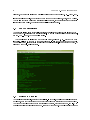
1.4 Explore the results
The results are stored in les, gathered by spatial unit. In each les, the values for variables are stored
as columns, each row corresponng to a data exchange time step (represented as a date and time).
The format of the les depends on the conguration of outputs, set through the run.xml le. The
default output directory is a directory named .openfluid/OPENFLUID.OUT and located into the user
1.5. BUDDIES
9
home directory (the user home directory may vary, depending on the used operating system). If you
prefer to store your outputs into another directory, you can specify it using command line options
passed to the engine (-o or --output-dir).
In order to process the results of your simulations, we encourage you to use software environments
such as R, Scilab or Octave, spreadsheets such as OpenOce Calc, GIS such as GRASS or QGIS.
1.5 Buddies
Buddies are small tools that help scientic developers in order to complete the modelling and/or
development works. They are usable from the command line, using the --buddyhelp, --buddy and
--buddyopts options. Four buddies are available:
• func2doc
• newfunc
• newdata
• convert
Options are given to buddies through a comma-separated list of key=value arguments, using the
--buddyopts command line option.
General usage is:
openfluid-engine buddy buddyname buddyopts abuddyopt=avalue,anotherbuddyopt=anothervalue
1.5.1 func2doc
The func2doc buddy extracts scientic information from the source code of simulation functions. It
uses the function signature and LATEX-formatted text placed between the <func2doc> and </func2doc>
tags (usually into C++ comments). From these sources of information, it builds a LATEX document
which could be compiled into a PDF document and/or HTML pages.
The func2doc buddy can also use information from an optional sub-directory named doc, located
in the same directory as the input source le. The information in the doc subdirectory should be
linked to the information from the source code using LATEX \input command. The func2doc buddy
is available on UNIX only systems (Linux, MacOSX).
Required options:
path for cpp le to parse
path for generated les
inputcpp
outputdir
Other options:
html
pdf
tplfile
set to 1 in order to generate documentation as HTML les
set to 1 in order to generate documentation as PDF le
path to template le
Usage example:
openfluid-engine buddy func2doc buddyopts inputcpp=/path/to/cppfile.cpp, outputdir=/path/to/out
10
CHAPTER 1. USAGE INFORMATION
1.5.2 newfunc
The newfunc buddy generate a skeleton source code of a simulation function, using given options.
Required options:
cppclass
funcid
C++ class name of the function
ID of the function
Other options:
email(s) of the author(s) of the function
name(s) of the author(s) of the function
path for generated les
authoremail
authorname
outputdir
Usage example:
openfluid-engine buddy newfunc buddyopts funcid=domain.subdomain.process.method,
outputdir=/path/to/outputdir
1.5.3 newdata
The newdata buddy generate a skeleton dataset.
Required options:
outputdir
Output directory for generated dataset
Usage example:
openfluid-engine buddy newdata buddyopts outputdir=/path/to/outputdir
1.5.4 convert
The convert buddy converts a dataset from a specic version format to another one. Currently,
conversion is possible from 1.3.x format to 1.4.x format, and from 1.4.x format to 1.5.x format
Required options:
convmode
inputdir
outputdir
Conversion mode. Available modes are: 13_14, 14_15
Input directory for dataset to convert
Output directory for converted dataset
Usage example:
openfluid-engine buddy convert buddyopts convmode=13_14, inputdir=/path/to/inputdir,outputdir=/
Chapter 2
FluidX le(s) format
This part of the manual describes the FluidX le(s) format. Refer to the "Usage" part of this manual
to run the simulation.
2.1 Overview
The FluidX le format is an XML based format for OpenFLUID input le(s). The OpenFLUID input
information can be provided by a one or many les using the FluidX format.
Whatever the input information is put into one or many les, the following sections must be dened
in the input le set:
•
The model section dened by the <model> tag
•
The spatial domain section dened by the <domain> tag
•
The run conguration section dened by the <run> tag
•
The outputs conguration section dened by the <output> tag
The order of the sections is not signicant. All of these sections must be inclosed into an openuid
section dened by the <openfluid> tag.
summary view of the XML tree for FluidX les
< openfluid >
< model >
<! -- here is the model definition -- >
</ model >
< domain >
<! -- here is the spatial domain definition , associated data and events -- >
</ domain >
< output >
<! -- here is the output configuration -- >
</ output >
< run >
<! -- here is the run configuration -- >
</ run >
</ openfluid >
11
12
CHAPTER 2. FLUIDX FILE(S) FORMAT
2.2 Sections
2.2.1 Model
The ux model is dened by an ordered set of data generators and simulations functions that will
be plugged to the OpenFLUID kernel. It denes the model for the simulation. It can also include
a global parameters section which applies to all simulation functions and generators. The global
parameters may be overridden by local parameters of simulation functions or generators.
The ux model must be dened in a section delimited by the <model> tag, and must be structured
following these rules:
•
Inside the <model> tag, there must be a set of <function>, <generator> and <gparams>
tags
•
Each <function> tag must bring a fileID attribute giving the identier of the simulation
function; the value of the fileID attribute must match the le name (without extension) of a
reachable and pluggable simulation function.
•
Each <function> tag may include zero to many <param> tags giving parameters to the function. Each <param> tag must bring a name attribute giving the name of the parameter and a
value attribute giving the value of the parameter. These parameters can be scalar or vector
of integer values, oating point values, string values. In case of vector, the values of the vector
are separated by a ; (semicolon).
•
Each <generator> tag must bring a varname attribute giving the name of the produced
variable, a unitclass attribute giving the unit class of the produced variable, a method attribute
giving the method used to produce the variable (fixed for constant value, random for random
value in a range, interp for a time-interpolated value from given data series, inject for an
injected value -no time interpolation- from given data series). An optional <varsize> attribute
can be set in order to produce a vector variable instead of a scalar variable.
•
Each <generator> tag may include zero to many <param> tags giving parameters to the
generator. Each <param> tag must bring a name attribute giving the name of the parameter
and a value attribute giving the value of the parameter.
•
A generator using the fixed method must provide a param named fixedvalue for the value
to produce.
•
A generator using the random method must provide a param named min and a param named
max delimiting the random range for the value to produce.
•
A generator using the interp method must provide a param named sources giving the data
sources lename and a param named distribution giving the distribution lename for the
value to produce (see appendix).
•
A generator using the inject method must provide a param named sources giving the data
sources lename and a param named distribution giving the distribution lename for the
value to produce (see appendix).
•
Each <gparams> tag may include zero to many <param> tags giving the global parameters.
Each <param> tag must bring a name attribute giving the name of the parameter and a value
attribute giving the value of the parameter.
example
<? xml version = " 1.0 " standalone = " yes " ? >
2.2. SECTIONS
13
< openfluid >
< model >
< gparams >
< param name = " gparam1 " value = " 100 " / >
< param name = " gparam2 " value = " 0.1 " / >
</ gparams >
< function fileID = " example . functionA " / >
< generator varname = " example . generator . fixed " unitclass = " EU1 " method = " fixed " varsize = " 11 " >
< param name = " fixedvalue " value = " 20 " / >
</ generator >
< generator varname = " example . generator . random " unitclass = " EU2 " method = " random " >
< param name = " min " value = " 20.53 " / >
< param name = " max " value = " 50 " / >
</ generator >
< function fileID = " example . functionB " >
< param name = " param1 " value = " strvalue " / >
< param name = " param2 " value = " 1.1 " / >
< param name = " gparam1 " value = " 50 " / >
</ function >
</ model >
</ openfluid >
Warning:
There must be only one model denition in the input dataset.
Warning:
The order of the simulation functions and data generators in the <model> section is
very important : the same order will be used for execution on the same time step
2.2.2 Spatial domain
Denition and relationships
The spatial domain is dened by a set of spatial units that are connected each others. These spatial
units are dened by a numerical identier (ID) and a class. They also include information about the
processing order of the unit in the class. Each unit can be connected to zero or many other units
from the same or a dierent unit class.
The spatial domain denition must be dened in a section delimited by the <definition> tag, which
is a sub-section of the domain tag, and must be structured following these rules:
•
Inside the <definition> tag, there must be a set of <unit> tags
•
Each <unit> tag must bring an ID attribute giving the identier of the unit, a class attribute
giving the class of the unit, a pcsorder attribute giving the process order in the class of the
unit
•
Each <unit> tag may include zero or many <to> tags giving the outgoing connections to other
units. Each <to> tag must bring an ID attribute giving the identier of the connected unit and
a class attribute giving the class of the connected unit
•
Each <unit> tag may include zero or many <childof> tags giving the parent units. Each
<childof> tag must bring an ID attribute giving the identier of the parent unit and a class
attribute giving the class of the parent unit
14
CHAPTER 2. FLUIDX FILE(S) FORMAT
example
<? xml version = " 1.0 " standalone = " yes " ? >
< openfluid >
< domain >
< definition >
< unit class = " PU " ID = " 1 " pcsorder = " 1 " / >
< unit class = " EU1 " ID = " 3 " pcsorder = " 1 " >
< to class = " EU1 " ID = " 11 " / >
< childof class = " PU " ID = " 1 " / >
</ unit >
< unit class = " EU1 " ID = " 11 " pcsorder = " 3 " >
< to class = " EU2 " ID = " 2 " / >
</ unit >
< unit class = " EU2 " ID = " 2 " pcsorder = " 1 " / >
</ definition >
</ domain >
</ openfluid >
Input data
The spatial domain input data are static data brought by units, usually properties and initial conditions
for each unit.
The spatial domain input data must be dened in a section delimited by the <inputdata> tag, which
is a sub-section of the domain tag, and must be structured following these rules:
•
The <inputdata> tag must bring a unitclass attribute giving the unit class to which input
data must be attached, and a colorder attribute giving the order of the contained columnformatted data
•
Inside the <inputdata> tag, there must be the input data as row-column text. As a rule, the
rst column is the ID of the unit in the class given through the the unitclass attribute of
<inputdata> tag, the following columns are values following the column order given through
the colorder attribute of the <inputdata> tag. Values for the data can be real, integer or
string.
example
<? xml version = " 1.0 " standalone = " yes " ? >
< openfluid >
< domain >
< inputdata unitclass = " EU1 " colorder = " indataA " >
3 1.1
11 7.5
</ inputdata >
< inputdata unitclass = " EU2 " colorder = " indataB1 ; indataB3 " >
2 18 STRVALX
</ inputdata >
</ domain >
</ openfluid >
15
2.2. SECTIONS
Note:
Old inputdata format, with <columns> and <data> tags are still useable. However, you
are encouraged to use the new FluidX le format.
Discrete events
The discrete events are events occuring on units, and that can be processed by simulation functions.
The spatial events must be dened in a section delimited by the <calendar> tag, which is a subsection of the domain tag, and must be structured following these rules:
•
Inside the <calendar> tag, there must be a set of <event> tags
•
Each <event> tag must bring a unitID and a unitclass attribute giving the unit on which
occurs the event, a date attribute giving the date and time of the event. The date format
must be "YYYY-MM-DD hh:mm:ss". The <event> tag may bring a name attribute and a a
category attribute, but they are actually ignored.
•
Each <event> tag may include zero to many <info> tags.
•
Each <info> tag give information about the event and must bring a key attribute giving the
name (the "key") of the info, and a value attribute giving the value for this key.
example
<? xml version = " 1.0 " standalone = " yes " ? >
< openfluid >
< domain >
< calendar >
< event unitclass = " EU1 " unitID = " 11 " date = " 1999 -12 -31 23 :59:59 " >
< info key = " when " value = " before " / >
< info key = " where " value = " 1 " / >
< info key = " var1 " value = " 1.13 " / >
< info key = " var2 " value = " EADGBE " / >
</ event >
< event unitclass = " EU2 " unitID = " 3 " date = " 2000 -02 -05 12 :37:51 " >
< info key = " var3 " value = " 152.27 " / >
< info key = " var4 " value = " XYZ " / >
</ event >
< event unitclass = " EU1 " unitID = " 11 " date = " 2000 -02 -25 12 :00:00 " >
< info key = " var1 " value = " 1.15 " / >
< info key = " var2 " value = " EADG " / >
</ event >
</ calendar >
</ domain >
</ openfluid >
2.2.3 Run conguration
The conguration of the simulation gives the simulation period, the data exchange time step, and
the optionnal progressive output parameters.
The run conguration must be dened in a section delimited by the <run> tag, and must be structured
following these rules:
•
Inside the <run> tag, there must be a <deltat> tag giving the data exchange time step (in
seconds)
16
CHAPTER 2. FLUIDX FILE(S) FORMAT
•
Inside the <run> tag, there must be a <period> tag giving the simulation period.
•
The <period> tag must bring a begin and an end attributes, giving the dates of the beginning and the end of the simulation period. The dates formats for these attributes must be
YYYY-MM-DD hh:mm:ss
•
Inside the <run> tag, there may be a <valuesbuffer> tag for the number of time steps kept
in memory. The number of step is given through a steps attribute. If not present, all values
are kept in memory.
•
Inside the <run> tag, there may be a <filesbuffer> tag for the size of the memory buer for
each le of results. The size is given in kilobytes through a kbytes attribute. If not present,
the default value is 2KB.
example
<? xml version = " 1.0 " standalone = " yes " ? >
< openfluid >
< run >
< deltat > 3600 </ deltat >
< period begin = " 2000 -01 -01 00 :00:00 " end = " 2000 -03 -27 01 :12:37 " / >
< valuesbuffer steps = " 10 " / >
< filesbuffer kbytes = " 8 " / >
</ run >
</ openfluid >
2.2.4 Outputs conguration
The conguration of the simulation outputs gives the description of the saved results.
The outputs conguration must be dened in a section delimited by the <output> tag, and must be
structured following these rules:
•
Inside the <output> tag, there must be one to many <files> tags, dening les formats for
saved data.
•
These <files> tags must bring a colsep attribute dening the separator strings between
columns, a dtformat attribute dening the date time format used (it could be 6cols, iso or
user dened using strftime() format whis is described in the appendix part of this document),
a commentchar attribute dening the string prexing lines of comments in output les. A
header attribute may be added giving the type of header in les. The values for this attribute
can be none for no header, info for a header giving commented information about the data
contained in the produced le(s), colnames-as-data for a rst line in le giving names of each
column, full for a complete header including both info and colnames-as-data headers (see
appendix for examples). If no header attribute is present, info header is used.
•
Inside the <files> tags, there must be one to many <set> tags. Each <set> tag will lead to
a set of les.
•
Each <set> tag must bring a name attribute dening the name of the set (this will be used as
a sux for generated output les), a unitsclass attribute and a unitsIDs attribute dening
the processed units, a vars attribute dening the processed variables. It may also bring an a
precision attribute giving the number of signicant digits for the values in the outputs les.
17
2.2. SECTIONS
The IDs for the unitsIDs attribute are semicolon-separated, the wildcard character ('*') can
be used to include all units IDs for the given class. The variables names for the vars attribute
are semicolon-separated, the wildcard character ('*') can be used to include all variables for
the given units class. The value for the precision attribute must be ≥ 0. If not provided, the
default value for the precision is 5.
example
<? xml version = " 1.0 " standalone = " yes " ? >
< openfluid >
< output >
< files colsep = " " dtformat = " % Y % m % d % H % M % S " commentchar = " % " >
< set name = " testRS " unitsclass = " RS " unitsIDs = " 51;232 " vars = " * " / >
< set name = " full " unitsclass = " SU " unitsIDs = " * " vars = " * " precision = " 7 " / >
</ files >
< files colsep = " " dtformat = " %Y -% m -% dT % H: % M: % S " commentchar = " # " header = " colnames - as - data " >
< set name = " full " unitsclass = " SU " unitsIDs = " * " vars = " * " precision = " 7 " / >
</ files >
</ output >
</ openfluid >
Chapter 3
Appendix
3.1 Command line options
-a, -auto-output-dir
-b, -buddy <arg>
-buddyhelp <arg>
generate automatic results output directory
run specied OpenFLUID buddy
display help message for specied OpenFLUID
buddy
-buddyopts <arg>
set options for specied OpenFLUID buddy
-c, -clean-output-dir
clean results output directory by removing existing
les
-f, -functions-list
list available functions (do not run the simulation)
-h, -help
display help message
-i, -input-dir <arg>
set dataset input directory
-k, -enable-simulation-profiling
enable time proling for functions
-o, -output-dir <arg>
set results output directory
-p, -functions-paths <arg>
add extra functions research paths
-q, -quiet
quiet display during simulation run
-r, -functions-report
print a report of available functions, with details
(do not run the simulation)
-s, -no-simreport
do not generate simulation report
-show-paths
print the used paths (do not run the simulation)
-u, -matching-functions-report <arg> print a report of functions matching the given
wildcard-based pattern (do not run the simulation)
-v, -verbose
verbose display during simulation
-version
get version (do not run the simulation)
-w, -project <arg>
set project directory
-x, -xml-functions-report
print a report of available functions in xml format,
with details (do not run the simulation)
-z, -no-result
do not write results les
3.2 Environment variables
The OpenFLUID framework takes into account the following environment variables (if they are set):
• OPENFLUID_FUNCS_PATH:
extra search paths for OpenFLUID simulation functions. The path
are separated by colon on UNIX systems, and by semicolon on Windows systems.
19
20
CHAPTER 3. APPENDIX
• OPENFLUID_INSTALL_PREFIX: overrides automatic detection of install path, useful on Windows
systems.
3.3 Structure of an OpenFLUID project
An OpenFLUID project can be run using OpenFLUID-Engine or OpenFLUID-Builder software. It is
a directory including:
•
a .openfluidprj le containing informations about the project,
•
an IN subdirectory containing the input dataset,
•
an OUT subdirectory as the default output directory, containing the simulation results if any.
The .openfluidprj contains the name of the project, the description of the project, the authors,
the creation date, the date of the latest modication, and a ag for incremental output directory
(this feature is currently disabled).
example of .openuidprj le
[ OpenFLUID Project ]
Name = a dummy project
Description =
Authors = John Doe
IncOutput = false
CreationDate =20110527 T121530
LastModDate =20110530 T151431
For example, if you wish to run a simulation with openfluid-engine, using the project located
in /absolute/path/to/workdir/a_dummy_project, the command line to use is:
openfluid-engine -w /absolute/path/to/workdir/a_dummy_project
3.4 Date-time formats used in outputs conguration
The output.xml le can use the ANSI strftime() standards formats for date time, through a format
string. The format string consists of zero or more conversion specications and ordinary characters.
A conversion specication consists of a % character and a terminating conversion character that
determines the conversion specication's behaviour. All ordinary characters (including the terminating
null byte) are copied unchanged into the array.
For example, the nineteenth of April, two-thousand seven, at eleven hours, ten minutes and
twenty-ve seconds formatted using dierent format strings:
•
"%d/%m/%Y %H:%M:%S" will give "19/04/2007 10:11:25"
•
"%Y-%m-%d %H.%M" will give "2007-04-19 10.11"
•
"%Y\t%m\t%d\t%H\t%M\t%S" will give "2007 04 19 10 11 25"
3.5. EXAMPLE OF AN INPUT DATASET AS A SINGLE FLUIDX FILE
21
List of available conversion specications:
Format
%a
%A
%b
%B
%c
%C
%d
%D
%e
%h
%H
%I
%j
%m
%M
%n
%p
%r
%R
%S
%t
%T
%u
%U
%V
%w
%W
%x
%X
%y
%Y
%Z
%%
Description
locale's abbreviated weekday name.
locale's full weekday name.
locale's abbreviated month name.
locale's full month name.
locale's appropriate date and time representation.
century number (the year divided by 100 and truncated to an integer) as a decimal
number [00-99].
day of the month as a decimal number [01,31].
same as %m/%d/%y.
day of the month as a decimal number [1,31]; a single digit is preceded by a space.
same as %b.
hour (24-hour clock) as a decimal number [00,23].
hour (12-hour clock) as a decimal number [01,12].
day of the year as a decimal number [001,366].
month as a decimal number [01,12].
minute as a decimal number [00,59].
is replaced by a newline character.
locale's equivalent of either a.m. or p.m.
time in a.m. and p.m. notation; in the POSIX locale this is equivalent to %I:%M:%S
%p.
time in 24 hour notation (%H:%M).
second as a decimal number [00,61].
is replaced by a tab character.
time (%H:%M:%S).
weekday as a decimal number [1,7], with 1 representing Monday.
week number of the year (Sunday as the rst day of the week) as a decimal number
[00,53].
week number of the year (Monday as the rst day of the week) as a decimal number
[01,53]. If the week containing 1 January has four or more days in the new year, then it
is considered week 1. Otherwise, it is the last week of the previous year, and the next
week is week 1.
weekday as a decimal number [0,6], with 0 representing Sunday.
week number of the year (Monday as the rst day of the week) as a decimal number
[00,53]. All days in a new year preceding the rst Monday are considered to be in week
0.
locale's appropriate date representation.
locale's appropriate time representation.
year without century as a decimal number [00,99].
year with century as a decimal number.
timezone name or abbreviation, or by no bytes if no timezone information exists.
character %.
3.5 Example of an input dataset as a single FluidX le
<? xml version = " 1.0 " standalone = " yes " ? >
< openfluid >
< model >
22
CHAPTER 3. APPENDIX
< gparams >
< param name = " gparam1 " value = " 100 " / >
< param name = " gparam2 " value = " 0.1 " / >
</ gparams >
< function fileID = " example . functionA " / >
< generator varname = " example . generator . fixed " unitclass = " EU1 "
method = " fixed " varsize = " 11 " >
< param name = " fixedvalue " value = " 20 " / >
</ generator >
< generator varname = " example . generator . random " unitclass = " EU2 "
method = " random " >
< param name = " min " value = " 20.53 " / >
< param name = " max " value = " 50 " / >
</ generator >
< function fileID = " example . functionB " >
< param name = " param1 " value = " strvalue " / >
< param name = " param2 " value = " 1.1 " / >
< param name = " gparam1 " value = " 50 " / >
</ function >
</ model >
< domain >
< definition >
< unit class = " PU " ID = " 1 " pcsorder = " 1 " / >
< unit class = " EU1 " ID = " 3 " pcsorder = " 1 " >
< to class = " EU1 " ID = " 11 " / >
< childof class = " PU " ID = " 1 " / >
</ unit >
< unit class = " EU1 " ID = " 11 " pcsorder = " 3 " >
< to class = " EU2 " ID = " 2 " / >
</ unit >
< unit class = " EU2 " ID = " 2 " pcsorder = " 1 " / >
</ definition >
< inputdata unitclass = " EU1 " colorder = " indataA " >
3 1.1
11 7.5
</ inputdata >
< inputdata unitclass = " EU2 " colorder = " indataB1 ; indataB3 " >
2 18 STRVALX
</ inputdata >
< calendar >
< event unitclass = " EU1 " unitID = " 11 " date = " 1999 -12 -31 23 :59:59 " >
< info key = " when " value = " before " / >
< info key = " where " value = " 1 " / >
< info key = " var1 " value = " 1.13 " / >
< info key = " var2 " value = " EADGBE " / >
</ event >
< event unitclass = " EU2 " unitID = " 3 " date = " 2000 -02 -05 12 :37:51 " >
< info key = " var3 " value = " 152.27 " / >
< info key = " var4 " value = " XYZ " / >
</ event >
< event unitclass = " EU1 " unitID = " 11 " date = " 2000 -02 -25 12 :00:00 " >
< info key = " var1 " value = " 1.15 " / >
< info key = " var2 " value = " EADG " / >
</ event >
</ calendar >
</ domain >
3.6. FILE FORMATS FOR INTERP OR INJECT DATA GENERATOR
23
< run >
< deltat > 3600 </ deltat >
< period begin = " 2000 -01 -01 00 :00:00 " end = " 2000 -03 -27 01 :12:37 " / >
< valuesbuffer steps = " 50 " / >
< filesbuffer kbytes = " 8 " / >
</ run >
< output >
< files colsep = " " dtformat = " % Y % m % d % H % M % S " commentchar = " % " >
< set name = " testRS " unitsclass = " RS " unitsIDs = " 51;232 " vars = " * " / >
< set name = " full " unitsclass = " SU " unitsIDs = " * " vars = " * " precision = " 7 " / >
</ files >
</ output >
</ openfluid >
3.6 File formats for interp or inject data generator
3.6.1 Sources
The sources le format is an XML based format which denes a list of sources les associated to an
unique ID.
The sources must be dened in a section delimited by the <datasources> tag, inside an <openfluid>
tag and must be structured following these rules:
•
Inside the <datasources> tag, there must be a set of <filesource> tags
•
Each <filesource> tag must bring an ID attribute giving the identier of source, and an file
attribute giving the name of the le containing the source of data. The les must be placed in
the input directory of the simulation.
example of a sources list le
<? xml version = " 1.0 " standalone = " yes " ? >
< openfluid >
< datasources >
< filesource ID = " 1 " file = " source1 . dat " / >
< filesource ID = " 2 " file = " source2 . dat " / >
</ datasources >
</ openfluid >
An associated source data le is a seven columns text le, containing a serie of values in time.
The six rst columns are the date using the following format YYYY MM DD HH MM SS. The 7th column
is the value itself.
example of a source data le
1999
1999
2000
2000
2000
12
12
01
01
01
31
31
01
01
01
12
23
00
00
01
00
00
30
40
30
00
00
00
00
00
-1.0
-5.0
-15.0
-5.0
-15.0
24
CHAPTER 3. APPENDIX
3.6.2 Distribution
A distribution le is a two column le associating a unit ID (1st column) to a source ID (2nd column).
example of distribution le
2
3
4
5
2
1
2
1
3.7 Header types examples
The following examples show output les for 2 variables (var1 and var2) extracted from a 6 hours
simulation ran at a time step of an hour.
3.7.1 none
example of an output data le
2000 -01 -01
2000 -01 -01
2000 -01 -01
2000 -01 -01
2000 -01 -01
2000 -01 -01
00:00:00;0.00000;1.00000
01:00:00;2.00000;3.00000
02:00:00;4.00000;5.00000
03:00:00;6.00000;7.00000
04:00:00;8.00000;9.00000
05:00:00;10.00000;11.00000
3.7.2 info
example of an output data le
%
%
%
%
%
simulation ID : 20110905 - VZIRXC
file : TestUnits2_full - info . scalars . out
date : 2011 - Sep -05 10:23:17.394061
unit : TestUnits #2
scalar variables order ( after date and time columns ): var1 var2
2000 -01 -01
2000 -01 -01
2000 -01 -01
2000 -01 -01
2000 -01 -01
2000 -01 -01
00:00:00;0.00000;1.00000
01:00:00;2.00000;3.00000
02:00:00;4.00000;5.00000
03:00:00;6.00000;7.00000
04:00:00;8.00000;9.00000
05:00:00;10.00000;11.00000
3.7.3 colnames-as-data
example of an output data le
datetime ; var1 ; var2
2000 -01 -01 00:00:00;0.00000;1.00000
2000 -01 -01 01:00:00;2.00000;3.00000
2000 -01 -01 02:00:00;4.00000;5.00000
2000 -01 -01 03:00:00;6.00000;7.00000
2000 -01 -01 04:00:00;8.00000;9.00000
2000 -01 -01 05:00:00;10.00000;11.00000
25
3.8. USEFUL LINKS
3.7.4 full
example of an output data le
%
%
%
%
%
simulation ID : 20110905 - VZIRXC
file : TestUnits2_full - info . scalars . out
date : 2011 - Sep -05 10:23:17.394061
unit : TestUnits #2
scalar variables order ( after date and time columns ): var1 var2
datetime ; var1 ; var2
2000 -01 -01 00:00:00;0.00000;1.00000
2000 -01 -01 01:00:00;2.00000;3.00000
2000 -01 -01 02:00:00;4.00000;5.00000
2000 -01 -01 03:00:00;6.00000;7.00000
2000 -01 -01 04:00:00;8.00000;9.00000
2000 -01 -01 05:00:00;10.00000;11.00000
3.8 Useful links
3.8.1 OpenFLUID project
•
OpenFLUID web site : http://www.umr-lisah.fr/openuid/
•
OpenFLUID web community : http://www.umr-lisah.fr/openuid/community/
•
OpenFLUID on SourceSup (software forge): https://sourcesup.cru.fr/projects/openuid/
3.8.2 External tools
•
Geany : http://www.geany.org/
•
Gnuplot : http://www.gnuplot.info/
•
GRASS GIS : http://grass.itc.it/
•
jEdit : http://www.jedit.org/
•
Octave : http://www.gnu.org/software/octave/
•
QGIS : http://www.qgis.org/
•
R : http://www.r-project.org/
•
Scilab : http://www.scilab.org/
•
VisIt : visit.llnl.gov