1
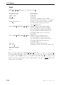
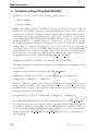
FLUENT 6.3
September 2006
UDF Manual
c 2006 by Fluent Inc.
Copyright All Rights Reserved. No part of this document may be reproduced or otherwise used in
any form without express written permission from Fluent Inc.
Airpak, FIDAP, FLUENT, FLUENT for CATIA V5, FloWizard, GAMBIT, Icemax, Icepak,
Icepro, Icewave, Icechip, MixSim, and POLYFLOW are registered trademarks of Fluent
Inc. All other products or name brands are trademarks of their respective holders.
CHEMKIN is a registered trademark of Reaction Design Inc.
Portions of this program include material copyrighted by PathScale Corporation
2003-2004.
Fluent Inc.
Centerra Resource Park
10 Cavendish Court
Lebanon, NH 03766
Contents
Preface
i
1 Overview
1-1
1.1
What is a User-Defined Function (UDF)? . . . . . . . . . . . . . . . . .
1-1
1.2
Why Use UDFs? . . . . . . . . . . . . . . . . . . . . . . . . . . . . . . .
1-3
1.3
Limitations . . . . . . . . . . . . . . . . . . . . . . . . . . . . . . . . . .
1-3
1.4
Defining Your UDF Using DEFINE Macros . . . . . . . . . . . . . . . . .
1-3
1.4.1
Including the udf.h Header File in Your Source File . . . . . . .
1-5
Interpreting and Compiling UDFs . . . . . . . . . . . . . . . . . . . . . .
1-6
1.5.1
Differences Between Interpreted and Compiled UDFs . . . . . . .
1-7
1.6
Hooking UDFs to Your FLUENT Model . . . . . . . . . . . . . . . . . .
1-8
1.7
Grid Terminology . . . . . . . . . . . . . . . . . . . . . . . . . . . . . . .
1-8
1.8
Data Types in FLUENT . . . . . . . . . . . . . . . . . . . . . . . . . . . 1-10
1.9
UDF Calling Sequence in the Solution Process . . . . . . . . . . . . . . . 1-12
1.5
1.10 Special Considerations for Multiphase UDFs . . . . . . . . . . . . . . . . 1-17
1.10.1
Multiphase-specific Data Types . . . . . . . . . . . . . . . . . . . 1-17
2 DEFINE Macros
2-1
2.1
Introduction
. . . . . . . . . . . . . . . . . . . . . . . . . . . . . . . . .
2-1
2.2
General Purpose DEFINE Macros . . . . . . . . . . . . . . . . . . . . . .
2-2
2.2.1
DEFINE ADJUST . . . . . . . . . . . . . . . . . . . . . . . . . . . .
2-4
2.2.2
DEFINE DELTAT . . . . . . . . . . . . . . . . . . . . . . . . . . . .
2-7
2.2.3
DEFINE EXECUTE AT END . . . . . . . . . . . . . . . . . . . . . . .
2-9
2.2.4
DEFINE EXECUTE AT EXIT . . . . . . . . . . . . . . . . . . . . . . 2-11
2.2.5
DEFINE EXECUTE FROM GUI . . . . . . . . . . . . . . . . . . . . . 2-12
c Fluent Inc. September 11, 2006
i
CONTENTS
2.3
ii
2.2.6
DEFINE EXECUTE ON LOADING . . . . . . . . . . . . . . . . . . . . 2-14
2.2.7
DEFINE INIT . . . . . . . . . . . . . . . . . . . . . . . . . . . . . 2-17
2.2.8
DEFINE ON DEMAND . . . . . . . . . . . . . . . . . . . . . . . . . . 2-19
2.2.9
DEFINE RW FILE . . . . . . . . . . . . . . . . . . . . . . . . . . . 2-22
Model-Specific DEFINE Macros . . . . . . . . . . . . . . . . . . . . . . . . 2-24
2.3.1
DEFINE CHEM STEP . . . . . . . . . . . . . . . . . . . . . . . . . . 2-29
2.3.2
DEFINE CPHI . . . . . . . . . . . . . . . . . . . . . . . . . . . . . 2-31
2.3.3
DEFINE DIFFUSIVITY . . . . . . . . . . . . . . . . . . . . . . . . 2-32
2.3.4
DEFINE DOM DIFFUSE REFLECTIVITY . . . . . . . . . . . . . . . . 2-34
2.3.5
DEFINE DOM SOURCE . . . . . . . . . . . . . . . . . . . . . . . . . 2-36
2.3.6
DEFINE DOM SPECULAR REFLECTIVITY . . . . . . . . . . . . . . . 2-38
2.3.7
DEFINE GRAY BAND ABS COEFF . . . . . . . . . . . . . . . . . . . . 2-40
2.3.8
DEFINE HEAT FLUX . . . . . . . . . . . . . . . . . . . . . . . . . . 2-42
2.3.9
DEFINE NET REACTION RATE . . . . . . . . . . . . . . . . . . . . . 2-44
2.3.10
DEFINE NOX RATE
2.3.11
DEFINE PR RATE . . . . . . . . . . . . . . . . . . . . . . . . . . . 2-50
2.3.12
DEFINE PRANDTL UDFs . . . . . . . . . . . . . . . . . . . . . . . 2-55
2.3.13
DEFINE PROFILE . . . . . . . . . . . . . . . . . . . . . . . . . . . 2-63
2.3.14
DEFINE PROPERTY UDFs . . . . . . . . . . . . . . . . . . . . . . . 2-76
2.3.15
DEFINE SCAT PHASE FUNC . . . . . . . . . . . . . . . . . . . . . . 2-84
2.3.16
DEFINE SOLAR INTENSITY . . . . . . . . . . . . . . . . . . . . . . 2-87
2.3.17
DEFINE SOURCE . . . . . . . . . . . . . . . . . . . . . . . . . . . . 2-89
2.3.18
DEFINE SOX RATE
2.3.19
DEFINE SR RATE . . . . . . . . . . . . . . . . . . . . . . . . . . . 2-97
2.3.20
DEFINE TURB PREMIX SOURCE . . . . . . . . . . . . . . . . . . . . 2-101
2.3.21
DEFINE TURBULENT VISCOSITY . . . . . . . . . . . . . . . . . . . 2-103
2.3.22
DEFINE VR RATE . . . . . . . . . . . . . . . . . . . . . . . . . . . 2-107
2.3.23
DEFINE WALL FUNCTIONS
. . . . . . . . . . . . . . . . . . . . . . . . . . 2-46
. . . . . . . . . . . . . . . . . . . . . . . . . . 2-92
. . . . . . . . . . . . . . . . . . . . . . 2-111
c Fluent Inc. September 11, 2006
CONTENTS
2.4
2.5
2.6
Multiphase DEFINE Macros . . . . . . . . . . . . . . . . . . . . . . . . . 2-113
2.4.1
DEFINE CAVITATION RATE . . . . . . . . . . . . . . . . . . . . . . 2-115
2.4.2
DEFINE EXCHANGE PROPERTY
2.4.3
DEFINE HET RXN RATE . . . . . . . . . . . . . . . . . . . . . . . . 2-123
2.4.4
DEFINE MASS TRANSFER . . . . . . . . . . . . . . . . . . . . . . . 2-129
2.4.5
DEFINE VECTOR EXCHANGE PROPERTY . . . . . . . . . . . . . . . . 2-132
. . . . . . . . . . . . . . . . . . . . 2-118
Discrete Phase Model (DPM) DEFINE Macros . . . . . . . . . . . . . . . 2-135
2.5.1
DEFINE DPM BC . . . . . . . . . . . . . . . . . . . . . . . . . . . . 2-137
2.5.2
DEFINE DPM BODY FORCE . . . . . . . . . . . . . . . . . . . . . . . 2-145
2.5.3
DEFINE DPM DRAG
2.5.4
DEFINE DPM EROSION
2.5.5
DEFINE DPM HEAT MASS . . . . . . . . . . . . . . . . . . . . . . . 2-155
2.5.6
DEFINE DPM INJECTION INIT . . . . . . . . . . . . . . . . . . . . 2-158
2.5.7
DEFINE DPM LAW . . . . . . . . . . . . . . . . . . . . . . . . . . . 2-162
2.5.8
DEFINE DPM OUTPUT . . . . . . . . . . . . . . . . . . . . . . . . . 2-164
2.5.9
DEFINE DPM PROPERTY . . . . . . . . . . . . . . . . . . . . . . . . 2-168
2.5.10
DEFINE DPM SCALAR UPDATE . . . . . . . . . . . . . . . . . . . . . 2-172
2.5.11
DEFINE DPM SOURCE . . . . . . . . . . . . . . . . . . . . . . . . . 2-176
2.5.12
DEFINE DPM SPRAY COLLIDE . . . . . . . . . . . . . . . . . . . . . 2-178
2.5.13
DEFINE DPM SWITCH . . . . . . . . . . . . . . . . . . . . . . . . . 2-181
2.5.14
DEFINE DPM TIMESTEP . . . . . . . . . . . . . . . . . . . . . . . . 2-186
2.5.15
DEFINE DPM VP EQUILIB . . . . . . . . . . . . . . . . . . . . . . . 2-189
. . . . . . . . . . . . . . . . . . . . . . . . . . 2-147
. . . . . . . . . . . . . . . . . . . . . . . . 2-149
Dynamic Mesh DEFINE Macros . . . . . . . . . . . . . . . . . . . . . . . 2-192
2.6.1
DEFINE CG MOTION . . . . . . . . . . . . . . . . . . . . . . . . . . 2-193
2.6.2
DEFINE GEOM . . . . . . . . . . . . . . . . . . . . . . . . . . . . . 2-196
2.6.3
DEFINE GRID MOTION
2.6.4
DEFINE SDOF PROPERTIES . . . . . . . . . . . . . . . . . . . . . . 2-201
c Fluent Inc. September 11, 2006
. . . . . . . . . . . . . . . . . . . . . . . . 2-198
iii
CONTENTS
2.7
User-Defined Scalar (UDS) Transport Equation DEFINE Macros . . . . . 2-205
2.7.1
Introduction . . . . . . . . . . . . . . . . . . . . . . . . . . . . . 2-205
2.7.2
DEFINE ANISOTROPIC DIFFUSIVITY
2.7.3
DEFINE UDS FLUX
2.7.4
DEFINE UDS UNSTEADY . . . . . . . . . . . . . . . . . . . . . . . . 2-215
. . . . . . . . . . . . . . . . 2-207
. . . . . . . . . . . . . . . . . . . . . . . . . . 2-211
3 Additional Macros for Writing UDFs
3.1
Introduction
. . . . . . . . . . . . . . . . . . . . . . . . . . . . . . . . .
3-2
3.2
Data Access Macros . . . . . . . . . . . . . . . . . . . . . . . . . . . . .
3-5
3.2.1
Introduction . . . . . . . . . . . . . . . . . . . . . . . . . . . . .
3-5
3.2.2
Node Macros . . . . . . . . . . . . . . . . . . . . . . . . . . . . .
3-6
3.2.3
Cell Macros . . . . . . . . . . . . . . . . . . . . . . . . . . . . . .
3-7
3.2.4
Face Macros . . . . . . . . . . . . . . . . . . . . . . . . . . . . . 3-19
3.2.5
Connectivity Macros . . . . . . . . . . . . . . . . . . . . . . . . . 3-22
3.2.6
Special Macros . . . . . . . . . . . . . . . . . . . . . . . . . . . . 3-26
3.2.7
Model-Specific Macros . . . . . . . . . . . . . . . . . . . . . . . . 3-32
3.2.8
User-Defined Scalar (UDS) Transport Equation Macros . . . . . 3-39
3.2.9
User-Defined Memory (UDM) Macros . . . . . . . . . . . . . . . 3-42
3.3
3.4
3.5
iv
3-1
Looping Macros . . . . . . . . . . . . . . . . . . . . . . . . . . . . . . . . 3-51
3.3.1
Multiphase Looping Macros . . . . . . . . . . . . . . . . . . . . . 3-55
3.3.2
Advanced Multiphase Macros . . . . . . . . . . . . . . . . . . . . 3-59
Vector and Dimension Macros . . . . . . . . . . . . . . . . . . . . . . . . 3-64
3.4.1
Macros for Dealing with Two and Three Dimensions . . . . . . . 3-64
3.4.2
The ND Macros . . . . . . . . . . . . . . . . . . . . . . . . . . . . 3-64
3.4.3
The NV Macros . . . . . . . . . . . . . . . . . . . . . . . . . . . . 3-66
3.4.4
Vector Operation Macros . . . . . . . . . . . . . . . . . . . . . . 3-67
Time-Dependent Macros . . . . . . . . . . . . . . . . . . . . . . . . . . . 3-69
c Fluent Inc. September 11, 2006
CONTENTS
3.6
Scheme Macros . . . . . . . . . . . . . . . . . . . . . . . . . . . . . . . . 3-71
3.6.1
Defining a Scheme Variable in the Text Interface . . . . . . . . . 3-71
3.6.2
Accessing a Scheme Variable in the Text Interface . . . . . . . . 3-72
3.6.3
Changing a Scheme Variable to Another Value in the Text Interface 3-72
3.6.4
Accessing a Scheme Variable in a UDF . . . . . . . . . . . . . . 3-72
3.7
Input/Output Macros . . . . . . . . . . . . . . . . . . . . . . . . . . . . 3-73
3.8
Miscellaneous Macros . . . . . . . . . . . . . . . . . . . . . . . . . . . . 3-74
4 Interpreting UDFs
4.1
Introduction
4-1
. . . . . . . . . . . . . . . . . . . . . . . . . . . . . . . . .
4-1
4.1.1
Location of the udf.h File . . . . . . . . . . . . . . . . . . . . .
4-2
4.1.2
Limitations . . . . . . . . . . . . . . . . . . . . . . . . . . . . . .
4-2
4.2
Interpreting a UDF Source File Using the Interpreted UDFs Panel . . . .
4-3
4.3
Common Errors Made While Interpreting A Source File . . . . . . . . .
4-5
4.4
Special Considerations for Parallel FLUENT . . . . . . . . . . . . . . . .
4-7
5 Compiling UDFs
5.1
. . . . . . . . . . . . . . . . . . . . . . . . . . . . . . . . .
5-2
5.1.1
Location of the udf.h File . . . . . . . . . . . . . . . . . . . . .
5-3
5.1.2
Compilers . . . . . . . . . . . . . . . . . . . . . . . . . . . . . . .
5-4
5.2
Compile a UDF Using the GUI . . . . . . . . . . . . . . . . . . . . . . .
5-4
5.3
Compile a UDF Using the TUI . . . . . . . . . . . . . . . . . . . . . . . 5-11
5.4
Introduction
5-1
5.3.1
Set Up the Directory Structure . . . . . . . . . . . . . . . . . . . 5-11
5.3.2
Build the UDF Library . . . . . . . . . . . . . . . . . . . . . . . 5-14
5.3.3
Load the UDF Library . . . . . . . . . . . . . . . . . . . . . . . 5-19
Link Precompiled Object Files From Non-FLUENT Sources . . . . . . . . 5-19
5.4.1
Example - Link Precompiled Objects to FLUENT . . . . . . . . . 5-19
5.5
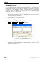
Load and Unload Libraries Using the UDF Library Manager Panel . . . . 5-25
5.6
Common Errors When Building and Loading a UDF Library . . . . . . . 5-27
5.7
Special Considerations for Parallel FLUENT . . . . . . . . . . . . . . . . 5-28
c Fluent Inc. September 11, 2006
v
CONTENTS
6 Hooking UDFs to FLUENT
6.1
6.2
vi
Hooking General Purpose UDFs
6-1
. . . . . . . . . . . . . . . . . . . . . .
6-1
6.1.1
Hooking DEFINE ADJUST UDFs . . . . . . . . . . . . . . . . . . .
6-2
6.1.2
Hooking DEFINE DELTAT UDFs . . . . . . . . . . . . . . . . . . .
6-4
6.1.3
Hooking DEFINE EXECUTE AT END UDFs . . . . . . . . . . . . . .
6-6
6.1.4
Hooking DEFINE EXECUTE AT EXIT UDFs . . . . . . . . . . . . .
6-8
6.1.5
Hooking DEFINE INIT UDFs . . . . . . . . . . . . . . . . . . . . 6-10
6.1.6
Hooking DEFINE ON DEMAND UDFs . . . . . . . . . . . . . . . . . 6-12
6.1.7
Hooking DEFINE RW FILE UDFs . . . . . . . . . . . . . . . . . . 6-13
6.1.8
User-Defined Memory Storage . . . . . . . . . . . . . . . . . . . 6-15
Hooking Model-Specific UDFs . . . . . . . . . . . . . . . . . . . . . . . . 6-15
6.2.1
Hooking DEFINE CHEM STEP UDFs . . . . . . . . . . . . . . . . . 6-16
6.2.2
Hooking DEFINE CPHI UDFs . . . . . . . . . . . . . . . . . . . . 6-17
6.2.3
Hooking DEFINE DIFFUSIVITY UDFs . . . . . . . . . . . . . . . . 6-18
6.2.4
Hooking DEFINE DOM DIFFUSE REFLECTIVITY UDFs . . . . . . . 6-20
6.2.5
Hooking DEFINE DOM SOURCE UDFs . . . . . . . . . . . . . . . . 6-21
6.2.6
Hooking DEFINE DOM SPECULAR REFLECTIVITY UDFs . . . . . . . 6-22
6.2.7
Hooking DEFINE GRAY BAND ABS COEFF UDFs . . . . . . . . . . . 6-23
6.2.8
Hooking DEFINE HEAT FLUX UDFs . . . . . . . . . . . . . . . . . 6-24
6.2.9
Hooking DEFINE NET REACTION RATE UDFs . . . . . . . . . . . . 6-25
6.2.10
Hooking DEFINE NOX RATE UDFs . . . . . . . . . . . . . . . . . . 6-27
6.2.11
Hooking DEFINE PR RATE UDFs . . . . . . . . . . . . . . . . . . 6-29
6.2.12
Hooking DEFINE PRANDTL UDFs . . . . . . . . . . . . . . . . . . 6-30
6.2.13
Hooking DEFINE PROFILE UDFs . . . . . . . . . . . . . . . . . . 6-31
6.2.14
Hooking DEFINE PROPERTY UDFs . . . . . . . . . . . . . . . . . . 6-36
6.2.15
Hooking DEFINE SCAT PHASE FUNC UDFs . . . . . . . . . . . . . 6-38
6.2.16
Hooking DEFINE SOLAR INTENSITY UDFs . . . . . . . . . . . . . 6-40
6.2.17
Hooking DEFINE SOURCE UDFs . . . . . . . . . . . . . . . . . . . 6-42
6.2.18
Hooking DEFINE SOX RATE UDFs . . . . . . . . . . . . . . . . . . 6-44
c Fluent Inc. September 11, 2006
CONTENTS
6.3
6.4
6.2.19
Hooking DEFINE SR RATE UDFs . . . . . . . . . . . . . . . . . . 6-46
6.2.20
Hooking DEFINE TURB PREMIX SOURCE UDFs . . . . . . . . . . . 6-47
6.2.21
Hooking DEFINE TURBULENT VISCOSITY UDFs . . . . . . . . . . 6-48
6.2.22
Hooking DEFINE VR RATE UDFs . . . . . . . . . . . . . . . . . . 6-49
6.2.23
Hooking DEFINE WALL FUNCTIONS UDFs . . . . . . . . . . . . . . 6-50
Hooking Multiphase UDFs . . . . . . . . . . . . . . . . . . . . . . . . . . 6-51
6.3.1
Hooking DEFINE CAVITATION RATE UDFs . . . . . . . . . . . . . 6-51
6.3.2
Hooking DEFINE EXCHANGE PROPERTY UDFs . . . . . . . . . . . . 6-53
6.3.3
Hooking DEFINE HET RXN RATE UDFs . . . . . . . . . . . . . . . 6-55
6.3.4
Hooking DEFINE MASS TRANSFER UDFs . . . . . . . . . . . . . . 6-56
6.3.5
Hooking DEFINE VECTOR EXCHANGE PROPERTY UDFs . . . . . . . 6-57
Hooking Discrete Phase Model (DPM) UDFs . . . . . . . . . . . . . . . 6-59
6.4.1
Hooking DEFINE DPM BC UDFs . . . . . . . . . . . . . . . . . . . 6-59
6.4.2
Hooking DEFINE DPM BODY FORCE UDFs . . . . . . . . . . . . . . 6-61
6.4.3
Hooking DEFINE DPM DRAG UDFs . . . . . . . . . . . . . . . . . . 6-62
6.4.4
Hooking DEFINE DPM EROSION UDFs . . . . . . . . . . . . . . . . 6-63
6.4.5
Hooking DEFINE DPM HEAT MASS UDFs . . . . . . . . . . . . . . . 6-64
6.4.6
Hooking DEFINE DPM INJECTION INIT UDFs . . . . . . . . . . . 6-66
6.4.7
Hooking DEFINE DPM LAW UDFs . . . . . . . . . . . . . . . . . . 6-68
6.4.8
Hooking DEFINE DPM OUTPUT UDFs . . . . . . . . . . . . . . . . 6-69
6.4.9
Hooking DEFINE DPM PROPERTY UDFs . . . . . . . . . . . . . . . 6-70
6.4.10
Hooking DEFINE DPM SCALAR UPDATE UDFs . . . . . . . . . . . . 6-72
6.4.11
Hooking DEFINE DPM SOURCE UDFs . . . . . . . . . . . . . . . . 6-73
6.4.12
Hooking DEFINE DPM SPRAY COLLIDE UDFs . . . . . . . . . . . . 6-74
6.4.13
Hooking DEFINE DPM SWITCH UDFs . . . . . . . . . . . . . . . . 6-76
6.4.14
Hooking DEFINE DPM TIMESTEP UDFs . . . . . . . . . . . . . . . 6-77
6.4.15
Hooking DEFINE DPM VP EQUILIB UDFs . . . . . . . . . . . . . . 6-78
c Fluent Inc. September 11, 2006
vii
CONTENTS
6.5
6.6
6.7
Hooking Dynamic Mesh UDFs . . . . . . . . . . . . . . . . . . . . . . . 6-79
6.5.1
Hooking DEFINE CG MOTION UDFs . . . . . . . . . . . . . . . . . 6-79
6.5.2
Hooking DEFINE GEOM UDFs . . . . . . . . . . . . . . . . . . . . 6-81
6.5.3
Hooking DEFINE GRID MOTION UDFs . . . . . . . . . . . . . . . . 6-83
6.5.4
Hooking DEFINE SDOF PROPERTIES UDFs . . . . . . . . . . . . . 6-85
Hooking User-Defined Scalar (UDS) Transport Equation UDFs . . . . . 6-87
6.6.1
Hooking DEFINE ANISOTROPIC DIFFUSIVITY UDFs . . . . . . . . 6-87
6.6.2
Hooking DEFINE UDS FLUX UDFs . . . . . . . . . . . . . . . . . . 6-90
6.6.3
Hooking DEFINE UDS UNSTEADY UDFs . . . . . . . . . . . . . . . 6-91
Common Errors While Hooking a UDF to FLUENT . . . . . . . . . . . . 6-92
7 Parallel Considerations
7.1
viii
7-1
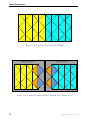
Overview of Parallel FLUENT . . . . . . . . . . . . . . . . . . . . . . . .
7-1
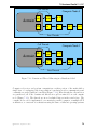
7.1.1
Command Transfer and Communication . . . . . . . . . . . . . .
7-4
7.2
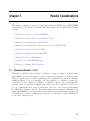
Cells and Faces in a Partitioned Grid . . . . . . . . . . . . . . . . . . . .
7-7
7.3
Parallelizing Your Serial UDF . . . . . . . . . . . . . . . . . . . . . . . . 7-11
7.4
Parallelization of Discrete Phase Model (DPM) UDFs
7.5
Macros for Parallel UDFs . . . . . . . . . . . . . . . . . . . . . . . . . . 7-13
. . . . . . . . . . 7-12
7.5.1
Compiler Directives . . . . . . . . . . . . . . . . . . . . . . . . . 7-13
7.5.2
Communicating Between the Host and Node Processes . . . . . . 7-16
7.5.3
Predicates . . . . . . . . . . . . . . . . . . . . . . . . . . . . . . 7-18
7.5.4
Global Reduction Macros . . . . . . . . . . . . . . . . . . . . . . 7-19
7.5.5
Looping Macros . . . . . . . . . . . . . . . . . . . . . . . . . . . 7-23
7.5.6
Cell and Face Partition ID Macros . . . . . . . . . . . . . . . . . 7-30
7.5.7
Message Displaying Macros . . . . . . . . . . . . . . . . . . . . . 7-31
7.5.8
Message Passing Macros . . . . . . . . . . . . . . . . . . . . . . . 7-32
7.5.9
Macros for Exchanging Data Between Compute Nodes . . . . . . 7-36
7.6
Limitations of Parallel UDFs . . . . . . . . . . . . . . . . . . . . . . . . 7-37
7.7
Process Identification . . . . . . . . . . . . . . . . . . . . . . . . . . . . . 7-39
c Fluent Inc. September 11, 2006
CONTENTS
7.8
Parallel UDF Example . . . . . . . . . . . . . . . . . . . . . . . . . . . . 7-41
7.9
Writing Files in Parallel . . . . . . . . . . . . . . . . . . . . . . . . . . . 7-44
8 Examples
8.1
8.2
8-1
Step-By-Step UDF Example . . . . . . . . . . . . . . . . . . . . . . . . .
8-1
8.1.1
Process Overview . . . . . . . . . . . . . . . . . . . . . . . . . .
8-1
8.1.2
Step 1: Define Your Problem . . . . . . . . . . . . . . . . . . . .
8-3
8.1.3
Step 2: Create a C Source File . . . . . . . . . . . . . . . . . . .
8-5
8.1.4
Step 3: Start FLUENT and Read (or Set Up) the Case File . . .
8-6
8.1.5
Step 4: Interpret or Compile the Source File . . . . . . . . . . .
8-6
8.1.6
Step 5: Hook the UDF to FLUENT . . . . . . . . . . . . . . . . . 8-13
8.1.7
Step 6: Run the Calculation . . . . . . . . . . . . . . . . . . . . 8-14
8.1.8
Step 7: Analyze the Numerical Solution and Compare
to Expected Results . . . . . . . . . . . . . . . . . . . . . . . . . 8-14
Detailed UDF Examples . . . . . . . . . . . . . . . . . . . . . . . . . . . 8-15
8.2.1
Boundary Conditions . . . . . . . . . . . . . . . . . . . . . . . . 8-15
8.2.2
Source Terms . . . . . . . . . . . . . . . . . . . . . . . . . . . . . 8-26
8.2.3
Physical Properties . . . . . . . . . . . . . . . . . . . . . . . . . 8-33
8.2.4
Reaction Rates . . . . . . . . . . . . . . . . . . . . . . . . . . . . 8-38
8.2.5
User-Defined Scalars . . . . . . . . . . . . . . . . . . . . . . . . . 8-44
A C Programming Basics
A.1 Introduction
A-1
. . . . . . . . . . . . . . . . . . . . . . . . . . . . . . . . . A-1
A.2 Commenting Your C Code . . . . . . . . . . . . . . . . . . . . . . . . . . A-2
A.3 C Data Types in FLUENT . . . . . . . . . . . . . . . . . . . . . . . . . . A-2
A.4 Constants . . . . . . . . . . . . . . . . . . . . . . . . . . . . . . . . . . . A-3
A.5 Variables . . . . . . . . . . . . . . . . . . . . . . . . . . . . . . . . . . . A-3
A.5.1
Declaring Variables . . . . . . . . . . . . . . . . . . . . . . . . . A-4
A.5.2
External Variables . . . . . . . . . . . . . . . . . . . . . . . . . . A-5
A.5.3
Static Variables . . . . . . . . . . . . . . . . . . . . . . . . . . . A-7
c Fluent Inc. September 11, 2006
ix
CONTENTS
A.6 User-Defined Data Types . . . . . . . . . . . . . . . . . . . . . . . . . . A-8
A.7 Casting . . . . . . . . . . . . . . . . . . . . . . . . . . . . . . . . . . . . A-8
A.8 Functions . . . . . . . . . . . . . . . . . . . . . . . . . . . . . . . . . . . A-8
A.9 Arrays . . . . . . . . . . . . . . . . . . . . . . . . . . . . . . . . . . . . . A-9
A.10 Pointers . . . . . . . . . . . . . . . . . . . . . . . . . . . . . . . . . . . . A-9
A.11 Control Statements . . . . . . . . . . . . . . . . . . . . . . . . . . . . . . A-11
A.11.1 if Statement . . . . . . . . . . . . . . . . . . . . . . . . . . . . . A-11
A.11.2 if-else Statement . . . . . . . . . . . . . . . . . . . . . . . . . A-11
A.11.3 for Loops . . . . . . . . . . . . . . . . . . . . . . . . . . . . . . A-12
A.12 Common C Operators . . . . . . . . . . . . . . . . . . . . . . . . . . . . A-13
A.12.1 Arithmetic Operators . . . . . . . . . . . . . . . . . . . . . . . . A-13
A.12.2 Logical Operators . . . . . . . . . . . . . . . . . . . . . . . . . . A-13
A.13 C Library Functions . . . . . . . . . . . . . . . . . . . . . . . . . . . . . A-14
A.13.1 Trigonometric Functions . . . . . . . . . . . . . . . . . . . . . . . A-14
A.13.2 Miscellaneous Mathematical Functions . . . . . . . . . . . . . . . A-14
A.13.3 Standard I/O Functions . . . . . . . . . . . . . . . . . . . . . . . A-15
A.14 Preprocessor Directives
. . . . . . . . . . . . . . . . . . . . . . . . . . . A-18
A.15 Comparison with FORTRAN . . . . . . . . . . . . . . . . . . . . . . . . A-19
B DEFINE Macro Definitions
B.1 General Solver DEFINE Macros
B-1
. . . . . . . . . . . . . . . . . . . . . . . B-1
B.2 Model-Specific DEFINE Macro Definitions . . . . . . . . . . . . . . . . . . B-2
B.3 Multiphase DEFINE Macros . . . . . . . . . . . . . . . . . . . . . . . . . B-4
B.4 Dynamic Mesh Model DEFINE Macros . . . . . . . . . . . . . . . . . . . B-6
B.5 Discrete Phase Model DEFINE Macros . . . . . . . . . . . . . . . . . . . . B-7
B.6 User-Defined Scalar (UDS) DEFINE Macros . . . . . . . . . . . . . . . . . B-8
x
c Fluent Inc. September 11, 2006
CONTENTS
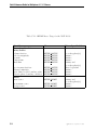
C Quick Reference Guide for Multiphase DEFINE Macros
C-1
C.1 VOF Model . . . . . . . . . . . . . . . . . . . . . . . . . . . . . . . . . . C-1
C.2 Mixture Model . . . . . . . . . . . . . . . . . . . . . . . . . . . . . . . . C-4
C.3 Eulerian Model - Laminar Flow . . . . . . . . . . . . . . . . . . . . . . . C-7
C.4 Eulerian Model - Mixture Turbulence Flow . . . . . . . . . . . . . . . . C-11
C.5 Eulerian Model - Dispersed Turbulence Flow . . . . . . . . . . . . . . . . C-14
C.6 Eulerian Model - Per Phase Turbulence Flow . . . . . . . . . . . . . . . C-18
c Fluent Inc. September 11, 2006
xi
CONTENTS
xii
c Fluent Inc. September 11, 2006
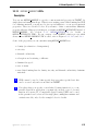
About This Document
User-defined functions (UDFs) allow you to customize FLUENT and can significantly
enhance its capabilities. This UDF Manual presents detailed information on how to
write, compile, and use UDFs in FLUENT. Examples have also been included, where
available. General information about C programming basics is included in an appendix.
Information in this manual is presented in the following chapters:
• Chapter 1: Overview
• Chapter 2: DEFINE Macros
• Chapter 3: Additional Macros for Writing UDFs
• Chapter 4: Interpreting UDFs
• Chapter 5: Compiling UDFs
• Chapter 6: Hooking UDFs to FLUENT
• Chapter 7: Parallel Considerations
• Chapter 8: Examples
This document provides some basic information about the C programming language
(Appendix A) as it relates to user-defined functions in FLUENT, and assumes that
you are an experienced programmer in C. If you are unfamiliar with C, please
consult a C language reference guide (e.g., [2, 3]) before you begin the process of
writing UDFs and using them in your FLUENT model.
This document does not imply responsibility on the part of Fluent Inc. for the accuracy or stability of solutions obtained using UDFs that are either user-generated
or provided by Fluent Inc. Support for current license holders will be limited to
guidance related to communication between a UDF and the FLUENT solver. Other
aspects of the UDF development process that include conceptual function design,
implementation (writing C code), compilation and debugging of C source code, execution of the UDF, and function design verification will remain the responsibility
of the UDF author.
UDF compiled libraries are specific to the computer architecture being used and the
version of the FLUENT executable being run and must be rebuilt any time FLUENT
is upgraded, your operating system changes, or the job is run on a different type of
computer. Note that UDFs may need to be updated with new versions of FLUENT.
c Fluent Inc. September 11, 2006
i
About This Document
ii
c Fluent Inc. September 11, 2006
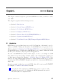
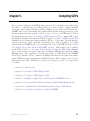
Chapter 1.
Overview
This chapter contains an overview of user-defined functions (UDFs) and their usage in
FLUENT. Details about UDF functionality are described in the following sections:
• Section 1.1: What is a User-Defined Function (UDF)?
• Section 1.2: Why Use UDFs?
• Section 1.3: Limitations
• Section 1.4: Defining Your UDF Using DEFINE Macros
• Section 1.5: Interpreting and Compiling UDFs
• Section 1.6: Hooking UDFs to Your FLUENT Model
• Section 1.7: Grid Terminology
• Section 1.8: Data Types in FLUENT
• Section 1.9: UDF Calling Sequence in the Solution Process
• Section 1.10: Special Considerations for Multiphase UDFs
1.1
What is a User-Defined Function (UDF)?
A user-defined function, or UDF, is a function that you program that can be dynamically
loaded with the FLUENT solver to enhance the standard features of the code. For example, you can use a UDF to define your own boundary conditions, material properties,
and source terms for your flow regime, as well as specify customized model parameters
(e.g., DPM, multiphase models), initialize a solution, or enhance post-processing. See
Section 1.2: Why Use UDFs? for more examples.
UDFs are written in the C programming language using any text editor and the source
code file is saved with a .c extension (e.g., myudf.c). One source file can contain a single
UDF or multiple UDFs, and you can define multiple source files. See Appendix A for
some basic information on C programming.
c Fluent Inc. September 11, 2006
1-1
Overview
UDFs are defined using DEFINE macros provided by Fluent Inc (see Chapter 2: DEFINE
Macros). They are coded using additional macros and functions also supplied by Fluent
Inc. that acccess FLUENT solver data and perform other tasks. See Chapter 3: Additional
Macros for Writing UDFs for details.
Every UDF must contain the udf.h file inclusion directive (#include "udf.h") at the
beginning of the source code file, which allows definitions of DEFINE macros and other
Fluent-provided macros and functions to be included during the compilation process.
See Section 1.4.1: Including the udf.h Header File in Your Source File for details. Note
that values that are passed to a solver by a UDF or returned by the solver to a UDF are
specified in SI units.
Source files containing UDFs can be either interpreted or compiled in FLUENT. For interpreted UDFs, source files are interpreted and loaded directly at runtime, in a single-step
process. For compiled UDFs, the process involves two separate steps. A shared object
code library is first built and then it is loaded into FLUENT. See Chapter 4: Interpreting
UDFs and Chapter 5: Compiling UDFs. Once interpreted or compiled, UDFs will become visible and selectable in FLUENT graphics panels, and can be hooked to a solver
by choosing the function name in the appropriate panel. This process is described in
Chapter 6: Hooking UDFs to FLUENT.
In summary, UDFs:
• are written in the C programming language. (Appendix A)
• must have an include statement for the udf.h file. (Section 1.4.1: Including the
udf.h Header File in Your Source File)
• must be defined using DEFINE macros supplied by Fluent Inc. (Chapter 2: DEFINE
Macros)
• utilize predfined macros and functions supplied by Fluent Inc. to acccess FLUENT
solver data and perform other tasks. (Chapter 3: Additional Macros for Writing
UDFs)
• are executed as interpreted or compiled functions. (Chapter 4: Interpreting UDFs
and Chapter 5: Compiling UDFs)
• are hooked to a FLUENT solver using a graphical user interface panel. (Chapter 6: Hooking UDFs to FLUENT)
• use and return values specified in SI units.
1-2
c Fluent Inc. September 11, 2006
1.2 Why Use UDFs?
1.2
Why Use UDFs?
UDFs allow you to customize FLUENT to fit your particular modeling needs. UDFs can
be used for a variety of applications, some examples of which are listed below.
• Customization of boundary conditions, material property definitions, surface and
volume reaction rates, source terms in FLUENT transport equations, source terms
in user-defined scalar (UDS) transport equations, diffusivity functions, etc.
• Adjustment of computed values on a once-per-iteration basis.
• Initialization of a solution.
• Asynchronous (on demand) execution of a UDF
• Execution at the end of an iteration, upon exit from FLUENT, or upon loading of
a compiled UDF library.
• Post-processing enhancement.
• Enhancement of existing FLUENT models (e.g., discrete phase model, multiphase
mixture model, discrete ordinates radiation model).
Simple examples of UDFs that demonstrate usage are provided with most DEFINE macro
descriptions in Chapter 2: DEFINE Macros). In addition, a step-by-step example (minitutorial) and detailed examples can be found in Chapter 8: Examples.
1.3
Limitations
Although the UDF capability in FLUENT can address a wide range of applications, it
is not possible to address every application using UDFs. Not all solution variables or
FLUENT models can be accessed by UDFs. Specific heat values, for example, cannot be
modified; this would require additional solver capabilities. If you are unsure whether a
particular problem can be handled using a UDF, you can contact your technical support
engineer for assistance.
i
Note that you may need to update your UDF when using a new version of
FLUENT.
c Fluent Inc. September 11, 2006
1-3
Overview
1.4
Defining Your UDF Using DEFINE Macros
UDFs are defined using Fluent-supplied function declarations. These function declarations are implemented in the code as macros, and are referred to in this document as
DEFINE (all capitals) macros. Definitions for DEFINE macros are contained in the udf.h
header file (see Appendix B for a listing). For a complete description of each DEFINE
macro and an example of its usage, refer to Chapter 2: DEFINE Macros.
The general format of a DEFINE macro is
DEFINE_MACRONAME(udf_name, passed-in variables)
where the first argument in the parentheses is the name of the UDF that you supply.
Name arguments are case-sensitive and must be specified in lowercase. The name that you
choose for your UDF will become visible and selectable in drop-down lists in graphical
user-interface panels in FLUENT, once the function has been interpreted or compiled.
The second set of input arguments to the DEFINE macro are variables that are passed
into your function from the FLUENT solver.
For example, the macro
DEFINE_PROFILE(inlet_x_velocity, thread, index)
defines a boundary profile function named inlet x velocity with two variables, thread
and index, that are passed into the function from FLUENT. These passed-in variables are
the boundary condition zone ID (as a pointer to the thread) and the index identifying
the variable that is to be stored. Once the UDF has been interpreted or compiled, its
name (e.g., inlet x velocity) will become visible and selectable in drop-down lists in
the appropriate boundary condition panel (e.g., Velocity Inlet) in FLUENT.
1-4
i
Note that all of the arguments to a DEFINE macro need to be placed on the
same line in your source code. Splitting the DEFINE statement onto several
lines will result in a compilation error.
i
Do not include a DEFINE macro statement (e.g., DEFINE PROFILE) within
a comment in your source code. This will cause a compilation error.
c Fluent Inc. September 11, 2006
1.4 Defining Your UDF Using DEFINE Macros
1.4.1
Including the udf.h Header File in Your Source File
The udf.h header file contains definitions for DEFINE macros as well as #include compiler
directives for C library function header files. It also includes header files (e.g., mem.h) for
other Fluent-supplied macros and functions. You must, therefore, include the udf.h file
at the beginning of every UDF source code file using the #include compiler directive:
#include "udf.h"
For example, when udf.h is included in the source file containing the DEFINE statement
from the previous section,
#include "udf.h"
DEFINE_PROFILE(inlet_x_velocity, thread, index)
upon compilation, the macro will expand to
void inlet_x_velocity(Thread *thread, int index)
i
You won’t need to put a copy of udf.h in your local directory when you compile your UDF. The FLUENT solver
automatically reads the udf.h file from the Fluent.Inc/
fluent6.x/src/ directory once your UDF is compiled.
c Fluent Inc. September 11, 2006
1-5
Overview
1.5
Interpreting and Compiling UDFs
Source code files containing UDFs can be either interpreted or compiled in FLUENT. In
both cases the functions are compiled, but the way in which the source code is compiled,
and the code that results from the compilation process is different for the two methods.
These differences are explained below.
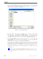
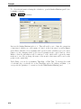
Compiled UDFs
Compiled UDFs are built in the same way that the FLUENT executable itself is built. A
script called Makefile is used to invoke the system C compiler to build an object code
library. You initiate this action in the Compiled UDFs panel by clicking on the Build
pushbutton. The object code library contains the native machine language translation
of your higher-level C source code. The shared library must then loaded into FLUENT at
runtime by a process called “dynamic loading.” You initiate this action in the Compiled
UDFs panel by clicking on the Load pushbutton. The object libraries are specific to the
computer architecture being used, as well as to the particular version of the FLUENT
executable being run. The libraries must, therefore, be rebuilt any time FLUENT is
upgraded, when the computer’s operating system level changes, or when the job is run
on a different type of computer.
In summary, compiled UDFs are compiled from source files using the graphical user
interface, in a two-step process. The process involves a visit to the Compiled UDFs panel
where you first Build shared library object file(s) from a source file, and then Load the
shared library that was just built into FLUENT.
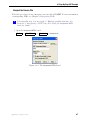
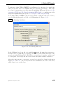
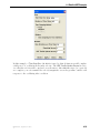
Interpreted UDFs
Interpreted UDFs are interpreted from source files using the graphical user interface, but
in a single-step process. The process, which occurs at runtime, involves a visit to the
Interpreted UDFs panel where you Interpret a source file.
Inside FLUENT, the source code is compiled into an intermediate, architecture-independent
machine code using a C preprocessor. This machine code then executes on an internal
emulator, or interpreter, when the UDF is invoked. This extra layer of code incurs a
performance penalty, but allows an interpreted UDF to be shared effortlessly between
different architectures, operating systems, and FLUENT versions. If execution speed
does become an issue, an interpreted UDF can always be run in compiled mode without
modification.
1-6
c Fluent Inc. September 11, 2006
1.5 Interpreting and Compiling UDFs
The interpreter that is used for interpreted UDFs does not have all of the capabilities of
a standard C compiler (which is used for compiled UDFs). Specifically interpreted UDFs
cannot contain any of the following C programming language elements:
• goto statements
• non ANSI-C prototypes for syntax
• direct data structure references
• declarations of local structures
• unions
• pointers to functions
• arrays of functions
• multi-dimensional arrays
1.5.1
Differences Between Interpreted and Compiled UDFs
The major difference between interpreted and compiled UDFs is that interpreted UDFs
cannot access FLUENT solver data using direct structure references; they can only indirectly access data through the use of Fluent-supplied macros. This can be significant if,
for example, you want to introduce new data structures in your UDF.
A summary of the differences between interpreted and compiled UDFs is presented below.
See Chapters 4 and 5 for details on interpreting and compiling UDFs, respectively, in
FLUENT.
• Interpreted UDFs
– are portable to other platforms.
– can all be run as compiled UDFs.
– do not require a C compiler.
– are slower than compiled UDFs.
– are restricted in the use of the C programming language.
– cannot be linked to compiled system or user libraries.
– can access data stored in a FLUENT structure only using a predefined macro
(see Chapters 3).
c Fluent Inc. September 11, 2006
1-7
Overview
• Compiled UDFs
– execute faster than interpreted UDFs.
– are not restricted in the use of the C programming language.
– can call functions written in other languages (specifics are system- and compilerdependent).
– cannot necessarily be run as interpreted UDFs if they contain certain elements
of the C language that the interpreter cannot handle.
In summary, when deciding which type of UDF to use for your FLUENT model
• use interpreted UDFs for small, straightforward functions.
• use compiled UDFs for complex functions that
– have a significant CPU requirement (e.g., a property UDF that is called on a
per-cell basis every iteration).
– require access to a shared library.
1.6
Hooking UDFs to Your FLUENT Model
Once your UDF source file is interpreted or compiled, the function(s) contained in the
interpreted code or shared library will appear in drop-down lists in graphical interface
panels, ready for you to activate or “hook” to your CFD model. See Chapter 6: Hooking
UDFs to FLUENT for details on how to hook a UDF to FLUENT.
1.7
Grid Terminology
Most user-defined functions access data from a FLUENT solver. Since solver data is
defined in terms of grid components, you will need to learn some basic grid terminology
before you can write a UDF.
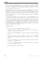
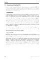
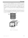
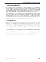
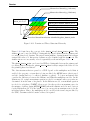
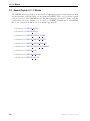
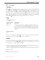
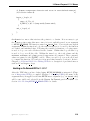
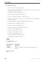
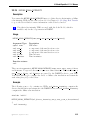
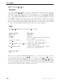
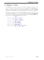
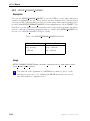
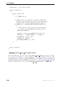
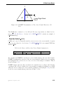
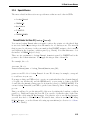
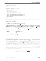
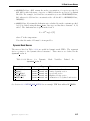
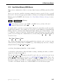
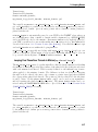
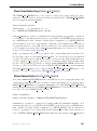
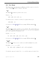
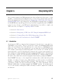
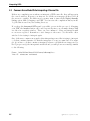
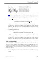
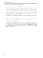
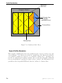
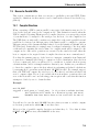
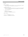
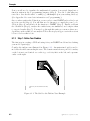
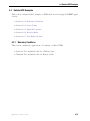
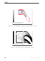
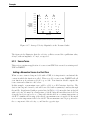
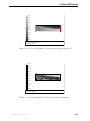
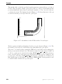
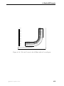
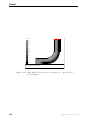
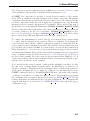
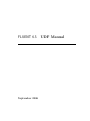
A mesh is broken up into control volumes, or cells. Each cell is defined by a set of grid
points (or nodes), a cell center, and the faces that bound the cell (Figure 1.7.1). FLUENT
uses internal data structures to define the domain(s) of the mesh, to assign an order to
cells, cell faces, and grid points in a mesh, and to establish connectivity between adjacent
cells.
1-8
c Fluent Inc. September 11, 2006
1.7 Grid Terminology
A thread is a data structure in FLUENT that is used to store information about a boundary or cell zone. Cell threads are groupings of cells, and face threads are groupings of
faces. Pointers to thread data structures are often passed to functions and manipulated in
FLUENT to access the information about the boundary or cell zones represented by each
thread. Each boundary or cell zone that you define in your FLUENT model in a boundary conditions panel has an integer Zone ID that is associated with the data contained
within the zone. You won’t see the term “thread” in a graphics panel in FLUENT so you
can think of a ’zone’ as being the same as a ’thread’ data structure when programming
UDFs.
Cells and cell faces are grouped into zones that typically define the physical components
of the model (e.g., inlets, outlets, walls, fluid regions). A face will bound either one or
two cells depending on whether it is a boundary face or an interior face. A domain is a
data structure in FLUENT that is used to store information about a collection of node,
face threads, and cell threads in a mesh.
* node
*
cell
center
face
cell
simple 2D grid
nodes
*
*
*
*
*
*
*
edge
face
cell
simple 3D grid
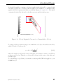
Figure 1.7.1: Grid Components
c Fluent Inc. September 11, 2006
1-9
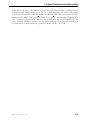
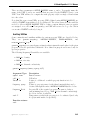
Overview
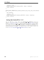
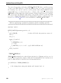
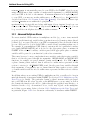
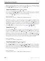
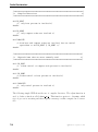
node
node thread
edge
face
face thread
cell
cell center
cell thread
domain
grid point
grouping of nodes
boundary of a face (3D)
boundary of a cell (2D or 3D)
grouping of faces
control volume into which domain is broken up
location where cell data is stored
grouping of cells
a grouping of node, face, and cell threads
1.8 Data Types in FLUENT
In addition to standard C language data types such as real, int, etc. that can be used to
define data in your UDF, there are FLUENT-specific data types that are associated with
solver data. These data types represent the computational units for a grid (Figure 1.7.1).
Variables that are defined using these data types are typically supplied as arguments to
DEFINE macros as well as to other special functions that access FLUENT solver data.
Some of the more commonly-used FLUENT data types are:
Node
face t
cell t
Thread
Domain
Node is a structure data type that stores data associated with a grid point.
face t is an integer data type that identifies a particular face within a face thread.
cell t is an integer data type that identifies a particular cell within a cell thread.
Thread is a structure data type that stores data that is common to the group of cells or
faces that it represents. For multiphase applications, there is a thread structure for each
phase, as well as for the mixture. See Section 1.10.1: Multiphase-specific Data Types for
details.
Domain is a structure data type that stores data associated with a collection of node, face,
and cell threads in a mesh. For single-phase applications, there is only a single domain
structure. For multiphase applications, there are domain structures for each phase, the
interaction between phases, as well as for the mixture. The mixture-level domain is the
highest-level structure for a multiphase model. See Section 1.10.1: Multiphase-specific
Data Types for details.
i
1-10
Note that all of the FLUENT data types are case-sensitive.
c Fluent Inc. September 11, 2006
1.8 Data Types in FLUENT
When you use a UDF in FLUENT, your function can access solution variables at individual
cells or cell faces in the fluid and boundary zones. UDFs need to be passed appropriate
arguments such as a thread reference (i.e., pointer to a particular thread) and the cell
or face ID in order to allow individual cells or faces to be accessed. Note that a face ID
or cell ID, alone, does not uniquely identify the face or cell. A thread pointer is always
required along with the ID to identify which thread the face (or cell) belongs to.
Some UDFs are passed the cell index variable (c) as an argument such as
in DEFINE PROPERTY(my function,c,t), or the face index variable (f) such as in
DEFINE UDS FLUX(my function,f,t,i). If the cell or face index variable(e.g., cell t
c, cell t f) isn’t passed as an argument and is needed in the UDF, the variable is
always available to be used by the function once it has been declared locally. See Section 2.7.3: DEFINE UDS FLUX for an example.
The data structures that are passed to your UDF (as pointers) depend on the DEFINE
macro you are using and the property or term you are trying to modify. For example,
DEFINE ADJUST UDFs are general-purpose functions that are passed a domain pointer
(d) such as in DEFINE ADJUST(my function, d). DEFINE PROFILE UDFs are passed
a thread pointer (t) to the boundary zone that the function is hooked to, such as in
DEFINE PROFILE(my function, thread, i).
Some UDFs, such as DEFINE ON DEMAND functions, aren’t passed any pointers to data
structures while others aren’t passed the pointer the UDF needs. If your UDF needs
to access a thread or domain pointer that is not directly passed by the solver through
an argument, then you will need to use a special Fluent-supplied macro to obtain the
pointer in your UDF. For example, DEFINE ADJUST is passed only the domain pointer
so if your UDF needs a thread pointer, it will have to declare the variable locally and
then obtain it using the special macro Lookup Thread. An exception to this is if your
UDF needs a thread pointer to loop over all of the cell threads or all the face threads
in a domain (using thread c loop(c,t) or thread f loop(f,t), respectively) and the
DEFINE macro isn’t passed it. Since the UDF will be looping over all threads in the
domain, you won’t need to use Lookup Thread to get the thread pointer to pass it to the
looping macro; you’ll just need to declare the thread pointer (and cell or face ID) locally
before calling the loop. See Section 2.2.1: DEFINE ADJUST for an example.
As another example, if you are using DEFINE ON DEMAND (which isn’t passed any pointer
argument) to execute an asynchronous UDF and your UDF needs a domain pointer,
then the function will need to declare the domain variable locally and obtain it using Get Domain. See Section 2.2.8: DEFINE ON DEMAND for an example. Refer to Section 3.2.6: Special Macros for details.
c Fluent Inc. September 11, 2006
1-11
Overview
1.9
UDF Calling Sequence in the Solution Process
UDFs are called at predetermined times in the FLUENT solution process. However,
they can also be executed asynchronously (or “on demand”) using a DEFINE ON DEMAND
UDF. If a DEFINE EXECUTE AT END UDF is utilized, then FLUENT calls the function at
the end of an iteration. A DEFINE EXECUTE AT EXIT is called at the end of a FLUENT
session while a DEFINE EXECUTE ON LOADING is called whenever a UDF compiled library
is loaded. Understanding the context in which UDFs are called within FLUENT’s solution
process may be important when you begin the process of writing UDF code, depending
on the type of UDF you are writing. The solver contains call-outs that are linked to
user-defined functions that you write. Knowing the sequencing of function calls within
an iteration in the FLUENT solution process can help you determine which data are
current and available at any given time.
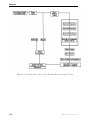
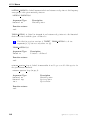
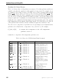
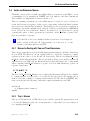
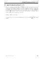
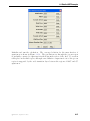
Pressure-Based Segregated Solver
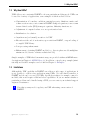
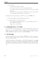
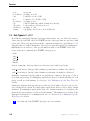
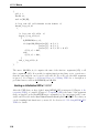
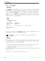
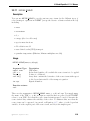
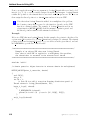
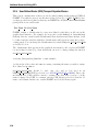
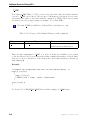
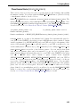
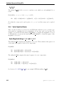
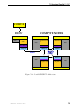
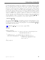
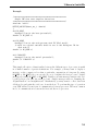
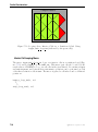
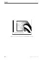
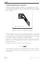
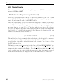
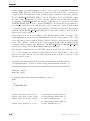
The solution process for the pressure-based segregated solver (Figure 1.9.1) begins with a
two-step initialization sequence that is executed outside the solution iteration loop. This
sequence begins by initializing equations to user-entered (or default) values taken from
the FLUENT user interface. Next, PROFILE UDFs are called followed by a call to INIT
UDFs. Initialization UDFs overwrite initialization values that were previously set.
The solution iteration loop begins with the execution of ADJUST UDFs. Next, momentum
equations for u, v, and w velocities are solved sequentially, followed by mass continuity
and velocity updates. Subsequently, the energy and species equations are solved followed
by turbulence and other scalar transport equations, as required. Note that PROFILE
and SOURCE UDFs are called by each “Solve” routine for the variable currently under
consideration (e.g., species, velocity).
After the conservation equations, properties are updated including PROPERTY UDFs.
Thus, if your model involves the gas law, for example, the density will be updated at
this time using the updated temperature (and pressure and/or species mass fractions).
A check for either convergence or additional requested iterations is done, and the loop
either continues or stops.
1-12
c Fluent Inc. September 11, 2006
1.9 UDF Calling Sequence in the Solution Process
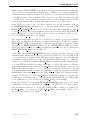
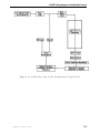
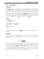
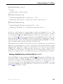
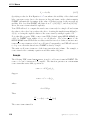
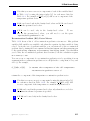
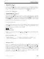
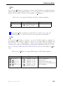
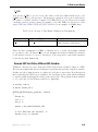
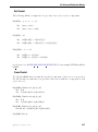
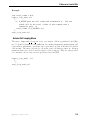
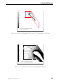
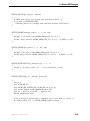
Pressure-Based Coupled Solver
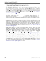
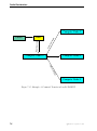
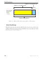
The solution process for the pressure-based coupled solver (Figure 1.9.2) begins with a
two-step initialization sequence that is executed outside the solution iteration loop. This
sequence begins by initializing equations to user-entered (or default) values taken from
the FLUENT user interface. Next, PROFILE UDFs are called followed by a call to INIT
UDFs. Initialization UDFs overwrite initialization values that were previously set.
The solution iteration loop begins with the execution of ADJUST UDFs. Next, FLUENT
solves the governing equations of continuity and momentum in a coupled fashion, which
is simultaneously as a set, or vector, of equations. Energy, species tranpsort, turbulence,
and other transport equations as required are subsequently solved sequentially, and the
remaining process is the same as the pressure-based segregated solver.
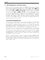
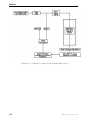
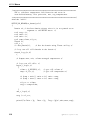
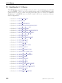
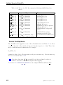
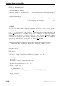
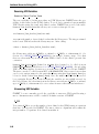
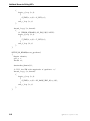
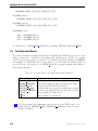
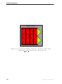
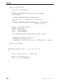
Density-Based Solver
As is the case for the other solvers, the solution process for the density-based solver
(Figure 1.9.3) begins with a two-step initialization sequence that is executed outside the
solution iteration loop. This sequence begins by initializing equations to user-entered (or
default) values taken from the FLUENT user interface. Next, PROFILE UDFs are called
followed by a call to INIT UDFs. Initialization UDFs overwrite initialization values that
were previously set.
The solution iteration loop begins with the execution of ADJUST UDFs. Next, FLUENT
solves the governing equations of continuity and momentum, energy, and species transport in a coupled fashion, which is simultaneously as a set, or vector, of equations. Turbulence and other transport equations as required are subsequently solved sequentially,
and the remaining process is the same as the pressure-based segregated solver.
c Fluent Inc. September 11, 2006
1-13
Overview
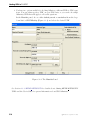
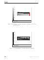
Figure 1.9.1: Solution Procedure for the Pressure-Based Segregated Solver
1-14
c Fluent Inc. September 11, 2006
1.9 UDF Calling Sequence in the Solution Process
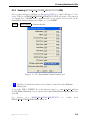
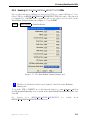
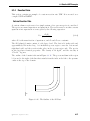
Figure 1.9.2: Solution Procedure for the Pressure-Based Coupled Solver
c Fluent Inc. September 11, 2006
1-15
Overview
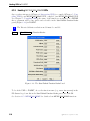
Figure 1.9.3: Solution Procedure for the Density-Based Solver
1-16
c Fluent Inc. September 11, 2006
1.10 Special Considerations for Multiphase UDFs
1.10 Special Considerations for Multiphase UDFs
In many cases, the UDF source code that you will write for a single-phase flow will be
the same as for a multiphase flow. For example, there will be no differences between
the C code for a single-phase boundary profile (defined using DEFINE PROFILE) and the
code for a multiphase profile, assuming that the function is accessing data only from the
phase-level domain that it is hooked to in the graphical user interface. If your UDF is
not explicitly passed a pointer to the thread or domain structure that it requires, you will
need to use a special multiphase-specific macro (e.g., THREAD SUB THREAD) to retrieve it.
This is discussed in Chapter 3: Additional Macros for Writing UDFs.
See Appendix B for a complete list of general-purpose DEFINE macros and multiphasespecific DEFINE macros that can be used to define UDFs for multiphase model cases.
1.10.1
Multiphase-specific Data Types
In addition to the FLUENT-specific data types presented in Section 1.8: Data Types
in FLUENT, there are special thread and domain data structures that are specific to
multiphase UDFs. These data types are used to store properties and variables for the
mixture of all of the phases, as well as for each individual phase when a multiphase model
(i.e., Mixture, VOF, Eulerian) is used.
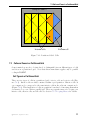
In a multiphase application, the top-level domain is referred to as the ’superdomain’.
Each phase occupies a domain referred to as a ’subdomain’. A third domain type,
the ’interaction’ domain, is introduced to allow for the definition of phase interaction
mechanisms. When mixture properties and variables are needed (a sum over phases),
the superdomain is used for those quantities while the subdomain carries the information
for individual phases. In single-phase, the concept of a mixture is used to represent the
sum over all the species (components) while in multiphase it represents the sum over all
the phases. This distinction is important since FLUENT has the capability of handling
multiphase multi-components, where, for example, a phase can consist of a mixture of
species.
Since solver information is stored in thread data structures, threads must be associated
with the superdomain as well as with each of the subdomains. In other words, for each
cell or face thread defined in the superdomain, there is a corresponding cell or face
thread defined for each subdomain. Some of the information defined in one thread of
the superdomain is shared with the corresponding threads of each of the subdomains.
Threads associated with the superdomain are referred to as ’superthreads’, while threads
associated with the subdomain are referred to as phase-level threads, or ’subthreads’.
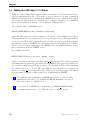
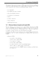
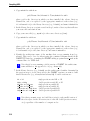
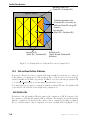
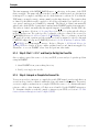
The domain and thread hierarchy are summarized in Figure 1.10.1.
c Fluent Inc. September 11, 2006
1-17
Overview
Mixture-level thread (e.g., inlet zone)
Mixture-level thread (e.g., fluid zone)
Mixture domain, domain_id = 1
Interaction domains
domain_id = 5, 6, 7
0
0
Primary phase domain, domain_id = 2
1
1
Secondary phase domain, domain_id = 3
2
2
Secondary phase domain, domain_id = 4
Phase-level threads for inlet zone identified by phase_domain_index
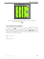
Figure 1.10.1: Domain and Thread Structure Hierarchy
Figure 1.10.1 introduces the concept of the domain id and phase domain index. The
domain id can be used in UDFs to distinguish the superdomain from the primary and
secondary phase-level domains. The superdomain (mixture domain) domain id is always
assigned the value of 1. Interaction domains are also identified with the domain id. The
domain ids are not necessarily ordered sequentially as shown in Figure 1.10.1.
The phase domain index can be used in UDFs to distinguish between the primary and
secondary phase-level threads. phase domain index is always assigned the value of 0 for
the primary phase-level thread.
The data structures that are passed to a UDF depend on the multiphase model that is
enabled, the property or term that is being modified, the DEFINE macro that is used,
and the domain that is to be affected (mixture or phase). To better understand this,
consider the differences between the Mixture and Eulerian multiphase models. In the
Mixture model, a single momentum equation is solved for a mixture whose properties are
determined from the sum of its phases. In the Eulerian model, a momentum equation
is solved for each phase. FLUENT allows you to directly specify a momentum source for
the mixture of phases (using DEFINE SOURCE) when the mixture model is used, but not
for the Eulerian model. For the latter case, you can specify momentum sources for the
individual phases. Hence, the multiphase model, as well as the term being modified by
the UDF, determines which domain or thread is required.
1-18
c Fluent Inc. September 11, 2006
1.10 Special Considerations for Multiphase UDFs
UDFs that are hooked to the mixture of phases are passed superdomain (or mixture-level)
structures, while functions that are hooked to a particular phase are passed subdomain
(or phase-level) structures. DEFINE ADJUST and DEFINE INIT UDFs are hardwired to the
mixture-level domain. Other types of UDFs are hooked to different phase domains. For
your convenience, Appendix B contains a list of multiphase models in FLUENT and the
phase on which UDFs are specified for the given variables. From this information, you
can infer which domain structure is passed from the solver to the UDF.
c Fluent Inc. September 11, 2006
1-19
Overview
1-20
c Fluent Inc. September 11, 2006
Chapter 2.
DEFINE Macros
This chapter contains descriptions of predefined DEFINE macros that you will use to define
your UDF.
The chapter is organized in the following sections:
• Section 2.1: Introduction
• Section 2.2: General Purpose DEFINE Macros
• Section 2.3: Model-Specific DEFINE Macros
• Section 2.4: Multiphase DEFINE Macros
• Section 2.5: Discrete Phase Model (DPM) DEFINE Macros
• Section 2.6: Dynamic Mesh DEFINE Macros
• Section 2.7: User-Defined Scalar (UDS) Transport Equation DEFINE Macros
2.1
Introduction
DEFINE macros are predefined macros provided by Fluent Inc. that must be used to
define your UDF. A listing and discussion of each DEFINE macros is presented below.
(Refer to Section 1.4: Defining Your UDF Using DEFINE Macros for general information
about DEFINE macros.) Definitions for DEFINE macros are contained within the udf.h
file. For your convenience, they are provided in Appendix B.
For each of the DEFINE macros listed in this chapter, a source code example of a UDF
that utilizes it is provided, where available. Many of the examples make extensive use
of other macros presented in Chapter 3: Additional Macros for Writing UDFs. Note
that not all of the examples in the chapter are complete functions that can be executed
as stand-alone UDFs in FLUENT. Examples are intended to demonstrate DEFINE macro
usage only.
Special care must be taken for some serial UDFs that will be run in parallel FLUENT.
See Chapter 7: Parallel Considerations for details.
i
Note that all of the arguments to a DEFINE macro need to be placed on the
same line in your source code. Splitting the DEFINE statement onto several
lines will result in a compilation error.
c Fluent Inc. September 11, 2006
2-1
DEFINE Macros
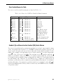
2.2
General Purpose DEFINE Macros
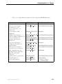
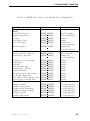
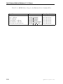
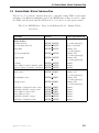
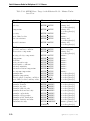
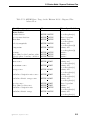
The DEFINE macros presented in this section implement general solver functions that
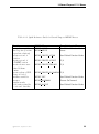
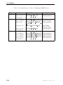
are independent of the model(s) you are using in FLUENT. Table 2.2.1 provides a quick
reference guide to these DEFINE macros, the functions they are used to define, and the
panels where they are activated or “hooked” to FLUENT. Definitions of each DEFINE
macro are contained in udf.h can be found in Appendix B.
• Section 2.2.1: DEFINE ADJUST
• Section 2.2.2: DEFINE DELTAT
• Section 2.2.3: DEFINE EXECUTE AT END
• Section 2.2.4: DEFINE EXECUTE AT EXIT
• Section 2.2.5: DEFINE EXECUTE FROM GUI
• Section 2.2.6: DEFINE EXECUTE ON LOADING
• Section 2.2.7: DEFINE INIT
• Section 2.2.8: DEFINE ON DEMAND
• Section 2.2.9: DEFINE RW FILE
2-2
c Fluent Inc. September 11, 2006
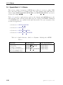
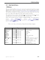
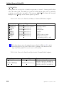
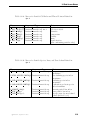
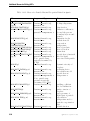
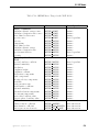
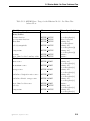
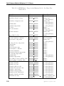
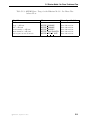
2.2 General Purpose DEFINE Macros
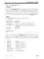
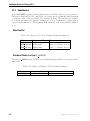
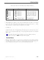
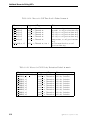
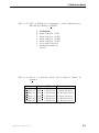
Table 2.2.1: Quick Reference Guide for General Purpose DEFINE Macros
Function
manipulates variables
time step size (for time
dependent solutions)
executes at end of
iteration
executes at end of
a FLUENT session
executes from a userdefined Scheme
routine
executes when a UDF
library is loaded
initializes variables
executes
asynchronously
reads/writes variables
to case and data files
c Fluent Inc. September 11, 2006
DEFINE Macro
DEFINE ADJUST
DEFINE DELTAT
Panel Activated In
User-Defined Function Hooks
Iterate
DEFINE EXECUTE AT END
User-Defined Function Hooks
DEFINE EXECUTE AT EXIT
N/A
DEFINE EXECUTE FROM GUI
N/A
DEFINE EXECUTE ON LOADING N/A
DEFINE INIT
DEFINE ON DEMAND
User-Defined Function Hooks
Execute On Demand
DEFINE RW FILE
User-Defined Function Hooks
2-3
DEFINE Macros
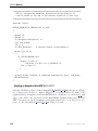
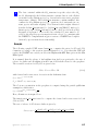
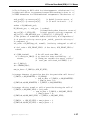
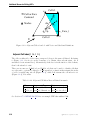
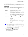
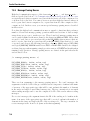
2.2.1 DEFINE ADJUST
Description
DEFINE ADJUST is a general-purpose macro that can be used to adjust or modify FLUENT
variables that are not passed as arguments. For example, you can use DEFINE ADJUST to
modify flow variables (e.g., velocities, pressure) and compute integrals. You can also use
it to integrate a scalar quantity over a domain and adjust a boundary condition based on
the result. A function that is defined using DEFINE ADJUST executes at every iteration
and is called at the beginning of every iteration before transport equations are solved.
For an overview of the FLUENT solution process which shows when a DEFINE ADJUST
UDF is called, refer to Figures 1.9.1, 1.9.2, and 1.9.3.
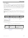
Usage
DEFINE ADJUST(name,d)
Argument Type
symbol name
Domain *d
Description
UDF name.
Pointer to the domain over which the adjust function is
to be applied. The domain argument provides access to all
cell and face threads in the mesh. For multiphase flows, the
pointer that is passed to the function by the solver is the
mixture-level domain.
Function returns
void
There are two arguments to DEFINE ADJUST: name and d. You supply name, the name of
the UDF. d is passed by the FLUENT solver to your UDF.
2-4
c Fluent Inc. September 11, 2006
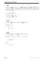
2.2 General Purpose DEFINE Macros
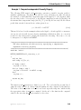
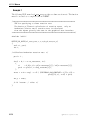
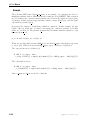
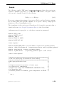
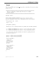
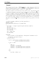
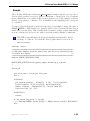
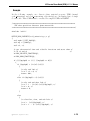
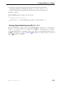
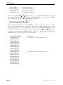
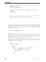
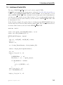
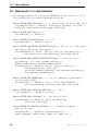
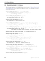
Example 1
The following UDF, named my adjust, integrates the turbulent dissipation over the
entire domain using DEFINE ADJUST. This value is then printed to the console window.
The UDF is called once every iteration. It can be executed as an interpreted or compiled
UDF in FLUENT.
/********************************************************************
UDF for integrating turbulent dissipation and printing it to
console window
*********************************************************************/
#include "udf.h"
DEFINE_ADJUST(my_adjust,d)
{
Thread *t;
/* Integrate dissipation. */
real sum_diss=0.;
cell_t c;
thread_loop_c(t,d)
{
begin_c_loop(c,t)
sum_diss += C_D(c,t)*
C_VOLUME(c,t);
end_c_loop(c,t)
}
printf("Volume integral of turbulent dissipation: %g\n", sum_diss);
}
c Fluent Inc. September 11, 2006
2-5
DEFINE Macros
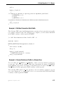
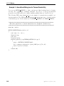
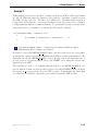
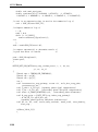
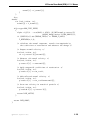
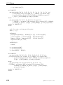
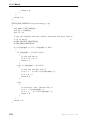
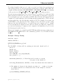
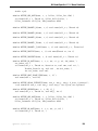
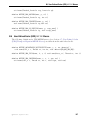
Example 2
The following UDF, named adjust fcn, specifies a user-defined scalar as a function of
the gradient of another user-defined scalar, using DEFINE ADJUST. The function is called
once every iteration. It is executed as a compiled UDF in FLUENT.
/********************************************************************
UDF for defining user-defined scalars and their gradients
*********************************************************************/
#include "udf.h"
DEFINE_ADJUST(adjust_fcn,d)
{
Thread *t;
cell_t c;
real K_EL = 1.0;
/* Do nothing if gradient isn’t allocated yet. */
if (! Data_Valid_P())
return;
thread_loop_c(t,d)
{
if (FLUID_THREAD_P(t))
{
begin_c_loop_all(c,t)
{
C_UDSI(c,t,1) +=
K_EL*NV_MAG2(C_UDSI_G(c,t,0))*C_VOLUME(c,t);
}
end_c_loop_all(c,t)
}
}
}
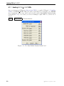
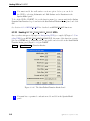
Hooking an Adjust UDF to FLUENT
After the UDF that you have defined using DEFINE ADJUST is interpreted (Chapter 4: Interpreting UDFs) or compiled (Chapter 5: Compiling UDFs), the name of the argument
that you supplied as the first DEFINE macro argument (e.g., adjust fcn) will become visible and selectable in the User-Defined Function Hooks panel in FLUENT. Note that you can
hook multiple adjust functions to your model. See Section 6.1.1: Hooking DEFINE ADJUST
UDFs for details.
2-6
c Fluent Inc. September 11, 2006
2.2 General Purpose DEFINE Macros
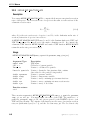
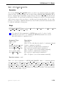
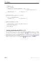
2.2.2 DEFINE DELTAT
Description
DEFINE DELTAT is a general-purpose macro that you can use to control the size of the
time step during the solution of a time-dependent problem. Note that this macro can be
used only if the adaptive time-stepping method option has been activated in the Iterate
panel in FLUENT.
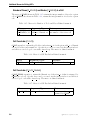
Usage
DEFINE DELTAT(name,d)
Argument Type
symbol name
Domain *d
Description
UDF name.
Pointer to domain over which the time stepping control
function is to be applied. The domain argument provides access
to all cell and face threads in the mesh. For multiphase flows,
the pointer that is passed to the function by the solver is the
mixture-level domain.
Function returns
real
There are two arguments to DEFINE DELTAT: name and domain. You supply name, the
name of the UDF. domain is passed by the FLUENT solver to your UDF. Your UDF will
need to compute the real value of the physical time step and return it to the solver.
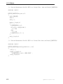
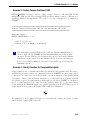
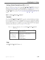
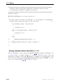
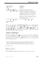
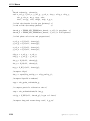
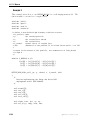
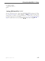
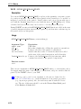
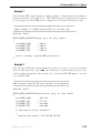
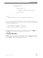
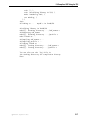
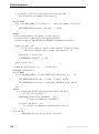
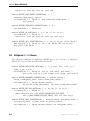
Example
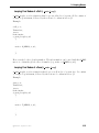
The following UDF, named mydeltat, is a simple function that shows how you can use
DEFINE DELTAT to change the value of the time step in a simulation. First, CURRENT TIME
is used to get the value of the current simulation time (which is assigned to the variable
flow time). Then, for the first 0.5 seconds of the calculation, a time step of 0.1 is set.
A time step of 0.2 is set for the remainder of the simulation. The time step variable
is then returned to the solver. See Section 3.5: Time-Dependent Macros for details on
CURRENT TIME.
c Fluent Inc. September 11, 2006
2-7
DEFINE Macros
/*********************************************************************
UDF that changes the time step value for a time-dependent solution
**********************************************************************/
#include "udf.h"
DEFINE_DELTAT(mydeltat,d)
{
real time_step;
real flow_time = CURRENT_TIME;
if (flow_time < 0.5)
time_step = 0.1;
else
time_step = 0.2;
return time_step;
}
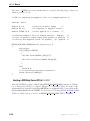
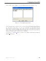
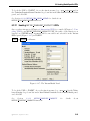
Hooking an Adaptive Time Step UDF to FLUENT
After the UDF that you have defined using DEFINE DELTAT is interpreted (Chapter 4: Interpreting UDFs) or compiled (Chapter 5: Compiling UDFs), the name of the argument
that you supplied as the first DEFINE macro argument (e.g,. mydeltat) will become visible
and selectable in the Iterate panel in FLUENT. See Section 6.1.2: Hooking DEFINE DELTAT
UDFs for details.
2-8
c Fluent Inc. September 11, 2006
2.2 General Purpose DEFINE Macros
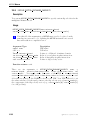
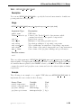
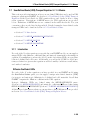
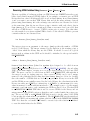
2.2.3 DEFINE EXECUTE AT END
Description
DEFINE EXECUTE AT END is a general-purpose macro that is executed at the end of an
iteration in a steady state run, or at the end of a time step in a transient run. You
can use DEFINE EXECUTE AT END when you want to calculate flow quantities at these
particular times. Note that you do not have to specify whether your execute-at-end
UDF gets executed at the end of a time step or the end of an iteration. This is done
automatically when you select the steady or unsteady time method in your FLUENT
model.
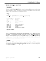
Usage
DEFINE EXECUTE AT END(name)
Argument Type
symbol name
Description
UDF name.
Function returns
void
There is only one argument to DEFINE EXECUTE AT END: name. You supply name, the
name of the UDF. Unlike DEFINE ADJUST, DEFINE EXECUTE AT END is not passed a domain pointer. Therefore, if your function requires access to a domain pointer, then you
will need to use the utility Get Domain(ID) to explicitly obtain it (see Section 3.2.6: Domain Pointer (Get Domain) and the example below). If your UDF requires access to a
phase domain pointer in a multiphase solution, then it will need to pass the appropriate
phase ID to Get Domain in order to obtain it.
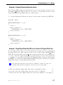
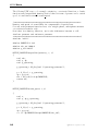
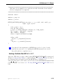
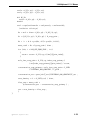
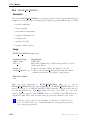
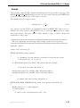
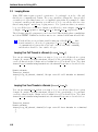
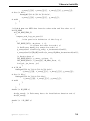
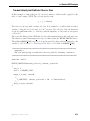
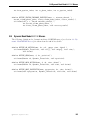
Example
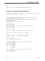
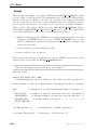
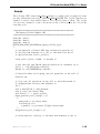
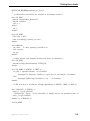
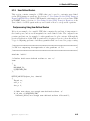
The following UDF, named execute at end, integrates the turbulent dissipation over
the entire domain using DEFINE EXECUTE AT END and prints it to the console window at
the end of the current iteration or time step. It can be executed as an interpreted or
compiled UDF in FLUENT.
c Fluent Inc. September 11, 2006
2-9
DEFINE Macros
/********************************************************************
UDF for integrating turbulent dissipation and printing it to
console window at the end of the current iteration or time step
*********************************************************************/
#include "udf.h"
DEFINE_EXECUTE_AT_END(execute_at_end)
{
Domain *d;
Thread *t;
/* Integrate dissipation. */
real sum_diss=0.;
cell_t c;
d = Get_Domain(1);
/* mixture domain if multiphase */
thread_loop_c(t,d)
{
if (FLUID_THREAD_P(t))
{
begin_c_loop(c,t)
sum_diss += C_D(c,t) * C_VOLUME(c,t);
end_c_loop(c,t)
}
}
printf("Volume integral of turbulent dissipation: %g\n", sum_diss);
fflush(stdout);
}
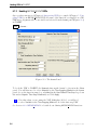
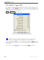
Hooking an Execute-at-End UDF to FLUENT
After the UDF that you have defined using DEFINE EXECUTE AT END is interpreted (Chapter 4: Interpreting UDFs) or compiled (Chapter 5: Compiling UDFs), the name of the
argument that you supplied as the first DEFINE macro argument (e.g. execute at end)
will become visible and selectable in the User-Defined Function Hooks panel in FLUENT. Note that you can hook multiple end-iteration functions to your model. See Section 6.1.3: Hooking DEFINE EXECUTE AT END UDFs for details.
2-10
c Fluent Inc. September 11, 2006
2.2 General Purpose DEFINE Macros
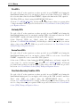
2.2.4 DEFINE EXECUTE AT EXIT
Description
DEFINE EXECUTE AT EXIT is a general-purpose macro that can be used to execute a function at the end of a FLUENT session.
Usage
DEFINE EXECUTE AT EXIT(name)
Argument Type
symbol name
Description
UDF name.
Function returns
void
There is only one argument to DEFINE EXECUTE AT EXIT: name. You supply name, the
name of the UDF.
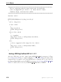
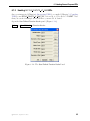
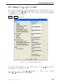
Hooking an Execute-at-Exit UDF to FLUENT
After the UDF that you have defined using DEFINE EXECUTE AT EXIT is interpreted
(Chapter 4: Interpreting UDFs) or compiled (Chapter 5: Compiling UDFs), the name of
the argument that you supplied as the first DEFINE macro argument will become visible and selectable in the User-Defined Function Hooks panel in FLUENT. Note that you can
hook
multiple
at-exit
UDFs
to
your
model.
See Section 6.1.4: Hooking DEFINE EXECUTE AT EXIT UDFs for details.
c Fluent Inc. September 11, 2006
2-11
DEFINE Macros
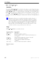
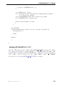
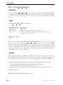
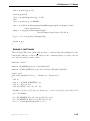
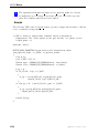
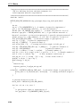
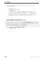
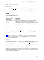
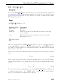
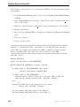
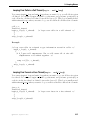
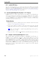
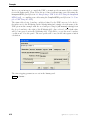
2.2.5 DEFINE EXECUTE FROM GUI
Description
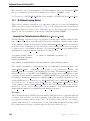
DEFINE EXECUTE FROM GUI is a general-purpose macro that you can use to define a UDF
which is to be executed from a user-defined graphical user interface (GUI). For example,
a C function that is defined using DEFINE EXECUTE FROM GUI can be executed whenever
a button is clicked in a user-defined GUI. Custom GUI components (panels, buttons,
etc.) are defined in FLUENT using the Scheme language.
Usage
DEFINE EXECUTE FROM GUI(name,libname,mode)
Argument Type
symbol name
char *libname
int mode
Description
UDF name.
name of the UDF library that has been loaded in FLUENT
an integer passed from the Scheme program that defines the
user-defined GUI.
Function returns
void
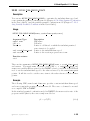
There are three arguments to DEFINE EXECUTE FROM GUI: name, libname, and mode.
You supply name, the name of the UDF. The variables libname and mode are passed by
the FLUENT solver to your UDF. The integer variable mode is passed from the Scheme
program which defines the user-defined GUI, and represent the possible user options
available from the GUI panel. A different C function in UDF can be called for each
option. For example, the user-defined GUI panel may have a number of buttons. Each
button may be represented by different integers, which, when clicked, will execute a
corresponding C function.
i
2-12
DEFINE EXECUTE FROM GUI UDFs must be implemented as compiled UDFs,
and there can be only one function of this type in a UDF library.
c Fluent Inc. September 11, 2006
2.2 General Purpose DEFINE Macros
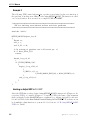
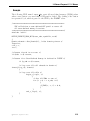
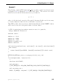
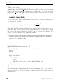
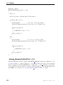
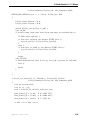
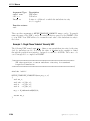
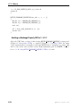
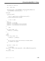
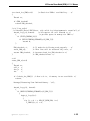
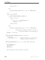
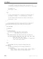
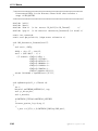
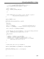
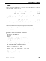
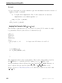
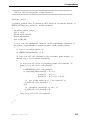
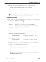
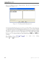
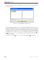
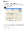
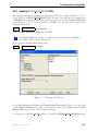
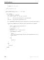
Example
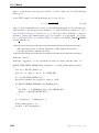
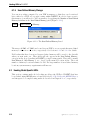
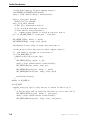
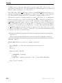
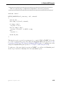
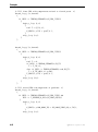
The following UDF, named reset udm, resets all user-defined memory (UDM) values
when a reset button on a user-defined GUI panel is clicked. The clicking of the button
is represented by 0, which is passed to the UDF by the FLUENT solver.
/*********************************************************
UDF called from a user-defined GUI panel to reset all
all user-defined memory locations
**********************************************************/
#include "udf.h"
DEFINE_EXECUTE_FROM_GUI(reset_udm, myudflib, mode)
{
Domain *domain = Get_Domain(1); /* Get domain pointer */
Thread *t;
cell_t c;
int i;
/* Return if mode is not zero */
if (mode != 0) return;
/* Return if no User-Defined Memory is defined in FLUENT */
if (n_udm == 0) return;
/* Loop over all cell threads in domain */
thread_loop_c(t, domain)
{
/* Loop over all cells */
begin_c_loop(c, t)
{
/* Set all UDMs to zero */
for (i = 0; i < n_udm; i++)
{
C_UDMI(c, t, i) = 0.0;
}
}
end_c_loop(c, t);
}
}
c Fluent Inc. September 11, 2006
2-13
DEFINE Macros
Hooking an Execute From GUI UDF to FLUENT
After the UDF that you have defined using DEFINE EXECUTE FROM GUI is compiled (Chapter 5: Compiling UDFs), the function will not need to be hooked to FLUENT through
any graphics panels. Instead, the function will be searched automatically by the FLUENT solver when the execution of the UDF is requested (i.e., when a call is made from
a user-defined Scheme program to execute a C function).
2-14
c Fluent Inc. September 11, 2006
2.2 General Purpose DEFINE Macros
2.2.6 DEFINE EXECUTE ON LOADING
Description
DEFINE EXECUTE ON LOADING is a general-purpose macro that can be used to specify a
function that executes as soon as a compiled UDF library is loaded in FLUENT. This is
useful when you want to initialize or setup UDF models when a UDF library is loaded.
(Alternatively, if you save your case file when a shared library is loaded, then the UDF
will execute whenever the case file is subsequently read.)
Compiled UDF libraries are loaded using either the Compiled UDFs or the UDF Library
Manager panel (see Section 5.5: Load and Unload Libraries Using the UDF Library Manager
Panel). An EXECUTE ON LOADING UDF is the best place to reserve user-defined scalar
(UDS) and user-defined memory (UDM) for a particular library (Sections 3.2.8 and 3.2.9)
as well as set UDS and UDM names (Sections 3.2.8 and 3.2.9).
i
DEFINE EXECUTE ON LOADING UDFs can be executed only as compiled
UDFs.
Usage
DEFINE EXECUTE ON LOADING(name,libname)
Argument Type
symbol name
char *libname
Description
UDF name.
compiled UDF library name.
Function returns
void
There are two arguments to DEFINE EXECUTE ON LOADING: name and libname. You
supply a name for the UDF which will be used by FLUENT when reporting that the
EXECUTE ON LOADING UDF is being run. The libname is set by FLUENT to be the name
of the library (e.g., libudf) that you have specified (by entering a name or keeping the
default libudf). libname is passed so that you can use it in messages within your UDF.
c Fluent Inc. September 11, 2006
2-15
DEFINE Macros
Example 1
The following simple UDF named report version, prints a message on the console that
contains the version and release number of the library being loaded.
#include "udf.h"
static int version = 1;
static int release = 2;
DEFINE_EXECUTE_ON_LOADING(report_version, libname)
{
Message("\nLoading %s version %d.%d\n",libname,version,release);
}
Example 2
The following source code contains two UDFs. The first UDF is an EXECUTE ON LOADING
function that is used to reserve three UDMs (using Reserve User Memory Vars) for a
library and set unique names for the UDM locations (using Set User Memory Name). The
second UDF is an ON DEMAND function that is used to set the values of the UDM locations
after the solution has been initialized. The ON DEMAND UDF sets the initial values of the
UDM locations using udm offset, which is defined in the on-loading UDF. Note that
the on demand UDF must be executed after the solution is initialized to reset the initial
values for the UDMs. See Sections 3.2.9 and 3.2.9 for more information on reserving and
naming UDMs.
/**********************************************************************
udm_res1.c contains two UDFs: an execute on loading UDF that reserves
three UDMs for libudf and renames the UDMs to enhance postprocessing,
and an on-demand UDF that sets the initial value of the UDMs.
**********************************************************************/
#include "udf.h"
#define NUM_UDM 3
static int udm_offset = UDM_UNRESERVED;
DEFINE_EXECUTE_ON_LOADING(on_loading, libname)
{
if (udm_offset == UDM_UNRESERVED) udm_offset =
Reserve_User_Memory_Vars(NUM_UDM);
if (udm_offset == UDM_UNRESERVED)
2-16
c Fluent Inc. September 11, 2006
2.2 General Purpose DEFINE Macros
Message("\nYou need to define up to %d extra UDMs in GUI and
then reload current library %s\n", NUM_UDM, libname);
else
{
Message("%d UDMs have been reserved by the current
library %s\n",NUM_UDM, libname);
Set_User_Memory_Name(udm_offset,"lib1-UDM-0");
Set_User_Memory_Name(udm_offset+1,"lib1-UDM-1");
Set_User_Memory_Name(udm_offset+2,"lib1-UDM-2");
}
Message("\nUDM Offset for Current Loaded Library = %d",udm_offset);
}
DEFINE_ON_DEMAND(set_udms)
{
Domain *d;
Thread *ct;
cell_t c;
int i;
d=Get_Domain(1);
if(udm_offset != UDM_UNRESERVED)
{
Message("Setting UDMs\n");
for (i=0;i<NUM_UDM;i++)
{
thread_loop_c(ct,d)
{
begin_c_loop(c,ct)
{
C_UDMI(c,ct,udm_offset+i)=3.0+i/10.0;
}
end_c_loop(c,ct)
}
}
}
else
Message("UDMs have not yet been reserved for library 1\n");
}
c Fluent Inc. September 11, 2006
2-17
DEFINE Macros
Hooking an Execute On Loading UDF to FLUENT
After the UDF that you have defined using DEFINE EXECUTE ON LOADING is compiled
(Chapter 5: Compiling UDFs), the function will not need to be hooked to FLUENT
through any graphics panels. Instead, FLUENT searches the newly-loaded library for any
UDFs of the type EXECUTE ON LOADING, and will automatically execute them in the order
they appear in the library.
2-18
c Fluent Inc. September 11, 2006
2.2 General Purpose DEFINE Macros
2.2.7 DEFINE INIT
Description
DEFINE INIT is a general-purpose macro that you can use to specify a set of initial values
for your solution. DEFINE INIT accomplishes the same result as patching, but does it
in a different way, by means of a UDF. A DEFINE INIT function is executed once per
initialization and is called immediately after the default initialization is performed by the
solver. Since it is called after the flow field is initialized, it is typically used to set initial
values of flow quantities. For an overview of the FLUENT solution process which shows
when a DEFINE INIT UDF is called, refer to Figures 1.9.1, 1.9.2, and 1.9.3.
Usage
DEFINE INIT(name,d)
Argument Type
symbol name
Domain *d
Description
UDF name.
Pointer to the domain over which the initialization function is
to be applied. The domain argument provides access to all cell
and face threads in the mesh. For multiphase flows, the pointer
that is passed to the function by the solver is the mixture-level
domain.
Function returns
void
There are two arguments to DEFINE INIT: name and d. You supply name, the name of
the UDF. d is passed from the FLUENT solver to your UDF.
Example
The following UDF, named my init func, initializes flow field variables in a solution. It
is executed once, at the beginning of the solution process. The function can be executed
as an interpreted or compiled UDF in FLUENT.
/***********************************************************************
UDF for initializing flow field variables
************************************************************************/
#include "udf.h"
DEFINE_INIT(my_init_func,d)
c Fluent Inc. September 11, 2006
2-19
DEFINE Macros
{
cell_t c;
Thread *t;
real xc[ND_ND];
/* loop over all cell threads in the domain
thread_loop_c(t,d)
{
*/
/* loop over all cells */
begin_c_loop_all(c,t)
{
C_CENTROID(xc,c,t);
if (sqrt(ND_SUM(pow(xc[0] - 0.5,2.),
pow(xc[1] - 0.5,2.),
pow(xc[2] - 0.5,2.))) < 0.25)
C_T(c,t) = 400.;
else
C_T(c,t) = 300.;
}
end_c_loop_all(c,t)
}
}
The macro ND SUM(a,b,c) computes the sum of the first two arguments (2D) or all
three arguments (3D). It is useful for writing functions involving vector operations so
that the same function can be used for 2D and 3D. For a 2D case, the third argument
is ignored. See Chapter 3: Additional Macros for Writing UDFs for a description of
predefined macros such as C CENTROID) and ND SUM.
Hooking an Initialization UDF to FLUENT
After the UDF that you have defined using DEFINE INIT is interpreted (Chapter 4: Interpreting UDFs) or compiled (Chapter 5: Compiling UDFs), the name of the argument
that you supplied as the first DEFINE macro argument (e.g., my init func) will become
visible and selectable in the User-Defined Function Hooks panel in FLUENT. Note that you
can hook multiple init functions to your model. See Section 6.1.5: Hooking DEFINE INIT
UDFs for details.
2-20
c Fluent Inc. September 11, 2006
2.2 General Purpose DEFINE Macros
2.2.8 DEFINE ON DEMAND
Description
DEFINE ON DEMAND is a general-purpose macro that you can use to specify a UDF that
is executed “on demand” in FLUENT, rather than having FLUENT call it automatically
during the calculation. Your UDF will be executed immediately, once it is activated,
but it is not accessible while the solver is iterating. Note that the domain pointer d
is not explicitly passed as an argument to DEFINE ON DEMAND. Therefore, if you want
to use the domain variable in your on-demand function, you will need to first retrieve
it using the Get Domain utility provided by Fluent (shown in the example below). See
Section 3.2.6: Domain Pointer (Get Domain) for details on Get Domain.
Usage
DEFINE ON DEMAND(name)
Argument Type
symbol name
Description
UDF name.
Function returns
void
There is only one argument to DEFINE ON DEMAND: name. You supply name, the name of
the UDF.
Example
The following UDF, named on demand calc, computes and prints the minimum, maximum, and average temperatures for the current data field. It then computes a temperature function
f (T ) =
T − Tmin
Tmax − Tmin
and stores it in user-defined memory location 0 (which is allocated as described in Section 3.2.3: Cell Macros). Once you hook the on-demand UDF (as described in Section 6.1.6: Hooking DEFINE ON DEMAND UDFs), the field values for f (T ) will be available
in drop-down lists in post-processing panels in FLUENT. You can select this field by
choosing User Memory 0 in the User Defined Memory... category. If you write a data file
after executing the UDF, the user-defined memory field will be saved to the data file.
This source code can be interpreted or compiled in FLUENT.
c Fluent Inc. September 11, 2006
2-21
DEFINE Macros
/**********************************************************************
UDF to calculate temperature field function and store in
user-defined memory. Also print min, max, avg temperatures.
***********************************************************************/
#include "udf.h"
DEFINE_ON_DEMAND(on_demand_calc)
{
Domain *d; /* declare domain pointer since it is not passed as an
argument to the DEFINE macro */
real tavg = 0.;
real tmax = 0.;
real tmin = 0.;
real temp,volume,vol_tot;
Thread *t;
cell_t c;
d = Get_Domain(1);
/* Get the domain using Fluent utility */
/* Loop over all cell threads in the domain */
thread_loop_c(t,d)
{
/* Compute max, min, volume-averaged temperature */
/* Loop over all cells */
begin_c_loop(c,t)
{
volume = C_VOLUME(c,t);
temp = C_T(c,t);
/* get cell volume */
/* get cell temperature */
if (temp < tmin || tmin == 0.) tmin = temp;
if (temp > tmax || tmax == 0.) tmax = temp;
vol_tot += volume;
tavg += temp*volume;
}
end_c_loop(c,t)
tavg /= vol_tot;
printf("\n Tmin = %g
2-22
Tmax = %g
Tavg = %g\n",tmin,tmax,tavg);
c Fluent Inc. September 11, 2006
2.2 General Purpose DEFINE Macros
/* Compute temperature function and store in user-defined memory*/
/*(location index 0)
*/
begin_c_loop(c,t)
{
temp = C_T(c,t);
C_UDMI(c,t,0) = (temp-tmin)/(tmax-tmin);
}
end_c_loop(c,t)
}
}
Get Domain is a macro that retrieves the pointer to a domain. It is necessary to get
the domain pointer using this macro since it is not explicitly passed as an argument
to DEFINE ON DEMAND. The function, named on demand calc, does not take any explicit
arguments. Within the function body, the variables that are to be used by the function
are defined and initialized first. Following the variable declarations, a looping macro
is used to loop over each cell thread in the domain. Within that loop another loop
is used to loop over all the cells. Within the inner loop, the total volume and the
minimum, maximum, and volume-averaged temperature are computed. These computed
values are printed to the FLUENT console. Then a second loop over each cell is used
to compute the function f (T ) and store it in user-defined memory location 0. Refer to
Chapter 3: Additional Macros for Writing UDFs for a description of predefined macros
such as C T and begin c loop.
Hooking an On-Demand UDF to FLUENT
After the UDF that you have defined using DEFINE ON DEMAND is interpreted (Chapter 4: Interpreting UDFs) or compiled (Chapter 5: Compiling UDFs), the name of the
argument that you supplied as the first DEFINE macro argument (e.g., on demand calc)
will become visible and selectable in the Execute On Demand panel in FLUENT. See
Section 6.1.6: Hooking DEFINE ON DEMAND UDFs for details.
c Fluent Inc. September 11, 2006
2-23
DEFINE Macros
2.2.9 DEFINE RW FILE
Description
DEFINE RW FILE is a general-purpose macro that you can use to specify customized information that is to be written to a case or data file, or read from a case or data file. You
can save and restore custom variables of any data type (e.g., integer, real, CXBoolean,
structure) using DEFINE RW FILE. It is often useful to save dynamic information (e.g.,
number of occurrences in conditional sampling) while your solution is being calculated,
which is another use of this function. Note that the read order and the write order must
be the same when you use this function.
Usage
DEFINE RW FILE(name,fp)
Argument Type
symbol name
FILE *fp
Description
UDF name.
Pointer to the file you are reading or writing.
Function returns
void
There are two arguments to DEFINE RW FILE: name and fp. You supply name, the name
of the UDF. fp is passed from the solver to the UDF.
i
DEFINE RW FILE cannot be used in UDFs that are executed on Windows
systems.
Example
The following C source code listing contains examples of functions that write information
to a data file and read it back. These functions are concatenated into a single source file
that can be interpreted or compiled in FLUENT.
/***********************************************************************
UDFs that increment a variable, write it to a data file
and read it back in
************************************************************************/
#include "udf.h"
int kount = 0;
2-24
/* define global variable kount */
c Fluent Inc. September 11, 2006
2.2 General Purpose DEFINE Macros
DEFINE_ADJUST(demo_calc,d)
{
kount++;
printf("kount = %d\n",kount);
}
DEFINE_RW_FILE(writer,fp)
{
printf("Writing UDF data to data file...\n");
fprintf(fp,"%d",kount); /* write out kount to data file */
}
DEFINE_RW_FILE(reader,fp)
{
printf("Reading UDF data from data file...\n");
fscanf(fp,"%d",&kount); /* read kount from data file */
}
At the top of the listing, the integer kount is defined and initialized to zero. The
first function (demo calc) is an ADJUST function that increments the value of kount
at each iteration, since the ADJUST function is called once per iteration. (See Section 2.2.1: DEFINE ADJUST for more information about ADJUST functions.) The second
function (writer) instructs FLUENT to write the current value of kount to the data file,
when the data file is saved. The third function (reader) instructs FLUENT to read the
value of kount from the data file, when the data file is read.
The functions work together as follows. If you run your calculation for, say, 10 iterations
(kount has been incremented to a value of 10) and save the data file, then the current
value of kount (10) will be written to your data file. If you read the data back into
FLUENT and continue the calculation, kount will start at a value of 10 and will be
incremented at each iteration. Note that you can save as many static variables as you
want, but you must be sure to read them in the same order in which they are written.
Hooking a Read/Write Case or Data File UDF to FLUENT
After the UDF that you have defined using DEFINE RW FILE is interpreted (Chapter 4: Interpreting UDFs) or compiled (Chapter 5: Compiling UDFs), the name of the argument that you supplied as the first DEFINE macro argument (e.g., writer) will become
visible and selectable in the User-Defined Function Hooks panel in FLUENT. Note that
you can hook multiple read/write functions to your model. See Section 6.1.7: Hooking
DEFINE RW FILE UDFs for details.
c Fluent Inc. September 11, 2006
2-25
DEFINE Macros
2.3
Model-Specific DEFINE Macros
The DEFINE macros presented in this section are used to set parameters for a particular
model in FLUENT. Table 2.3 provides a quick reference guide to the DEFINE macros, the
functions they are used to define, and the panels where they are activated in FLUENT.
Definitions of each DEFINE macro are listed in udf.h. For your convenience, they are
listed in Appendix B.
• Section 2.3.1: DEFINE CHEM STEP
• Section 2.3.2: DEFINE CPHI
• Section 2.3.3: DEFINE DIFFUSIVITY
• Section 2.3.4: DEFINE DOM DIFFUSE REFLECTIVITY
• Section 2.3.5: DEFINE DOM SOURCE
• Section 2.3.6: DEFINE DOM SPECULAR REFLECTIVITY
• Section 2.3.7: DEFINE GRAY BAND ABS COEFF
• Section 2.3.8: DEFINE HEAT FLUX
• Section 2.3.9: DEFINE NET REACTION RATE
• Section 2.3.10: DEFINE NOX RATE
• Section 2.3.11: DEFINE PR RATE
• Section 2.3.12: DEFINE PRANDTL UDFs
• Section 2.3.13: DEFINE PROFILE
• Section 2.3.14: DEFINE PROPERTY UDFs
• Section 2.3.15: DEFINE SCAT PHASE FUNC
• Section 2.3.16: DEFINE SOLAR INTENSITY
• Section 2.3.17: DEFINE SOURCE
• Section 2.3.18: DEFINE SOX RATE
• Section 2.3.19: DEFINE SR RATE
• Section 2.3.20: DEFINE TURB PREMIX SOURCE
• Section 2.3.21: DEFINE TURBULENT VISCOSITY
• Section 2.3.22: DEFINE VR RATE
• Section 2.3.23: DEFINE WALL FUNCTIONS
2-26
c Fluent Inc. September 11, 2006
2.3 Model-Specific DEFINE Macros
Table 2.3.1: Quick Reference Guide for Model-Specific DEFINE Functions
Function
mixing constant
homogeneous net mass
reaction rate for all
species, integrated over
a time step
species mass or UDS
diffusivity
diffusive reflectivity for
discrete ordinates (DO) model
source for DO model
specular reflectivity for
DO model
gray band absorption
coefficient for DO model
wall heat flux
homogeneous net mass
reaction rate for all species
NOx formation rates for
Thermal NO, Prompt NO,
Fuel NO, and N2O
Pathways
particle surface reaction rate
Prandtl numbers
species mass fraction
c Fluent Inc. September 11, 2006
DEFINE Macro
DEFINE CPHI
DEFINE CHEM STEP
Panel Activated In
User-Defined Function Hooks
User-Defined Function Hooks
DEFINE DIFFUSIVITY Materials
DEFINE DOM DIFFUSE
REFLECTIVITY
DEFINE DOM SOURCE
DEFINE DOM SPECULAR
REFLECTIVITY
DEFINE GRAY BAND
ABS COEFF
DEFINE HEAT FLUX
DEFINE NET
REACTION RATE
DEFINE NOX RATE
DEFINE PR RATE
DEFINE PRANDTL
DEFINE PROFILE
User-Defined Function Hooks
User-Defined Function Hooks
User-Defined Function Hooks
Materials
User-Defined Function Hooks
User-Defined Function Hooks
NOx Model
User-Defined Function Hooks
Viscous Model
boundary condition
(e.g., Velocity Inlet)
2-27
DEFINE Macros
Table 2.3.2: Quick Reference Guide for Model-Specific DEFINE Functions
Continued
2-28
Function
velocity at a boundary
DEFINE Macro
DEFINE PROFILE
pressure at a boundary
temperature at a boundary
mass flux at a boundary
target mass flow rate for
pressure outlet
turbulence kinetic energy
turbulence dissipation rate
specific dissipation rate
porosity
viscous resistance
inertial resistance
porous resistance direction
vector
user-defined scalar boundary
value
internal emissivity
wall thermal conditions
(heat flux, heat generation
rate, temperature, heat transfer
coefficient, external emissivity,
external radiation and free
stream temperature)
wall radiation
(internal emissivity,
irradiation)
wall momentum
(shear stress x,y,z components
swirl component, moving wall
velocity components, roughness
height, roughness constant)
wall species mass fractions
wall user-defined scalar
boundary
value
wall discrete phase boundary
value
wall functions
DEFINE
DEFINE
DEFINE
DEFINE
PROFILE
PROFILE
PROFILE
PROFILE
Panel Activated In
boundary condition
(e.g., Velocity Inlet)
boundary condition
boundary condition
boundary condition
Pressure Outlet
DEFINE
DEFINE
DEFINE
DEFINE
DEFINE
DEFINE
DEFINE
PROFILE
PROFILE
PROFILE
PROFILE
PROFILE
PROFILE
PROFILE
boundary
boundary
boundary
boundary
boundary
boundary
boundary
condition
condition
condition
condition
condition
condition
condition
DEFINE PROFILE
boundary condition
DEFINE PROFILE
DEFINE PROFILE
boundary condition
boundary condition
DEFINE PROFILE
boundary condition
DEFINE PROFILE
boundary condition
DEFINE PROFILE
DEFINE PROFILE
boundary condition
boundary condition
DEFINE PROFILE
boundary condition
DEFINE WALL FUNCTIONS Wall
c Fluent Inc. September 11, 2006
2.3 Model-Specific DEFINE Macros
Table 2.3.3: Quick Reference Guide for Model-Specific DEFINE Functions Continued
Function
density (as function of
temperature)
density (as function of
pressure for compressible
liquids)
viscosity
mass diffusivity
thermal conductivity
thermal diffusion coefficient
absorption coefficient
scattering coefficient
laminar flow speed
rate of strain
speed of sound function
user-defined mixing law for
mixture materials (density
viscosity, thermal conductivity)
scattering phase function
solar intensity
mass source
momentum source
energy source
turbulence kinetic energy
source
turbulence dissipation rate
source
species mass fraction source
user-defined scalar source
P1 radiation model source
surface reaction rate
SOx formation rate
turbulent premixed source
turbulent viscosity
UDS flux function
UDS unsteady function
wall function
volume reaction rate
c Fluent Inc. September 11, 2006
DEFINE Macro
DEFINE PROPERTY
Panel Activated In
Materials
DEFINE PROPERTY
Materials
DEFINE
DEFINE
DEFINE
DEFINE
DEFINE
DEFINE
DEFINE
DEFINE
DEFINE
DEFINE
PROPERTY
PROPERTY
PROPERTY
PROPERTY
PROPERTY
PROPERTY
PROPERTY
PROPERTY
PROPERTY
PROPERTY
Materials
Materials
Materials
Materials
Materials
Materials
Materials
Materials
Materials
Materials
DEFINE
DEFINE
DEFINE
DEFINE
DEFINE
DEFINE
SCAT PHASE FUNC
SOLAR INTENSITY
SOURCE
SOURCE
SOURCE
SOURCE
Materials
Radiation Model
boundary condition
boundary condition
boundary condition
boundary condition
DEFINE SOURCE
boundary condition
DEFINE SOURCE
DEFINE SOURCE
DEFINE SOURCE
DEFINE SR RATE
DEFINE SOX RATE
DEFINE TURB PREMIX
SOURCE
DEFINE TURBULENT
VISCOSITY
DEFINE UDS FLUX
DEFINE UDS UNSTEADY
DEFINE WALL FUNCTIONS
DEFINE VR RATE
boundary condition
boundary condition
boundary condition
User-Defined Function
SOx Model
User-Defined Function
Hooks
Viscous Model
User-Defined Scalars
User-Defined Scalars
boundary condition
User-Defined Function
Hooks
2-29
DEFINE Macros
Table 2.3.4: Quick Reference Guide for Model-Specific DEFINE Functions
MULTIPHASE ONLY
Function
volume fraction
(all multiphase models)
contact angle (VOF)
heat transfer coefficient
(Eulerian)
surface tension coefficient
(VOF)
cavitation surface tension
coefficient (Mixture)
cavitation vaporization
pressure (Mixture)
particle or droplet diameter
(Mixture)
temperature source
(Eulerian, Mixture)
diameter (Eulerian, Mixture)
solids pressure
(Eulerian, Mixture)
radial distribution
(Eulerian, Mixture)
elasticity modulus
(Eulerian, Mixture)
viscosity (Eulerian, Mixture)
temperature
(Eulerian, Mixture)
bulk viscosity (Eulerian)
frictional viscosity (Eulerian)
frictional pressure (Eulerian)
frictional modulus (Eulerian)
granular viscosity (Eulerian)
granular bulk viscosity
(Eulerian)
granular conductivity (Eulerian)
2-30
DEFINE Macro
DEFINE PROFILE
Panel Activated In
boundary condition
DEFINE PROFILE
DEFINE PROPERTY
Wall boundary condition
Phase Interaction
DEFINE PROPERTY
Phase Interaction
DEFINE PROPERTY
Phase Interaction
DEFINE PROPERTY
Phase Interaction
DEFINE PROPERTY
Materials
DEFINE SOURCE
boundary condition
DEFINE PROPERTY
DEFINE PROPERTY
Secondary Phase
Secondary Phase
DEFINE PROPERTY
Secondary Phase
DEFINE PROPERTY
Secondary Phase
DEFINE PROPERTY
DEFINE PROPERTY
Secondary Phase
Secondary Phase
DEFINE
DEFINE
DEFINE
DEFINE
DEFINE
DEFINE
Secondary
Secondary
Secondary
Secondary
Secondary
Secondary
PROPERTY
PROPERTY
PROPERTY
PROPERTY
PROPERTY
PROPERTY
DEFINE PROPERTY
Phase
Phase
Phase
Phase
Phase
Phase
Secondary Phase
c Fluent Inc. September 11, 2006
2.3 Model-Specific DEFINE Macros
2.3.1 DEFINE CHEM STEP
Description
You can use DEFINE CHEM STEP to compute the homogeneous net mass reaction rate of
all species integrated over a time step:
Yi∆t
=
Yi0
+
Z
0
∆t
dYi
dt
dt
(2.3-1)
where Yi0 is the initial mass fraction of species i, t is time, ∆t is the given time step,
i
and dY
is the net mass reaction rate. Yi∆t is ith species mass fraction at the end of the
dt
integration.
DEFINE CHEM STEP UDFs are used for the EDC and PDF Transport models.
Usage
DEFINE CHEM STEP(name,c,t,p,num p,n spe,dt,pres,
temp,yk)
Argument Type
symbol name
cell t c
Thread *t
Particle *p
int num p
int n spec
double *dt
double *pres
double *temp
double *yk
Description
UDF name.
Cell index of current particle.
Pointer to cell thread for particle.
Pointer to particle data structure that contains
data related to the particle being tracked.
Not Used.
Number of volumetric species.
Time step.
Pointer to pressure.
Pointer to temperature.
Pointer to array of initial species mass fractions.
Function returns
void
There are nine arguments to DEFINE CHEM STEP: name, c, p ,num p, n spe, dt, pres, temp,
and yk. You supply name, the name of the UDF. c, p, n spe, dt, pres, temp, and yk are
variables that are passed by the FLUENT solver to your UDF. num p is not used by the
function and can be ignored. The output of the function is the array of mass fractions
yk after the integration step. The initial mass fractions in array yk are overwritten.
c Fluent Inc. September 11, 2006
2-31
DEFINE Macros
Example
The following UDF, named user chem step, assumes that the net volumetric reaction
rate is the expression,
dYk
= 1/Nspe − Yk
dt
(2.3-2)
where Nspe is the number of species.
An analytic solution exists for the integral of this ODE as,
Yk∆t = (Yk0 − 1/Nspe )exp(−∆t) + 1/Nspe
(2.3-3)
/***************************************************
Example UDF that demonstrates DEFINE_CHEM_STEP
***************************************************/
#include "udf.h"
DEFINE_CHEM_STEP(user_chem_step,cell,thread,particle,nump,nspe,dt,pres,temp,yk)
{
int i;
double c = 1./(double)nspe;
double decay = exp(-(*dt));
for(i=0;i<n_spe;i++)
yk[i] = (yk[i]-c)*decay + c;
}
Hooking a Chemistry Step UDF to FLUENT
After the UDF that you have defined using DEFINE CHEM STEP is interpreted (Chapter 4: Interpreting UDFs) or compiled (Chapter 5: Compiling UDFs), the name of the
argument that you supplied as the first DEFINE macro argument (e.g., user chem step)
will become visible and selectable in the User-Defined Function Hooks panel in FLUENT.
See Section 6.2.1: Hooking DEFINE CHEM STEP UDFs for details.
2-32
c Fluent Inc. September 11, 2006
2.3 Model-Specific DEFINE Macros
2.3.2 DEFINE CPHI
Description
You can use DEFINE CPHI to set the value of the mixing constant Cφ (see Equation 18.2-6
and Equation 18.2-8 in the the User’s Guide for details.). It is useful for modeling flows
where Cφ departs substantially from its default value of 2, which occurs at low Reynolds
and/or high Schmidt numbers.
Usage
DEFINE CPHI(name,c,t)
Argument Type
symbol name
cell t c
Thread *t
Description
UDF name.
Cell index.
Pointer to cell thread.
Function returns
real
There are three arguments to DEFINE CPHI: name, c, and t. You supply name, the name
of the UDF. c and t are passed by the FLUENT solver to your UDF. Your UDF will need
to compute the real value of the mixing constant (Cφ ) and return it to the solver.
Hooking a Mixing Constant UDF to FLUENT
After the UDF that you have defined using DEFINE CPHI is interpreted (Chapter 4: Interpreting UDFs) or compiled (Chapter 5: Compiling UDFs), the name of the argument
that you supplied as the first DEFINE macro argument will become visible and selectable
in the Users Defined Function Hooks panel in FLUENT whenever the Composition PDF
Transport model is enabled. See Section 6.2.2: Hooking DEFINE CPHI UDFs for details.
c Fluent Inc. September 11, 2006
2-33
DEFINE Macros
2.3.3 DEFINE DIFFUSIVITY
Description
You can use DEFINE DIFFUSIVITY to specify the diffusivity for the species transport
equations (e.g., mass diffusivity) or for user-defined scalar (UDS) transport equations.
See Section 8.6: User-Defined Scalar (UDS) Diffusivity in the User’s Guide for details
about UDS diffusivity.
Usage
DEFINE DIFFUSIVITY(name,c,t,i)
Argument Type
symbol name
cell t c
Thread *t
int i
Description
UDF name.
Cell index.
Pointer to cell thread on which the diffusivity function is to
be applied.
Index that identifies the species or user-defined scalar.
Function returns
real
There are four arguments to DEFINE DIFFUSIVITY: name, c, and t, and i. You supply
name, the name of the UDF. c, t, and i are variables that are passed by the FLUENT
solver to your UDF. Your UDF will need to compute the diffusivity only for a single cell
and return the real value to the solver.
Note that diffusivity UDFs are called by FLUENT from within a loop on cell threads.
Consequently, your UDF will not need to loop over cells in a thread since FLUENT is
doing it outside of the function call.
2-34
c Fluent Inc. September 11, 2006
2.3 Model-Specific DEFINE Macros
Example
The following UDF, named mean age diff, computes the diffusivity for the mean age of
air using a user-defined scalar. Note that the mean age of air calculations do not require
that energy, radiation, or species transport calculations have been performed. You will
need to set uds-0 = 0.0 at all inlets and outlets in your model. This function can be
executed as an interpreted or compiled UDF.
/**********************************************************************
UDF that computes diffusivity for mean age using a user-defined
scalar.
***********************************************************************/
#include "udf.h"
DEFINE_DIFFUSIVITY(mean_age_diff,c,t,i)
{
return C_R(c,t) * 2.88e-05 + C_MU_EFF(c,t) / 0.7;
}
Hooking a Diffusivity UDF to FLUENT
After the UDF that you have defined using DEFINE DIFFUSIVITY is interpreted (Chapter 4: Interpreting UDFs) or compiled (Chapter 5: Compiling UDFs), the name that you
specified in the DEFINE macro argument (e.g., mean age diff) will become visible and selectable in the Materials panel in FLUENT. See Section 6.2.3: Hooking DEFINE DIFFUSIVITY
UDFs for details.
c Fluent Inc. September 11, 2006
2-35
DEFINE Macros
2.3.4 DEFINE DOM DIFFUSE REFLECTIVITY
Description
You can use DEFINE DOM DIFFUSE REFLECTIVITY to modify the inter-facial reflectivity
computed by FLUENT at diffusely reflecting semi-transparent walls, based on the refractive index values. During execution, a DEFINE DOM DIFFUSE REFLECTIVITY function is
called by FLUENT for each semi-transparent wall and also for each band (in the case of
a non-gray Discrete Ordinates Model). Therefore the function can be used to modify
diffuse reflectivity and diffuse transmissivity values at the interface.
Usage
DEFINE DOM DIFFUSE REFLECTIVITY(name,t,nb,n a,n b,diff ref a,diff tran a,
diff ref b,diff tran b)
i
Note that all of the arguments to a DEFINE macro need to be placed on the
same line in your source code. Splitting the DEFINE statement onto several
lines will result in a compilation error.
Argument Type
symbol name
Thread *t
Description
UDF name.
Pointer to the thread on which the discrete ordinate
diffusivity function is to be applied.
int nb
Band number (needed for the non-gray Discrete
Ordinates Model).
real n a
Refractive index of medium a.
real n b
Refractive index of medium b.
real *diff ref a
Diffuse reflectivity at the interface facing medium a.
real *diff tran a Diffuse transmissivity at the interface facing medium a.
real *diff ref b
Diffuse reflectivity at the interface facing medium b.
real *diff tran b Diffuse transmissivity at the interface facing medium b.
Function returns
void
There are nine arguments to DEFINE DOM DIFFUSE REFLECTIVITY: name, t, nb, n a, n b,
diff ref a, diff tran a, diff ref b, and diff tran b. You supply name, the name of
the UDF. t, nb, n a, n b, diff ref a, diff tran a, diff ref b, and diff tran b are
variables that are passed by the FLUENT solver to your UDF.
2-36
c Fluent Inc. September 11, 2006
2.3 Model-Specific DEFINE Macros
Example
The following UDF, named user dom diff refl, modifies diffuse reflectivity and transmissivity values on both the sides of the interface separating medium a and b. The UDF
is called for all the semi-transparent walls and prints the value of the diffuse reflectivity
and transmissivity values for side a and b.
/* UDF to print the diffuse reflectivity and transmissivity
at semi-transparent walls*/
#include "udf.h"
DEFINE_DOM_DIFFUSE_REFLECTIVITY(user_dom_diff_refl,t,nband,n_a,n_b,
diff_ref_a,diff_tran_a,diff_ref_b,diff_tran_b)
{
printf("diff_ref_a=%f diff_tran_a=%f \n", *diff_ref_a, *diff_tran_a);
printf("diff_ref_b=%f diff_tran_b=%f \n", *diff_ref_b, *diff_tran_b);
}
Hooking a Discrete Ordinates Model (DOM) Diffuse Reflectivity UDF to
FLUENT
After the UDF that you have defined using DEFINE DOM DIFFUSE REFLECTIVITY is interpreted (Chapter 4: Interpreting UDFs) or compiled (Chapter 5: Compiling UDFs),
the name of the argument that you supplied as the first DEFINE macro argument (e.g.,
user dom diff refl) will become visible and selectable in the User-Defined Function
Hooks panel in FLUENT. See Section 6.2.4: Hooking DEFINE DOM DIFFUSE REFLECTIVITY
UDFs for details.
c Fluent Inc. September 11, 2006
2-37
DEFINE Macros
2.3.5 DEFINE DOM SOURCE
Description
You can use DEFINE DOM SOURCE to modify the emission term (first term on the right
hand side in Equation 13.3-37 or Equation 13.3-38 of the User’s Guide ) as well as the
scattering term (second term on the right hand side of either equation) in the radiative
transport equation for the Discrete Ordinates (DO) model.
Usage
DEFINE DOM SOURCE(name,c,t,ni,nb,emission,in scattering,abs coeff,scat coeff)
Argument Type
symbol name
cell t c
Thread *t
int ni
int nb
real
real
real
real
Description
UDF name.
Cell index.
Pointer to cell thread.
Direction represented by the solid angle.
Band number (needed for the non-gray Discrete Ordinates
Model).
*emission
Pointer to emission term in the radiative transport
equation (Equation 13.3-37 to go to the User’s Guide manual).
*in scattering Pointer to scattering term in the radiative transport
equation (Equation 13.3-38 to go to the User’s Guide manual).
*abs coeff
Pointer to absorption coefficient.
*scat coeff
Pointer to scattering coefficient.
Function returns
void
There are nine arguments to DEFINE DOM SOURCE: name, c, ni, nb, emission,
in scattering, abs coeff, and scat coeff. You supply name, the name of the UDF.
c, ni, nb, emission, in scattering, abs coeff, and scat coeff are variables that are
passed by the FLUENT solver to your UDF. DEFINE DOM SOURCE is called by FLUENT for
each cell.
2-38
c Fluent Inc. September 11, 2006
2.3 Model-Specific DEFINE Macros
Example
In the following UDF, named user dom source, the emission term present in the radiative
transport equation is modified. The UDF is called for all the cells and increases the
emission term by 5%.
/* UDF to alter the emission source term in the DO model */
#include "udf.h"
DEFINE_DOM_SOURCE(user_dom_source,c,t,ni,nb,emission,in_scattering,
abs_coeff,scat_coeff)
{
/* increased the emission by 5 %
*emission
*/
*= 1.05;
}
i
Note that all of the arguments to a DEFINE macro need to be placed on the
same line in your source code. Splitting the DEFINE statement onto several
lines will result in a compilation error.
Hooking a DOM Source UDF to FLUENT
After the UDF that you have defined using DEFINE DOM SOURCE is interpreted (Chapter 4: Interpreting UDFs) or compiled (Chapter 5: Compiling UDFs), the name of the
argument that you supplied as the first DEFINE macro argument (e.g., user dom source)
will become visible and selectable in the User-Defined Function Hooks panel in FLUENT.
Note that you can hook multiple discrete ordinate source term functions to your model.
See Section 6.2.5: Hooking DEFINE DOM SOURCE UDFs for details.
c Fluent Inc. September 11, 2006
2-39
DEFINE Macros
2.3.6 DEFINE DOM SPECULAR REFLECTIVITY
Description
You can use DEFINE DOM SPECULAR REFLECTIVITY to modify the inter-facial reflectivity
of specularly reflecting semi-transparent walls. You may wish to do this if the reflectivity
is dependent on other conditions that the standard boundary condition doesn’t allow
for. (See Section 13.3.6: Specular Semi-Transparent Walls in the User’s Guide for more
information.) During FLUENT execution, the same UDF is called for all the faces of the
semi-transparent wall, for each of the directions.
Usage
DEFINE DOM SPECULAR REFLECTIVITY(name,f,t,nband,n a,n b,ray direction,en,
internal reflection,specular reflectivity,specular transmissivity)
i
Note that all of the arguments to a DEFINE macro need to be placed on the
same line in your source code. Splitting the DEFINE statement onto several
lines will result in a compilation error.
Argument Type
symbol name
face t f
Thread *t
Description
UDF name.
Face index.
Pointer to face thread on which the specular
reflectivity function is to be applied.
int nband
Band number (needed for non-gray Discrete
Ordinates Model).
real n a
Refractive index of medium a.
real n b
Refractive index of medium b.
real ray direction
Direction vector (s) defined
in Equation 13.3-55 in the User’s Guide
real en
Interface normal vector (n) defined
in Equation 13.3-55 in the User’s Guide
int internal reflection
Variable used to flag the code that total
internal reflection has occurred.
real *specular reflectivity
Specular reflectivity for the given direction s.
real *specular transmissivity Specular transmissivity for the given direction s.
Function returns
void
2-40
c Fluent Inc. September 11, 2006
2.3 Model-Specific DEFINE Macros
There are eleven arguments to DEFINE DOM SPECULAR REFLECTIVITY: name, f, t, nband,
n a, n b, ray direction, en, internal reflection, specular reflectivity, and
specular transmissivity.
You supply name, the name of the UDF. f,
t, nband, n a, n b, ray direction, en, internal reflection, specular reflectivity,
and specular transmissivity are variables that are passed by the FLUENT solver to
your UDF.
Example
In the following UDF, named user dom spec refl, specular reflectivity and transmissivity values are altered for a given ray direction s at face f.
/*
UDF to alter the specular reflectivity and transmissivity, at
semi-transparent walls, along direction s at face f */
#include "udf.h"
DEFINE_DOM_SPECULAR_REFLECTIVITY(user_dom_spec_refl,f,t, nband,n_a,n_b,
ray_direction,en,internal_reflection,specular_reflectivity,
specular_transmissivity)
{
real angle, cos_theta;
real PI = 3.141592;
cos_theta = NV_DOT(ray_direction, en);
angle = acos(cos_theta);
if (angle >45
&& angle < 60)
{
*specular_reflectivity = 0.3;
*specular_transmissivity = 0.7;
}
}
Hooking a Discrete Ordinate Model (DOM) Specular Reflectivity UDF to
FLUENT
After the UDF that you have defined using DEFINE DOM SPECULAR REFLECTIVITY is interpreted (Chapter 4: Interpreting UDFs) or compiled (Chapter 5: Compiling UDFs),
the name of the argument that you supplied as the first DEFINE macro argument (e.g.,
user dom spec refl) will become visible and selectable in the User-Defined Function
Hooks panel in FLUENT. See Section 6.2.6: Hooking DEFINE DOM SPECULAR REFLECTIVITY
UDFs for details.
c Fluent Inc. September 11, 2006
2-41
DEFINE Macros
2.3.7 DEFINE GRAY BAND ABS COEFF
Description
You can use DEFINE GRAY BAND ABS COEFF to specify a UDF for the gray band absorption
coefficient as a function of temperature, that can be used with a non-gray discrete ordinate
model.
Usage
DEFINE GRAY BAND ABS COEFF(name,c,t,nb)
Argument Type
symbol name
cell t c
Thread *t
int nb
Description
UDF name.
Cell index.
Pointer to cell thread.
Band number associated with non-gray model.
Function returns
real
There are four arguments to DEFINE GRAY BAND ABS COEFF: name, c, t, and nb. You
supply name, the name of the UDF. The variables c, t, and nb are passed by the FLUENT
solver to your UDF. Your UDF will need to return the real value of the gray band
coefficient to the solver.
Example
The following UDF, named user gray band abs, specifies the gray-band absorption coefficient as a function of temperature that can be used for a non-gray Discrete Ordinate
model.
#include
"udf.h"
DEFINE_GRAY_BAND_ABS_COEFF(user_gray_band_abs,c,t,nb)
{
real abs_coeff = 0;
real T = C_T(c,t);
switch (nb)
{
case 0 :
case 1 :
2-42
abs_coeff = 1.3+0.001*T; break;
abs_coeff = 2.7 + 0.005*T; break;
c Fluent Inc. September 11, 2006
2.3 Model-Specific DEFINE Macros
}
return abs_coeff;
}
Hooking a Gray Band Coefficient UDF to FLUENT
After the UDF that you have defined using DEFINE GRAY BAND ABS COEFF is interpreted
(Chapter 4: Interpreting UDFs) or compiled (Chapter 5: Compiling UDFs), the name of
the argument that you supplied as the first DEFINE macro argument
(e.g., user gray band abs) will become visible and selectable in the Materials panel
for the Absorption Coefficient. See Section 6.2.7: Hooking DEFINE GRAY BAND ABS COEFF
UDFs for details.
c Fluent Inc. September 11, 2006
2-43
DEFINE Macros
2.3.8 DEFINE HEAT FLUX
Description
You can use DEFINE HEAT FLUX to modify the heat flux at a wall. Despite the name,
a DEFINE HEAT FLUX UDF is not the means to specify the actual heat flux entering a
domain from the outside. To specify this type of heat flux, you would simply use a
DEFINE PROFILE function in conjunction with a heat flux thermal boundary condition.
In contrast, a DEFINE HEAT FLUX UDF allows you to modify the way in which the dependence between the flux entering the domain and the wall and cell temperatures is
modeled.
i
This function allows you to modify the heat flux at walls adjacent to a
solid.Note, however, that for solids since only heat conduction is occurring,
any extra heat flux that you add in a heat flux UDF can have a detrimental
effect on the solution of the energy equation. These effects will likely show
up in conjugate heat transfer problems. To avoid this, you will need to
make sure that your heat flux UDF excludes the walls adjacent to solids,
or includes only the necessary walls adjacent to fluid zones.
Usage
DEFINE HEAT FLUX(name,f,t,c0,t0,cid,cir)
Argument Type
symbol name
face t f
Thread *t
cell t c0
Thread *t0
real cid[]
real cir[]
Description
UDF name.
Index that identifies a wall face.
Pointer to wall face thread on which heat flux function is
to be applied.
Cell index that identifies the cell next to the wall.
Pointer to the adjacent cell’s thread.
Array of fluid-side diffusive heat transfer
coefficients.
Array of radiative heat transfer coefficients.
Function returns
void
2-44
c Fluent Inc. September 11, 2006
2.3 Model-Specific DEFINE Macros
There are seven arguments to DEFINE HEAT FLUX: name, f, t, c0, t0, cid, and cir. You
supply name, the name of the UDF. f, t, c0, and t0 are variables that are passed by
the FLUENT solver to your UDF. Arrays cir[] and cid[] contain the linearizations of
the radiative and diffusive heat fluxes, respectively, computed by FLUENT based on the
activated models. These arrays allow you to modify the heat flux in any way that you
choose. FLUENT computes the heat flux at the wall using these arrays after the call to
DEFINE HEAT FLUX, so the total heat flux at the wall will be the currently computed heat
flux (based on the activated models) with any modifications as defined by your UDF.
The diffusive heat flux (qid) and radiative heat flux (qir) are computed by FLUENT
according to the following equations:
qid = cid[0] + cid[1]*C_T(c0,t0) - cid[2]*F_T(f,t) - cid[3]*pow(F_T(f,t),4)
qir = cir[0] + cir[1]*C_T(c0,t0) - cir[2]*F_T(f,t) - cir[3]*pow(F_T(f,t),4)
The sum of qid and qir defines the total heat flux from the fluid to the wall (this
direction being positive flux), and, from an energy balance at the wall, equals the heat
flux of the surroundings (exterior to the domain). Note that heat flux UDFs (defined
using DEFINE HEAT FLUX) are called by FLUENT from within a loop over wall faces.
i
In order for the solver to compute C T and F T, the values you supply to
cid[1] and cid[2] should never be zero.
Example
Section 8.2.5: Implementing FLUENT’s P-1 Radiation Model Using User-Defined Scalars
provides an example of the P-1 radiation model implementation through a user-defined
scalar. An example of the usage of the DEFINE HEAT FLUX macro is included in that
implementation.
Hooking a Heat Flux UDF to FLUENT
After the UDF that you have defined using DEFINE HEAT FLUX is interpreted (Chapter 4: Interpreting UDFs) or compiled (Chapter 5: Compiling UDFs), the name of the
argument that you supplied as the first DEFINE macro argument (e.g., heat flux) will
become visible and selectable in the User-Defined Function Hooks panel in FLUENT. See
Section 6.2.8: Hooking DEFINE HEAT FLUX UDFs for details.
c Fluent Inc. September 11, 2006
2-45
DEFINE Macros
2.3.9 DEFINE NET REACTION RATE
Description
You can use DEFINE NET REACTION RATE to compute the homogeneous net molar reaction
rates of all species. The net reaction rate of a species is the sum over all reactions of the
volumetric reaction rates:
Ri =
NR
X
R̂i,r
(2.3-4)
r=1
where Ri is the net reaction rate of species i and R̂i,r is the Arrhenius molar rate of
creation/destruction of species i in reaction r.
A DEFINE NET REACTION RATE UDF may be used for the Laminar finite-rate, EDC, and
PDF Transport models, as well as for the surface chemistry model. In contrast, the
volumetric UDF function DEFINE VR RATE and surface UDF function DEFINE SR RATE
return the molar rate per reaction (R̂r ).
Usage
DEFINE NET REACTION RATE(name,c,t,particle,pressure,temp,yi,rr,jac)
Argument Type
symbol name
cell t c
Thread *t
Particle *particle
double
double
double
double
double
*pressure
*temp
*yi
*rr
*jac
Description
UDF name.
Cell index of current particle.
Pointer to cell thread for particle.
Pointer to Particle data structure that contains
data related to the particle being tracked.
Pointer to pressure variable.
Pointer to temperature variable.
Pointer to array containing species mass fractions.
Pointer to array containing net mass reaction rates.
Pointer to array of Jacobians.
Function returns
void
There are nine arguments to DEFINE NET REACTION RATE: name, c, t, particle, pressure,
temp, yi, rr, and jac. You supply name, the name of the UDF. The variables c, t,
particle, pressure, temp, yi, rr, and jac are passed by the FLUENT solver to your
UDF and have SI units. The outputs of the function are the array of net molar reaction
rates, rr (with units kgmol/m3 − s), and the Jacobian array jac. The Jacobian is only
2-46
c Fluent Inc. September 11, 2006
2.3 Model-Specific DEFINE Macros
required for surface chemistry, and is the derivative of the surface net reaction rate with
respect to the species concentration.
DEFINE NET REACTION RATE is called for all fluid zones (volumetric reactions as well as
surface reactions in porous media) and for all wall thread zones whenever the Reaction
button is enabled in the Boundary Conditions panel and the UDF is hooked to FLUENT
in the User-Defined Function Hooks panel.
i
DEFINE NET REACTION RATE functions can be executed only as compiled
UDFs.
Example
The following UDF, named user net reaction rate, assumes that the net volumetric
reaction rate is the expression,
Rnet = 1/Nspe − Yi
(2.3-5)
where Nspe is the number of species.
/***********************************************************
Net Reaction Rate Example UDF
************************************************************/
#include "udf.h"
DEFINE_NET_REACTION_RATE(user_net_reaction_rate,c,t,particle,
pressure,temp,yi,rr,jac)
{
int i;
for(i=0;i<n_spe;i++)
rr[i] = 1./(real)n_spe - yi[i];
}
Hooking a Net Mass Reaction Rate UDF to FLUENT
After the UDF that you have defined using DEFINE NET REACTION RATE is interpreted
(Chapter 4: Interpreting UDFs) or compiled (Chapter 5: Compiling UDFs), the name of
the argument that you supplied as the first DEFINE macro argument
(e.g., user net reaction rate) will become visible and selectable for the Net Reaction
Rate function in the User-Defined Function Hooks panel in FLUENT. See Section 6.2.9: Hooking DEFINE NET REACTION RATE UDFs for details.
c Fluent Inc. September 11, 2006
2-47
DEFINE Macros
2.3.10
DEFINE NOX RATE
Description
You can use the DEFINE NOX RATE to specify a custom NOx rate for thermal NO, prompt
NO, fuel NO and N2O intermediate pathways that can either replace the internallycalculated NOx rate in the source term equation, or be added to the FLUENT rate. The
default functionality is to add user-defined rates to the FLUENT-calculated rates. If the
Replace with UDF Rate checkbox is checked for a given NOx formation pathway in the
NOx Model panel, then the FLUENT-calculated rate for that NOx pathway will not be
used and it will instead be replaced by the NOx rate you have defined in your UDF.
When you hook a NOx rate UDF to the graphical interface without checking the Replace
with UDF Rate box for a particular pathway, then the user NOx rate will be added to the
internally-calculated rate for the source term calculation.
i
Note that a single UDF is used to define the different rates for the four
NOx pathways: thermal NO, prompt NO, fuel NO and N2O intermediate
pathway. That is, a NOx rate UDF can contain up to four separate rate
functions that are concatenated in a single source file which you hook to
FLUENT.
Usage
DEFINE NOX RATE(name,c,t,Pollut,Pollut Par,NOx)
Argument Type
symbol name
cell t c
Thread *t
Description
UDF name.
Cell index.
Pointer to cell thread on which the NOx rate
is to be applied.
Pollut Cell *Pollut
Pointer to the data structure that contains
the common data at each cell
Pollut Parameter *Pollut Par Pointer to the data structure
that contains auxiliary data.
NOx Parameter *NOx
Pointer to the data structure that contains
data specific to the NOx model.
Function returns
void
2-48
c Fluent Inc. September 11, 2006
2.3 Model-Specific DEFINE Macros
There are six arguments to DEFINE NOX RATE: name, c, t, Pollut, Pollut Par, and NOx.
You will supply name, the name of the UDF. c, t, Pollut, Pollut Par, and NOx are
variables that are passed by the FLUENT solver to your function. A DEFINE NOX RATE
function does not output a value. The calculated NO rates (or other pollutant species
rates) are returned through the Pollut structure as the forward rate Pollut->fwdrate
and reverse rate Pollut->revrate, respectively.
i
The data contained within the NOx structure is specific only to the NOx
model. Alternatively, the Pollut structure contains data at each cell that
are useful for all pollutant species (e.g., forward and reverse rates, gas
phase temperature, density). The Pollut Par structure contains auxiliary data common to all pollutant species (e.g., equation solved, universal
gas constant, species molecular weights). Note that molecular weights extracted from the Pollut Par structure (i.e., Pollut Par->sp[IDX(i)].mw)
has units of kg/kg − mol. The reverse rate calculated by user must be divided by the respective species mass fraction in order to be consistent with
the FLUENT 6.3 implementation (prior versions of FLUENT used explicit
division by species mass fraction internally).
Example
The following compiled UDF, named user nox, exactly reproduces the default FLUENT
NOx rates for the prompt NO pathway. Note that this UDF will replace the FLUENT
rate only if you select the Replace with UDF option for the prompt NO pathway in the
NOx Model panel.
See Section 3.2.7: NOx Macros for details about NOx macros (e.g., POLLUT EQN, MOLECON,
ARRH) that are used in pollutant rate calculations in this UDF.
/********************************************************************
UDF example of User-Defined NOx Rate
For FLUENT Versions 6.3 or above
If used with the "Replace with UDF" radio buttons activated,
this UDF will exactly reproduce the default fluent NOx
rates for prompt NO pathway.
The flag "Pollut_Par->pollut_io_pdf == IN_PDF" should always
be used for rates other than that from char N, so that if
requested, the contributions will be pdf-integrated. Any
contribution from char must be included within a switch
statement of the form "Pollut_Par->pollut_io_pdf == OUT_PDF".
*
* Arguments:
c Fluent Inc. September 11, 2006
2-49
DEFINE Macros
*
*
*
*
*
*
*
*
*
*
*
*
*
*
char nox_func_name
cell_t c
Thread *t
- UDF name
- Cell index
- Pointer to cell thread on
which the NOx rate is to be
applied
Pollut_Cell *Pollut
- Pointer to the data structure
that contains common data at
each cell.
structure
Pollut_Parameter *Pollut_Par - Pointer to the data structure
that contains auxillary data.
NOx_Parameter *NOx
- Pointer to the data structure
that contains data specific
to the NOx model.
*********************************************************************/
#include "udf.h"
DEFINE_NOX_RATE(user_nox, c, t, Pollut, Pollut_Par, NOx)
{
Pollut->fluct.fwdrate = 0.0;
Pollut->fluct.revrate = 0.0;
switch (Pollut_Par->pollut_io_pdf) {
case IN_PDF:
/* Source terms other than those from char must be included here*/
if (POLLUT_EQN(Pollut_Par) == EQ_NO) {
/* Prompt NOx */
if (NOx->prompt_nox && NOx->prompt_udf_replace) {
int j;
real f,rf;
real xc_fuel=0.0;
Rate_Const K_PM = {6.4e6,
0.0, 36483.49436};
f = 4.75 + 0.0819*NOx->c_number
- 23.2*NOx->equiv_ratio + 32.0*pow(NOx->equiv_ratio,2.)
- 12.2*pow(NOx->equiv_ratio,3.);
for (j=FUEL; j<FUEL+NOx->nfspe; j++) {
2-50
c Fluent Inc. September 11, 2006
2.3 Model-Specific DEFINE Macros
xc_fuel += MOLECON(Pollut, j);
}
rf = ARRH(Pollut, K_PM);
rf *= pow((Pollut_Par->uni_R*Pollut->temp_m/Pollut->press),
(1.+Pollut->oxy_order));
rf *= pow(MOLECON(Pollut, O2), Pollut->oxy_order);
rf *= MOLECON(Pollut, N2)*xc_fuel;
Pollut->fluct.fwdrate += f*rf;
}
}
case OUT_PDF:
/* Char Contributions, that do not go into pdf loop must be
included here */
break;
default:
;
}
}
Hooking a NOx Rate UDF to FLUENT
After the UDF that you have defined using DEFINE NOX RATE is interpreted (Chapter 4: Interpreting UDFs) or compiled (Chapter 5: Compiling UDFs), the name of the
argument that you supplied as the first DEFINE macro argument (e.g., user nox) will become visible and selectable in the NOx Model panel in FLUENT.
See Section 6.2.10: Hooking DEFINE NOX RATE UDFs for details.
c Fluent Inc. September 11, 2006
2-51
DEFINE Macros
2.3.11
DEFINE PR RATE
Description
You can use DEFINE PR RATE to specify a custom particle surface reaction for the multiple
surface reactions particle model. During FLUENT execution, the same UDF is called
sequentially for all particle surface reactions, so DEFINE PR RATE can be used to define
custom reaction rates for a single reaction, or for multiple reactions. The volumetric
and wall surface reactions are not affected by the definition of this macro and will follow
the designated rates. Note that a DEFINE PR RATE UDF is not called with the coupled
solution option, so you will need to disable the Coupled Heat Mass Solution option in
the Discrete Phase Model panel when using it. The auxiliary function, zbrent pr rate,
which is provided below, can be used when there is no analytical solution for the overall
particle reaction rate.
Usage
DEFINE PR RATE(name,c,t,r,mw,ci,p,sf,dif index,cat index,rr)
Argument Type
symbol name
cell t c
Thread *t
Reaction *r
Description
UDF name.
Cell index of current particle.
Pointer to cell thread for particle.
Pointer to data structure that represents the current
reaction.
real *mw
Pointer to array containing gaseous and surface species
molecular weights
real *ci
Pointer to array containing gas partial pressures.
Tracked Particle *p Pointer to Tracked Particle data structure that contains
data related to the particle being tracked.
real *sf
Pointer to array containing mass fractions of the solid
species in the particle char mass at the current time step.
int dif index
Diffusion controlled species as defined in the Reactions panel
for the current reaction.
Catalyst species as defined in the Reactions panel
int cat index
for the current reaction.
real *rr
Pointer to array containing particle reaction rate (kg/s).
Function returns
void
2-52
c Fluent Inc. September 11, 2006
2.3 Model-Specific DEFINE Macros
There are eleven arguments to DEFINE PR RATE: name, c, t, r, mw, ci, p, sf, dif index,
cat index, and rr. You supply name, the name of the UDF. c, t, r, mw, ci, p, sf,
dif index, cat index, and rr are variables that are passed by the FLUENT solver to
your UDF. Your UDF will need to set the value referenced by the real pointer rr to the
particle reaction rate in kg/s.
Note that p is an argument to many particle-specific macros defined in Section 3.2.7: DPM
Macros and can be used to obtain information about particle properties. Also note that
the order in which the solid species mass fractions are stored in array sf is the same as
the order in which the species are defined in the Selected Solid Species list in the Materials
panel, which is opened from the Edit Species names option for the Mixture Material.
DEFINE PR RATE is called by FLUENT every time step during the particle tracking calculation. The auxiliary function zbrent pr rate is used when there is no analytical
solution for the overall particle reaction rate. It uses Brent’s method to find the root of
a function known to lie between x1 and x2. The root will be refined until its accuracy
has reached tolerance tol. This is demonstrated in Example 2.
Auxiliary function
zbrent pr rate (real (*func),(real,real [],int [],cxboolean [],char *,) real
ruser[],int iuser[],
cxboolean buser[],char *cuser,real x1 real x2,real tol,cxboolean *ifail)
Auxiliary function returns: real
Example 1
The following UDF, named user pr rate, specifies a particle reaction rate given by
Equation 14.3-9 of the User’s Guide , where the effectiveness factor ηr is defined as
ηr = 1 − x
where x is the fractional conversion of the particle char mass. In this case, the UDF will
be applied to all surface particle reactions defined in the FLUENT model.
c Fluent Inc. September 11, 2006
2-53
DEFINE Macros
/* UDF of specifying the surface reaction rate of a particle */
#include "udf.h"
#define A1
#define E1
0.002
7.9e7
DEFINE_PR_RATE(user_pr_rate,c,t,r,mw,pp,p,sf,dif_i,cat_i,rr)
{
/* Argument types
cell_t c
Thread *t
Reaction *r (reaction structure)
real *mw (species molecular weight)
real *pp (gas partial pressures)
Tracked_Particle *p (particle structure)
real *sf
(current mass fractions of solid species in
particle char mass)
int dif_i (index of diffusion controlled species)
int cat_i (index of catalyst species)
real *rr
(rate of reaction kg/s)
*/
real ash_mass =
P_INIT_MASS(p)*(1.-DPM_CHAR_FRACTION(p)-DPM_VOLATILE_FRACTION(p));
real one_minus_conv =
MAX(0.,(P_MASS(p) -ash_mass) / P_INIT_MASS(p)/ DPM_CHAR_FRACTION(p));
real rate = A1*exp(-E1/UNIVERSAL_GAS_CONSTANT/P_T(p));
*rr=-rate*P_DIAM(p)*P_DIAM(p)*M_PI*sf[0]*one_minus_conv;
}
2-54
c Fluent Inc. September 11, 2006
2.3 Model-Specific DEFINE Macros
Example 2
The following compiled UDF, named user rate, specifies a particle reaction rate given
by Equation 14.3-4 to Equation 14.3-7 in the User’s Guide . The reaction order on the
kinetic rate is 0.9 and the effectiveness factor ηr is defined as
ηr = 1 − x
where x is the fractional conversion of the particle char mass. In this case it is necessary
to obtain a numerical solution for the overall surface reaction rate.
This UDF is called only for reaction 2, which means that the default FLUENT solution
will be used for the rest of the particle surface reactions defined.
/* UDF of specifying the surface reaction rate of a particle,
using a numerical solution */
#include "udf.h"
#define
#define
#define
#define
#define
c1 5e-12
A1 0.002
E1 7.9e7
tolerance 1e-4
order 0.9
real reaction_rate(real rate, real ruser[], int iuser[], cxboolean buser[],
char *cuser)
{
return (ruser[2]*pow(MAX(0.,(ruser[0]-rate/ruser[1])),order) -rate);
}
DEFINE_PR_RATE(user_rate,c,t,r,mw,pp,p,sf,dif_i,cat_i,rr)
{
if (!strcmp(r->name, "reaction-2"))
{
cxboolean ifail=FALSE;
real ash_mass =
P_INIT_MASS(p)*(1.-DPM_CHAR_FRACTION(p)-DPM_VOLATILE_FRACTION(p));
real one_minus_conv =
MAX(0.,(P_MASS(p) -ash_mass) / P_INIT_MASS(p)/ DPM_CHAR_FRACTION(p));
c Fluent Inc. September 11, 2006
2-55
DEFINE Macros
real ruser[3];
int iuser[1];
cxboolean buser[1];
char cuser[30];
real ratemin, ratemax, root;
ruser[0] = pp[dif_i];
ruser[1] = MAX(1.E-15, (c1*pow(0.5*(P_T(p)+C_T(c,t)),0.75)/P_DIAM(p)));
ruser[2] = A1*exp(-E1/UNIVERSAL_GAS_CONSTANT/P_T(p));
strcpy(cuser, "reaction-2");
ratemin=0;
ratemax=ruser[1]*pp[dif_i];
/* arguments for auxiliary function zbrent_pr_rate */
root = zbrent_pr_rate(reaction_rate, ruser, iuser, buser, cuser,
ratemin, ratemax, tolerance, &ifail);
if (ifail) root=MAX(1.E-15,ruser[1]);
*rr=-root*P_DIAM(p)*P_DIAM(p)*M_PI*sf[0]*one_minus_conv;
Message("Fail status %d\n", ifail);
Message("Reaction rate for reaction %s : %g\n", cuser, *rr);
}
}
In this example, a real function named reaction rate is defined at the top of the UDF.
The arguments of reaction rate are real rate, and the pointer arrays real ruser[],
integer iuser[], cxboolean buser[], and char *cuser, which must be declared and
defined in the main body of the DEFINE PR RATE function.
Typically, if the particle surface reaction rate is described by
rate = f(ruser[],iuser[],rate)
then the real function (in this example reaction rate) should return
f(ruser[],iuser[],rate) - rate
2-56
c Fluent Inc. September 11, 2006
2.3 Model-Specific DEFINE Macros
The variables cxboolean buser[] and char *cuser can be used to control the flow of
the program in cases of complicated rate definitions.
ratemin and ratemax, hold the minimum and maximum possible values of the variable
rate, respectively. They define the search interval where the numerical algorithm will
search for the root of the equation, as defined in the function reaction rate. The value
of reaction rate rr will be refined until an accuracy specified by the value of tolerance
tol is reached.
The variable ifail will take the value TRUE if the root of the function has not been
found.
Hooking a Particle Reaction Rate UDF to FLUENT
After the UDF that you have defined using DEFINE PR RATE is interpreted (Chapter 4: Interpreting UDFs) or compiled (Chapter 5: Compiling UDFs), the name of the argument
that you supplied as the first DEFINE macro argument (e.g., user pr rate) will become
visible and selectable in the User-Defined Function Hooks panel in FLUENT. See Section 6.2.11: Hooking DEFINE PR RATE UDFs for details.
c Fluent Inc. September 11, 2006
2-57
DEFINE Macros
2.3.12
DEFINE PRANDTL UDFs
The following DEFINE macros can be used to specify Prandtl numbers in FLUENT, for
single-phase flows.
DEFINE PRANDTL D
Description
You can use DEFINE PRANDTL D to specify Prandtl numbers for turbulent dissipation ().
Usage
DEFINE PRANDTL D(name,c,t)
Argument Type
symbol name
cell t c
Thread *t
Description
UDF name.
Index of cell on which the Prandtl number function is
to be applied.
Pointer to cell thread.
Function returns
real
There are three arguments to DEFINE PRANDTL D: name, c, and t. You supply name, the
name of the UDF. c and t are variables that are passed by the FLUENT solver to your
UDF. Your UDF will need to return the real value for the turbulent dissipation Prandtl
number to the solver.
Example
An example of a Prandtl D UDF is provided below in the source listing for DEFINE PRANDTL K.
Hooking a Prandtl Number UDF to FLUENT
After the UDF that you have defined using DEFINE PRANDTL D is interpreted (Chapter 4: Interpreting UDFs) or compiled (Chapter 5: Compiling UDFs), the name of
the argument that you supplied as the first DEFINE macro argument (e.g., user pr d)
will become visible and selectable in the Viscous Model panel in FLUENT. See Section 6.2.12: Hooking DEFINE PRANDTL UDFs for details.
2-58
c Fluent Inc. September 11, 2006
2.3 Model-Specific DEFINE Macros
DEFINE PRANDTL K
Description
You can use DEFINE PRANDTL K to specify Prandtl numbers for turbulence kinetic energy
(k).
Usage
DEFINE PRANDTL K(name,c,t)
Argument Type
symbol name
cell t c
Thread *t
Description
UDF name.
Index that identifies the cell on which the Prandtl number
function is to be applied.
Pointer to cell thread.
Function returns
real
There are three arguments to DEFINE PRANDTL K: name, c, and t. You supply name, the
name of the UDF. c and t are variables that are passed by the FLUENT solver to your
UDF. Your UDF will need to return the real value for the kinetic energy Prandtl number
to the solver.
Example
The following UDF implements a high-Re version of the RNG model, using the k- option
that is activated in FLUENT.
Three steps are required:
1. Set Cmu, C1eps, and C2eps as in the RNG model.
2. Calculate Prandtl numbers for k and using the UDF.
3. Add the -r source term in the equation.
In the RNG model, diffusion in k and equations appears as
(µ + µt ) ∗ α
while in the standard k- model, it is given by
c Fluent Inc. September 11, 2006
2-59
DEFINE Macros
µ+
µt
Pr
For the new implementation, a UDF is needed to define a Prandtl number P r as
Pr =
µt
[(µ + µt ) ∗ α − µ]
in order to achieve the same implementation as the original RNG Model.
The following functions (which are concatenated into a single C source code file) demonstrate this usage. Note that the source code must be executed as a compiled UDF.
#include "udf.h"
DEFINE_PRANDTL_K(user_pr_k,c,t)
{
real pr_k, alpha;
real mu
= C_MU_L(c,t);
real mu_t = C_MU_T(c,t);
alpha = rng_alpha(1., mu + mu_t, mu);
pr_k = mu_t/((mu+mu_t)*alpha-mu);
return pr_k;
}
DEFINE_PRANDTL_D(user_pr_d,c,t)
{
real pr_d, alpha;
real mu
= C_MU_L(c,t);
real mu_t = C_MU_T(c,t);
alpha = rng_alpha(1., mu + mu_t, mu);
pr_d = mu_t/((mu+mu_t)*alpha-mu);
return pr_d;
}
DEFINE_SOURCE(eps_r_source,c,t,dS,eqn)
2-60
c Fluent Inc. September 11, 2006
2.3 Model-Specific DEFINE Macros
{
real
real
real
real
real
real
con, source;
mu
= C_MU_L(c,t);
mu_t = C_MU_T(c,t);
k
= C_K(c,t);
d
= C_D(c,t);
prod = C_PRODUCTION(c,t);
real
real
real
real
s = sqrt(prod/(mu+ mu_t) ) ;
eta
= s*k/d;
eta_0 = 4.38;
term = mu_t*s*s*s/(1.0 + 0.012*eta*eta*eta);
source = - term * (1. - eta/eta_0);
dS[eqn] = - term/d;
return source;
}
Hooking a Prandtl Number UDF to FLUENT
After the UDF that you have defined using DEFINE PRANDTL K is interpreted (Chapter 4: Interpreting UDFs) or compiled (Chapter 5: Compiling UDFs), the name of
the argument that you supplied as the first DEFINE macro argument (e.g., user pr k)
will become visible and selectable in the Viscous Model panel in FLUENT. See Section 6.2.12: Hooking DEFINE PRANDTL UDFs for details.
c Fluent Inc. September 11, 2006
2-61
DEFINE Macros
DEFINE PRANDTL O
Description
You can use DEFINE PRANDTL O to specify Prandtl numbers for specific dissipation (ω in
the k-ω model).
Usage
DEFINE PRANDTL O(name,c,t)
Argument Type
symbol name
cell t c
Thread *t
Description
UDF name.
Index that identifies the cell on which the Prandtl number
function is to be applied.
Pointer to cell thread.
Function returns
real
There are three arguments to DEFINE PRANDTL O: name, c, and t. You supply name, the
name of the UDF. c and t are variables that are passed by the FLUENT solver to your
UDF. Your UDF will need to return the real value for the specific dissipation Prandtl
number to the solver.
Example
/* Specifying a Constant Specific Dissipation Prandtl Number */
#include "udf.h"
DEFINE_PRANDTL_O(user_pr_o,c,t)
{
real pr_o;
pr_o = 2.;
return pr_o;
}
2-62
c Fluent Inc. September 11, 2006
2.3 Model-Specific DEFINE Macros
Hooking a Prandtl Number UDF to FLUENT
After the UDF that you have defined using DEFINE PRANDTL O is interpreted (Chapter 4: Interpreting UDFs) or compiled (Chapter 5: Compiling UDFs), the name of
the argument that you supplied as the first DEFINE macro argument (e.g., user pr o)
will become visible and selectable in the Viscous Model panel in FLUENT. See Section 6.2.12: Hooking DEFINE PRANDTL UDFs for details.
DEFINE PRANDTL T
Description
You can use DEFINE PRANDTL T to specify Prandtl numbers that appear in the temperature equation diffusion term.
Usage
DEFINE PRANDTL T(name,c,t)
Argument Type
symbol name
cell t c
Thread *t
Description
UDF name.
Index that identifies the cell on which the Prandtl number
function is to be applied.
Pointer to cell thread.
Function returns
real
There are three arguments to DEFINE PRANDTL T: name, c, and t. You supply name, the
name of the UDF. c and t are variables that are passed by the FLUENT solver to your
UDF. Your UDF will need to return the real value for the temperature Prandtl number
to the solver.
c Fluent Inc. September 11, 2006
2-63
DEFINE Macros
Example
/* Specifying a Constant Temperature Prandtl Number */
#include "udf.h"
DEFINE_PRANDTL_T(user_pr_t,c,t)
{
real pr_t;
pr_t = 0.85;
return pr_t;
}
Hooking a Prandtl Number UDF to FLUENT
After the UDF that you have defined using DEFINE PRANDTL T is interpreted (Chapter 4: Interpreting UDFs) or compiled (Chapter 5: Compiling UDFs), the name of
the argument that you supplied as the first DEFINE macro argument (e.g., user pr t)
will become visible and selectable in the Viscous Model panel in FLUENT. See Section 6.2.12: Hooking DEFINE PRANDTL UDFs for details.
DEFINE PRANDTL T WALL
Description
You can use DEFINE PRANDTL T WALL to specify Prandtl numbers for thermal wall functions.
Usage
DEFINE PRANDTL T WALL(name,c,t)
Argument Type
symbol name
cell t c
Thread *t
Description
UDF name.
Index that identifies the cell on which the Prandtl number
function is to be applied.
Pointer to cell thread.
Function returns
real
2-64
c Fluent Inc. September 11, 2006
2.3 Model-Specific DEFINE Macros
There are three arguments to DEFINE PRANDTL T WALL: name, c, and t. You supply name,
the name of the UDF. c and t are variables that are passed by the FLUENT solver to
your UDF. Your UDF will need to return the real value for the thermal wall function
Prandtl number to the solver.
Example
/*************************************************************
Specifying a constant thermal wall function Prandtl number
********************************************************* **/
#include "udf.h"
DEFINE_PRANDTL_T_WALL(user_pr_t_wall,c,t)
{
real pr_t_wall;
pr_t_wall = 0.85;
return pr_t_wall;
}
Hooking a Prandtl Number UDF to FLUENT
After the UDF that you have defined using DEFINE PRANDTL T WALL is interpreted (Chapter 4: Interpreting UDFs) or compiled (Chapter 5: Compiling UDFs), the name of the
argument that you supplied as the first DEFINE macro argument (e.g., user pr t wall)
will become visible and selectable in the Viscous Model panel in FLUENT. See Section 6.2.12: Hooking DEFINE PRANDTL UDFs for details.
c Fluent Inc. September 11, 2006
2-65
DEFINE Macros
2.3.13
DEFINE PROFILE
Description
You can use DEFINE PROFILE to define a custom boundary profile that varies as a function
of spatial coordinates or time. Some of the variables you can customize at a boundary
are:
• velocity, pressure, temperature, turbulence kinetic energy, turbulence dissipation
rate
• mass flux
• target mass flow rate as a function of physical flow time
• species mass fraction (species transport)
• volume fraction (multiphase models)
• wall thermal conditions (temperature, heat flux, heat generation rate, heat transfer
coefficients, and external emissivity, etc.)
• wall roughness conditions
• wall shear and stress conditions
• porosity
• porous resistance direction vector
• wall adhesion contact angle (VOF multiphase model)
Note that DEFINE PROFILE allows you to modify only a single value for wall heat flux.
Single values are used in the explicit source term which FLUENT does not linearize. If
you want to linearize your source term for wall heat flux and account for conductive and
radiative heat transfer separately, you will need to use DEFINE HEAT FLUX to specify your
UDF.
Some examples of boundary profile UDFs are provided below. For an overview of the
FLUENT solution process which shows when a DEFINE PROFILE UDF is called, refer to
Figures 1.9.1, 1.9.2, and 1.9.3.
2-66
c Fluent Inc. September 11, 2006
2.3 Model-Specific DEFINE Macros
Usage
DEFINE PROFILE(name,t,i)
Argument Type
symbol name
Thread *t
int i
Description
UDF name.
Pointer to thread on which boundary condition is to be
applied.
Index that identifies the variable that is to be defined.
i is set when you hook the UDF with a variable in a boundary
condition panel through the graphical user interface. This index
is subsequently passed to your UDF by the FLUENT solver
so that your function knows which variable to operate on.
Function returns
void
There are three arguments to DEFINE PROFILE: name, t, and i. You supply name, the
name of the UDF. t and i are variables that are passed by the FLUENT solver to your
UDF.
While DEFINE PROFILE is usually used to specify a profile condition on a boundary face
zone, it can also be used to specify, or fix, flow variables that are held constant during
computation in a cell zone. (Click Section 7.27: Fixing the Values of Variables to go to
the User’s Guide for more information on fixing values in a cell zone boundary condition.)
For these cases, the arguments of the macro will change accordingly.
Note that unlike source term and property UDFs, profile UDFs (defined using
DEFINE PROFILE) are not called by FLUENT from within a loop on threads in the boundary zone. The solver passes only the pointer to the thread associated with the boundary
zone to the DEFINE PROFILE macro. Your UDF will need to do the work of looping over
all of the faces in the thread, computing the face value for the boundary variable, and
then storing the value in memory. Fluent has provided you with a face looping macro to
loop over all faces in a thread (begin f loop...). See Chapter 3: Additional Macros for
Writing UDFs for details.
F PROFILE is typically used along with DEFINE PROFILE and is a predefined macro supplied by Fluent. F PROFILE stores a boundary condition in memory for a given face and
thread and is nested within the face loop as shown in the examples below. It is important
to note that the index i that is an argument to DEFINE PROFILE is the same argument to
F PROFILE. F PROFILE uses the thread pointer t, face identifier f, and index i to set the
appropriate boundary face value in memory. See Section 3.2.6: Set Boundary Condition
Value (F PROFILE) for a description of F PROFILE. Note that in the case of porosity profiles, you can also utilize C PROFILE to define those types of functions. See the example
c Fluent Inc. September 11, 2006
2-67
DEFINE Macros
UDFs provided below.
In multiphase cases a DEFINE PROFILE UDF may be called more than once (particularly
if the profile is used in a mixture domain thread). If this needs to be avoided, then add
the prefix MP to the UDF name. The function will then be called only once even if it is
used for more than one profile.
Example 1 - Pressure Profile
The following UDF, named pressure profile, generates a parabolic pressure profile
according to the equation
5
5
p(y) = 1.1 × 10 − 0.1 × 10
y
0.0745
2
Note that this UDF assumes that the grid is generated such that the origin is at the
geometric center of the boundary zone to which the UDF is to be applied. y is 0.0 at
the center of the inlet and extends to ±0.0745 at the top and bottom of the inlet. The
source code can be interpreted or compiled in FLUENT.
/***********************************************************************
UDF for specifying steady-state parabolic pressure profile boundary
profile for a turbine vane
************************************************************************/
#include "udf.h"
DEFINE_PROFILE(pressure_profile,t,i)
{
real x[ND_ND];
/* this will hold the position vector */
real y;
face_t f;
begin_f_loop(f,t)
{
F_CENTROID(x,f,t);
y = x[1];
F_PROFILE(f,t,i) = 1.1e5 - y*y/(.0745*.0745)*0.1e5;
}
end_f_loop(f,t)
}
The function named pressure profile has two arguments: t and i. t is a pointer to
the face’s thread, and i is an integer that is a numerical label for the variable being set
within each loop.
2-68
c Fluent Inc. September 11, 2006
2.3 Model-Specific DEFINE Macros
Within the function body variable f is declared as a face. A one-dimensional array x
and variable y are declared as real data types. Following the variable declarations, a
looping macro is used to loop over each face in the zone to create a profile, or an array
of data. Within each loop, F CENTROID returns the value of the face centroid (array x)
for the face with index f that is on the thread pointed to by t. The y coordinate stored
in x[1] is assigned to variable y, and is then used to calculate the pressure. This value
is then assigned to F PROFILE which uses the integer i (passed to it by the solver, based
on your selection of the UDF as the boundary condition for pressure in the Pressure Inlet
panel) to set the pressure face value in memory.
Example 2 - Velocity, Turbulent Kinetic Energy, and Turbulent Dissipation Rate
Profiles
In the following example, DEFINE PROFILE is used to generate profiles for the x velocity,
turbulent kinetic energy, and dissipation rate, respectively, for a 2D fully-developed duct
flow. Three separate UDFs named x velocity, k profile, and dissip profile are
defined. These functions are concatenated in a single C source file and can be interpreted
or compiled in FLUENT.
The 1/7th power law is used to specify the x velocity component:
vx = vx,free
1/7
y
δ
A fully-developed profile occurs when δ is one-half the duct height. In this example,
the mean x velocity is prescribed and the peak (free-stream) velocity is determined by
averaging across the channel.
The turbulent kinetic energy is assumed to vary linearly from a near-wall value of
u2
knw = q τ
Cµ
to a free-stream value of
kinf = 0.002u2free
The dissipation rate is given by
=
Cµ3/4 (k 3/2 )
`
where the mixing length ` is the minimum of κy and 0.085δ. (κ is the von Karman
constant = 0.41.)
c Fluent Inc. September 11, 2006
2-69
DEFINE Macros
The friction velocity and wall shear take the forms:
uτ =
q
τw =
f ρu2free
2
τw /ρ
The friction factor is estimated from the Blasius equation:
ufree δ
f = 0.045
ν
!−1/4
/**********************************************************************
Concatenated UDFs for fully-developed turbulent inlet profiles
***********************************************************************/
/*#include "udf.h"*/
#define
#define
#define
#define
#define
#define
#define
#define
/*
YMIN 0.0
YMAX 0.4064
UMEAN 1.0
B 1./7.
DELOVRH 0.5
VISC 1.7894e-05
CMU 0.09
VKC 0.41
profile for x-velocity
/* constants
*/
*/
DEFINE_PROFILE(x_velocity,t,i)
{
real y, del, h, x[ND_ND], ufree;
face_t f;
/* variable declarations */
h = YMAX - YMIN;
del = DELOVRH*h;
ufree = UMEAN*(B+1.);
begin_f_loop(f,t)
2-70
c Fluent Inc. September 11, 2006
2.3 Model-Specific DEFINE Macros
{
F_CENTROID(x,f,t);
y = x[1];
if (y <= del)
F_PROFILE(f,t,i) = ufree*pow(y/del,B);
else
F_PROFILE(f,t,i) = ufree*pow((h-y)/del,B);
}
end_f_loop(f,t)
}
/*
profile for kinetic energy
*/
DEFINE_PROFILE(k_profile,t,i)
{
real y, del, h, ufree, x[ND_ND];
real ff, utau, knw, kinf;
face_t f;
h = YMAX - YMIN;
del = DELOVRH*h;
ufree = UMEAN*(B+1.);
ff = 0.045/pow(ufree*del/VISC,0.25);
utau=sqrt(ff*pow(ufree,2.)/2.0);
knw=pow(utau,2.)/sqrt(CMU);
kinf=0.002*pow(ufree,2.);
begin_f_loop(f,t)
{
F_CENTROID(x,f,t);
y=x[1];
if (y <= del)
F_PROFILE(f,t,i)=knw+y/del*(kinf-knw);
else
F_PROFILE(f,t,i)=knw+(h-y)/del*(kinf-knw);
}
end_f_loop(f,t)
}
/* profile for dissipation rate
c Fluent Inc. September 11, 2006
*/
2-71
DEFINE Macros
DEFINE_PROFILE(dissip_profile,t,i)
{
real y, x[ND_ND], del, h, ufree;
real ff, utau, knw, kinf;
real mix, kay;
face_t f;
h = YMAX - YMIN;
del = DELOVRH*h;
ufree = UMEAN*(B+1.);
ff = 0.045/pow(ufree*del/VISC,0.25);
utau=sqrt(ff*pow(ufree,2.)/2.0);
knw=pow(utau,2.)/sqrt(CMU);
kinf=0.002*pow(ufree,2.);
begin_f_loop(f,t)
{
F_CENTROID(x,f,t);
y=x[1];
if (y <= del)
kay=knw+y/del*(kinf-knw);
else
kay=knw+(h-y)/del*(kinf-knw);
if (VKC*y < 0.085*del)
mix = VKC*y;
else
mix = 0.085*del;
F_PROFILE(f,t,i)=pow(CMU,0.75)*pow(kay,1.5)/mix;
}
end_f_loop(f,t)
}
2-72
c Fluent Inc. September 11, 2006
2.3 Model-Specific DEFINE Macros
Example 3 - Fixed Velocity UDF
In the following example DEFINE PROFILE is used to fix flow variables that are held constant during computation in a cell zone. Three separate UDFs named fixed u, fixed v,
and fixed ke are defined in a single C source file. They specify fixed velocities that
simulate the transient startup of an impeller in an impeller-driven mixing tank. The
physical impeller is simulated by fixing the velocities and turbulence quantities using the
fix option in FLUENT. Click Section 7.27: Fixing the Values of Variables to go to the
User’s Guide for more information on fixing variables.
/***********************************************************************
Concatenated UDFs for simulating an impeller using fixed velocity
************************************************************************/
#include "udf.h"
#define
#define
#define
#define
#define
#define
FLUID_ID 1
ua1 -7.1357e-2
ua2 54.304
ua3 -3.1345e3
ua4 4.5578e4
ua5 -1.9664e5
#define
#define
#define
#define
#define
va1
va2
va3
va4
va5
3.1131e-2
-10.313
9.5558e2
-2.0051e4
1.1856e5
#define
#define
#define
#define
#define
#define
ka1
ka2
ka3
ka4
ka5
ka6
2.2723e-2
6.7989
-424.18
9.4615e3
-7.7251e4
1.8410e5
#define
#define
#define
#define
#define
#define
da1
da2
da3
da4
da5
da6
-6.5819e-2
88.845
-5.3731e3
1.1643e5
-9.1202e5
1.9567e6
c Fluent Inc. September 11, 2006
2-73
DEFINE Macros
DEFINE_PROFILE(fixed_u,t,i)
{
cell_t c;
real x[ND_ND];
real r;
begin_c_loop(c,t)
{
/* centroid is defined to specify position dependent profiles */
C_CENTROID(x,c,t);
r =x[1];
F_PROFILE(c,t,i) =
ua1+(ua2*r)+(ua3*r*r)+(ua4*r*r*r)+(ua5*r*r*r*r);
}
end_c_loop(c,t)
}
DEFINE_PROFILE(fixed_v,t,i)
{
cell_t c;
real x[ND_ND];
real r;
begin_c_loop(c,t)
{
/* centroid is defined to specify position dependent profiles*/
C_CENTROID(x,c,t);
r =x[1];
F_PROFILE(c,t,i) =
va1+(va2*r)+(va3*r*r)+(va4*r*r*r)+(va5*r*r*r*r);
}
end_c_loop(c,t)
}
DEFINE_PROFILE(fixed_ke,t,i)
{
cell_t c;
real x[ND_ND];
2-74
c Fluent Inc. September 11, 2006
2.3 Model-Specific DEFINE Macros
real r;
begin_c_loop(c,t)
{
/* centroid is defined to specify position dependent profiles*/
C_CENTROID(x,c,t);
r =x[1];
F_PROFILE(c,t,i) =
ka1+(ka2*r)+(ka3*r*r)+(ka4*r*r*r)+(ka5*r*r*r*r)+(ka6*r*r*r*r*r);
}
end_c_loop(c,t)
}
Example 4 - Wall Heat Generation Rate Profile
The following UDF, named wallheatgenerate, generates a heat generation rate profile
for a planar conduction wall. Once interpreted or compiled, you can activate this UDF
in the Wall boundary condition panel in FLUENT.
/*
Wall Heat Generation Rate Profile UDF
*/
#include "udf.h"
DEFINE_PROFILE(wallheatgenerate,thread,i)
{
real source = 0.001;
face_t f;
begin_f_loop(f,thread)
F_PROFILE(f,thread,i) = source;
end_f_loop(f,thread)
}
Example 5 - Viscous Resistance Profile in a Porous Zone
You can either use F PROFILE or C PROFILE to define a viscous resistance profile in a
porous zone. Below are two sample UDFs that demonstrate the usage of F PROFILE
and C PROFILE, respectively. Note that porosity functions are hooked to FLUENT in the
Porous Zone tab in the appropriate Fluid boundary conditions panel.
The following UDF, named vis res, generates a viscous resistance profile in a porous
zone. Once interpreted or compiled and loaded, you can activate this UDF in the Fluid
boundary condition panel in FLUENT.
c Fluent Inc. September 11, 2006
2-75
DEFINE Macros
/*
Viscous Resistance Profile UDF in a Porous Zone
that utilizes F_PROFILE*/
#include "udf.h"
DEFINE_PROFILE(vis_res,t,i)
{
real x[ND_ND];
real a;
cell_t c;
begin_c_loop(c,t)
{
C_CENTROID(x,c,t);
if( x[1] < (x[0]-0.01) )
a = 1e9;
else
a = 1.0;
F_PROFILE(c,t,i) = a;
}
end_c_loop(c,t)
}
/*
Viscous Resistance Profile UDF in a Porous Zone that utilizes C_PROFILE*/
#include "udf.h"
DEFINE_PROFILE{porosity_function, t, nv}
{
cell_t c;
begin_c_loop(c,t)
C_PROFILE(c,t,nv) = USER INPUT ;
end_c_loop(c,t)
}
2-76
c Fluent Inc. September 11, 2006
2.3 Model-Specific DEFINE Macros
Example 6 - Porous Resistance Direction Vector
The following UDF contains profile functions for two porous resistance direction vectors
that utilize C PROFILE. These profiles can be hooked to corresponding direction vectors
under Porous Zone in the Fluid boundary condition panel.
/*
Porous Resistance Direction Vector Profile that utilizes C_PROFILE*/
#include "udf.h"
DEFINE_PROFILE{dir1, t, nv}
{
cell_t c;
begin_c_loop(c,t)
C_PROFILE(c,t,nv) = USER INPUT1
end_c_loop(c,t)
}
DEFINE_PROFILE{dir2, t, nv}
{
cell_t c;
begin_c_loop(c,t)
C_PROFILE(c,t,nv) = USER INPUT2
end_c_loop(c,t)
}
;
;
Example 7 -Target Mass Flow Rate UDF as a Function of Physical Flow Time
For some unsteady problems, it is desirable that the target mass flow rate be a function of
the physical flow time. This boundary condition can be applied using a DEFINE PROFILE
UDF. The following UDF, named tm pout2, adjusts the mass flow rate from 1.00kg/s
to 1.35kg/s when the physical time step is greater than 0.2 seconds. Once interpreted
or compiled, you can activate this UDF in the Pressure Outlet boundary condition panel
in FLUENT by selecting the Specify target mass-flow rate option, and then choosing the
UDF name from the corresponding drop-down list.
i
Note that the mass flow rate profile is a function of time and only one
constant value should be applied to all zone faces at a given time.
/* UDF for setting target mass flow rate in pressure-outlet
*/
/* at t<0.2 sec the target mass flow rate set to 1.00 kg/s
*/
/* when t>0.2 sec the target mass flow rate will change to 1.35 kg/s */
c Fluent Inc. September 11, 2006
2-77
DEFINE Macros
#include "udf.h"
DEFINE_PROFILE(tm_pout2, t, nv)
{
face_t f ;
real flow_time = RP_Get_Real("flow-time");
if (flow_time < 0.2 )
{
printf("Time
= %f sec. \n",flow_time);
printf("Targeted mass-flow rate set at 1.0 kg/s \n");
begin_f_loop(f,t)
{
F_PROFILE(f,t,nv) = 1.0 ;
}
end_f_loop(f,t)
}
else
{
printf("Time
= %f sec. \n",flow_time);
printf("Targeted mass-flow rate set at 1.35 kg/s \n") ;
begin_f_loop(f,t)
{
F_PROFILE(f,t,nv) = 1.35 ;
}
end_f_loop(f,t)
}
}
Hooking a Boundary Profile UDF to FLUENT
After the UDF that you have defined using DEFINE PROFILE is interpreted (Chapter 4: Interpreting UDFs) or compiled (Chapter 5: Compiling UDFs), the name of the argument
that you supplied as the first DEFINE macro argument (e.g., vis res) will become visible
and selectable in the appropriate boundary condition panel (e.g., the Velocity Inlet panel)
in FLUENT. See Section 6.2.13: Hooking DEFINE PROFILE UDFs for details.
2-78
c Fluent Inc. September 11, 2006
2.3 Model-Specific DEFINE Macros
2.3.14
DEFINE PROPERTY UDFs
Description
You can use DEFINE PROPERTY to specify a custom material property in FLUENT for
single-phase and multiphase flows. When you are writing a user-defined mixing law UDF
for a mixture material, you will need to use special utilities to access species material
properties. These are described below. If you want to define a custom mass diffusivity
property when modeling species transport, you must use DEFINE DIFFUSIVITY instead of
DEFINE PROPERTY. See Section 2.3.3: DEFINE DIFFUSIVITY for details on
DEFINE DIFFUSIVITY UDFs. For an overview of the FLUENT solution process which
shows when a DEFINE PROPERTY UDF is called, refer to Figures 1.9.1, 1.9.2, and 1.9.3.
Some of the properties you can customize using DEFINE PROPERTY are:
• density (as a function of temperature)
• viscosity
• thermal conductivity
• absorption and scattering coefficients
• laminar flow speed
• rate of strain
• user-defined mixing laws for density, viscosity, and thermal conductivity of mixture
materials
i
UDFs cannot be used to define specific heat properties; specific heat data
can be accessed only and not modified in FLUENT.
i
Note that when you specify a user-defined density function for a compressible liquid flow application, you must also include a speed of sound
function in your model. Compressible liquid density UDFs can be used
in the pressure-based solver and for single phase, multiphase mixture and
cavitation models, only. See the example below for details.
c Fluent Inc. September 11, 2006
2-79
DEFINE Macros
For Multiphase Flows
• surface tension coefficient (VOF model)
• cavitation parameters including surface tension coefficient and vaporization pressure (Mixture, cavitation models)
• heat transfer coefficient (Mixture model)
• particle or droplet diameter (Mixture model)
• speed of sound function (Mixture, cavitation models)
• density (as a function of pressure) for compressible liquid flows only (Mixture,
cavitation models)
• granular temperature and viscosity (Mixture, Eulerian models)
• granular bulk viscosity (Eulerian model)
• granular conductivity (Eulerian model)
• frictional pressure and viscosity (Eulerian model)
• frictional modulus (Eulerian model)
• elasticity modulus (Eulerian model)
• radial distribution (Eulerian model)
• solids pressure (Eulerian, Mixture models)
• diameter (Eulerian, Mixture models)
Usage
DEFINE PROPERTY(name,c,t)
Argument Type
symbol name
cell t c
Thread *t
Description
UDF name.
Cell index.
Pointer to cell thread on which the property function is to be
applied.
Function returns
real
2-80
c Fluent Inc. September 11, 2006
2.3 Model-Specific DEFINE Macros
There are three arguments to DEFINE PROPERTY: name, c, and t. You supply name, the
name of the UDF. c and t are variables that are passed by the FLUENT solver to your
UDF. Your UDF will need to compute the real property only for a single cell and return
it to the solver.
Note that like source term UDFs, property UDFs (defined using DEFINE PROPERTY) are
called by FLUENT from within a loop on cell threads. The solver passes all of the variables
needed to allow a DEFINE PROPERTY UDF to define a custom material, since properties
are assigned on a cell basis. Consequently, your UDF will not need to loop over cells in
a zone since FLUENT is already doing it.
Auxiliary Utilities
Some commonly-used auxiliary utilities for custom property UDFs are described below.
They are generic property,
MATERIAL PROPERTY, THREAD MATERIAL, and
mixture species loop.
generic property is a general purpose function that returns the real value for the given
property id for the given thread material. It is defined in prop.h and is used only for
species properties.
The following Property ID variables are available:
• PROP rho, density
• PROP mu, viscosity
• PROP ktc, thermal conductivity
generic property (name,c,t,prop,id,T)
Argument Type
symbol name
cell t c
Thread *t
Property *prop
Property ID id
real T
Description
Function name.
Cell index.
Pointer to cell thread on which property function is to be
applied.
Pointer to property array for the thread material that can be
obtained through the macro MATERIAL PROPERTY(m) See below.
Property ID of the required property you want to define a
custom mixing law for (e.g., PROP ktc for thermal conductivity).
See below for list of variables.
Temperature at which the property is to be evaluated (used only
if a polynomial method is specified).
Function returns
real
c Fluent Inc. September 11, 2006
2-81
DEFINE Macros
MATERIAL PROPERTY is defined in materials.h and returns a real pointer to the Property
array prop for the given material pointer m.
MATERIAL PROPERTY(m)
Argument Type
Material *m
Description
Material pointer.
Function returns
real
THREAD MATERIAL is defined in threads.h and returns real pointer m to the Material
that is associated with the given cell thread t.
i
Note that in previous versions of FLUENT, THREAD MATERIAL took two
arguments (t,i), but now only takes one (t).
THREAD MATERIAL(t)
Argument Type
Thread *t
Description
Pointer to cell thread.
Function returns
real
mixture species loop is defined in materials.h and loops over all of the species for
the given mixture material.
mixture species loop (m,sp,i)
Argument Type
Material *m
Material *sp
int i
Description
Material pointer.
Species pointer.
Species index.
Function returns
real
2-82
c Fluent Inc. September 11, 2006
2.3 Model-Specific DEFINE Macros
Example 1 - Temperature-dependent Viscosity Property
The following UDF, named cell viscosity, generates a variable viscosity profile to
simulate solidification. The function is called for every cell in the zone. The viscosity in
the warm (T > 288 K) fluid has a molecular value for the liquid (5.5 ×10⁻³ kg/m-s), while
the viscosity for the cooler region (T < 286 K) has a much larger value (1.0 kg/m-s). In
the intermediate temperature range (286 K ≤ T ≤ 288 K), the viscosity follows a linear
profile that extends between the two values given above:
µ = 143.2135 − 0.49725T
(2.3-6)
This model is based on the assumption that as the liquid cools and rapidly becomes more
viscous, its velocity will decrease, thereby simulating solidification. Here, no correction
is made for the energy field to include the latent heat of freezing. The source code can
be interpreted or compiled in FLUENT.
/*********************************************************************
UDF that simulates solidification by specifying a temperaturedependent viscosity property
**********************************************************************/
#include "udf.h"
DEFINE_PROPERTY(cell_viscosity,c,t)
{
real mu_lam;
real temp = C_T(c,t);
if (temp > 288.)
mu_lam = 5.5e-3;
else if (temp > 286.)
mu_lam = 143.2135 - 0.49725 * temp;
else
mu_lam = 1.;
return mu_lam;
}
The function cell viscosity is defined on a cell. Two real variables are introduced:
temp, the value of C T(c,t), and mu lam, the laminar viscosity computed by the function.
The value of the temperature is checked, and based upon the range into which it falls,
the appropriate value of mu lam is computed. At the end of the function the computed
value for the viscosity (mu lam) is returned to the solver.
c Fluent Inc. September 11, 2006
2-83
DEFINE Macros
Example 2 - User-defined Mixing Law for Thermal Conductivity
You can use DEFINE PROPERTY to define custom user-defined mixing laws for density,
viscosity, and conductivity of mixture materials. In order to access species material
properties your UDF will need to utilize auxiliary utilities that are described above.
The following UDF, named mass wtd k, is an example of a mass-fraction weighted conductivity function. The UDF utilizes the generic property function to obtain properties
of individual species. It also makes use of MATERIAL PROPERTY and THREAD MATERIAL.
/*********************************************************************
UDF that specifies a custom mass-fraction weighted conductivity
**********************************************************************/
#include "udf.h"
DEFINE_PROPERTY(mass_wtd_k,c,t)
{
real sum = 0.; int i;
Material *sp;
real ktc;
Property *prop;
mixture_species_loop(THREAD_MATERIAL(t),sp,i)
{
prop = (MATERIAL_PROPERTY(sp));
ktc = generic_property(c,t,prop,PROP_ktc,C_T(c,t));
sum += C_YI(c,t,i)*ktc;
}
return sum;
}
2-84
c Fluent Inc. September 11, 2006
2.3 Model-Specific DEFINE Macros
Example 3 - Surface Tension Coefficient UDF
DEFINE PROPERTY can also be used to define a surface tension coefficient UDF for the
multiphase VOF model. The following UDF specifies a surface tension coefficient as a
quadratic function of temperature. The source code can be interpreted or compiled in
FLUENT.
/***************************************************************
Surface Tension Coefficient UDF for the multiphase VOF Model
***************************************************************/
#include "udf.h"
DEFINE_PROPERTY(sfc,c,t)
{
real T = C_T(c,t);
return 1.35 - 0.004*T + 5.0e-6*T*T;
}
i
Note that surface tension UDFs for the VOF and Mixture multiphase models are both hooked to FLUENT in the Phase Interaction panel, but in different ways. For the VOF model, the function hook is located in the Surface
Tension tab in the panel. For the Mixture model, however, the function
hook is located in the Mass tab, and will become visible upon selecting the
Cavitation option.
Example 4 - Density Function for Compressible Liquids
Liquid density is not a constant but is instead a function of the pressure field. In order to
stabilize the pressure solution for compressible flows in FLUENT, an extra term related
to the speed of sound is needed in the pressure correction equation. Consequently, when
you want to define a custom density function for a compressible flow, your model must
also include a speed of sound function. Although you can direct FLUENT to calculate a
speed of sound function by choosing one of the available methods (e.g., piecewise-linear,
polynomial) in the Materials panel, as a general guideline you should define a speed of
sound function along with your density UDF using the formulation:
q ∂p
(
∂ρ
)
For simplicity, it is recommended that you concatenate the density and speed of sound
functions into a single UDF source file.
c Fluent Inc. September 11, 2006
2-85
DEFINE Macros
The following UDF source code example contains two concatenated functions: a density
function named superfluid density that is defined in terms of pressure and a custom
speed of sound function named sound speed.
/********************************************************************
Density and speed of sound UDFs for compressible liquid flows.
For use with pressure-based solver, for single phase, multiphase mixture
or cavitation models only.
Note that for density function, dp is the difference between a cell
absolute pressure and reference pressure.
*********************************************************************/
#include "udf.h"
#define BMODULUS 2.2e9
#define rho_ref 1000.0
#define p_ref 101325
DEFINE_PROPERTY(superfluid_density, c, t)
{
real rho;
real p, dp;
real p_operating;
p_operating = RP_Get_Real ("operating-pressure");
p = C_P(c,t) + p_operating;
dp = p-p_ref;
rho = rho_ref/(1.0-dp/BMODULUS);
return rho;
}
DEFINE_PROPERTY(sound_speed, c,t)
{
real a;
real p, dp,p_operating;
p_operating = RP_Get_Real ("operating-pressure");
p = C_P(c,t) + p_operating;
dp = p-p_ref;
a = (1.-dp/BMODULUS)*sqrt(BMODULUS/rho_ref);
2-86
c Fluent Inc. September 11, 2006
2.3 Model-Specific DEFINE Macros
return a;
}
Hooking a Property UDF to FLUENT
After the UDF that you have defined using DEFINE PROPERTY is interpreted (Chapter 4: Interpreting UDFs) or compiled (Chapter 5: Compiling UDFs), the name of the
argument that you supplied as the first DEFINE macro argument (e.g., sound speed) will
become visible and selectable in graphics panels in FLUENT.
See Section 6.2.14: Hooking DEFINE PROPERTY UDFs for details.
c Fluent Inc. September 11, 2006
2-87
DEFINE Macros
2.3.15
DEFINE SCAT PHASE FUNC
Description
You can use DEFINE SCAT PHASE FUNC to specify the radiation scattering phase function
for the Discrete Ordinates (DO) model. The function computes two values: the fraction
of radiation energy scattered from direction i to direction j, and the forward scattering
factor.
Usage
DEFINE SCAT PHASE FUNC(name,cosine,f)
Argument Type
symbol name
real cosine
real *f
Description
UDF name.
Cosine of the angle between directions i and j.
Pointer to the location in memory where the real forward
scattering factor is stored.
Function returns
real
There are three arguments to DEFINE SCAT PHASE FUNC: name, cosine, and f. You supply
name, the name of the UDF. cosine and f are variables that are passed by the FLUENT
solver to your UDF. Your UDF will need to compute the real fraction of radiation energy
scattered from direction i to direction j and return it to the solver. Note that the solver
computes and stores a scattering matrix for each material by calling this function for
each unique pair of discrete ordinates.
Example
In the following example, a number of UDFs are concatenated in a single C source file.
These UDFs implement backward and forward scattering phase functions that are cited
by Jendoubi et al. [1]. The source code can be interpreted or compiled in FLUENT.
/*******************************************************************
UDFs that implement backward and forward scattering
phase functions as cited by Jendoubi et. al.
********************************************************************/
#include "udf.h"
DEFINE_SCAT_PHASE_FUNC(ScatPhiB2,c,fsf)
2-88
c Fluent Inc. September 11, 2006
2.3 Model-Specific DEFINE Macros
{
real phi=0;
*fsf = 0;
phi = 1.0 - 1.2*c + 0.25*(3*c*c-1);
return (phi);
}
DEFINE_SCAT_PHASE_FUNC(ScatPhiB1,c,fsf)
{
real phi=0;
*fsf = 0;
phi = 1.0 - 0.56524*c + 0.29783*0.5*(3*c*c-1) +
0.08571*0.5*(5*c*c*c-3*c) + 0.01003/8*(35*c*c*c*c-30*c*c+3) +
0.00063/8*(63*c*c*c*c*c-70*c*c*c+15*c);
return (phi);
}
DEFINE_SCAT_PHASE_FUNC(ScatPhiF3,c,fsf)
{
real phi=0;
*fsf = 0;
phi = 1.0 + 1.2*c + 0.25*(3*c*c-1);
return (phi);
}
DEFINE_SCAT_PHASE_FUNC(ScatPhiF2,c,fsf)
{
real phi=0;
real coeffs[9]={1,2.00917,1.56339,0.67407,0.22215,0.04725,
0.00671,0.00068,0.00005};
real P[9];
int i;
*fsf = 0;
P[0] = 1;
P[1] = c;
phi = P[0]*coeffs[0] + P[1]*coeffs[1];
for(i=1;i<7;i++)
{
P[i+1] = 1/(i+1.0)*((2*i+1)*c*P[i] - i*P[i-1]);
phi += coeffs[i+1]*P[i+1];
}
return (phi);
}
c Fluent Inc. September 11, 2006
2-89
DEFINE Macros
DEFINE_SCAT_PHASE_FUNC(ScatIso,c,fsf)
{
*fsf=0;
return (1.0);
}
Hooking a Scattering Phase UDF to FLUENT
After the UDF that you have defined using DEFINE SCAT PHASE FUNCTION is interpreted
(Chapter 4: Interpreting UDFs) or compiled (Chapter 5: Compiling UDFs), the name
that you specified in the DEFINE macro argument (e.g., ScatPhiB) will become visible
and selectable in the Materials panel in FLUENT.
See Section 6.2.15: Hooking DEFINE SCAT PHASE FUNC UDFs for details.
2-90
c Fluent Inc. September 11, 2006
2.3 Model-Specific DEFINE Macros
2.3.16
DEFINE SOLAR INTENSITY
Description
You can use the DEFINE SOLAR INTENSITY macro to define direct solar intensity or diffuse
solar intensity UDFs for the solar load model. See Chapter 13: Modeling Heat Transfer
to go to the User’s Guide for more information on the solar load model.
i
Note that solar intensity UDFs are used with the Solar Model, which is
available only for the 3d geometries in FLUENT.
Usage
DEFINE SOLAR INTENSITY(name,sum x,sun y,sun z,S hour,S minute)
Argument Type
symbol name
real sun x
real sun y
real sun z
real S hour
real S minute
Description
UDF name.
x component of the sun direction vector.
y component of the sun direction vector.
z component of the sun direction vector.
Time in hours.
Time in minutes.
Function returns
real
There are six arguments to DEFINE SOLAR INTENSITY: name, sun x, sun y, sun z, S hour,
and S minute. You provide the name of your user-defined function. The variables sun x,
sun y, sun z, S hour, and S minute are passed by the FLUENT solver to your UDF.
Your UDF will need to compute the direct or diffuse solar irradiation and return the
real value (in w/m2 ) to the solver.
Example
The following source code contains two UDFs: sol direct intensity computes the
direct solar irradiation and returns it to the FLUENT solver, and sol diffuse intensity
computes the diffuse solar irradiation.
#include "udf.h"
DEFINE_SOLAR_INTENSITY(sol_direct_intensity,sun_x,sun_y,sun_z,hour,minute)
{
real intensity;
c Fluent Inc. September 11, 2006
2-91
DEFINE Macros
intensity = 1019;
printf("solar-time=%f intensity=%e\n", minute, intensity);
return intensity;
}
DEFINE_SOLAR_INTENSITY(sol_diffuse_intensity,sun_x,sun_y,sun_z,hour,minute)
{
real intensity;
intensity = 275;
printf("solar-time=%f intensity-diff=%e\n", minute, intensity);
return intensity;
}
Hooking a Solar Intensity UDF to FLUENT
After the UDF that you have defined using DEFINE SOLAR INTENSITY is interpreted
(Chapter 4: Interpreting UDFs) or compiled (Chapter 5: Compiling UDFs), the name
that you specified (e.g., sol direct intensity) in the DEFINE macro argument will become visible and selectable for Direct Solar Irradiation and Diffuse Solar Irradiation in the
Radiation Model panel in FLUENT. Note that the solar load model must be enabled. See
Section 6.2.16: Hooking DEFINE SOLAR INTENSITY UDFs for details.
2-92
c Fluent Inc. September 11, 2006
2.3 Model-Specific DEFINE Macros
2.3.17
DEFINE SOURCE
Description
You can use DEFINE SOURCE to specify custom source terms for the different types of
solved transport equations in FLUENT (except the discrete ordinates radiation model)
including:
• mass
• momentum
• k, • energy (also for solid zones)
• species mass fractions
• P1 radiation model
• user-defined scalar (UDS) transport
• granular temperature (Eulerian, Mixture multiphase models)
Usage
DEFINE SOURCE(name,c,t,dS,eqn)
Argument Type
symbol name
cell t c
Thread *t
real dS[]
int eqn
Description
UDF name.
Index that identifies cell on which the source term is to be applied.
Pointer to cell thread.
Array that contains the derivative of the source term with respect
to the dependent variable of the transport equation.
Equation number.
Function returns
real
There are five arguments to DEFINE SOURCE: name, c, t, dS, and eqn. You supply name,
the name of the UDF. c, t, dS, and eqn are variables that are passed by the FLUENT
solver to your UDF. Note that the source term derivatives may be used to linearize the
source term if they enhance the stability of the solver. To illustrate this, note that the
source term can be expressed, in general, as Equation 2.3-7, where φ is the dependent
variable, A is the explicit part of the source term, and Bφ is the implicit part.
c Fluent Inc. September 11, 2006
2-93
DEFINE Macros
Sφ = A + Bφ
(2.3-7)
Specifying a value for B in Equation 2.3-7 can enhance the stability of the solution and
help convergence rates due to the increase in diagonal terms on the solution matrix.
FLUENT automatically determines if the value of B that is given by the user will aid
stability. If it does, then FLUENT will define A as S ∗ − (∂S/∂φ)∗ φ∗ , and B as (∂S/∂φ)∗ .
If not, the source term is handled explicitly.
Your UDF will need to compute the real source term only for a single cell and return
the value to the solver, but you have the choice of setting the implicit term dS[eqn] to
dS/dφ, or forcing the explicit solution of the source term by setting it equal to 0.0.
Note that like property UDFs, source term UDFs (defined using DEFINE SOURCE) are
called by FLUENT from within a loop on cell threads. The solver passes to the
DEFINE SOURCE term UDF all the necessary variables it needs to define a custom source
term, since source terms are solved on a cell basis. Consequently, your UDF will not need
to loop over cells in the thread since FLUENT is already doing it.
The units on all source terms are of the form generation-rate/volume. For example, a
source term for the continuity equation would have units of kg/m3 -s.
Example
The following UDF, named xmom source, is used to add source terms in FLUENT. The
source code can be interpreted or compiled. The function generates an x-momentum
source term that varies with y position as
source = −0.5C2 ρy|vx |vx
Suppose
source = S = −A|vx |vx
where
A = 0.5C2 ρy
Then
dS
d
= −A|vx | − Avx
(|vx |)
dvx
dvx
The source term returned is
2-94
c Fluent Inc. September 11, 2006
2.3 Model-Specific DEFINE Macros
source = −A|vx |vx
and the derivative of the source term with respect to vx (true for both positive and
negative values of vx ) is
dS
= −2A|vx |
dvx
/*******************************************************************/
/* UDF for specifying an x-momentum source term in a spatially
*/
/* dependent porous media
*/
/*******************************************************************/
#include "udf.h"
#define C2 100.0
DEFINE_SOURCE(xmom_source,c,t,dS,eqn)
{
real x[ND_ND];
real con, source;
C_CENTROID(x,c,t);
con = C2*0.5*C_R(c,t)*x[1];
source = -con*fabs(C_U(c, t))*C_U(c,t);
dS[eqn] = -2.*con*fabs(C_U(c,t));
return source;
}
Hooking a Source UDF to FLUENT
After the UDF that you have defined using DEFINE SOURCE is interpreted (Chapter 4: Interpreting UDFs) or compiled (Chapter 5: Compiling UDFs), the name of the argument
that you supplied as the first DEFINE macro argument (e.g., xmom source) will become
visible and selectable in the Fluid or Solid boundary condition panel in FLUENT. See
Section 6.2.17: Hooking DEFINE SOURCE UDFs for details.
c Fluent Inc. September 11, 2006
2-95
DEFINE Macros
2.3.18
DEFINE SOX RATE
Description
You can use DEFINE SOX RATE to specify a custom SOx rate that can either replace the
internally calculated SOx rate in the source term equation, or be added to the FLUENT
rate. The default functionality is to add user-defined rates to the FLUENT-calculated
rates. If the Replace with UDF Rate checkbox is checked in the SOx Model panel, then
the FLUENT-calculated rate will not be used and it will instead be replaced by the SOx
rate you have defined in your UDF. When you hook a SOx rate UDF to the graphical
interface without checking the Replace with UDF Rate box, then the user SOx rate will
be added to the internally calculated rate for the source term calculation.
Usage
DEFINE SOX RATE(name,c,t,Pollut,Pollut Par, SOx)
Argument Type
symbol name
cell t c
Thread *t
Description
UDF name.
Cell index.
Pointer to cell thread on which the SOx rate
is to be applied.
Pollut Cell *Pollut
Pointer to the data structure that
contains the common data at each cell.
Pollut Parameter *Pollut Par Pointer to the data structure that
contains auxilliary data.
SOx Parameter *SOx
Pointer to the data structure that contains
data specific to the SOx model.
Function returns
void
There are six arguments to DEFINE SOX RATE: name, c, t, Pollut, Pollut Par and SOx.
You will supply name, the name of the UDF. c, t, Pollut, Pollut Par and SOx are variables that are passed by the FLUENT solver to your function. A DEFINE SOX RATE function does not output a value. The calculated SO2 rates (or other pollutant species rates)
are returned through the Pollut structure as the forward rate Pollut->fluct.fwdrate
and reverse rate Pollut->fluct.revrate, respectively.
2-96
c Fluent Inc. September 11, 2006
2.3 Model-Specific DEFINE Macros
i
The data contained within the SOx structure is specific only to the SOx
model. Alternatively, the Pollut structure contains data at each cell that
are useful for all pollutant species (e.g. forward and reverse rates, gas phase
temperature, density). The Pollut Par structure contains auxiliary data
common for all pollutant species (e.g. equation solved, universal gas constant, species molecular weights). Note that molecular weights extracted
from the Pollut Par structure (i.e., Pollut Par->sp[IDX(i)].mw for pollutant species and Pollut Par->sp[i].mw for other species such as O2)
has units of kg/kg-mol. The reverse rate calculated by user must be divided by the respective species mass fraction in order to be consistent with
the FLUENT 6.3 implementation (prior versions of FLUENT used explicit
division by species mass fraction internally).
Example
The following compiled UDF, named user sox, computes the rates for SO2 and SO3
formation according to the reaction given in Equation 2.3-8. Note that this UDF will
replace the FLUENT rate only if you select the Replace with UDF Rate option in the SOx
Model panel.
It is assumed that the release of fuel sulphur from fuel is proportional to the rate of
release of volatiles and all sulphur is in the form of SO2 when released to the gas phase.
The reversible reaction for SO2 /SO3 is given below:
SO3 + O ←→ SO2 + O2
(2.3-8)
with forward and reverse rates of reaction in the Arrhenius form
kf = 1.2e6 e(−39765.575/RT )
kf = 1.0e4 T −1 e(−10464.625/RT )
The O atom concentration in the gas phase is computed using the partial equilibrium
assumption, which states
√
oeq = 36.64T 0.5 e(−27123.0/RT ) O2
Here, all units are in m-gmol-J-sec.
The function so2 so3 rate is used to compute the forward and reverse rates for both
SO2 and SO3 .
The rate of release of SO2 from volatiles is given by:
SSO2 ,volatile =
c Fluent Inc. September 11, 2006
r volatile ∗ Y s volatile ∗ f uels so2 f rac ∗ 1000
M WS ∗ V
2-97
DEFINE Macros
where r volatile is the rate of release of volatiles, Y s volatile is the mass fraction of
sulphur species in volatiles and f uels so2 f rac is the mass fraction of fuel S that converts
to SO2 . M WS is the molecular weight of sulphur and V is the cell volume.
i
Note that the reverse rate is divided by the respective species mass fraction. This practice is different from that used in prior versions of FLUENT
where the actual reverse rate was stored without division by pollutant mass
fraction.
See Section 3.2.7: SOx Macros for details about Fluent-provided SOx macros
(e.g., POLLUT EQN, MOLECON, ARRH) that are used in pollutant rate calculations in this
UDF.
/**************************************************************************
UDF example of User-Defined SOx Rate
For FLUENT Versions 6.3 or above
If used with the "replace with udf" radio button activated,
this udf will replace the default fluent SOx rates.
The flag "Pollut_Par->pollut_io_pdf == IN_PDF" should always
be used for rates other than that from char S, so that if
requested, the contributions will be pdf integrated. Any
contribution from char must be included within a switch
statement of the form "Pollut_Par->pollut_io_pdf == OUT_PDF".
*
* Arguments:
*
char sox_func_name
- UDF name
*
cell_t c
- Cell index
*
Thread *t
- Pointer to cell thread on
*
which the SOx rate is to be
*
applied
*
Pollut_Cell *Pollut
- Pointer to the data structure
*
that contains common data
*
at each cell
*
Pollut_Parameter *Pollut_Par - Pointer to the data structure
*
that contains auxiliary data
*
SOx_Parameter *SOx
- Pointer to the data structure
*
that contains data specific
*
to the SOx model
**************************************************************************/
#include "udf.h"
void so2_so3_rate(cell_t c, Thread* t, Pollut_Cell *Pollut,
2-98
c Fluent Inc. September 11, 2006
2.3 Model-Specific DEFINE Macros
Pollut_Parameter *Pollut_Par, SOx_Parameter *SOx);
DEFINE_SOX_RATE(user_sox, c, t, Pollut, Pollut_Par, SOx)
{
Pollut->fluct.fwdrate = 0.0;
Pollut->fluct.revrate = 0.0;
switch (Pollut_Par->pollut_io_pdf) {
case IN_PDF:
/* Source terms other than those from char must be included here */
if (SOx->user_replace) {
/* This rate replaces the default FLUENT rate */
so2_so3_rate(c,t,Pollut,Pollut_Par,SOx);
}
else {
/* This rate is added to the default FLUENT rate */
so2_so3_rate(c,t,Pollut,Pollut_Par,SOx);
}
break;
case OUT_PDF:
/* Char Contributions that do not go into pdf loop must be included
here */
break;
}
}
void so2_so3_rate(cell_t c, Thread* t, Pollut_Cell *Pollut,
Pollut_Parameter *Pollut_Par, SOx_Parameter *SOx)
{
real kf,kr,rf=0,rr=0;
real xc_o2, o_eq;
real r_volatile,Ys_volatile,fuels_so2_frac;
Rate_Const K_F = {1.2e6, 0.0, 39765.575};
Rate_Const K_R = {1.0e4, -1.0, 10464.625};
Rate_Const K_O = {36.64, 0.5, 27123.0};
/* SO3 + O <-> SO2 + O2 */
c Fluent Inc. September 11, 2006
2-99
DEFINE Macros
kf = ARRH(Pollut, K_F);
kr = ARRH(Pollut, K_R);
xc_o2 = MOLECON(Pollut, O2);
o_eq = ARRH(Pollut, K_O)*sqrt(MOLECON(Pollut, O2));
if (POLLUT_EQN(Pollut_Par) == EQ_SO2) {
r_volatile = Pollut->r_volatile;
Ys_volatile = 1.e-04;
fuels_so2_frac = 1.;
rf = r_volatile*Ys_volatile*fuels_so2_frac*1000./
(Pollut_Par->sp[S].mw*Pollut->cell_V);
rf += kf*o_eq*MOLECON(Pollut, IDX(SO3));
rr = -kr*MOLECON(Pollut, O2)*
Pollut->den*1000./Pollut_Par->sp[IDX(SO2)].mw;
}
else if (POLLUT_EQN(Pollut_Par) == EQ_SO3) {
rf = kr*MOLECON(Pollut, O2)*MOLECON(Pollut, IDX(SO2));
rr = -kf*o_eq*
Pollut->den*1000./Pollut_Par->sp[IDX(SO3)].mw;
}
Pollut->fluct.fwdrate += rf;
Pollut->fluct.revrate += rr;
}
Hooking a SOx Rate UDF to FLUENT
After the UDF that you have defined using DEFINE SOX RATE is interpreted (Chapter 4: Interpreting UDFs) or compiled (Chapter 5: Compiling UDFs), the name of the
argument that you supplied as the first DEFINE macro argument (e.g., user sox) will become visible and selectable in the SOx Model panel in FLUENT. See Section 6.2.18: Hooking DEFINE SOX RATE UDFs for details.
2-100
c Fluent Inc. September 11, 2006
2.3 Model-Specific DEFINE Macros
2.3.19
DEFINE SR RATE
Description
You can use DEFINE SR RATE to specify a custom surface reaction rate. A custom surface
reaction rate function defined using this macro will overwrite the default reaction rate
(e.g., finite-rate) that is specified in the Materials panel. An example of a reaction
rate that depends upon gas species mass fractions is provided below. Also provided is a
reaction rate UDF that takes into account site species.
i
Note that the three types of surface reaction species are internally numbered with an (integer) index i in order
Usage
DEFINE SR RATE(name,f,t,r,my,yi,rr)
Argument Type
symbol name
face t f
Thread *t
Reaction *r
real *mw
real *yi
real *rr
Description
UDF name.
Index that identifies a face within the given thread (or cell in
the case of surface reaction in a porous zone).
Pointer to face thread on which the surface rate reaction is to
be applied.
Pointer to data structure for the reaction.
Pointer to array of species molecular weights.
Pointer to array of mass fractions of gas species
at the surface and the coverage of site species (or site fractions).
Pointer to reaction rate.
Function returns
void
There are seven arguments to DEFINE SR RATE: name, f, t, r, my, yi, and rr. You supply
name, the name of the UDF. Once your UDF is compiled and linked, the name that you
have chosen for your function will become visible and selectable in the graphical user
interface in FLUENT. f, t, r, my, and yi are variables that are passed by the FLUENT
solver to your UDF. Your UDF will need to set the reaction rate to the value referenced
by the real pointer rr as shown in the examples below.
Example 1 - Surface Reaction Rate Using Species Mass Fractions
The following compiled UDF, named arrhenius, defines a custom surface reaction rate
using species mass fractions in FLUENT.
c Fluent Inc. September 11, 2006
2-101
DEFINE Macros
/*******************************************************************
Custom surface reaction rate UDF
********************************************************************/
#include "udf.h"
/* ARRHENIUS CONSTANTS */
#define PRE_EXP 1e+15
#define ACTIVE 1e+08
#define BETA 0.0
real arrhenius_rate(real temp)
{
return
PRE_EXP*pow(temp,BETA)*exp(-ACTIVE/(UNIVERSAL_GAS_CONSTANT*temp));
}
/* Species numbers. Must match order in Fluent panel */
#define HF 0
#define WF6 1
#define H2O 2
#define NUM_SPECS 3
/* Reaction Exponents */
#define HF_EXP 2.0
#define WF6_EXP 0.0
#define H2O_EXP 0.0
#define MW_H2 2.0
#define STOIC_H2 3.0
/* Reaction Rate Routine */
real reaction_rate(cell_t c, Thread *cthread,real mw[],real yi[])
*/ Note that all arguments in the reaction_rate function
call in your .c source file MUST be on the same line or a
compilation error will occur */
{
real concenHF = C_R(c,cthread)*yi[HF]/mw[HF];
return arrhenius_rate(C_T(c,cthread))*pow(concenHF,HF_EXP);
}
DEFINE_SR_RATE(arrhenius,f,fthread,r,mw,yi,rr)
2-102
c Fluent Inc. September 11, 2006
2.3 Model-Specific DEFINE Macros
{
*rr =
reaction_rate(F_C0(f,fthread),THREAD_T0(fthread),mw,yi);
}
Example 2 - Surface Reaction Rate Using Site Species
The following compiled UDF, named my rate, defines a custom surface reaction rate that
takes into account site species.
/*******************************************************************
Custom surface reaction rate UDF
********************************************************************/
/* #include "udf.h" */
DEFINE_SR_RATE(my_rate,f,t,r,mw,yi,rr)
{
Thread *t0=t->t0;
cell_t c0=F_C0(f,t);
real sih4 = yi[0];
/* mass fraction of sih4 at the wall */
real si2h6 = yi[1];
real sih2 = yi[2];
real h2
= yi[3];
real ar
= yi[4];
/* mass fraction of ar at the wall */
real rho_w = 1.0, site_rho = 1.0e-6, T_w = 300.0;
real si_s = yi[6];
real sih_s = yi[7];
/* site fraction of si_s*/
/* site fraction of sih_s*/
T_w = F_T(f,t);
rho_w = C_R(c0,t0)*C_T(c0,t0)/T_w;
sih4 *= rho_w/mw[0]; /* converting of mass fractions
to molar concentrations */
si2h6 *= rho_w/mw[1];
sih2 *= rho_w/mw[2];
h2
*= rho_w/mw[3];
ar
*= rho_w/mw[4];
si_s
*= site_rho;
/* converting of site fractions to
site concentrations */
sih_s *= site_rho;
c Fluent Inc. September 11, 2006
2-103
DEFINE Macros
if (STREQ(r->name, "reaction-1"))
*rr = 100.0*sih4;
else if (STREQ(r->name, "reaction-2"))
*rr = 0.1*sih_s;
else if (STREQ(r->name, "reaction-3"))
*rr = 100*si2h6*si_s;
else if (STREQ(r->name, "reaction-4"))
*rr = 1.0e10*sih2;
}
Hooking a Surface Reaction Rate UDF to FLUENT
After the UDF that you have defined using DEFINE SR RATE is interpreted (Chapter 4: Interpreting UDFs) or compiled (Chapter 5: Compiling UDFs), the name of the argument that you supplied as the first DEFINE macro argument (e.g., my rate) will become
visible and selectable in the User-Defined Function Hooks panel in FLUENT. See Section 6.2.19: Hooking DEFINE SR RATE UDFs for details.
2-104
c Fluent Inc. September 11, 2006
2.3 Model-Specific DEFINE Macros
2.3.20
DEFINE TURB PREMIX SOURCE
Description
You can use DEFINE TURB PREMIX SOURCE to customize the turbulent flame speed and
source term in the premixed combustion model (Chapter 16: Modeling Premixed Combustion
in the User’s Guide) ) and the partially premixed combustion model (Chapter 17: Modeling Partially Premixed Combustion in the User’s Guide).
Usage
DEFINE TURB PREMIX SOURCE(name,c,t,turb flame speed,source)
Argument Type
symbol name
cell t c
Thread *t
Description
UDF name.
Cell index.
Pointer to cell thread on which the turbulent premixed
source term is to be applied.
real *turb flame speed Pointer to the turbulent flame speed.
real *source
Pointer to the reaction progress source term.
Function returns
void
There are five arguments to DEFINE TURB PREMIX SOURCE: name, c, t, turb flame speed,
and source. You supply name, the name of the UDF. c, t, turb flame speed, and
source are variables that are passed by the FLUENT solver to your UDF. Your UDF will
need to set the turbulent flame speed to the value referenced by the turb flame speed
pointer. It will also need to set the source term to the value referenced by the source
pointer.
Example
The following UDF, named turb flame src, specifies a custom turbulent flame speed
and source term in the premixed combustion model. The source code must be executed
as a compiled UDF in FLUENT.
In the standard premixed combustion model in FLUENT, the mean reaction rate of the
progress variable (that is, the source term) is modeled as
ρSc = ρu Ut |∇c|
c Fluent Inc. September 11, 2006
(2.3-9)
2-105
DEFINE Macros
where c is the mean reaction progress variable, ρ is the density, and Ut is the turbulent
flame speed.
In the UDF example, the turbulent flame speed is modeled as
q
Ut = Ul 1 + (u0 /Ul )2
(2.3-10)
where Ul is the laminar flame speed and u0 is the turbulent fluctuation. Note that the partially premixed combustion model is assumed to be enabled (Click see Chapter 17: Modeling Partially Premixed Combustion to go to the User’s Guide manual), so that the
unburned density and laminar flame speed are available as polynomials. See Chapter 3: Additional Macros for Writing UDFs for details on the NULLP, THREAD STORAGE,
and SV VARS macros.
/*******************************************************************
UDF that specifies a custom turbulent flame speed and source
for the premixed combustion model
********************************************************************/
#include "udf.h"
#include "sg_pdf.h" /* not included in udf.h so must include here
*/
DEFINE_TURB_PREMIX_SOURCE(turb_flame_src,c,t,turb_flame_speed,source)
{
real up = TRB_VEL_SCAL(c,t);
real ut, ul, grad_c, rho_u, Xl, DV[ND_ND];
ul = C_LAM_FLAME_SPEED(c,t);
Calculate_unburnt_rho_and_Xl(t, &rho_u, &Xl);
if( NNULLP(THREAD_STORAGE(t,SV_PREMIXC_G)) )
{
NV_V(DV, =, C_STORAGE_R_NV(c,t,SV_PREMIXC_G));
grad_c = sqrt(NV_DOT(DV,DV) );
}
ut = ul*sqrt( 1. + SQR(up/ul) );
*turb_flame_speed = ut;
*source = rho_u*ut*grad_c;
}
2-106
c Fluent Inc. September 11, 2006
2.3 Model-Specific DEFINE Macros
Hooking a Turbulent Premixed Source UDF to FLUENT
After the UDF that you have defined using DEFINE TURB PREMIX SOURCE is interpreted
(Chapter 4: Interpreting UDFs) or compiled (Chapter 5: Compiling UDFs), the name of
the argument that you supplied as the first DEFINE macro argument (e.g.,
turb flame src) will become visible and selectable in the User-Defined Function Hooks
panel in FLUENT. See Section 6.2.20: Hooking DEFINE TURB PREMIX SOURCE UDFs for
details.
2.3.21
DEFINE TURBULENT VISCOSITY
Description
You can use DEFINE TURBULENT VISCOSITY to specify a custom turbulent viscosity function for the Spalart-Allmaras, k-, and k-ω turbulence models for single-phase applications. In addition, for 3d versions of FLUENT you can specify a subgrid-scale turbulent
viscosity UDF for the large eddy simulation model. For Eulerian multiphase flows, turbulent viscosity UDFs can be assigned on a per-phase basis, and/or to the mixture,
depending on the turbulence model. See Table 2.3.5 for details.
Table 2.3.5: Eulerian Multiphase Model and DEFINE TURBULENT VISCOSITY
UDF Usage
Turbulence Model
k- Mixture
k- Dispersed
k- Per-Phase
Phase that Turbulent Viscosity UDF
Is Specified On
mixture,
primary and secondary phases
primary and
secondary phases
primary and
secondary phases
Usage
DEFINE TURBULENT VISCOSITY(name,c,t)
c Fluent Inc. September 11, 2006
2-107
DEFINE Macros
Argument Type
symbol name
cell t c
Thread *t
Description
UDF name.
Cell index.
Pointer to cell thread on which the turbulent viscosity
is to be applied.
Function returns
real
There are three arguments to DEFINE TURBULENT VISCOSITY: name, c, and t. You supply
name, the name of the UDF. c and t are variables that are passed by the FLUENT solver
to your UDF. Your UDF will need to return the real value of the turbulent viscosity to
the solver.
Example 1 - Single Phase Turbulent Viscosity UDF
The following UDF, named user mu t, defines a custom turbulent viscosity for the standard k- turbulence model. Note that the value of M keCmu in the example is defined
through the graphical user interface, but made accessible to all UDFs. The source code
can be interpreted or compiled in FLUENT.
/********************************************************************
UDF that specifies a custom turbulent viscosity for standard
k-epsilon formulation
*********************************************************************/
#include "udf.h"
DEFINE_TURBULENT_VISCOSITY(user_mu_t,c,t)
{
real mu_t;
real rho = C_R(c,t);
real k
= C_K(c,t);
real d
= C_D(c,t);
mu_t = M_keCmu*rho*SQR(k)/d;
return mu_t;
}
2-108
c Fluent Inc. September 11, 2006
2.3 Model-Specific DEFINE Macros
Example 2 - Multiphase Turbulent Viscosity UDF
/********************************************************************
Custom turbulent viscosity functions for each phase and the
mixture in a two-phase multiphase flow
*********************************************************************/
#include "udf.h"
DEFINE_TURBULENT_VISCOSITY(mu_t_ke_mixture, c, t)
{
real mu_t;
real rho = C_R(c,t);
real k
= C_K(c,t);
real d
= C_D(c,t);
real cmu = M_keCmu;
mu_t = rho*cmu*k*k/d;
return mu_t;
}
DEFINE_TURBULENT_VISCOSITY(mu_t_ke_1, c, t)
{
Thread *tm = lookup_thread_by_id(DOMAIN_SUPER_DOMAIN(THREAD_DOMAIN(t)),
t->id);
CACHE_T_SV_R (density,
t,
SV_DENSITY);
CACHE_T_SV_R (mu_t,
t,
SV_MU_T);
CACHE_T_SV_R (density_m, tm, SV_DENSITY);
CACHE_T_SV_R (mu_t_m,
tm, SV_MU_T);
return density[c]/density_m[c]*mu_t_m[c];
}
DEFINE_TURBULENT_VISCOSITY(mu_t_ke_2, c, t)
{
Thread *tm = lookup_thread_by_id(DOMAIN_SUPER_DOMAIN(THREAD_DOMAIN(t)),
t->id);
CACHE_T_SV_R (density,
t,
SV_DENSITY);
CACHE_T_SV_R (mu_t,
t,
SV_MU_T);
CACHE_T_SV_R (density_m, tm, SV_DENSITY);
CACHE_T_SV_R (mu_t_m,
tm, SV_MU_T);
return density[c]/density_m[c]*mu_t_m[c];
}
c Fluent Inc. September 11, 2006
2-109
DEFINE Macros
Hooking a Turbulent Viscosity UDF to FLUENT
After the UDF that you have defined using DEFINE TURBULENT VISCOSITY is interpreted
(Chapter 4: Interpreting UDFs) or compiled (Chapter 5: Compiling UDFs), the function
name(s) that you specified in the DEFINE macro argument(s) (for example user mu t for
single phase, or mu t ke mixture, mu t ke 1, and mu t ke 2 for multiphase) will become
visible and selectable in the Viscous Model panel in FLUENT. See Section 6.2.21: Hooking
DEFINE TURBULENT VISCOSITY UDFs for details.
2-110
c Fluent Inc. September 11, 2006
2.3 Model-Specific DEFINE Macros
2.3.22
DEFINE VR RATE
Description
You can use DEFINE VR RATE to specify a custom volumetric reaction rate for a single
reaction or for multiple reactions. During FLUENT execution, DEFINE VR RATE is called
for every reaction in every single cell.
Usage
DEFINE VR RATE(name,c,t,r,mw,yi,rr,rr t)
Argument Type
symbol name
cell t c
Thread *t
Reaction *r
real
real
real
real
*mw
*yi
*rr
*rr t
Description
UDF name.
Cell index.
Pointer to cell thread on which the volumetric reaction
rate is to be applied.
Pointer to data structure that represents the
current reaction.
Pointer to array of species molecular weights.
Pointer to array of the species mass fractions.
Pointer to laminar reaction rate.
Pointer to turbulent reaction rate.
Function returns
void
There are eight arguments to DEFINE VR RATE: name, c, t, r, mw, yi, rr, and rr t. You
supply name, the name of the UDF. c, t, r, mw, yi, rr, and rr t are variables that
are passed by the FLUENT solver to your UDF. Your UDF will need to set the values
referenced by the real pointers rr and rr t to the laminar and turbulent reaction rates,
respectively.
rr and rr t (defined by the UDF) are computed and the lower of the two values is used
when the finite-rate/eddy-dissipation chemical reaction mechanism used. Note that rr
and rr t are conversion rates in kgmol/m3 -s. These rates, when multiplied by the respective stoichiometric coefficients, yield the production/consumption rates of the individual
chemical components.
c Fluent Inc. September 11, 2006
2-111
DEFINE Macros
Example 1
The following UDF, named vol reac rate, specifies a volume reaction rate. The function
must be executed as a compiled UDF in FLUENT.
/*********************************************************************
UDF for specifying a volume reaction rate
The basics of Fluent’s calculation of reaction rates: only an
Arrhenius ("finite rate") reaction rate is calculated
from the inputs given by the user in the graphical user interface
**********************************************************************/
#include "udf.h"
DEFINE_VR_RATE(vol_reac_rate,c,t,r,wk,yk,rate,rr_t)
{
real ci, prod;
int i;
/* Calculate Arrhenius reaction rate
*/
prod = 1.;
for(i = 0; i < r->n_reactants; i++)
{
ci
= C_R(c,t) * yk[r->reactant[i]] / wk[r->reactant[i]];
prod *= pow(ci, r->exp_reactant[i]);
}
*rate = r->A * exp( - r->E / (UNIVERSAL_GAS_CONSTANT * C_T(c,t))) *
pow(C_T(c,t), r->b) * prod;
*rr_t = *rate;
/* No "return..;" value. */
}
2-112
c Fluent Inc. September 11, 2006
2.3 Model-Specific DEFINE Macros
Example 2
When multiple reactions are specified, a volume reaction rate UDF is called several times
in each cell. Different values are assigned to the pointer r, depending on which reaction
the UDF is being called for. Therefore, you will need to determine which reaction is
being called, and return the correct rates for that reaction. Reactions can be identified
by their name through the r->name statement. To test whether a given reaction has the
name reaction-1, for example, you can use the following C construct:
if (!strcmp(r->name, "reaction-1"))
{
.... /* r->name is identical to "reaction-1" ... */
}
i
Note that strcmp(r->name, ‘‘reaction-1") returns 0 which is equal to
FALSE when the two strings are identical.
It should be noted that DEFINE VR RATE defines only the reaction rate for a predefined
stoichiometric equation (set in the Reactions panel) thus providing an alternative to the
Arrhenius rate model. DEFINE VR RATE does not directly address the particular rate of
species creation or depletion; this is done by the FLUENT solver using the reaction rate
supplied by your UDF.
The following is a source code template that shows how to use DEFINE VR RATE in connection with more than one user-specified reaction. Note that FLUENT always calculates
the rr and rr t reaction rates before the UDF is called. Consequently, the values that
are calculated are available only in the given variables when the UDF is called.
c Fluent Inc. September 11, 2006
2-113
DEFINE Macros
/*********************************************************************
Multiple reaction UDF that specifies different reaction rates
for different volumetric chemical reactions
**********************************************************************/
#include "udf.h"
DEFINE_VR_RATE(myrate,c,t,r,mw,yi,rr,rr_t)
{
/*If more than one reaction is defined, it is necessary to distinguish
between these using the names of the reactions.
*/
/*
/*
if (!strcmp(r->name, "reaction-1"))
{
/* Reaction 1 */
}
else if (!strcmp(r->name, "reaction-2"))
{
/* Reaction 2 */
}
else
{
Message("Unknown Reaction\n"); */
}
Message("Actual Reaction: %s\n",r->name); */
}
Hooking a Volumetric Reaction Rate UDF to FLUENT
After the UDF that you have defined using DEFINE VR RATE is interpreted (Chapter 4: Interpreting UDFs) or compiled (Chapter 5: Compiling UDFs), the name of the argument that you supplied as the first DEFINE macro argument (e.g., myrate) will become
visible and selectable in the User-Defined Function Hooks panel in FLUENT. See Section 6.2.22: Hooking DEFINE VR RATE UDFs for details.
2-114
c Fluent Inc. September 11, 2006
2.3 Model-Specific DEFINE Macros
2.3.23
DEFINE WALL FUNCTIONS
Description
You can use DEFINE WALL FUNCTIONS to provide custom wall functions for applications
when you want to replace the standard wall functions in FLUENT. Note that this is
available only for use with the k- turbulence models.
Usage
DEFINE WALL FUNCTIONS(name,f,t,c0,t0,wf ret,yPlus,Emod)
Argument Type
symbol name
face t f
Thread *t
cell t c0
Thread *t0
int wf ret
real yPlus
real Emod
Description
UDF name.
face index.
pointer to cell thread
cell index.
pointer to face thread.
wall function index
y+ value
wall function E constant
Function returns
real
There are eight arguments to DEFINE WALL FUNCTIONS: name, f, t, c0, t0, wf ret, yPlus,
and Emod. You supply name, the name of the UDF. f, t, c0, t0, wf ret, yPlus, and
Emod are variables that are passed by the FLUENT solver to your UDF. Your UDF will
need to compute the real value of the wall functions U+, dU+, and dY+ for laminar and
turbulent regions and return them to the solver.
Example
The following UDF, named user log law, computes U+ and dU+, and dY+ for laminar
and turbulent regions using DEFINE WALL FUNCTIONS. The source code can be interpreted
or compiled in FLUENT.
c Fluent Inc. September 11, 2006
2-115
DEFINE Macros
/******************************************************************
User-defined wall functions: separated into turbulent and
laminar regimes
/*****************************************************************/
#include "udf.h"
DEFINE_WALL_FUNCTIONS(user_log_law, f, t, c0, t0, wf_ret, yPlus, Emod)
{
real wf_value;
switch (wf_ret)
{
case UPLUS_LAM:
wf_value = yPlus;
break;
case UPLUS_TRB:
wf_value = log(Emod*yPlus)/KAPPA;
break;
case DUPLUS_LAM:
wf_value = 1.0;
break;
case DUPLUS_TRB:
wf_value = 1./(KAPPA*yPlus);
break;
case D2UPLUS_TRB:
wf_value = -1./(KAPPA*yPlus*yPlus);
break;
default:
printf("Wall function return value unavailable\n");
}
return wf_value;
}
Hooking a Wall Function UDF to FLUENT
After the UDF that you have defined using DEFINE WALL FUNCTIONS is interpreted (Chapter 4: Interpreting UDFs) or compiled (Chapter 5: Compiling UDFs), the name of the
argument that you supplied as the first DEFINE macro argument (e.g., user log law)
will become visible and selectable in the Viscous Model panel in FLUENT. See Section 6.2.23: Hooking DEFINE WALL FUNCTIONS UDFs for details.
2-116
c Fluent Inc. September 11, 2006
2.4 Multiphase DEFINE Macros
2.4
Multiphase DEFINE Macros
The DEFINE macros presented in this section are used for multiphase applications, only.
Table 2.4.1 provides a quick reference guide to the multiphase-specific DEFINE macros,
the functions they are used to define, and the panels where they are activated in FLUENT.
Definitions of each DEFINE macro are listed in the udf.h header file (see Appendix C).
Appendix B contains a list of general purpose DEFINE macros that can also be used to
define UDFs for multiphase cases. For example, the general purpose DEFINE PROPERTY
macro is used to define a surface tension coefficient UDF for the multiphase VOF model.
See Section 2.3.14: DEFINE PROPERTY UDFs for details.
• Section 2.4.1: DEFINE CAVITATION RATE
• Section 2.4.2: DEFINE EXCHANGE PROPERTY
• Section 2.4.3: DEFINE HET RXN RATE
• Section 2.4.4: DEFINE MASS TRANSFER
• Section 2.4.5: DEFINE VECTOR EXCHANGE PROPERTY
c Fluent Inc. September 11, 2006
2-117
DEFINE Macros
Table 2.4.1: Quick Reference Guide for Multiphase DEFINE Macros
Model
VOF
Mixture
Function
mass transfer
heterogeneous
reaction rate
mass transfer
drag coefficient
slip velocity
cavitation rate
Eulerian
2-118
heterogeneous
reaction rate
mass transfer
heat transfer
drag coefficient
lift coefficient
heterogeneous
reaction rate
DEFINE Macro
DEFINE MASS TRANSFER
DEFINE HET RXN RATE
Panel Activated
Phase Interaction
Phase Interaction
DEFINE MASS TRANSFER
DEFINE EXCHANGE PROPERTY
DEFINE VECTOR EXCHANGE
PROPERTY
DEFINE CAVITATION RATE
Phase Interaction
Phase Interaction
Phase Interaction
DEFINE HET RXN RATE
User-Defined
Function Hooks
Phase Interaction
DEFINE
DEFINE
DEFINE
DEFINE
DEFINE
Phase
Phase
Phase
Phase
Phase
MASS TRANSFER
EXCHANGE PROPERTY
EXCHANGE PROPERTY
EXCHANGE PROPERTY
HET RXN RATE
Interaction
Interaction
Interaction
Interaction
Interaction
c Fluent Inc. September 11, 2006
2.4 Multiphase DEFINE Macros
2.4.1 DEFINE CAVITATION RATE
Description
You can use DEFINE CAVITATION RATE to model the cavitation source terms Re and Rc
in the vapor mass-fraction transport equation (Equation 23.7-12 in the User’s Guide).
Assuming mdot denotes the mass-transfer rate between liquid and vapor phases, we have
Re = M AX[mdot , 0]f1
Rc = M AX[−mdot , 0]fv
where f1 and fv are the mass-fraction of the liquid and vapor phase, respectively.
DEFINE CAVITATION RATE is used to calculate mdot only. The values of Re and Rc are
computed by the solver, accordingly.
Usage
DEFINE CAVITATION RATE(name,c,t,p,rhoV,rhoL,mafV,p v,cigma,f gas,m dot)
Argument Type
symbol name
cell t c
Thread *t
real *p[c]
real *rhoV[c]
real *rhoL[c]
real *mafV[c]
real *p v
real *cigma
real *f gas
real *m dot
Description
UDF name.
Cell index.
Pointer to the mixture-level thread.
Pointer to shared pressure.
Pointer to vapor density.
Pointer to liquid density.
Pointer to vapor mass fraction.
Pointer to vaporization pressure.
Pointer to liquid surface tension coefficient.
Pointer to the prescribed mass fraction of
non condensable gases.
Pointer to cavitation mass transfer rate.
Function returns
void
There are eleven arguments to DEFINE CAVITATION RATE: name, c, t, p, rhoV, rhoL, mafV,
p v, cigma, f gas, and m dot. You supply name, the name of the UDF. c, t, p, rhoV,
rhoL, mafV, p v, cigma, f gas, and m dot are variables that are passed by the FLUENT
solver to your UDF. Your UDF will need to set the value referenced by the real pointer
m dot to the cavitation rate.
c Fluent Inc. September 11, 2006
2-119
DEFINE Macros
Example
The following UDF named user cav rate, is an example of a cavitation model for a
multiphase mixture that is different from the default model in FLUENT. This cavitation
model calculates the cavitation mass transfer rates between the liquid and vapor phase
depending on fluid pressure (*p), turbulence kinetic energy (C K(c,t)), and the liquid
vaporization pressure (*p v).
In general, the existence of turbulence enhances cavitation. In this example, the turbulence effect is taken into account by increasing the cavitation pressure by 0.195*
C R(c,t) * C K(c,t). The pressure p vapor that determines whether cavitation occurs
increases from p v to
p_v + 0.195 * C_R(c,t) * C_K(c,t)
When the absolute fluid pressure (ABS P) is lower than p vapor, then liquid evaporates
to vapor (Re ). When it is greater than p vapor, vapor condenses to liquid (Rc ).
The evaporation rate is calculated by
If ABS_P < p_vapor, then
c_evap * rhoV[c] * sqrt(2.0/3.0*rhoL[c]) * ABS(p_vapor - ABS_P(p[c]))
The condensation rate is
If ABS_P > p_vapor, then
-c_con*rhoL[c] * sqrt(2.0/3.0*rhoL[c]) * ABS(p_vapor - ABS_P(p[c]))
where c evap and c con are model coefficients.
2-120
c Fluent Inc. September 11, 2006
2.4 Multiphase DEFINE Macros
/***********************************************************************
UDF that is an example of a cavitation model different from default.
Can be interpreted or compiled.
************************************************************************/
#include "udf.h"
#define c_evap 1.0
#define c_con 0.1
DEFINE_CAVITATION_RATE(user_cav_rate, c, t, p, rhoV, rhoL, mafV, p_v,
cigma, f_gas, m_dot)
{
real p_vapor = *p_v;
real dp, dp0, source;
p_vapor += MIN(0.195*C_R(c,t)*C_K(c,t), 5.0*p_vapor);
dp = p_vapor - ABS_P(p[c], op_pres);
dp0 = MAX(0.1, ABS(dp));
source = sqrt(2.0/3.0*rhoL[c])*dp0;
if(dp > 0.0)
*m_dot = c_evap*rhoV[c]*source;
else
*m_dot = -c_con*rhoL[c]*source;
}
i
Note that all of the arguments to a DEFINE macro need to be placed on the
same line in your source code. Splitting the DEFINE statement onto several
lines will result in a compilation error.
Hooking a Cavitation Rate UDF to FLUENT
After the UDF that you have defined using DEFINE CAVITATION RATE is interpreted
(Chapter 4: Interpreting UDFs) or compiled (Chapter 5: Compiling UDFs), the name of
the argument that you supplied as the first DEFINE macro argument (e.g.,
user cav rate) will become visible and selectable in the User-Defined Function Hooks
panel in FLUENT. See Section 6.3.1: Hooking DEFINE CAVITATION RATE UDFs for details.
c Fluent Inc. September 11, 2006
2-121
DEFINE Macros
2.4.2 DEFINE EXCHANGE PROPERTY
Description
You can use DEFINE EXCHANGE PROPERTY to specify UDFs for some phase interaction
variables in multiphase models. These include net heat transfer rates between phases,
and drag and lift coefficient functions. Below is a list of user-defined functions that can be
specified using DEFINE EXCHANGE PROPERTY for the multiphase models in FLUENT. Note
that there are some phase interaction variables such as vaporization pressure and surface
tension coefficient (cavitation parameters) that are defined using DEFINE PROPERTY. See
Section 2.3.14: DEFINE PROPERTY UDFs for details.
Table 2.4.2: DEFINE EXCHANGE PROPERTY Variables
Mixture Model
drag exchange
coefficient
Eulerian Model
net heat transfer rate
drag coefficient
lift coefficient
Usage
DEFINE EXCHANGE PROPERTY(name,c,mixture thread,second column phase index,
first column phase index)
i
2-122
Note that all of the arguments to a DEFINE macro must be placed on the
same line in your source code. Splitting the DEFINE statement onto several
lines will result in a compilation error.
c Fluent Inc. September 11, 2006
2.4 Multiphase DEFINE Macros
Argument Type
symbol name
cell t c
Thread *mixture thread
int second column phase index
int first column phase index
Description
UDF name.
Cell index.
Pointer to the mixture-level thread.
Identifier that corresponds to the pair of
phases in your multiphase flow that you are
specifying a slip velocity for. The identifiers
correspond to the phases you select in the
Phase Interaction panel in the graphical user
interface. An index of 0 corresponds to the
primary phase, and is incremented by one for
each secondary phase.
See int second column phase index.
Function returns
real
There are five arguments to DEFINE EXCHANGE PROPERTY: name, c, mixture thread,
second column phase index, and first column phase index. You supply name, the
name of the UDF. c, mixture thread, second column phase index, and
first column phase index are variables that are passed by the FLUENT solver to your
UDF. Your UDF will need to return the real value of the lift coefficient, drag exchange
coefficient, heat or mass transfer to the solver.
Example 1 - Custom Drag Law
The following UDF, named custom drag, can be used to customize the default Syamlal drag law in FLUENT. The default drag law uses 0.8 (for void <=0.85) and 2.65
(void >0.85) for bfac. This results in a minimum fluid velocity of 25 cm/s. The UDF
modifies the drag law to result in a minimum fluid velocity of 8 cm/s, using 0.28 and
9.07 for the bfac parameters.
/***************************************************************
UDF for customizing the default Syamlal drag law in Fluent
****************************************************************/
#include "udf.h"
#define pi 4.*atan(1.)
#define diam2 3.e-4
DEFINE_EXCHANGE_PROPERTY(custom_drag,cell,mix_thread,s_col,f_col)
c Fluent Inc. September 11, 2006
2-123
DEFINE Macros
{
Thread *thread_g, *thread_s;
real x_vel_g, x_vel_s, y_vel_g, y_vel_s, abs_v, slip_x, slip_y,
rho_g, rho_s, mu_g, reyp, afac,
bfac, void_g, vfac, fdrgs, taup, k_g_s;
/* find the threads for the gas (primary) */
/* and solids (secondary phases)
*/
thread_g = THREAD_SUB_THREAD(mix_thread, s_col);/* gas phase */
thread_s = THREAD_SUB_THREAD(mix_thread, f_col);/* solid phase*/
/* find phase velocities and properties*/
x_vel_g = C_U(cell, thread_g);
y_vel_g = C_V(cell, thread_g);
x_vel_s = C_U(cell, thread_s);
y_vel_s = C_V(cell, thread_s);
slip_x = x_vel_g - x_vel_s;
slip_y = y_vel_g - y_vel_s;
rho_g = C_R(cell, thread_g);
rho_s = C_R(cell, thread_s);
mu_g = C_MU_L(cell, thread_g);
/*compute slip*/
abs_v = sqrt(slip_x*slip_x + slip_y*slip_y);
/*compute Reynold’s number*/
reyp = rho_g*abs_v*diam2/mu_g;
/* compute particle relaxation time */
taup = rho_s*diam2*diam2/18./mu_g;
void_g = C_VOF(cell, thread_g);/* gas vol frac*/
/*compute drag and return drag coeff, k_g_s*/
2-124
c Fluent Inc. September 11, 2006
2.4 Multiphase DEFINE Macros
afac = pow(void_g,4.14);
if(void_g<=0.85)
bfac = 0.281632*pow(void_g, 1.28);
else
bfac = pow(void_g, 9.076960);
vfac = 0.5*(afac-0.06*reyp+sqrt(0.0036*reyp*reyp+0.12*reyp*(2.*bfacafac)+afac*afac));
fdrgs = void_g*(pow((0.63*sqrt(reyp)/
vfac+4.8*sqrt(vfac)/vfac),2))/24.0;
k_g_s = (1.-void_g)*rho_s*fdrgs/taup;
return k_g_s;
}
Example 2 - Heat Transfer
The following UDF, named heat udf, specifies a coefficient that when multiplied by the
temperature difference between the dispersed and continuous phases, is equal to the net
rate of heat transfer per unit volume.
#include "udf.h"
#define PR_NUMBER(cp,mu,k) ((cp)*(mu)/(k))
#define IP_HEAT_COEFF(vof,k,nu,d) ((vof)*6.*(k)*(Nu)/(d)/(d))
static real
heat_ranz_marshall(cell_t c, Thread *ti, Thread *tj)
{
real h;
real d = C_PHASE_DIAMETER(c,tj);
real k = C_K_L(c,ti);
real NV_VEC(v), vel, Re, Pr, Nu;
NV_DD(v,=,C_U(c,tj),C_V(c,tj),C_W(c,tj),-,C_U(c,ti),C_V(c,ti),C_W(c,ti));
vel = NV_MAG(v);
Re = RE_NUMBER(C_R(c,ti),vel,d,C_MU_L(c,ti));
Pr = PR_NUMBER (C_CP(c,ti),C_MU_L(c,ti),k);
Nu = 2. + 0.6*sqrt(Re)*pow(Pr,1./3.);
c Fluent Inc. September 11, 2006
2-125
DEFINE Macros
h = IP_HEAT_COEFF(C_VOF(c,tj),k,Nu,d);
return h;
}
DEFINE_EXCHANGE_PROPERTY(heat_udf, c, t, i, j)
{
Thread *ti = THREAD_SUB_THREAD(t,i);
Thread *tj = THREAD_SUB_THREAD(t,j);
real val;
val = heat_ranz_marshall(c,ti, tj);
return val;
}
Hooking an Exchange Property UDF to FLUENT
After the UDF that you have defined using DEFINE EXCHANGE PROPERTY is interpreted
(Chapter 4: Interpreting UDFs) or compiled (Chapter 5: Compiling UDFs), the name
of the argument that you supplied as the first DEFINE macro argument (e.g., heat udf)
will become visible and selectable in the Phase Interaction panel in FLUENT. See Section 6.3.2: Hooking DEFINE EXCHANGE PROPERTY UDFs for details.
2-126
c Fluent Inc. September 11, 2006
2.4 Multiphase DEFINE Macros
2.4.3 DEFINE HET RXN RATE
Description
You need to use DEFINE HET RXN RATE to specify reaction rates for heterogeneous reactions. A heterogeneous reaction is one that involves reactants and products from more
than one phase. Unlike DEFINE VR RATE, a DEFINE HET RXN RATE UDF can be specified
differently for different heterogeneous reactions.
During FLUENT execution, the DEFINE HET RXN RATE UDF for each heterogeneous reaction that is defined is called in every fluid cell. FLUENT will use the reaction rate
specified by the UDF to compute production/destruction of the species participating in
the reaction, as well as heat and momentum transfer across phases due to the reaction.
A heterogeneous reaction is typically used to define reactions involving species of different phases. The bulk phase can participate in the reaction if the phase does not have
any species (i.e. phase has fluid material instead of mixture material). Heterogeneous
reactions are defined in the Phase Interaction panel.
c Fluent Inc. September 11, 2006
2-127
DEFINE Macros
Usage
DEFINE HET RXN RATE(name,c,t,r,mw,yi,rr,rr t)
Argument Type
symbol name
cell t c
Thread *t
Description
UDF name.
Cell index.
Cell thread (mixture level) on which
heterogeneous reaction rate is to be applied.
Hetero Reaction *r
Pointer to data structure that represents
the current heterogeneous reaction
(see sg mphase.h).
real mw[MAX PHASES][MAX SPE EQNS] Matrix of species molecular weights.
mw[i][j] will give molecular weight of
species with ID j in phase with index i.
For phase which has fluid material, the
molecular weight can be accessed as
mw[i][0].
real yi[MAX PHASES][MAX SPE EQNS] Matrix of species mass fractions.
yi[i][j] will give mass fraction of
species with ID j in phase with index i.
For phase which has fluid material,
yi[i][0] will be 1.
real *rr
Pointer to laminar reaction rate.
real *rr t
Currently not used. Provided for future use.
Function returns
void
There are eight arguments to DEFINE HET RXN RATE: name, c, t, r, mw, yi, rr, and rr t.
You supply name, the name of the UDF. c, t, r, mw, yi, rr, and rr t are variables that
are passed by the FLUENT solver to your UDF. Your UDF will need to set the values
3
referenced by the real pointer rr. The values must be specified in kmols m (where the
volume is the cell volume).
2-128
c Fluent Inc. September 11, 2006
2.4 Multiphase DEFINE Macros
Example
The following compiled UDF named user evap condens react defines the reaction rate
required to simulate evaporation or condensation on the surface of droplets. Such a
reaction can be formally described by the following:
H2 O(liq) ←−−→ H2 O(gas)
(2.4-1)
Here, gas is a primary phase mixture of two species: H2 O(gas) and air. Droplets constitute
the secondary phase and represent a mixture of one species - H2 O(liq) . Single-species
mixtures are allowed in multiphase models.
The forumlation for the reaction rate follows the model for particle evaporation that is
defined in Section 22.9.2: Droplet Vaporization (Law 2) of the User’s Guide
/*Constants used in psat_h2o to calculate saturation pressure*/
#define
#define
#define
#define
#define
PSAT_A 0.01
PSAT_TP 338.15
C_LOOP 8
H2O_PC 22.089E6
H2O_TC 647.286
/*user inputs*/
#define MAX_SPE_EQNS_PRIM 2 /*total number of species in primary phase*/
#define index_evap_primary 0 /*evaporating species index in primary phase*/
#define prim_index 0 /*index of primary phase*/
#define P_OPER 101325
/*operating pressure equal to GUI value*/
/*end of user inputs*/
/*************************************************************/
/* UDF for specifying an interfacial area density
*/
/*************************************************************/
double psat_h2o(double tsat)
*/
/*
*/
/* Computes saturation pressure of water vapor
*/
/* as function of temperature
*/
/* Equation is taken from THERMODYNAMIC PROPERTIES IN SI,
*/
*/ by Reynolds, 1979
*/
/* Returns pressure in PASCALS, given temperature in KELVIN */
{
int i;
c Fluent Inc. September 11, 2006
2-129
DEFINE Macros
double var1,sum1,ans1,psat;
double constants[8]={-7.4192420, 2.97221E-1, -1.155286E-1,
8.68563E-3, 1.094098E-3, -4.39993E-3, 2.520658E-3, -5.218684E-4};
/* var1 is an expression that is used in the summation loop */
var1 = PSAT_A*(tsat-PSAT_TP);
/* Compute summation loop */
i = 0;
sum1 = 0.0;
while (i < C_LOOP){
sum1+=constants[i]*pow(var1,i);
++i;
}
ans1 = sum1*(H2O_TC/tsat-1.0);
/* compute exponential to determine result */
/* psat has units of Pascals
*/
psat = H2O_PC*exp(ans1);
return psat;
}
DEFINE_HET_RXN_RATE(user_evap_condens_react, c, t, hr, mw,
yi, rr, rr_t)
{
Thread **pt = THREAD_SUB_THREADS(t);
Thread *tp = pt[0];
Thread *ts = pt[1];
int i;
real concentration_evap_primary, accum = 0., mole_frac_evap_prim,
concentration_sat ;
real T_prim = C_T(c,tp); /*primary phase (gas) temperature*/
real T_sec = C_T(c,ts); /*secondary phase (droplet) temperature*/
real diam = C_PHASE_DIAMETER(c,ts); /*secondary phase diameter*/
real D_evap_prim = C_DIFF_EFF(c,tp,index_evap_primary)
- 0.7*C_MU_T(c,tp)/C_R(c,tp);
/*primary phase species turbulent diffusivity*/
real Re, Sc, Nu, urel, urelx,urely,urelz=0., mass_coeff, area_density,
flux_evap ;
if(Data_Valid_P())
{
2-130
c Fluent Inc. September 11, 2006
2.4 Multiphase DEFINE Macros
urelx = C_U(c,tp) - C_U(c,ts);
urely = C_V(c,tp) - C_V(c,ts);
#if RP_3D
urelz = C_W(c,tp) - C_W(c,ts);
#endif
urel = sqrt(urelx*urelx + urely*urely + urelz*urelz);
/*relative velocity*/
Re = urel * diam * C_R(c,tp) / C_MU_L(c,tp);
Sc = C_MU_L(c,tp) / C_R(c,tp) / D_evap_prim ;
Nu =
2. + 0.6 * pow(Re, 0.5)* pow(Sc, 0.333);
mass_coeff = Nu * D_evap_prim / diam ;
for (i=0; i < MAX_SPE_EQNS_PRIM ; i++)
{
accum = accum + C_YI(c,tp,i)/mw[i][prim_index];
}
mole_frac_evap_prim = C_YI(c,tp,index_evap_primary )
/ mw[index_evap_primary][prim_index] / accum;
concentration_evap_primary = mole_frac_evap_prim * P_OPER
/ UNIVERSAL_GAS_CONSTANT / T_prim ;
concentration_sat = psat_h2o(T_sec)/UNIVERSAL_GAS_CONSTANT/T_sec ;
area_density = 6. * C_VOF(c,ts) / diam ;
flux_evap = mass_coeff *
(concentration_sat - concentration_evap_primary ) ;
*rr = area_density * flux_evap ;
}
}
c Fluent Inc. September 11, 2006
2-131
DEFINE Macros
Hooking a Heterogeneous Reaction Rate UDF to FLUENT
After the UDF that you have defined using DEFINE HET RXN RATE is interpreted (Chapter 4: Interpreting UDFs) or compiled (Chapter 5: Compiling UDFs), the name of the argument that you supplied as the first DEFINE macro argument (e.g., user evap condens react)
will become visible and selectable under Reaction Rate Function in the Reactions tab of
the Phase Interaction panel. (Note you will first need to specify the Total Number of
Reactions greater than 0.) See Section 6.3.3: Hooking DEFINE HET RXN RATE UDFs for
details.
2-132
c Fluent Inc. September 11, 2006
2.4 Multiphase DEFINE Macros
2.4.4 DEFINE MASS TRANSFER
Description
You can use DEFINE MASS TRANSFER when you want to model mass transfer in a multiphase problem. The mass transfer rate specified using a DEFINE MASS TRANSFER UDF is
used to compute mass, momentum, energy, and species sources for the phases involved in
the mass transfer. For problems in which species transport is enabled, the mass transfer
will be from one species in one phase, to another species in another phase. If one of the
phases does not have a mixture material associated with it, then the mass transfer will
be with the bulk fluid of that phase.
Usage
DEFINE MASS TRANSFER(name,c,mixture thread,from phase index, from species index,
to phase index,to species index)
i
Note that all of the arguments to a DEFINE macro need to be placed on the
same line in your source code. Splitting the DEFINE statement onto several
lines will result in a compilation error.
Argument Type
symbol name
cell t c
Thread *mixture thread
int from phase index
int from species index
int to phase index
int to species index
Description
UDF name.
Index of cell on the thread pointed to by mixture thread.
Pointer to mixture-level thread.
Index of phase from which mass is transferred.
ID of species from which mass is transferred
(ID= -1 if phase does not have mixture material).
Index of phase to which mass is transferred.
ID of species to which mass is transferred
(ID= -1 if phase does not have mixture material).
Function returns: real
There are seven arguments to DEFINE MASS TRANSFER: name, c, mixture thread,
from phase index, from species index, to phase index, to species index. You supply name, the name of the UDF. The variables c, mixture thread, from phase index,
from species index, to phase index, and to species index are passed by the FLUENT solver to your UDF. Your UDF will need to return the real value of the mass transfer
to the solver in the units of kg/m3 .
c Fluent Inc. September 11, 2006
2-133
DEFINE Macros
i
The arguments from species index and to species index are relevant
for multiphase species transport problems only, and only if the respective
phase has a mixture material associated with it.
Example
The following UDF, named liq gas source, specifies a simple mass transfer coefficient
based on saturation temperature:
/* UDF to define a simple mass transfer based on Saturation
Temperature. The "from" phase is the gas and the "to" phase is the
liquid phase */
#include "udf.h"
DEFINE_MASS_TRANSFER(liq_gas_source,cell,thread,from_index,
from_species_index, to_index, to_species_index)
{
real m_lg;
real T_SAT = 373.15;
Thread *gas = THREAD_SUB_THREAD(thread, from_index);
Thread *liq = THREAD_SUB_THREAD(thread, to_index);
m_lg = 0.;
if (C_T(cell, liq) >= T_SAT)
{
m_lg = -0.1*C_VOF(cell,liq)*C_R(cell,liq)*
fabs(C_T(cell,liq)-T_SAT)/T_SAT;
}
if ((m_lg == 0. ) && (C_T(cell, gas) <= T_SAT))
{
m_lg = 0.1*C_VOF(cell,gas)*C_R(cell,gas)*
fabs(T_SAT-C_T(cell,gas))/T_SAT;
}
return (m_lg);
}
2-134
c Fluent Inc. September 11, 2006
2.4 Multiphase DEFINE Macros
Hooking a Mass Transfer UDF to FLUENT
After the UDF that you have defined using DEFINE MASS TRANSFER is interpreted (Chapter 4: Interpreting UDFs) or compiled (Chapter 5: Compiling UDFs), the name of the
argument that you supplied as the first DEFINE macro argument (e.g., liq gas source)
will become visible and selectable under Mass Transfer when you select the Mass tab
option in the Phase Interaction panel and specify the Number of Mass Transfer Functions.
See Section 6.3.4: Hooking DEFINE MASS TRANSFER UDFs for details.
c Fluent Inc. September 11, 2006
2-135
DEFINE Macros
2.4.5 DEFINE VECTOR EXCHANGE PROPERTY
Description
You can use DEFINE VECTOR EXCHANGE PROPERTY to specify custom slip velocities for the
multiphase Mixture model.
Usage
DEFINE VECTOR EXCHANGE PROPERTY(name,c,mixture thread,
second column phase index,first column phase index,vector result)
i
Note that all of the arguments to a DEFINE macro need to be placed on the
same line in your source code. Splitting the DEFINE statement onto several
lines will result in a compilation error.
Argument Type
symbol name
cell t c
Thread *mixture thread
int second column phase index
int first column phase index
real *vector result
Description
UDF name.
Cell index.
Pointer to cell thread of mixture domain.
Index of second phase in phase interaction.
Index of first phase in phase interaction.
Pointer to slip velocity vector.
Function returns: void
There are six arguments to DEFINE VECTOR EXCHANGE PROPERTY: name, c,
mixture thread, second column phase index, first column phase index, and
vector result. You supply name, the name of the UDF. c, mixture thread,
second column phase index, first column phase index, and vector result are variables that are passed by the FLUENT solver to your UDF. Your UDF will need to set
the values referenced by the real pointer to the slip velocity vector (vector result) to
the components of the slip velocity vector (e.g., vector result[0], vector result[1]
for a 2D problem).
2-136
c Fluent Inc. September 11, 2006
2.4 Multiphase DEFINE Macros
Example
The following UDF, named custom slip, specifies a custom slip velocity in a two-phase
mixture problem.
/***************************************************************
UDF for a defining a custom slip velocity in a 2-phase
mixture problem
****************************************************************/
#include "udf.h"
DEFINE_VECTOR_EXCHANGE_PROPERTY(custom_slip,c,mixture_thread,
second_column_phase_index,first_column_phase_index,vector_result)
{
real grav[2] = {0., -9.81};
real K = 5.e4;
real pgrad_x, pgrad_y;
Thread *pt, *st;/* thread pointers for primary and secondary phases*/
pt = THREAD_SUB_THREAD(mixture_thread, second_column_phase_index);
st = THREAD_SUB_THREAD(mixture_thread, first_column_phase_index);
/* at this point the phase threads are known for primary (0) and
secondary(1) phases */
pgrad_x = C_DP(c,mixture_thread)[0];
pgrad_y = C_DP(c,mixture_thread)[1];
vector_result[0] =
-(pgrad_x/K)
+( ((C_R(c, st)C_R(c, pt))/K)*
grav[0]);
vector_result[1] =
-(pgrad_y/K)
+( ((C_R(c, st)C_R(c, pt))/K)*
grav[1]);
}
c Fluent Inc. September 11, 2006
2-137
DEFINE Macros
i
Note that the pressure gradient macro C DP is now obsolete. A more current
pressure gradient macro can be found in Table 3.2.4.
Hooking a Vector Exchange Property UDF to FLUENT
After the UDF that you have defined using DEFINE VECTOR EXCHANGE PROPERTY is interpreted (Chapter 4: Interpreting UDFs) or compiled (Chapter 5: Compiling UDFs),
the name of the argument that you supplied as the first DEFINE macro argument (e.g.,
custom slip) will become visible and selectable in the Phase Interaction panel in FLUENT. See Section 6.3.5: Hooking DEFINE VECTOR EXCHANGE PROPERTY UDFs for details.
2-138
c Fluent Inc. September 11, 2006
2.5 Discrete Phase Model (DPM) DEFINE Macros
2.5
Discrete Phase Model (DPM) DEFINE Macros
This section contains descriptions of DEFINE macros for the discrete phase model (DPM).
Table 2.5.1 provides a quick reference guide to the DPM DEFINE macros, the functions
they define, and the panels where they are activated in FLUENT. Definitions of each
DEFINE macro are contained in the udf.h header file. For your convenience, they are
listed in Appendix B.
• Section 2.5.1: DEFINE DPM BC
• Section 2.5.2: DEFINE DPM BODY FORCE
• Section 2.5.3: DEFINE DPM DRAG
• Section 2.5.4: DEFINE DPM EROSION
• Section 2.5.5: DEFINE DPM HEAT MASS
• Section 2.5.6: DEFINE DPM INJECTION INIT
• Section 2.5.7: DEFINE DPM LAW
• Section 2.5.8: DEFINE DPM OUTPUT
• Section 2.5.9: DEFINE DPM PROPERTY
• Section 2.5.10: DEFINE DPM SCALAR UPDATE
• Section 2.5.11: DEFINE DPM SOURCE
• Section 2.5.12: DEFINE DPM SPRAY COLLIDE
• Section 2.5.13: DEFINE DPM SWITCH
• Section 2.5.14: DEFINE DPM TIMESTEP
• Section 2.5.15: DEFINE DPM VP EQUILIB
c Fluent Inc. September 11, 2006
2-139
DEFINE Macros
Table 2.5.1: Quick Reference Guide for DPM-Specific DEFINE Macros
Function
particle state at boundaries
DEFINE Macro
DEFINE DPM BC
body forces on particles
drag coefficients between
particles and fluid
erosion and accretion rates
heat and mass
transfer of multicomponent
particles to the gas phase
initializes injections
custom laws for particles
modifies what is written to
the sampling plane output
material properties
updates scalar every time a
particle position is updated
particle source terms
particle collisions algorithm
DEFINE DPM BODY FORCE
DEFINE DPM DRAG
Panel Activated In
boundary condition
(e.g., Velocity Inlet)
Discrete Phase Model
Discrete Phase Model
DEFINE DPM EROSION
DEFINE DPM HEAT MASS
Discrete Phase Model
Set Injection Properties
changes the criteria for
switching between laws
time step control for DPM
simulation
equilibrium vapor pressure of
vaporizing components of
multicomponent particles
2-140
DEFINE DPM INJECTION INIT Set Injection Properties
DEFINE DPM LAW
Custom Laws
DEFINE DPM OUTPUT
Sample Trajectories
DEFINE DPM PROPERTY
DEFINE DPM SCALAR UPDATE
Materials
Discrete Phase Model
DEFINE DPM SOURCE
DEFINE DPM SPRAY COLLIDE
DEFINE DPM SWITCH
Discrete Phase Model
User-Defined Function
Hooks
Custom Laws
DEFINE DPM TIMESTEP
Discrete Phase Model
DEFINE DPM VP EQUILIB
Materials
c Fluent Inc. September 11, 2006
2.5 Discrete Phase Model (DPM) DEFINE Macros
2.5.1 DEFINE DPM BC
Description
You can use DEFINE DPM BC to specify your own boundary conditions for particles. The
function is executed every time a particle touches a boundary of the domain, except for
symmetric or periodic boundaries. You can define a separate UDF (using DEFINE DPM BC)
for each boundary.
Usage
DEFINE DPM BC(name,p,t,f,f normal,dim)
Argument Type
Description
symbol name
UDF name.
Tracked Particle *p Pointer to the Tracked Particle data structure which
contains data related to the particle being tracked.
Thread *t
Pointer to the face thread the particle is currently hitting.
face t f
Index of the face that the particle is hitting.
real f normal[]
Array that contains the unit vector which is normal to the
face.
int dim
Dimension of the flow problem. The value is 2 in 2d, for
2d-axisymmetric and 2d-axisymmetric-swirling flow,
while it is 3 in 3d flows.
Function returns
int
There are six arguments to DEFINE DPM BC: name, p, t, f, f normal, and dim. You supply
name, the name of the UDF. p, t, f, f normal, and dim are variables that are passed by
the FLUENT solver to your UDF. Your UDF will need to compute the new velocity of
a particle after hitting the wall, and then return the status of the particle track (as an
int), after it has hit the wall.
i
Pointer p can be used as an argument to the particle-specific macros (defined in Section 3.2.7: DPM Macros) to obtain information about particle
properties.
c Fluent Inc. September 11, 2006
2-141
DEFINE Macros
Example 1
This example shows the usage of DEFINE DPM BC for a simple reflection at walls. It is
similar to the reflection method executed by FLUENT except that FLUENT accommodates
moving walls. The function must be executed as a compiled UDF.
The function assumes an ideal reflection for the normal velocity component (nor coeff
= 1) while the tangential component is damped (tan coeff = 0.3). First, the angle of
incidence is computed. Next, the normal particle velocity, with respect to the wall, is
computed and subtracted from the particles velocity. The reflection is complete once the
reflected normal velocity is added. The new particle velocity has to be stored in state0
to account for the change of particle velocity in the momentum balance for coupled flows.
The function returns PATH ACTIVE for inert particles while it stops particles of all other
types.
/* reflect boundary condition for inert particles */
#include "udf.h"
DEFINE_DPM_BC(bc_reflect,p,t,f,f_normal,dim)
{
real alpha; /* angle of particle path with face normal */
real vn=0.;
real nor_coeff = 1.;
real tan_coeff = 0.3;
real normal[3];
int i, idim = dim;
real NV_VEC(x);
#if RP_2D
/* dim is always 2 in 2D compilation. Need special treatment for 2d
axisymmetric and swirl flows */
if (rp_axi_swirl)
{
real R = sqrt(p->state.pos[1]*p->state.pos[1] +
p->state.pos[2]*p->state.pos[2]);
if (R > 1.e-20)
{
idim = 3;
normal[0] = f_normal[0];
normal[1] = (f_normal[1]*p->state.pos[1])/R;
normal[2] = (f_normal[1]*p->state.pos[2])/R;
}
else
{
for (i=0; i<idim; i++)
2-142
c Fluent Inc. September 11, 2006
2.5 Discrete Phase Model (DPM) DEFINE Macros
normal[i] = f_normal[i];
}
}
else
#endif
for (i=0; i<idim; i++)
normal[i] = f_normal[i];
if(p->type==DPM_TYPE_INERT)
{
alpha = M_PI/2. - acos(MAX(-1.,MIN(1.,NV_DOT(normal,p->state.V)/
MAX(NV_MAG(p->state.V),DPM_SMALL))));
if ((NNULLP(t)) && (THREAD_TYPE(t) == THREAD_F_WALL))
F_CENTROID(x,f,t);
/* calculate the normal component, rescale its magnitude by
the coefficient of restitution and subtract the change */
/* Compute normal velocity. */
for(i=0; i<idim; i++)
vn += p->state.V[i]*normal[i];
/* Subtract off normal velocity. */
for(i=0; i<idim; i++)
p->state.V[i] -= vn*normal[i];
/* Apply tangential coefficient of restitution. */
for(i=0; i<idim; i++)
p->state.V[i] *= tan_coeff;
/* Add reflected normal velocity. */
for(i=0; i<idim; i++)
p->state.V[i] -= nor_coeff*vn*normal[i];
/* Store new velocity in state0 of particle */
for(i=0; i<idim; i++)
p->state0.V[i] = p->state.V[i];
return PATH_ACTIVE;
}
return PATH_ABORT;
}
c Fluent Inc. September 11, 2006
2-143
DEFINE Macros
Example 2
This example shows how to use DEFINE DPM BC for a wall impingement model. The
function must be executed as a compiled UDF.
#include
#include
#include
#include
"udf.h"
"dpm.h"
"surf.h"
"random.h"
/* define a user-defined dpm boundary condition routine
* bc_reflect: name
* p:
the tracked particle
* t:
the touched face thread
* f:
the touched face
* f_normal:
normal vector of touched face
* dim:
dimension of the problem (2 in 2d and 2d-axi-swirl, 3 in 3d)
*
* return is the status of the particle, see enumeration of Path_Status
* in dpm.h
*/
#define V_CROSS(a,b,r)\
((r)[0] = (a)[1]*(b)[2] - (b)[1]*(a)[2],\
(r)[1] = (a)[2]*(b)[0] - (b)[2]*(a)[0],\
(r)[2] = (a)[0]*(b)[1] - (b)[0]*(a)[1])
DEFINE_DPM_BC(bc_wall_jet, p, thread, f, f_normal, dim)
{
/*
Routine implementing the Naber and Reitz Wall
impingement model (SAE 880107)
*/
real
real
real
real
real
normal[3];
tan_1[3];
tan_2[3];
rel_vel[3];
face_vel[3];
real alpha, beta, phi, cp, sp;
real rel_dot_n, vmag, vnew, dum;
2-144
c Fluent Inc. September 11, 2006
2.5 Discrete Phase Model (DPM) DEFINE Macros
real weber_in, weber_out;
int i, idim = dim;
cxboolean moving = (SV_ALLOCATED_P (thread,SV_WALL_GRID_V) &&
SV_ALLOCATED_P (thread,SV_WALL_V
)
);
#if RP_2D
if (rp_axi_swirl)
{
real R = sqrt(p->state.pos[1]*p->state.pos[1] +
p->state.pos[2]*p->state.pos[2]);
if (R > 1.e-20)
{
idim = 3;
normal[0] = f_normal[0];
normal[1] = (f_normal[1]*p->state.pos[1])/R;
normal[2] = (f_normal[1]*p->state.pos[2])/R;
}
else
{
for (i=0; i<idim; i++)
normal[i] = f_normal[i];
}
}
else
#endif
for (i=0; i<idim; i++)
normal[i] = f_normal[i];
/*
Set up velocity vectors and calculate the Weber number
to determine the regime.
*/
for (i=0; i < idim; i++)
{
if (moving)
face_vel[i] = WALL_F_VV(f,thread)[i] + WALL_F_GRID_VV(f,thread)[i];
else
face_vel[i] = 0.0;
c Fluent Inc. September 11, 2006
2-145
DEFINE Macros
rel_vel[i] = P_VEL(p)[i] - face_vel[i];
}
vmag = MAX(NV_MAG(rel_vel),DPM_SMALL);
rel_dot_n = MAX(NV_DOT(rel_vel,normal),DPM_SMALL);
weber_in = P_RHO(p) * DPM_SQR(rel_dot_n) * P_DIAM(p) /
MAX(DPM_SURFTEN(p), DPM_SMALL);
/*
Regime where bouncing occurs (We_in < 80).
(Data from Mundo, Sommerfeld and Tropea
Int. J. of Multiphase Flow, v21, #2, pp151-173, 1995)
*/
if (weber_in <= 80.)
{
weber_out = 0.6785*weber_in*exp(-0.04415*weber_in);
vnew = rel_dot_n * (1.0 + sqrt( weber_out /
MAX( weber_in, DPM_SMALL )));
/*
The normal component of the velocity is changed based
on the experimental paper above (i.e. the Weber number
is based on the relative velocity).
*/
for (i=0; i < idim; i++)
P_VEL(p)[i] = rel_vel[i] - vnew*normal[i] + face_vel[i];
}
if (weber_in > 80.)
{
alpha = acos(-rel_dot_n/vmag);
/*
Get one tangent vector by subtracting off the normal
component from the impingement vector, then cross the
normal with the tangent to get an out of plane vector.
*/
2-146
c Fluent Inc. September 11, 2006
2.5 Discrete Phase Model (DPM) DEFINE Macros
for (i=0; i < idim; i++)
tan_1[i] = rel_vel[i] - rel_dot_n*normal[i];
UNIT_VECT(tan_1,tan_1);
V_CROSS(tan_1,normal,tan_2);
/*
beta is calculated by neglecting the coth(alpha)
term in the paper (it is approximately right).
*/
beta = MAX(M_PI*sqrt(sin(alpha)/(1.0-sin(alpha))),DPM_SMALL);
phi= -M_PI/beta*log(1.0-cheap_uniform_random()*(1.0-exp(-beta)));
if (cheap_uniform_random() > 0.5)
phi = -phi;
vnew = vmag;
cp = cos(phi);
sp = sin(phi);
for (i=0; i < idim; i++)
P_VEL(p)[i] = vnew*(tan_1[i]*cp + tan_2[i]*sp) + face_vel[i];
}
/*
Subtract off from the original state.
*/
for (i=0; i < idim; i++)
P_VEL0(p)[i] = P_VEL(p)[i];
if ( DPM_STOCHASTIC_P(p->injection) )
{
/* Reflect turbulent fluctuations also */
/* Compute normal velocity. */
dum = 0;
for(i=0; i<idim; i++)
c Fluent Inc. September 11, 2006
2-147
DEFINE Macros
dum += p->V_prime[i]*normal[i];
/* Subtract off normal velocity. */
for(i=0; i<idim; i++)
p->V_prime[i] -= 2.*dum*normal[i];
}
return PATH_ACTIVE;
}
Hooking a DPM Boundary Condition UDF to FLUENT
After the UDF that you have defined using DEFINE DPM BC is interpreted (Chapter 4: Interpreting UDFs) or compiled (Chapter 5: Compiling UDFs), the name of the argument
that you supplied as the first DEFINE macro argument will become visible in the appropriate boundary condition panel (e.g., the Velocity Inlet panel) in FLUENT. See Section 6.4.1: Hooking DEFINE DPM BC UDFs for details on how to hook your DEFINE DPM BC
UDF to FLUENT.
2-148
c Fluent Inc. September 11, 2006
2.5 Discrete Phase Model (DPM) DEFINE Macros
2.5.2 DEFINE DPM BODY FORCE
Description
You can use DEFINE DPM BODY FORCE to specify a body force other than a gravitational
or drag force on the particles.
Usage
DEFINE DPM BODY FORCE(name,p,i)
Argument Type
Description
symbol name
UDF name.
Tracked Particle *p Pointer to the Tracked Particle data structure which
contains data related to the particle being tracked.
int i
An index (0, 1, or 2) that identifies the Cartesian
component of the body force that is to be returned by the
function.
Function returns
real
There are three arguments to DEFINE DPM BODY FORCE: name, p, and i. You supply name,
the name of the UDF. p and i are variables that are passed by the FLUENT solver to
your UDF. Your UDF will need to return the real value of the acceleration due to the
body force (in m/s2 ) to the FLUENT solver.
i
Pointer p can be used as an argument to the macros defined in Section 3.2.7: DPM Macros to obtain information about particle properties
(e.g., injection properties).
Example
The following UDF, named particle body force, computes the magnetic force on a
charged particle. DEFINE DPM BODY FORCE is called at every particle time step in FLUENT
and requires a significant amount of CPU time to execute. For this reason, the UDF
should be executed as a compiled UDF.
In the UDF presented below a charged particle is introduced upstream, into a laminar
flow, and travels downstream until t=tstart when a magnetic field is applied. The
particle takes on an approximately circular path (not an exact circular path, because the
speed and magnetic force vary as the particle is slowed by the surrounding fluid).
c Fluent Inc. September 11, 2006
2-149
DEFINE Macros
The macro P TIME(p) gives the current time for a particle traveling along a trajectory,
which is pointed to by p.
/* UDF for computing the magnetic force on a charged particle */
#include "udf.h"
#define Q 1.0
#define BZ 3.0
#define TSTART 18.0
/* particle electric charge
*/
/* z component of magnetic field */
/* field applied at t = tstart
*/
/* Calculate magnetic force on charged particle. Magnetic
/* force is particle charge times cross product of particle
/* velocity with magnetic field: Fx= q*bz*Vy, Fy= -q*bz*Vx
*/
*/
*/
DEFINE_DPM_BODY_FORCE(particle_body_force,p,i)
{
real bforce;
if(P_TIME(p)>=TSTART)
{
if(i==0) bforce=Q*BZ*P_VEL(p)[1];
else if(i==1) bforce=-Q*BZ*P_VEL(p)[0];
}
else
bforce=0.0;
/* an acceleration should be returned */
return (bforce/P_MASS(p));
}
Hooking a DPM Body Force UDF to FLUENT
After the UDF that you have defined using DEFINE DPM BODY FORCE is interpreted (Chapter 4: Interpreting UDFs) or compiled (Chapter 5: Compiling UDFs), the name of the
argument that you supplied as the first DEFINE macro argument will become visible in the
Discrete Phase Model panel in FLUENT. See Section 6.4.2: Hooking DEFINE DPM BODY FORCE
UDFs for details on how to hook your DEFINE DPM BODY FORCE UDF to FLUENT.
2-150
c Fluent Inc. September 11, 2006
2.5 Discrete Phase Model (DPM) DEFINE Macros
2.5.3 DEFINE DPM DRAG
Description
You can use DEFINE DPM DRAG to specify the drag coefficient, CD , between particles and
fluid defined by the following equation:
FD =
18µ CD Re
ρp Dp2 24
Usage
DEFINE DPM DRAG(name,Re,p)
Argument Type
symbol name
real Re
Description
UDF name.
particle Reynolds number based on the particle diameter and
relative gas velocity.
Tracked Particle *p Pointer to the Tracked Particle data structure which
contains data related to the particle being tracked.
Function returns
real
There are three arguments to DEFINE DPM DRAG: name, Re, and p. You supply name, the
name of the UDF. Re and p are variables that are passed by the FLUENT solver to your
UDF. Your UDF will need to return the real value of the drag force on a particle. The
value returned to the solver must be dimensionless and represent 18 * Cd * Re / 24.
i
Pointer p can be used as an argument to the macros defined in Section 3.2.7: DPM Macros to obtain information about particle properties
(e.g., injection properties).
Example
The following UDF, named particle drag force, computes the drag force on a particle
and is a variation of the body force UDF presented in Section 2.5.2: DEFINE DPM BODY FORCE.
The flow is the same, but a different curve is used to describe the particle drag. DEFINE DPM DRAG
is called at every particle time step in FLUENT, and requires a significant amount of CPU
time to execute. For this reason, the UDF should be executed as a compiled UDF.
c Fluent Inc. September 11, 2006
2-151
DEFINE Macros
/***********************************************************************
UDF for computing particle drag coefficient (18 Cd Re/24)
curve as suggested by R. Clift, J. R. Grace and M.E. Weber
"Bubbles, Drops, and Particles" (1978)
************************************************************************/
#include "udf.h"
DEFINE_DPM_DRAG(particle_drag_force,Re,p)
{
real w, drag_force;
if (Re < 0.01)
{
drag_force=18.0;
return (drag_force);
}
else if (Re < 20.0)
{
w = log10(Re);
drag_force = 18.0 + 2.367*pow(Re,0.82-0.05*w) ;
return (drag_force);
}
else
/* Note: suggested valid range 20 < Re < 260 */
{
drag_force = 18.0 + 3.483*pow(Re,0.6305) ;
return (drag_force);
}
}
Hooking a DPM Drag Coefficient UDF to FLUENT
After the UDF that you have defined using DEFINE DPM DRAG is interpreted (Chapter 4: Interpreting UDFs) or compiled (Chapter 5: Compiling UDFs), the name of the
argument that you supplied as the first DEFINE macro argument will become visible in
the Discrete Phase Model panel in FLUENT. See Section 6.4.3: Hooking DEFINE DPM DRAG
UDFs for details on how to hook your DEFINE DPM DRAG UDF to FLUENT.
2-152
c Fluent Inc. September 11, 2006
2.5 Discrete Phase Model (DPM) DEFINE Macros
2.5.4 DEFINE DPM EROSION
Description
You can use DEFINE DPM EROSION to specify the erosion and accretion rates calculated
as the particle stream strikes a wall surface. The function is called when the particle
encounters a reflecting surface.
Usage
DEFINE DPM EROSION(name,p,t,f,normal,alpha,Vmag,mdot)
Argument Type
Description
symbol name
UDF name.
Tracked Particle *p Pointer to the Tracked Particle data structure which
contains data related to the particle being tracked.
Thread *t
Pointer to the face thread the particle is currently hitting.
face t f
Index of the face that the particle is hitting.
real normal[]
Array that contains the unit vector that is normal to the face.
real alpha
Variable that represents the impact angle between the particle
path and the face (in radians).
real Vmag
Variable that represents the magnitude of the particle velocity
(in m/s).
real mdot
Flow rate of the particle stream as it hits the face (in kg/s).
Function returns
void
There are eight arguments to DEFINE DPM EROSION: name, p, t, f, normal, alpha, Vmag,
and mdot. You supply name, the name of the UDF. p, t, f, normal, alpha, Vmag,
and mdot are variables that are passed by the FLUENT solver to your UDF. Your
UDF will need to compute the values for the erosion rate and/or accretion rate and
store the values at the faces in F STORAGE R(f,t,SV DPMS EROSION) and F STORAGE R
(f,t,SV DPMS ACCRETION), respectively.
i
Pointer p can be used as an argument to the macros defined in Section 3.2.7: DPM Macros to obtain information about particle properties
(e.g., injection properties).
c Fluent Inc. September 11, 2006
2-153
DEFINE Macros
Example
The following is an example of a compiled UDF that uses DEFINE DPM EROSION to extend
post-processing of wall impacts in a 2D axisymmetric flow. It provides additional information on how the local particle deposition rate depends on the diameter and normal
velocity of the particles. It is based on the assumption that every wall impact leads to
more accretion, and, therefore, every trajectory is “evaporated” at its first wall impact.
(This is done by first setting a DPM user scalar within DEFINE DPM EROSION, which is
then evaluated within DEFINE DPM LAW, where P MASS is set to zero.) User-defined memory locations (UDMLs) are used to store and visualize the following:
• number of wall impacts since UDMLs were reset. (Resetting is typically done at the
beginning of a FLUENT session by the use of DEFINE ON DEMAND in order to avoid
the use of uninitialized data fields. Resetting prevents the addition of sampled data
being read from a file).
• average diameter of particles hitting the wall.
• average radial velocity of particles.
Before tracing the particles, you will have to reset the UDMLs and assign the global
domain pointer by executing the DEFINE ON DEMAND function.
/***********************************************************************
UDF for extending post-processing of wall impacts
************************************************************************/
#include "udf.h"
#define MIN_IMPACT_VELO -1000.
/* Minimum particle velocity normal to wall (m/s) to allow Accretion.*/
Domain *domain; /* Get the domain pointer and assign it later to domain*/
enum
/* Enumeration of used User-Defined Memory Locations. */
{
NUM_OF_HITS,
/* Number of particle hits into wall face considered.*/
AVG_DIAMETER,
/* Average diameter of particles that hit the wall. */
AVG_RADI_VELO,
/* Average radial velocity of "" "" ------------ */
NUM_OF_USED_UDM
};
int UDM_checked = 0;
/* Availability of UDMLs checked? */
void reset_UDM_s(void);
/* Function to follow below. */
2-154
c Fluent Inc. September 11, 2006
2.5 Discrete Phase Model (DPM) DEFINE Macros
int check_for_UDM(void)
{
Thread *t;
/* Check for UDMLs’ availability... */
if (UDM_checked)
return UDM_checked;
/* if (!rp_axi)*/
/* Internal_Error("UDF-Error: only valid for 2d-axisymmetric cases!\n");*/
thread_loop_c(t,domain)
/* We require all cell threads to */
{
/* provide space in memory for UDML */
if (FLUID_THREAD_P(t))
if (NULLP(THREAD_STORAGE(t,SV_UDM_I)))
return 0;
}
UDM_checked = 1;
reset_UDM_s();
return UDM_checked;
}
/*
/*
/*
/*
To make the following work properly... */
This line will be executed only once, */
because check_for_UDM checks for */
UDM_checked first. */
void
reset_UDM_s(void)
{
Thread *t;
cell_t c;
face_t f;
int
i;
if (!check_for_UDM())
return;
/* Don’t do it, if memory is not available. */
Message("Resetting User Defined Memory...\n");
thread_loop_f(t, domain)
{
if (NNULLP(THREAD_STORAGE(t,SV_UDM_I)))
{
begin_f_loop(f,t)
{
for (i = 0; i < NUM_OF_USED_UDM; i++)
F_UDMI(f,t,i) = 0.;
c Fluent Inc. September 11, 2006
2-155
DEFINE Macros
}
end_f_loop(f, t)
}
else
{
Message("Skipping FACE thread no. %d..\n", THREAD_ID(t));
}
}
thread_loop_c(t,domain)
{
if (NNULLP(THREAD_STORAGE(t,SV_UDM_I)))
{
begin_c_loop(c,t)
{
for (i = 0; i < NUM_OF_USED_UDM; i++)
C_UDMI(c,t,i) = 0.;
}
end_c_loop(c,t)
}
else
{
Message(" Skipping CELL thread no. %d..\n", THREAD_ID(t));
}
}
/* Skipping Cell Threads can happen if the user */
/* uses reset_UDM prior to initializing. */
Message(" --- Done.\n");
}
DEFINE_DPM_SCALAR_UPDATE(dpm_scalup,c,t,if_init,p)
{ if (if_init)
P_USER_REAL(p, 0) = 0;
/* Simple initialization. Used later for
stopping trajectory calculation */
}
DEFINE_DPM_EROSION(dpm_accr, p, t, f, normal, alpha, Vmag, Mdot)
{
real A[ND_ND], area;
int num_in_data;
Thread *t0;
cell_t c0;
real radi_pos[2], radius, imp_vel[2], vel_ortho;
2-156
c Fluent Inc. September 11, 2006
2.5 Discrete Phase Model (DPM) DEFINE Macros
/* The following is ONLY valid for 2d-axisymmetric calculations!!! */
/* Additional effort is necessary because DPM tracking is done in */
/* THREE dimensions for TWO-dimensional axisymmetric calculations. */
radi_pos[0] = p->state.pos[1];
radi_pos[1] = p->state.pos[2];
/* Radial location vector. */
/* (Y and Z in 0 and 1...) */
radius = NV_MAG(radi_pos);
NV_VS(radi_pos, =, radi_pos, /, radius);
/* Normalized radius direction vector.*/
imp_vel[0] = P_VEL(p)[0];
/* Axial particle velocity component. */
imp_vel[1] = NVD_DOT(radi_pos, P_VEL(p)[1], P_VEL(p)[2], 0.);
/* Dot product of normalized radius vector and y & z components */
/* of particle velocity vector gives _radial_ particle velocity */
/* component */
vel_ortho = NV_DOT(imp_vel, normal); /*velocity orthogonal to wall */
if (vel_ortho < MIN_IMPACT_VELO)
return;
/* See above, MIN_IMPACT_VELO */
if (!UDM_checked)
/* We will need some UDMs, */
if (!check_for_UDM()) /* so check for their availability.. */
return;
/* (Using int variable for speed, could */
/* even just call check_for UDFM().) */
c0 = F_C0(f,t);
t0 = THREAD_T0(t);
num_in_data = F_UDMI(f,t,NUM_OF_HITS);
/* Average diameter of particles that hit the particular wall face:*/
F_UDMI(f,t,AVG_DIAMETER) = (P_DIAM(p)
+ num_in_data * F_UDMI(f,t,AVG_DIAMETER))
/ (num_in_data + 1);
C_UDMI(c0,t0,AVG_DIAMETER) = F_UDMI(f,t,AVG_DIAMETER);
/* Average velocity normal to wall of particles hitting the wall:*/
F_UDMI(f,t,AVG_RADI_VELO) = (vel_ortho
+ num_in_data * F_UDMI(f,t,AVG_RADI_VELO))
/ (num_in_data + 1);
C_UDMI(c0,t0,AVG_RADI_VELO) = F_UDMI(f,t,AVG_RADI_VELO);
F_UDMI(f, t, NUM_OF_HITS) = num_in_data + 1;
C_UDMI(c0,t0,NUM_OF_HITS) = num_in_data + 1;
c Fluent Inc. September 11, 2006
2-157
DEFINE Macros
F_AREA(A,f,t);
area = NV_MAG(A);
F_STORAGE_R(f,t,SV_DPMS_ACCRETION) += Mdot / area;
/* copied from source. */
P_USER_REAL(p,0) = 1.;
/* "Evaporate" */
}
DEFINE_DPM_LAW(stop_dpm_law,p,if_cpld)
{
if (0. < P_USER_REAL(p,0))
P_MASS(p) = 0.;
/* "Evaporate" */
}
DEFINE_ON_DEMAND(reset_UDM)
{
/* assign domain pointer with global domain */
domain = Get_Domain(1);
reset_UDM_s();
}
Hooking an Erosion/Accretion UDF to FLUENT
After the UDF that you have defined using DEFINE DPM EROSION is interpreted (Chapter 4: Interpreting UDFs) or compiled (Chapter 5: Compiling UDFs), the name of the
argument that you supplied as the first DEFINE macro argument will become visible in the
Discrete Phase Model panel in FLUENT. See Section 6.4.4: Hooking DEFINE DPM EROSION
UDFs for details on how to hook your DEFINE DPM EROSION UDF to FLUENT.
2-158
c Fluent Inc. September 11, 2006
2.5 Discrete Phase Model (DPM) DEFINE Macros
2.5.5 DEFINE DPM HEAT MASS
Description
You can use DEFINE DPM HEAT MASS to specify the heat and mass transfer of multicomponent particles to the gas phase.
Usage
DEFINE DPM HEAT MASS(name,p,C p,hgas,hvap,cvap surf,dydt,dzdt)
Argument Type
Description
symbol name
UDF name.
Tracked Particle *p Pointer to the Tracked Particle data structure which
contains data related to the particle being tracked.
real C p
Particle heat capacity.
real *hgas
Enthalpies of vaporizing gas phase species.
real *hvap
Vaporization enthalpies of vaporizing components.
real *cvap surf
Vapor equilibrium concentrations of vaporizing components.
real *dydt
Source terms of the particle temperature and component masses.
dpms t *dzdt
Source terms of the gas phase enthalpy and species masses.
Function returns
void
There are eight arguments to DEFINE DPM HEAT MASS: name,e,p,C p,hgas,hvap,cvap surf,
dydt,and dzdt. You supply name, the name of the UDF. e,p,C p,hgas,hvap,and cvap surf
are variables that are passed by the FLUENT solver to your UDF. Your UDF will need to
compute the particle and gas phase source terms and store the values in dydt and dzdt,
respectively.
Example
The following is an example of a compiled UDF that uses DEFINE DPM HEAT MASS. It
implements the source terms for the following:
Source Term
particle temperature
particle component mass
gas phase enthalpy
gas phase species mass
c Fluent Inc. September 11, 2006
Variable
dydt[0]
dydt[1..]
dzdt>energy
dzdt>species[0..]
Unit
K/s
kg/s
J/s
kg/s
2-159
DEFINE Macros
/***********************************************************************
UDF for defining the heat and mass transport for
multicomponent particle vaporization
***********************************************************************/
#include "udf.h"
DEFINE_DPM_HEAT_MASS(multivap,p,Cp,hgas,hvap,cvap_surf,dydt,dzdt)
{
int ns;
int nc = TP_N_COMPONENTS( p ); /* number of particle components */
cell_t c0 = RP_CELL(&(p->cCell)); /* cell and thread */
Thread *t0 = RP_THREAD( &(p->cCell) ); /* where the particle is in */
Material *gas_mix = THREAD_MATERIAL( t0 ); /* gas mixture material */
Material *cond_mix = p->injection->material;/* particle mixture material */
cphase_state_t *c = &(p->cphase); /* cell info of particle location */
real molwt[MAX_SPE_EQNS]; /* molecular weight of gas species */
real Tp = P_T(p); /* particle temperature */
real mp = P_MASS(p); /* particle mass */
real molwt_bulk = 0.; /* average molecular weight in bulk gas */
real Dp = DPM_DIAM_FROM_VOL( mp / P_RHO(p) ); /* particle diameter */
real Ap = DPM_AREA(Dp);
/* particle surface */
real Pr = c->sHeat * c->mu / c->tCond;
/* Prandtl number */
real Nu = 2.0 + 0.6 * sqrt( p->Re ) * pow( Pr, 1./3. ); /* Nusselt number */
real h = Nu * c->tCond / Dp;
/* Heat transfer coefficient */
real dh_dt = h * ( c->temp - Tp ) * Ap; /* heat source term */
dydt[0] += dh_dt / ( mp * Cp );
dzdt->energy -= dh_dt;
{
Material *sp;
mixture_species_loop(gas_mix,sp,ns)
{
molwt[ns] = MATERIAL_PROP(sp,PROP_mwi); /* molecular weight of gas species */
molwt_bulk += C_YI(c0,t0,ns) / molwt[ns]; /* average molecular weight */
}
}
/* prevent division by zero */
molwt_bulk = MAX(molwt_bulk,DPM_SMALL);
for( ns = 0; ns < nc; ns++ )
{
/* gas species index of vaporization */
int gas_index = TP_COMPONENT_INDEX_I(p,ns);
2-160
c Fluent Inc. September 11, 2006
2.5 Discrete Phase Model (DPM) DEFINE Macros
if( gas_index >= 0 )
{
/* condensed material */
Material * cond_c = MIXTURE_COMPONENT(cond_mix, ns );
/* vaporization temperature */
real vap_temp = MATERIAL_PROP(cond_c,PROP_vap_temp);
/* diffusion coefficient */
real D = MATERIAL_PROP_POLYNOMIAL( cond_c, PROP_binary_diffusivity, c->temp);
/* Schmidt number */
real Sc = c->mu / ( c->rho * D );
/* mass transfer coefficient */
real k = ( 2. + 0.6 * sqrt(p->Re) * pow( Sc, 1./3. ) ) * D / Dp;
/* bulk gas concentration */
real cvap_bulk = c->pressure / UNIVERSAL_GAS_CONSTANT / c->temp
* c->yi[gas_index] / molwt_bulk / solver_par.molWeight[gas_index];
/* vaporization rate */
real vap_rate = k * molwt[gas_index] * Ap * ( cvap_surf[ns] - cvap_bulk );
/* only condensation below vaporization temperature */
if( 0. < vap_rate && Tp < vap_temp )
vap_rate = 0.;
dydt[1+ns] -= vap_rate;
dzdt->species[gas_index] += vap_rate;
/* dT/dt = dh/dt / (m Cp)*/
dydt[0] -= hvap[gas_index] * vap_rate / ( mp * Cp );
/* gas enthalpy source term */
dzdt->energy += hgas[gas_index] * vap_rate;
}
}
}
Hooking a DPM Particle Heat and Mass Transfer UDF to FLUENT
After the UDF that you have defined using DEFINE DPM HEAT MASS is interpreted (Chapter 4: Interpreting UDFs) or compiled (Chapter 5: Compiling UDFs), the name of the
argument that you supplied as the first DEFINE macro argument (e.g., multivap) will become visible in the Set Injection Properties panel in FLUENT. See Section 6.4.5: Hooking
DEFINE DPM HEAT MASS UDFs for details on how to hook your DEFINE DPM HEAT MASS
UDF to FLUENT.
c Fluent Inc. September 11, 2006
2-161
DEFINE Macros
2.5.6 DEFINE DPM INJECTION INIT
Description
You can use DEFINE DPM INJECTION INIT to initialize a particle’s injection properties
such as location, diameter, and velocity.
Usage
DEFINE DPM INJECTION INIT(name,I)
Argument Type
symbol name
Injection *I
Description
UDF name.
Pointer to the Injection structure which is a container
for the particles being created. This function is called twice for
each Injection before the first DPM iteration, and then called
once for each Injection before the particles are injected into
the domain at each subsequent DPM iteration.
Function returns
void
There are two arguments to DEFINE DPM INJECTION INIT: name and I. You supply name,
the name of the UDF. I is a variable that is passed by the FLUENT solver to your UDF.
Example
The following UDF, named init bubbles, initializes particles on a surface injection due
to a surface reaction. This function must be executed as a compiled UDF and can be
used only on UNIX and Linux systems. Note that if you are going to use this UDF in
a transient simulation to compute transient particles, you will need to replace loop(p,
I->p) with loop(p, I->p init). Transient particle initialization cannot be performed
with a loop over I->p.
2-162
c Fluent Inc. September 11, 2006
2.5 Discrete Phase Model (DPM) DEFINE Macros
/**********************************************************************
UDF that initializes particles on a surface injection due
to a surface reaction
***********************************************************************/
#include "udf.h"
#include "surf.h"
/* RP_CELL and RP_THREAD are defined in surf.h */
#define REACTING_SURFACE_ID 2
#define MW_H2 2
#define STOIC_H2 1
/* ARRHENIUS CONSTANTS */
#define PRE_EXP 1e+15
#define ACTIVE 1e+08
#define BETA 0.0
real arrhenius_rate(real temp)
{
return
PRE_EXP*pow(temp,BETA)*exp(-ACTIVE/(UNIVERSAL_GAS_CONSTANT*temp));
}
/* Species numbers. Must match order in Fluent panel /*
#define HF 0
/* Reaction Exponents */
#define HF_EXP 2.0
/* Reaction Rate Routine used in UDF */
real reaction_rate(cell_t c, Thread *cthread,real mw[],real yi[])
*/ Note that all arguments in the reaction_rate function
call in your .c source file MUST be on the same line or a
compilation error will occur */
{
real concenHF = C_R(c,cthread)*yi[HF]/mw[HF];
return arrhenius_rate(C_T(c,cthread))*pow(concenHF,HF_EXP);
}
c Fluent Inc. September 11, 2006
2-163
DEFINE Macros
real contact_area(cell_t c,Thread *t,int s_id,int *n);
DEFINE_DPM_INJECTION_INIT(init_bubbles,I)
{
int count,i;
real area, mw[MAX_SPE_EQNS], yi[MAX_SPE_EQNS];
/* MAX_SPE_EQNS is a Fluent constant in materials.h
*/
Particle *p;
cell_t cell;
Thread *cthread;
Material *mix, *sp;
Message("Initializing Injection: %s\n",I->name);
loop(p,I->p)
/* Standard Fluent Looping Macro to get particle
streams in an Injection */
{
cell = P_CELL(p);
/* Get the cell and thread that the particle
is currently in
*/
cthread = P_CELL_THREAD(p);
/* Set up molecular weight & mass fraction arrays */
mix = THREAD_MATERIAL(cthread);
mixture_species_loop(mix,sp,i)
{
mw[i] = MATERIAL_PROP(sp,PROP_mwi);
yi[i] = C_YI(cell,cthread,i);
}
area = contact_area(cell, cthread, REACTING_SURFACE_ID,&count);
/* Function that gets total area of REACTING_SURFACE faces in
contact with cell */
/* count is the number of contacting faces, and is needed
to share the total bubble emission between the faces
*/
if (count > 0) /* if cell is in contact with REACTING_SURFACE */
{
P_FLOW_RATE(p) = (area *MW_H2* STOIC_H2 *
reaction_rate(cell, cthread, mw, yi))/
(real)count;
/* to get correct total flow
rate when multiple faces contact the same cell */
2-164
c Fluent Inc. September 11, 2006
2.5 Discrete Phase Model (DPM) DEFINE Macros
P_DIAM(p) = 1e-3;
P_RHO(p) = 1.0;
P_MASS(p) = P_RHO(p)*M_PI*pow(P_DIAM(p),3.0)/6.0;
}
else
P_FLOW_RATE(p) = 0.0;
}
}
real contact_area(cell_t c, Thread *t, int s_id, int *n)
{
int i = 0;
real area = 0.0, A[ND_ND];
*n = 0;
c_face_loop(c,t,i)
{
if(THREAD_ID(C_FACE_THREAD(c,t,i)) == s_id)
{
(*n)++;
F_AREA(A,C_FACE(c,t,i), C_FACE_THREAD(c,t,i));
area += NV_MAG(A);
}
}
return area;
}
Hooking a DPM Initialization UDF to FLUENT
After the UDF that you have defined using DEFINE DPM INJECTION INIT is interpreted
(Chapter 4: Interpreting UDFs) or compiled (Chapter 5: Compiling UDFs), the name of
the argument that you supplied as the first DEFINE macro argument will become visible in
the
Set
Injection
Properties
panel
in
FLUENT.
See Section 6.4.6: Hooking DEFINE DPM INJECTION INIT UDFs for details on how to hook
your DEFINE DPM INJECTION INIT UDF to FLUENT.
c Fluent Inc. September 11, 2006
2-165
DEFINE Macros
2.5.7 DEFINE DPM LAW
Description
You can use DEFINE DPM LAW to customize laws for particles. For example your UDF
can specify custom laws for heat and mass transfer rates for droplets and combusting
particles. Additionally, you can specify custom laws for mass, diameter, and temperature
properties as the droplet or particle exchanges mass and energy with its surroundings.
Usage
DEFINE DPM LAW(name,p,ci)
Argument Type
Description
symbol name
UDF name.
Tracked Particle *p Pointer to the Tracked Particle data structure which
contains data related to the particle being tracked.
int ci
Variable that indicates whether the continuous and discrete
phases are coupled (equal to 1 if coupled with continuous
phase, 0 if not coupled).
Function returns
void
There are three arguments to DEFINE DPM LAW: name, p, and ci. You supply name, the
name of the UDF. p and ci are variables that are passed by the FLUENT solver to your
UDF.
i
2-166
Pointer p can be used as an argument to the macros defined in Section 3.2.7: DPM Macros to obtain information about particle properties
(e.g., injection properties).
c Fluent Inc. September 11, 2006
2.5 Discrete Phase Model (DPM) DEFINE Macros
Example
The following UDF, named Evapor Swelling Law, models a custom law for the evaporation swelling of particles. The source code can be interpreted or compiled in FLUENT.
See Section 2.5.13: Example for another example of DEFINE DPM LAW usage.
/**********************************************************************
UDF that models a custom law for evaporation swelling of particles
***********************************************************************/
#include "udf.h"
DEFINE_DPM_LAW(Evapor_Swelling_Law,p,ci)
{
real swelling_coeff = 1.1;
/* first, call standard evaporation routine to calculate
the mass and heat transfer
*/
VaporizationLaw(p);
/* compute new particle diameter and density */
P_DIAM(p) = P_INIT_DIAM(p)*(1. + (swelling_coeff - 1.)*
(P_INIT_MASS(p)-P_MASS(p))/(DPM_VOLATILE_FRACTION(p)*P_INIT_MASS(p)));
P_RHO(p) = P_MASS(p) / (3.14159*P_DIAM(p)*P_DIAM(p)*P_DIAM(p)/6);
P_RHO(p) = MAX(0.1, MIN(1e5, P_RHO(p)));
}
Hooking a Custom DPM Law to FLUENT
After the UDF that you have defined using DEFINE DPM LAW is interpreted (Chapter 4: Interpreting UDFs) or compiled (Chapter 5: Compiling UDFs), the name of the argument
that you supplied as the first DEFINE macro argument will become visible in the Custom
Laws panel in FLUENT. See Section 6.4.7: Hooking DEFINE DPM LAW UDFs for details on
how to hook your DEFINE DPM LAW UDF to FLUENT.
c Fluent Inc. September 11, 2006
2-167
DEFINE Macros
2.5.8 DEFINE DPM OUTPUT
Description
You can use DEFINE DPM OUTPUT to modify what is written to the sampling device output.
This function allows access to the variables that are written as a particle passes through
a sampler (see Chapter 22: Modeling Discrete Phase in the User’s Guide for details).
Usage
DEFINE DPM OUTPUT(name,header,fp,p,t,plane)
Argument Type
symbol name
int header
Description
UDF name.
Variable that is equal to 1 at the first call of the function
before particles are tracked and set to 0 for subsequent calls.
FILE *fp
Pointer to the file to or from which you are writing or reading.
Tracked Particle *p Pointer to the Tracked Particle data structure which
contains data related to the particle being tracked.
Thread *t
Pointer to the thread that the particle is passing through if the
sampler is represented by a grid surface. If the sampler is not
defined as a grid surface, then the value of t is NULL.
Plane *plane
Pointer to the Plane structure (see dpm.h) if the sampling
device is defined as a planar slice (line in 2d). If a grid surface
is used by the sampler, then plane is NULL.
Function returns
void
There are six arguments to DEFINE DPM OUTPUT: name, header, fp, p, t, and plane. You
supply name, the name of the UDF. header, fp, p, t, and plane are variables that are
passed by the FLUENT solver to your UDF. The output of your UDF will be written to
the file indicated by fp.
i
2-168
Pointer p can be used as an argument to the macros defined in Section 3.2.7: DPM Macros to obtain information about particle properties
(e.g., injection properties).
c Fluent Inc. September 11, 2006
2.5 Discrete Phase Model (DPM) DEFINE Macros
Example
The following UDF named discrete phase sampler samples the size and velocity of
discrete phase particles at selected planes downstream of an injection. For 2d axisymmetric simulations, it is assumed that droplets/particles are being sampled at planes
(lines) corresponding to constant x. For 3d simulations, the sampling planes correspond
to constant z.
To remove particles from the domain after they have been sampled, change the value of
REMOVE PARCELS to TRUE. In this case, particles will be deleted following the time step in
which they cross the plane. This is useful when you want to sample a spray immediately
in front of an injector and you don’t wish to track the particles further downstream.
i
This UDF works with unsteady and steady simulations that include droplet
break-up or collisions. Note that the discrete phase must be traced in an
unsteady manner.
#include "udf.h"
/******************************************************************/
/* UDF that samples discrete phase size and velocity distributions*/
/* within the domain.
*/
/******************************************************************/
#define REMOVE_PARTICLES FALSE
DEFINE_DPM_OUTPUT(discrete_phase_sample,header,fp,p,t,plane)
{
#if RP_2D
real flow_time = solver_par.flow_time;
real y;
if(header)
par_fprintf_head(fp," #Time[s]
R [m]
X-velocity[m/s]
W-velocity[m/s] R-velocity[m/s] Drop Diameter[m]
Number of Drops
Temperature [K] Initial Diam [m]
Injection Time [s] \n");
if(NULLP(p))
return;
if (rp_axi && (sg_swirl || rp_ke))
y = MAX(sqrt(SQR(p->state.pos[1]) + SQR(p->state.pos[2])),DPM_SMALL);
else
c Fluent Inc. September 11, 2006
2-169
DEFINE Macros
y = p->state.pos[1];
#if PARALLEL
par_fprintf(fp,"%d %d %e %f %f %f %f %e %e %f %e %f \n",
p->injection->try_id,p->part_id, P_TIME(p),y,p->state.V[0],
p->state.V[1],p->state.V[2],P_DIAM(p),p->number_in_parcel,
P_T(p), P_INIT_DIAM(p),p->time_of_birth);
#else
par_fprintf(fp,"%e %f %f %f %f %e %e %f %e %f \n",
P_TIME(p), y,p->state.V[0],p->state.V[1],p->state.V[2],P_DIAM(p),
p->number_in_parcel, P_T(p), P_INIT_DIAM(p), p->time_of_birth);
#endif /* PARALLEL */
#else
real flow_time = solver_par.flow_time;
real r, x, y;
if(header)
par_fprintf_head(fp," #Time[s] R [m] x-velocity[m/s]
y-velocity[m/s] z-velocity[m/s]
Drop Diameter[m]
Number of Drops Temperature [K]
Initial Diam [m]
Injection Time [s] \n");
if(NULLP(p))
return;
x = p->state.pos[0];
y = p->state.pos[1];
r = sqrt(SQR(x) + SQR(y));
#if PARALLEL
par_fprintf(fp,"%d %d %e %f %f %f %f %e %e %f %e %f \n",
p->injection->try_id, p->part_id, P_TIME(p), r,p->state.V[0],
p->state.V[1],p->state.V[2],P_DIAM(p),p->number_in_parcel,
P_T(p), P_INIT_DIAM(p), p->time_of_birth);
#else
par_fprintf(fp,"%e %f %f %f %f %e %e %f %e %f \n",
P_TIME(p), r,p->state.V[0],p->state.V[1],p->state.V[2],
P_DIAM(p),p->number_in_parcel,P_T(p), P_INIT_DIAM(p),
p->time_of_birth);
#endif /* PARALLEL */
#endif
2-170
c Fluent Inc. September 11, 2006
2.5 Discrete Phase Model (DPM) DEFINE Macros
#if REMOVE_PARCELS
p->stream_index=-1;
#endif
}
Hooking a DPM Output UDF to FLUENT
After the UDF that you have defined using DEFINE DPM OUTPUT is interpreted (Chapter 4: Interpreting UDFs) or compiled (Chapter 5: Compiling UDFs), the name of the
argument that you supplied as the first DEFINE macro argument will become visible in
the Sample Trajectories panel in FLUENT. See Section 6.4.8: Hooking DEFINE DPM OUTPUT
UDFs for details on how to hook your DEFINE DPM OUTPUT UDF to FLUENT.
c Fluent Inc. September 11, 2006
2-171
DEFINE Macros
2.5.9 DEFINE DPM PROPERTY
Description
You can use DEFINE DPM PROPERTY to specify properties of discrete phase materials. For
example, you can model the following dispersed phase propertieswith this type of UDF:
• particle emissivity
• vapor pressure
• vaporization temperature
• particle scattering factor
• boiling point
• particle viscosity
• particle surface tension
Usage
DEFINE DPM PROPERTY(name,c,t,p)
Argument Type
symbol name
cell t c
Description
UDF name.
Index that identifies the cell where the particle is located
in the given thread.
Thread *t
Pointer to the thread where the particle is located.
Tracked Particle *p Pointer to the Tracked Particle data structure which
contains data related to the particle being tracked.
Function returns
real
There are four arguments to DEFINE DPM PROPERTY: name, c, t, and p.
DEFINE DPM PROPERTY has the same arguments as the DEFINE PROPERTY function (described in Section 2.3.14: DEFINE PROPERTY UDFs), with the addition of the pointer to
the Tracked Particle p. You supply name, the name of the UDF. c, t, and p are
variables that are passed by the FLUENT solver to your UDF. Your UDF will need to
compute the real value of the discrete phase property and return it to the solver.
i
2-172
Pointer p can be used as an argument to the macros defined in Section 3.2.7: DPM Macros to obtain information about particle properties
(e.g., injection properties).
c Fluent Inc. September 11, 2006
2.5 Discrete Phase Model (DPM) DEFINE Macros
Example
In the following example, two discrete phase material property UDFs (named
coal emissivity and coal scattering, respectively) are concatenated into a single
C source file. These UDFs must be executed as compiled UDFs in FLUENT.
/*********************************************************************
UDF that specifies discrete phase materials
**********************************************************************/
#include "udf.h"
DEFINE_DPM_PROPERTY(coal_emissivity,c,t p)
{
real mp0= P_INIT_MASS(p);
real mp = P_MASS(p);
real vf, cf;
/* get the material char and volatile fractions and store them */
/* in vf and cf
*/
vf=DPM_VOLATILE_FRACTION(p);
cf=DPM_CHAR_FRACTION(p);
if (!(((mp/mp0) >= 1) || ((mp/mp0) <= 0)))
{
if ((mp/mp0) < (1-(vf)-(cf)))
{
/* only ash left */
/* vf = cf = 0; */
return .001;
}
else if ((mp/mp0) < (1-(vf)))
{
/* only ash and char left */
/* cf = 1 - (1-(vf)-(cf))/(mp/mp0); */
/* vf = 0; */
return 1.0;
}
else
{
/* volatiles, char, and ash left */
/* cf = (cf)/(mp/mp0); */
/* vf = 1. - (1.-(vf))/(mp/mp0); */
c Fluent Inc. September 11, 2006
2-173
DEFINE Macros
return 1.0;
}
}
return 1.0;
}
DEFINE_DPM_PROPERTY(coal_scattering,c,t,p)
{
real mp0= P_INIT_MASS(p);
real mp = P_MASS(p);
real cf, vf;
/* get the original char and volatile fractions and store them */
/* in vf and cf
*/
vf=DPM_VOLATILE_FRACTION(p);
cf=DPM_CHAR_FRACTION(p);
if (!(((mp/mp0) >= 1) || ((mp/mp0) <= 0)))
{
if ((mp/mp0) < (1-(vf)-(cf)))
{
/* only ash left */
/* vf = cf = 0; */
return 1.1;
}
else if ((mp/mp0) < (1-(vf)))
{
/* only ash and char left */
/* cf = 1 - (1-(vf)-(cf))/(mp/mp0); */
/* vf = 0; */
return 0.9;
}
else
{
/* volatiles, char, and ash left */
/* cf = (cf)/(mp/mp0); */
/* vf = 1. - (1.-(vf))/(mp/mp0); */
return 1.0;
}
}
return 1.0;
}
2-174
c Fluent Inc. September 11, 2006
2.5 Discrete Phase Model (DPM) DEFINE Macros
Hooking a DPM Material Property UDF to FLUENT
After the UDF that you have defined using DEFINE DPM PROPERTY is interpreted (Chapter 4: Interpreting UDFs) or compiled (Chapter 5: Compiling UDFs), the name of the
argument that you supplied as the first DEFINE macro argument will become visible in
the Materials panel in FLUENT. See Section 6.4.9: Hooking DEFINE DPM PROPERTY UDFs
for details on how to hook your DEFINE DPM PROPERTY UDF to FLUENT.
c Fluent Inc. September 11, 2006
2-175
DEFINE Macros
2.5.10
DEFINE DPM SCALAR UPDATE
Description
You can use DEFINE DPM SCALAR UPDATE to update scalar quantities every time a particle position is updated. The function allows particle-related variables to be updated or
integrated over the life of the particle. Particle values can be stored in an array associated with the Tracked Particle (accessed with the macro P USER REAL(p,i)). Values
calculated and stored in the array can be used to color the particle trajectory.
During FLUENT execution, the DEFINE DPM SCALAR UPDATE function is called at the start
of particle integration (when initialize is equal to 1) and then after each time step for
the particle trajectory integration.
Usage
DEFINE DPM SCALAR UPDATE(name,c,t,initialize,p)
Argument Type
symbol name
cell t c
Thread *t
int initialize
Description
UDF name.
Index that identifies the cell that the particle is currently in.
Pointer to the thread the particle is currently in.
Variable that has a value of 1 when the function is called
at the start of the particle integration, and 0 thereafter.
Tracked Particle *p Pointer to the Tracked Particle data structure which
contains data related to the particle being tracked.
Function returns
void
There are five arguments to DEFINE DPM SCALAR UPDATE: name, c, t, initialize, and p.
You supply name, the name of the UDF. c, t, initialize, and p are variables that are
passed by the FLUENT solver to your UDF.
i
2-176
Pointer p can be used as an argument to the macros defined in Section 3.2.7: DPM Macros to obtain information about particle properties
(e.g., injection properties). Also, the real array user is available for storage. The size of this array should be set in the Discrete Phase Model panel
in the Number of Scalars field.
c Fluent Inc. September 11, 2006
2.5 Discrete Phase Model (DPM) DEFINE Macros
Example
The following compiled UDF computes the melting index along a particle trajectory. The
DEFINE DPM SCALAR UPDATE function is called at every particle time step in FLUENT and
requires a significant amount of CPU time to execute.
The melting index is computed from
melting index =
Z
0
t
1
dt
µ
(2.5-1)
Also included in this UDF is an initialization function DEFINE INIT that is used to
initialize the scalar variables. DPM OUTPUT is used to write the melting index at sample
planes and surfaces. The macro NULLP, which expands to ((p) == NULL), checks if its
argument is a null pointer.
/*********************************************************************
UDF for computing the melting index along a particle trajectory
**********************************************************************/
#include "udf.h"
static real viscosity_0;
DEFINE_INIT(melt_setup,domain)
{
/* if memory for the particle variable titles has not been
* allocated yet, do it now */
if (NULLP(user_particle_vars)) Init_User_Particle_Vars();
/* now set the name and label */
strcpy(user_particle_vars[0].name,"melting-index");
strcpy(user_particle_vars[0].label,"Melting Index");
}
/* update the user scalar variables */
DEFINE_DPM_SCALAR_UPDATE(melting_index,cell,thread,initialize,p)
{
cphase_state_t *c = &(p->cphase);
if (initialize)
{
/* this is the initialization call, set:
c Fluent Inc. September 11, 2006
2-177
DEFINE Macros
* p->user[0] contains the melting index, initialize to 0
* viscosity_0 contains the viscosity at the start of a time step*/
p->user[0] = 0.;
viscosity_0 = c->mu;
}
else
{
/* use a trapezoidal rule to integrate the melting index */
p->user[0] += P_DT(p) * .5 * (1/viscosity_0 + 1/c->mu);
/* save current fluid viscosity for start of next step */
viscosity_0 = c->mu;
}
}
/* write melting index when sorting particles at surfaces */
DEFINE_DPM_OUTPUT(melting_output,header,fp,p,thread,plane)
{
char name[100];
if (header)
{
if (NNULLP(thread))
par_fprintf_head(fp,"(%s %d)\n",thread->head->
dpm_summary.sort_file_name,11);
else
par_fprintf_head(fp,"(%s %d)\n",plane->sort_file_name,11);
par_fprintf_head(fp,"(%10s %10s %10s %10s %10s %10s %10s"
" %10s %10s %10s %10s %s)\n",
"X","Y","Z","U","V","W","diameter","T","mass-flow",
"time","melt-index","name");
}
else
{
sprintf(name,"%s:%d",p->injection->name,p->part_id);
#if PARALLEL
/* add try_id and part_id for sorting in parallel */
par_fprintf(fp,
"%d %d ((%10.6g %10.6g %10.6g %10.6g %10.6g
"%10.6g %10.6g %10.6g %10.6g %10.6g) %s)\n",
2-178
%10.6g
"
c Fluent Inc. September 11, 2006
2.5 Discrete Phase Model (DPM) DEFINE Macros
p->injection->try_id, p->part_id,
p->state.pos[0], p->state.pos[1], p->state.pos[2],
p->state.V[0], p->state.V[1], p->state.V[2],
p->state.diam, p->state.temp, p->flow_rate, p->state.time,
p->user[0], name);
#else
par_fprintf(fp,
"((%10.6g %10.6g %10.6g %10.6g %10.6g %10.6g "
"%10.6g %10.6g %10.6g %10.6g %10.6g) %s)\n",
p->state.pos[0], p->state.pos[1], p->state.pos[2],
p->state.V[0], p->state.V[1], p->state.V[2],
p->state.diam, p->state.temp, p->flow_rate, p->state.time,
p->user[0], name);
#endif
}
}
Hooking a DPM Scalar Update UDF to FLUENT
After the UDF that you have defined using DEFINE DPM SCALAR UPDATE is interpreted
(Chapter 4: Interpreting UDFs) or compiled (Chapter 5: Compiling UDFs), the name of
the argument that you supplied as the first DEFINE macro argument will become visible in
the
Discrete
Phase
Model
panel
in
FLUENT.
See Section 6.4.10: Hooking DEFINE DPM SCALAR UPDATE UDFs for details on how to hook
your DEFINE DPM SCALAR UPDATE UDF to FLUENT.
c Fluent Inc. September 11, 2006
2-179
DEFINE Macros
2.5.11
DEFINE DPM SOURCE
Description
You can use DEFINE DPM SOURCE to specify particle source terms. The function allows
access to the accumulated source terms for a particle in a given cell before they are added
to the mass, momentum, and energy exchange terms for coupled DPM calculations.
Usage
DEFINE DPM SOURCE(name,c,t,S, strength,p)
Argument Type
symbol name
cell t c
Thread *t
dpms t *S
Description
UDF name.
Index that identifies the cell that the particle is currently in.
Pointer to the thread the particle is currently in.
Pointer to the source structure dpms t, which contains the
source terms for the cell.
real strength
Particle number flow rate in particles/second (divided by the
number of tries if stochastic tracking is used).
Tracked Particle *p Pointer to the Tracked Particle data structure which
contains data related to the particle being tracked.
Function returns
void
There are six arguments to DEFINE DPM SOURCE: name, c, t, S, strength, and p. You
supply name, the name of the UDF. c, t, S, strength, and p are variables that are passed
by the FLUENT solver to your UDF. The modified source terms, once computed by the
function, will be stored in S.
i
Pointer p can be used as an argument to the macros defined in Section 3.2.7: DPM Macros to obtain information about particle properties
(e.g., injection properties).
Example
See Section 2.5.13: Example for an example of DEFINE DPM SOURCE usage.
2-180
c Fluent Inc. September 11, 2006
2.5 Discrete Phase Model (DPM) DEFINE Macros
Hooking a DPM Source Term UDF to FLUENT
After the UDF that you have defined using DEFINE DPM SOURCE is interpreted (Chapter 4: Interpreting UDFs) or compiled (Chapter 5: Compiling UDFs), the name of the
argument that you supplied as the first DEFINE macro argument will become visible in the
Discrete Phase Model panel in FLUENT. See Section 6.4.11: Hooking DEFINE DPM SOURCE
UDFs for details on how to hook your DEFINE DPM SOURCE UDF to FLUENT.
c Fluent Inc. September 11, 2006
2-181
DEFINE Macros
2.5.12
DEFINE DPM SPRAY COLLIDE
Description
You can use DEFINE DPM SPRAY COLLIDE to side-step the default FLUENT spray collision
algorithm. When droplets collide they may bounce (in which case their velocity changes)
or they may coalesce (in which case their velocity is changed, as well as their diameter
and number in the DPM parcel). A spray collide UDF is called during droplet tracking
after every droplet time step and requires that collision is enabled in the DPM panel.
Usage
DEFINE DPM SPRAY COLLIDE(name,tp,p)
Argument Type
Description
symbol name
UDF name.
Tracked Particle *tp Pointer to the Tracked Particle data structure which
contains data related to the particle being tracked.
Particle *p
Pointer to the Particle data structure where particles p
are stored in a linked list.
Function returns
void
There are three arguments to DEFINE DPM SPRAY COLLIDE: name, tp, and p. You supply
name, the name of the UDF. tp and p are variables that are passed by the FLUENT solver
to your UDF. When collision is enabled, this linked list is ordered by the cell that the
particle is currently in. As particles from this linked list are tracked, they are copied
from the particle list into a Tracked Particle structure.
2-182
c Fluent Inc. September 11, 2006
2.5 Discrete Phase Model (DPM) DEFINE Macros
Example
The following UDF, named man spray collide, is a simple (and non-physical) example that demonstrates the usage of DEFINE SPRAY COLLIDE. The droplet diameters are
assumed to relax to their initial diameter over a specified time t relax. The droplet
velocity is also assumed to relax to the mean velocity of all droplets in the cell over the
same time scale.
/***********************************************************
DPM Spray Collide Example UDF
************************************************************/
#include "udf.h"
#include "dpm.h"
#include "surf.h"
DEFINE_DPM_SPRAY_COLLIDE(man_spray_collide,tp,p)
{
/* non-physical collision UDF that relaxes the particle */
/* velocity and diameter in a cell to the mean over the */
/* specified time scale t_relax */
const real t_relax = 0.001; /* seconds */
/* get the cell and Thread that the particle is currently in */
cell_t c = RP_CELL(&(tp->cCell));
Thread *t = RP_THREAD(&(tp->cCell));
/* Particle index for looping over all particles in the cell */
Particle *pi;
/* loop over all particles in the cell to find their mass */
/* weighted mean velocity and diameter */
int i;
real u_mean[3]={0.}, mass_mean=0.;
real d_orig = tp->state.diam;
real decay = 1. - exp(-t_relax);
begin_particle_cell_loop(pi,c,t)
{
mass_mean += pi->state.mass;
for(i=0;i<3;i++)
u_mean[i] += pi->state.V[i]*pi->state.mass;
}
end_particle_cell_loop(pi,c,t)
/* relax particle velocity to the mean and diameter to the */
c Fluent Inc. September 11, 2006
2-183
DEFINE Macros
/* initial diameter over the relaxation time scale t_relax */
if( mass_mean > 0. )
{
for(i=0;i<3;i++)
u_mean[i] /= mass_mean;
for(i=0;i<3;i++)
tp->state.V[i] += decay*( u_mean[i] - tp->state.V[i] );
tp->state.diam += decay*( P_INIT_DIAM(tp) - tp->state.diam );
/* adjust the number in the droplet parcel to conserve mass */
tp->number_in_parcel *= CUB( d_orig/tp->state.diam );
}
}
Hooking a DPM Spray Collide UDF to FLUENT
After the UDF that you have defined using DEFINE DPM SPRAY COLLIDE is interpreted
(Chapter 4: Interpreting UDFs) or compiled (Chapter 5: Compiling UDFs), the name of
the argument that you supplied as the first DEFINE macro argument will become visible
in the User-Defined Function Hooks panel in FLUENT. See
Section 6.4.12: Hooking DEFINE DPM SPRAY COLLIDE UDFs for details on how to hook
your DEFINE DPM SPRAY COLLIDE UDF to FLUENT.
2-184
c Fluent Inc. September 11, 2006
2.5 Discrete Phase Model (DPM) DEFINE Macros
2.5.13
DEFINE DPM SWITCH
Description
You can use DEFINE DPM SWITCH to modify the criteria for switching between laws. The
function can be used to control the switching between the user-defined particle laws and
the default particle laws, or between different user-defined or default particle laws.
Usage
DEFINE DPM SWITCH(name,p,ci)
Argument Type
Description
symbol name
UDF name.
Tracked Particle *p Pointer to the Tracked Particle data structure which
contains data related to the particle being tracked.
int ci
Variable that indicates if the continuous and discrete phases
are coupled (equal to 1 if coupled with continuous phase, 0
if not coupled).
Function returns
void
There are three arguments to DEFINE DPM SWITCH: name, p, and ci. You supply name,
the name of the UDF. p and ci are variables that are passed by the FLUENT solver to
your UDF.
i
Pointer p can be used as an argument to the macros defined in Section 3.2.7: DPM Macros to obtain information about particle properties
(e.g., injection properties).
Example
The following is an example of a compiled UDF that uses DEFINE DPM SWITCH to switch
between DPM laws using a criterion. The UDF switches to DPM LAW USER 1 which refers
to condenshumidlaw since only one user law has been defined. The switching criterion is
the local humidity which is computed in the domain using a DEFINE ON DEMAND function,
which again calls the function myHumidity for every cell. In the case where the humidity is
greater than 1, condensation is computed by applying a simple mass transfer calculation.
Otherwise, one of FLUENT’s standard laws for Vaporization or Inert Heating are applied,
depending on the particle mass. The UDF requires one UDML and needs a species called
h2o to compute the local humidity.
c Fluent Inc. September 11, 2006
2-185
DEFINE Macros
/**********************************************************************
Concatenated UDFs for the Discrete Phase Model that includes a
usage of DPM_SWITCH
***********************************************************************/
#include
#include
#include
#include
"udf.h"
"dpm.h"
"surf.h"
"prop.h"
/* for macros: RP_Cell() & RP_Thread()
*/
/* for function: Saturation_Pressure() (of water) */
static int counter=0;
static real dpm_relax=1.0; /*dpm source relaxation */
real H2O_Saturation_Pressure(real T)
{
real ratio, aTmTp;
aTmTp = .01 * (T - 338.15);
ratio = (647.286/T - 1.) *
(-7.419242 + aTmTp*(.29721 +
aTmTp*(-.1155286 +
aTmTp*(8.685635e-3 +
aTmTp*(1.094098e-3 +
aTmTp*(-4.39993e-3 +
aTmTp*(2.520658e-3 aTmTp*5.218684e-4)))))));
return (22.089e6 * exp(MIN(ratio,35.)));
}
real myHumidity(cell_t c,Thread *t)
{
int i;
Material *m=THREAD_MATERIAL(t), *sp;
real yi_h2o,mw_h2o;
real r_mix=0.0;
if(MATERIAL_TYPE(m)==MATERIAL_MIXTURE)
{
mixture_species_loop (m,sp,i)
{
r_mix += C_YI(c,t,i)/MATERIAL_PROP(sp,PROP_mwi);
2-186
c Fluent Inc. September 11, 2006
2.5 Discrete Phase Model (DPM) DEFINE Macros
if
(0 ==
{
yi_h2o
mw_h2o
}
}
}
(0 == strcmp(MIXTURE_SPECIE_NAME(m,i),"h2o") ||
strcmp(MIXTURE_SPECIE_NAME(m,i),"H2O")))
= C_YI(c,t,i);
= MATERIAL_PROP(sp,PROP_mwi);
return ((ABS_P(C_P(c,t),op_pres) * yi_h2o / (mw_h2o * r_mix)) /
H2O_Saturation_Pressure(C_T(c,t))) ;
}
#define CONDENS 1.0e-4
DEFINE_DPM_LAW(condenshumidlaw,p,coupled)
{
real area;
real mp_dot;
cell_t c = P_CELL(p);
/* Get Cell and Thread from */
Thread *t = P_THREAD(p); /* Particle Structure using new macros*/
area = 4.0* M_PI * (P_DIAM(p)*P_DIAM(p));
/* Note This law only used if Humidity > 1.0 so mp_dot always positive*/
mp_dot = CONDENS*sqrt(area)*(myHumidity(c,t)-1.0);
if(mp_dot>0.0)
{
P_MASS(p) = P_MASS(p) + mp_dot*P_DT(p);
P_DIAM(p) = pow(6.0*P_MASS(p)/(P_RHO(p)* M_PI), 1./3.);
P_T(p)=C_T(c,t); /* Assume condensing particle is in thermal
equilibrium with fluid in cell */
}
}
/* define macro that is not yet standard */
#define C_DPMS_ENERGY(c,t)C_STORAGE_R(c,t,SV_DPMS_ENERGY)
DEFINE_DPM_SOURCE(dpm_source,c,t,S,strength,p)
{
c Fluent Inc. September 11, 2006
2-187
DEFINE Macros
real mp_dot;
Material *sp = P_MATERIAL(p);
/* mp_dot is the (positive) mass source to the continuous phase */
/* (Difference in mass between entry and exit from cell)
*/
/* multiplied by strength (Number of particles/s in stream)
*/
mp_dot = (P_MASS0(p) - P_MASS(p)) * strength;
C_DPMS_YI(c,t,0) += mp_dot*dpm_relax;
C_DPMS_ENERGY(c,t) -= mp_dot*dpm_relax*
MATERIAL_PROP(sp,PROP_Cp)*(C_T(c,t)-298.15);
C_DPMS_ENERGY(c,t) -= mp_dot*dpm_relax*
MATERIAL_PROP(sp,PROP_latent_heat);
}
#define UDM_RH 0
#define N_REQ_UDM 1
#define CONDENS_LIMIT 1.0e-10
DEFINE_DPM_SWITCH(dpm_switch,p,coupled)
{
cell_t c = RP_CELL(&p->cCell);
Thread *t = RP_THREAD(&p->cCell);
if(C_UDMI(c,t,UDM_RH) > 1.0)
P_CURRENT_LAW(p) = DPM_LAW_USER_1;
else
{
if(P_MASS(p) < CONDENS_LIMIT)
P_CURRENT_LAW(p) = DPM_LAW_INITIAL_INERT_HEATING;
else
P_CURRENT_LAW(p) = DPM_LAW_VAPORIZATION;
}
}
DEFINE_ADJUST(adj_relhum,domain)
{
cell_t cell;
Thread *thread;
2-188
c Fluent Inc. September 11, 2006
2.5 Discrete Phase Model (DPM) DEFINE Macros
/* set dpm source underrelaxation */
dpm_relax = Domainvar_Get_Real(ROOT_DOMAIN_ID,"dpm/relax");
if(sg_udm<N_REQ_UDM)
Message("\nNot enough user defined memory allocated. %d required.\n",
N_REQ_UDM);
else
{
real humidity,min,max;
min=1e10;
max=0.0;
thread_loop_c(thread,domain)
{
/* Check if thread is a Fluid thread and has UDMs set up on it */
if (FLUID_THREAD_P(thread)&& NNULLP(THREAD_STORAGE(thread,SV_UDM_I)))
{
begin_c_loop(cell,thread)
humidity=myHumidity(cell,thread);
min=MIN(min,humidity);
max=MAX(max,humidity);
C_UDMI(cell,thread,UDM_RH)=humidity;
end_c_loop(cell,thread)
}
}
Message("\nRelative Humidity set in udm-%d
range:(%f,%f)\n",UDM_RH,min,max);
}/* end if for enough UDSs and UDMs */
}
DEFINE_ON_DEMAND(set_relhum)
{
adj_relhum(Get_Domain(1));
}
Hooking a DPM Switching UDF to FLUENT
After the UDF that you have defined using DEFINE DPM SWITCH is interpreted (Chapter 4: Interpreting UDFs) or compiled (Chapter 5: Compiling UDFs), the name of the
argument that you supplied as the first DEFINE macro argument will become visible in the
Custom Laws panel in FLUENT. See Section 6.4.13: Hooking DEFINE DPM SWITCH UDFs
for details on how to hook your DEFINE DPM SWITCH UDF to FLUENT.
c Fluent Inc. September 11, 2006
2-189
DEFINE Macros
2.5.14
DEFINE DPM TIMESTEP
Description
You can use DEFINE DPM TIMESTEP to change the time step for DPM particle tracking
based on user-specified inputs. The time step can be prescribed for special applications
where a certain time step is needed. It can also be limited to values that are required to
validate physical models.
Usage
DEFINE DPM TIMESTEP(name,p,ts)
Argument Type
Description
symbol name
UDF name.
Tracked Particle *p Pointer to the Tracked Particle data structure which
contains data related to the particle being tracked.
real ts
Time step.
Function returns
real
There are three arguments to DEFINE DPM TIMESTEP: name, p, and ts. You supply the
name of your user-defined function. p and ts are variables that are passed by the FLUENT
solver to your UDF. Your function will return the real value of the DPM particle timestep
to the solver.
Example 1
The following compiled UDF named limit to e minus four sets the time step to a
maximum value of 1e− 4. If the time step computed by FLUENT (and passed as an
argument) is smaller than 1e− 4, then FLUENT’s time step is returned.
/* Time step control UDF for DPM
*/
#include "udf.h"
#include "dpm.h"
DEFINE_DPM_TIMESTEP(limit_to_e_minus_four,p dt)
{
if (dt > 1.e-4)
{
/*
p->next_time_step = 1.e-4; */
2-190
c Fluent Inc. September 11, 2006
2.5 Discrete Phase Model (DPM) DEFINE Macros
return 1.e-4;
}
return dt;
}
Example 2
The following compiled UDF named limit to fifty of prt computes the particle relaxation time based on the formula:
τp = f racρp d2p 18µ
24
CD Rep
(2.5-2)
where
Rep =
ρdp ku − up k
µ
(2.5-3)
The particle time step is limited to a fifth of the particle relaxation time. If the particle
time step computed by FLUENT (and passed as an argument) is smaller than this value,
then FLUENT’s time step is returned.
/* Particle time step control UDF for DPM
*/
#include "udf.h"
#include "dpm.h"
DEFINE_DPM_TIMESTEP(limit_to_fifth_of_prt,p,dt)
{
real drag_factor = 0.;
real p_relax_time;
cphase_state_t *c = &(p->cphase);
/* compute particle relaxation time */
if (P_DIAM(p) != 0.0)
drag_factor = DragCoeff(p) * c->mu / ( P_RHO(p) * P_DIAM(p) * P_DIAM(p));
else
drag_factor = 1.;
p_relax_time = 1./drag_factor;
/* check the condition and return the time step */
c Fluent Inc. September 11, 2006
2-191
DEFINE Macros
if (dt > p_relax_time/5.)
{
return p_relax_time/5.;
}
return dt;
}
Hooking a DPM Timestep UDF to FLUENT
After the UDF that you have defined using DEFINE DPM TIMESTEP is interpreted (Chapter 4: Interpreting UDFs) or compiled (Chapter 5: Compiling UDFs), the name of the
argument that you supplied as the first DEFINE macro argument will become visible
and selectable for DPM Timestep in the Discrete Phase Model panel in FLUENT. See
Section 6.4.14: Hooking DEFINE DPM TIMESTEP UDFs for details on how to hook your
DEFINE DPM TIMESTEP UDF to FLUENT.
2-192
c Fluent Inc. September 11, 2006
2.5 Discrete Phase Model (DPM) DEFINE Macros
2.5.15
DEFINE DPM VP EQUILIB
Description
You can use DEFINE DPM VP EQUILIB to specify the equilibrium vapor pressure of vaporizing components of multipcomponent particles.
Usage
DEFINE DPM VP EQUILIB(name,p,cvap surf)
Argument Type
Description
symbol name
UDF name.
Tracked Particle *p Pointer to the Tracked Particle data structure which
contains data related to the particle being tracked.
real *cvap surf
Array that contains the equilibrium vapor concentration
over the particle surface.
Function returns
void
There are three arguments to DEFINE DPM VP EQUILIB: name, p, and cvap surf. You
supply the name of your user-defined function. p is passed by the FLUENT solver to your
UDF. Your UDF will need to compute the equilibrium vapor concentrations and store
the values in cvap surf.
Example
The following UDF named raoult vpe computes the equilibrium vapor concentration
of a multicomponent particle using hte Raoult law. The vapor pressure in the law is
proportional to the molar fraction of the condenses material. DEFINE VP EQUILIB is
called several times every particle time step in FLUENT and requires a significant amount
of CPU time to execute. For this reason, the UDF should be executed as a compiled
UDF.
c Fluent Inc. September 11, 2006
2-193
DEFINE Macros
/*****************************************************************
UDF for defining the vapor particle equilibrium
for multicomponent particles
******************************************************************/
#include "udf.h"
#include "dpm.h"
#include "surf.h"
DEFINE_DPM_VP_EQUILIB(raoult_vpe,p,cvap_surf)
{
int is;
real molwt[MAX_SPE_EQNS];
Thread *t0 = RP_THREAD( &(p->cCell) ); /* cell thread of
particle location */
Material *gas_mix = THREAD_MATERIAL( t0 ); /* gas mixture
material */
Material *cond_mix = p->injection->material; /* particle
mixture material */
int nc = TP_N_COMPONENTS( p );
/* number of particle
components */
real Tp = P_T(p); /* particle temperature */
real pressure = p->cphase.pressure; /* gas pressure */
real molwt_cond = 0.; /* reciprocal molecular weight
of the particle */
for( is = 0; is < nc; is++ )
{
int gas_index = TP_COMPONENT_INDEX_I(p,is); /* index
of vaporizing component in the gas phase */
if( gas_index >= 0 )
{
/* the molecular weight of particle material */
molwt[gas_index] =
MATERIAL_PROP(MIXTURE_COMPONENT(gas_mix,gas_index),PROP_mwi);
molwt_cond += TP_COMPONENT_I(p,is) / molwt[gas_index];
}
}
/* prevent division by zero */
molwt_cond = MAX(molwt_cond,DPM_SMALL);
for( is = 0; is < nc; is++ )
{
2-194
c Fluent Inc. September 11, 2006
2.5 Discrete Phase Model (DPM) DEFINE Macros
/* gas species index of vaporization */
int gas_index = TP_COMPONENT_INDEX_I(p,is);
if( gas_index >= 0 )
{
/* condensed material */
Material * cond_c = MIXTURE_COMPONENT( cond_mix, is );
/* condensed component molefraction */
real xi_cond = TP_COMPONENT_I(p,is) /
( molwt[gas_index] * molwt_cond );
/* particle saturation pressure */
real p_saturation = DPM_vapor_pressure( p, cond_c, Tp );
if (p_saturation > pressure)
p_saturation = pressure;
else if (p_saturation < 0.0)
p_saturation = 0.0;
/* vapor pressure over the surface, this is the
actual Raoult law */
cvap_surf[is] = xi_cond * p_saturation /
UNIVERSAL_GAS_CONSTANT / Tp;
}
}
}
Hooking a DPM Vapor Equilibrium UDF to FLUENT
After the UDF that you have defined using DEFINE DPM VP EQUILIBRIUM is interpreted
(Chapter 4: Interpreting UDFs) or compiled (Chapter 5: Compiling UDFs), the name
of the argument that you supplied as the first DEFINE macro argument will become
visible and selectable in the Materials panel in FLUENT. Note that before you hook
the UDF, you’ll need to create particle injections in the Injections panel with the type
Multicomponent chosen. See Section 6.4.15: Hooking DEFINE DPM VP EQUILIB UDFs for
details on how to hook your DEFINE DPM VP EQUILIB UDF to FLUENT.
c Fluent Inc. September 11, 2006
2-195
DEFINE Macros
2.6
Dynamic Mesh DEFINE Macros
This section contains descriptions of DEFINE macros that you can use to define UDFs
that control the behavior of a dynamic mesh. Note that dynamic mesh UDFs that are
defined using DEFINE CG MOTION, DEFINE GEOM, and DEFINE GRID MOTION can only be
executed as compiled UDFs.
Table 2.6.1 provides a quick reference guide to the dynamic mesh DEFINE macros, the
functions they define, and the panels where they are activated in FLUENT. Definitions
of each DEFINE macro are contained in the udf.h header file. For your convenience, they
are listed in Appendix B.
• Section 2.6.1: DEFINE CG MOTION
• Section 2.6.2: DEFINE GEOM
• Section 2.6.3: DEFINE GRID MOTION
• Section 2.6.4: DEFINE SDOF PROPERTIES
Table 2.6.1: Quick Reference Guide for Dynamic Mesh-Specific DEFINE
Macros
Function
center of gravity motion
grid motion
geometry deformation
properties for Six Degrees of
Freedom (SDOF) Solver
2-196
DEFINE
DEFINE
DEFINE
DEFINE
DEFINE
Macro
CG MOTION
GRID MOTION
GEOM
SDOF PROPERTIES
Panel Activated In
Dynamic Zones
Dynamic Zones
Dynamic Zones
Dynamic Zones
c Fluent Inc. September 11, 2006
2.6 Dynamic Mesh DEFINE Macros
2.6.1 DEFINE CG MOTION
Description
You can use DEFINE CG MOTION to specify the motion of a particular dynamic zone in
FLUENT by providing FLUENT with the linear and angular velocities at every time step.
FLUENT uses these velocities to update the node positions on the dynamic zone based
on solid-body motion. Note that UDFs that are defined using DEFINE CG MOTION can
only be executed as compiled UDFs.
Usage
DEFINE CG MOTION(name,dt,vel,omega,time,dtime)
Argument Type
symbol name
Dynamic Thread *dt
real
real
real
real
vel[]
omega[]
time
dtime
Description
UDF name.
Pointer to structure that stores the dynamic mesh
attributes that you have specified (or that are calculated
by FLUENT).
Linear velocity.
Angular velocity.
Current time.
Time step.
Function returns void
There are six arguments to DEFINE CG MOTION: name, dt, vel, omega, time, and dtime.
You supply name, the name of the UDF. dt, vel, omega, time, and dtime are variables
that are passed by the FLUENT solver to your UDF. The linear and angular velocities
are returned to FLUENT by overwriting the arrays vel and omega, respectively.
Example
Consider the following example where the linear velocity is computed from a simple force
balance on the body in the x-direction such that
Z
t
to
dv =
Z
t
(F/m) dt
(2.6-1)
to
where v is velocity, F is the force and m is the mass of the body. The velocity at time t
is calculated using an explicit Euler formula as
vt = vt−∆t + (F/m)∆t
c Fluent Inc. September 11, 2006
(2.6-2)
2-197
DEFINE Macros
/************************************************************
* 1-degree of freedom equation of motion (x-direction)
* compiled UDF
************************************************************/
#include "udf.h"
static real v_prev = 0.0;
DEFINE_CG_MOTION(piston,dt,vel,omega,time,dtime)
{
Thread *t;
face_t f;
real NV_VEC(A);
real force, dv;
/* reset velocities */
NV_S(vel, =, 0.0);
NV_S(omega, =, 0.0);
if (!Data_Valid_P())
return;
/* get the thread pointer for which this motion is defined */
t = DT_THREAD(dt);
}
/* compute pressure force on body by looping through all faces */
force = 0.0;
begin_f_loop(f,t)
{
F_AREA(A,f,t);
force += F_P(f,t) * NV_MAG(A);
}
end_f_loop(f,t)
/* compute change in velocity, i.e., dv = F * dt / mass
velocity update using explicit Euler formula */
dv = dtime * force / 50.0;
v_prev += dv;
Message ("time = %f, x_vel = %f, force = %f\n", time, v_prev,
force);
/* set x-component of velocity */
vel[0] = v_prev;
}
2-198
c Fluent Inc. September 11, 2006
2.6 Dynamic Mesh DEFINE Macros
Hooking a Center of Gravity Motion UDF to FLUENT
After the UDF that you have defined using DEFINE CG MOTION is interpreted (Chapter 4: Interpreting UDFs) or compiled (Chapter 5: Compiling UDFs), the name of the
argument that you supplied as the first DEFINE macro argument will become visible in the
Dynamic Zones panel in FLUENT. See Section 6.5.1: Hooking DEFINE CG MOTION UDFs
for details on how to hook your DEFINE CG MOTION UDF to FLUENT.
c Fluent Inc. September 11, 2006
2-199
DEFINE Macros
2.6.2 DEFINE GEOM
Description
You can use DEFINE GEOM to specify the geometry of a deforming zone. By default,
FLUENT provides a mechanism for defining node motion along a planar or cylindrical
surface. When FLUENT updates a node on a deforming zone (e.g., through springbased smoothing or after local face re-meshing) the node is “repositioned” by calling the
DEFINE GEOM UDF. Note that UDFs that are defined using DEFINE GEOM can only be
executed as compiled UDFs.
Usage
DEFINE GEOM(name,d,dt,position)
Argument Type
symbol name
Domain *d
Dynamic Thread *dt
real *position
Description
UDF name.
Pointer to domain.
Pointer to structure that stores the dynamic mesh
attributes that you have specified (or that are calculated
by FLUENT).
Pointer to array that stores the position.
Function returns
void
There are four arguments to DEFINE GEOM: name, d, dt, and position. You supply name,
the name of the UDF. d, dt, and position are variables that are passed by the FLUENT
solver to your UDF. The new position (after projection to the geometry defining the
zone) is returned to FLUENT by overwriting the position array.
Example
The following UDF, named parabola, is executed as a compiled UDF.
2-200
c Fluent Inc. September 11, 2006
2.6 Dynamic Mesh DEFINE Macros
/************************************************************
* defining parabola through points (0, 1), (1/2, 5/4), (1, 1)
************************************************************/
#include "udf.h"
DEFINE_GEOM(parabola,domain,dt,position)
{
/* set y = -x^2 + x + 1 */
position[1] = - position[0]*position[0] + position[0] + 1;
}
Hooking a Dynamic Mesh Geometry UDF to FLUENT
After the UDF that you have defined using DEFINE GEOM is interpreted or compiled (see
Chapter 5: Compiling UDFs for details), the name of the argument that you supplied
as the first DEFINE macro argument will become visible in the Dynamic Zones panel in
FLUENT. See Section 6.5.2: Hooking DEFINE GEOM UDFs for details on how to hook your
DEFINE GEOM UDF to FLUENT.
c Fluent Inc. September 11, 2006
2-201
DEFINE Macros
2.6.3 DEFINE GRID MOTION
Description
By default, FLUENT updates the node positions on a dynamic zone by applying the
solid-body motion equation. This implies that there is no relative motion between the
nodes on the dynamic zone. However, if you need to control the motion of each node
independently, then you can use DEFINE GRID MOTION UDF. A grid motion UDF can, for
example, update the position of each node based on the deflection due to fluid-structure
interaction. Note that UDFs that are defined using DEFINE GRID MOTION can be executed
only as compiled UDFs.
Usage
DEFINE GRID MOTION(name, d, dt, time, dtime)
Argument Type
symbol name
Domain *d
Dynamic Thread *dt
real time
real dtime
Description
UDF name.
Pointer to domain.
Pointer to structure that stores the dynamic mesh
attributes that you have specified (or that are calculated
by FLUENT).
Current time.
Time step.
Function returns
void
There are five arguments to DEFINE GRID MOTION: name, d, dt, time, and dtime. You
supply name, the name of the UDF. d, dt, time, and dtime are variables that are passed
by the FLUENT solver to your UDF.
2-202
c Fluent Inc. September 11, 2006
2.6 Dynamic Mesh DEFINE Macros
Example
Consider the following example where you want to specify the deflection on a cantilever
beam based on the x position such that
√
ωy (x) = −10.4 x sin 26.178 t
ωy (x) = 0
x <= 0.02
x > 0.02
(2.6-3)
(2.6-4)
where ωy (x) is the y-component of the angular velocity at a position x. The node position
is updated based on
~ × (~r)t ∆t
(~r)t+∆t = (~r)t + Ω
(2.6-5)
~ is the angular velocity and ~r is the position vector of a node on the dynamic
where Ω
zone.
/**********************************************************
node motion based on simple beam deflection equation
compiled UDF
**********************************************************/
#include "udf.h"
DEFINE_GRID_MOTION(beam,domain,dt,time,dtime)
{
Thread *tf = DT_THREAD(dt);
face_t f;
Node *v;
real NV_VEC(omega), NV_VEC(axis), NV_VEC(dx);
real NV_VEC(origin), NV_VEC(rvec);
real sign;
int n;
/* set deforming flag on adjacent cell zone */
SET_DEFORMING_THREAD_FLAG(THREAD_T0(tf));
sign = -5.0 * sin (26.178 * time);
Message ("time = %f, omega = %f\n", time, sign);
NV_S(omega, =, 0.0);
NV_D(axis, =, 0.0, 1.0, 0.0);
c Fluent Inc. September 11, 2006
2-203
DEFINE Macros
NV_D(origin, =, 0.0, 0.0, 0.152);
begin_f_loop(f,tf)
{
f_node_loop(f,tf,n)
{
v = F_NODE(f,tf,n);
/* update node if x position is greater than 0.02
and that the current node has not been previously
visited when looping through previous faces */
if (NODE_X(v) > 0.020 && NODE_POS_NEED_UPDATE (v))
{
/* indicate that node position has been update
so that it’s not updated more than once */
NODE_POS_UPDATED(v);
omega[1] = sign * pow (NODE_X(v)/0.230, 0.5);
NV_VV(rvec, =, NODE_COORD(v), -, origin);
NV_CROSS(dx, omega, rvec);
NV_S(dx, *=, dtime);
NV_V(NODE_COORD(v), +=, dx);
}
}
}
end_f_loop(f,tf);
}
Hooking a DEFINE GRID MOTION to FLUENT
After the UDF that you have defined using DEFINE GRID MOTION is interpreted (Chapter 4: Interpreting UDFs) or compiled (Chapter 5: Compiling UDFs), the name of the
argument that you supplied as the first DEFINE macro argument will become visible in
the Dynamic Zones panel in FLUENT. See Section 6.5.3: Hooking DEFINE GRID MOTION
UDFs for details on how to hook your DEFINE GRID MOTION UDF to FLUENT.
2-204
c Fluent Inc. September 11, 2006
2.6 Dynamic Mesh DEFINE Macros
2.6.4 DEFINE SDOF PROPERTIES
Description
You can use DEFINE SDOF PROPERTIES to specify custom properties of moving objects for
the six-degrees of freedom (SDOF) solver in FLUENT. These include mass, moment and
products of inertia, and external forces and moment properties. The properties of an object which can consist of multiple zones can change in time, if desired. External load forces
and moments can either be specified as global coordinates or body coordinates. In addition, you can specify custom transformation matrices using DEFINE SDOF PROPERTIES.
Usage
DEFINE SDOF PROPERTIES(name,properties,dt,time,dtime)
Argument Type
symbol name
real *properties
Dynamic Thread *dt
real time
real dtime
Description
UDF name.
Pointer to the array that stores the SDOF properties.
Pointer to structure that stores the dynamic mesh
attributes that you have specified (or that are calculated
by FLUENT).
Current time.
Time step.
Function returns
void
There are four arguments to DEFINE SDOF PROPERTIES: name, properties, dt, and
dtime. You provide the name of the UDF. properties, dt, and dtime are variables
that are passed by the FLUENT solver to your UDF. The property array pointer that
is passed to your function allows you to specify values for any of the following SDOF
properties:
SDOF_MASS
SDOF_IXX,
SDOF_IYY,
SDOF_IZZ,
SDOF_IXY,
SDOF_IXZ,
SDOF_IYZ,
SDOF_LOAD_LOCAL,
SDOF_LOAD_F_X,
SDOF_LOAD_F_Y,
c Fluent Inc. September 11, 2006
/*
/*
/*
/*
/*
/*
/*
/*
/*
/*
mass */
moment of inertia */
moment of inertia */
moment of inertia */
product of inertia */
product of inertia */
product of inertia */
boolean */
external force */
external force */
2-205
DEFINE Macros
SDOF_LOAD_F_Z,
SDOF_LOAD_M_X,
SDOF_LOAD_M_Y,
SDOF_LOAD_M_Z,
/*
/*
/*
/*
external
external
external
external
force */
moment */
moment */
moment */
The boolean prop[SDOF LOAD LOCAL] can be used to determine whether the forces and
moments are expressed in terms of global coordinates (FALSE) or body coordinates (TRUE).
The default value for prop[SDOF LOAD LOCAL] is FALSE.
Custom Transformation Variables
The default transformations used by FLUENT are typical for most aerospace and other
types of applications. However, if your model requires custom transformations, you can
specify these matrices in your SDOF UDF. First set the SDOF CUSTOM TRANS boolean
to TRUE. Then use the macros listed below to define custom coordination rotation and
derivative rotation matrices. CTRANS is the body-global coordinate rotation matrix and
DTRANS is the body-global derivative rotation matrix.
SDOF_CUSTOM_TRANS,
SDOF_CTRANS_11,
SDOF_CTRANS_12,
SDOF_CTRANS_13,
SDOF_CTRANS_21,
SDOF_CTRANS_22,
SDOF_CTRANS_23,
SDOF_CTRANS_31,
SDOF_CTRANS_32,
SDOF_CTRANS_33,
SDOF_DTRANS_11,
SDOF_DTRANS_12,
SDOF_DTRANS_13,
SDOF_DTRANS_21,
SDOF_DTRANS_22,
SDOF_DTRANS_23,
SDOF_DTRANS_31,
SDOF_DTRANS_32,
SDOF_DTRANS_33,
2-206
/* boolean */
/* coordinate rotation matrices */
/* derivative rotation matrices */
c Fluent Inc. September 11, 2006
2.6 Dynamic Mesh DEFINE Macros
Example 1
The following UDF, named stage, is a simple example of setting mass and moments of
inertia properties for a moving object. This UDF is typical for applications in which a
body is dropped and the SDOF solver computes the body’s motion in the flow field.
/************************************************************
Simple example of a SDOF property UDF for a moving body
**************************************************************/
#include "udf.h"
DEFINE_SDOF_PROPERTIES(stage, prop, dt, time, dtime)
{
prop[SDOF_MASS]
= 800.0;
prop[SDOF_IXX]
= 200.0;
prop[SDOF_IYY]
= 100.0;
prop[SDOF_IZZ]
= 100.0;
printf ("\nstage: updated 6DOF properties");
}
Example 2
The following UDF named delta missile specifies case injector forces and moments
that are time-dependent. Specifically, the external forces and moments depend on the
current angular orientation of the moving object. Note that this UDF must be executed
as a compiled UDF.
/*******************************************************
SDOF property compiled UDF with external forces/moments
*******************************************************/
#include "udf.h"
DEFINE_SDOF_PROPERTIES(delta_missile, prop, dt, time, dtime)
{
prop[SDOF_MASS]
= 907.185;
prop[SDOF_IXX]
= 27.116;
prop[SDOF_IYY]
= 488.094;
prop[SDOF_IZZ]
= 488.094;
/* add injector forces, moments */
{
register real dfront = fabs (DT_CG (dt)[2] -
c Fluent Inc. September 11, 2006
2-207
DEFINE Macros
register real dback
(0.179832*DT_THETA (dt)[1]));
= fabs (DT_CG (dt)[2] +
(0.329184*DT_THETA (dt)[1]));
if (dfront <= 0.100584)
{
prop[SDOF_LOAD_F_Z] = 10676.0;
prop[SDOF_LOAD_M_Y] = -1920.0;
}
if (dback <= 0.100584)
{
prop[SDOF_LOAD_F_Z] += 42703.0;
prop[SDOF_LOAD_M_Y] += 14057.0;
}
}
printf ("\ndelta_missile: updated 6DOF properties");
}
Hooking a DEFINE SDOF PROPERTIES UDF to FLUENT
After the UDF that you have defined using DEFINE SDOF PROPERTIES is interpreted
(Chapter 4: Interpreting UDFs) or compiled (Chapter 5: Compiling UDFs), the name
of the argument that you supplied as the first DEFINE macro argument will become visible in the Six DOF UDF drop-down list in the Dynamic Zones panel in FLUENT. See
Section 6.5.4: Hooking DEFINE SDOF PROPERTIES UDFs for details on how to hook your
DEFINE SDOF PROPERTIES UDF to FLUENT.
2-208
c Fluent Inc. September 11, 2006
2.7 User-Defined Scalar (UDS) Transport Equation DEFINE Macros
2.7
User-Defined Scalar (UDS) Transport Equation DEFINE Macros
This section provides information on how you can define UDFs that can be used in UDS
transport equations in FLUENT. See Section 9.3: User-Defined Scalar (UDS) Transport
Equations in the User’s Guide for UDS equation theory and details on how to setup
scalar equations. Descriptions of DEFINE macros for UDS applications are provided
below. Definitions of DEFINE macros are contained in the udf.h header file. For your
convenience, they are also listed in Appendix B. Detailed examples of user-defined scalar
transport UDFs can be found in Section 8.2.5: User-Defined Scalars.
• Section 2.7.1: Introduction
• Section 2.7.2: DEFINE ANISOTROPIC DIFFUSIVITY
• Section 2.7.3: DEFINE UDS FLUX
• Section 2.7.4: DEFINE UDS UNSTEADY
2.7.1
Introduction
For each of the N scalar equations you specified in your FLUENT model you can supply a
unique UDF for the diffusion coefficients, flux, and unsteady terms in the scalar transport
equation. For multiphase you have the added benefit of specifying UDFs on a per-phase
basis in both fluid and solid zones. Additionally, you can specify a UDF for each source
term you define for a given scalar equation as well as boundary conditions on wall, inflow,
and outflow boundaries.
Diffusion Coefficient UDFs
For each of the N scalar equations you have specified in your FLUENT model using
the User-Defined Scalars panel you can supply a unique user-defined function (UDF)
for isotropic and anisotropic diffusivity for both fluid and solid materials. Recall that
FLUENT computes the diffusion coefficient in the UDS equation.
Isotropic diffusivity UDFs are defined using the DEFINE DIFFUSIVITY macro
(Section 2.3.3: DEFINE DIFFUSIVITY) and anistropic coefficients UDFs are defined using
DEFINE ANISOTROPIC DIFFFUSIVITY (Section 2.7.2: DEFINE ANISOTROPIC DIFFUSIVITY).
Additional pre-defined macros that you can use when coding UDS functions are provided
in Section 3.2.8: User-Defined Scalar (UDS) Transport Equation Macros.
c Fluent Inc. September 11, 2006
2-209
DEFINE Macros
Flux UDFs
For each of the N scalar equations you have specified in your FLUENT model using the
User-Defined Scalars panel you can supply a unique user-defined function (or UDF) for
the advective flux term. Recall that FLUENT computes the flux in the UDS equation.
UDS Flux UDFs are defined using the DEFINE UDS FLUX macro
(Section 2.7.3: DEFINE UDS FLUX). Additional pre-defined macros that you can use when
coding scalar flux UDFs are provided in Section 3.2.8: User-Defined Scalar (UDS) Transport Equation Macros.
Unsteady UDFs
For each of the N scalar equations you have specified in your FLUENT model using the
User-Defined Scalars panel you can supply a unique UDF for the unsteady function. Recall
that FLUENT computes the unsteady term in the UDS equation.
Scalar Unsteady UDFs are defined using the DEFINE UDS UNSTEADY macro
(Section 2.7.4: DEFINE UDS UNSTEADY). Additional pre-defined macros that you can use
when coding scalar unsteady UDFs are provided in Section 3.2.8: User-Defined Scalar
(UDS) Transport Equation Macros.
Source Term UDFs
For each of the N scalar equations you have specified in your FLUENT model using the
User-Defined Scalars panel you can supply a unique UDF for each source. Recall that
FLUENT computes the source term in the UDS equation.
Scalar source UDFs are defined using the DEFINE SOURCE macro and must compute the
∂S
source term, Sφk , and its derivative ∂φφkk (Section 2.3.17: DEFINE SOURCE). Additional
pre-defined macros that you can use when coding scalar source term UDFs are provided
in Section 3.2.8: User-Defined Scalar (UDS) Transport Equation Macros.
Fixed Value Boundary Condition UDFs
For each of the N scalar equations you have specified in your FLUENT model using the
User-Defined Scalars panel you can supply a fixed value profile UDF for fluid boundaries.
Fixed value UDFs are defined using the DEFINE PROFILE macro.
See
Section 2.3.13: DEFINE PROFILE for details. Additional pre-defined macros that you can
use for coding scalar transport equation UDFs are provided in Section 3.2.8: User-Defined
Scalar (UDS) Transport Equation Macros.
2-210
c Fluent Inc. September 11, 2006
2.7 User-Defined Scalar (UDS) Transport Equation DEFINE Macros
Wall, Inflow, and Outflow Boundary Condition UDFs
For each of the N scalar equations you have specified in your FLUENT model using the
User-Defined Scalars panel you can supply a specified value or flux UDF for all wall,
inflow, and outflow boundaries.
Wall, inflow, and outflow boundary UDFs are defined using the DEFINE PROFILE macro
(Section 2.3.13: DEFINE PROFILE). Additional pre-defined macros that you can use for
coding scalar transport equation UDFs are provided in Section 3.2.8: User-Defined Scalar
(UDS) Transport Equation Macros.
2.7.2 DEFINE ANISOTROPIC DIFFUSIVITY
Description
You can use DEFINE ANISOTROPIC DIFFUSIVITY to specify an anisotropic diffusivity for a
user-defined scalar (UDS) tranpsort equation. See Section 8.6.2: Anisotropic Diffusion in
the User’s Guide for details about anisotropic diffusivity material properties in FLUENT.
Usage
DEFINE ANISOTROPIC DIFFUSIVITY(name,c,t,i,dmatrix)
Argument Type
symbol name
cell t c
Thread *t
Description
UDF name.
Cell index.
Pointer to cell thread on which the anisotropic
diffusivity function is to be applied.
int i
Index that identifies the user-defined scalar.
real dmatrix[ND ND][ND ND] Anisotropic diffusivity matrix to be
filled in by user.
Function returns
void
There are five arguments to DEFINE ANISOTROPIC DIFFUSIVITY: name, c, t, i, and
dmatrix. You will supply name, the name of the UDF. c, t, i, and dmatrix are variables
that are passed by the FLUENT solver to your UDF. Your function will compute the diffusivity tensor for a single cell and fill dmatrix with it. Note that anisotropic diffusivity
UDFs are called by FLUENT from within a loop on cell threads. Consequently, your
UDF will not need to loop over cells in a thread since FLUENT is doing it outside of the
function call.
c Fluent Inc. September 11, 2006
2-211
DEFINE Macros
Example
The following UDF, named cyl ortho diff computes the anisotropic diffusivity matrix
for a cylindrical shell which has different diffusivities in radial, tangential, and axial
directions. This function can be executed as a compiled UDF.
/***************************************************************
Example UDF that demonstrates DEFINE_ANISOTROPIC_DIFFUSIVITY
***************************************************************/
#include "udf.h"
/* Computation of anisotropic diffusivity matrix for
* cylindrical orthotropic diffusivity */
/* axis definition for cylindrical diffusivity */
static const real origin[3] = {0.0, 0.0, 0.0};
static const real axis[3]
= {0.0, 0.0, 1.0};
/* diffusivities in radial, tangential and axial directions */
static const real diff[3] = {1.0, 0.01, 0.01};
DEFINE_ANISOTROPIC_DIFFUSIVITY(cyl_ortho_diff,c,t,i,dmatrix)
{
real x[3][3]; /* principal direction matrix for cell in
cartesion coords. */
real xcent[ND_ND];
real R;
C_CENTROID(xcent,c,t);
NV_VV(x[0],=,xcent,-,origin);
#if RP_3D
NV_V(x[2],=,axis);
#endif
#if RP_3D
R = NV_DOT(x[0],x[2]);
NV_VS(x[0],-=,x[2],*,R);
#endif
R = NV_MAG(x[0]);
if (R > 0.0)
NV_S(x[0],/=,R);
#if RP_3D
N3V_CROSS(x[1],x[2],x[0]);
#else
2-212
c Fluent Inc. September 11, 2006
2.7 User-Defined Scalar (UDS) Transport Equation DEFINE Macros
x[1][0] = -x[0][1];
x[1][1] = x[0][0];
#endif
/* dmatrix is computed as xT*diff*x */
dmatrix[0][0] = diff[0]*x[0][0]*x[0][0]
+ diff[1]*x[1][0]*x[1][0]
#if RP_3D
+ diff[2]*x[2][0]*x[2][0]
#endif
;
dmatrix[1][1] = diff[0]*x[0][1]*x[0][1]
+ diff[1]*x[1][1]*x[1][1]
#if RP_3D
+ diff[2]*x[2][1]*x[2][1]
#endif
;
dmatrix[1][0] = diff[0]*x[0][1]*x[0][0]
+ diff[1]*x[1][1]*x[1][0]
#if RP_3D
+ diff[2]*x[2][1]*x[2][0]
#endif
;
dmatrix[0][1] = dmatrix[1][0];
#if RP_3D
dmatrix[2][2] = diff[0]*x[0][2]*x[0][2]
+ diff[1]*x[1][2]*x[1][2]
+ diff[2]*x[2][2]*x[2][2]
;
dmatrix[0][2] = diff[0]*x[0][0]*x[0][2]
+ diff[1]*x[1][0]*x[1][2]
+ diff[2]*x[2][0]*x[2][2]
;
dmatrix[2][0] = dmatrix[0][2];
dmatrix[1][2] = diff[0]*x[0][1]*x[0][2]
+ diff[1]*x[1][1]*x[1][2]
+ diff[2]*x[2][1]*x[2][2]
;
dmatrix[2][1] = dmatrix[1][2];
#endif
}
c Fluent Inc. September 11, 2006
2-213
DEFINE Macros
Hooking an Anisotropic Diffusivity UDF to FLUENT
After the UDF that you have defined using DEFINE ANISOTROPIC DIFFUSIVITY is interpreted (Chapter 4: Interpreting UDFs) or compiled (Chapter 5: Compiling UDFs),
the name of the argument that you supplied as the first DEFINE macro argument (e.g.,
cyl ortho diff) will become visible and selectable in the User-Defined Functions panel.
You’ll first need to select defined-per-uds for UDS Diffusivity in the Materials panel, then
select the user-defined-anisotropic option for Diffusivity from the UDS Diffusion Coefficients panel for a particular user scalar equation (e.g., uds-0). See Section 6.6.1: Hooking
DEFINE ANISOTROPIC DIFFUSIVITY UDFs for details.
2-214
c Fluent Inc. September 11, 2006
2.7 User-Defined Scalar (UDS) Transport Equation DEFINE Macros
2.7.3 DEFINE UDS FLUX
Description
You can use DEFINE UDS FLUX to customize how the advective flux term is computed in
your user-defined scalar (UDS) transport equations. See Section 9.3: User-Defined Scalar
(UDS) Transport Equations in the User’s Guide for details on setting up and solving
UDS transport equations.
Usage
DEFINE UDS FLUX(name,f,t,i)
Argument Type
symbol name
face t f
Thread *t
int i
Description
UDF name.
Face index.
Pointer to face thread on which the user-defined scalar flux
is to be applied.
Index that identifies the user-defined scalar for which the
flux term is to be set.
Function returns
real
There are four arguments to DEFINE UDS FLUX: name, f, t, and i. You supply name, the
name of the UDF. f, t, and i are variables that are passed by the FLUENT solver to
your UDF. Your UDF will need to return the real value of the mass flow rate through
the given face to the solver.
The advection term in the differential transport equation has the following most general
form:
~
∇ · ψφ
(2.7-1)
~ is a vector field. In the
where φ is the user-defined scalar conservation quantity and ψ
~ is, by default, the product of the scalar density and the velocity
default advection term, ψ
vector:
~default = ρ~v
ψ
(2.7-2)
To define the advection term in Equation 2.7-1 using DEFINE UDS FLUX, your UDF needs
~·A
~ is the same as defined in Equa~ to FLUENT, where ψ
to return the scalar value ψ
~
tion 2.7-1 and A is the face normal vector of the face.
c Fluent Inc. September 11, 2006
2-215
DEFINE Macros
i
Note that the advective flux field that is supplied by your UDF should be
divergence-free (i.e., it satisfies the continuity equation). In discrete terms
this means that the sum of fluxes over all the faces of each cell should be
zero. If the advective field is not divergence-free, then φ is not “conserved”
and will result in overshoots/undershoots in the cell value of φ.
~ in your UDF using, for example, predefined macros for
You will need to compute ψ
velocity vector and scalar density that Fluent has provided (see Chapter 3: Additional
Macros for Writing UDFs) or using your own prescription. The first case is illustrated
in the sample C source code, shown below.
i
Note that if more than one scalar is being solved, you can use a conditional
if statement in your UDF to define a different flux function for each i. i
= 0 is associated with scalar-0 (the first scalar equation being solved).
i
~·A
~ must have units of mass flow rate in SI (i.e., kg/s).
Note also that ψ
/*********************************************************************
sample C source code that computes dot product of psi and A
Note that this is not a complete C function
**********************************************************************/
real NV_VEC(psi), NV_VEC(A);
NV_D(psi,
/* declaring vectors psi and A
*/
/* defining psi in terms of velocity field */
=, F_U(f,t), F_V(f,t), F_W(f,t));
NV_S(psi, *=, F_R(f,t))
/* multiplying density to get psi vector
*/
F_AREA(A,f,t)
/* face normal vector returned from F_AREA */
return NV_DOT(psi,A);
/* dot product of the two returned
*/
Additionally, since most quantities in FLUENT are not allocated in memory for interior
faces, only for boundary faces (e.g., wall zones), your UDF will also need to calculate
interior face values from the cell values of adjacent cells. This is most easily done using
the arithmetic mean method. Vector arithmetic can be coded in C using the NV and ND
macros (see Chapter 3: Additional Macros for Writing UDFs).
Note that if you had to implement the default advection term in a UDF without the fluid
density in the definition of ψ (see above), you could simply put the following line in your
DEFINE UDS FLUX UDF:
2-216
c Fluent Inc. September 11, 2006
2.7 User-Defined Scalar (UDS) Transport Equation DEFINE Macros
return F_FLUX(f,t) / rho;
where the denominator ρ can be determined by averaging the adjacent cell’s density
values C R(F C0(f,t),THREAD T0(t)) and C R(F C1(f,t),THREAD T1(t)).
Example
The following UDF, named my uds flux, returns the mass flow rate through a given
face. The flux is usually available through the Fluent-supplied macro F FLUX(f,t) (Section 3.2.4: Face Macros). The sign of flux that is computed by the FLUENT solver is
positive if the flow direction is the same as the face area normal direction (as determined
by F AREA - see Section 3.2.4: Face Area Vector (F AREA)), and is negative if the flow
direction and the face area normal directions are opposite. By convention, face area normals always point out of the domain for boundary faces, and they point in the direction
from cell c0 to cell c1 for interior faces.
The UDF must be executed as a compiled UDF.
/**********************************************************************/
/*
UDF that implements a simplified advective term in the
*/
/*
scalar transport equation
*/
/**********************************************************************/
#include "udf.h"
DEFINE_UDS_FLUX(my_uds_flux,f,t,i)
{
cell_t c0, c1 = -1;
Thread *t0, *t1 = NULL;
real NV_VEC(psi_vec), NV_VEC(A), flux = 0.0;
c0 = F_C0(f,t);
t0 = F_C0_THREAD(f,t);
F_AREA(A, f, t);
/* If face lies at domain boundary, use face values; */
/* If face lies IN the domain, use average of adjacent cells. */
if (BOUNDARY_FACE_THREAD_P(t)) /*Most face values will be available*/
{
real dens;
c Fluent Inc. September 11, 2006
2-217
DEFINE Macros
/* Depending on its BC, density may not be set on face thread*/
if (NNULLP(THREAD_STORAGE(t,SV_DENSITY)))
dens = F_R(f,t);
/* Set dens to face value if available */
else
dens = C_R(c0,t0); /* else, set dens to cell value */
NV_DS(psi_vec,
=, F_U(f,t), F_V(f,t), F_W(f,t), *, dens);
flux = NV_DOT(psi_vec, A); /* flux through Face */
}
else
{
c1 = F_C1(f,t);
/* Get cell on other side of face */
t1 = F_C1_THREAD(f,t);
NV_DS(psi_vec, =, C_U(c0,t0),C_V(c0,t0),C_W(c0,t0),*,C_R(c0,t0));
NV_DS(psi_vec, +=, C_U(c1,t1),C_V(c1,t1),C_W(c1,t1),*,C_R(c1,t1));
flux = NV_DOT(psi_vec, A)/2.0; /* Average flux through face */
}
/* Fluent will multiply the returned value by phi_f (the scalar’s
value at the face) to get the ‘‘complete’’ advective term. */
return flux;
}
Hooking a UDS Flux Function to FLUENT
After the UDF that you have defined using DEFINE UDS FLUX is interpreted (Chapter 4: Interpreting UDFs) or compiled (Chapter 5: Compiling UDFs), the name of the
argument that you supplied as the first DEFINE macro argument (e.g., my uds flux)
will become visible and selectable in the User-Defined Scalars panel in FLUENT. See Section 6.6.2: Hooking DEFINE UDS FLUX UDFs for details.
2-218
c Fluent Inc. September 11, 2006
2.7 User-Defined Scalar (UDS) Transport Equation DEFINE Macros
2.7.4 DEFINE UDS UNSTEADY
Description
You can use DEFINE UDS UNSTEADY to customize unsteady terms in your user-defined
scalar (UDS) transport equations. See Section 9.3: User-Defined Scalar (UDS) Transport Equations in the User’s Guide for details on setting up and solving UDS transport
equations.
Usage
DEFINE UDS UNSTEADY(name,c,t,i,apu,su)
Argument Type
symbol name
cell t c
Thread *t
Description
UDF name.
Cell index.
Pointer to cell thread on which the unsteady term for
the user-defined scalar transport equation is to be applied.
Index that identifies the user-defined scalar for which the
unsteady term is to be set.
Pointer to central coefficient.
Pointer to source term.
int i
real *apu
real *su
Function returns
void
There are six arguments to DEFINE UDS UNSTEADY: name, c, t, i, apu, and su. You
supply name, the name of the UDF. c, t, and i are variables that are passed by the
FLUENT solver to your UDF. Your UDF will need to set the values of the unsteady
terms referenced by the real pointers apu and su to the central coefficient and source
term, respectively.
The FLUENT solver expects that the transient term will be decomposed into a source
term, su, and a central coefficient term, apu. These terms are included in the equation
set in a similar manner to the way the explicit and implicit components of a source
term might be handled. Hence, the unsteady term is moved to the right-hand side and
discretized as follows:
∂
(ρφ) dV
∂t
"
#
(ρφ)n − (ρφ)n−1
≈ −
· ∆V
∆t
unsteady term = −
c Fluent Inc. September 11, 2006
Z
2-219
DEFINE Macros
ρ∆V n ρ∆V n−1
φ +
φ
∆t }
| {z
| ∆t{z
}
= −
apu
(2.7-3)
su
Equation 2.7-3 shows how su and apu are defined. Note that if more than one scalar is
being solved, a conditional if statement can be used in your UDF to define a different
unsteady term for each i. i = 0 is associated with scalar-0 (the first scalar equation
being solved).
Example
The following UDF, named my uds unsteady, modifies user-defined scalar time derivatives
using
DEFINE UDS UNSTEADY. The source code can be interpreted or compiled in FLUENT.
/***********************************************************************
UDF for specifying user-defined scalar time derivatives
************************************************************************/
#include "udf.h"
DEFINE_UDS_UNSTEADY(my_uds_unsteady,c,t,i,apu,su)
{
real physical_dt, vol, rho, phi_old;
physical_dt = RP_Get_Real("physical-time-step");
vol = C_VOLUME(c,t);
rho = C_R_M1(c,t);
*apu = -rho*vol / physical_dt;/*implicit part*/
phi_old = C_STORAGE_R(c,t,SV_UDSI_M1(i));
*su = rho*vol*phi_old/physical_dt;/*explicit part*/
}
Hooking a UDS Unsteady Function to FLUENT
After the UDF that you have defined using DEFINE UDS UNSTEADY is interpreted (Chapter 4: Interpreting UDFs) or compiled (Chapter 5: Compiling UDFs), the name of the
argument that you supplied as the first DEFINE macro argument (e.g., my uds unsteady)
will become visible and selectable in the User-Defined Scalars panel in FLUENT. See Section 6.6.3: Hooking DEFINE UDS UNSTEADY UDFs for details.
2-220
c Fluent Inc. September 11, 2006
Chapter 3.
Additional Macros for Writing UDFs
This chapter provides predefined macros that you can use when defining your user-defined
function (UDF).
• Section 3.1: Introduction
• Section 3.2: Data Access Macros
• Section 3.3: Looping Macros
• Section 3.4: Vector and Dimension Macros
• Section 3.5: Time-Dependent Macros
• Section 3.6: Scheme Macros
• Section 3.7: Input/Output Macros
• Section 3.8: Miscellaneous Macros
c Fluent Inc. September 11, 2006
3-1
Additional Macros for Writing UDFs
3.1
Introduction
FLUENT provides numerous C types, functions, and preprocessor macros to facilitate
the programming of UDFs and the use of CFD objects as defined inside FLUENT. The
previous chapter presented DEFINE macros that you must use to define your UDF with.
This chapter presents predefined functions (implemented as macros in the code) that are
supplied by Fluent Inc. that you will use to code your UDF. These macros allow you to
access data in a FLUENT solver such as cell variables (e.g., cell temperature, centroid),
face variables (e.g., face temperature, area), or connectivity variables (e.g., adjacent cell
thread and index) that your UDF can use in a computation. A special set of macros
commonly used in UDFs is provided that return such values as the thread ID pointer
(an internal FLUENT structure) when passed the Zone ID (the number assigned to a
zone in a boundary conditions panel). Another special macro (F PROFILE) enables your
UDF to set a boundary condition value in the solver. Other types of macros are provided
that enable your function to loop over nodes, cells, and faces in a thread or domain in
order to retrieve and/or set values. Finally, data access macros that are specific to a
particular model (e.g., DPM, NOx ) are presented, as well as macros that perform vector,
time-dependent, Scheme, and I/O operations.
Function definitions for the macros provided in this chapter are contained in header files.
Header files are identified by the .h suffix as in mem.h, metric.h, and dpm.h and are
stored in the source code directory: .../Fluent.Inc/fluent6.x/src. The header files,
unless explicitly noted, are included in the udf.h file, so your UDF does not need to
contain a special #include compiler directive. You must, however, remember to include
the #include "udf.h" directive in any UDF that you write.
Access to data from a FLUENT solver is accomplished by hooking your UDF C function
(once it is compiled or interpreted) to the code through the graphical user interface
(GUI). Once the UDF is correctly hooked, the solver’s data is passed to the function
and is available to use whenever it is called. These data are automatically passed by
the solver to your UDF as function arguments. Note that all solver data, regardless of
whether they are passed to your UDF by the solver or returned to the solver by the
UDF, are specified in SI units. Macros in this chapter are listed with their arguments,
argument types, returned value(s), if applicable, and header file.
3-2
c Fluent Inc. September 11, 2006
3.1 Introduction
Each function behind a macro either outputs a value to the solver as an argument, or
returns a value that is then available for assignment in your UDF. Input arguments
belong to the following FLUENT data types:
Node *node
cell t c
face t f
Thread *t
Thread **pt
pointer to a node
cell identifier
face identifier
pointer to a thread
pointer to an array of phase threads
Below is an example of a UDF that utilizes two data acess macros C T and C CENTROID and
two looping macros begin..end c loop all and thread loop c. C CENTROID outputs a
value to the solver as an argument which is then operated on in the UDF and C T returns
a value that is then available for assignment in the UDF. Two looping macros are used
to set the cell temperature of each cell in every thread in the computational domain.
begin..end c loop all, is used to loop over all the cells in a cell thread to get the cell
centroid and set the cell temperature, and thread loop c allows this loop to be repeated
over all cell threads in the domain.
C CENTROID has three arguments: xc, c, and t. Cell identifier c and cell thread pointer
t are input arguments, and the argument array xc (the cell centroid) is output (as an
argument) to the solver and used in the UDF in a conditional test.
C T is used to set the cell temperature to the value of 400 or 300, depending on the
outcome of the conditional test. It is passed the cell’s ID c and thread pointer t and
returns the real value of the cell temperature to the FLUENT solver.
c Fluent Inc. September 11, 2006
3-3
Additional Macros for Writing UDFs
Example
/***********************************************************************
UDF for initializing flow field variables
Example of C_T and C_CENTROID usage.
************************************************************************/
#include "udf.h"
DEFINE_INIT(my_init_func,d)
{
cell_t c;
Thread *t;
real xc[ND_ND];
/* loop over all cell threads in the domain
thread_loop_c(t,d)
{
*/
/* loop over all cells */
begin_c_loop_all(c,t)
{
C_CENTROID(xc,c,t);
if (sqrt(ND_SUM(pow(xc[0] - 0.5,2.),
pow(xc[1] - 0.5,2.),
pow(xc[2] - 0.5,2.))) < 0.25)
C_T(c,t) = 400.;
else
C_T(c,t) = 300.;
}
end_c_loop_all(c,t)
}
}
3-4
c Fluent Inc. September 11, 2006
3.2 Data Access Macros
3.2
Data Access Macros
3.2.1 Introduction
The macros presented in this section access FLUENT data that you can utilize in your
UDF. Unless indicated, these macros can be used in UDFs for single-phase and multiphase
applications.
• Section 3.2.1: Introduction
• Section 3.2.2: Node Macros
• Section 3.2.3: Cell Macros
• Section 3.2.4: Face Macros
• Section 3.2.5: Connectivity Macros
• Section 3.2.6: Special Macros
• Section 3.2.7: Model-Specific Macros
• Section 3.2.8: User-Defined Scalar (UDS) Transport Equation Macros
• Section 3.2.9: User-Defined Memory (UDM) Macros
Axisymmetric Considerations for Data Access Macros
C-side calculations for axisymmetric models in FLUENT are made on a 1 radian basis.
Therefore, when you are utilizing certain data access macros (e.g., F AREA or F FLUX)
for axissymetric flows, your UDF will need to multiply the result by 2*PI (utilizing the
macro M PI) to get the desired value.
c Fluent Inc. September 11, 2006
3-5
Additional Macros for Writing UDFs
3.2.2
Node Macros
A grid in FLUENT is defined by the position of its nodes and how the nodes are connected.
The macros listed in Table 3.2.1 and Table 3.2.2 can be used to return the real Cartesian
coordinates of the cell node (at the cell corner) in SI units. The variables are available
in both the pressure-based and the density-based solver. Definitions for these macros
can be found in metric.h. The argument Node *node for each of the variables defines a
node.
Node Position
Table 3.2.1: Macros for Node Coordinates Defined in metric.h
Macro
NODE X(node)
NODE Y(node)
NODE Z(node)
Argument Types
Node *node
Node *node
Node *node
Returns
real x coordinate of node
real y coordinate of node
real z coordinate of node
Number of Nodes in a Face (F NNODES)
The macro F NNODES shown in Table 3.2.2 returns the integer number of nodes associated
with a face.
Table 3.2.2: Macro for Number of Nodes Defined in mem.h
Macro
F NNODES(f,t)
3-6
Argument Types
face t f, Thread *t
Returns
int number of nodes in a face
c Fluent Inc. September 11, 2006
3.2 Data Access Macros
3.2.3
Cell Macros
The macros listed in Table 3.2.3–3.2.19 can be used to return real cell variables in SI
units. They are identified by the C prefix. These variables are available in the pressurebased and the density-based solver. The quantities that are returned are available only
if the corresponding physical model is active. For example, species mass fraction is
available only if species transport has been enabled in the Species Model panel in FLUENT.
Definitions for these macros can be found in the referenced header file (e.g., mem.h).
Cell Centroid (C CENTROID)
The macro listed in Table 3.2.3 can be used to obtain the real centroid of a cell.
C CENTROID finds the coordinate position of the centroid of the cell c and stores the coordinates in the x array. Note that the array x can be a one-, two-, or three-dimensional
array.
Table 3.2.3: Macro for Cell Centroids Defined in metric.h
Macro
C CENTROID(x,c,t)
Argument Types
real x[ND ND], cell t c, Thread * t
Outputs
x (cell centroid)
See Section 2.2.7: DEFINE INIT for an example UDF that utilizes C CENTROID.
Cell Volume (C VOLUME)
The macro listed in Table 3.2.4 can be used to obtain the real cell volume for 2D, 3D,
and axisymmetric simulations.
Table 3.2.4: Macro for Cell Volume Defined in mem.h
Macro
C VOLUME(c,t)
Argument Types
cell t c, Thread *t
Returns
real cell volume for 2D or 3D,
real cell volume/2π for
axisymmetric
See Section 2.7.4: DEFINE UDS UNSTEADY for an example UDF that utilizes C VOLUME.
c Fluent Inc. September 11, 2006
3-7
Additional Macros for Writing UDFs
Number of Faces (C NFACES) and Nodes (C NNODES) in a Cell
The macro C NFACES shown in Table 3.2.5 returns the integer number of faces for a given
cell. C NNODES, also shown in Table 3.2.2, returns the integer number of nodes for a given
cell.
Table 3.2.5: Macros for Number of Node and Faces Defined in mem.h
Macro
C NNODES(c,t)
C NFACES(c,t)
Argument Types
cell t c, Thread *t
cell t c, Thread *t
Returns
int number of nodes in a cell
int number of faces in a cell
Cell Face Index (C FACE)
C FACE expands to return the global face index face t f for the given cell t c, Thread
*t, and local face index number i. Specific faces can be accessed via the integer index i
and all faces can be looped over with c face loop. The macro is defined in mem.h.
Table 3.2.6: Macro for Cell Face Index Defined in mem.h
Macro
C FACE(c,t,i)
Argument Types
cell t c, Thread *t, int i
Returns
global face index face t f
Cell Face Index (C FACE THREAD)
C FACE THREAD expands to return the Thread *t of the face t f that is returned by
C FACE (see above). Specific faces can be accessed via the integer index i and all faces
can be looped over with c face loop. The macro is defined in mem.h.
Table 3.2.7: Macro for Cell Face Index Defined in mem.h
Macro
C FACE THREAD
3-8
Argument Types
cell t c, Thread *t, int i
Returns
Thread *t of face t f
returned by C FACE.
c Fluent Inc. September 11, 2006
3.2 Data Access Macros
Flow Variable Macros for Cells
You can access flow variables using macros listed in Table 3.2.8.
Table 3.2.8: Macros for Cell Flow Variables Defined in mem.h
Macro
C R(c,t)
C P(c,t)
C U(c,t)
C V(c,t)
C W(c,t)
C T(c,t)
C H(c,t)
C K(c,t)
C NUT(c,t)
Argument Types
cell t c, Thread *t
cell t c, Thread *t
cell t c, Thread *t
cell t c, Thread *t
cell t c, Thread *t
cell t c, Thread *t
cell t c, Thread *t
cell t c, Thread *t
cell t c, Thread *t
C D(c,t)
cell t c, Thread *t
C O(c,t)
C YI(c,t,i)
cell t c, Thread *t
cell t c, Thread *t, int i
note: int i is species index
Returns
density
pressure
u velocity
v velocity
w velocity
temperature
enthalpy
turb. kinetic energy
turbulent viscosity
for Spalart-Allmaras
turb. kinetic energy
dissipation rate
specific dissipation rate
species mass fraction
Gradient (G) and Reconstruction Gradient (RG) Vector Macros
You can access gradient and reconstruction gradient vectors (and components) for many
of the cell variables listed in Table 3.2.8. FLUENT calculates the gradient of flow in a cell
(based on the divergence theory) and stores this value in the variable identified by the
suffix G. For example cell temperature is stored in the variable C T, and the temperature
gradient of the cell is stored in C T G. The gradients stored in variables with the G
suffix are non-limited values and if used to reconstruct values within the cell (at faces,
for example), may potentially result in values that are higher (or lower) than values in
the surrounding cells. Therefore, if your UDF needs to compute face values from cell
gradients, you should use the reconstruction gradient (RG) values instead of non-limited
gradient (G) values. Reconstruction gradient variables are identified by the suffix RG,
and use the limiting method that you have activated in your FLUENT model to limit the
cell gradient values.
c Fluent Inc. September 11, 2006
3-9
Additional Macros for Writing UDFs
Gradient (G) Vector Macros
Table 3.2.9 shows a list of cell gradient vector macros. Note that gradient variables are
available only when the equation for that variable is being solved. For example, if you
are defining a source term for energy, your UDF can access the cell temperature gradient
(using C T G), but it cannot get access to the x-velocity gradient (using C U G). The
reason for this is that the solver continually removes data from memory that it doesn’t
need. In order to retain the gradient data (when you want to set up user-defined scalar
transport equations, for example), you can prevent the solver from freeing up memory by
issuing the text command solve/set/expert and then answering yes to the question
Keep temporary solver memory from being freed?. Note that when you do this, all
of the gradient data is retained, but the calculation requires more memory to run.
You can access a component of a gradient vector by specifying it as an argument in the
gradient vector call (0 for the x component; 1 for y; and 2 for z). For example,
C_T_G(c,t)[0];
/* returns the x-component of the cell temperature
gradient vector */
returns the x component of the temperature gradient vector.
Table 3.2.9: Macros for Cell Gradients Defined in mem.h
Macro
C R G(c,t)
C P G(c,t)
C U G(c,t)
C V G(c,t)
C W G(c,t)
C T G(c,t)
C H G(c,t)
C NUT G(c,t)
Argument Types
cell t c, Thread *t
cell t c, Thread *t
cell t c, Thread *t
cell t c, Thread *t
cell t c, Thread *t
cell t c, Thread *t
cell t c, Thread *t
cell t c, Thread *t
C K G(c,t)
cell t c, Thread *t
C D G(c,t)
cell t c, Thread *t
C O G(c,t)
cell t c, Thread *t
C YI G(c,t,i) cell t c, Thread *t, int i
note: int i is species index
3-10
Returns
density gradient vector
pressure gradient vector
velocity gradient vector
velocity gradient vector
velocity gradient vector
temperature gradient vector
enthalpy gradient vector
turbulent viscosity for SpalartAllmaras gradient vector
turbulent kinetic energy
gradient vector
turbulent kinetic energy
dissipation rate gradient
vector
specific dissipation rate
gradient vector
species mass fraction
gradient vector
c Fluent Inc. September 11, 2006
3.2 Data Access Macros
i
Note that you can access vector components of each of the variables listed
in Table 3.2.9 by using the integer index [i] for each macro listed in
Table 3.2.9. For example, C T G(c,t)[i] will access a component of the
temperature gradient vector.
i
C R G can be used only in the density-based solver and C P G can be used
only in the pressure-based solver.
i
C YI G can be used only in the density-based solver.
To use
this in the pressure-based solver, you will need to set the rpvar
’species/save-gradients? to #t.
Reconstruction Gradient (RG) Vector Macros
Table 3.2.10 shows a list of cell reconstruction gradient vector macros. Like gradient
variables, RG variables are available only when the equation for that variable is being
solved. As in the case of gradient variables, you can retain all of the reconstruction
gradient data by issuing the text command solve/set/expert and then answering yes
to the question Keep temporary solver memory from being freed?. Note that when
you do this, the reconstruction gradient data is retained, but the calculation requires
more memory to run.
You can access a component of a reconstruction gradient vector by specifying it as an
argument in the reconstruction gradient vector call (0 for the x component; 1 for y; and
2 for z). For example,
C_T_RG(c,t)[0];
/* returns the x-component of the cell temperature
reconstruction gradient vector */
returns the x component of the temperature reconstruction gradient vector.
i
Note that you can access vector components by using the integer index [i]
for each macro listed in Table 3.2.10. For example, C T RG(c,t)[i] will
access a component of the temperature reconstruction gradient vector.
i
C P RG can be used in the pressure-based solver only when the second order
discretization scheme for pressure is specified.
i
C YI RG can be used only in the density-based solver.
c Fluent Inc. September 11, 2006
3-11
Additional Macros for Writing UDFs
Table 3.2.10: Macros for Cell Reconstruction Gradients (RG) Defined in
mem.h
Macro
C R RG(c,t)
C P RG(c,t)
C U RG(c,t)
C V RG(c,t)
C W RG(c,t)
C T RG(c,t)
C H RG(c,t)
C NUT RG(c,t)
Argument Types
cell t c, Thread *t
cell t c, Thread *t
cell t c, Thread *t
cell t c, Thread *t
cell t c, Thread *t
cell t c, Thread *t
cell t c, Thread *t
cell t c, Thread *t
C K RG(c,t)
cell t c, Thread *t
C D RG(c,t)
cell t c, Thread *t
C YI RG(c,t,i) cell t c, Thread *t, int i
note: int i is species index
Returns
density RG vector
pressure RG vector
velocity RG vector
velocity RG vector
velocity RG vector
temperature RG vector
enthalpy RG vector
turbulent viscosity for SpalartAllmaras RG vector
turbulent kinetic energy RG
vector
turbulent kinetic energy
dissipation rate RG vector
species mass fraction RG vector
Previous Time Step Macros
The M1 suffix can be applied to some of the cell variable macros in Table 3.2.8 to allow
access to the value of the variable at the previous time step (i.e., t − ∆t). These data
may be useful in unsteady simulations. For example,
C_T_M1(c,t);
returns the value of the cell temperature at the previous time step. Previous time step
macros are shown in Table 3.2.11.
i
Note that data from C T M1 is available only if user-defined scalars are
defined. It can also be used with adaptive time stepping.
See Section 2.7.4: DEFINE UDS UNSTEADY for an example UDF that utilizes C R M1.
3-12
c Fluent Inc. September 11, 2006
3.2 Data Access Macros
Table 3.2.11: Macros for Cell Time Level 1 Defined in mem.h
Macro
C R M1(c,t)
C P M1(c,t)
C U M1(c,t)
C V M1(c,t)
C W M1(c,t)
C T M1(c,t)
Argument Types
cell t c, Thread *t
cell t c, Thread *t
cell t c, Thread *t
cell t c, Thread *t
cell t c, Thread *t
cell t c, Thread *t
C YI M1(c,t,i)
cell t c, Thread *t, int i
note: int i is species index
Returns
density, previous time step
pressure, previous time step
velocity, previous time step
velocity, previous time step
velocity, previous time step
temperature, previous time
step
species mass fraction,
previous time step
The M2 suffix can be applied to some of the cell variable macros in Table 3.2.11 to allow
access to the value of the variable at the time step before the previous one (i.e., t − 2∆t).
These data may be useful in unsteady simulations. For example,
C_T_M2(c,t);
returns the value of the cell temperature at the time step before the previous one (referred to as second previous time step). Two previous time step macros are shown in
Table 3.2.12.
i
Note that data from C T M2 is available only if user-defined scalars are
defined. It can also be used with adaptive time stepping.
Derivative Macros
The macros listed in Table 3.2.13 can be used to return real velocity derivative variables
in SI units. The variables are available in both the pressure-based and the density-based
solver. Definitions for these macros can be found in the mem.h header file.
c Fluent Inc. September 11, 2006
3-13
Additional Macros for Writing UDFs
Table 3.2.12: Macros for Cell Time Level 2 Defined in mem.h
Macro
C R M2(c,t)
C P M2(c,t)
C U M2(c,t)
C V M2(c,t)
C W M2(c,t)
C T M2(c,t)
Argument Types
cell t c, Thread *t
cell t c, Thread *t
cell t c, Thread *t
cell t c, Thread *t
cell t c, Thread *t
cell t c, Thread *t
C YI M2(c,t,i)
cell t c, Thread *t, int i
Returns
density, second previous time step
pressure, second previous time step
velocity, second previous time step
velocity, second previous time step
velocity, second previous time step
temperature, second previous time
step
species mass fraction, second
previous time step
Table 3.2.13: Macros for Cell Velocity Derivatives Defined in mem.h
Macro
C STRAIN RATE MAG(c,t)
C DUDX(c,t)
C DUDY(c,t)
C DUDZ(c,t)
C DVDX(c,t)
C DVDY(c,t)
C DVDZ(c,t)
C DWDX(c,t)
C DWDY(c,t)
C DWDZ(c,t)
3-14
Argument Types
cell t c, Thread *t
cell t c, Thread *t
cell t c, Thread *t
cell t c, Thread *t
cell t c, Thread *t
cell t c, Thread *t
cell t c, Thread *t
cell t c, Thread *t
cell t c, Thread *t
cell t c, Thread *t
Returns
strain rate magnitude
velocity derivative
velocity derivative
velocity derivative
velocity derivative
velocity derivative
velocity derivative
velocity derivative
velocity derivative
velocity derivative
c Fluent Inc. September 11, 2006
3.2 Data Access Macros
Material Property Macros
The macros listed in Tables 3.2.14–3.2.16 can be used to return real material property
variables in SI units. The variables are available in both the pressure-based and the
density-based solver. Argument real prt is the turbulent Prandtl number. Definitions
for material property macros can be found in the referenced header file (e.g., mem.h).
Table 3.2.14: Macros for Diffusion Coefficients Defined in mem.h
Macro
C MU L(c,t)
C MU T(c,t)
C MU EFF(c,t)
C K L(c,t)
C K T(c,t,prt)
Argument Types
cell t c, Thread *t
cell t c, Thread *t
cell t c, Thread *t
cell t c, Thread *t
cell t c, Thread *t, real prt
C K EFF(c,t,prt)
cell t c, Thread *t, real prt
C DIFF L(c,t,i,j)
cell t c, Thread *t, int i,
int j
cell t c, Thread *t, int i
C DIFF EFF(c,t,i)
Returns
laminar viscosity
turbulent viscosity
effective viscosity
thermal conductivity
turbulent thermal
conductivity
effective thermal
conductivity
laminar species
diffusivity
effective species
diffusivity
Table 3.2.15: Macros for Thermodynamic Properties Defined in mem.h
Name(Arguments) Argument Types
C CP(c,t)
cell t c, Thread *t
C RGAS(c,t)
cell t c, Thread *t
C NUT(c,t)
c Fluent Inc. September 11, 2006
cell t c, Thread *t
Returns
specific heat
universal gas
constant/molecular
weight
turbulent viscosity
for Spalart-Allmaras
3-15
Additional Macros for Writing UDFs
Table 3.2.16: Additional Material Property Macros Defined in sg mem.h
Macro
C FMEAN(c,t)
Argument Types
cell t c, Thread *t
C FMEAN2(c,t)
cell t c, Thread *t
C FVAR(c,t)
cell t c, Thread *t
C FVAR2(c,t)
cell t c, Thread *t
C PREMIXC(c,t)
cell t c, Thread *t
C LAM FLAME SPEED(c,t)
C SCAT COEFF(c,t)
C ABS COEFF(c,t)
C CRITICAL STRAIN
RATE(c,t)
C LIQF(c,t)
C POLLUT(c,t,i)
cell
cell
cell
cell
i
t
t
t
t
c,
c,
c,
c,
Thread
Thread
Thread
Thread
*t
*t
*t
*t
cell t c, Thread *t
cell t c, Thread *t, int i
Returns
primary mean
mixture fraction
secondary mean
mixture fraction
primary mixture
fraction variance
secondary mixture
fraction variance
reaction progress
variable
laminar flame speed
scattering coefficient
absorption coefficient
critical strain rate
liquid fraction in a cell
ith pollutant species
mass fraction
(see table below)
C LIQF is available only in fluid cells and only if solidification is turned ON.
Note: Concentration in particles ×10−15 /kg. For mass fraction concentrations in the
table above, see Equation 20.3-7 of the User’s Guide for the defining equation.
Reynolds Stress Model Macros
The macros listed in Table 3.2.18 can be used to return real variables for the Reynolds
stress turbulence model in SI units. The variables are available in both the pressure-based
and the density-based solver. Definitions for these macros can be found in the metric.h
header file.
3-16
c Fluent Inc. September 11, 2006
3.2 Data Access Macros
Table 3.2.17: Table of Definitions for Argument i of the Pollutant Species
Mass Fraction Function C POLLUT
i
0
1
2
3
4
5
Definitions
Mass Fraction of NO
Mass Fraction of HCN
Mass Fraction of NH3
Mass Fraction of N2O
Soot Mass Fraction
Normalized Radical
Nuclei
Table 3.2.18: Macros for Reynolds Stress Model Variables Defined in
sg mem.h
Macro
C RUU(c,t)
C RVV(c,t)
C RWW(c,t)
C RUV(c,t)
C RVW(c,t)
C RUW(c,t)
c Fluent Inc. September 11, 2006
Argument Types
cell t c, Thread *t
cell t c, Thread *t
cell t c, Thread *t
cell t c, Thread *t
cell t c, Thread *t
cell t c, Thread *t
Returns
uu Reynolds stress
vv Reynolds stress
ww Reynolds stress
uv Reynolds stress
vw Reynolds stress
uw Reynolds stress
3-17
Additional Macros for Writing UDFs
VOF Multiphase Model Macro
The macro C VOF can be used to return real variables associated with the VOF multiphase model in SI units. The variables are available in both the pressure-based and
the density-based solver, with the exception of the VOF variable, which is available only
for the pressure-based solver. Definitions for these macros can be found in sg mphase.h,
which is included in udf.h.
Table 3.2.19: Macros for Multiphase Variables Defined in sg mphase.h
Macro
C VOF(c,t)
Argument Types
cell t c, Thread *t
(has to be a phase
thread)
Returns
volume fraction for the
phase corresponding to phase
thread t.
3.2.4 Face Macros
The macros listed in Table 3.2.20–3.2.23 can be used to return real face variables in
SI units. They are identified by the F prefix. Note that these variables are available
only in the pressure-based solver. In addition, quantities that are returned are available
only if the corresponding physical model is active. For example, species mass fraction
is available only if species transport has been enabled in the Species Model panel in
FLUENT. Definitions for these macros can be found in the referenced header files (e.g.,
mem.h).
Face Centroid (F CENTROID)
The macro listed in Table 3.2.20 can be used to obtain the real centroid of a face.
F CENTROID finds the coordinate position of the centroid of the face f and stores the
coordinates in the x array. Note that the array x can be a one-, two-, or three-dimensional
array.
Table 3.2.20: Macro for Face Centroids Defined in metric.h
Macro
F CENTROID(x,f,t)
3-18
Argument Types
real x[ND ND], face t f, Thread *t
Outputs
x (face centroid)
c Fluent Inc. September 11, 2006
3.2 Data Access Macros
1
c1
c0
0
AN
(using Right Hand
Rule)
Figure 3.2.1: FLUENT Determination of Face Area Normal Direction: 2D
Face
The ND ND macro returns 2 or 3 in 2D and 3D cases, respectively, as defined in Section 3.4.2: The ND Macros. Section 2.3.13: DEFINE PROFILE contains an example of
F CENTROID usage.
Face Area Vector (F AREA)
F AREA can be used to return the real face area vector (or ‘face area normal’) of a given
face f in a face thread t. See Section 2.7.3: DEFINE UDS FLUX for an example UDF that
utilizes F AREA.
Table 3.2.21: Macro for Face Area Vector Defined in metric.h
Macro
F AREA(A,f,t)
Argument Types
A[ND ND], face t f, Thread *t
Outputs
A (area vector)
By convention in FLUENT, boundary face area normals always point out of the domain.
FLUENT determines the direction of the face area normals for interior faces by applying
the right hand rule to the nodes on a face, in order of increasing node number. This is
shown in Figure 3.2.1.
FLUENT assigns adjacent cells to an interior face (c0 and c1) according to the following
convention: the cell out of which a face area normal is pointing is designated as cell C0,
while the cell in to which a face area normal is pointing is cell c1 (Figure 3.2.1). In other
words, face area normals always point from cell c0 to cell c1.
c Fluent Inc. September 11, 2006
3-19
Additional Macros for Writing UDFs
Flow Variable Macros for Boundary Faces
The macros listed in Table 3.2.20 access flow variables at a boundary face.
Table 3.2.22: Macros for Boundary Face Flow Variables Defined in mem.h
Macro
F U(f,t)
F V(f,t)
F W(f,t)
F T(f,t)
F H(f,t)
F K(f t)
F D(f,t)
Argument Types
face t f, Thread *t,
face t f, Thread *t,
face t f, Thread *t,
face t f, Thread *t,
face t f, Thread *t,
face t f, Thread *t,
face t f, Thread *t,
F YI(f,t,i)
face t f, Thread *t, int i
Returns
u velocity
v velocity
w velocity
temperature
enthalpy
turbulent kinetic energy
turbulent kinetic energy
dissipation rate
species mass fraction
See Section 2.7.3: DEFINE UDS FLUX for an example UDF that utilizes some of these
macros.
Flow Variable Macros at Interior and Boundary Faces
The macros listed in Table 3.2.20 access flow variables at interior faces and boundary
faces.
Table 3.2.23: Macros for Interior and Boundary Face Flow Variables Defined
in mem.h
Macro
F P(f,t)
F FLUX(f,t)
Argument Types
face t f, Thread *t,
face t f, Thread *t
Returns
pressure
mass flow rate through a face
F FLUX can be used to return the real scalar mass flow rate through a given face f in a
face thread t. The sign of F FLUX that is computed by the FLUENT solver is positive if
the flow direction is the same as the face area normal direction (as determined by F AREA
- see Section 3.2.4: Face Area Vector (F AREA)), and is negative if the flow direction and
3-20
c Fluent Inc. September 11, 2006
3.2 Data Access Macros
the face area normal directions are opposite. In other words, the flux is positive if the
flow is out of the domain, and is negative if the flow is in to the domain.
Note that the sign of the flux that is computed by the solver is opposite to that which is
reported in the FLUENT graphical user-interface (e.g., Reports −→Fluxes...).
3.2.5
Connectivity Macros
FLUENT provides macros that allow the vectors connecting cell centroids and the vectors
connecting cell and face centroids to be readily defined. These macros return information
that is helpful in evaluating face values of scalars which are generally not stored, as well as
the diffusive flux of scalars across cell boundaries. The geometry and gradients involved
with these macros are summarized in Figure 3.2.2 below.
To better understand the parameters that are returned by these macros, it is best to
consider how the aforementioned calculations are evaluated. Assuming that the gradient
of a scalar is available, the face value of a scalar, φ, can be approximated by
~
φf = φ0 + ∇φ · dr
(3.2-1)
~ is the vector that connects the cell centroid with the face centroid. The gradient
where dr
in this case is evaluated at the cell centroid where φ0 is also stored.
The diffusive flux, Df , across a face, f , of a scalar φ is given by,
~
Df = Γf ∇φ · A
(3.2-2)
where Γf is the diffusion coefficient at the face. In FLUENT’s unstructured solver, the
gradient along the face normal direction may be approximated by evaluating gradients
along the directions that connect cell centroids and along a direction confined within the
plane of the face. Given this, Df may be approximated as,
~·A
~
~ ~
(φ1 − φ0 ) A
~ − ∇φ · e~s A · A
+ Γf ∇φ · A
Df = Γf
~ · e~s
~ · e~s
ds
A
A
(3.2-3)
where the first term on the right hand side represents the primary gradient directed along
the vector e~s and the second term represents the ‘cross’ diffusion term. In this equation,
A is the area normal vector of face f directed from cell c0 to c1, ds is the distance
between the cell centroids, and e~s is the unit normal vector in this direction. ∇φ is the
average of the gradients at the two adjacent cells. (For boundary faces, the variable is
the gradient of the c0 cell.) This is shown in Figure 3.2.2 below.
c Fluent Inc. September 11, 2006
3-21
Additional Macros for Writing UDFs
•
a
Cell or Face
Centroid
▲
Cell c1
φ1
▲
•
▲ Nodes
ds
dr
•
φ ,∇φ
•φ
A
f
Face f
0
▲
Cell c0
V
▲b
Figure 3.2.2: Adjacent Cells c0 and c1 with Vector and Gradient Definitions
Adjacent Cell Index (F C0, F C1)
The cells on either side of a face may or may not belong to the same cell thread. Referring
to Figure 3.2.2, if a face is on the boundary of a domain, then only c0 exists. (c1 is
undefined for an external face). Alternatively, if the face is in the interior of the domain,
then both c0 and c1 exist.
There are two macros, F C0(f,t) and F C1(f,t), that can be used to identify cells that
are adjacent to a given face thread t. F C0 expands to a function that returns the index
of a face’s neighboring c0 cell (Figure 3.2.2), while F C1 returns the cell index for c1
(Figure 3.2.2), if it exists.
Table 3.2.24: Adjacent Cell Index Macros Defined in mem.h
Macro
F C0(f,t)
F C1(f,t)
Argument Types
face t f, Thread *t
face t f, Thread *t
Returns
cell t c for cell c0
cell t c for cell c1
See Section 2.7.3: DEFINE UDS FLUX for an example UDF that utilizes F C0.
3-22
c Fluent Inc. September 11, 2006
3.2 Data Access Macros
Adjacent Cell Thread (THREAD T0, THREAD T1)
The cells on either side of a face may or may not belong to the same cell thread. Referring
to Figure 3.2.2, if a face is on the boundary of a domain, then only c0 exists. (c1 is
undefined for an external face). Alternatively, if the face is in the interior of the domain,
then both c0 and c1 exist.
There are two macros, THREAD T0(t) and THREAD T1(t), that can be used to identify
cell threads that are adjacent to a given face f in a face thread t. THREAD T0 expands to
a function that returns the cell thread of a given face’s adjacent cell c0, and THREAD T1
returns the cell thread for c1 (if it exists).
Table 3.2.25: Adjacent Cell Thread Macros Defined in mem.h
Macro
THREAD T0(t)
THREAD T1(t)
Argument Types
Thread *t
Thread *t
Returns
cell thread pointer for cell c0
cell thread pointer for cell c1
Interior Face Geometry (INTERIOR FACE GEOMETRY)
INTERIOR FACE GEOMETRY(f,t,A,ds,es,A by es,dr0,dr1) expands to a function that
outputs the following variables to the solver, for a given face f, on face thread t. The
macro is defined in the sg.h header file which is not included in udf.h. You will need to
include this file in your UDF using the #include directive.
real
real
real
real
real
real
A[ND ND]
ds
es[ND ND]
A by es
dr0[ND ND]
dr1[ND ND]
the area normal vector
distance between the cell centroids
the unit normal vector in the direction from cell c0 to c1
~A
~
A·
the value A·
~ e~s
vector that connects the centroid of cell c0 to the face centroid
the vector that connects the centroid of cell c1 to the face centroid
Note that INTERIOR FACE GEOMETRTY can be called to retrieve some of the terms needed
to evaluate Equations 3.2-1 and 3.2-3.
Boundary Face Geometry (BOUNDARY FACE GEOMETRY)
BOUNDARY FACE GEOMETRY(f,t,A,ds,es,A by es,dr0) expands to a function that outputs the following variables to the solver, for a given face f, on face thread t. It is defined
in the sg.h header file which is not included in udf.h. You will need to include this file
in your UDF using the #include directive.
c Fluent Inc. September 11, 2006
3-23
Additional Macros for Writing UDFs
BOUNDARY FACE GEOMETRY can be called to retrieve some of the terms needed to evaluate
Equations 3.2-1 and 3.2-3.
area normal vector
distance between the cell centroid and the face centroid
unit normal vector in the direction from centroid
of cell c0 to the face centroid
~A
~
A·
real A by es
value A·
~ e~s
real dr0[ND ND] vector that connects the centroid of cell c0 to the face centroid
real A[ND ND]
real ds
real es[ND ND]
Boundary Face Thread (BOUNDARY FACE THREAD)
BOUNDARY FACE THREAD P(t) expands to a function that returns TRUE if Thread *t is a
boundary face thread. The macro is defined in threads.h which is included in udf.h. See
Section 2.7.3: DEFINE UDS FLUX for an example UDF that utilizes BOUNDARY FACE THREAD P.
3-24
c Fluent Inc. September 11, 2006
3.2 Data Access Macros
3.2.6
Special Macros
The macros listed in this section are special macros that are used often in UDFs.
• Lookup Thread
• THREAD ID
• Get Domain
• F PROFILE
• THREAD SHADOW
Thread Pointer for Zone ID (Lookup Thread)
You can use Lookup Thread when you want to retrieve the pointer t to the thread that
is associated with a given integer zone ID number for a boundary zone. The zone ID
that is passed to the macro is the zone number that FLUENT assigns to the boundary
and displays in the boundary condition panel (e.g., Fluid). Note that this macro does
the inverse of THREAD ID (see below).
There are two arguments to Lookup Thread. domain is passed by FLUENT and is the
pointer to the domain structure. You supply the integer value of zone ID.
For example, the code
int zone_ID = 2;
Thread *thread_name = Lookup_Thread(domain,zone_ID);
passes a zone ID of 2 to Lookup Thread. A zone ID of 2 may, for example, correspond
to a wall zone in your case.
Now suppose that your UDF needs to operate on a particular thread in a domain (instead
of looping over all threads), and the DEFINE macro you are using to define your UDF
doesn’t have the thread pointer passed to it from the solver (e.g., DEFINE ADJUST). You
can use Lookup Thread in your UDF to get the desired thread pointer. This is a two-step
process.
First, you will need to get the integer ID of the zone by visiting the boundary condition
panel (e.g., Fluid) and noting the zone ID. You can also obtain the value of the Zone
ID from the solver using RP Get Integer. Note that in order to use RP Get Integer,
you will have had to define the zone ID variable first, either in another UDF using
RP Set Integer, or on the Scheme side using rp-var-define (see Section 3.6: Scheme
Macros for details.)
c Fluent Inc. September 11, 2006
3-25
Additional Macros for Writing UDFs
Next, you supply the zone ID as an argument to Lookup Thread either as a hard-coded
integer (e.g., 1, 2) or as the variable assigned from RP Get Integer. Lookup Thread
returns the pointer to the thread that is associated with the given zone ID. You can
then assign the thread pointer to a thread name and use it in your UDF.
i
Note that when Lookup Thread is utilized in a multiphase flow problem,
the domain pointer that is passed to the function depends on the UDF
that it is contained within. For example, if Lookup Thread is used in an
adjust function (DEFINE ADJUST) then the mixture domain is passed and
the thread pointer returned is the mixture-level thread.
Example
Below is a UDF that uses Lookup Thread. In this example, the pointer to the thread for
a given zone ID is retrieved by Lookup Thread and is assigned to thread. The thread
pointer is then used in begin f loop to loop over all faces in the given thread, and and
in F CENTROID to get the face centroid value.
/*******************************************************************/
Example of an adjust UDF that uses Lookup_Thread.
Note that if this UDF is applied to a multiphase flow problem,
the thread that is returned is the mixture-level thread
********************************************************************/
#include "udf.h"
/* domain passed to Adjust function is mixture domain for multiphase*/
DEFINE_ADJUST(print_f_centroids, domain)
{
real FC[2];
face_t f;
int ID = 1;
/* Zone ID for wall-1 zone from Boundary Conditions panel */
Thread *thread = Lookup_Thread(domain, ID);
begin_f_loop(f, thread)
{
F_CENTROID(FC,f,thread);
printf("x-coord = %f y-coord = %f", FC[0], FC[1]);
}
end_f_loop(f,thread)
}
3-26
c Fluent Inc. September 11, 2006
3.2 Data Access Macros
Zone ID (THREAD ID)
You can use THREAD ID when you want to retrieve the integer zone ID number (displayed
in a boundary conditions panel such as Fluid) that is associated with a given thread
pointer t. Note that this macro does the inverse of Lookup Thread (see above).
int zone_ID = THREAD_ID(t);
Domain Pointer (Get Domain)
You can use the Get Domain macro to retrieve a domain pointer when it is not explicitly
passed as an argument to your UDF. This is commonly used in ON DEMAND functions since
DEFINE ON DEMAND is not passed any arguments from the FLUENT solver. It is also used
in initialization and adjust functions for multiphase applications where a phase domain
pointer is needed but only a mixture pointer is passed.
Get_Domain(domain_id);
domain id is an integer whose value is 1 for the mixture domain, but the values for the
phase domains can be any integer greater than 1. The ID for a particular phase can be
found be selecting it in the Phases panel in FLUENT.
Define −→Phases...
Single-Phase Flows
In the case of single-phase flows, domain id is 1 and Get Domain(1) will return the fluid
domain pointer.
DEFINE_ON_DEMAND(my_udf)
{
Domain *domain;
domain = Get_Domain(1);
...
}
/* domain is declared as a variable
/* returns fluid domain pointer
*/
*/
Multiphase Flows
In the case of multiphase flows, the value returned by Get Domain is either the mixturelevel, a phase-level, or an interaction phase-level domain pointer. The value of domain id
is always 1 for the mixture domain. You can obtain the domain id using the FLUENT
graphical user interface much in the same way that you can determine the zone ID from
the Boundary Conditions panel. Simply go to the Phases panel in FLUENT and select the
desired phase. The domain id will then be displayed. You will need to hard code this
integer ID as an argument to the macro as shown below.
c Fluent Inc. September 11, 2006
3-27
Additional Macros for Writing UDFs
DEFINE_ON_DEMAND(my_udf)
{
Domain *mixture_domain;
mixture_domain = Get_Domain(1);
/* returns mixture domain pointer */
/* and assigns to variable
*/
Domain *subdomain;
subdomain = Get_Domain(2); /* returns phase with ID=2 domain pointer*/
/* and assigns to variable
*/
...
}
Example
Below is a UDF named get coords that prints the thread face centroids for two specified
thread IDs. The function implements the Get Domain utility for a single-phase application.
In this example, the function Print Thread Face Centroids uses the
Lookup Thread function to determine the pointer to a thread, and then writes the face
centroids of all the faces in a specified thread to a file. The Get Domain(1) function
call returns the pointer to the domain (or mixture domain, in the case of a multiphase
application). This argument is not passed to DEFINE ON DEMAND.
/*****************************************************************
Example of UDF for single phase that uses Get_Domain utility
******************************************************************/
#include "udf.h"
FILE *fout;
void Print_Thread_Face_Centroids(Domain *domain, int id)
{
real FC[2];
face_t f;
Thread *t = Lookup_Thread(domain, id);
fprintf(fout,"thread id %d\n", id);
begin_f_loop(f,t)
{
F_CENTROID(FC,f,t);
fprintf(fout, "f%d %g %g %g\n", f, FC[0], FC[1], FC[2]);
}
end_f_loop(f,t)
3-28
c Fluent Inc. September 11, 2006
3.2 Data Access Macros
fprintf(fout, "\n");
}
DEFINE_ON_DEMAND(get_coords)
{
Domain *domain;
domain = Get_Domain(1);
fout = fopen("faces.out", "w");
Print_Thread_Face_Centroids(domain, 2);
Print_Thread_Face_Centroids(domain, 4);
fclose(fout);
}
Note that Get Domain(1) replaces the extern Domain *domain expression used in previous releases of FLUENT 6.
Set Boundary Condition Value (F PROFILE)
F PROFILE is typically used in a DEFINE PROFILE UDF to set a boundary condition value
in memory for a given face and thread. The index i that is an argument to F PROFILE
is also an argument to DEFINE PROFILE and identifies the particular boundary variable
(e.g., pressure, temperature, velocity) that is to be set. F PROFILE is defined in mem.h.
Macro:
F PROFILE(f, t, i)
Argument types:
face t f
Thread *t
int i
Function returns:
void
The arguments of F PROFILE are f, the index of the face face t; t, a pointer to the face’s
thread t; and i, an integer index to the particular face variable that is to be set. i is
defined by FLUENT when you hook a DEFINE PROFILE UDF to a particular variable (e.g.,
pressure, temperature, velocity) in a boundary condition panel. This index is passed to
your UDF by the FLUENT solver so that the function knows which variable to operate
on.
Suppose you want to define a custom inlet boundary pressure profile for your FLUENT
case defined by the following equation:
p(y) = 1.1 × 10⁵ − 0.1 × 10⁵
c Fluent Inc. September 11, 2006
y
0.0745
2
3-29
Additional Macros for Writing UDFs
You can set the pressure profile using a DEFINE PROFILE UDF. Since a profile is an array
of data, your UDF will need to create the pressure array by looping over all faces in
the boundary zone, and for each face, set the pressure value using F PROFILE. In the
sample UDF source code shown below, the y coordinate of the centroid is obtained using
F CENTROID, and this value is used in the pressure calculation that is stored for each face.
The solver passes the UDF the right index to the pressure variable because the UDF
is hooked to Gauge Total Pressure in the Pressure Inlet boundary condition panel. See
Section 2.3.13: DEFINE PROFILE for more information on DEFINE PROFILE UDFs.
/***********************************************************************
UDF for specifying a parabolic pressure profile boundary profile
************************************************************************/
#include "udf.h"
DEFINE_PROFILE(pressure_profile,t,i)
{
real x[ND_ND];
/* this will hold the position vector */
real y;
face_t f;
begin_f_loop(f,t)
{
F_CENTROID(x,f,t);
y = x[1];
F_PROFILE(f,t,i) = 1.1e5 - y*y/(.0745*.0745)*0.1e5;
}
end_f_loop(f,t)
}
THREAD SHADOW(t)
THREAD SHADOW returns the face thread that is the shadow of Thread *t if it is one of a
face/face-shadow pair that comprise a thin wall. It returns NULL if the boundary is not
part of a thin wall and is often used in an if statement such as:
if (!NULLP(ts = THREAD_SHADOW(t)))
{
/* Do things here using the shadow wall thread (ts)
}
3-30
*/
c Fluent Inc. September 11, 2006
3.2 Data Access Macros
3.2.7
Model-Specific Macros
DPM Macros
The macros listed in Tables 3.2.26–3.2.31 can be used to return real variables associated
with the Discrete Phase Model (DPM), in SI units. They are typically used in DPM
UDFs that are described in Section 2.5: Discrete Phase Model (DPM) DEFINE Macros.
The variables are available in both the pressure-based and the density-based solver. The
macros are defined in the dpm.h header file, which is included in udf.h.
The variable p indicates a pointer to the Tracked Particle structure (Tracked Particle
*p) which gives you the value for the particle at the current position.
Refer to the following sections for examples of UDFs that utilize some of these macros:
Section
2.5.7:
DEFINE DPM LAW,
Section
2.5.1:
DEFINE DPM BC,
Section 2.5.6: DEFINE DPM INJECTION INIT, Section 2.5.13: DEFINE DPM SWITCH, and Section 2.5.9: DEFINE DPM PROPERTY.
Table 3.2.26: Macros for Particles at Current Position Defined in dpm.h
Macro
P POS(p)[i]
P VEL(p)[i]
P DIAM(p)
P T(p)
P RHO(p)
P MASS(p)
P TIME(p)
P DT(p)
P FLOW RATE(p)
Argument Types
Tracked Particle *p int i
Tracked Particle *p int i
Tracked Particle *p
Tracked Particle *p
Tracked Particle *p
Tracked Particle *p
Tracked Particle *p
Tracked Particle *p
Tracked Particle *p
P LF(p)
Tracked Particle *p
P VFF(p)
Tracked Particle *p
c Fluent Inc. September 11, 2006
Returns
position i=0,1,2
velocity i=0,1,2
diameter
temperature
density
mass
current particle time
time step
flow rate of particles in a stream
in kg/s (see below for details)
liquid fraction (wet
combusting particles only)
volatile fraction
(combusting particles only)
3-31
Additional Macros for Writing UDFs
P FLOW RATE(p)
Each particle in a steady flow calculation represents a “stream” of many particles that
follow the same path. The number of particles in this stream that passes a particular
point in a second is the “strength” of the stream. P FLOW RATE returns the strength
multiplied by P MASS(p) at the current particle position.
Table 3.2.27: Macros for Particles at Entry to Current Cell Defined in dpm.h
Macro
P POS0(p)[i]
P VEL0(p)[i]
P DIAM0(p)
P T0(p)
P RHO0(p)
P MASS0(p)
P TIME0(p)
P LF0(p)
i
Argument Types
Tracked Particle *p int i
Tracked Particle *p int i
Tracked Particle *p
Tracked Particle *p
Tracked Particle *p
Tracked Particle *p
Tracked Particle *p
Tracked Particle *p
Returns
position i=0,1,2
velocity i=0,1,2
diameter
temperature
density
mass
particle time at entry
liquid fraction (wet
combusting particles only)
Note that when you are the using the macros listed in Table 3.2.27 to track
transient particles, the particle state is the beginning of the fluid flow time
step only if the particle does not cross a cell boundary.
Table 3.2.28: Macros for Particles at Injection into Domain Defined in dpm.h
Name(Arguments)
P CELL(p)
Argument Types
Tracked Particle *p
P CELL THREAD(p)
Tracked Particle *p
3-32
Returns
cell index of the cell
that the particle is currently in
pointer to the thread of the cell
that the particle is currently in
c Fluent Inc. September 11, 2006
3.2 Data Access Macros
Table 3.2.29: Macros for Particle Cell Index and Thread Pointer Defined in
dpm.h
Macro
P INIT POS(p)[i]
P INIT VEL(p)[i]
P INIT DIAM(p)
P INIT TEMP(p)
P INIT RHO(p)
P INIT MASS(p)
P INIT LF(p)
Argument Types
Tracked Particle *p int i
Tracked Particle *p int i
Tracked Particle *p
Tracked Particle *p
Tracked Particle *p
Tracked Particle *p
Tracked Particle *p
Returns
position i=0,1,2
velocity i=0,1,2
diameter
temperature
density
mass
liquid fraction
(wet combusting particles only)
Table 3.2.30: Macros for Particle Species, Laws, and User Scalars Defined in
dpm.h
Macro
P EVAP SPECIES INDEX(p)
Argument Types
Tracked Particle *p
P DEVOL SPECIES INDEX(p) Tracked Particle *p
P OXID SPECIES INDEX(p)
Tracked Particle *p
P PROD SPECIES INDEX(p)
Tracked Particle *p
P CURRENT LAW(p)
P NEXT LAW(p)
P USER REAL(p,i)
Tracked Particle *p
Tracked Particle *p
Tracked Particle *p
c Fluent Inc. September 11, 2006
Returns
evaporating species index
in mixture
devolatilizing species index
in mixture.
oxidizing species index
in mixture
combustion products species
index in mixture
current particle law index
next particle law index
storage array for user-defined
values (indexed by i)
3-33
Additional Macros for Writing UDFs
Table 3.2.31: Macros for Particle Material Properties Defined in dpm.h
Macro
P MATERIAL(p)
DPM BOILING TEMPERATURE
(p,m)
DPM CHAR FRACTION(p)
DPM DIFFUSION COEFF(p,t)
Argument Types
Tracked Particle *p
Tracked Particle *p,
Material *m
Tracked Particle *p
Tracked Particle *p,
particle temperature t
DPM EMISSIVITY(p,m)
Tracked Particle *p,
Material *m
Tracked Particle *p,
Material *m
Tracked Particle *p
Tracked Particle *p
Tracked Particle *p
Tracked Particle *p,
particle temperatire t
Note: particle temp.
typically determined by
P T(p)
Tracked Particle *p
DPM EVAPORATION
TEMPERATURE(p,m)
DPM HEAT OF PYROLYSIS(p)
DPM HEAT OF REACTION(p)
DPM LATENT HEAT(p)
DPM LIQUID SPECIFIC HEAT
(p,t)
DPM MU(p)
DPM SCATT FACTOR(p,m)
DPM SWELLING COEFF(p)
Tracked Particle *p,
Material *m
Tracked Particle *p,
particle temperature t
Note: particle temperature is typically
determined by P T(p)
Tracked Particle *p
DPM SURFTEN(p)
Tracked Particle *p
DPM VAPOR PRESSURE(p,m)
Tracked Particle *p,
Material *m
Tracked Particle *p,
Material *m
DPM SPECIFIC HEAT(p,t)
DPM VAPOR TEMP(p,m)
DPM VOLATILE FRACTION(p)
3-34
Tracked Particle *p
Returns
material pointer
boiling temperature
char fraction
diffusion coefficient to
be used the gaseous
boundary layer around
particle
emissivity for the
radiation model
evaporation
temperature
heat of pyrolysis
heat of reaction
latent heat
specific heat of material
used for liquid
associated with particle
dynamic viscosity of
droplets
scattering factor
for radiation model
specific heat at
temperature t
swelling coefficient
for devolatilization
surface tension of
droplets
vapor pressure of
liquid part of particle
vaporization
temperature used to
switch to vaporization
law
volatile fraction
c Fluent Inc. September 11, 2006
3.2 Data Access Macros
NOx Macros
The following macros can be used in NOx model UDFs in the calculation of pollutant
rates. These macros are defined in the header file sg nox.h, which is included in udf.h.
They can be used to return real NOx variables in SI units, and are available in both the
pressure-based and the density-based solver. See Section 2.3.10: DEFINE NOX RATE for an
example of a DEFINE NOX RATE UDF that utilize these macros.
Table 3.2.32: Macros for NOx UDFs Defined in sg nox.h
Macro
POLLUT EQN(Pollut Par)
MOLECON(Pollut,SPE)
NULLIDX(Pollut Par,SPE)
ARRH(Pollut,K)
POLLUT FRATE(Pollut)
POLLUT RRATE(Pollut)
i
Returns
index of pollutant equation being
solved (see below)
molar concentration of species specified
by SPE (see below)
TRUE if the species specified by
SPE doesn’t exist in FLUENT case
(i.e., in the Species panel)
Arrhenius rate calculated from the constants
specified by K (see below)
production rate of the pollutant
species being solved
reduction rate of the pollutant
species being solved
Pollut Par is a pointer to the Pollut Parameter data structure that contains auxilliary data common to all pollutant species and NOx is a pointer
to the NOx Parameter data structure that contains data specific to the
NOx model.
• POLLUT EQN(Pollut Par) returns the index of the pollutant equation currently
being solved. The indices are EQ NO for NO, EQ HCN for HCN, EQ N2O for N2 O, and
EQ NH3 for NH3 .
• MOLECON(Pollut,SPE) returns the molar concentration of a species specified by
SPE, which is either the name of species or IDX(i) when the species is a pollutant
like NO. .SPE must be replaced by one of the following identifiers: FUEL, O2, O,
OH, H2O, N2, N, CH, CH2, CH3, IDX(NO), IDX(N2O), IDX(HCN), IDX(NH3).
For example, for O2 molar concentration you can call MOLECON(Pollut, O2) whereas
for NO molar concentration the call should be MOLECON(Pollut, IDX(NO)). Identifier FUEL represents the fuel species as specified in the Fuel Species drop-down list
under Prompt NO Parameters in the NOx Model panel.
c Fluent Inc. September 11, 2006
3-35
Additional Macros for Writing UDFs
• ARRH(Pollut,K) returns the Arrhenius rate calculated from the constants specified
by K. K is defined using the Rate Const data type and has three elements - A, B,
and C. The Arrhenius rate is given in the form of
R = AT B exp(−C/T )
where T is the temperature.
Note that the units of K must be in m-gmol-J-s.
SOx Macros
The following macros can be used in SOx model UDFs in the calculation of pollutant
rates. The are defined in the header file sg nox.h, which is included in udf.h. They can
be used to return real SOx variables in SI units and are available in both the pressurebased and the density-based solver. See Section 2.3.18: DEFINE SOX RATE for an example
of a DEFINE SOX RATE UDF that utilizes these macros.
Table 3.2.33: Macros for SOx UDFs Defined in sg nox.h
Macro
POLLUT EQN(Pollut Par)
MOLECON(Pollut,SPE)
NULLIDX(Pollut Par,SPE)
ARRH(Pollut,K)
POLLUT FRATE(Pollut)
POLLUT RRATE(Pollut)
i
Returns
index of pollutant equation being
solved (see below)
molar concentration of species specified
by SPE (see below)
TRUE if the species specified by
SPE doesn’t exist in FLUENT case
(i.e., in the Species panel)
Arrhenius rate calculated from the constants
specified by K (see below)
production rate of the pollutant
species being solved
reduction rate of the pollutant
species being solved
Pollut Par is a pointer to the Pollut Parameter data structure that contains auxillary data common to all pollutant species and SOx is a pointer to
the SOx Parameter data structure that contains data specific to the SOx
model.
• POLLUT EQN(Pollut Par) returns the index of the pollutant equation currently
being solved. The indices are EQ SO2 for SO2 and EQ SO3 for SO3, etc.
3-36
c Fluent Inc. September 11, 2006
3.2 Data Access Macros
• MOLECON(Pollut, SPE) returns the molar concentration of a species specified by
SPE. SPE is either the name of species or IDX(i) when the species is a pollutant
like SO2. For example, for O2 molar concentration you can call MOLECON(Pollut,
O2) whereas for SO2 molar concentration the call should be MOLECON(Pollut,
IDX(SO2)).
• ARRH(Pollut,K) returns the Arrhenius rate calculated from the constants specified
by K. K is defined using the Rate Const data type and has three elements - A, B,
and C. The Arrhenius rate is given in the form of
R = AT B exp(−C/T )
where T is the temperature.
Note that the units of K must be in m-gmol-J-s.
Dynamic Mesh Macros
The macros listed in Table 3.2.34 are useful in dynamic mesh UDFs. The argument
dt is a pointer to the dynamic thread structure. These macros are defined in the
dynamesh tools.h.
Table 3.2.34: Macros for Dynamic
dynamesh tools.h
Name(Arguments)
DT THREAD(dt)
DT CG(dt)
DT VEL CG(dt)
DT OMEGA CG(t)
DT THETA(dt)
Argument Types
Dynamic Thread *dt
Dynamic Thread *dt
Dynamic Thread *dt
Dynamic Thread *dt
Dynamic Thread *dt
Mesh
Variables
Defined
in
Returns
pointer to face thread
center of gravity vector
cg velocity vector
angular velocity vector
orientation of body-fixed axis vector
See Section 2.6.3: DEFINE GRID MOTION for an example UDF that utilizes DT THREAD.
c Fluent Inc. September 11, 2006
3-37
Additional Macros for Writing UDFs
3.2.8
User-Defined Scalar (UDS) Transport Equation Macros
This section contains macros that you can use when defining scalar transport UDFs in
FLUENT. Note that if you try to use the macros listed below (e.g., F UDSI, C UDSI) before
you have specified user-defined scalars in your FLUENT model (in the User-Defined Scalars
panel), then an error will result.
Set User Scalar Name
FLUENT assigns a default name for every user-defined scalar that you allocate in the
graphical user-interface. For example, if you specify 2 as the Number of User-Defined
Scalars, then two variables with default names User Scalar 0 and User Scalar 1 will
be defined and the variables with these default names will appear in setup and postprocessing panels. You can change the default names if you wish, using Set User Scalar Name
as described below.
The default name that appears in the graphical user interface and on plots in FLUENT
for user-defined scalars (e.g., User Scalar 0) can now be changed using the function
Set User Scalar Name.
void Set_User_Scalar_Name(int i,char *name);
i is the index of the scalar and name is a string containing the name you wish to assign.
It is defined in sg udms.h.
Set User Scalar Name should be used only once and is best used in an
EXECUTE ON LOADING UDF (see Section 2.2.6: DEFINE EXECUTE ON LOADING). Due to the
mechanism used, UDS variables cannot be renamed once they have been set, so if the
name is changed in a UDF, for example, and the UDF library is reloaded, then the old
name could remain. In this case, restart FLUENT and load the library again.
3-38
c Fluent Inc. September 11, 2006
3.2 Data Access Macros
F UDSI
You can use F UDSI when you want to access face variables that are computed for userdefined scalar transport equations (Table 3.2.35). See Section 3.2.9: Example UDF that
Utilizes UDM and UDS Variables for an example of F UDSI usage.
Table 3.2.35: Accessing User-Defined Scalar Face Variables (mem.h)
Macro
F UDSI(f,t,i)
i
Argument Types
face t f, Thread *t, int i
Note: i is index of scalar
Returns
UDS face variables
Note that F UDSI is available for wall and flow boundary faces, only. If a
UDS attempts to access any other face zone, then an error will result.
C UDSI
You can use C UDSI when you want to access cell variables that are computed for
user-defined scalar transport equations. Macros for accessing UDS cell variables are
listed in Table 3.2.36. Some examples of usage for these macros include defining nonconstant source terms for UDS transport equations and initializing equations. See Section 3.2.9: Example UDF that Utilizes UDM and UDS Variables for an example of C UDSI
usage.
Table 3.2.36: C UDSI for Accessing UDS Transport Cell Variables (mem.h)
Macro
C UDSI(c,t,i)
C UDSI G(c,t,i)
C UDSI M1(c,t,i)
C UDSI M2(c,t,i)
C UDSI DIFF(c,t,i)
c Fluent Inc. September 11, 2006
Argument Types
cell t c, Thread *t, int
cell t c, Thread *t, int
cell t c, Thread *t, int
cell t c, Thread *t, int
cell t c, Thread *t, int
Note: i is index of scalar
i
i
i
i
i
Returns
UDS cell variables
UDS gradient
UDS previous time step
UDS second previous time step
UDS diffusivity
3-39
Additional Macros for Writing UDFs
Reserving UDS Variables
Reserve User Scalar Vars
The new capability of loading more than one UDF library into FLUENT raises the possibility of user-defined scalar (UDS) clashes. To avoid data contention between multiple
UDF libraries using the same user-defined scalars, FLUENT has provided the macro
Reserve User Scalar Vars that allows you to reserve scalars prior to use.
int Reserve_User_Scalar_Vars(int num)
int num is the number of user-defined scalars that the library uses. The integer returned
is the lowest UDS index that the library may use. After calling:
offset = Reserve_User_Scalar_Vars(int num);
the library may safely use C UDSI(c,t,offset) to C UDSI(c,t,offset+num-1). See
Section 2.2.6: DEFINE EXECUTE ON LOADING for an example of macro usage. Note that
there are other methods you can use within UDFs to hardcode the offset to prevent data
contention.
Reserve User Scalar Vars (defined in sg udms.h) is designed to be called from an
EXECUTE ON LOADING UDF (Section 2.2.6: DEFINE EXECUTE ON LOADING). An on-loading
UDF, as its name implies, executes as soon as the shared library is loaded into FLUENT.
The macro can also be called from an INIT or ON DEMAND UDF. Once reserved, user scalars
can be set to unique names for the particular library using Set User Memory Name (see
below for details on Set User Memory Name). Once the number of UDS that are needed
by a particular library is set in the GUI and the variables are successfully reserved for
the loaded library, the other functions in the library can safely use C UDMI(c,t,offset)
up to C UDMI(c,t,offset+num-1) to store values in user scalars without interference.
Unreserving UDS Variables
FLUENT does not currently provide the capability to unreserve UDS variables using a
macro. Unreserve macros will be available in future versions of FLUENT.
N UDS
You can use N UDS to access the number of user-defined scalar (UDS) transport equations
that have been specified in FLUENT. The macro takes no arguments and returns the
integer number of equations. It is defined in models.h.
3-40
c Fluent Inc. September 11, 2006
3.2 Data Access Macros
3.2.9
User-Defined Memory (UDM) Macros
This section contains macros that access user-defined memory (UDM) variables in FLUENT.
Before you can store variables in memory using the macros provided below, you will
first need to allocate the appropriate number of memory location(s) in the User-Defined
Memory panel in FLUENT. (See Section 6.1.8: User-Defined Memory Storage for more
details.)
Define −→ User-Defined −→Memory...
i
Note that if you try to use F UDMI or C UDMI before you have allocated
memory, then an error will result.
A variable will be created for every user-defined memory location that you allocate in the
graphical user-interface. For example, if you specify 2 as the Number of User-Defined
Memory, then two variables with default names User Memory 0 and User Memory 1 will
be defined for your model and the default variable names will appear in postprocessing
panels. You can change the default names if you wish, using Set User Memory Name as
described below.
Set User Memory Name
The default name that appears in the graphical user interface and on plots for user
defined memory (UDM) values in FLUENT (e.g., User Memory 0) can now be changed
using the function Set User Memory Name.
void Set_User_Memory_Name(int i,char *name);
i is the index of the memory value and name is a string containing the name you wish to
assign. It is defined in sg udms.h.
The Set User Memory Name function should be used only once and is best used in an
EXECUTE ON LOADING UDF (see Section 2.2.6: DEFINE EXECUTE ON LOADING). Due to the
mechanism used, User Memory values cannot be renamed once they have been set, so if
the name is changed in a UDF, for example, and the UDF library is reloaded, then the
old name could remain. In this case, restart FLUENT and load the library again.
c Fluent Inc. September 11, 2006
3-41
Additional Macros for Writing UDFs
F UDMI
You can use F UDMI (Table 3.2.37) to access or store the value of the user-defined memory
on a face. F UDMI can be used to allocate up to 500 memory locations in order to store
and retrieve the values of face field variables computed by UDFs. These stored values
can then be used for postprocessing, for example, or by other UDFs.
i
Note that F UDMI is available for wall and flow boundary faces, only.
Table 3.2.37: Storage of User-Defined Memory on Faces (mem.h)
Macro
F UDMI(f,t,i)
Argument Types
face t f, Thread *t, int i
Usage
stores the face value of a userdefined memory with index i
There are three arguments to F UDMI: f, t, and i. f is the face identifier, t is a pointer
to the face thread, and i is an integer index that identifies the memory location where
data is to be stored. An index i of 0 corresponds to user-defined memory location 0 (or
User Memory 0).
Example
/* Compute face temperature and store in user-defined memory
begin_f_loop(f,t)
{
temp = F_T(f,t);
F_UDMI(f,t,0) = (temp - tmin) / (tmax-tmin);
}
end_f_loop(f,t)
}
*/
See Section 2.5.4: DEFINE DPM EROSION for another example of F UDMI usage.
3-42
c Fluent Inc. September 11, 2006
3.2 Data Access Macros
C UDMI
You can use C UDMI to access or store the value of the user-defined memory in a cell.
C UDMI can be used to allocate up to 500 memory locations in order to store and retrieve
the values of cell field variables computed by UDFs (Table 3.2.38). These stored values
can then be used for postprocessing, for example, or by other UDFs. See Section 3.2.9: Example UDF that Utilizes UDM and UDS Variables for an example of C UDMI usage.
Table 3.2.38: Storage of User-Defined Memory in Cells (mem.h)
Macro
C UDMI(c,t,i)
Argument Types
cell t c, Thread *t, int i
Usage
stores the cell value of a userdefined memory with index i
There are three arguments to C UDMI: c, thread, and i. c is the cell identifier, thread
is a pointer to the cell thread, and i is an integer index that identifies the memory
location where data is to be stored. An index i of 0 corresponds to user-defined memory
location 0 (or User Memory 0).
Example UDF that Utilizes UDM and UDS Variables
UDMs are often used to store diagnostic values derived from calculated values of a UDS.
Below is an example that shows a technique for plotting the gradient of any flow variable.
In this case, the volume fraction of a phase is loaded into a user scalar. If an iteration is
made such that the UDS is not calculated, the gradients of the scalar will nevertheless
be updated without altering the values of the user scalar. The gradient is then available
to be copied into a User Memory variable for displaying.
# include "udf.h"
# define domain_ID 2
DEFINE_ADJUST(adjust_gradient, domain)
{
Thread *t;
cell_t c;
face_t f;
domain = Get_Domain(domain_ID);
/* Fill UDS with the variable. */
thread_loop_c (t,domain)
c Fluent Inc. September 11, 2006
3-43
Additional Macros for Writing UDFs
{
begin_c_loop (c,t)
{
C_UDSI(c,t,0) = C_VOF(c,t);
}
end_c_loop (c,t)
}
thread_loop_f (t,domain)
{
if (THREAD_STORAGE(t,SV_UDS_I(0))!=NULL)
begin_f_loop (f,t)
{
F_UDSI(f,t,0) = F_VOF(f,t);
}
end_f_loop (f,t)
}
}
DEFINE_ON_DEMAND(store_gradient)
{
Domain *domain;
cell_t c;
Thread *t;
domain=Get_Domain(1);
/* Fill the UDM with magnitude of gradient. */
thread_loop_c (t,domain)
{
begin_c_loop (c,t)
{
C_UDMI(c,t,0) = NV_MAG(C_UDSI_G(c,t,0));
}
end_c_loop (c,t)
}
}
3-44
c Fluent Inc. September 11, 2006
3.2 Data Access Macros
Reserving UDM Variables Using Reserve User Memory Vars
The new capability of loading more than one UDF library into FLUENT raises the possibility of user-defined memory (UDM) clashes. If, for example, you want to use one UDF
library that has a fixed 2D magnetic field stored in User Memory 0 and User Memory
1 and you want to use another UDF library that models the mass exchange between
phases using User Memory 0 for the exchange rates and these two libraries are loaded
at the same time, then the two models are going to interfere with each other’s data in
User Memory 0. To avoid data contention problems, a new macro has been added that
will allow a UDF library to “reserve” UDM locations prior to usage. Note that there
are other methods you can use within UDFs to hardcode the offset for UDMs to prevent
contention that are not discussed here.
int Reserve_User_Memory_Vars(int num)
The integer given as an argument to the macro (num) specifies the number of UDMs
needed by the library. The integer returned by the function is the starting point or
“offset” from which the library may use the UDMs. It should be saved as a global
integer such as offset in the UDF and it should be initialized to the special variable
UDM UNRESERVED.
offset = Reserve_User_Memory_Vars(int num);
Reserve User Memory Vars (defined in sg udms.h) is designed to be called from an
EXECUTE ON LOADING UDF (Section 2.2.6: DEFINE EXECUTE ON LOADING). An on-loading
UDF, as its name implies, executes as soon as the shared library is loaded into FLUENT. The macro can also be called from an INIT or ON DEMAND UDF, although this is
discouraged except for testing purposes. Once reserved, UDMs can be set to unique
names for the particular library using Set User Memory Name (see below for details.)
Once the number of UDMs that are needed by a particular library is set in the GUI
and the UDMs are successfully reserved for the loaded library, the other functions in the
library can safely use C UDMI(c,t,offset) up to C UDMI(c,t,offset+num-1) to store
values in memory locations without interference. Two example source code files named
udm res1.c and udm res2.c each containing two UDFs are listed below. The first UDF
is an EXECUTE ON LOADING UDF that is used to reserve UDMs for the library and set
unique names for the UDM locations so that they can be easily identified in postprocessing. The second UDF is an ON DEMAND UDF that is used to set the values of the UDM
locations after the solution has been initialized. The ON DEMAND UDF sets the initial values of the UDM locations using udf offset, which is defined in the EXECUTE ON LOADING
UDF. Note that the on demand UDF must be executed after the solution is initialized
to reset the initial values for the UDMs.
c Fluent Inc. September 11, 2006
3-45
Additional Macros for Writing UDFs
The following describes the process of reserving five UDMs for two libraries named libudf
and libudf2.
1. In the User-Defined Memory panel, specify 5 for the Number of User-Defined Memory
Locations.
2. In the Compiled UDFs panel, build the compiled library named libudf for udm res1.c
and load the library.
3. Build the compiled library for udm res2.c named libudf2 and load the library.
4. Initialize the solution.
5. Execute the on-demand UDFs for libudf and libudf2 in the Execute On Demand
panel.
6. Iterate the solution.
7. Postprocess the results.
/**********************************************************************
udm_res1.c contains two UDFs: an execute on loading UDF that reserves
three UDMs for libudf and renames the UDMs to enhance postprocessing,
and an on-demand UDF that sets the initial value of the UDMs.
**********************************************************************/
#include "udf.h"
#define NUM_UDM 3
static int udm_offset = UDM_UNRESERVED;
DEFINE_EXECUTE_ON_LOADING(on_loading, libname)
{
if (udm_offset == UDM_UNRESERVED) udm_offset =
Reserve_User_Memory_Vars(NUM_UDM);
if (udm_offset == UDM_UNRESERVED)
Message("\nYou need to define up to %d extra UDMs in GUI and
then reload current library %s\n", NUM_UDM, libname);
else
{
Message("%d UDMs have been reserved by the current
library %s\n",NUM_UDM, libname);
Set_User_Memory_Name(udm_offset,"lib1-UDM-0");
Set_User_Memory_Name(udm_offset+1,"lib1-UDM-1");
3-46
c Fluent Inc. September 11, 2006
3.2 Data Access Macros
Set_User_Memory_Name(udm_offset+2,"lib1-UDM-2");
}
Message("\nUDM Offset for Current Loaded Library = %d",udm_offset);
}
DEFINE_ON_DEMAND(set_udms)
{
Domain *d;
Thread *ct;
cell_t c;
int i;
d=Get_Domain(1);
if(udm_offset != UDM_UNRESERVED)
{
Message("Setting UDMs\n");
for (i=0;i<NUM_UDM;i++)
{
thread_loop_c(ct,d)
{
begin_c_loop(c,ct)
{
C_UDMI(c,ct,udm_offset+i)=3.0+i/10.0;
}
end_c_loop(c,ct)
}
}
}
else
Message("UDMs have not yet been reserved for library 1\n");
}
c Fluent Inc. September 11, 2006
3-47
Additional Macros for Writing UDFs
***********************************************************************/
udm_res2.c contains two UDFs: an execute on loading UDF that reserves
two UDMs for libudf and renames the UDMs to enhance postprocessing,
and an on-demand UDF that sets the initial value of the UDMs.
**********************************************************************/
#include "udf.h"
#define NUM_UDM 2
static int udm_offset = UDM_UNRESERVED;
DEFINE_EXECUTE_ON_LOADING(on_loading, libname)
{
if (udm_offset == UDM_UNRESERVED) udm_offset =
Reserve_User_Memory_Vars(NUM_UDM);
if (udm_offset == UDM_UNRESERVED)
Message("\nYou need to define up to %d extra UDMs in GUI and
then reload current library %s\n", NUM_UDM, libname);
else
{
Message("%d UDMs have been reserved by the current
library %s\n",NUM_UDM, libname);
Set_User_Memory_Name(udm_offset,"lib2-UDM-0");
Set_User_Memory_Name(udm_offset+1,"lib2-UDM-1");
}
Message("\nUDM Offset for Current Loaded Library = %d",udm_offset);
}
DEFINE_ON_DEMAND(set_udms)
{
Domain *d;
Thread *ct;
cell_t c;
int i;
d=Get_Domain(1);
if(udm_offset != UDM_UNRESERVED)
{
Message("Setting UDMs\n");
for (i=0;i<NUM_UDM;i++)
3-48
c Fluent Inc. September 11, 2006
3.2 Data Access Macros
{
thread_loop_c(ct,d)
{
begin_c_loop(c,ct)
{
C_UDMI(c,ct,udm_offset+i)=2.0+i/10.0;
}
end_c_loop(c,ct)
}
}
}
else
Message("UDMs have not yet been reserved for library 1\n");
}
If your model uses a number of UDMs, it may be useful to define your variables in an
easy-to-read format, either at the top of the source file or in a separate header file using
the preprocessor #define directive:
#define C_MAG_X(c,t)C_UDMI(c,t,udm_offset)
#define C_MAG_Y(c,t)C_UDMI(c,t,udm_offset+1)
Following this definition, in the remainder of your UDF you can simply use C MAG X(c,t)
and C MAG Y(c,t) to specify the fixed magnetic field components.
Unreserving UDM variables
FLUENT does not currently provide the capability to unreserve UDM variables using a
macro. Unreserve macros will be available in future versions of FLUENT. You will need
to exit FLUENT to ensure that all UDM variables are reset.
c Fluent Inc. September 11, 2006
3-49
Additional Macros for Writing UDFs
3.3
Looping Macros
Many UDF tasks require repeated operations to be performed on nodes, cells, and
threads in a computational domain. For your convenience, Fluent Inc. has provided
you with a set of predefined macros to accomplish.looping tasks. For example, to define
a custom boundary profile function you will need to loop over all the faces in a face
thread using begin..end f loop looping macros. For operations where you want to
loop over all the faces or cells in a domain, you will need to nest a begin..end f loop
or begin..end c loop inside a thread loop f or thread loop c, respectively.
The following general looping macros can be used for UDFs in single-phase or multiphase
models in FLUENT. Definitions for these macros are contained in the mem.h header file.
i
You should not access a scheme variable using any of the RP GET ... functions from inside a cell or face looping macro (c loop or f loop). This type
of communication between the solver and cortex is very time consuming
and therefore should be done outside of loops.
Looping Over Cell Threads in a Domain (thread loop c)
You can use thread loop c when you want to loop over all cell threads in a given
domain. It consists of a single statement, followed by the operation(s) to be performed
on all cell threads in the domain enclosed within braces {} as shown below. Note that
thread loop c is similar in implementation to the thread loop f macro described below.
Domain *domain;
Thread *c_thread;
thread_loop_c(c_thread, domain) /*loops over all cell threads in domain*/
{
}
Looping Over Face Threads in a Domain (thread loop f)
You can use thread loop f when you want to loop over all face threads in a given
domain. It consists of a single statement, followed by the operation(s) to be performed
on all face threads in the domain enclosed within braces {} as shown below. Note that
thread loop f is similar in implementation to the thread loop c macro described above.
Thread *f_thread;
Domain *domain;
thread_loop_f(f_thread, domain)/* loops over all face threads in a domain*/
{
}
3-50
c Fluent Inc. September 11, 2006
3.3 Looping Macros
Looping Over Cells in a Cell Thread (begin...end c loop)
You can use begin c loop and end c loop when you want to loop over all cells in a given
cell thread. It contains a begin and end loop statement, and performs operation(s) on
each cell in the cell thread as defined between the braces {}. This loop is usually nested
within thread loop c when you want to loop over all cells in all cell threads in a domain.
cell_t c;
Thread *c_thread;
begin_c_loop(c, c_thread)
{
}
end_c_loop(c, c_thread)
/* loops over cells in a cell thread
*/
Example
/* Loop over cells in a thread to get information stored in cells. */
begin_c_loop(c, c_thread)
{
/* C_T gets cell temperature. The += will cause all of the cell
temperatures to be added together. */
temp += C_T(c, c_thread);
}
end_c_loop(c, c_thread)
}
Looping Over Faces in a Face Thread (begin...end f loop)
You can use begin f loop and end f loop when you want to loop over all faces in a given
face thread. It contains a begin and end loop statement, and performs operation(s) on
each face in the face thread as defined between the braces {}. This loop is usually nested
within thread loop f when you want to loop over all faces in all face threads in a domain.
face_t f;
Thread *f_thread;
begin_f_loop(f, f_thread)
{
}
end_f_loop(f, f_thread)
c Fluent Inc. September 11, 2006
/* loops over faces in a face thread
*/
3-51
Additional Macros for Writing UDFs
Example
/* Loop over faces in a face thread to get the information stored on faces. */
begin_f_loop(f, f_thread)
{
/* F_T gets face temperature. The += will cause all of the face
temperatures to be added together. */
temp += F_T(f, f_thread);
}
end_f_loop(f, f_thread)
Looping Over Faces of a Cell (c face loop)
The following looping function loops over all faces of a given cell. It consists of a single
loop statement, followed by the action to be taken in braces {}.
cell_t c;
Thread *t;
face_t f;
Thread *tf;
int n;
c_face_loop(c, t, n)
/* loops over all faces of a cell */
{
.
.
.
f = C_FACE(c,t,n);
tf = C_FACE_THREAD(c,t,n);
.
.
.
}
The argument n is the local face index number. The local face index number is used in
the C FACE macro to obtain the global face number (e.g., f = C FACE(c,t,n)).
Another useful macro that is often used in c face loop is C FACE THREAD. This macro is
used to reference the associated face thread (e.g., tf = C FACE THREAD(c,t,n)).
Refer to Section 3.8: Miscellaneous Macros for other macros that are associated with
c face loop.
3-52
c Fluent Inc. September 11, 2006
3.3 Looping Macros
Looping Over Nodes of a Cell (c node loop)
c node loop(c,t,n) is a function that loops over all nodes of a given cell. It consists of
a single loop statement, followed by the action to be taken in braces {}.
Example:
cell_t c;
Thread *t;
int n;
Node *node;
c_node_loop(c,t,n)
{
.
.
node = C_NODE(c,t,n);
.
.
}
Here, n is the local node index number. The index number can be used with the C NODE
macro to obtain the global cell node number (e.g., node = C NODE(c,t,n)).
Looping Over Nodes of a Face (f node loop)
f node loop(f,t,n) is a function that loops over all nodes of a given face. It consists
of a single loop statement, followed by the action to be taken in braces {}.
Example
face_t f;
Thread *t;
int n;
Node *node;
f_node_loop(f,t,n)
{
.
.
.
node = F_NODE(f,t,n);
.
.
.
}
c Fluent Inc. September 11, 2006
3-53
Additional Macros for Writing UDFs
Here, n is the local node index number. The index number can be used with the F NODE
macro to obtain the global face node number (e.g., node = F NODE(f,t,n)).
See Section 2.6.3: DEFINE GRID MOTION for an example of a UDF that uses f node loop.
3.3.1
Multiphase Looping Macros
This section contains a description of looping macros that are to be used for multiphase
UDFs only. They enable your function to loop over all cells and faces for given threads
or domains. Refer to Section 1.10.1: Multiphase-specific Data Types and, in particular,
Figure 1.10.1 for a discussion on hierarchy of structures within FLUENT.
Looping Over Phase Domains in Mixture (sub domain loop)
The sub domain loop macro loops over all phase domains (subdomains) within the mixture domain. The macro steps through and provides each phase domain pointer defined
in the mixture domain as well as the corresponding phase domain index. As discussed
in Section 1.10.1: Multiphase-specific Data Types, the domain pointer is needed, in part,
to gain access to data within each phase. Note that sub domain loop is similar in implementation to the sub thread loop macro described below.
int phase_domain_index;
/* index of subdomain pointers */
Domain *mixture_domain;
Domain *subdomain;
sub_domain_loop(subdomain, mixture_domain, phase_domain_index)
The variable arguments to sub domain loop are subdomain, mixture domain, and
phase domain index.
subdomain is a pointer to the phase-level domain, and
mixture domain is a pointer to the mixture-level domain. The mixture domain is automatically passed to your UDF by the FLUENT solver when you use a DEFINE macro that
contains a domain variable argument (e.g., DEFINE ADJUST) and your UDF is hooked to
the mixture. If mixture domain is not explicitly passed to your UDF, you will need to use
another utility macro to retrieve it (e.g., Get Domain(1)) before calling sub domain loop
(see Section 3.2.6: Domain Pointer (Get Domain)). phase domain index is an index
of subdomain pointers. phase domain index is 0 for the primary phase, and is incremented by one for each secondary phase in the mixture. Note that subdomain and
phase domain index are set within the sub domain loop macro.
Example
The following interpreted UDF patches an initial volume fraction for a particular phase in
a solution. It is executed once at the beginning of the solution process. The function sets
up a spherical volume centered at 0.5, 0.5, 0.5 with a radius of 0.25. A secondaryphase volume fraction of 1 is then patched to the cells within the spherical volume, while
the volume fraction for the secondary phase in all other cells is set to 0.
3-54
c Fluent Inc. September 11, 2006
3.3 Looping Macros
/*****************************************************************
UDF for initializing phase volume fraction
******************************************************************/
#include "udf.h"
/* domain pointer that is passed by INIT function is mixture domain
DEFINE_INIT(my_init_function, mixture_domain)
{
int phase_domain_index;
cell_t cell;
Thread *cell_thread;
Domain *subdomain;
real xc[ND_ND];
*/
/* loop over all subdomains (phases) in the superdomain (mixture) */
sub_domain_loop(subdomain, mixture_domain, phase_domain_index)
{
/* loop if secondary phase */
if (DOMAIN_ID(subdomain) == 3)
/* loop over all cell threads in the secondary phase domain */
thread_loop_c (cell_thread,subdomain)
{
/* loop over all cells in secondary phase cell threads */
begin_c_loop_all (cell,cell_thread)
{
C_CENTROID(xc,cell,cell_thread);
if (sqrt(ND_SUM(pow(xc[0] - 0.5,2.),
pow(xc[1] - 0.5,2.),
pow(xc[2] - 0.5,2.))) < 0.25)
/* set volume fraction to 1 for centroid
C_VOF(cell,cell_thread) = 1.;
else
/* otherwise initialize to zero */
C_VOF(cell,cell_thread) = 0.;
*/
}
end_c_loop_all (cell,cell_thread)
}
}
}
c Fluent Inc. September 11, 2006
3-55
Additional Macros for Writing UDFs
Looping Over Phase Threads in Mixture (sub thread loop)
The sub thread loop macro loops over all phase-level threads (subthreads) associated
with a mixture-level thread. The macro steps through and returns the pointer to each
subthread as well as the corresponding phase domain index. As discussed in Section 1.10.1: Multiphase-specific Data Types, if the subthread pointer is associated with
an inlet zone, then the macro will provide the pointers to the face threads associated
with the inlet for each of the phases.
int phase_domain_index;
Thread *subthread;
Thread *mixture_thread;
sub_thread_loop(subthread, mixture_thread, phase_domain_index)
The variable arguments to sub thread loop are subthread, mixture thread, and
phase domain index. subthread is a pointer to the phase thread, and mixture thread
is a pointer to the mixture-level thread. The mixture thread is automatically passed to
your UDF by the FLUENT solver when you use a DEFINE macro that contains a thread
variable argument (e.g., DEFINE PROFILE) and your UDF is hooked to the mixture. If
the mixture thread is not explicitly passed to your UDF, you will need to use a utility
macro to retrieve it before calling sub thread loop. phase domain index is an index
of subdomain pointers that can be retrieved using the PHASE DOMAIN INDEX macro. (See
Section 3.3.2: Phase Domain Index (PHASE DOMAIN INDEX) for details.) The index begins at 0 for the primary phase, and is incremented by one for each secondary phase in
the mixture. Note that subthread and phase domain index are initialized within the
sub thread loop macro definition.
Looping Over Phase Cell Threads in Mixture (mp thread loop c)
The mp thread loop c macro loops through all cell threads (at the mixture level) within
the mixture domain and provides the pointers of the phase-level (cell) threads associated with each mixture-level thread. This is nearly identical to the thread loop c
macro (Section 3.3: Looping Over Cell Threads in a Domain (thread loop c)) when
applied to the mixture domain. The difference is that, in addition to stepping through
each cell thread, the macro also returns a pointer array (pt) that identifies the corresponding phase-level threads. The pointer to the cell thread for the ith phase is pt[i],
where i is the phase domain index. pt[i] can be used as an argument to macros requiring the phase-level thread pointer. phase domain index can be retrieved using the
PHASE DOMAIN INDEX macro. (See Section 3.3.2: Phase Domain Index (PHASE DOMAIN INDEX)
for details.)
3-56
c Fluent Inc. September 11, 2006
3.3 Looping Macros
Thread **pt;
Thread *cell_threads;
Domain *mixture_domain;
mp_thread_loop_c(cell_threads, mixture_domain, pt)
The variable arguments to mp thread loop c are cell threads, mixture domain, and
pt. cell threads is a pointer to the cell threads, and mixture domain is a pointer to
the mixture-level domain. pt is an array pointer whose elements contain pointers to
phase-level threads.
mixture domain is automatically passed to your UDF by the FLUENT solver when you
use a DEFINE macro that contains a domain variable argument (e.g., DEFINE ADJUST)
and your UDF is hooked to the mixture. If mixture domain is not explicitly passed to
your UDF, you will need to use another utility macro to retrieve it (e.g., Get Domain(1),
described in Section 3.2.6: Domain Pointer (Get Domain)). Note that the values for pt
and cell threads are set within the looping function.
mp thread loop c is typically used along with begin c loop. begin c loop loops over
cells in a cell thread. When begin c loop is nested within mp thread loop c, you can
loop over all cells in all phase cell threads within a mixture.
Looping Over Phase Face Threads in Mixture (mp thread loop f)
The mp thread loop f macro loops through all face threads (at the mixture level) within
the mixture domain and provides the pointers of the phase-level (face) threads associated
with each mixture-level thread. This is nearly identical to the thread loop f macro
when applied to the mixture domain. The difference is that, in addition to stepping
through each face thread, the macro also returns a pointer array (pt) that identifies
the corresponding phase-level threads. The pointer to the face thread for the ith phase
is pt[i], where i is the phase domain index. pt[i] can be used as an argument to
macros requiring the phase-level thread pointer. The phase domain index can be retrieved using the PHASE DOMAIN INDEX macro. (See Section 3.3.2: Phase Domain Index
(PHASE DOMAIN INDEX) for details.)
Thread **pt;
Thread *face_threads;
Domain *mixture_domain;
mp_thread_loop_f(face_threads, mixture_domain, pt)
The variable arguments to mp thread loop f are face threads, mixture domain, and
pt. face threads is a pointer to the face threads, and mixture domain is a pointer
to the mixture-level domain. pt is an array pointer whose elements contain pointers to
phase-level threads.
c Fluent Inc. September 11, 2006
3-57
Additional Macros for Writing UDFs
mixture domain is automatically passed to your UDF by the FLUENT solver if you are
using a DEFINE macro that contains a domain variable argument (e.g., DEFINE ADJUST)
and your UDF is hooked to the mixture. If mixture domain is not explicitly passed
to your UDF, you may use another utility macro to retrieve it (e.g., Get Domain(1),
described in Section 3.2.6: Domain Pointer (Get Domain)). Note that the values for pt
and face threads are set within the looping function.
mp thread loop f is typically used along with begin f loop. begin f loop loops over
faces in a face thread. When begin f loop is nested within mp thread loop f, you can
loop over all faces in all phase face threads within a mixture.
3.3.2
Advanced Multiphase Macros
For most standard UDFs written for multiphase models (e.g., source term, material
property, profile functions), variables that your function needs (domain pointers, thread
pointers, etc.) are passed directly to your UDF as arguments by the solver in the solution
process. All you need to do is hook the UDF to your model and everything is taken care of.
For example, if your multiphase UDF defines a custom profile for a particular boundary
zone (using DEFINE PROFILE) and is hooked to the appropriate phase or mixture in
FLUENT in the relevant boundary condition panel, then appropriate phase or mixture
variables will be passed to your function by the solver at run-time.
There may, however, be more complex functions you wish to write that require a variable
that is not directly passed through its arguments. DEFINE ADJUST and DEFINE INIT
functions, for example, are passed mixture domain variables only. If a UDF requires
a phase domain pointer, instead, then it will need to utilize macros presented in this
section to retrieve it. ON DEMAND UDFS aren’t directly passed any variables thorugh
their arguments. Consequently, any on demand function that requires access to phase
or domain variables will also need to utilize macros presented in this section to retrieve
them.
Recall that when you are writing UDFs for multiphase models, you will need to keep in
mind the hierarchy of structures within FLUENT (see Section 1.10.1: Multiphase-specific
Data Types for details). The particular domain or thread structure that gets passed
into your UDF from the solver depends on the DEFINE macro you are using, as well as
the domain the function is hooked to (either through the graphical user interface, or
hardwired in the code). As mentioned above, it also may depend on the multiphase
model that you are using. Refer to Section 1.10.1: Multiphase-specific Data Types and,
in particular, Figure 1.10.1 for a discussion on hierarchy of structures within FLUENT.
3-58
c Fluent Inc. September 11, 2006
3.3 Looping Macros
Phase Domain Pointer (DOMAIN SUB DOMAIN)
There are two ways you can get access to a specific phase (or subdomain) pointer within
the mixture domain. You can use either the DOMAIN SUB DOMAIN macro (described below)
or Get Domain, which is described below.
DOMAIN SUB DOMAIN has two arguments: mixture domain and phase domain index. The
function returns the phase pointer subdomain for the given phase domain index. Note
that DOMAIN SUB DOMAIN is similar in implementation to the THREAD SUB THREAD macro
described in Section 3.3.2: Phase-Level Thread Pointer (THREAD SUB THREAD).
int phase_domain_index = 0;
/* primary phase index is 0 */
Domain *mixture_domain;
Domain *subdomain = DOMAIN_SUB_DOMAIN(mixture_domain,phase_domain_index);
mixture domain is a pointer to the mixture-level domain. It is automatically passed to
your UDF by the FLUENT solver when you use a DEFINE macro that contains a domain
variable argument (e.g., DEFINE ADJUST) and your UDF is hooked to the mixture. Otherwise, if the mixture domain is not explicitly passed to your UDF, you will need to use
another utility macro to retrieve it (e.g., Get Domain(1)) before calling sub domain loop.
phase domain index is an index of subdomain pointers. It is an integer that starts
with 0 for the primary phase and is incremented by one for each secondary phase.
phase domain index is automatically passed to your UDF by the FLUENT solver when
you use a DEFINE macro that contains a phase domain index argument
(DEFINE EXCHANGE PROPERTY, DEFINE VECTOR EXCHANGE PROPERTY) and your UDF is
hooked to a specific interaction phase. Otherwise, you will need to hard code the integer value of phase domain index to the DOMAIN SUB DOMAIN macro. If your multiphase model has only two phases defined, then phase domain index is 0 for the primary
phase, and 1 for the secondary phase. However, if you have more than one secondary
phase defined for your multiphase model, you will need to use the PHASE DOMAIN INDEX
utility to retrieve the corresponding phase domain index for the given domain. See
Section 3.3.2: Phase Domain Index (PHASE DOMAIN INDEX) for details.
c Fluent Inc. September 11, 2006
3-59
Additional Macros for Writing UDFs
Phase-Level Thread Pointer (THREAD SUB THREAD)
The THREAD SUB THREAD macro can be used to retrieve the phase-level thread (subthread) pointer, given the phase domain index. THREAD SUB THREAD has two arguments:
mixture thread and phase domain index. The function returns the phase-level thread
pointer for the given phase domain index. Note that THREAD SUB THREAD is similar in
implementation to the DOMAIN SUB DOMAIN macro described in Section 3.3.2: Phase Domain Pointer (DOMAIN SUB DOMAIN).
int phase_domain_index = 0;
/* primary phase index is 0 */
Thread *mixture_thread;
/* mixture-level thread pointer */
Thread *subthread = THREAD_SUB_THREAD(mixture_thread,phase_domain_index);
mixture thread is a pointer to a mixture-level thread. It is automatically passed to your
UDF by the FLUENT solver when you use a DEFINE macro that contains a variable thread
argument (e.g., DEFINE PROFILE), and the function is hooked to the mixture. Otherwise,
if the mixture thread pointer is not explicitly passed to your UDF, then you will need to
use the Lookup Thread utility macro to retrieve it (see Section 3.2.6: Thread Pointer for
Zone ID (Lookup Thread)).
phase domain index is an index of subdomain pointers. It is an integer that starts
with 0 for the primary phase and is incremented by one for each secondary phase.
phase domain index is automatically passed to your UDF by the FLUENT solver when
you use a DEFINE macro that contains a phase domain index argument
(DEFINE EXCHANGE PROPERTY, DEFINE VECTOR EXCHANGE PROPERTY) and your UDF is
hooked to a specific interaction phase. (See Section 2.4.2: DEFINE EXCHANGE PROPERTY for
an example UDF.) Otherwise, you will need to hard code the integer value of
phase domain index to the THREAD SUB THREAD macro. If your multiphase model has
only two phases defined, then phase domain index is 0 for the primary phase, and 1 for
the secondary phase. However, if you have more than one secondary phase defined for
your multiphase model, you will need to use the PHASE DOMAIN INDEX utility to retrieve
the corresponding phase domain index for the given domain. See Section 3.3.2: Phase
Domain Index (PHASE DOMAIN INDEX) for details.
3-60
c Fluent Inc. September 11, 2006
3.3 Looping Macros
Phase Thread Pointer Array (THREAD SUB THREAD)
The THREAD SUB THREADS macro can be used to retrieve the pointer array, pt, whose
elements contain pointers to phase-level threads (subthreads). THREADS SUB THREADS
has one argument, mixture thread.
Thread *mixture_thread;
Thread **pt;
/* initialize pt
*/
pt = THREAD_SUB_THREADS(mixture_thread);
mixture thread is a pointer to a mixture-level thread which can represent a cell thread
or a face thread. It is automatically passed to your UDF by the FLUENT solver when you
use a DEFINE macro that contains a variable thread argument (e.g., DEFINE PROFILE),
and the function is hooked to the mixture. Otherwise, if the mixture thread pointer is
not explicitly passed to your UDF, then you will need to use another method to retrieve
it. For example you can use the Lookup Thread utility macro (see Section 3.2.6: Thread
Pointer for Zone ID (Lookup Thread)).
pt[i], an element in the array, is a pointer to the corresponding phase-level thread for
the ith phase, where i is the phase domain index. You can use pt[i] as an argument
to some cell variable macros when you want to retrieve specific phase information at a
cell. For example, C R(c,pt[i]) can be used to return the density of the ith phase fluid
at cell c. The pointer pt[i] can also be retrieved using THREAD SUB THREAD, discussed in
Section 3.3.2: Phase-Level Thread Pointer (THREAD SUB THREAD), using i as an argument.
The phase domain index can be retrieved using the PHASE DOMAIN INDEX macro. See
Section 3.3.2: Phase Domain Index (PHASE DOMAIN INDEX) for details.
Mixture Domain Pointer (DOMAIN SUPER DOMAIN)
You can use DOMAIN SUPER DOMAIN when your UDF has access to a particular phase-level
domain (subdomain) pointer, and you want to retrieve the mixture-level domain pointer.
DOMAIN SUPER DOMAIN has one argument, subdomain. Note that DOMAIN SUPER DOMAIN is
similar in implementation to the THREAD SUPER THREAD macro described in Section 3.3.2: Mixture Thread Pointer (THREAD SUPER THREAD).
Domain *subdomain;
Domain *mixture_domain = DOMAIN_SUPER_DOMAIN(subdomain);
subdomain is a pointer to a phase-level domain within the multiphase mixture. It is
automatically passed to your UDF by the FLUENT solver when you use a DEFINE macro
that contains a domain variable argument (e.g., DEFINE ADJUST), and the function is
hooked to a primary or secondary phase in the mixture. Note that in the current version of FLUENT, DOMAIN SUPER DOMAIN will return the same pointer as Get Domain(1).
c Fluent Inc. September 11, 2006
3-61
Additional Macros for Writing UDFs
Therefore, if a subdomain pointer is available in your UDF, it is recommended that the
DOMAIN SUPER DOMAIN macro be used instead of the Get Domain macro to avoid potential
incompatibility issues with future releases of FLUENT.
Mixture Thread Pointer (THREAD SUPER THREAD)
You can use the THREAD SUPER THREAD macro when your UDF has access to a particular
phase-level thread (subthread) pointer, and you want to retrieve the mixture-level thread
pointer. THREAD SUPER THREAD has one argument, subthread.
Thread *subthread;
Thread *mixture_thread = THREAD_SUPER_THREAD(subthread);
subthread is a pointer to a particular phase-level thread within the multiphase mixture. It is automatically passed to your UDF by the FLUENT solver when you use
a DEFINE macro that contains a thread variable argument (e.g., DEFINE PROFILE, and
the function is hooked to a primary or secondary phase in the mixture. Note that
THREAD SUPER THREAD is similar in implementation to the DOMAIN SUPER DOMAIN macro
described in Section 3.3.2: Mixture Domain Pointer (DOMAIN SUPER DOMAIN).
Domain ID (DOMAIN ID)
You can use DOMAIN ID when you want to access the domain id that corresponds to a
given phase-level domain pointer. DOMAIN ID has one argument, subdomain, which is the
pointer to a phase-level domain. The default domain id value for the top-level domain
(mixture) is 1. That is, if the domain pointer that is passed to DOMAIN ID is the mixturelevel domain pointer, then the function will return a value of 1. Note that the domain id
that is returned by the macro is the same integer ID that is displayed in the graphical
user interface when you select the desired phase in the Phases panel in FLUENT.
Domain *subdomain;
int domain_id = DOMAIN_ID(subdomain);
Phase Domain Index (PHASE DOMAIN INDEX)
The PHASE DOMAIN INDEX macro retrieves the phase domain index for a given phaselevel domain (subdomain) pointer. PHASE DOMAIN INDEX has one argument, subdomain,
which is the pointer to a phase-level domain. phase domain index is an index of subdomain pointers. It is an integer that starts with 0 for the primary phase and is incremented
by one for each secondary phase.
Domain *subdomain;
int phase_domain_index = PHASE_DOMAIN_INDEX(subdomain);
3-62
c Fluent Inc. September 11, 2006
3.4 Vector and Dimension Macros
3.4
Vector and Dimension Macros
Fluent Inc. has provided you with some utilities that you can use in your UDFs to access
or manipulate vector quantities in FLUENT and deal with two and three dimensions.
These utilities are implemented as macros in the code.
There is a naming convention for vector utility macros. V denotes a vector, S denotes a
scalar, and D denotes a sequence of three vector components of which the third is always
ignored for a two-dimensional calculation. The standard order of operations convention of
parentheses, exponents, multiplication, division, addition, and subtraction (PEMDAS)
is not followed in vector functions. Instead, the underscore ( ) sign is used to group
operands into pairs, so that operations are performed on the elements of pairs before
they are performed on groups.
i
Note that all of the vector utilities in this section have been designed to
work correctly in 2D and 3D. Consequently, you don’t need to do any
testing to determine this in your UDF.
3.4.1 Macros for Dealing with Two and Three Dimensions
There are two ways that you can deal with expressions involving two and three dimensions
in your UDF. The first is to use an explicit method to direct the compiler to compile
separate sections of the code for 2D and 3D, respectively. This is done using RP 2D and
RP 3D in conditional-if statements. The second method allows you to include general 3D
expressions in your UDF, and use ND and NV macros that will remove the z-components
when compiling with RP 2D. NV macros operate on vectors while ND macros operate on
separate components.
RP 2D and RP 3D
The use of a RP 2D and RP 3D macro in a conditional-if statement will direct the compiler
to compile separate sections of the code for 2D and 3D, respectively. For example, if you
want to direct the compiler to compute swirl terms for the 3D version of FLUENT only,
then you would use the following conditional compile statement in your UDF:
#if RP_3D
/* compute swirl terms */
#endif
3.4.2
The ND Macros
The use of ND macros in a UDF allows you to include general 3D expressions in your
code, and the ND macros take care of removing the z components of a vector when you
are compiling with RP 2D.
c Fluent Inc. September 11, 2006
3-63
Additional Macros for Writing UDFs
ND ND
The constant ND ND is defined as 2 for RP 2D (FLUENT 2D) and RP 3D (FLUENT 3D). It
can be used when you want to build a 2 × 2 matrix in 2D and a 3 × 3 matrix in 3D.
When you use ND ND, your UDF will work for both 2D and 3D cases, without requiring
any modifications.
real A[ND_ND][ND_ND]
for (i=0; i<ND_ND; ++i)
for (j=0; j<ND_ND; ++j)
A[i][j] = f(i, j);
ND SUM
The utility ND SUM computes the sum of ND ND arguments.
ND_SUM(x, y, z)
2D:
3D:
x + y;
x + y + z;
ND SET
The utility ND SET generates ND ND assignment statements.
ND_SET(u, v, w, C_U(c, t), C_V(c, t), C_W(c, t))
u = C_U(c, t);
v = C_V(c, t);
if 3D:
21
w = C_W(c, t);
3-64
c Fluent Inc. September 11, 2006
3.4 Vector and Dimension Macros
3.4.3
The NV Macros
The NV macros have the same purpose as ND macros, but they operate on vectors (i.e.,
arrays of length ND ND) instead of separate components.
NV V
The utility NV V performs an operation on two vectors.
NV_V(a, =, x);
a[0] = x[0]; a[1] = x[1]; etc.
Note that if you use + = instead of = in the above equation, then you get
a[0]+=x[0];
etc.
See Section 2.6.3: DEFINE GRID MOTION for an example UDF that utilizes NV V.
NV VV
The utility NV VV performs operations on vector elements. The operation that is performed on the elements depends upon what symbol (-,/,*) is used as an argument in
place of the + signs in the following macro call.
NV_VV(a, =, x, +, y)
2D:
a[0] = x[0] + y[0], a[1] = x[1] + y[1];
See Section 2.6.3: DEFINE GRID MOTION for an example UDF that utilizes NV VV.
NV V VS
The utility NV V VS adds a vector to another vector which is multiplied by a scalar.
NV_V_VS(a, =, x, +, y, *, 0.5);
2D:
a[0] = x[0] + (y[0]*0.5), a[1] = x[1] +(y[1]*0.5);
Note that the + sign can be replaced by -, /, or *, and the * sign can be replaced by /.
c Fluent Inc. September 11, 2006
3-65
Additional Macros for Writing UDFs
NV VS VS
The utility NV VS VS adds a vector to another vector which are each multiplied by a
scalar.
NV_VS_VS(a, =, x, *, 2.0, +, y, *, 0.5);
2D:
a[0] = (x[0]*2.0) + (y[0]*0.5), a[1] = (x[1]*2.0) + (y[1]*0.5);
Note that the + sign can be used in place of -, *, or /, and the * sign can be replaced
by /.
3.4.4
Vector Operation Macros
There are macros that you can use in your UDFs that will allow you to perform operations such as computing the vector magnitude, dot product, and cross product. For
example, you can use the real function NV MAG(V) to compute the magnitude of vector
V. Alternatively, you can use the real function NV MAG2(V) to obtain the square of the
magnitude of vector V.
Vector Magnitude Using NV MAG and NV MAG2
The utility NV MAG computes the magnitude of a vector. This is taken as the square root
of the sum of the squares of the vector components.
NV_MAG(x)
2D:
3D:
sqrt(x[0]*x[0] + x[1]*x[1]);
sqrt(x[0]*x[0] + x[1]*x[1] + x[2]*x[2]);
The utility NV MAG2 computes the sum of squares of vector components.
NV_MAG2(x)
2D:
3D:
(x[0]*x[0] + x[1]*x[1]);
(x[0]*x[0] + x[1]*x[1] + x[2]*x[2]);
See Section 2.5.1: DEFINE DPM BC for an example UDF that utilizes NV MAG.
3-66
c Fluent Inc. September 11, 2006
3.4 Vector and Dimension Macros
Dot Product
The following utilities compute the dot product of two sets of vector components.
ND_DOT(x, y, z, u, v, w)
2D:
3D:
(x*u + y*v);
(x*u + y*v + z*w);
NV_DOT(x, u)
2D:
3D:
(x[0]*u[0] + x[1]*u[1]);
(x[0]*u[0] + x[1]*u[1] + x[2]*u[2]);
NVD_DOT(x, u, v, w)
2D:
3D:
(x[0]*u + x[1]*v);
(x[0]*u + x[1]*v + x[2]*w);
See Section 2.3.6: DEFINE DOM SPECULAR REFLECTIVITY for an example UDF that utilizes
NV DOT.
Cross Product
For 3D, the CROSS macros return the specified component of the vector cross product.
For 2D, the macros return the cross product of the vectors with the z-component of each
vector set to 0.
ND_CROSS_X(x0,x1,x2,y0,y1,y2)
2D: 0.0
3D: (((x1)*(y2))-(y1)*(x2)))
ND_CROSS_Y(x0,x1,x2,y0,y1,y2)
2D: 0.0
3D: (((x2)*(y0))-(y2)*(x0)))
ND_CROSS_Z(x0,x1,x2,y0,y1,y2)
2D and 3D: (((x0)*(y1))-(y0)*(x1)))
NV_CROSS_X(x,y)
c Fluent Inc. September 11, 2006
3-67
Additional Macros for Writing UDFs
ND_CROSS_X(x[0],x[1],x[2],u[0],y[1],y[2])
NV_CROSS_Y(x,y)
ND_CROSS_X(x[0],x[1],x[2],u[0],y[1],y[2])
NV_CROSS_Z(x,y)
ND_CROSS_X(x[0],x[1],x[2],u[0],y[1],y[2])
NV_CROSS(a,x,y)
a[0] = NV_CROSS_X(x,y);
a[1] = NV_CROSS_Y(x,y);
a[2] = NV_CROSS_Z(x,y);
See Section 2.6.3: DEFINE GRID MOTION for an example UDF that utilizes NV CROSS.
3.5
Time-Dependent Macros
You can access time-dependent variables in your UDF in two different ways: direct access
using a solver macro, or indirect access using an RP variable macro. Table 3.5.1 contains
a list of solver macros that you can use to access time-dependent variables in FLUENT.
An example of a UDF that uses a solver macro to access a time-dependent variable is
provided below. See Section 2.2.2: DEFINE DELTAT for another example that utilizes a
time-dependent macro.
Table 3.5.1: Solver Macros for Time-Dependent Variables
Macro Name
CURRENT TIME
CURRENT TIMESTEP
PREVIOUS TIME
PREVIOUS 2 TIME
PREVIOUS TIMESTEP
N TIME
N ITER
i
3-68
Returns
real current flow time (in seconds)
real current physical time step size (in seconds)
real previous flow time (in seconds)
real flow time two steps back in time (in seconds)
real previous physical time step size (in seconds)
integer number of time steps
integer number of iterations
You must include the unsteady.h header file in your UDF source code
when using the PREVIOUS TIME or PREVIOUS 2 TIME macros since it is not
included in udf.h.
c Fluent Inc. September 11, 2006
3.5 Time-Dependent Macros
i
N ITER can only be utilized in compiled UDFs.
Some time-dependent variables such as current physical flow time can be accessed directly
using a solver macro (CURRENT TIME), or indirectly by means of the RP variable macro
RP Get Real("flow-time"). These two methods are shown below.
Solver Macro Usage
real current_time;
current_time = CURRENT_TIME;
”Equivalent” RP Macro Usage
real current_time;
current_time = RP_Get_Real("flow-time");
Table 3.5.2 shows the correspondence between solver and RP macros that access the same
time-dependent variables.
Table 3.5.2: Solver and RP Macros that Access the Same Time-Dependent
Variable
Solver Macro
CURRENT TIME
CURRENT TIMESTEP
N TIME
i
“Equivalent” RP Variable Macro
RP Get Real("flow-time")
RP Get Real("physical-time-step")
RP Get Integer("time-step")
You should not access a scheme variable using any of the RP GET ... functions from inside a cell or face looping macro (c loop or f loop). This type
of communication between the solver and cortex is very time consuming
and therefore should be done outside of loops.
c Fluent Inc. September 11, 2006
3-69
Additional Macros for Writing UDFs
Example
The integer time step count (accessed using N TIME) is useful in DEFINE ADJUST functions
for detecting whether the current iteration is the first in the time step.
/**********************************************************************
Example UDF that uses N_TIME
***********************************************************************/
static int last_ts = -1;
/* Global variable. Time step is never <0 */
DEFINE_ADJUST(first_iter_only, domain)
{
int curr_ts;
curr_ts = N_TIME;
if (last_ts != curr_ts)
{
last_ts = curr_ts;
/* things to be done only on first iteration of each time step
can be put here */
}
}
i
3-70
There is a new variable named first iteration that can be used in the
above if statement. first iteration is true only at the first iteration of
a timestep. Since the adjust UDF is also called before timestepping begins,
the two methods vary slightly as to when they are true. You must decide
which behavior is more appropriate for your case.
c Fluent Inc. September 11, 2006
3.6 Scheme Macros
3.6
Scheme Macros
The text interface of FLUENT executes a Scheme interpreter which allows you to define
your own variables that can be stored in FLUENT and accessed via a UDF. This capability
can be very useful, for example, if you want to alter certain parameters in your case, and
you do not want to recompile your UDF each time. Suppose you want to apply a UDF
to multiple zones in a grid. You can do this manually by accessing a particular Zone
ID in the graphical user interface, hardcoding the integer ID in your UDF, and then
recompiling the UDF. This can be a tedious process if you want to apply the UDF to a
number of zones. By defining your own scheme variable, if you want to alter the variable
later, then you can do it from the text interface using a Scheme command.
Macros that are used to define and access user-specified Scheme variables from the text
interface are identified by the prefix rp, (e.g., rp-var-define). Macros that are used to
access user-defined Scheme variables in a FLUENT solver, are identified by the prefix RP
(e.g., RP Get Real). These macros are executed within UDFs.
3.6.1
Defining a Scheme Variable in the Text Interface
To define a scheme variable named pres av/thread-id in the text interface, you can use
the scheme command:
(rp-var-define ’pres_av/thread-id 2 ’integer #f)
Before you define a scheme variable, it is often good practice to check that the variable
is not already defined. You can do this by typing the following command in the text
window:
(if (not (rp-var-object ’pres_av/thread-id))
(rp-var-define ’pres_av/thread-id 2 ’integer #f))
This command first checks that the variable pres av/thread-id is not already defined,
and then sets it up as an integer with an initial value of 2.
Note that the string ’/’ is allowed in Scheme variable names (as in pres av/thread-id),
and is a useful way to organize variables so that they do not interfere with each other.
c Fluent Inc. September 11, 2006
3-71
Additional Macros for Writing UDFs
3.6.2
Accessing a Scheme Variable in the Text Interface
Once you define a Scheme variable in the text interface, you can access the variable. For
example, if you want to check the current value of the variable (e.g., pres av/thread-id)
on the Scheme side, you can type the following command in the text window:
(%rpgetvar ’pres_av/thread-id)
i
It is recommended that you use %rpgetvar when you are retrieving a FLUENT variable using a scheme command. This will ensure that you access
the current cached value.
3.6.3
Changing a Scheme Variable to Another Value in the Text Interface
Alternatively, if you want to change the value of the variable you have defined
(pres av/thread-id) to say, 7, then you will need to use rpsetvar and issue the following command in the text window:
(rpsetvar ’pres_av/thread-id 7)
3.6.4
Accessing a Scheme Variable in a UDF
Once a new variable is defined on the Scheme side (using a text command), you will need
to bring it over to the solver side to be able to use it in your UDF. ‘RP’ macros are used
to access Scheme variables in UDFs, and are listed below.
RP
RP
RP
RP
Get
Get
Get
Get
Real("variable-name")
Integer("variable-name")
String("variable-name")
Boolean("variable-name")
Returns
Returns
Returns
Returns
the
the
the
the
double value of variable-name
integer value of variable-name
char* value of variable-name
Boolean value of variable-name
For example, to access the user-defined Scheme variable pres av/thread-id in your UDF
C function, you will use RP Get Integer. You can then assign the variable returned to a
local variable you have declared in your UDF (e.g., surface thread id) as demonstrated
below:
surface_thread_id = RP_Get_Integer("pres_av/thread-id");
3-72
c Fluent Inc. September 11, 2006
3.7 Input/Output Macros
3.7
Input/Output Macros
Fluent Inc. has provided some utilities in addition to the standard C I/O functions
that you can use to perform input/output (I/O) tasks. These are listed below and are
described in the following sections:
Message(format, ...) prints a message to the console window
Error(format, ...)
prints an error message to the console window
Message
The Message macro is a utility that displays data to the console in a format that you
specify.
int Message(char *format, ...);
The first argument in the Message macro is the format string. It specifies how the
remaining arguments are to be displayed in the console window. The format string is
defined within quotes. The value of the replacement variables that follow the format
string will be substituted in the display for all instances of %type. The % character
is used to designate the character type. Some common format characters are: %d for
integers, %f for floating point numbers, %g for double data type, and %e for floating point
numbers in exponential format (with e before the exponent). Consult a C programming
language manual for more details. The format string for Message is similar to printf,
the standard C I/O function (see Section A.13.3: Standard I/O Functions for details).
In the example below, the text Volume integral of turbulent dissipation: will be
displayed in the console window, and the value of the replacement variable, sum diss,
will be substituted in the message for all instances of %g.
Example:
Message("Volume integral of turbulent dissipation: %g\n", sum_diss);
/* g represents floating point number in f or e format */
/* \n denotes a new line */
i
It is recommended that you use Message instead of printf in compiled
UDFs (UNIX only).
c Fluent Inc. September 11, 2006
3-73
Additional Macros for Writing UDFs
Error
You can use Error when you want to stop execution of a UDF and print an error message
to the console window.
Example:
if (table_file == NULL)
Error("error reading file");
i
3.8
Error is not supported by the interpreter and can be used only in compiled
UDFs.
Miscellaneous Macros
N UDS
You can use N UDS to access the number of user-defined scalar (UDS) transport equations
that have been specified in FLUENT. The macro takes no arguments and returns the
integer number of equations. It is defined in models.h.
N UDM
You can use N UDM to access the number of user-defined memory (UDM) locations that
have been used in FLUENT. The macro takes no arguments, and returns the integer
number of memory locations used. It is defined in models.h.
Data Valid P()
You can check that the cell values of the variables that appear in your UDF are accessible
before you use them in a computation by using the Data Valid P macro.
cxboolean Data_Valid_P()
Data Valid P is defined in the id.h header file, and is included in udf.h. The function
returns 1 (true) if the data that is passed as an argument is valid, and 0 (false) if it is
not.
Example:
if(!Data_Valid_P())
3-74
return;
c Fluent Inc. September 11, 2006
3.8 Miscellaneous Macros
Suppose you read a case file and, in the process, load a UDF. If the UDF performs a
calculation using variables that have not yet been initialized, such as the velocity at
interior cells, then an error will occur. To avoid this kind of error, an if else condition
can be added to your code. If (if) the data are available, the function can be computed
in the normal way. If the data are not available (else), then no calculation, or a trivial
calculation can be performed instead. Once the flow field has been initialized, the function
can be reinvoked so that the correct calculation can be performed.
FLUID THREAD P()
cxboolean FLUID_THREAD_P(t);
You can use FLUID THREAD P to check whether a cell thread is a fluid thread. The macro
is passed a cell thread pointer t, and returns 1 (or TRUE) if the thread that is passed is
a fluid thread, and 0 (or FALSE) if it is not.
Note that FLUID THREAD P(t) assumes that the thread is a cell thread.
For example,
FLUID_THREAD_P(t0);
returns TRUE if the thread pointer t0 passed as an argument represents a fluid thread.
NULLP & NNULLP
You can use the NULLP and NNULLP functions to check whether storage has been allocated
for user-defined scalars. NULLP returns TRUE if storage is not allocated, and NNULLP returns
TRUE if storage is allocated. Below are some examples of usage.
NULLP(T_STORAGE_R_NV(t0, SV_UDSI_G(p1)))
/*
NULLP returns TRUE if storage is not allocated for
user-defined storage variable
*/
NNULLP(T_STORAGE_R_NV(t0, SV_UDSI_G(p1)))
/*
NNULLP returns TRUE if storage is allocated for
user-defined storage variable
c Fluent Inc. September 11, 2006
*/
3-75
Additional Macros for Writing UDFs
M PI
The macro M PI returns the value of π.
UNIVERSAL GAS CONSTANT
UNIVERSAL GAS CONSTANT returns the value of the universal gas constant (8314.34 J/KmolK).
i
Note that this constant is not expressed in SI units.
See Section 2.3.22: DEFINE VR RATE for an example UDF that utilizes UNIVERSAL GAS CONSTANT.
SQR(k)
SQR(k) returns the square of the given variable k, or k ∗ k.
3-76
c Fluent Inc. September 11, 2006
Chapter 4.
Interpreting UDFs
Once you have written your UDF using any text editor and have saved the source code file
it with a .c extension in your working directory, you are ready to interpret the source file.
Follow the instructions below in Section 4.2: Interpreting a UDF Source File Using the
Interpreted UDFs Panel. Once interpreted, the UDF function name(s) that you supplied
in the DEFINE macro(s) will appear in drop-down lists in graphical panels in FLUENT,
ready for you to hook to your CFD model. Alternatively, if you wish to compile your
UDF source file, see Chapter 5: Compiling UDFs for details.
• Section 4.1: Introduction
• Section 4.2: Interpreting a UDF Source File Using the Interpreted UDFs Panel
• Section 4.3: Common Errors Made While Interpreting A Source File
• Section 4.4: Special Considerations for Parallel FLUENT
4.1
Introduction
An interpreted UDF is a function that is interpreted directly from a source file (e.g.,
udfexample.c) at runtime. The process involves a visit to the Interpreted UDFs panel
where you can interpret all of the functions in a source file (e.g., udfexample.c) in a
single step. Once a source file is interpreted, you can write the case file and the names
and contents of the interpreted function(s) will be stored in the case. In this way, the
function(s) will be automatically interpreted whenever the case file is subsequently read.
Once interpreted (either manually through the Interpreted UDFs panel or automatically
upon reading a case file), all of the interpreted UDFs that are contained within a source
file will become visible and selectable in graphical user interface panel(s) in FLUENT.
Inside FLUENT, the source code is compiled into an intermediate, architecture-independent
machine code using a C preprocessor. This machine code then executes on an internal
emulator, or interpreter, when the UDF is invoked. This extra layer of code incurs a
performance penalty, but allows an interpreted UDF to be shared effortlessly between
different architectures, operating systems, and FLUENT versions. If execution speed
does become an issue, an interpreted UDF can always be run in compiled mode without
modification.
c Fluent Inc. September 11, 2006
4-1
Interpreting UDFs
4.1.1
Location of the udf.h File
UDFs are defined using DEFINE macros (see Chapter 2: DEFINE Macros) and the definitions for DEFINE macros are included in udf.h header file. Consequently, before you
can interpret a UDF source file, udf.h will need to be accessible in your path, or saved
locally within your working directory.
The location of the udf.h file is:
⇓
path/Fluent.Inc/fluent6.x/src/udf.h
where path is the directory in which you have installed the release directory, Fluent.Inc,
and x is replaced by the appropriate number for the release you have (e.g., 2 for
fluent6.2).
i
In general, you should not copy udf.h from the installation area. The
compiler is designed to look for this file locally (in your current directory)
first. If it is not found in your current directory, the compiler will look
in the /src directory automatically. In the event that you upgrade your
release area, but do not remove an old copy of udf.h from your working
directory, you will not be accessing the most recent version of this file.
i
You should not, under any circumstances, alter the udf.h file.
4.1.2
Limitations
Due to limitations in the interpreter used to compile interpreted UDF source code in
FLUENT, interpreted UDFs are limited in their use of the C programming language. In
particular, the following elements of C cannot be used in interpreted UDFs:
• goto statements
• non ANSI-C prototypes for syntax
• direct data structure references
• declarations of local structures
• unions
• pointers to functions
• arrays of functions
• multi-dimensional arrays
4-2
c Fluent Inc. September 11, 2006
4.2 Interpreting a UDF Source File Using the Interpreted UDFs Panel
4.2
Interpreting a UDF Source File Using the Interpreted UDFs Panel
This section presents the steps for interpreting a source file in FLUENT. Once interpreted,
the names of UDFs contained within the source file will appear in drop-down lists in
graphics panels in FLUENT.
The general procedure for interpreting a source file is as follows:
1. Make sure that the UDF source file is in the same directory that contains your case
and data files.
i
If you are running the parallel version of FLUENT on a network of Windows
machines, you must ‘share’ the working directory that contains your UDF
source, case, and data files so that all of the compute nodes in the cluster
can see it. To do this:
(a) Open the Windows Explorer application, right click on the folder for the working directory (e.g., mywork), select the Sharing... option, and specify a Share
Name (e.g., mywork).
2. Start FLUENT from your working directory.
3. Read (or set up) your case file.
4. Open the Interpreted UDFs panel (Figure 4.2.1).
Define −→ User-Defined −→ Functions −→ Interpreted...
Figure 4.2.1: The Interpreted UDFs Panel
5. In the Interpreted UDFs panel, select the UDF source file you want to interpret by
either typing the complete path in the Source File Name field or click Browse....
This will open the Select File panel (Figure 4.2.2).
c Fluent Inc. September 11, 2006
4-3
Interpreting UDFs
Figure 4.2.2: The Select File Panel
6. In the Select File panel, highlight the directory path under Directories
(e.g., /nfs/homeserver/home/clb/mywork/ when running Linux), and the desired
file (e.g., udfexample.c) under Files. Once highlighted, the complete path to the
source file will be displayed under Source File(s). Click OK.
The Select File panel will close and the complete path to the file you selected (e.g.,
udfexample.c) will appear under Source File Name in the Interpreted UDFs panel
(Figure 4.2.1).
i
If you are running FLUENT on a network of Windows machines, you may
need to type the file’s complete path in the Source File Name field, instead
of using the browser option. For example, to interpret udfexample.c that
is located in a shared working directory named mywork, you would enter
the following:
\\<fileserver>\mywork\udfexample.c
i
4-4
This text goes into the Source File Name field in the
Interpreted UDFs panel, replacing <fileserver> with the name of
the computer on which your working directory (mywork) and source file
(udfexample.c) are located.
c Fluent Inc. September 11, 2006
4.2 Interpreting a UDF Source File Using the Interpreted UDFs Panel
7. In the Interpreted UDFs panel, specify the C preprocessor to be used in the CPP
Command Name field. You can keep the default cpp or you can select Use Contributed CPP to use the preprocessor supplied by Fluent Inc.
If you installed the /contrib component from the “PrePost” CD, then by default,
the cpp preprocessor will appear in the panel. For Windows NT users, the standard
Windows NT installation of the FLUENT product includes the cpp preprocessor.
For Windows NT systems, if you are using the Microsoft compiler, then use the
command cl -E.
8. Keep the default Stack Size setting of 10000, unless the number of local variables
in your function will cause the stack to overflow. In this case, set the Stack Size to
a number that is greater than the number of local variables used.
9. Keep the Display Assembly Listing option on if you want a listing of assembly language code to appear in your console window when the function interprets. This
option will be saved in your case file, so that when you read the case in a subsequent
FLUENT session, the assembly code will be automatically displayed.
10. Click Interpret to interpret your UDF.
If the compilation is successful and you choose to Display Assembly Listing then
the assembler code is printed on the console window. If you chose not to display
the listing and the compilation is successful then the CPP Command Name that
was executed will appear on the console. If the compilation is unsuccessful, then
FLUENT will report an error and you will need to debug your program. See Section 4.3: Common Errors Made While Interpreting A Source File. You can also
view the compilation history in the ‘log’ file that is saved in your working directory.
11. Close the Interpreted UDFs panel when the interpreter has finished.
12. Write the case file if you want the interpreted function(s) (e.g., inlet x velocity)
to be saved with the case, and automatically interpreted when the case is subsequently read. If the Display Assembly Listing option was chosen, then the assembly
code will appear in the console window.
c Fluent Inc. September 11, 2006
4-5
Interpreting UDFs
4.3
Common Errors Made While Interpreting A Source File
If there are compilation errors when you interpret a UDF source file, they will appear in
the console window. However, you may not see all the error messages if they scroll off
the screen too quickly. For this reason, you may want to turn off the Display Assembly
Listing option while debugging your UDF. You can view the compilation history in the
’log’ file that is saved in your working directory.
If you keep the Interpreted UDFs panel open while you are in the process of debugging
your UDF, the Interpret button can be used repeatedly since you can make changes with
an editor in a separate window. Then, you can continue to debug and interpret until
no errors are reported. Remember to save changes to the source code file in the editor
window before trying to interpret again.
One of the more common errors made when interpreting source files is trying to interpret
code that contains elements of C that the interpreter does not accommodate. For example, if you have code that contains a structured reference call (which is not supported by
the C preprocessor), the interpretation will fail and you will get an error message similar
to the following:
Error: /nfs/clblnx/home/clb/fluent/udfexample.c:
line 15: structure reference
4-6
c Fluent Inc. September 11, 2006
4.4 Special Considerations for Parallel FLUENT
4.4
Special Considerations for Parallel FLUENT
If you are running the parallel version of FLUENT on a Windows network and you encounter errors when trying to interpret a source file, it could be the result of an improper
installation of cpp. Proper installation of parallel FLUENT for Windows ensures that
the FLUENT INC environment variable is set to the shared directory where FLUENT is
installed. If the variable is defined locally instead, the following error message will be
reported when you try to interpret a source file:
Warning: unable to run cpp
You will need to see your system administrator to reset the FLUENT INC environment
variable.
c Fluent Inc. September 11, 2006
4-7
Interpreting UDFs
4-8
c Fluent Inc. September 11, 2006
Chapter 5.
Compiling UDFs
Once you have written your UDF(s) using any text editor and have saved the source
file with a .c extension in your working directory, you are ready to compile the UDF
source file, build a shared library from the resulting objects, and load the library into
FLUENT. Once loaded, the function(s) contained in the library will appear in drop-down
lists in graphical interface panels, ready for you to hook to your CFD model. Follow
the instructions in Section 5.2: Compile a UDF Using the GUI to compile UDF source
files using the graphical user interface (GUI). Section 5.3: Compile a UDF Using the TUI
explains how you can use the text user interface (TUI) to do the same. The text interface
option provides the added capability of allowing you to link precompiled object files
derived from non-FLUENT sources (e.g., Fortran sources) to your UDF (Section 5.4: Link
Precompiled Object Files From Non-FLUENT Sources). This feature is not available
in the GUI. Section 5.5: Load and Unload Libraries Using the UDF Library Manager
Panel describes how you can load (and unload) multiple UDF libraries using the Library
Manager panel. The capability of loading more than one UDF library into FLUENT
raises the possibility of data contention if multiple libraries use the same user-defined
scalar (UDS) and user-defined memory (UDM) locations. These clashes can be avoided
if libraries reserve UDS or UDM prior to usage. See Sections 3.2.8 and 3.2.9, respectively,
for details.
• Section 5.1: Introduction
• Section 5.2: Compile a UDF Using the GUI
• Section 5.3: Compile a UDF Using the TUI
• Section 5.4: Link Precompiled Object Files From Non-FLUENT Sources
• Section 5.5: Load and Unload Libraries Using the UDF Library Manager Panel
• Section 5.6: Common Errors When Building and Loading a UDF Library
• Section 5.7: Special Considerations for Parallel FLUENT
c Fluent Inc. September 11, 2006
5-1
Compiling UDFs
5.1
Introduction
Compiled UDFs are built in the same way that the FLUENT executable itself is built.
Internally, a script called Makefile is used to invoke the system C compiler to build an
object code library that contains the native machine language translation of your higherlevel C source code. The object library is specific to the computer architecture being
used during the FLUENT session, as well as to the particular version of the FLUENT
executable being run. Therefore, UDF object libraries must be rebuilt any time FLUENT
is upgraded, when the computer’s operating system level changes, or when the job is run
on a different type of computer architecture. The generic process for compiling a UDF
involves two steps: compile/build and load.
The compile/build step takes one or more source files (e.g., myudf.c) containing at least
one UDF and compiles them into object files (e.g., myudf.o or myudf.obj) and then
builds a ”shared library” (e.g., libudf) with the object files. If you compile your source
file using the GUI, this compile/build process is executed when you click the Build
pushbutton in the Compiled UDFs panel. The shared library that you name (e.g., libudf)
is automatically built for the architecture and version of FLUENT you are running during
that session (e.g., hpux11/2d), and will store the UDF object file(s).
If you compile your source file using the TUI, you will first need to setup target directories
for the shared libraries, modify a file named makefile to specify source parameters, and
then execute the Makefile which directs the compile/build process. Compiling a UDF
using the TUI has the added advantage of allowing precompiled object files derived from
non-FLUENT sources to be linked to FLUENT (Section 5.4: Link Precompiled Object
Files From Non-FLUENT Sources). This option is not available using the GUI.
Once the shared library is built (using the TUI or GUI) you will need to load the UDF
library into FLUENT before you can use it. This can be done using the Load pushbutton
in the Compiled UDFs panel. Once loaded, all of the compiled UDFs that are contained
within the shared library will become visible and selectable in graphics panels in FLUENT.
Note that compiled UDFs are displayed in FLUENT panels with the associated UDF
library name separated by two colons (::). For example, a compiled UDF named rrate
that is associated with a shared library named libudf would appear in FLUENT panels
as rrate::libudf. This distinguishes UDFs that are compiled from those that are
interpreted.
If you write your case file when a UDF library is loaded, the library will be saved with
the case and will be automatically loaded whenever that case file is subsequently read.
This process of “dynamic loading” saves you having to reload the compiled library every
time you want to run a simulation.
5-2
c Fluent Inc. September 11, 2006
5.1 Introduction
Before you compile your UDF source file(s) using one of the two methods provided in Sections 5.2 and 5.3, you will first need to make sure that the udf.h header file is accessible
in your path, or is saved locally within your working directory (Section 5.1.1: Location
of the udf.h File).
5.1.1
Location of the udf.h File
UDFs are defined using DEFINE macros (see Chapter 2: DEFINE Macros) and the definitions for DEFINE macros are included in udf.h. Consequently, before you compile your
source file, the udf.h header file will need to be accessible in your path, or saved locally
within your working directory.
The location of the udf.h file is:
⇓
path/Fluent.Inc/fluent6.x/src/udf.h
where path is the directory in which you have installed the release directory, Fluent.Inc,
and x is replaced by the appropriate number for the release you have (e.g., 3 for
fluent6.3).
i
In general, you should not copy udf.h from the installation area. The
compiler is designed to look for this file locally (in your current directory)
first. If it is not found in your current directory, the compiler will look
in the /src directory automatically. In the event that you upgrade your
release area, but do not remove an old copy of udf.h from your working
directory, you will not be accessing the most recent version of this file.
i
You should not, under any circumstances, alter the udf.h file.
There may be instances when will want to include additional header files in the compilation process. Make sure that all header files needed for UDFs are located in the /src
directory.
c Fluent Inc. September 11, 2006
5-3
Compiling UDFs
5.1.2
Compilers
The graphical and text interface processes for a compiled UDF require the use of a C
compiler that is native to the operating system and machine you are running on. Most
UNIX operating systems provide a C compiler as a standard feature. If you are operating
on a Windows system, you will need to ensure that a Microsft Visual C++ compiler is
installed on your machine before you proceed. If you are unsure about compiler requirements for your system, please contact FLUENT installation support. For Linux machines,
FLUENT supports any ANSI-compliant compiler.
i
5.2
Obsolete versions of any native compiler may not work properly with compiled UDFs.
Compile a UDF Using the GUI
The general procedure for compiling a UDF source file and building a shared library
for the resulting objects, and loading the compiled UDF library into FLUENT using the
graphical user interface (GUI) is as follows.
i
Note that if you are running serial or parallel FLUENT on a Windows
system, then you must have Microsoft Visual Studio installed on your machine and have launched FLUENT from the Visual Studio console window
to compile a UDF.
1. Make sure that the UDF source file you want to compile is in the same directory
that contains your case and data files.
i
5-4
Note that if you wish to compile a UDF while running FLUENT on a
Windows parallel network, then you must ‘share’ the directory where the
UDF is located so that all computers on the cluster can see this directory.
To share the directory that the case, data, and compiled UDF reside in,
using the Windows Explorer right-click on the directory, choose Sharing...
from the menu, click Share this folder, and then click OK.
If you forget to enable the sharing option for the directory using the Windows Explorer, then FLUENT will hang when you try to load the library
in the Compiled UDFs panel.
c Fluent Inc. September 11, 2006
5.2 Compile a UDF Using the GUI
2. Start FLUENT from your working directory.
3. Read (or set up) your case file.
4. Open the Compiled UDFs panel (Figure 5.2.1).
Define −→ User-Defined −→ Functions −→ Compiled...
Figure 5.2.1: The Compiled UDFs Panel
5. In the Compiled UDFs panel click on Add... under Source Files to select the UDF
source file (or files) you want to compile. This will open the Select File panel (shown
in Figure 5.2.2 for Linux/Unix systems).
6. In the Select File panel, highlight the directory path under Directories, and the
desired file (e.g., udfexample.c) under Files. Once highlighted, the complete path to
the source file will be displayed under Source File(s). Click OK.
The Select File panel will close and the file you added (e.g., udfexample.c) will
appear in the Source Files list in the Compiled UDFs panel (Figure 5.2.3). You can
delete a file after adding it by selecting the source file and then clicking Delete in
the Compiled UDFs panel.
Repeat this step until all source files have been added.
c Fluent Inc. September 11, 2006
5-5
Compiling UDFs
Figure 5.2.2: The Select File Panel
Figure 5.2.3: The Compiled UDFs Panel
5-6
c Fluent Inc. September 11, 2006
5.2 Compile a UDF Using the GUI
i
If you are running FLUENT on a network of Windows machines, you may
need to type the file’s complete path in the Source File Name field in the
Interpreted UDFs panel, instead of using the browser option. For example,
to compile udfexample.c from a shared working directory named mywork,
you would enter the following in the Source File Name field:
\\<fileserver>\mywork\udfexample.c
i
Here, you replace <fileserver> with the name of the computer on which
your working directory (mywork) and source file (udfexample.c) are located.
7. In the Compiled UDFs panel, select additional header files that you want to include
in the compilation by clicking Add... under Header File(s) and repeat the previous
step.
8. In the Compiled UDFs panel (Figure 5.2.3), enter the name of the shared library you
want to build in the Library Name field (or leave the default name libudf), and click
Build. All of the UDFs that are contained within each C source file you selected
will be compiled and the build files will be stored in the shared library you specified
(e.g., libudf).
As the compile/build process begins, a Warning dialog box (Figure 5.2.4) will appear
reminding you that the source file(s) need to be in the same directory as the case
and data files. Click OK to close the dialog and continue with the build.
Figure 5.2.4: The Warning Dialog Box
c Fluent Inc. September 11, 2006
5-7
Compiling UDFs
As the build process progresses, the results of the build will be displayed on the
console window. You can also view the compilation history in the ‘log’ file that is
saved in your working directory.
Console messages for a successful compile/build for a source file named
udfexample.c and a UDF library named libudf for a Windows architecture are
shown below.
Deleted old libudf\ntx86\2d\libudf.dll
1 file(s) copied.
(system "copy C:\Fluent.Inc\fluent6.3.23\src\makefile_nt.udf
libudf\ntx86\2d\makefile")
1 file(s) copied.
(chdir "libudf")()
(chdir "ntx86\2d")()
udfexample.c
# Generating udf_names.c because of makefile udfexample.obj
udf_names.c
# Linking libudf.dll because of makefile user_nt.udf udf_names.obj
udfexample.obj
Microsoft (R) Incremental Linker Version 7.10.3077
Copyright (C) Microsoft Corporation. All rights reserved.
Creating library libudf.lib and object libudf.exp
Done.
9. In the Compiled UDFs panel (Figure 5.2.3), load the shared library that was just
built into FLUENT by clicking Load.
A message will be displayed on the console window providing a status of the load
process. For example:
"C:/Fluent.Inc/ntbin/ntx86"
Opening library "libudf"...
Library "libudf\ntx86\2d\libudf.dll" opened
inlet_x_velocity
Done.
indicates that the shared library named libudf was successfully loaded (on a Windows machine) and it contains one function named inlet x velocity.
5-8
c Fluent Inc. September 11, 2006
5.2 Compile a UDF Using the GUI
i
Note that compiled UDFs are displayed in FLUENT panels with the
associated UDF library name using the :: identifier. For example, a compiled UDF named inlet x velocity that is associated with
a shared library named libudf will appear in FLUENT panels as
inlet x velocity::libudf. This visually distinguishes UDFs that are
compiled from those that are interpreted.
Once the compiled UDF(s) become visible and selectable in graphics panels in
FLUENT they can be hooked to your model. See Chapter 6: Hooking UDFs to
FLUENT for details. You can use the UDF Library Manager panel to unload the
shared library, if desired. See Section 5.5: Load and Unload Libraries Using the
UDF Library Manager Panel for details.
10. Write the case file if you want the compiled function(s) in the shared library to
be saved with the case. The functions will be loaded automatically into FLUENT
whenever the case is subsequently read.
i
If you do not want the shared library saved with your case file, then you
must remember to load it into FLUENT using the Compiled UDFs panel or
the UDF Library Manager panel in subsequent sessions.
c Fluent Inc. September 11, 2006
5-9
Compiling UDFs
5.3
Compile a UDF Using the TUI
The first step in compiling a UDF source file using the text user interface (TUI) involves
setting up the directory structure where the shared (compiled) library will reside, for
each of the versions of FLUENT you wish to run (e.g., 2d, 3d). You will then modify
the file named makefile to setup source file parameters. Subsequently, you will execute
the Makefile which compiles the source file and builds the shared library from the
resulting object files. Finally, you will load the UDF library into FLUENT. Using the
TUI option allows you the added advantage of building a shared library for precompiled
object file(s) that are derived from non-FLUENT sources (e.g., .o objects from .f sources).
See Section 5.4: Link Precompiled Object Files From Non-FLUENT Sources for details.
i
Note that if you are running serial or parallel FLUENT on a Windows
system, then you must have Microsoft Visual Studio installed on your machine and have launched FLUENT from the Visual Studio console window
to compile a UDF.
5.3.1 Set Up the Directory Structure
The directory structures for UNIX and Windows systems are different, so the procedure
for setting up the directory structure is described separately for each.
Windows Systems
For compiled UDFs on Windows systems, two Fluent Inc. files are required to build your
shared UDF library: makefile nt.udf and user nt.udf. The file user nt.udf has a
user-modifiable section that allows you to specify source file parameters.
The procedure below outlines steps that you need to follow in order to set up the directory
structure required for the shared library.
1. In your working directory, make a directory that will store your UDF library (e.g.,
libudf).
2. Make a directory below this called src.
3. Put all your UDF source files into this directory (e.g., libudf\src).
4. Make an architecture directory below the library directory called ntx86 for Intel
˙
systems running Windows(e.g.,
libudf\ntx86).
5. In the architecture directory (e.g., libudf\ntx86), create directories for the FLUENT versions you want to build for your architecture. (e.g., ntx86\2d and ntx86\3d).
Possible versions are:
5-10
c Fluent Inc. September 11, 2006
5.3 Compile a UDF Using the TUI
2d or 3d
2ddp or 3ddp
2d node and 2d host
3d node and 3d host
2ddp node and 2ddp host
3ddp node and 3ddp host
i
single-precision serial 2D or 3D
double-precision serial 2D or 3D
single-precision parallel 2D
single-precision parallel 3D
double-precision parallel 2D
double-precision parallel 3D
Note that you must create two build directories for each parallel version of
the solver (two for the 3D version, two for the 2D double-precision version,
etc.), regardless of the number of compute nodes.
6. Copy user nt.udf from
⇓
path/Fluent.Inc/fluent6.x/src/user nt.udf
to all the version subdirectories you have made (e.g., libudf\ntx86\3d).
Note that path is the directory in which you have installed the release directory,
Fluent.Inc, and x is replaced by the appropriate number for the release you have
(e.g., 3 for fluent6.3).
7. Copy makefile nt.udf from
⇓
path/Fluent.Inc/fluent6.x/src/makefile nt.udf
to all the version subdirectories you have made (e.g., libudf\ntx86\3d) and rename it makefile.
Note that path is the directory in which you have installed the release directory,
Fluent.Inc, and x is replaced by the appropriate number for the release you have.
UNIX and Linux Systems
For compiled UDFs on UNIX systems, two Fluent Inc. files are required to build your
shared UDF library: makefile.udf and makefile.udf2. The file makefile has a usermodifiable section that allows you to specify source file parameters. The procedure below
outlines steps that you need to follow in order to set up the directory structure required
for the shared library.
1. In your working directory, make a directory that will store your UDF library (e.g.,
libudf).
c Fluent Inc. September 11, 2006
5-11
Compiling UDFs
2. Copy makefile.udf2 from
⇓
path/Fluent.Inc/fluent6.3.x/src/makefile.udf2
where path is the directory in which you have installed the release directory,
Fluent.Inc, and x is replaced by the appropriate number for the release (e.g.,
1 for fluent6.2.1) to the library directory (e.g., libudf), and name it Makefile.
3. In the library directory you just created in Step 1, make a directory that will store
your source file and name it src.
4. Copy your source file (e.g., myudf.c) to the source directory (/src).
5. Copy makefile.udf from
⇓
path/Fluent.Inc/fluent6.3.x/src/makefile.udf
where path is the directory in which you have installed the release directory,
Fluent.Inc, and x is replaced by the appropriate number for the release (e.g.,
1 for fluent6.3.1) to the /src directory, and name it makefile.
6. Identify the architecture name of the machine that you are running from (e.g.,
ultra). This can be done by either typing the command (fluent-arch) in the
FLUENT TUI window, or running the FLUENT utility program fluent arch at the
command line of a UNIX shell.
i
Note that if you are running a 64-bit version of FLUENT the architecture
name will have a 64 appended to it (e.g., ultra 64).
7. In the library directory (e.g., libudf), use the architecture identifier determined in
the previous step to create directories for the FLUENT versions you want to build
shared libraries for (e.g., ultra/2d and ultra/3d). Possible versions are:
2d or 3d
2ddp or 3ddp
2d node and 2d host
3d node and 3d host
2ddp node and 2ddp host
3ddp node and 3ddp host
i
5-12
single-precision serial 2D or 3D
double-precision serial 2D or 3D
single-precision parallel 2D
single-precision parallel 3D
double-precision parallel 2D
double-precision parallel 3D
Note that you must create two build directories for each parallel version of
the solver (two for the 3D version, two for the 2D double-precision version,
etc.), regardless of the number of compute nodes.
c Fluent Inc. September 11, 2006
5.3 Compile a UDF Using the TUI
5.3.2
Build the UDF Library
After you have set up the directory structure and put the files in the proper places, you
can compile and build the shared library using the TUI.
Windows Systems
1. Using a text editor, edit every user nt.udf file in each version directory to set the
following parameters: SOURCES, VERSION, and PARALLEL NODE.
SOURCES =
the user-defined source file(s) to be compiled.
Use the prefix $(SRC) before each filename. For example,
$(SRC)udfexample.c for one file, and
$(SRC)udfexample1.c $(SRC)udfexample2.c for two files.
VERSION =
the version of the solver you are running which will be the
name of the build directory where user nt.udf is located.
(2d, 3d, 2ddp, 3ddp, 2d host, 2d node, 3d host, 3d node,
2ddp host, 2ddp node, 3ddp host, or 3ddp node).
PARALLEL NODE = the parallel communications library.
Specify none for a serial version of the solver or one of
the following:
smpi: parallel using shared memory (for multiprocessor
machines)
vmpi: parallel using shared memory or network with vendor
MPI software
net: parallel using network communicator with RSHD
software
i
If you are using a parallel version of the solver, be sure to edit both copies of
user nt.udf (the one in the host directory and the one in the node directory), and specify the appropriate SOURCE, VERSION, and PARALLEL NODE
in each file. Set PARALLEL NODE = none for the host version and one of the
other options smpi, vmpi, net, nmpi for the node version depending on
which message passing method you are going to use.
An excerpt from a sample user nt.udf file is shown below:
# Replace text in " " (and remove quotes)
# | indicates a choice
# note: $(SRC) is defined in the makefile
c Fluent Inc. September 11, 2006
5-13
Compiling UDFs
SOURCES = $(SRC)udfexample.c
VERSION = 2d
PARALLEL_NODE = none
2. In the Visual Studio command prompt window, go to each version directory (e.g.,
\libudf\ntx86\2d\), and type nmake.
C:\users\user_name\work_dir\libudf\ntx86\2d>nmake
The following messages will be displayed:
Microsoft (R) Program Maintenance Utility Version 7.10.3077
Copyright (C) Microsoft Corporation. All rights reserved.
cl /c /Za /DUDF_EXPORTING
-Ic:\fluent.inc\fluent6.3.23\ntx86\2d
-Ic:\fluent.inc\fluent6.3.23\src
-Ic:\fluent.inc\fluent6.3.23\cortex\src
-Ic:\fluent.inc\fluent6.3.23\client\src
-Ic:\fluent.inc\fluent6.3.23\tgrid\src
-Ic:\fluent.inc\fluent6.3.23\multiport\src ..\..\src\udfexample.c
Microsoft (R) 32-bit C/C++ Standard Compiler Version 13.10.3077 for 80x86
Copyright (C) Microsoft Corporation 1984-2002. All rights reserved.
udfexample.c
# Generating udf_names.c because of makefile udfexample.obj
cl /c /Za /DUDF_EXPORTING
-Ic:\fluent.inc\fluent6.3.13\ntx86\2d
-Ic:\fluent.inc\fluent6.3.23\src
-Ic:\fluent.inc\fluent6.3.13\cortex\src
-Ic:\fluent.inc\fluent6.3.23\client\src
-Ic:\fluent.inc\fluent6.3.23\tgrid\src
-Ic:\fluent.inc\fluent6.3.23\multiport\src udf_names.c
Microsoft (R) 32-bit C/C++ Standard Compiler Version 13.10.3077 for 80x86
Copyright (C) Microsoft Corporation 1984-2002. All rights reserved.
udf_names.c
# Linking libudf.dll because of makefile user_nt.udf
udf_names.obj udfexample.obj
link /Libpath:c:\fluent.inc\fluent6.3.23\ntx86\2d /dll
/out:libudf.dl
l udf_names.obj udfexample.obj
fl6323s.lib
Microsoft (R) Incremental Linker Version 7.10.3077
5-14
c Fluent Inc. September 11, 2006
5.3 Compile a UDF Using the TUI
Copyright (C) Microsoft Corporation.
All rights reserved.
Creating library libudf.lib and object libudf.exp
C:\Fluent.Inc\ntbin\ntx86\libudf\ntx86\2d>
i
Note that if there are problems with the build, you can do a complete
rebuild by typing nmake clean and then nmake again.
UNIX and Linux Systems
1. Using a text editor, edit the file makefile in your src directory to set the following
two parameters: SOURCES and FLUENT INC.
the name of your source file(s) (e.g., udfexample.c)
Multiple sources can be specified by using a space delimiter
(e.g., udfexample1.c udfexample2.c)
FLUENT INC = the path to your release directory
SOURCES =
2. If your architecture is irix6.5, make the following additional change to the
makefile.
(a) Find the following line in the makefile:
CFLAGS_IRIX6R10=
-KPIC -ansi -fullwarn -O -n32
(b) Change -ansi to -xansi:
CFLAGS_IRIX6R10=
-KPIC -xansi -fullwarn -O -n32
For all other architectures, do not make any further changes to the makefile.
An excerpt from a sample makefile is shown below:
#-----------------------------------------------------------#
# makefile for user defined functions.
#
#-----------------------------------------------------------#
#-----------------------------------------------------------#
# User modifiable section.
c Fluent Inc. September 11, 2006
5-15
Compiling UDFs
#-----------------------------------------------------------#
SOURCES= udfexample1.c
FLUENT_INC= /path/Fluent.Inc
# Precompiled User Object files (for example .o files from .f
sources)
USER_OBJECTS=
#-----------------------------------------------------------#
# Build targets (do not modify below this line).
#-----------------------------------------------------------#
.
.
.
3. In your library directory (e.g., libudf), execute the Makefile by typing a command
that begins with make and includes the architecture of the machine you will run
FLUENT on, which you identified in a previous step. For example, for the Linux
(lnx86) architecture type:
make "FLUENT_ARCH=lnx86"
FLUENT will build a shared library for each version you created a directory for
(Section 5.3.1: Set Up the Directory Structure) and will display messages about
the compile/build process on the console window. You can view the compilation
history in the ‘log’ file that is saved in your working directory.
For example, when compiling/building a shared library for a source file named
profile.c and a UDF library named libudf on a Linux architecture, the console
messages may include the following:
Working...
for d in lnx86[23]*; do \
( \
cd $d; \
for f in ../../src*.[ch] ../../src/makefile; do \
if [ ! -f ’basename $f’ ]; then \
echo "# linking to " $f "in" $d; \
ln -s $f .; \
fi; \
done; \
5-16
c Fluent Inc. September 11, 2006
5.3 Compile a UDF Using the TUI
echo ""; \
echo "# building library in" $d; \
make -k>makelog 2>&1; \
cat makelog; \
) \
done
# linking to ...
myudf.c in lnx86/2d
# building library in lnx86/2d
make[1]: Entering directory ..../udf_names.c
# Generating udf_names
make[2]: Entering directory ..../profile.c
make libudf.so ...
# Compiling udf_names.o ...
# Compiling profile.o ...
# Linking libudf.so ...
make[2]: Leaving directory ..../udf_names.c
make[1]: Leaving directory ..../profile.c
You can also see the ’log’-file in
the working directory for compilation history
Done.
c Fluent Inc. September 11, 2006
5-17
Compiling UDFs
5.3.3
Load the UDF Library
You can load the shared library you compiled and built using the TUI from the Compiled
UDFs panel or the UDF Library Manager panel. Follow the procedure outlined in Step 9 of
Section 5.2: Compile a UDF Using the GUI or in Section 5.5: Load and Unload Libraries
Using the UDF Library Manager Panel, respectively.
5.4
Link Precompiled Object Files From Non-FLUENT Sources
FLUENT allows you to build a shared library for precompiled object file(s) that are
derived from external sources using the text user interface (TUI) option. For example,
you can link precompiled objects derived from FORTRAN sources (.o objects from .f
sources) to FLUENT for use by a UDF. The procedures for doing this on a UNIX, Linux,
and Windows system is described below.
Windows Systems
1. Follow the procedure for setting up the directory structure described in Section
Section 5.3.1: Set Up the Directory Structure.
2. Copy your precompiled object files (e.g. myobject1.obj myobject2.obj) to all of the
architecture/version directories you created in Step 1 (e.g. ntx86/2d, ntx86/3d).
i
The object files should be compiled using similar flags to those used by
Fluent.(e.g. /c /Za)
3. Using a text editor, edit the user nt.udf files in each architecture/version directory.
5.4.1
Example - Link Precompiled Objects to FLUENT
The following example demonstrates the linking of a FORTRAN object file test.o to
FLUENT, for use in a UDF named test use.c. This particular UDF is not a practical
application but has rather been designed to demonstrate the functionality. It uses data
from a FORTRAN-derived object file to display parameters that are passed to the C
function named fort test. This on-demand UDF, when executed from the User-Defined
Function Hooks panel, displays the values of the FORTRAN parameters and the common block and common complex numbers that are computed by the UDF, using the
FORTRAN parameters.
5-18
c Fluent Inc. September 11, 2006
5.4 Link Precompiled Object Files From Non-FLUENT Sources
i
Note that the names of the functions and data structures have been
changed from the capital form in FORTRAN (e.g., ADDAB goes to addab ).
This name ”mangling” is done by the compiler and is strongly systemdependent. Note also that functions returning complex numbers have different forms on different machine types, since C can return only single
values and not structures. Consult your system and compiler manuals for
details.
1. In the first step of this example, a FORTRAN source file named test.f is compiled
and the resulting object file (test.o) is placed in the shared library directory for
the ultra/2d version.
libudf/ultra/2d
The source listing for test.f is shown below.
C
C
C
C
C
FORTRAN function
test.f
compile to .o file using:
f77 -KPIC -n32 -O -c test.f (irix6 & suns)
REAL*8 FUNCTION ADDAB(A,B,C)
REAL A
REAL*8 B
REAL*8 YCOM
COMPLEX ZCOM
INTEGER C
INTEGER SIZE
COMMON //SIZE,ARRAY(10)
COMMON /TSTCOM/ICOM,XCOM,YCOM,ZCOM
ICOM=C
XCOM=A
YCOM=B
ZCOM=CMPLX(A,REAL(B))
SIZE=10
DO 100 I=1,SIZE
c Fluent Inc. September 11, 2006
5-19
Compiling UDFs
100
ARRAY(I)=I*A
CONTINUE
ADDAB=(A*C)*B
END
COMPLEX FUNCTION CCMPLX(A,B)
REAL A,B
CCMPLX=CMPLX(A,B)
END
2. The UDF C source file named test use.c is placed in the source directory for the
ultra/2d version:
src/ultra/2d
The source listing for test use.c is as follows.
#include "udf.h"
#if defined(_WIN32)
/* Visual Fortran makes uppercase functions provide lowercase
mapping to be compatible with UNIX code */
# define addab_ ADDAB
#endif
typedef struct {float r,i;} Complex;
typedef struct {double r,i;} DComplex;
typedef struct {long double r,i;} QComplex; /* FORTRAN QUAD
PRECISION */
/* FORTRAN FUNCTION */
extern double addab_(float *a,double *b,int *c);
/* NOTE on SUN machines that FORTRAN functions returning a complex
number are actually implemented as void but with an extra
initial argument.*/
extern void ccmplx_(Complex *z,float *a,float *b);
5-20
c Fluent Inc. September 11, 2006
5.4 Link Precompiled Object Files From Non-FLUENT Sources
extern void qcmplx_(QComplex *z,float *a,float *b);
/* BLANK COMMON BLOCK */
extern struct
{
int size;
float array[10];
} _BLNK__;
/* FORTRAN NAMED COMMON BLOCK */
extern struct
{
int int_c;
float float_a;
double double_b;
float cmplx_r;
float cmplx_i;
} tstcom_;
DEFINE_ON_DEMAND(fort_test)
{
float a=3.0,float_b;
double d,b=1.5;
int i,c=2;
Complex z;
QComplex qz;
d = addab_(&a,&b,&c);
Message("\n\nFortran code gives (%f * %d) * %f = %f\n",a,c,b,d);
Message("Common Block TSTCOM set to: %g %g %d\n",
tstcom_.float_a,tstcom_.double_b,tstcom_.int_c);
Message("Common Complex Number is (%f + %fj)\n",
tstcom_.cmplx_r,tstcom_.cmplx_i);
Message("BLANK Common Block has an array of size %d:
\n",_BLNK__.size);
for (i=0; i <_BLNK__.size ; i++)
{
Message("array[%d] = %g\n",i,_BLNK__.array[i]);
}
float_b=(float)b;
ccmplx_(&z,&a,&float_b);
Message("Function CCMPLX returns Complex Number:
c Fluent Inc. September 11, 2006
5-21
Compiling UDFs
(%g + %gj)\n",z.r,z.i);
qcmplx_(&qz,&a,&float_b);
Message("Function QCMPLX returns Complex Number:
(%g + %gj)\n",qz.r,qz.i);
}
3. The makefile is then modified to specify the UDF C source file (test use.c) and
the external object file (test.o) as shown below.
#---------------------------------------------------------------#
# User modifiable section.
#---------------------------------------------------------------#
SOURCES= test_use.c
FLUENT_INC= /usr/local/Fluent.Inc/
# Precompiled User Object files (for example .o files from .f
sources)
USER_OBJECTS= test.o
4. Finally, the Makefile is executed by issuing the following command in the libudf
directory:
make "FLUENT_ARCH=ultra"
UNIX and Linux Systems
1. Follow the procedure for setting up the directory structure described in
Section 5.3.1: Set Up the Directory Structure.
2. Copy your precompiled object files (e.g., myobject1.o myobject2.o) to all of
the architecture/version directories you created in Step 1 (e.g., ultra/2d and
ultra/3d).
i
The object files should be compiled using similar flags to those used for
FLUENT. Common flags used by FLUENT are: -KPIC, -O, and -ansi which
often have equivalents such as -fpic, -O3, and -xansi.
3. Using a text editor, edit the file makefile in your src directory to set the following
three parameters: SOURCES, FLUENT INC, and USER OBJECTS.
5-22
c Fluent Inc. September 11, 2006
5.4 Link Precompiled Object Files From Non-FLUENT Sources
Put the names of your UDF C files here. They will
be calling the functions in the User Objects.
FLUENT INC =
the path to your release directory.
USER OBJECTS = the precompiled object file(s) that you want to
build a shared library for (e.g., myobject1.o).
Use a space delimiter to specify multiple object files
(e.g., myobject1.o myobject2.o).
SOURCES =
An excerpt from a sample makefile is shown below:
#-----------------------------------------------------------#
# makefile for user defined functions
#
#-----------------------------------------------------------#
#-----------------------------------------------------------#
# User modifiable section.
#-----------------------------------------------------------#
SOURCES=udf_source1.c
FLUENT_INC= /path/Fluent.Inc
# Precompiled User Object files (for example .o files from .f
sources)
USER_OBJECTS= myobject1.o myobject2.o
#-----------------------------------------------------------#
# Build targets (do not modify below this line).
#-----------------------------------------------------------#
.
.
.
4. In your library directory (e.g., libudf), execute the Makefile by typing a command
that begins with make and includes the architecture of the machine you will run
FLUENT on, which you identified in a previous step (e.g., ultra).
make
"FLUENT_ARCH=ultra"
c Fluent Inc. September 11, 2006
5-23
Compiling UDFs
The following messages will be displayed:
#
#
#
#
5.5
linking to ../../src/makefile in ultra/2d
building library in ultra/2d
linking to ../../src/makefile in ultra/3d
building library in ultra/3d
Load and Unload Libraries Using the UDF Library Manager Panel
You can use the UDF Library Manager panel to load and unload multiple shared libraries
in FLUENT.
Load the UDF Library
To load a UDF library in FLUENT, open the UDF Library Manager panel (Figure 5.5.1).
Define −→ User-Defined −→ Functions −→ Manage...
Figure 5.5.1: The UDF Library Manager Panel
1. In the UDF Library Manager panel, type the name of the shared library in the Library
Name field and click Load (Figure 5.5.1).
A message will be displayed on the console window providing a status of the load
process. For example:
5-24
c Fluent Inc. September 11, 2006
5.5 Load and Unload Libraries Using the UDF Library Manager Panel
Opening library "libudf"...
Library "libudf/hpux11/2d/libudf.so" opened
inlet_x_velocity
Done.
indicates that the shared library named libudf was successfully loaded (on an HP
machine) and contains one UDF named inlet x velocity. In the UDF Library
Manager panel, the library name (e.g., libudf) will be added under UDF Libraries.
Repeat this step to load additional libraries.
Unload the UDF Library
To unload a UDF library in FLUENT, open the UDF Library Manager panel (Figure 5.5.2).
Define −→ User-Defined −→ Functions −→ Manage...
Figure 5.5.2: The UDF Library Manager Panel
1. In the UDF Library Manager panel, highlight the shared library name (e.g., libudf)
that is listed under UDF Libraries (or type the Library Name) and click Unload
(Figure 5.5.2).
Once unloaded, the library (e.g., libudf) will be removed from the UDF Libraries
list in the panel. Repeat this step to unload additional libraries.
c Fluent Inc. September 11, 2006
5-25
Compiling UDFs
5.6
Common Errors When Building and Loading a UDF Library
A common compiler error occurs when you forget to put an #include "udf.h" statement
at the beginning of your source file. You’ll get a long list of compiler error messages that
include illegal declarations of variables. Similarly, if your function requires an auxiliary
header file (e.g., sg pdf.h) and you forgot to include it, you’ll get a similar compiler
error message.
Another common error occurs when the argument list for a DEFINE statement is placed
on multiple lines. (All DEFINE macro arguments must be listed on the same line in a C
file.) The compiler will typically not report any error message but it will report a single
warning message in the log file to indicate that this occurred:
warning:
no newline at end of file
If your compiled UDF library loads successfully then each function contained within the
library will be reported to the console (and log file). For example, if you built a shared
library named libudf containing two user-defined functions superfluid density and
speed sound, a successful library load (on a Linux machine) will result in the following
message reported to the console (and log file) for a Linux machine:
Opening library "libudf"...
Library "libudf/lnx86/3d/libudf.so" opened
superfluid_density
speed_sound
Done.
If, instead, no function names are listed, then it is likely that your source file did not
successfully compile. In this case, you’ll need to consult the log to view the compilation
history, and debug your function(s). Note that you’ll need to unload the UDF library
using the UDF Library Manager panel before you reload the debugged version of your
library.
Another common error occurs when you try to read a case file that was saved with a
shared library, and that shared library has subsequently been moved to another location.
In this case, the following error will be reported to the console (and log file) on a Linux
machine:
Opening library "libudf"...
Error: open_udf_library: couldn’t open library: libudf/ln86/2d/libudf.so
5-26
c Fluent Inc. September 11, 2006
5.6 Common Errors When Building and Loading a UDF Library
Similarly, you will get an error message when you try to load a shared library before it
has been built.
Opening library "libudf"...
Error: open_udf_library: No such file or directory
Windows Parallel
If you are trying to load a compiled UDF while running FLUENT in network parallel,
you may receive this error:
Error: open_udf_library: The system cannot find the path specified
This error occurs because the other computer(s) on the cluster cannot “see” the UDF
through the network. To remedy this, you will need to 1) modify the environment
variables on the computer where the compiled UDF, case, and data files reside; and 2)
share the directory where the files reside. See Section 5.2: Compile a UDF Using the
GUI for details on file sharing or contact FLUENT installation support for additional
assistance.
There are instances when FLUENT can hang when trying to read a compiled UDF using
network parallel as a result of a network communicator problem. Contact FLUENT
installation support for details.
You may receive an error message when you invoke the command nmake if you have the
wrong compiler installed or if you have not launched the Visual Studio Command Prompt
prior to building the UDF. See Section 5.1.2: Compilers and Section 5.2: Compile a UDF
Using the GUI for details or contact FLUENT installation support for further assistance.
c Fluent Inc. September 11, 2006
5-27
Compiling UDFs
5.7
Special Considerations for Parallel FLUENT
If you are running serial or parallel FLUENT on a Windows system, then you must have
Microsoft Visual Studio installed on your machine and have launched FLUENT from the
Visual Studio console window in order to compile UDFs in your model.
Also note that if you have compiled a UDF while running FLUENT on a Windows parallel
network, you must ‘share’ the directory where the UDF is located so that all computers
on the cluster can see this directory. To share the directory that the case, data, and
compiled UDF reside in, using the Windows Explorer right-click on the directory, choose
Sharing... from the menu, click Share this folder, and then click OK.
i
If you forget to enable the sharing option for the directory using the Windows Explorer, then FLUENT will hang when you try to load the library
in the Compiled UDFs panel.
See Section 5.6: Common Errors When Building and Loading a UDF Library for a list
of errors you can encounter that are specific to Windows parallel.
5-28
c Fluent Inc. September 11, 2006
Chapter 6.
Hooking UDFs to FLUENT
Once you have interpreted or compiled your UDF using the methods described in Chapters 4 and 5, respectively, you are ready to hook the function to FLUENT using a graphic
interface panel. Once hooked, the function will be utilized in your FLUENT model. Details about hooking a UDF to FLUENT can be found in the following sections. Note that
these sections relate to corresponding sections in Chapter 2: DEFINE Macros.
• Section 6.1: Hooking General Purpose UDFs
• Section 6.2: Hooking Model-Specific UDFs
• Section 6.3: Hooking Multiphase UDFs
• Section 6.4: Hooking Discrete Phase Model (DPM) UDFs
• Section 6.5: Hooking Dynamic Mesh UDFs
• Section 6.6: Hooking User-Defined Scalar (UDS) Transport Equation UDFs
• Section 6.7: Common Errors While Hooking a UDF to FLUENT
6.1
Hooking General Purpose UDFs
This section contains methods for hooking general purpose UDFs to FLUENT. General purpose UDFs are those that have been defined using macros described in Section 2.2: General Purpose DEFINE Macros and then interpreted or compiled and loaded
using methods described in Chapters 4 or 5, respectively.
c Fluent Inc. September 11, 2006
6-1
Hooking UDFs to FLUENT
6.1.1
Hooking DEFINE ADJUST UDFs
Once you interpreted (Chapter 4: Interpreting UDFs) or compiled (Chapter 5: Compiling
UDFs) your DEFINE ADJUST UDF, the name of the function you supplied as a DEFINE
macro argument will become visible and selectable in the User-Defined Function Hooks
panel (Figure 6.1.1). Note that you can hook multiple adjust UDFs to your model, if
desired.
Define −→ User-Defined −→Function Hooks...
Figure 6.1.1: The User-Defined Function Hooks Panel
6-2
c Fluent Inc. September 11, 2006
6.1 Hooking General Purpose UDFs
Click on Edit... next to Adjust to open the Adjust Functions panel (Figure 6.1.2).
Figure 6.1.2: The Adjust Functions Panel
Select the function(s) you wish to hook to your model from the Available Adjust Functions
list. Click Add and then OK to close the panel. Click OK in the User-Defined Function
Hooks panel to apply the settings. Once added, the name of the function you selected
will be displayed in the User-Defined Function Hooks panel. If you select more than one
function, the number will be indicated (e.g., 2 selected).
See Section 2.2.1: DEFINE ADJUST for details about defining adjust functions using the
DEFINE ADJUST macro.
c Fluent Inc. September 11, 2006
6-3
Hooking UDFs to FLUENT
6.1.2
Hooking DEFINE DELTAT UDFs
Once you have interpreted (Chapter 4: Interpreting UDFs) or compiled (Chapter 5: Compiling UDFs) your DEFINE DELTAT UDF, the name of the function you supplied as a DEFINE macro argument will become visible and selectable in the Iterate panel (Figure 6.1.3)
in FLUENT.
Solve −→Iterate...
Figure 6.1.3: The Iterate Panel
To hook the UDF to FLUENT, the Unsteady time method must be chosen in the Solver
panel. You will then need to select Adaptive as the Time Stepping Method in the Iterate
panel, choose the function name (e.g., mydeltat) in the User-Defined Time Step drop-down
list under Adaptive Time Step Parameters, and click Apply.
i
Note that when you are using the VOF Multiphase Model, you will need
to select Variable as the Time Stepping Method to hook the time step UDF.
See Section 2.2.2: DEFINE DELTAT for details about defining DEFINE DELTAT functions.
6-4
c Fluent Inc. September 11, 2006
6.1 Hooking General Purpose UDFs
6.1.3
Hooking DEFINE EXECUTE AT END UDFs
Once you interpreted (Chapter 4: Interpreting UDFs) or compiled (Chapter 5: Compiling
UDFs) your DEFINE EXECUTE AT END UDF, it is ready to be hooked to FLUENT. Note
that you can hook multiple at-end UDFs to your model, if desired.
Open the User-Defined Function Hooks panel. (Figure 6.1.4)
Define −→ User-Defined −→Function Hooks...
Figure 6.1.4: The User-Defined Function Hooks Panel
c Fluent Inc. September 11, 2006
6-5
Hooking UDFs to FLUENT
Click on the Edit button next to Execute At End. This will open the Execute At End
Functions panel (Figure 6.1.5).
Figure 6.1.5: The Execute At End Functions Panel
In the Execute At End Functions panel, from the list of available UDFs you have interpreted
or compiled and loaded, select the functions you wish to hook to your model and click Add
and then OK. Click OK in the User-Defined Function Hooks panel to apply the settings.
The number of functions you select will then appear in the User-Defined Function Hooks
panel. For example, if you select two adjust functions (e.g., user at end1, user at end2),
then the text box for Execute At End in the User-Defined Function Hooks panel will display
2 selected.
See
Section
2.2.3:
DEFINE EXECUTE AT END
DEFINE EXECUTE AT END functions.
6-6
for
details
about
defining
c Fluent Inc. September 11, 2006
6.1 Hooking General Purpose UDFs
6.1.4
Hooking DEFINE EXECUTE AT EXIT UDFs
Once you have interpreted (Chapter 4: Interpreting UDFs) or compiled (Chapter 5: Compiling UDFs) your DEFINE EXECUTE AT EXIT UDF, it is ready to be hooked to FLUENT.
Note that you can hook multiple at-exit UDFs to your model, if desired.
Open the User-Defined Function Hooks panel. (Figure 6.1.6)
Define −→ User-Defined −→Function Hooks...
Figure 6.1.6: The User-Defined Function Hooks Panel
Click on the Edit button next to Execute At Exit. This will open the Execute At Exit
Functions panel (Figure 6.1.7).
In the Execute At Exit Functions panel, from the list of Available Execute At End Functions
that you have interpreted or compiled and loaded, select the functions you wish to hook
to your model and click Add and then OK. Click OK in the User-Defined Function Hooks
panel to apply the settings. The number of functions you select will then appear in
the User-Defined Function Hooks panel. For example, if you select two at-exit functions
(user-at-exit1, user at exit2), then the text box for Execute At Exit in the UserDefined Function Hooks panel will display 2 selected.
See Section 2.2.4: DEFINE EXECUTE AT EXIT
DEFINE EXECUTE AT EXIT functions.
c Fluent Inc. September 11, 2006
for
details
about
defining
6-7
Hooking UDFs to FLUENT
Figure 6.1.7: The Execute At Exit Functions Panel
6-8
c Fluent Inc. September 11, 2006
6.1 Hooking General Purpose UDFs
6.1.5
Hooking DEFINE INIT UDFs
Once you interpreted (Chapter 4: Interpreting UDFs) or compiled (Chapter 5: Compiling
UDFs) your DEFINE INIT UDF, it is ready to be hooked to FLUENT. Note that you can
hook multiple initialization UDFs to your model, if desired.
Open the User-Defined Function Hooks panel. (Figure 6.1.8)
Define −→ User-Defined −→Function Hooks...
Figure 6.1.8: The User-Defined Function Hooks Panel
c Fluent Inc. September 11, 2006
6-9
Hooking UDFs to FLUENT
Click on the Edit button next to Initialization. This will open the Initialization Functions
panel (Figure 6.1.9).
Figure 6.1.9: The Initialization Functions Panel
In the Initialization Functions panel, from the Available Initialization Functions you have interpreted or compiled and loaded, select the functions you wish to hook to your model and
click Add and then OK. Click OK in the User-Defined Function Hooks panel to apply the
settings. The number of functions you select will then appear in the User-Defined Function Hooks panel. For example, if you select two initialization functions (e.g., user init1,
user init2), then the text box for Initialization in the User-Defined Function Hooks panel
will display 2 selected.
See Section 2.2.7: DEFINE INIT for details about defining DEFINE INIT functions.
6-10
c Fluent Inc. September 11, 2006
6.1 Hooking General Purpose UDFs
6.1.6
Hooking DEFINE ON DEMAND UDFs
Once you have interpreted (Chapter 4: Interpreting UDFs) or compiled (Chapter 5: Compiling UDFs) your DEFINE ON DEMAND UDF, the name of the function you supplied as a
DEFINE macro argument will become visible and selectable in the Execute On Demand
panel (Figure 6.1.10) in FLUENT.
Define −→ User-Defined −→Execute On Demand...
Figure 6.1.10: The Execute On Demand Panel
To hook the UDF to FLUENT, choose the function name (e.g., update) in the Function
drop-down list in the Execute On Demand panel, and click Execute. FLUENT will execute
the UDF immediately. Click Close to close the panel.
See Section 2.2.8: DEFINE ON DEMAND for details about defining DEFINE ON DEMAND functions.
c Fluent Inc. September 11, 2006
6-11
Hooking UDFs to FLUENT
6.1.7
Hooking DEFINE RW FILE UDFs
Once you have interpreted (Chapter 4: Interpreting UDFs) or compiled (Chapter 5: Compiling UDFs) your DEFINE RW FILE UDF, it is ready to be hooked to FLUENT. Note that
you can hook multiple read/write file UDFs to your model, if desired.
Open the User-Defined Function Hooks panel. (Figure 6.1.11)
Define −→ User-Defined −→Function Hooks...
Figure 6.1.11: The User-Defined Function Hooks Panel
You have the choice of hooking a UDF to read and write a case and data file. Below is
a description of what each function does.
• Read Case is called when you read a case file into FLUENT. It will specify the
customized section that is to be read from the case file.
• Write Case is called when you write a case file from FLUENT. It will specify the
customized section that is to be written to the case file.
• Read Data is called when you read a data file into FLUENT. It will specify the
customized section that is to be read from the data file.
• Write Data is called when you write a data file from FLUENT. It will specify the
customized section that is to be written to the data file.
6-12
c Fluent Inc. September 11, 2006
6.1 Hooking General Purpose UDFs
To hook a read case file UDF, for example, click on the Edit button next to Read Case.
This will open the Read Case Functions panel (Figure 6.1.12).
Figure 6.1.12: The Read Case Functions Panel
In the Read Case Functions panel, from the Available Read Case Functions you have interpreted or compiled and loaded, select the functions you wish to hook to your model and
click Add and then OK. Click OK in the User-Defined Function Hooks panel to apply the
settings. The number of functions you select will then appear in the User-Defined Function Hooks panel. For example, if you select two functions (e.g., user read1, user read2),
then the text box for Read Case in the User-Defined Function Hooks panel will display 2
selected.
See Section 2.2.9: DEFINE RW FILE for details about defining DEFINE RW FILE functions.
c Fluent Inc. September 11, 2006
6-13
Hooking UDFs to FLUENT
6.1.8
User-Defined Memory Storage
You can store values computed by your UDF in memory so that they can be retrieved
later, either by a UDF or for postprocessing within FLUENT. In order to have access to
this memory, you will need to allocate memory by spcifying the Number of User-Defined
Memory Locations in the User-Defined Memory panel (Figure 6.1.13).
Define −→ User-Defined −→Memory...
Figure 6.1.13: The User-Defined Memory Panel
The macros C UDMI or F UDMI can be used in your UDF to access a particular user-defined
memory location in a cell or face, respectively. See Sections 3.2.3 and 3.2.4 for details.
Field values that have been stored in user-defined memory will be saved to the data file
when you next write one. These fields will also appear in the User Defined Memory...
category in the drop-down lists in FLUENT’s postprocessing panels. They will be named
User Memory 0, User Memory 1, etc., based on the memory location index. The total
number of memory locations is limited to 500. For large numbers of user-defined memory
locations, system memory requirements will increase.
6.2
Hooking Model-Specific UDFs
This section contains methods for hooking model-specific UDFs to FLUENT that have
been defined using DEFINE macros found in Section 2.3: Model-Specific DEFINE Macros,
and interpreted or compiled using methods described in Chapters 4 or 5, respectively.
6-14
c Fluent Inc. September 11, 2006
6.2 Hooking Model-Specific UDFs
6.2.1
Hooking DEFINE CHEM STEP UDFs
Once you have interpreted (Chapter 4: Interpreting UDFs) or compiled (Chapter 5: Compiling UDFs) your DEFINE CHEM STEP UDF, the name of the function you supplied as a
DEFINE macro argument will become visible and selectable in the User-Defined Function
Hooks panel (Figure 6.2.1) in FLUENT.
Define −→ User-Defined −→Function Hooks...
Figure 6.2.1: The User-Defined Function Hooks Panel
i
EDC or PDF Transport models must be enabled to hook chemistry step
UDFs.
To hook the UDF to FLUENT, choose the function name (e.g., user chem step) in the
Chemistry Step drop-down list in the User-Defined Function Hooks panel, and click OK.
See Section 2.3.1: DEFINE CHEM STEP for details about defining DEFINE CHEM STEP functions.
c Fluent Inc. September 11, 2006
6-15
Hooking UDFs to FLUENT
6.2.2
Hooking DEFINE CPHI UDFs
Once you have interpreted (Chapter 4: Interpreting UDFs) or compiled (Chapter 5: Compiling UDFs) your DEFINE CPHI UDF, the name of the function you supplied as a DEFINE
macro argument will become visible and selectable in the User-Defined Function Hooks
panel (Figure 6.2.2) in FLUENT.
Define −→ User-Defined −→Function Hooks...
Figure 6.2.2: The User-Defined Function Hooks Panel
i
EDC or PDF Transport models must be enabled to hook the mixing model
constant Cphi UDFs.
In the User-Defined Function Hooks panel, hook the UDF to FLUENT by choosing the
function name (e.g., user cphi) from the drop down list for Mixing Model Constant
(Cphi), and click OK.
See Section 2.3.2: DEFINE CPHI for details about defining DEFINE CPHI functions.
6-16
c Fluent Inc. September 11, 2006
6.2 Hooking Model-Specific UDFs
6.2.3
Hooking DEFINE DIFFUSIVITY UDFs
Once you have interpreted (Chapter 4: Interpreting UDFs) or compiled (Chapter 5: Compiling UDFs) your DEFINE DIFFUSIVITY UDF, the name of the function you supplied as
a DEFINE macro argument (e.g., mean diff age) will become visible and selectable in
FLUENT. To hook the UDF to FLUENT, you will first need to open the Materials panel.
Define −→Materials...
1. To hook a mass diffusivity UDF for the species tranpsort equations, choose userdefined from the drop-down list for Mass Diffusivity (Figure 6.2.3).
Figure 6.2.3: The Materials Panel
If you have previously interpreted or compiled a DEFINE DIFFUSIVITY UDF, then
the User-Defined Functions panel will open allowing you to hook your UDF to FLUENT. Othewise, you will get an error.
c Fluent Inc. September 11, 2006
6-17
Hooking UDFs to FLUENT
2. You have two options available for hooking diffusion coefficient UDFs to UDS equations. You can either specify a UDF on a per-UDS basis, or you can hook a single
diffusivity UDF that will apply to all scalar equations.
In the Materials panel, choose either defined-per-uds or user-defined from the dropdown list for UDS Diffusivity (Figure 6.2.4) and select the desired UDF.
Figure 6.2.4: The Materials Panel
See Section 2.3.3: DEFINE DIFFUSIVITY for details about defining DEFINE DIFFUSIVITY
UDFs and the User’s Guide for general information about UDS diffusivity.
6-18
c Fluent Inc. September 11, 2006
6.2 Hooking Model-Specific UDFs
6.2.4
Hooking DEFINE DOM DIFFUSE REFLECTIVITY UDFs
Once you have interpreted (Chapter 4: Interpreting UDFs) or compiled (Chapter 5: Compiling UDFs) your DEFINE DOM DIFFUSE REFLECTIVITY UDF, the name of the function
you supplied as a DEFINE macro argument will become visible and selectable in the
User-Defined Function Hooks panel (Figure 6.2.5) in FLUENT.
Define −→ User-Defined −→Function Hooks...
Figure 6.2.5: The User-Defined Function Hooks Panel
i
The Discrete Ordinates radiation model must be enabled from the Radiation
Model panel.
To hook the UDF to FLUENT, choose the function name (e.g., user dom diff refl) in
the DO Diffuse Reflectivity drop-down list in the User-Defined Function Hooks panel, and
click OK.
See Section 2.3.4: DEFINE DOM DIFFUSE REFLECTIVITY
DEFINE DOM DIFFUSE REFLECTIVITY functions.
c Fluent Inc. September 11, 2006
for
details
about
6-19
Hooking UDFs to FLUENT
6.2.5
Hooking DEFINE DOM SOURCE UDFs
Once you have interpreted (Chapter 4: Interpreting UDFs) or compiled (Chapter 5: Compiling UDFs) your DEFINE DOM SOURCE UDF, compiled your DEFINE DOM SOURCE UDF
(see Chapter 5: Compiling UDFs), the name of the function you supplied as a DEFINE
macro argument will become visible and selectable in the User-Defined Function Hooks
panel (Figure 6.2.6) in FLUENT.
i
The Discrete Ordinates radiation model must be enabled.
Define −→ User-Defined −→Function Hooks...
Figure 6.2.6: The User-Defined Function Hooks Panel
To hook the UDF to FLUENT, choose the function name (e.g., user dom source) in the
DO Source drop-down list in the User-Defined Function Hooks panel, and click OK.
See Section 2.3.5: DEFINE DOM SOURCE for details about DEFINE DOM SOURCE functions.
6-20
c Fluent Inc. September 11, 2006
6.2 Hooking Model-Specific UDFs
6.2.6
Hooking DEFINE DOM SPECULAR REFLECTIVITY UDFs
Once you have interpreted (Chapter 4: Interpreting UDFs) or compiled (Chapter 5: Compiling UDFs) your DEFINE DOM SPECULAR REFLECTIVITY UDF, the name of the function
you supplied as a DEFINE macro argument will become visible and selectable in the
User-Defined Function Hooks panel (Figure 6.2.7) in FLUENT.
Define −→ User-Defined −→Function Hooks...
Figure 6.2.7: The User-Defined Function Hooks Panel
i
The Discrete Ordinates radiation model must be enabled from the Radiation
Model panel.
To hook the UDF to FLUENT, choose the function name (e.g., user dom spec refl) in
the DO Specular Reflectivity drop-down list in the User-Defined Function Hooks panel, and
click OK.
See Section 2.3.4: DEFINE DOM DIFFUSE REFLECTIVITY
DEFINE DOM SPECULAR REFLECTIVITY functions.
c Fluent Inc. September 11, 2006
for
details
about
6-21
Hooking UDFs to FLUENT
6.2.7
Hooking DEFINE GRAY BAND ABS COEFF UDFs
Once you have interpreted (Chapter 4: Interpreting UDFs) or compiled (Chapter 5: Compiling UDFs) your DEFINE GRAY BAND ABS COEFF UDF, the name of the function you
supplied as a DEFINE macro argument will become visible and selectable in the Materials
panel (shown below) in FLUENT.
Define −→Materials...
Figure 6.2.8: The Materials Panel
To hook the UDF to FLUENT, first select user-defined-gray-band from the Absorption Coefficient drop-down list in the Materials panel. (This will open the User-Defined Functions
panel.) Then choose the name of the function (e.g., gb abs coeff) from the list of choices
in the panel, and click OK.
See
Section
2.3.7:
DEFINE GRAY BAND ABS COEFF
DEFINE GRAY BAND ABS COEFF functions.
6-22
for
details
about
c Fluent Inc. September 11, 2006
6.2 Hooking Model-Specific UDFs
6.2.8
Hooking DEFINE HEAT FLUX UDFs
Once you have interpreted (Chapter 4: Interpreting UDFs) or compiled (Chapter 5: Compiling UDFs) your DEFINE HEAT FLUX UDF, the name of the function you supplied as a
DEFINE macro argument will become visible and selectable in the User-Defined Function
Hooks panel (Figure 6.2.9) in FLUENT.
Define −→ User-Defined −→Function Hooks...
Figure 6.2.9: The User-Defined Function Hooks Panel
i
The Energy Equation must be enabled.
To hook the UDF to FLUENT, simply choose the function name (e.g., user heat flux)
in the Wall Heat Flux drop-down list in the User-Defined Function Hooks panel, and click
OK.
See Section 2.3.8: DEFINE HEAT FLUX for details about DEFINE HEAT FLUX functions.
c Fluent Inc. September 11, 2006
6-23
Hooking UDFs to FLUENT
6.2.9
Hooking DEFINE NET REACTION RATE UDFs
Once you have interpreted (Chapter 4: Interpreting UDFs) or compiled (Chapter 5: Compiling UDFs) your DEFINE NET REACTION RATE UDF, the name of the function you supplied as a DEFINE macro argument will become visible and selectable in the User-Defined
Function Hooks panel (Figure 6.2.10) in FLUENT.
Define −→ User-Defined −→Function Hooks...
Figure 6.2.10: The User-Defined Function Hooks Panel
6-24
c Fluent Inc. September 11, 2006
6.2 Hooking Model-Specific UDFs
i
Net reaction rate UDFs may be used for the EDC and PDF Transport
models, as well as for the surface chemistry model. To enable the PDF
Transport models, select Composition PDF Transport and Volumetric reactions in the Species Model panel. To enable the EDC model, select Species
Transport and Volumetric reactions in the Species Model panel, and choose
EDC under Turbulence-Chemistry Interaction.
To hook the UDF to FLUENT, choose the function name (e.g., usr net reaction rate)
in the Net Reaction Rate Function drop-down list, and click OK.
See Section 2.3.9: DEFINE NET REACTION RATE for details about DEFINE NET REACTION RATE
functions.
6.2.10
Hooking DEFINE NOX RATE UDFs
Once you have interpreted (Chapter 4: Interpreting UDFs) or compiled (Chapter 5: Compiling UDFs) your DEFINE NOX RATE UDF in FLUENT, the function name you supplied
in the DEFINE macro argument will become visible and selectable in the drop-down list
for NOx Rate in the NOx Model panel (Figure 6.2.11).
Define −→ Models −→ Species −→NOx...
Figure 6.2.11: The NOx Model Panel
c Fluent Inc. September 11, 2006
6-25
Hooking UDFs to FLUENT
i
Note that the UDF name will not appear in the list until the function has
been interpreted or compiled and loaded.
Recall that a single UDF is used to define custom rates for the thermal NO, prompt NO,
fuel NO, and N20 NOx pathways. To replace the internally-calculated NOx rate with
a UDF rate for any of the NOx pathways, you will first need to choose the UDF name
(e.g., user nox) from the NOx Rate drop-down list, click on the desired NOx pathway tab
(Thermal, Prompt, Fuel, N20 Path) under Formation Model Parameters, check the Replace
with UDF Rate box for that pathway, and then click Apply. Repeat this process until all
of the NOx pathways are set to the desired state (default rate or UDF rate). (Note that
the Replace with UDF Rate checkbox appears only after you have selected a NOx rate
UDF.)
If you do not check the Replace with UDF Rate box for a particular pathway but hook the
UDF function to the interface, then the UDF rate for that NOx pathway will be added
to the internally-calculated rate for the source term calculation.
Unless specifically defined in your NOx rate UDF, data and parameter settings for each
individual NOx pathway will be derived from the settings in the NOx Model panel. Therefore, it is good practice to make the appropriate settings in the NOx Model panel, even
though you may use a UDF to replace the default rates with user-specified rates. There
is no computational penalty for doing this because the default rate calculations will be
skipped over when the Replace by UDF Rate option is selected.
See Section 2.3.10: DEFINE NOX RATE for details about defining DEFINE NOX RATE functions.
6-26
c Fluent Inc. September 11, 2006
6.2 Hooking Model-Specific UDFs
6.2.11
Hooking DEFINE PR RATE UDFs
Once you have interpreted (Chapter 4: Interpreting UDFs) or compiled (Chapter 5: Compiling UDFs) your DEFINE PR RATE UDF, the name of the function you supplied as a
DEFINE macro argument will become visible and selectable in the User-Defined Function
Hooks panel (Figure 6.2.12) in FLUENT.
Define −→ User-Defined −→Function Hooks...
Figure 6.2.12: The User-Defined Function Hooks Panel
i
You must enable the particle surface reactions option before you can hook
the UDF by selecting Volumetric and Particle Surface under Reactions in
the Species Model panel.
To hook the UDF to FLUENT, choose the function name (e.g., user pr rate) in the
Particle Reaction Rate Function drop-down list in the User-Defined Function Hooks panel,
and click OK.
See Section 2.3.11: DEFINE PR RATE for details about defining DEFINE PR RATE functions.
c Fluent Inc. September 11, 2006
6-27
Hooking UDFs to FLUENT
6.2.12
Hooking DEFINE PRANDTL UDFs
Once you have interpreted (Chapter 4: Interpreting UDFs) or compiled (Chapter 5: Compiling UDFs) your DEFINE PRANDTL UDF, the name of the function you supplied as a
DEFINE macro argument will become visible and selectable in the Viscous Model panel
(Figure 6.2.13) in FLUENT. Define −→ Models −→Viscous...
Figure 6.2.13: The Viscous Model Panel
To hook the UDF to FLUENT, choose the function name (e.g., user pr k) in the TKE
Prandtl Number drop-down list under User-Defined Functions in the panel Viscous Model
panel, and click OK.
See Section 2.3.12: DEFINE PRANDTL UDFs for details about DEFINE PRANDTL functions.
6-28
c Fluent Inc. September 11, 2006
6.2 Hooking Model-Specific UDFs
6.2.13
Hooking DEFINE PROFILE UDFs
Once you have interpreted (Chapter 4: Interpreting UDFs) or compiled (Chapter 5: Compiling UDFs) your DEFINE PROFILE UDF, the name of the function you supplied as a
DEFINE macro argument will become visible and selectable in the appropriate boundary
condition panel in FLUENT.
Define −→Boundary Conditions...
If, for example, your UDF defines a velocity inlet boundary condition, then to hook it to
FLUENT first click on the Momentum tab in the Velocity Inlet panel (Figure 6.2.14) and
then choose the function name (e.g., x velocity) in the appropriate drop-down list (e.g.,
X Velocity) and click OK. Note that the UDF name that is displayed in the drop-down
lists is preceded by the word udf (e.g., udf x velocity).
Figure 6.2.14: The Velocity Inlet Panel
If you are using your UDF to specify a fixed value in a cell zone, you will need to turn
on the Fixed Values option in the Fluid or Solid panel and click the Fixed Values tab. This
will display the fixed values parameters in the scrollable window. Next, select the name
of the UDF in the appropriate drop-down list for the value you wish to set.
See Section 2.3.13: DEFINE PROFILE for details about DEFINE PROFILE functions.
c Fluent Inc. September 11, 2006
6-29
Hooking UDFs to FLUENT
Hooking Profiles for UDS Equations
For each of the N scalar equations you have specified in your FLUENT model using the
User-Defined Scalars panel you can hook a fixed value UDF for a cell zone (e.g., Fluid or
Solid) and a specified value or flux UDF for all wall, inflow, and outflow boundaries.
Once you have interpreted (Chapter 4: Interpreting UDFs) or compiled (Chapter 5: Compiling UDFs) your DEFINE PROFILE UDF, the name of the function you supplied as a
DEFINE macro argument will become visible and selectable in the appropriate boundary
condition panel.
Define −→Boundary Conditions...
1. If you are using your UDF to specify a fixed value in a cell zone, you will need
to turn on the Fixed Values option in the Fluid or Solid panel and click the Fixed
Values tab (Figure 6.2.15). This will display the fixed values parameters in the
scrollable window under the Fixed Values tab. Next, select the name of the UDF
(e.g., fixed scalar 0) in the appropriate drop-down list for the value you wish to set.
Figure 6.2.15: The Fluid Panel with Fixed Value Inputs for User-Defined
Scalars
6-30
c Fluent Inc. September 11, 2006
6.2 Hooking Model-Specific UDFs
2. If you are using your UDF to define a specific value or flux for a scalar equation,
you will need to first select the UDS tab in the wall, inflow, or outflow boundary
panel (Figure 6.2.16).
Figure 6.2.16: The Wall Panel with Inputs for User-Defined Scalars
Next, for each UDS (User Scalar 0, User Scalar 1, etc.) specify the boundary condition value as a constant value or a UDF (e.g., pressure profile). If you select
Specified Flux, then your input will be the value of the flux at the boundary (i.e.,
the negative of the term in parentheses on the left hand side of Equation 9.3-2 in
the User’s Guide dot [as in the dot product of] n [as in the vector, n], where n is
the normal into the domain). If you select Specified Value, then your input will be
the value of the scalar itself at the boundary. In the sample panel shown above, for
example, the Specified Value for User Scalar 0 is set to a pressure profile UDF.
Note that for interior walls, you will need to select Coupled Boundary if the scalars
are to be solved on both sides of a two-sided wall. Note that the Coupled Boundary
option will show up only in the drop-down list when the scalar is defined in the
fluid and solid zones in the User-Defined Scalars panel.
c Fluent Inc. September 11, 2006
6-31
Hooking UDFs to FLUENT
i
In some cases, you may wish to exclude diffusion of the scalar at the inlet
of your domain. You can do this by disabling diffusion of the scalar at the
inlet in the User-Defined Scalars panel.
See Section 2.3.13: DEFINE PROFILE for details about DEFINE PROFILE functions.
6.2.14
Hooking DEFINE PROPERTY UDFs
Material Properties
Once you have interpreted (Chapter 4: Interpreting UDFs) or compiled (Chapter 5: Compiling UDFs) your material property UDF, the name of the function you supplied as a
DEFINE macro argument will become visible and selectable in the User-Defined Functions
panel (Figure 6.2.18) in FLUENT. To hook the UDF to FLUENT, you will first need to
open the User-Defined Functions panel by choosing user-defined in the drop-down list for
the appropriate property (e.g., Viscosity) in the Materials panel (Figure 6.2.17).
Define −→Materials...
Next, choose the function name (e.g., cell viscosity) from the list of UDFs displayed in the
User-Defined Functions panel, (Figure 6.2.18) and click OK. The name of the function will
subsequently be displayed under the selected property (e.g., Viscosity) in the Materials
panel.
i
If you plan to define density using a UDF, note that the solution convergence will become poor as the density variation becomes large. Specifying
a compressible law (density as a function of pressure) or multiphase behavior (spatially varying density) may lead to divergence. It is recommended
that you restrict the use of UDFs for density to weakly compressible flows
with mild density variations.
See Section 2.3.14: DEFINE PROPERTY UDFs for details about DEFINE PROPERTY functions.
6-32
c Fluent Inc. September 11, 2006
6.2 Hooking Model-Specific UDFs
Figure 6.2.17: The Materials Panel
Figure 6.2.18: The User-Defined Functions Panel
c Fluent Inc. September 11, 2006
6-33
Hooking UDFs to FLUENT
6.2.15
Hooking DEFINE SCAT PHASE FUNC UDFs
Once you have interpreted (Chapter 4: Interpreting UDFs) or compiled (Chapter 5: Compiling UDFs) your DEFINE SCAT PHASE FUNC UDF, the name of the function you supplied
as a DEFINE macro argument will become visible and selectable in the User-Defined Functions panel (Figure 6.2.20) in FLUENT. To hook the UDF to FLUENT, you will first need
to open the User-Defined Functions panel from the Material panel by selecting user-defined
in the drop-down list for the Scattering Phase Function property (Figure 6.2.19).
Define −→Materials...
Figure 6.2.19: The Materials Panel
6-34
c Fluent Inc. September 11, 2006
6.2 Hooking Model-Specific UDFs
i
The Discrete Ordinates radiation model must be enabled from the Radiation
Model panel.
Next, choose the function name (e.g., ScatPhiB2) from the list of UDFs displayed in the
User-Defined Functions panel, and click OK. The name of the function will subsequently
be displayed under the Scattering Phase Function property in the Materials panel.
Figure 6.2.20: The User-Defined Functions Panel
See Section 2.3.15: DEFINE SCAT PHASE FUNC for details about DEFINE SCAT PHASE FUNC
functions.
c Fluent Inc. September 11, 2006
6-35
Hooking UDFs to FLUENT
6.2.16
Hooking DEFINE SOLAR INTENSITY UDFs
Once you have interpreted (Chapter 4: Interpreting UDFs) or compiled (Chapter 5: Compiling UDFs) your DEFINE SOLAR INTENSITY UDF, the name of the function you supplied
as a DEFINE macro argument you supplied in the argument of the DEFINE macro will
become selectable in the Radiation Model panel for Direct Solar Irradiation and Diffuse
Solar Irradiation(Figure 6.2.21).
Define −→ Models −→Radiation...
Figure 6.2.21: The Radiation Model Panel
6-36
c Fluent Inc. September 11, 2006
6.2 Hooking Model-Specific UDFs
To hook the UDF to FLUENT, first choose user-defined from the Direct or Diffuse Solar Irradiation drop-down list under Illumination Parameters in the Radiation Model panel. (This
will open the User-Defined Functions panel.)
Select the function name
(e.g., user solar intensity) from the UDF list in the User-Defined Functions panel
and click OK. The UDF name will appear in the text entry box below the parameter
drop-down list in the Radiation Model panel. (Figure 6.2.21)
See Section 2.3.16: DEFINE SOLAR INTENSITY for details about DEFINE SOLAR INTENSITY
functions.
6.2.17
Hooking DEFINE SOURCE UDFs
Once you have interpreted (Chapter 4: Interpreting UDFs) or compiled (Chapter 5: Compiling UDFs) your DEFINE SOURCE UDF, the name of the function you supplied as a
DEFINE macro argument will become visible and selectable in the Fluid or Solid panel in
FLUENT. To hook the UDF to FLUENT, you will first need to turn on the Source Terms
option in the Fluid or Solid panel (Figure 6.2.22) and click the Source Terms tab. This will
display the source term parameters (mass, momentum, etc.) in the scrollable window.
Define −→Boundary Conditions...
Next, click the Edit... button next to the source term (e.g., Mass) you wish to customize
(Figure 6.2.22).
Next, click the Edit... button next to the X Momentum source term. This will open
the Mass Sources panel where you will select the number of terms you wish to model
(Figure 6.2.23).
c Fluent Inc. September 11, 2006
6-37
Hooking UDFs to FLUENT
Figure 6.2.22: The Fluid Panel
6-38
c Fluent Inc. September 11, 2006
6.2 Hooking Model-Specific UDFs
Figure 6.2.23: The Fluid Panel
Increment the Number of Mass Sources counter (e.g., 2) and then choose the function
name (e.g., udf usr mass src1 and udf usr mass src2) from the appropriate drop-down list.
(Note that the UDF name that is displayed in the drop-down lists is preceeded by the
word udf.) Click OK in the Mass Sources panel to accept the new boundary condition
and close the panel. The Mass source term in the Fluid panel will now display 2 sources.
Click OK to close the Fluid panel and fix the new mass source terms for the solution
calculation.
Repeat this step for all of the source terms you wish to customize using a UDF.
See Section 2.3.17: DEFINE SOURCE for details about DEFINE SOURCE functions.
c Fluent Inc. September 11, 2006
6-39
Hooking UDFs to FLUENT
6.2.18
Hooking DEFINE SOX RATE UDFs
Once you have interpreted (Chapter 4: Interpreting UDFs) or compiled (Chapter 5: Compiling UDFs) your DEFINE SOX RATE UDF in FLUENT, the function name you supplied
in the DEFINE macro argument will become visible and selectable for the SOx Rate in the
SOx Model panel (Figure 6.2.24).
Define −→ Models −→ Species −→SOx...
Figure 6.2.24: The SOx Model Panel
i
Note that the UDF name will not appear in the list until the function has
been interpreted or compiled and loaded.
Recall that a single UDF can be used to define custom rates for SOx Formation. To
replace the internally-calculated SOx rate with a UDF rate, you will first need to choose
the UDF name (e.g., user sox) from the SOx Rate drop-down list, check the Replace with
UDF Rate box, and then click Apply. (Note that the Replace with UDF Rate checkbox
appears only after you have selected a SOx rate UDF.)
If you don’t check the Replace with UDF Rate box but hook the UDF function to the
interface, then the UDF rate for that SOx formation will be added to the internallycalculated rate for the source term calculation.
6-40
c Fluent Inc. September 11, 2006
6.2 Hooking Model-Specific UDFs
Unless specifically defined in your SOx rate UDF, data and parameter settings will be
derived from the settings in the SOx Model panel. Therefore, it is good practice to make
the appropriate settings in the SOx Model panel, even though you may use a UDF to
replace the default rates with user-specified rates. There is no computational penalty for
doing this because the default rate calculations will be skipped over when the Replace by
UDF Rate option is selected.
See Section 2.3.18: DEFINE SOX RATE for details about defining DEFINE SOX RATE functions.
6.2.19
Hooking DEFINE SR RATE UDFs
Once you have interpreted (Chapter 4: Interpreting UDFs) or compiled (Chapter 5: Compiling UDFs) your DEFINE SR RATE UDF, the name of the function you supplied as a
DEFINE macro argument will become visible and selectable in the User-Defined Function
Hooks panel (Figure 6.2.25) in FLUENT.
Define −→ User-Defined −→Function Hooks...
Figure 6.2.25: The User-Defined Function Hooks Panel
c Fluent Inc. September 11, 2006
6-41
Hooking UDFs to FLUENT
i
You must enable the wall surface reactions option before you can hook
the UDF by selecting Volumetric and Wall Surface under Reactions in the
Species Model panel.
To hook the UDF to FLUENT, choose the function name (e.g., user sr rate) in the Surface
Reaction Rate Function drop-down list in the User-Defined Function Hooks panel, and click
OK.
See Section 2.3.19: DEFINE SR RATE for details about DEFINE SR RATE functions.
6.2.20
Hooking DEFINE TURB PREMIX SOURCE UDFs
Once you have interpreted (Chapter 4: Interpreting UDFs) or compiled (Chapter 5: Compiling UDFs) your DEFINE TURB PREMIX SOURCE UDF, the name of the function you supplied as a DEFINE macro argument will become visible and selectable in the User-Defined
Function Hooks panel (Figure 6.2.26) in FLUENT.
Define −→ User-Defined −→Function Hooks...
Figure 6.2.26: The User-Defined Function Hooks Panel
i
6-42
You must have a premixed combustion model enabled in the Species Model
panel.
c Fluent Inc. September 11, 2006
6.2 Hooking Model-Specific UDFs
To hook the UDF to FLUENT, choose the function name (e.g., user turb pre src) in
the Turbulent Premixed Source Function drop-down list in the User-Defined Function Hooks
panel, and click OK.
See Section 2.3.20: DEFINE TURB PREMIX SOURCE for details about
DEFINE TURB PREMIX SOURCE functions.
6.2.21
Hooking DEFINE TURBULENT VISCOSITY UDFs
Once you have interpreted (Chapter 4: Interpreting UDFs) or compiled (Chapter 5: Compiling UDFs) your DEFINE TURBULENT VISCOSITY UDF, the name of the function you
supplied as a DEFINE macro argument will become visible and selectable in the Viscous
Model panel (Figure 6.2.27) in FLUENT.
Define −→ Models −→Viscous...
Figure 6.2.27: The Viscous Model Panel
To hook the UDF to FLUENT, choose the function name (e.g., user mu t) in the Turbulence Viscosity drop-down list under User-Defined Functions in the Viscous Model panel,
and click OK.
See
Section
2.3.21:
DEFINE TURBULENT VISCOSITY
DEFINE TURBULENT VISCOSITY functions.
c Fluent Inc. September 11, 2006
for
details
about
6-43
Hooking UDFs to FLUENT
6.2.22
Hooking DEFINE VR RATE UDFs
Once you have interpreted (Chapter 4: Interpreting UDFs) or compiled (Chapter 5: Compiling UDFs) your DEFINE VR RATE UDF, the name of the function you supplied as a
DEFINE macro argument will become visible and selectable in the User-Defined Function
Hooks panel (Figure 6.2.28) in FLUENT.
Define −→ User-Defined −→Function Hooks...
Figure 6.2.28: The User-Defined Function Hooks Panel
i
You must turn on the volumetric reactions option before you can hook the
UDF by selecting Volumetric under Reactions in the Species Model panel.
To hook the UDF to FLUENT, choose the function name (e.g., user vr rate) in the
Volume Reaction Rate Function drop-down list in the User-Defined Function Hooks panel,
and click OK.
See Section 2.3.22: DEFINE VR RATE for details about DEFINE VR RATE functions.
6-44
c Fluent Inc. September 11, 2006
6.2 Hooking Model-Specific UDFs
6.2.23
Hooking DEFINE WALL FUNCTIONS UDFs
Once you have interpreted (Chapter 4: Interpreting UDFs) or compiled (Chapter 5: Compiling UDFs) your DEFINE WALL FUNCTIONS UDF, the name of the function you supplied
as a DEFINE macro argument will become visible and selectable in the Viscous Model
panel (Figure 6.2.29) in FLUENT.
Define −→ Models −→Viscous...
Figure 6.2.29: The Viscous Model Panel
To hook the UDF to FLUENT, choose the function name (e.g., user log law) in the Law
of the Wall drop-down list, and click OK.
See Section 2.3.23: DEFINE WALL FUNCTIONS
DEFINE WALL FUNCTIONS functions in FLUENT.
c Fluent Inc. September 11, 2006
for
details
about
defining
6-45
Hooking UDFs to FLUENT
6.3
Hooking Multiphase UDFs
This section contains methods for hooking UDFs to FLUENT that have been defined using
DEFINE macros (described in Section 2.4: Multiphase DEFINE Macros), and interpreted
or compiled using methods (described in Chapters 4 or 5), respectively.
6.3.1
Hooking DEFINE CAVITATION RATE UDFs
Once you have interpreted (Chapter 4: Interpreting UDFs) or compiled (Chapter 5: Compiling UDFs) your DEFINE CAVITATION RATE UDF, the name of the function you supplied as a DEFINE macro argument will become visible and selectable in the User-Defined
Function Hooks panel (Figure 6.3.2) in FLUENT. Note that cavitation rate UDFs can be
applied only to the Mixture multiphase model.
To hook the UDF to FLUENT, you will first need to enable the Mixture model in the
Multiphase Model panel.
Define −→ Models −→Multiphase...
Then, in the Mass tab of the Phase Interaction panel (Figure 6.3.1), select Cavitation.
Figure 6.3.1: The Phase Interaction Panel
Next, open the User-Defined Function Hooks panel,
Define −→ User-Defined −→Function Hooks...
6-46
c Fluent Inc. September 11, 2006
6.3 Hooking Multiphase UDFs
choose the function name (e.g., user cav rate) in the Cavitation Mass Rate Function
drop-down list (Figure 6.3.2), and click OK.
Figure 6.3.2: The User-Defined Function Hooks Panel
See Section 2.4.1: DEFINE CAVITATION RATE for details about DEFINE CAVITATION RATE
functions.
c Fluent Inc. September 11, 2006
6-47
Hooking UDFs to FLUENT
6.3.2
Hooking DEFINE EXCHANGE PROPERTY UDFs
Once you have interpreted (Chapter 4: Interpreting UDFs) or compiled (Chapter 5: Compiling UDFs) your DEFINE EXCHANGE RATE UDF, the name of the function you supplied
as a DEFINE macro argument will become visible and selectable in the User-Defined Functions panel (see below) in FLUENT.
Customized mass transfer UDFs can be applied to VOF, Mixture, and Eulerian multiphase models. Drag coefficient UDFs can be applied to Mixture and Eulerian models,
while heat transfer and lift coefficient UDFs can be applied only to the Eulerian model.
You will need to have the multiphase model enabled before you can hook your function.
To hook an exchange property UDF to FLUENT, you will first need to open the Phase
Interaction panel (see below) by clicking Interactions... in the Phases panel.
Define −→Phases...
6-48
c Fluent Inc. September 11, 2006
6.3 Hooking Multiphase UDFs
Next, click on the appropriate tab (e.g., Drag) in the Phase Interaction panel, and choose
user-defined in the drop-down list for the corresponding exchange property (e.g., Drag
Coefficient) that you desire. This will open the User-Defined Functions panel.
i
Make sure that you select Slip Velocity under Mixture Parameters in the Multiphase Model panel in order to display the drag coefficient for the Mixture
model.
Figure 6.3.3: The User-Defined Functions Panel
Finally, choose the function name (e.g., custom drag) from the list of UDFs displayed in
the User-Defined Functions panel, (Figure 6.3.3) and click OK. The function name (e.g.,
custom drag) will then be displayed under the user-defined function for Drag Coefficient
in the Phase Interaction panel.
See Section 2.4.2: DEFINE EXCHANGE PROPERTY for details about DEFINE EXCHANGE PROPERTY
functions.
c Fluent Inc. September 11, 2006
6-49
Hooking UDFs to FLUENT
6.3.3
Hooking DEFINE HET RXN RATE UDFs
Once you have interpreted (Chapter 4: Interpreting UDFs) or compiled (Chapter 5: Compiling UDFs) your DEFINE HET RXN RATE UDF, the name of the function you supplied
as a DEFINE macro argument will become visible and selectable under Reaction Rate
Function in the Reactions tab of the Phase Interaction panel. Note that the Reactions
tab is enabled only when species transport is enabled and the Reaction Rate Function is
accessible when the Total Number of Reactions is greater than 0. (Figure 6.3.4).
Define −→ Phases −→Interaction...
Figure 6.3.4: The Phase Interaction Panel
To hook the UDF to FLUENT, choose the function name (e.g., user evap con) in the
Reaction Rate Function drop-down list under the Reaction tab (Figure 6.3.4), and click
OK.
See Section 2.4.3: DEFINE HET RXN RATE for details about writing DEFINE HET RXN RATE
functions.
6-50
c Fluent Inc. September 11, 2006
6.3 Hooking Multiphase UDFs
6.3.4
Hooking DEFINE MASS TRANSFER UDFs
Once you have interpreted (Chapter 4: Interpreting UDFs) or compiled (Chapter 5: Compiling UDFs) your DEFINE MASS TRANSFER UDF, the name of the function you supplied
as a DEFINE macro argument will become visible and selectable from the Mass tab in
the Phase Interaction panel (Figure 6.3.5).
Define −→ Phases −→Interaction...
Figure 6.3.5: The Phase Interaction Panel
To hook the UDF to FLUENT, click the Mass tab and then specify the Number of Mass
Transfer Mechanisms greater than 0. The Mechanism drop-down list will appear. Next,
choose user-defined from the Mechanism drop-down list to open the User-Defined Functions
panel. Select the function name (e.g., liq gas source) from the UDF list and click OK.
The UDF name will appear in the text entry box below the Mechanism drop-down list
in the Phase Interaction panel.
See Section 2.4.4: DEFINE MASS TRANSFER for details about writing DEFINE MASS TRANSFER
functions.
c Fluent Inc. September 11, 2006
6-51
Hooking UDFs to FLUENT
6.3.5
Hooking DEFINE VECTOR EXCHANGE PROPERTY UDFs
Once you have interpreted (Chapter 4: Interpreting UDFs) or compiled (Chapter 5: Compiling UDFs) your DEFINE VECTOR EXCHANGE RATE UDF, the name of the function you
supplied as a DEFINE macro argument will become visible and selectable in the UserDefined Functions panel (Figure 6.3.7) in FLUENT.
To hook the UDF to FLUENT, you will first need to open the Phase Interaction panel
(Figure 6.3.6) by clicking Interactions... in the Phases panel.
Define −→Phases...
Figure 6.3.6: The Phase Interaction Panel
Next, click on the Slip tab in the Phase Interaction panel, and choose user-defined in the
drop-down list for the Slip Velocity. This will open the User-Defined Functions panel.
i
Slip velocity UDFs apply only to the multiphase Mixture model.
Finally, choose the function name (e.g., custom slip) from the list of UDFs displayed in
the User-Defined Functions panel, (Figure 6.3.3) and click OK.
See Section 2.4.5: DEFINE VECTOR EXCHANGE PROPERTY
DEFINE VECTOR EXCHANGE PROPERTY functions.
6-52
for
details
about
c Fluent Inc. September 11, 2006
6.4 Hooking Discrete Phase Model (DPM) UDFs
Figure 6.3.7: The User-Defined Functions Panel
6.4
Hooking Discrete Phase Model (DPM) UDFs
This section contains methods for hooking UDFs to FLUENT that have been
• defined using DEFINE macros described in Section 2.5: Discrete Phase Model (DPM)
DEFINE Macros, and
• interpreted or compiled using methods described in Chapters 4 or 5, respectively.
6.4.1
Hooking DEFINE DPM BC UDFs
Once you have interpreted (Chapter 4: Interpreting UDFs) or compiled (Chapter 5: Compiling UDFs) your DEFINE DPM BC UDF, the name of the function you supplied as a DEFINE macro argument will become visible and selectable in the appropriate boundary
condition panel (Figure 6.4.1) in FLUENT.
Define −→Boundary Conditions...
Suppose that your UDF defines a particle velocity boundary condition at a wall. To hook
the UDF to FLUENT, first open the Wall boundary condition panel and select the DPM
tab (Figure 6.4.1)
Then choose user defined as Boundary Cond. Type under Discrete Phase Model Conditions.
This will expand the panel to allow you to choose the function name (e.g., user dpm bc)
from the Boundary Cond. Function drop-down list (Figure 6.4.1). Click OK.
See Section 2.5.1: DEFINE DPM BC for details about DEFINE DPM BC functions.
c Fluent Inc. September 11, 2006
6-53
Hooking UDFs to FLUENT
Figure 6.4.1: The Wall Panel
6-54
c Fluent Inc. September 11, 2006
6.4 Hooking Discrete Phase Model (DPM) UDFs
6.4.2
Hooking DEFINE DPM BODY FORCE UDFs
Once you have interpreted (Chapter 4: Interpreting UDFs) or compiled (Chapter 5: Compiling UDFs) your DEFINE DPM BODY FORCE UDF, the name of the function you supplied
as a DEFINE macro argument will become visible and selectable in the Discrete Phase
Model panel (Figure 6.4.2) in FLUENT.
Define −→ Models −→Discrete Phase...
Figure 6.4.2: The Discrete Phase Model Panel
To hook the UDF to FLUENT, choose the function name (e.g., particle body force) in
the Body Force drop-down list under User-Defined Functions, (Figure 6.4.2) and click OK.
See Section 2.5.2: DEFINE DPM BODY FORCE for details about DEFINE DPM BODY FORCE
functions.
c Fluent Inc. September 11, 2006
6-55
Hooking UDFs to FLUENT
6.4.3
Hooking DEFINE DPM DRAG UDFs
Once you have interpreted (Chapter 4: Interpreting UDFs) or compiled (Chapter 5: Compiling UDFs) your DEFINE DPM DRAG UDF, the name of the function you supplied as a
DEFINE macro argument will become visible and selectable in the Discrete Phase Model
panel (Figure 6.4.3) in FLUENT.
Define −→ Models −→Discrete Phase...
Figure 6.4.3: The Discrete Phase Model Panel
To hook the UDF to FLUENT, choose the function name (e.g., particle drag force)
in the Drag Law drop-down list under Drag Parameters (Figure 6.4.3), and click OK.
(Note, function names listed in the drop-down list are preceded by the word udf as in udf
particle drag force.)
See Section 2.5.3: DEFINE DPM DRAG for details about DEFINE DPM DRAG functions.
6-56
c Fluent Inc. September 11, 2006
6.4 Hooking Discrete Phase Model (DPM) UDFs
6.4.4
Hooking DEFINE DPM EROSION UDFs
Once you have interpreted (Chapter 4: Interpreting UDFs) or compiled (Chapter 5: Compiling UDFs) your DEFINE DPM EROSION UDF, the name of the function you supplied as
a DEFINE macro argument will become visible and selectable in the Discrete Phase Model
panel (Figure 6.4.4) in FLUENT.
Define −→ Models −→Discrete Phase...
Figure 6.4.4: The Discrete Phase Model Panel
To hook the UDF to FLUENT, enable the Interaction with Continuous Phase option under
Interaction (Figure 6.4.4), and then turn on Erosion/Accretion under Option. Finally,
choose the function name (e.g., dpm accr) in the Erosion/Accretion drop-down list under
User-Defined Functions, and click OK.
See Section 2.5.4: DEFINE DPM EROSION for details about DEFINE DPM EROSION functions.
c Fluent Inc. September 11, 2006
6-57
Hooking UDFs to FLUENT
6.4.5
Hooking DEFINE DPM HEAT MASS UDFs
Once you have interpreted (Chapter 4: Interpreting UDFs) or compiled (Chapter 5: Compiling UDFs) your DEFINE DPM HEAT MASS UDF, the name of the function you supplied
as a DEFINE macro argument will become visible and selectable in the Set Injection Properties panel (Figure 6.4.5) in FLUENT. Before you hook the UDF, you’ll need to create
your particle injections in the Injections panel.
Define −→Injections...
Figure 6.4.5: The Injections Panel
6-58
c Fluent Inc. September 11, 2006
6.4 Hooking Discrete Phase Model (DPM) UDFs
Click Create in the Injections panel to open the Set Injection Properties panel and set up
your particle injections. Next, select the UDF tab in the Set Injection Properties panel
(Figure 6.4.5), and choose the function name (e.g., init bubbles) from the Heat/Mass
Transfer drop-down list under User-Defined Functions. Click OK.
See
Section
2.5.6:
DEFINE DPM INJECTION INIT
DEFINE DPM INJECTION INIT functions.
6.4.6
for
details
about
Hooking DEFINE DPM INJECTION INIT UDFs
Once you have interpreted (Chapter 4: Interpreting UDFs) or compiled (Chapter 5: Compiling UDFs) your DEFINE DPM INJECTION INIT UDF, the name of the function you supplied as a DEFINE macro argument will become visible and selectable in the Set Injection
Properties panel (Figure 6.4.6) in FLUENT. Before you hook the UDF, you’ll need to
create your particle injections in the Injections panel.
Define −→Injections...
Click Create in the Injections panel to open the Set Injection Properties panel and set up
your particle injections. Next, select the UDF tab in the Set Injection Properties panel
(Figure 6.4.6), and choose the function name (e.g., init bubbles) from the Initialization
drop-down list under User-Defined Functions. Click OK.
See Section 2.5.6: DEFINE DPM INJECTION INIT for details about DEFINE DPM INJECTION INIT
functions.
c Fluent Inc. September 11, 2006
6-59
Hooking UDFs to FLUENT
Figure 6.4.6: The Injections Panel
6-60
c Fluent Inc. September 11, 2006
6.4 Hooking Discrete Phase Model (DPM) UDFs
6.4.7
Hooking DEFINE DPM LAW UDFs
Once you have interpreted (Chapter 4: Interpreting UDFs) or compiled (Chapter 5: Compiling UDFs) your DEFINE DPM LAW UDF, the name of the function you supplied as a
DEFINE macro argument will become visible and selectable in the Custom Laws panel
(Figure 6.4.7) in FLUENT. To hook the UDF to FLUENT, first click Create in the Injections panel to open the Set Injection Properties panel.
Define −→Injections...
Next, turn on the Custom option under Laws in the Set Injection Properties panel. This
will open the Custom Laws panel.
Figure 6.4.7: The Custom Laws Panel
Finally, in the Custom Laws panel, (Figure 6.4.7) choose the function name (e.g., custom law)
in the appropriate drop-down list located to the left of each of the six particle laws (e.g.,
First Law), and click OK.
See Section 2.5.7: DEFINE DPM LAW for details about DEFINE DPM LAW functions.
c Fluent Inc. September 11, 2006
6-61
Hooking UDFs to FLUENT
6.4.8
Hooking DEFINE DPM OUTPUT UDFs
Once you have interpreted (Chapter 4: Interpreting UDFs) or compiled (Chapter 5: Compiling UDFs) your DEFINE DPM OUTPUT UDF, the name of the function you supplied as
a DEFINE macro argument will become visible and selectable in the Sample Trajectories
panel (Figure 6.4.8) in FLUENT.
Report −→ Discrete Phase −→Sample...
Figure 6.4.8: The Sample Trajectories Panel
To hook the UDF to FLUENT, choose the function name (e.g., dpm output) in the Output
drop-down list under User-Defined Functions, and click Start and Close.
See Section 2.5.8: DEFINE DPM OUTPUT for details about DEFINE DPM OUTPUT functions.
6-62
c Fluent Inc. September 11, 2006
6.4 Hooking Discrete Phase Model (DPM) UDFs
6.4.9
Hooking DEFINE DPM PROPERTY UDFs
Once you have interpreted (Chapter 4: Interpreting UDFs) or compiled (Chapter 5: Compiling UDFs) your DEFINE DPM PROPERTY UDF, the name of the function you supplied as
a DEFINE macro argument will become visible and selectable in the User-Defined Functions panel (Figure 6.4.10). To hook the UDF to FLUENT, you will first need to open
the User-Defined Functions panel by choosing user-defined in the drop-down list for the
appropriate property (e.g., Particle Emissivity) in the Materials panel (Figure 6.4.9).
Define −→Materials...
Figure 6.4.9: The Materials Panel
i
In order for the Particle Emissivity property to be displayed in the sample panel shown above, you must enable a radiation model, turn on the
Particle Radiation Interaction option in the Discrete Phase Model panel, and
introduce a particle injection in the Injections panel.
c Fluent Inc. September 11, 2006
6-63
Hooking UDFs to FLUENT
Figure 6.4.10: The User-Defined Functions Panel
Next, choose the function name (e.g., anthracite emissivity) from the list of UDFs displayed in the User-Defined Functions panel, (Figure 6.4.10) and click OK. The name of
the function will subsequently be displayed under the selected property (e.g., Particle
Emissivity) in the Materials panel.
See Section 2.3.14: DEFINE PROPERTY UDFs for details about DEFINE DPM PROPERTY functions.
6-64
c Fluent Inc. September 11, 2006
6.4 Hooking Discrete Phase Model (DPM) UDFs
6.4.10
Hooking DEFINE DPM SCALAR UPDATE UDFs
Once you have interpreted (Chapter 4: Interpreting UDFs) or compiled (Chapter 5: Compiling UDFs) your DEFINE DPM SCALAR UPDATE UDF, the name of the function you supplied as a DEFINE macro argument will become visible and selectable in the Discrete
Phase Model panel (Figure 6.4.11) in FLUENT.
Define −→ Models −→Discrete Phase...
Figure 6.4.11: The Discrete Phase Model Panel
To hook the UDF to FLUENT, choose the function name (e.g., melting index) in the
Scalar Update drop-down list under User-Defined Functions (Figure 6.4.11), and click OK.
See
Section
2.5.10:
DEFINE DPM SCALAR UPDATE
DEFINE DPM SCALAR UPDATE functions.
c Fluent Inc. September 11, 2006
for
details
about
6-65
Hooking UDFs to FLUENT
6.4.11
Hooking DEFINE DPM SOURCE UDFs
Once you have interpreted (Chapter 4: Interpreting UDFs) or compiled (Chapter 5: Compiling UDFs) your DEFINE DPM SOURCE UDF, the name of the function you supplied as a
DEFINE macro argument will become visible and selectable in the Discrete Phase Model
panel (Figure 6.4.12) in FLUENT.
Define −→ Models −→Discrete Phase...
Figure 6.4.12: The Discrete Phase Model Panel
To hook the UDF to FLUENT, choose the function name (e.g., dpm source) in the Source
drop-down list under User-Defined Functions (Figure 6.4.12), and click OK.
See Section 2.5.11: DEFINE DPM SOURCE for details about DEFINE DPM SOURCE functions.
6-66
c Fluent Inc. September 11, 2006
6.4 Hooking Discrete Phase Model (DPM) UDFs
6.4.12
Hooking DEFINE DPM SPRAY COLLIDE UDFs
Once you have interpreted (Chapter 4: Interpreting UDFs) or compiled (Chapter 5: Compiling UDFs) your DEFINE DPM SPRAY COLLIDE UDF, the name of the function you supplied as a DEFINE macro argument will become visible and selectable in the Discrete
Phase Model panel (Figure 6.4.13) in FLUENT.
Define −→ Models −→Discrete Phase...
Figure 6.4.13: The Discrete Phase Model Panel
i
You will need to enable a discrete phase model in the Discrete Phase Model
panel before you can hook the UDF.
To hook the UDF to FLUENT, choose the function name (e.g., udf mean spray) in the
Spray Collide Function drop-down list in the User-Defined Function Hooks panel, (Figure 6.4.13) and click OK.
c Fluent Inc. September 11, 2006
6-67
Hooking UDFs to FLUENT
See Section 2.5.12: DEFINE DPM SPRAY COLLIDE for details about DEFINE DPM SPRAY COLLIDE
functions.
6.4.13
Hooking DEFINE DPM SWITCH UDFs
Once you have interpreted (Chapter 4: Interpreting UDFs) or compiled (Chapter 5: Compiling UDFs) your DEFINE DPM SWITCH UDF, the name of the function you supplied as
a DEFINE macro argument will become visible and selectable in the Custom Laws panel
(Figure 6.4.14) in FLUENT. To hook the UDF to FLUENT, first click Create in the Injections panel to open the Set Injection Properties panel.
Define −→Injections...
Next, turn on the Custom option under Laws in the Set Injection Properties panel. This
will open the Custom Laws panel.
Figure 6.4.14: The Custom Laws Panel
Finally, in the Custom Laws panel (Figure 6.4.14) choose the function name (e.g., dpm switch)
from the last drop-down list labeled Switching, (Figure 6.4.14) and click OK.
See Section 2.5.13: DEFINE DPM SWITCH for details about DEFINE DPM SWITCH functions.
6-68
c Fluent Inc. September 11, 2006
6.4 Hooking Discrete Phase Model (DPM) UDFs
6.4.14
Hooking DEFINE DPM TIMESTEP UDFs
Once you have interpreted (Chapter 4: Interpreting UDFs) or compiled (Chapter 5: Compiling UDFs) your DEFINE DPM TIMESTEP UDF, the name of the function you supplied
as a DEFINE macro argument will become visible and selectable in the Discrete Phase
Model panel under the UDF tab for DPM Timestep (Figure 6.4.15).
Define −→ Models −→Discrete Phase...
Figure 6.4.15: The Discrete Phase Model Panel
To hook the UDF to FLUENT, choose the function name (e.g., dpm timestep) in the
DPM Time Step drop-down list under the UDF tab (Figure 6.4.15), and click OK.
See Section 2.5.14: DEFINE DPM TIMESTEP for details about DEFINE DPM TIMESTEP functions.
c Fluent Inc. September 11, 2006
6-69
Hooking UDFs to FLUENT
6.4.15
Hooking DEFINE DPM VP EQUILIB UDFs
Once you have interpreted (Chapter 4: Interpreting UDFs) or compiled (Chapter 5: Compiling UDFs) your DEFINE DPM VP EQUILIB UDF, the name of the function you supplied
as a DEFINE macro argument (e.g., raoult vp) will become visible and selectable from the
Materials panel in FLUENT. Before you hook the UDF, you’ll need to create your particle
injections in the Injections panel with the Multicomponent option enabled. .
Define −→Injections...
Click Create in the Injections panel to open the Set Injection Properties panel and set up
your particle injections.
Next, open the Materials panel (Figure 6.4.16),
Define −→Materials...
Figure 6.4.16: The Materials Panel
6-70
c Fluent Inc. September 11, 2006
6.5 Hooking Dynamic Mesh UDFs
Select your particle-mixture material and then choose user-defined from the drop-down list
for Vapor-Particle-Equilibrium. This will open the User-Defined Functions panel. Choose
the UDF name from the list of UDFs displayed and click OK.
See Section 2.5.15: DEFINE DPM VP EQUILIB for details about DEFINE DPM VP EQUILIBRIUM
functions.
6.5
Hooking Dynamic Mesh UDFs
This section contains methods for hooking UDFs to FLUENT that have been defined using
DEFINE macros described in Section 2.6: Dynamic Mesh DEFINE Macros, and interpreted
or compiled using methods described in Chapters 4 or 5, respectively.
6.5.1
Hooking DEFINE CG MOTION UDFs
Once you have interpreted (Chapter 4: Interpreting UDFs) or compiled (Chapter 5: Compiling UDFs) your DEFINE CG MOTION UDF, the name of the function you supplied as a
DEFINE macro argument will become visible and selectable in the Dynamic Mesh Zones
panel (Figure 6.5.1). To hook the UDF to FLUENT, you will first need to enable the
dynamic mesh model.
Define −→ Dynamic Mesh −→Parameters...
To enable the dymanic mesh model, select Dynamic Mesh under Model and click OK.
i
The Dynamic Mesh panel will be accessible only when you choose Unsteady
as the time method in the Solver panel.
Next, open the Dynamic Mesh Zones panel.
Define −→ Dynamic Mesh −→Zones...
c Fluent Inc. September 11, 2006
6-71
Hooking UDFs to FLUENT
Figure 6.5.1: The Dynamic Mesh Zones Panel
Select Rigid Body under Type in the Dynamic Mesh Zones panel (Figure 6.5.1) and click
on the Motion Attributes tab. Finally, choose the function name (e.g., piston) from the
Motion UDF/Profile drop-down list, and click Create then Close.
See Section 2.6.1: DEFINE CG MOTION for details about DEFINE CG MOTION functions.
6-72
c Fluent Inc. September 11, 2006
6.5 Hooking Dynamic Mesh UDFs
6.5.2
Hooking DEFINE GEOM UDFs
Once you have interpreted (Chapter 4: Interpreting UDFs) or compiled (Chapter 5: Compiling UDFs) your DEFINE GEOM UDF, the name of the function you supplied as a DEFINE
macro argument will become visible and selectable in the Dynamic Mesh Zones panel (Figure 6.5.2). To hook the UDF to FLUENT, you will first need to enable the Dynamic Mesh
model.
Define −→ Dynamic Mesh −→Parameters...
To enable the model, select Dynamic Mesh under Model and click OK.
i
The Dynamic Mesh panel will be accessible only when you choose Unsteady
as the time method in the Solver panel.
Next, open the Dynamic Mesh Zones panel.
Define −→ Dynamic Mesh −→Zones...
Select Deforming under Type in the Dynamic Mesh Zones panel (Figure 6.5.2) and click
on the Geometry Definition tab. Select user-defined in the drop-down list under Definition,
and choose the function name (e.g., plane) from the Geometry UDF drop-down list. Click
Create and then Close.
See Section 2.6.2: DEFINE GEOM for details about DEFINE GEOM functions.
c Fluent Inc. September 11, 2006
6-73
Hooking UDFs to FLUENT
Figure 6.5.2: The Dynamic Mesh Zones Panel
6-74
c Fluent Inc. September 11, 2006
6.5 Hooking Dynamic Mesh UDFs
6.5.3
Hooking DEFINE GRID MOTION UDFs
Once you have interpreted (Chapter 4: Interpreting UDFs) or compiled (Chapter 5: Compiling UDFs) your DEFINE GRID MOTION UDF, the name of the function you supplied as
a DEFINE macro argument will become visible and selectable in the Dynamic Mesh Zones
panel (Figure 6.5.3). To hook the UDF to FLUENT, you will first need to enable the
Dynamic Mesh model.
Define −→ Dynamic Mesh −→Parameters...
Select Dynamic Mesh under Model and click OK.
i
The Dynamic Mesh panel will be accessible only when you choose Unsteady
as the time method in the Solver panel.
Next, open the Dynamic Mesh Zones panel.
Define −→ Dynamic Mesh −→Zones...
Figure 6.5.3: Dynamic Mesh Zones
Select User-Defined under Type in the Dynamic Mesh Zones panel (Figure 6.5.3) and click
on the Motion Attributes tab. Choose the function name (e.g., beam) from the Mesh
Motion UDF drop-down list. Click Create then Close.
See Section 2.6.3: DEFINE GRID MOTION for details about DEFINE GRID MOTION functions.
c Fluent Inc. September 11, 2006
6-75
Hooking UDFs to FLUENT
6.5.4
Hooking DEFINE SDOF PROPERTIES UDFs
Once you have interpreted (Chapter 4: Interpreting UDFs) or compiled (Chapter 5: Compiling UDFs) your DEFINE SDOF PROPERTIES UDF, the name of the function you supplied
as a DEFINE macro argument will become visible and selectable in the Dynamic Mesh
Zones panel (Figure 6.5.4) in FLUENT. To hook the UDF to FLUENT, you will first need
to enable the Dynamic Mesh model.
Define −→ Dynamic Mesh −→Parameters...
To enable the model, select Dynamic Mesh under Model and click OK.
i
The Dynamic Mesh panel will be accessible only when you choose Unsteady
as the time method in the Solver panel.
Next, open the Dynamic Mesh Zones panel.
Define −→ Dynamic Mesh −→Zones...
6-76
c Fluent Inc. September 11, 2006
6.5 Hooking Dynamic Mesh UDFs
Figure 6.5.4: The Dynamic Mesh Zones Panel
Select Rigid Body under Type in the Dynamic Mesh Zones panel (Figure 6.5.4) and click
on the Motion Attributes tab. Choose the function name (e.g., stage) from the Six DOF
UDF drop-down list. Click Create then Close.
See Section 2.6.4: DEFINE SDOF PROPERTIES for details about DEFINE SDOF PROPERTIES
functions.
c Fluent Inc. September 11, 2006
6-77
Hooking UDFs to FLUENT
6.6
Hooking User-Defined Scalar (UDS) Transport Equation UDFs
This section contains methods for hooking anisotropic diffusion coeffient, fluex, and unsteady UDFs for scalar equations that have been defined using DEFINE macros described
in Section 2.7: User-Defined Scalar (UDS) Transport Equation DEFINE Macros and interpreted or compiled using methods described in Chapters 4 or 5, respectively. See
Section 6.2.13: Hooking DEFINE PROFILE UDFs, Section 6.2.17: Hooking DEFINE SOURCE
UDFs, and Section 6.2.3: Hooking DEFINE DIFFUSIVITY UDFs to hook scalar source
term, profile, or isotropic diffusion coefficient UDFs.
6.6.1
Hooking DEFINE ANISOTROPIC DIFFUSIVITY UDFs
Once you have interpreted (Chapter 4: Interpreting UDFs) or compiled (Chapter 5: Compiling UDFs) your DEFINE ANISOTROPIC DIFFUSIVITY UDF, the name of the function
you supplied as the first DEFINE macro argument (e.g., cyl ortho diff) will become
visible and selectable in FLUENT. To hook the UDF to FLUENT, you will first need to
open the Materials panel.
Define −→Materials...
6-78
c Fluent Inc. September 11, 2006
6.6 Hooking User-Defined Scalar (UDS) Transport Equation UDFs
Figure 6.6.1: The Materials Panel
Choose defined-per-uds from the drop-down list for UDS Diffusivity in the Materials panel
(Figure 6.6.1). This will open the UDS Diffusion Coefficients panel (Figure 6.6.2).
c Fluent Inc. September 11, 2006
6-79
Hooking UDFs to FLUENT
Figure 6.6.2: The UDS Diffusion Coefficients Panel
In the UDS Diffusion Coefficients panel, select a scalar equation (e.g., uds-0) and choose
user-defined-anisotropic from the drop-down list under Coefficient. This will open the
User-Defined Functions panel and allow you to select the UDF you wish to hook. Note
that you will get an error if you have neglected to previously interpret or compile a
DEFINE ANISOTROPIC DIFFUSIVITY UDF. Note that you can hook a unique diffusion
coefficient UDF for each scalar tranpsport equation you have defined in your model.
See Section 2.7.2: DEFINE ANISOTROPIC DIFFUSIVITY for details about defining
DEFINE ANISOTROPIC DIFFUSIVITY UDFs and the User’s Guide for general information
about UDS anisotropic diffusivity.
6-80
c Fluent Inc. September 11, 2006
6.6 Hooking User-Defined Scalar (UDS) Transport Equation UDFs
6.6.2
Hooking DEFINE UDS FLUX UDFs
Once you have interpreted (Chapter 4: Interpreting UDFs) or compiled (Chapter 5: Compiling UDFs) your DEFINE UDS FLUX UDF, the name of the argument that you supplied
as the first DEFINE macro argument (e.g., my uds flux) will become visible and selectable
in the User-Defined Scalars panel (Figure 6.6.3) in FLUENT.
Define −→ User-Defined −→Scalars...
Figure 6.6.3: The User-Defined Scalars Panel
To hook the UDF to FLUENT, first specify the Number of User-Defined Scalars (e.g., 2)
in the User-Defined Scalars panel (Figure 6.6.3). As you enter the number of user-defined
scalars, the panel will expand to show the Flux Function settings. Next, for each scalar
you have defined, increment the UDS Index and choose the Zone Type (e.g., all fluid zones),
select the function (e.g., my uds flux) from the Flux Function drop-down list, and click
OK.
c Fluent Inc. September 11, 2006
6-81
Hooking UDFs to FLUENT
6.6.3
Hooking DEFINE UDS UNSTEADY UDFs
Once you have interpreted (Chapter 4: Interpreting UDFs) or compiled (Chapter 5: Compiling UDFs) your DEFINE UDS UNSTEADY UDF, the name of the argument that you supplied as the first DEFINE macro argument (e.g., my uds unsteady) will become visible
and selectable in the User-Defined Scalars panel (Figure 6.6.4) in FLUENT.
Define −→ User-Defined −→Scalars...
Figure 6.6.4: The User-Defined Scalars Panel
To hook the UDF to FLUENT, first specify the Number of User-Defined Scalars (e.g., 2)
in the User-Defined Scalars panel (Figure 6.6.4). As you enter the number of user-defined
scalars, the panel will expand to show the Unsteady Function settings. Next, for each
scalar you have defined, increment the UDS Index and choose the Zone Type (e.g., all fluid
zones), select the function (e.g., my uds unsteady) from the Unsteady Function drop-down
list, and click OK.
6-82
c Fluent Inc. September 11, 2006
6.7 Common Errors While Hooking a UDF to FLUENT
6.7
Common Errors While Hooking a UDF to FLUENT
In some cases, if you select user-defined as an option in a graphics panel but have not
previously interpreted or compiled/loaded a UDF, you will get an error message.
In other graphics panels, the user-defined option will only become visible as an option for
a parameter after you have interpreted or compiled the UDF. Once you have interpreted
or compiled the UDF, you can then select user-defined option and the list of interpreted
and compiled/loaded UDFs will be displayed.
If you inadvertently hook a UDF to the wrong parameter in a FLUENT graphics panel
(e.g., profile UDF for a material property), you will either get a real-time error message,
or when you go to initialize or iterate the solution, FLUENT will report an error in the
dialog box (Figure 6.7.1).
Figure 6.7.1: The Error Dialog
A message will also be reported to the console (and log file):
Error: get_udf_function: function dpm_timestep::libudf has wrong type: 28 != 26
Error Object: #f
c Fluent Inc. September 11, 2006
6-83
Hooking UDFs to FLUENT
6-84
c Fluent Inc. September 11, 2006
Chapter 7.
Parallel Considerations
This chapter contains an overview of user-defined functions (UDFs) for parallel FLUENT
and their usage. Details about parallel UDF functionality can be found in the following
sections:
• Section 7.1: Overview of Parallel FLUENT
• Section 7.2: Cells and Faces in a Partitioned Grid
• Section 7.3: Parallelizing Your Serial UDF
• Section 7.4: Parallelization of Discrete Phase Model (DPM) UDFs
• Section 7.5: Macros for Parallel UDFs
• Section 7.6: Limitations of Parallel UDFs
• Section 7.7: Process Identification
• Section 7.8: Parallel UDF Example
• Section 7.9: Writing Files in Parallel
7.1
Overview of Parallel FLUENT
Fluent Inc.’s parallel solver computes a solution to a large problem by simultaneously
using multiple processes that may be executed on the same machine, or on different machines in a network. It does this by splitting up the computational domain into multiple
partitions (Figure 7.1.1) and assigning each data partition to a different compute process, referred to as a compute node (Figure 7.1.2.) Each compute node executes the same
program on its own data set, simultaneously, with every other compute node. The host
process, or simply the host, does not contain grid cells, faces, or nodes (except when using
the DPM shared-memory model). Its primary purpose is to interpret commands from
Cortex (the FLUENT process responsible for user-interface and graphics-related functions)
and in turn, to pass those commands (and data) to a compute node which distributes it
to the other compute nodes.
c Fluent Inc. September 11, 2006
7-1
Parallel Considerations
Figure 7.1.1: Partitioned Grid in Parallel FLUENT
Compute Node 0
Compute Node 1
Figure 7.1.2: Partitioned Grid Distributed Between Two Compute Nodes
7-2
c Fluent Inc. September 11, 2006
7.1 Overview of Parallel FLUENT
Cell Threads
domain
Compute Node 0
-> c
fluid 2
-> next
solid 5
-> ∅
-> f
int 12
-> next
vi 6
-> next
po 7
-> next
wall 4
-> ∅
Face Threads
Cell Threads
domain
Compute Node 1
-> c
fluid 2
-> next
solid 5
-> ∅
-> f
int 12
-> next
vi 6
-> next
po 7
-> next
wall 4
-> ∅
Face Threads
Figure 7.1.3: Domain and Thread Mirroring in a Distributed Grid
Compute nodes store and perform computations on their portion of the mesh while a
single layer of overlapping cells along partition boundaries provides communication and
continuity across the partition boundaries (Figure 7.1.2). Even though the cells and faces
are partitioned, all of the domains and threads in a grid are mirrored on each compute
node (Figure 7.1.3). The threads are stored as linked lists as in the serial solver. The
compute nodes can be implemented on a massively parallel computer, a multiple-CPU
workstation, or a network of workstations using the same or different operating systems.
c Fluent Inc. September 11, 2006
7-3
Parallel Considerations
7.1.1
Command Transfer and Communication
The processes that are involved in a FLUENT session running in parallel are defined by
Cortex, a host process, and a set of n compute node processes (referred to as compute
nodes), with compute nodes being labeled from 0 to n-1 (Figure 7.1.4). The host receives
commands from Cortex and passes commands to compute node-0. Compute node-0,
in turn, sends commands to the other compute nodes. All compute nodes (except 0)
receive commands from compute node-0. Before the compute nodes pass messages to
the host (via compute node-0), they synchronize with each other. Figure 7.1.4 shows the
relationship of processes in parallel FLUENT.
Each compute node is ‘virtually’ connected to every other compute node and relies on
its “communicator” to perform such functions as sending and receiving arrays, synchronizing, performing global reductions (such as summations over all cells), and establishing
machine connectivity. A FLUENT communicator is a message-passing library. For example, it could be a vendor implementation of the Message Passing Interface (MPI)
standard, as depicted in Figure 7.1.4.
All of the parallel FLUENT processes (as well as the serial process) are identified by
a unique integer ID. The host process is assigned the ID node host(=999999). The
host collects messages from compute node-0 and performs operation (such as printing,
displaying messages, and writing to a file) on all of the data, in the same way as the
serial solver. (Figure 7.1.5)
7-4
c Fluent Inc. September 11, 2006
7.1 Overview of Parallel FLUENT
CORTEX
HOST
COMPUTE NODES
Scheme
Data
Scheme
Scheme
Compute Node
0
Host
999999
Compute Node
1
Data
Data
Fluent MP API
Fluent MP API
Fluent MP API
Multiport
Multiport
Multiport
Socket
Multiport
MP
I
Multiport
Fluent MP API
Fluent MP API
Compute Node
2
Compute Node
3
Data
Data
Scheme
Scheme
Figure 7.1.4: Parallel FLUENT Architecture
c Fluent Inc. September 11, 2006
7-5
Parallel Considerations
Compute Node-1
ge
me
ssa
nt
Pri
Print messages
Compute Node-2
P
t
rin
s
me
sag
es
Compute Node-0
s
Host
Print messages
Cortex
Compute Node-3
Figure 7.1.5: Example of Command Transfer in Parallel FLUENT
7-6
c Fluent Inc. September 11, 2006
7.2 Cells and Faces in a Partitioned Grid
Compute Node 0
Interior cells
Exterior cell
Figure 7.2.1: Partitioned Grid: Cells
7.2
Cells and Faces in a Partitioned Grid
Some terminology needs to be introduced to distinguish between different types of cells
and faces in a partitioned grid. Note that this nomenclature applies only to parallel
coding in FLUENT.
Cell Types in a Partitioned Grid
There are two types of cells in a partitioned grid: interior cells and exterior cells (Figure 7.2.1). Interior cells are fully contained within a grid partition. Exterior cells on
one compute node correspond to the same interior cells in the adjacent compute node.
(Figure 7.1.2). This duplication of cells at a partition boundary becomes important when
you want to loop over cells in a parallel grid. There are separate macros for looping over
interior cells, exterior cells, and all cells. See Section 7.5.5: Looping Macros for details.
c Fluent Inc. September 11, 2006
7-7
Parallel Considerations
Boundary
zone face
Compute Node 0
Interior face
(Partition
boundary face)
External face
Interior face
Figure 7.2.2: Partitioned Grid: Faces
Faces at Partition Boundaries
There are three classifications of faces in a partitioned grid: interior, boundary zone, and
external (Figure 7.2.2). Interior faces have two neighboring cells. Interior faces that lie
on a partition boundary are referred to as “partition boundary faces.” Boundary zone
faces lie on a physical grid boundary and have only one adjacent cell neighbor. External
faces are non-partition boundary faces that belong to exterior cells. External faces are
generally not used in parallel UDFs and, therefore, will not be discussed here.
7-8
c Fluent Inc. September 11, 2006
7.2 Cells and Faces in a Partitioned Grid
Note that each partition boundary face is duplicated on adjacent compute nodes (Figure 7.1.2). This is necessary so that each compute node can calculate its own face values.
However, this duplication can result in face data being counted twice when UDFs are
involved in operations that involve summing data in a thread that contains partition
boundary faces. For example, if your UDF is tasked with summing data over all of the
faces in a grid, then as each node loops over its faces, duplicated partition boundary
faces can be counted twice. For this reason, one compute node in every adjacent set is
assigned by FLUENT as the ”principal” compute node, with respect to partition boundary faces. In other words, although each face can appear on one or two partitions, it
can only “officially” belong to one of them. The boolean macro PRINCIPAL FACE P(f,t)
returns TRUE if the face f is a principal face on the current compute node.
PRINCIPAL FACE P
You can use PRINCIPAL FACE P to test whether a given face is the principal face, before
including it in a face loop summation. In the sample source code below, the area of a face
is added to the total area only if it is the principal face. Note that PRINCIPAL FACE P is
always TRUE for the serial version.
i
PRINCIPAL FACE P can be used only in compiled UDFs.
Example
begin_f_loop(f,t)
if PRINCIPAL_FACE_P(f,t)
/* tests if the face is the principle face
FOR COMPILED UDFs ONLY */
{
F_AREA(area,f,t);
/* computes area of each face */
total_area +=NV_MAG(area); /* computes total face area by
accumulating magnitude of each
face’s area */
}
end_f_loop(f,t)
c Fluent Inc. September 11, 2006
7-9
Parallel Considerations
THREAD_N_ELEMENTS_EXT
THREAD_N_ELEMENTS_INT
Data Array for
pressure on
thread
C_P(c,t)
THREAD_N_ELEMENTS
Figure 7.2.3: Exterior Thread Data Storage at End of a Thread Array
Exterior Thread Storage
Each thread stores the data associated with its cells or faces in a set of arrays. For
example, pressure is stored in an array and the pressure for cell c is obtained by accessing
element c of that array. Storage for exterior cell and face data occurs at the end of every
thread data array, as shown in Figure 7.2.3.
7-10
c Fluent Inc. September 11, 2006
7.3 Parallelizing Your Serial UDF
7.3
Parallelizing Your Serial UDF
FLUENT’s serial solver contains Cortex and only a single FLUENT process. The parallel
solver, on the other hand, contains three types of executable: Cortex, host, and compute
node (or simply “node” for short). When FLUENT runs in parallel, an instance of Cortex
starts, followed by one host and n compute nodes, thereby giving a total of n+2 running
processes. For this reason, when you are running in parallel, you will need to make sure
that your function will successfully execute as a host and a node process. At first it may
appear that you should write three different versions of your UDF: one for serial, host,
and node. Good programming practice, however, would suggest that you write a single
UDF that, when compiled, can execute on any of the three versions. This process is
referred to in this manual as “parallelizing” your serial UDF. You can do this by adding
special macros for parallel as well as compiler directives to your UDF, as described below.
Compiler directives, (e.g., #if RP NODE, RP HOST, PARALLEL) and their negated forms,
direct the compiler to include only portions of the function that apply to a particular
process, and ignore the rest (see Section 7.5.1: Compiler Directives).
A general rule of thumb is that your serial UDF needs to be “parallelized” if it performs
an operation that is dependent on sending or receiving data from another compute node
(or the host). UDFs that involve global reductions such as global sums, minimums or
maximums, or ones that perform computations on data residing in adjacent compute
nodes, for example, will need to be modified in order to run in parallel. Some other types
of operations that require parallelization of serial source code include the following:
• Reading and Writing Files
• Global Reductions
• Global Sums
• Global Minimums and Maximums
• Global Logicals
• Certain Loops over Cells and Faces
• Displaying Messages on a Console
• Printing to a Host or Node Process
Once the source code for your “parallelized” UDF has been written, it can be compiled
using the same methods for serial UDFs. Instructions for compiling UDFs can be found
in Chapter 5: Compiling UDFs.
c Fluent Inc. September 11, 2006
7-11
Parallel Considerations
7.4
Parallelization of Discrete Phase Model (DPM) UDFs
The DPM model can be used for the following parallel options:
• Shared Memory
• Message Passing
When you are using a DPM-specific UDF (see Section 2.5: Discrete Phase Model (DPM)
DEFINE Macros), it will be executed on the machine that is in charge of the considered
particle, based on the above-mentioned parallel options. Since all fluid variables needed
for DPM models are held in data structures of the tracked particles, no special care is
needed when using DPM UDFs in parallel FLUENT with the exception of when you are
writing in parallel to a sampling output file. In this case, you are not allowed to use
the C function fprintf. Instead new functions are provided to enable the parallel file
writing. Each node writes its information to separate files, which are put together and
sorted upon closure of the file by FLUENT. The new functions can be used with the same
parameter lists as the C function fprintf. The sorting of the files in parallel requires
the specification of an extended parameter list. Information can be placed at the top of
the file that will not sorted by using the function par fprintf head:
par_fprintf_head("x-coordinate y-coordinate z-coordinate\n")
This function will place the string "x-coordinate y-coordinate z-coordinate" at the
top of the file.
Information is put on the nodes using the function par fprintf:
par_fprintf("%d %d %e %e %e\n", p->injection->try_id, p->part_id,
P_POS(p)[0], P_POS(p)[1], P_POS(p)[2];
Here, the additional parameters p->injection->try id and p->part id are required
for the sorting in parallel. The output written to the node-specific file of these two
parameters will be removed. In serial, these sorting parameters are not required and the
function call is instead the following:
par_fprintf("%e %e %e\n", P_POS(p)[0], P_POS(p)[1], P_POS(p)[2];
An example that utilizes these macros can be found in Section 2.5.8: DEFINE DPM OUTPUT.
Note that if you need to access other data such as cell values, then for the parallel options
except Shared Memory, you will have access to all fluid and solver variables. When you
choose the Shared Memory option, however, you will have access only to the variables
defined in the macros SV DPM LIST and SV DPMS LIST. These macro definitions can be
found in dpm.h.
7-12
c Fluent Inc. September 11, 2006
7.5 Macros for Parallel UDFs
7.5
Macros for Parallel UDFs
This section contains macros that you can use to parallelize your serial UDF. Where
applicable, definitions for these macros can be found in the referenced header file (e.g.,
para.h).
7.5.1
Compiler Directives
When converting a UDF to run in parallel, some parts of the function may need to be
done by the host and some by the compute nodes. This distinction is made when the
UDF is compiled. By using Fluent-provided compiler directives, you can specify portions
of your function to be assigned to the serial process, the host, or to the compute nodes.
The UDF that you write will be written as a single file for the serial, parallel host and
parallel node versions, but different parts of the function will be compiled to generate
different versions of the dynamically linked shared object file libudf.so (libudf.dll on
NT/Windows). Print tasks, for example, may be assigned exclusively to the host, while
a task such as computing the total volume of a complete mesh will be assigned to the
compute nodes. Since most operations are executed by the serial solver and either the
host or compute nodes, negated forms of compiler directives are more commonly used.
Note that the primary purpose of the host is to interpret commands from Cortex and
to pass those commands (and data) to compute node-0 for distribution. Since the host
does not contain grid data, you will need to be careful not to include the host in any
calculations that could, for example result in a division by zero. In this case, you will need
to direct the compiler to ignore the host when it is performing grid-related calculations,
by wrapping those operations around the #if !RP HOST directive. For example, suppose
that your UDF will compute the total area of a face thread, and then use that total
area to compute a flux. If you do not exclude the host from these operations, the total
area on the host will be zero and a floating point exception will occur when the function
attempts to divide by zero to obtain the flux.
Example
#if !RP_HOST
avg_pres = total_pres_a / total_area; /* if you don’t exclude the host
this operation will result in a division by zero and error!
Remember that host has no data so its total will be zero.*/
#endif
You will need to use the #if !RP NODE directive when you want to exclude compute
nodes from operations for which they do not have data.
Below is a list of parallel compiler directives and what they do. Note that if either
RP HOST or RP NODE are true, then PARALLEL is also true.
c Fluent Inc. September 11, 2006
7-13
Parallel Considerations
/**********************************************************************/
/*
Compiler Directives
*/
/**********************************************************************/
#if RP_HOST
/* only host process is involved */
#endif
#if RP_NODE
/* only compute nodes are involved */
#endif
#if PARALLEL
/* both host and compute nodes are involved, but not serial
equivalent to #if RP_HOST || RP_NODE */
#endif
/*********************************************************************/
/*
Negated forms that are more commonly used
*/
/*********************************************************************/
#if !RP_HOST
/* either serial or compute node process is involved */
#endif
#if !RP_NODE
/* either serial or host process is involved */
#endif
#if !PARALLEL
/* only serial process is involved */
#endif
The following simple UDF shows the use of compiler directives. The adjust function is
used to define a function called where am i. This function queries to determine which
type of process is executing and then displays a message on that computed node’s monitor.
7-14
c Fluent Inc. September 11, 2006
7.5 Macros for Parallel UDFs
Example
/*****************************************************
Simple UDF that uses compiler directives
*****************************************************/
#include "udf.h"
DEFINE_ADJUST(where_am_i, domain)
{
#if RP_HOST
Message("I am in the host process\n");
#endif /* RP_HOST */
#if RP_NODE
Message("I am in the node process with ID %d\n",myid);
/* myid is a global variable which is set to the multiport ID for
each node */
#endif /* RP_NODE */
#if !PARALLEL
Message("I am in the serial process\n");
#endif /* !PARALLEL */
}
This simple allocation of functionality between the different types of processes is useful
in a limited number of practical situations. For example, you may want to display a
message on the compute nodes when a particular computation is being run (by using
RP NODE or !RP HOST). Or, you can also choose to designate the host process to display
messages (by using RP HOST or !RP NODE). Usually you want messages written only once
by the host process (and the serial process). Simple messages such as “Running the
Adjust Function” are straightforward. Alternatively, you may want to collect data from
all the nodes and print the total once, from the host. To perform this type of operation
your UDF will need some form of communication between processes. The most common
mode of communication is between the host and the node processes.
c Fluent Inc. September 11, 2006
7-15
Parallel Considerations
7.5.2
Communicating Between the Host and Node Processes
There are two sets of similar macros that can be used to send data between the host and
the compute nodes: host to node type num and node to host type num.
Host-to-Node Data Transfer
To send data from the host process to all the node processes (indirectly via compute
node-0) we use macros of the form:
host_to_node_type_num(val_1,val_2,...,val_num);
where ‘num’ is the number of variables that will be passed in the argument list and ‘type’
is the data type of the variables that will be passed. The maximum number of variables
that can be passed is 7. Arrays and strings can also be passed from host to nodes, one
at a time, as shown in the examples below.
Examples
/* integer and real variables passed from host to nodes */
host_to_node_int_1(count);
host_to_node_real_7(len1, len2, width1, width2, breadth1, breadth2, vol);
/* string and array variables passed from host to nodes
char wall_name[]="wall-17";
int thread_ids[10] = {1,29,5,32,18,2,55,21,72,14};
*/
host_to_node_string(wall_name,8); /* remember terminating NUL character */
host_to_node_int(thread_ids,10);
Note that these host to node communication macros do not need to be “protected” by
compiler directives for parallel UDFs, because all of these macros automatically do the
following:
• send the variable value if compiled as the host version
• receive and then set the local variable if compiled as a compute node version
• do nothing in the serial version
The most common use for this set of macros is to pass parameters or boundary conditions
from the host to the nodes processes. See the example UDF in Section 7.8: Parallel UDF
Example for a demonstration of usage.
7-16
c Fluent Inc. September 11, 2006
7.5 Macros for Parallel UDFs
Node-to-Host Data Transfer
To send data from compute node-0 to the host process we use macros of the form:
node_to_host_type_num(val_1,val_2,...,val_num);
where ‘num’ is the number of variables that will be passed in the argument list and ‘type’
is the data type of the variables that will be passed. The maximum number of variables
that can be passed is 7. Arrays and strings can also be passed from host to nodes, one
at a time, as shown in the examples below.
Note that unlike the host to node macros which pass data from the host process to all
of the compute nodes (indirectly via compute node-0), node to host macros pass data
only from compute node-0 to the host.
Examples
/* integer and real variables passed from compute node-0 to host */
node_to_host_int_1(count);
node_to_host_real_7(len1, len2, width1, width2, breadth1, breadth2, vol);
/* string and array variables passed from compute node-0 to host
char *string;
int string_length;
real vel[ND_ND];
*/
node_to_host_string(string,string_length);
node_to_host_real(vel,ND_ND);
node to host macros do not need to be protected by compiler directives (e.g., #if
RP NODE) since they automatically do the following:
• send the variable value if the node is compute node-0 and the function is compiled
as a node version
• do nothing if the function is compiled as a node version, but the node is not compute
node-0
• receive and set variables if the function is compiled as the host version
• do nothing for the serial version
c Fluent Inc. September 11, 2006
7-17
Parallel Considerations
The most common usage for this set of macros is to pass global reduction results from
compute node-0 to the host process. In cases where the value that is to be passed is
computed by all of the compute nodes, there must be some sort of collection (such as a
summation) of the data from all the compute nodes onto compute node-0 before the single
collected (summed) value can be sent. Refer to the example UDF in Section 7.8: Parallel
UDF Example for a demonstration of usage and Section 7.5.4: Global Reduction Macros
for a full list of global reduction operations.
7.5.3 Predicates
There are a number of macros available in parallel FLUENT that expand to logical tests.
These logical macros, referred to as “predicates”, are denoted by the suffix P and can be
used as test conditions in your UDF. The following predicates return TRUE if the condition
in the parenthesis is met.
/*
predicate definitions from para.h header file */
# define MULTIPLE_COMPUTE_NODE_P (compute_node_count > 1)
# define ONE_COMPUTE_NODE_P (compute_node_count == 1)
# define ZERO_COMPUTE_NODE_P (compute_node_count == 0)
There are a number of predicates that allow you to test the identity of the node process in your UDF, using the compute node ID. A compute node’s ID is stored as the
global integer variable myid (see Section 7.7: Process Identification). Each of the macros
listed below tests certain conditions of myid for a process. For example, the predicate
I AM NODE ZERO P compares the value of myid with the compute node-0 ID and returns
TRUE when they are the same. I AM NODE SAME P(n), on the other hand, compares the
compute node ID that is passed in n with myid. When the two IDs are the same, the
function returns TRUE. Node ID predicates are often used in conditional-if statements in
UDFs.
/*
#
#
#
#
#
#
#
7-18
predicate definitions from para.h header file */
define
define
define
define
define
define
define
I_AM_NODE_HOST_P (myid == node_host)
I_AM_NODE_ZERO_P (myid == node_zero)
I_AM_NODE_ONE_P (myid == node_one)
I_AM_NODE_LAST_P (myid == node_last)
I_AM_NODE_SAME_P(n) (myid == (n))
I_AM_NODE_LESS_P(n) (myid < (n))
I_AM_NODE_MORE_P(n) (myid > (n))
c Fluent Inc. September 11, 2006
7.5 Macros for Parallel UDFs
Recall that from Section 7.2: Cells and Faces in a Partitioned Grid, a face may appear
in one or two partitions but in order that summation operations don’t count it twice,
it is officially allocated to only one of the partitions. The tests above are used with
the neighboring cell’s partition ID to determine if it belongs to the current partition.
The convention that is used is that the smaller-numbered compute node is assigned as
the “principal” compute node for that face. PRINCIPAL FACE P returns TRUE if the face
is located on its principal compute node. The macro can be used as a test condition
when you want to perform a global sum on faces and some of the faces are partition
boundary faces. (The macro returns TRUE for the serial process). Below is the definition
of PRINCIPAL FACE P from para.h. See Section 7.2: Cells and Faces in a Partitioned
Grid for more information about PRINCIPAL FACE P.
/* predicate definitions from para.h header file */
# define PRINCIPAL_FACE_P(f,t) (!TWO_CELL_FACE_P(f,t) || \
PRINCIPAL_TWO_CELL_FACE_P(f,t))
# define PRINCIPAL_TWO_CELL_FACE_P(f,t) \
(!(I_AM_NODE_MORE_P(C_PART(F_C0(f,t),THREAD_T0(t))) || \
I_AM_NODE_MORE_P(C_PART(F_C1(f,t),THREAD_T1(t)))))
7.5.4
Global Reduction Macros
Global reduction operations are those that collect data from all of the compute nodes,
and reduce the data to a single value, or an array of values. These include operations
such as global summations, global maximums and minimums, and global logicals. These
macros begin with the prefix PRF G and are defined in prf.h. Global summation macros
are identified by the suffix SUM, global maximums by HIGH, and global minimums by LOW.
The suffixes AND and OR identify global logicals.
The variable data types for each macro are identified in the macro name, where R denotes
real data types, I denotes integers, and L denotes logicals. For example, the macro
PRF GISUM finds the summation of integers over the compute nodes.
Each of the global reduction macros discussed in the following sections has two different
versions: one takes a single variable argument, while the other takes a variable array.
Macros with a 1 appended to the end of the name take one argument, and return a single
variable as the global reduction result. For example, the macro PRF GIHIGH1(x) expands
to a function that takes one argument x and computes the maximum of the variable x
amongst all of the compute nodes, and returns it. The result can then be assigned to
another variable (e.g., y) as shown below.
c Fluent Inc. September 11, 2006
7-19
Parallel Considerations
Example: Global Reduction Variable Macro
{
int y;
int x = myid;
y = PRF_GIHIGH1(x); /* y now contains the same number (compute_node_count
- 1) on all the nodes */
}
Macros without a 1 suffix, on the other hand, compute global reduction variable arrays.
These macros take three arguments: x, N, and iwork where x is an array, N is the number
of elements in the array, and iwork is an array that is of the same type and size as x
which is needed for temporary storage. Macros of this type are passed an array x and
the elements of array x are filled with the new result after returning from the function.
For example, the macro PRF GIHIGH(x,N,iwork) expands to a function that computes
the maximum of each element of the array x over all the compute nodes, uses the array
iwork for temporary storage, and modifies array x by replacing each element with its
resulting global maximum. The function does not return a value.
Example: Global Reduction Variable Array Macro
{
real x[N], iwork[N];
/* The elements of x are set in the working array here and will
have different values on each compute node.
In this case, x[0] could be the maximum cell temperature of all
the cells on the compute node. x[1] the maximum pressure, x[2]
the maximum density, etc.
*/
PRF_GRHIGH(x,N,iwork); /* The maximum value for each value over
all the compute nodes is found here */
/* The elements of x on each compute node now hold the same
maximum values over all the compute nodes for temperature,
pressure, density, etc. */
}
7-20
c Fluent Inc. September 11, 2006
7.5 Macros for Parallel UDFs
Global Summations
Macros that can be used to compute global sums of variables are identified by the suffix SUM. PRF GISUM1 and PRF GISUM compute the global sum of integer variables and
integer variable arrays, respectively.
PRF GRSUM1(x) computes the global sum of a real variable x across all compute nodes.
The global sum is of type float when running a single precision version of FLUENT and
type double when running the double precision version.
Alternatively,
PRF GRSUM(x,N,iwork) computes the global sum of a float variable array for single
precision and double when running double precision.
Global Summations
Macro
PRF GISUM1(x)
Action
Returns sum of integer x over all compute nodes.
PRF GISUM(x,N,iwork) Sets x to contain sums over all compute nodes.
PRF GRSUM1(x)
Returns sum of x over all compute nodes;
float if single precision, double if double precision.
PRF GRSUM(x,N,iwork) Sets x to contain sums over all compute nodes;
float array if single precision, double array if double
precision.
c Fluent Inc. September 11, 2006
7-21
Parallel Considerations
Global Maximums and Minimums
Macros that can be used to compute global maximums and minimums of variables are
identified by the suffixes HIGH and LOW, respectively. PRF GIHIGH1 and PRF GIHIGH compute the global maximum of integer variables and integer variable arrays, respectively.
PRF GRHIGH1(x) computes the global maximum of a real variable x across all compute
nodes. The value of the global maximum is of type float when running the single
precision version of FLUENT and type double when running the double precision version.
PRF GRHIGH(x,N,iwork) computes the global maximum of a real variable array, similar
to the description of PRF GRSUM(x,N,iwork) on the previous page. The same naming
convention used for PRF GHIGH macros applies to PRF GLOW.
Global Maximums
Macro
PRF GIHIGH1(x)
Action
Returns maximum of integer x over all compute nodes.
PRF GIHIGH(x,N,iwork) Sets x to contain maximums over all compute nodes.
PRF GRHIGH1(x)
Returns maximums of x over all compute nodes;
float if single precision, double if double precision.
PRF GRHIGH(x,N,iwork) Sets x to contain maximums over all compute nodes;
float array if single precision, double array if double
precision.
Global Minimums
Macro
PRF GILOW1(x)
Action
Returns minimum of integer x over all compute nodes.
PRF GILOW(x,N,iwork) Sets x to contain minimums over all compute nodes.
PRF GRLOW1(x)
Returns minimum of x over all compute nodes;
float if single precision, double if double precision.
PRF GRLOW(x,N,iwork) Sets x to contain minimums over all compute nodes;
float array if single precision, double array
if double precision.
7-22
c Fluent Inc. September 11, 2006
7.5 Macros for Parallel UDFs
Global Logicals
Macros that can be used to compute global logical ANDs and logical ORs are identified
by the suffixes AND and OR, respectively. PRF GLOR1(x) computes the global logical OR of
variable x across all compute nodes. PRF GLOR(x,N,iwork) computes the global logical
OR of variable array x. The elements of x are set to TRUE if any of the corresponding
elements on the compute nodes are TRUE.
By contrast, PRF GLAND(x) computes the global logical AND across all compute nodes
and PRF GLAND(x,N,iwork) computes the global logical AND of variable array x. The
elements of x are set to TRUE if any of the corresponding elements on the compute nodes
are TRUE.
Global Logicals
Macro
PRF GLOR1(x)
PRF GLOR(x,N,work)
Action
TRUE when variable x is TRUE for any of the compute nodes
TRUE when any of the elements in variable array x is TRUE
PRF GLAND1(x)
TRUE when variable x is TRUE for all compute nodes
PRF GLAND(x,N,iwork) TRUE when every element in variable array x is TRUE
Global Synchronization
PRF GSYNC() can be used when you want to globally synchronize compute nodes before
proceeding with the next operation. When you insert a PRF GSYNC macro in your UDF,
no commands beyond it will execute until the preceding commands in the source code
have been completed on all of the compute nodes. Synchronization may also be useful
when debugging your function.
7.5.5
Looping Macros
There are three types of cell looping macros that are available for parallel coding; one
that loops over interior cells only, exterior cells only, and both interior and exterior cells.
Looping Over Cells
A partitioned grid in parallel FLUENT is made up of interior cells and exterior cells (see
Figure 7.2.1). There is a set of cell-looping macros you can use to loop over interior cells
only, exterior cells only, or both interior and exterior cells.
c Fluent Inc. September 11, 2006
7-23
Parallel Considerations
Compute Node 0
Figure 7.5.1: Looping Over Interior Cells in a Partitioned Grid Using
begin,end c loop int (indicated by the green cells)
Interior Cell Looping Macro
The macro begin,end c loop int loops over interior cells in a partitioned grid (Figure 7.5.1) and is identified by the suffix int. This macro pair can also be used by the
serial version of FLUENT to loop over all cells in the given thread. It contains a begin
and end statement, and between these statements, operations can be performed on each
of the thread’s interior cells in turn. The macro is passed a cell index c and a cell thread
pointer tc.
begin_c_loop_int(c, tc)
{
}
end_c_loop_int(c, tc)
7-24
c Fluent Inc. September 11, 2006
7.5 Macros for Parallel UDFs
Example
real total_volume = 0.0;
begin_c_loop_int(c,tc)
{
/* C_VOLUME gets the cell volume and accumulates it. The end
result will be the total volume of each compute node’s
respective grid
*/
total_volume += C_VOLUME(c,tc);
}
end_c_loop_int(c,tc)
Exterior Cell Looping Macro
The macro begin,end c loop ext loops over exterior cells in a partitioned grid (Figure 7.5.2) and is identified by the suffix ext. It contains a begin and end statement, and
between these statements, operations can be performed on each of the thread’s exterior
cells in turn. The macro is passed a cell index c and cell thread pointer tc. In most
situations, there is no need to use the exterior cell loop macros. They are only provided
for convenience if you come across a special need in your UDF.
begin_c_loop_ext(c, tc)
{
}
end_c_loop_ext(c,tc)
c Fluent Inc. September 11, 2006
7-25
Parallel Considerations
Compute Node 0
Figure 7.5.2: Looping Over Exterior Cells in a Partitioned Grid Using
begin,end c loop ext (indicated by the green cells)
7-26
c Fluent Inc. September 11, 2006
7.5 Macros for Parallel UDFs
Compute Node 0
Figure 7.5.3: Looping Over Both Interior and Exterior Cells in a Partitioned
Grid Using begin,end c loop
Interior and Exterior Cell Looping Macro
The macro begin,end c loop can be used in a serial or parallel UDF. In parallel, the
macro will loop over all interior and exterior cells in a grid partition (Figure 7.5.3). Note
that in serial, this pair of macros is equivalent to the begin,end c loop int macros. It
contains a begin and end statement, and between these statements, operations can be
performed on each of the thread’s interior and exterior cells in turn. The macro is passed
a cell index c and a cell thread pointer tc.
begin_c_loop(c, tc)
{
}
end_c_loop(c ,tc)
c Fluent Inc. September 11, 2006
7-27
Parallel Considerations
Example
real temp;
begin_c_loop(c,tc)
{
/* get cell temperature, compute temperature function and store
result in user-defined memory, location index 0. */
temp = C_T(c,tc);
C_UDMI(c,tc,0) = (temp - tmin) / (tmax - tmin);
/* assumes a valid tmax and tmin has already been computed */
}
end_c_loop(c,tc)
Looping Over Faces
For the purpose of discussing parallel FLUENT, faces can be categorized into two types:
interior faces and boundary zone faces (Figure 7.2.2). Partition boundary faces are
interior faces that lie on the partition boundary of a compute node’s grid.
begin,end f loop is a face looping macro available in parallel FLUENT that loops over
all interior and boundary zone faces in a compute node. The macro begin,end f loop
contains a begin and end statement, and between these statements, operations can be
performed on each of the faces of the thread. The macro is passed a face index f and
face thread pointer tf.
begin_f_loop(f, tf)
{
}
end_f_loop(f,tf)
i
begin f loop int and begin f loop ext are looping macros that loop
around interior and exterior faces in a compute node, respectively. The
int form is equivalent to begin f loop int. Although these macros exist,
they do not have a practical application in UDFs and should not be used.
Recall that partition boundary faces lie on the boundary between two adjacent compute
nodes and are represented on both nodes. Therefore, there are some computations (e.g.,
summations) when a partition boundary face will get counted twice in a face loop. This
can be corrected by testing whether the current node is a face’s principal compute node
inside your face looping macro, using PRINCIPAL FACE P. This is shown in the example
below. See Section 7.2: Cells and Faces in a Partitioned Grid for details.
7-28
c Fluent Inc. September 11, 2006
7.5 Macros for Parallel UDFs
Example
begin_f_loop(f,tf)
/* each compute node checks whether or not it is the principal compute
node with respect to the given face and thread
*/
if PRINCIPAL_FACE_P(f,tf)
/* face is on the principal compute node, so get the area and pressure
vectors, and compute the total area and pressure for the thread
from the magnitudes */
{
F_AREA(area,f,tf);
total_area += NV_MAG(area);
total_pres_a += NV_MAG(area)*F_P(f,tf);
}
end_f_loop(f,tf)
total_area = PRF_GRSUM1(total_area);
total_pres_a = PRF_GRSUM1(total_pres_a);
c Fluent Inc. September 11, 2006
7-29
Parallel Considerations
Boundary zone face
(Node ID = Partition ID)
Compute Node 0
Partition boundary face
(Partition ID set to same or
different Node ID using Fill
macros)
Interior face
(Node ID = Partition ID)
Interior cells
(Node ID = Partition ID)
Exterior cells
(Node ID and Partition ID
different)
Figure 7.5.4: Partition Ids for Cells and Faces in a Compute Node
7.5.6 Cell and Face Partition ID Macros
In general, cells and faces have a partition ID that is numbered from 0 to n-1, where n
is the number of compute nodes. The partition IDs of cells and faces are stored in the
variables C PART and F PART, respectively. C PART(c,tc) stores the integer partition ID
of a cell and F PART(f,tf) stores the integer partition ID of a face.
Note that myid can be used in conjunction with the partition ID, since the partition ID
of an exterior cell is the ID of the neighboring compute node.
Cell Partition IDs
For interior cells, the partition ID is the same as the compute node ID. For exterior cells,
the compute node ID and the partition ID are different. For example, in a parallel system
with two compute nodes (0 and 1), the exterior cells of compute node-0 have a partition
ID of 1, and the exterior cells of compute node-1 have a partition ID of 0 (Figure 7.5.4).
7-30
c Fluent Inc. September 11, 2006
7.5 Macros for Parallel UDFs
Face Partition IDs
For interior faces and boundary zone faces, the partition ID is the same as the compute
node ID. The partition ID of a partition boundary face, however, can be either the same
as the compute node, or it can be the ID of the adjacent node, depending on what
values F PART is filled with (Figure 7.5.4). Recall that an exterior cell of a compute
node has only partition boundary faces; the other faces of the cell belong to the adjacent
compute node. Therefore, depending on the computation you want to do with your
UDF, you may want to fill the partition boundary face with the same partition ID
as the compute node (using Fill Face Part With Same) or with different IDs (using
Fill Face Part With Different). Face partition IDs will need to be filled before you
can access them with the F PART macro. There is rarely a need for face partition IDs in
parallel UDFs.
7.5.7
Message Displaying Macros
You can direct FLUENT to display messages on a host, node, or serial process using the
Message utility. To do this, simply use a conditional if statement and the appropriate
compiler directive (e.g., #if RP NODE) to select the process(es) you want the message to
come from. This is demonstrated in the following example:
Example
#if RP_NODE
Message("Total Area Before Summing %f\n",total\_area);
#endif /* RP_NODE */
In this example, the message will be sent by the compute nodes. (It will not be sent by
the host or serial process.)
Message0 is a specialized form of the Message utility. Message0 will send messages from
compute node-0 only and is ignored on the other compute nodes, without having to use
a compiler directive. Note that Message0 will also display messages on a serial process.
Example
/* Let Compute Node-0 display messages
*/
Message0("Total volume = %f\n",total_volume);
c Fluent Inc. September 11, 2006
7-31
Parallel Considerations
7.5.8
Message Passing Macros
High-level communication macros of the form node to host... and host to node...
that are described in Section 7.5.2: Communicating Between the Host and Node Processes
are typically used when you want to send data from the host to all of the compute nodes,
or from node-0 to the host. You cannot, however, use these high-level macros when you
need to pass data between compute nodes, or pass data from all of the compute nodes to
compute node-0. In these cases, you can use special message passing macros described
in this section.
Note that the higher-level communication macros expand to functions that perform a
number of lower-level message passing operations which send sections of data as single
arrays from one process to another process. These lower-level message passing macros
can be easily identified in the macro name by the characters SEND and RECV. Macros that
are used to send data to processes have the prefix PRF CSEND, whereas macros that are
used to receive data from processes have the prefix PRF CRECV. Data that is to be sent
or received can belong to the following data types: character (CHAR), integer (INT), REAL
and logical (BOOLEAN). BOOLEAN variables are TRUE or FALSE. REAL variables are assigned
as float data types when running a single precision version of FLUENTand double when
running double precision. Message passing macros are defined in the prf.h header file
and are listed below.
/*
message passing macros
*/
PRF_CSEND_CHAR(to, buffer, nelem, tag)
PRF_CRECV_CHAR (from, buffer, nelem, tag)
PRF_CSEND_INT(to, buffer, nelem, tag)
PRF_CRECV_INT(from, buffer, nelem, tag)
PRF_CSEND_REAL(to, buffer, nelem, tag)
PRF_CRECV_REAL(from, buffer, nelem, tag)
PRF_CSEND_BOOLEAN(to, buffer, nelem, tag)
PRF_CRECV_BOOLEAN(from, buffer, nelem, tag)
There are four arguments to the message passing macros. For ‘send’ messages, the
argument to is the node ID of the process that data is being sent to. buffer is the name
of an array of the appropriate type that will be sent. nelem is the number of elements
in the array and tag is a user-defined message tag. The tag convention is to use myid
when sending messages and to use the compute node ID of the sender when receiving
messages.
For ‘receive’ messages, the argument from is the ID of the sending node. buffer is the
name of an array of the appropriate type that will be received. nelem is the number of
elements in the array and tag is the ID of the receiving node. The tag convention for
receive messages is the ‘from’ node (same as the first argument).
7-32
c Fluent Inc. September 11, 2006
7.5 Macros for Parallel UDFs
Note that if variables that are to be sent or received are defined in your function as
real variables, then you can use the message passing macros with the REAL suffix. The
compiler will then substitute PRF CSENT DOUBLE or PRF CRECV DOUBLE if you are running
double precision and PRF CSENT FLOAT or PRF CRECV FLOAT, for single precision.
Because message-passing macros are low-level macros, you will need to make sure that
when a message is sent from a node process, a corresponding receiving macro appears in
the receiving-node process. Note that your UDF cannot directly send messages from a
compute node (other than 0) to the host using message-passing macros. They can send
messages indirectly to the host through compute node-0. For example, if you want your
parallel UDF to send data from all of the compute nodes to the host for postprocessing
purposes, the data will first have to be passed from each compute node to compute
node-0, and then from compute node-0 to the host. In the case where the compute node
processes send a message to compute node-0, compute node-0 must have a loop to receive
the N messages from the N nodes.
Below is an example of a compiled parallel UDF that utilizes message passing macros
PRF CSEND and PRF CRECV. Refer to the comments (*/) in the code, for details about the
function.
Example: Message Passing
#include "udf.h"
#define WALLID 3
DEFINE_ON_DEMAND(face_p_list)
{
#if !RP_HOST /* Host will do nothing in this udf. Serial will */
face_t f;
Thread *tf;
Domain *domain;
real *p_array;
real x[ND_ND], (*x_array)[ND_ND];
int n_faces, i, j;
domain=Get_Domain(1); /* Each Node will be able to access
its part of the domain */
tf=Lookup_Thread(domain, WALLID); /* Get the thread from the domain */
/* The number of faces of the thread on nodes 1,2... needs to be sent
to compute node-0 so it knows the size of the arrays to receive
from each */
n_faces=THREAD_N_ELEMENTS_INT(tf);
c Fluent Inc. September 11, 2006
7-33
Parallel Considerations
/* No need to check for Principal Faces as this UDF
will be used for boundary zones only */
#if RP_NODE
if(! I_AM_NODE_ZERO_P) /* Nodes 1,2... send the number of faces */
{
PRF_CSEND_INT(node_zero, &n_faces, 1, myid);
}
#endif
/* Allocating memory for arrays on each node */
p_array=(real * )malloc(n_faces*sizeof(real));
x_array=(real (*)[ND_ND])malloc(ND_ND*n_faces*sizeof(real));
begin_f_loop(f, tf)
/* Loop over interior faces in the thread, filling p_array
with face pressure and x_array with centroid
*/
{
p_array[f] = F_P(f, tf);
F_CENTROID(x_array[f], f, tf);
}
end_f_loop(f, tf)
/* Send data from node 1,2, ... to node 0 */
Message0("\nstart\n");
#if RP_NODE
if(! I_AM_NODE_ZERO_P) /* Only SEND data from nodes 1,2... */
{
PRF_CSEND_REAL(node_zero, p_array, n_faces, myid);
PRF_CSEND_REAL(node_zero, x_array[0], ND_ND*n_faces, myid);
}
else
#endif
{/* Node-0 and Serial processes have their own data,
so list it out first */
Message0("\n\nList of Pressures...\n");
/* Same as Message() on SERIAL */
for(j=0; j<n_faces; j++)
/* n_faces is currently node-0/serial value */
{
# if RP_3D
Message0("%12.4e %12.4e %12.4e %12.4e\n",
7-34
c Fluent Inc. September 11, 2006
7.5 Macros for Parallel UDFs
x_array[j][0], x_array[j][1], x_array[j][2], p_array[j]);
# else /* 2D */
Message0("%12.4e %12.4e %12.4e\n",
x_array[j][0], x_array[j][1], p_array[j]);
# endif
}
}
/* Node-0 must now RECV data from the other nodes and list that too */
#if RP_NODE
if(I_AM_NODE_ZERO_P)
{
compute_node_loop_not_zero(i)
/* See para.h for definition of this loop */
{
PRF_CRECV_INT(i, &n_faces, 1, i);
/* n_faces now value for node-i */
/* Reallocate memory for arrays for node-i */
p_array=(real *)realloc(p_array, n_faces*sizeof(real));
x_array=(real(*)[ND_ND])realloc(x_array,ND_ND*n_faces*sizeof(real));
/* Receive data */
PRF_CRECV_REAL(i, p_array, n_faces, i);
PRF_CRECV_REAL(i, x_array[0], ND_ND*n_faces, i);
for(j=0; j<n_faces; j++)
{
# if RP_3D
Message0("%12.4e %12.4e %12.4e %12.4e\n",
x_array[j][0], x_array[j][1], x_array[j][2], p_array[j]);
# else /* 2D */
Message0("%12.4e %12.4e %12.4e\n",
x_array[j][0], x_array[j][1], p_array[j]);
# endif
}
}
}
#endif /* RP_NODE */
free(p_array); /* Each array has to be freed before function exit */
free(x_array);
#endif /* ! RP_HOST */
}
c Fluent Inc. September 11, 2006
7-35
Parallel Considerations
7.5.9
Macros for Exchanging Data Between Compute Nodes
EXCHANGE SVAR MESSAGE and EXCHANGE SVAR FACE MESSAGE can be used to exchange
storage variables (SV ...) between compute nodes. EXCHANGE SVAR MESSAGE exchanges
cell data between compute nodes, while EXCHANGE SVAR FACE MESSAGE exchanges face
data. Note that compute nodes are ‘virtually’ synchronized when an EXCHANGE macro is
used; receiving compute nodes wait for data to be sent, before continuing.
/*
Compute Node Exchange Macros
*/
EXCHANGE_SVAR_FACE_MESSAGE(domain, (SV_P, SV_NULL));
EXCHANGE_SVAR_MESSAGE(domain, (SV_P, SV_NULL));
EXCHANGE SVAR FACE MESSAGE() is rarely needed in UDFs. You can exchange multiple
storage variables between compute nodes. Storage variable names are separated by commas in the argument list and the list is ended by SV NULL. For example,
EXCHANGE SVAR MESSAGE(domain, (SV P, SV T, SV NULL)) is used to exchange cell pressure and temperature variables. You can determine a storage variable name from the
header file that contains the variable’s definition statement. For example, suppose you
want to exchange the cell pressure (C P) with an adjacent compute node. You can look
at the header file that contains the definition of C P (mem.h) and determine that the
storage variable for cell pressure is SV P. You will need to pass the storage variable to
the exchange macro.
7-36
c Fluent Inc. September 11, 2006
7.6 Limitations of Parallel UDFs
7.6
Limitations of Parallel UDFs
The macro PRINCIPAL FACE P can be used only in compiled UDFs.
PRF GRSUM1 and similar global reduction macros (Section 7.5.4: Global Reduction Macros
cannot be used in DEFINE SOURCE UDFs in parallel FLUENT. As a workaround, you can
write a DEFINE ADJUST UDF that calculates a global sum value in the adjust function,
and then save the variable in user-defined memory. You can subsequently retrieve the
stored variable from user-defined memory and use it inside a DEFINE SOURCE UDF. This
is demonstrated below.
In the following example, the spark volume is calculated in the DEFINE ADJUST function
and the value is stored in user-defined memory using C UDMI. The volume is then retrieved
from user-defined memory and used in the DEFINE SOURCE UDF.
#include "udf.h"
static real spark_center[ND_ND]={20e-3, 1e-3};
static int fluid_chamber_ID = 2;
DEFINE_ADJUST(adjust, domain)
{
real vol, xc[ND_ND], dis[ND_ND], radius;
cell_t c;
Thread * tc;
tc = Lookup_Thread(domain, fluid_chamber_ID);
radius = RP_Get_Real("spark/radius");
vol = 0;
begin_c_loop_int (c, tc)
{
C_CENTROID(xc, c, tc);
NV_VV(dis, =, xc, -, spark_center);
if (NV_MAG(dis) < radius)
{
vol += C_VOLUME(c, tc);
}
}
end_c_loop_int (c, tc)
vol = PRF_GRSUM1(vol);
begin_c_loop_int (c, tc)
c Fluent Inc. September 11, 2006
7-37
Parallel Considerations
{
C_UDMI(c, tc, 1) = vol;
}
end_c_loop_int (c, tc)
}
DEFINE_SOURCE(energy_source, c, t, dS, eqn)
{
#if !RP_HOST
real xc[ND_ND], dis[ND_ND];
real source, radius, vol, CA, rpm, start_CA;
rpm
start_CA
= RP_Get_Real("dynamesh/in-cyn/crank-rpm");
= RP_Get_Real("spark/start-ca");
CA = rpm*CURRENT_TIME*6+RP_Get_Real("dynamesh/in-cyn/crank-start-angle");
if(CA>=start_CA&&CA<(start_CA+RP_Get_Real("spark/duration")*rpm*6))
{
radius = RP_Get_Real("spark/radius");
vol = C_UDMI(c, t, 1);
C_CENTROID(xc, c, t);
NV_VV(dis, =, xc, -, spark_center);
if (NV_MAG(dis) < radius)
{
source =
RP_Get_Real("spark/energy")/RP_Get_Real("spark/duration")/vol;
return source;
}
else
{
return 0;
}
}
else
{
return 0;
}
#endif
}
7-38
c Fluent Inc. September 11, 2006
7.7 Process Identification
i
7.7
Interpreted UDFs cannot be used while running in parallel with an Infiniband interconnect. The compiled UDF approach should be used in this
case.
Process Identification
Each process in parallel FLUENT has a unique integer identifier that is stored as the
global variable myid. When you use myid in your parallel UDF, it will return the integer
ID of the current compute node (including the host). The host process has an ID of
node host(=999999) and is stored as the global variable node host. Compute node-0
has an ID of 0 and is assigned to the global variable node zero. Below is a list of global
variables in parallel FLUENT.
Global Variables in Parallel FLUENT
int
int
int
int
node_zero = 0;
node_host = 999999;
node_one = 1;
node_serial = 1000000;
int node_last; /* returns the id of the last compute node */
int compute_node_count; /* returns the number of compute nodes */
int myid; /* returns the id of the current compute node (and host) */
myid is commonly used in conditional-if statements in parallel UDF code. Below is some
sample code that uses the global variable myid. In this example, the total number of
faces in a face thread is first computed by accumulation. Then, if myid is not compute
node-0, the number of faces is passed from all of the compute nodes to compute node-0
using the message passing macro PRF CSEND INT. (See Section 7.5.8: Message Passing
Macros for details on PRF CSEND INT.)
Example: Usage of myid
int noface=0;
begin_f_loop(f, tf)
/* loops over faces in a face thread and
computes number of faces */
{
noface++;
}
end_f_loop(f, tf)
/* Pass the number of faces from node 1,2, ... to node 0 */
c Fluent Inc. September 11, 2006
7-39
Parallel Considerations
#if RP_NODE
if(myid!=node_zero)
{
PRF_CSEND_INT(node_zero, &noface, 1, myid);
}
#endif
7-40
c Fluent Inc. September 11, 2006
7.8 Parallel UDF Example
7.8
Parallel UDF Example
The following is an example of a serial UDF that has been parallelized, so that it can
run on any version of FLUENT(host, node, serial). Explanations for the various changes
from the simple serial version are provided in the /* comments */ and discussed below.
The UDF, named face av, is defined using an adjust function, computes a global sum
of pressure on a specific face zone, and computes its area average.
Example: Global Summation of Pressure on a Face Zone and its Area Average
Computation
#include "udf.h"
DEFINE_ADJUST(face_av,domain)
{
/* Variables used by serial, host, node versions */
int surface_thread_id=0;
real total_area=0.0;
real total_force=0.0;
/* "Parallelized" Sections */
#if !RP_HOST
/* Compile this section for computing processes only (serial
and node) since these variables are not available
on the host */
Thread* thread;
face_t face;
real area[ND_ND];
#endif /* !RP_HOST */
/* Get the value of the thread ID from a user-defined Scheme variable */
#if !RP_NODE /* SERIAL or HOST */
surface_thread_id = RP_Get_Integer("pres_av/thread-id");
Message("\nCalculating on Thread # %d\n",surface_thread_id);
#endif /* !RP_NODE */
/* To set up this user Scheme variable in cortex type */
/* (rp-var-define ’pres_av/thread-id 2 ’integer #f) */
/* Once set up you can change it to another thread’s ID using : */
/* (rpsetvar ’pres_av/thread-id 7) */
/* Send the ID value to all the nodes */
host_to_node_int_1(surface_thread_id); /* Does nothing in serial */
c Fluent Inc. September 11, 2006
7-41
Parallel Considerations
#if RP_NODE
Message("\nNode %d is calculating on thread # %d\n",myid,
surface_thread_id);
#endif /* RP_NODE */
#if !RP_HOST /* SERIAL or NODE */
/* thread is only used on compute processes */
thread = Lookup_Thread(domain,surface_thread_id);
begin_f_loop(face,thread)
/* If this is the node to which face "officially" belongs,*/
/* get the area vector and pressure and increment
*/
/* the total area and total force values for this node
*/
if (PRINCIPAL_FACE_P(face,thread)) /* Always TRUE in serial version */
{
F_AREA(area,face,thread);
total_area += NV_MAG(area);
total_force += NV_MAG(area)*F_P(face,thread);
}
end_f_loop(face,thread)
Message("Total Area Before Summing %f\n",total_area);
Message("Total Normal Force Before Summing %f\n",total_force);
# if RP_NODE /* Perform node synchronized actions here
Does nothing in Serial */
total_area = PRF_GRSUM1(total_area);
total_force = PRF_GRSUM1(total_force);
# endif /* RP_NODE */
#endif /* !RP_HOST */
/* Pass the node’s total area and pressure to the Host for averaging */
node_to_host_real_2(total_area,total_force); /* Does nothing in SERIAL */
#if !RP_NODE /* SERIAL or HOST */
Message("Total Area After Summing: %f (m2)\n",total_area);
Message("Total Normal Force After Summing %f (N)\n",total_force);
Message("Average pressure on Surface %d is %f (Pa)\n",
surface_thread_id,(total_force/total_area));
#endif /* !RP_NODE */
}
7-42
c Fluent Inc. September 11, 2006
7.8 Parallel UDF Example
The function begins by initializing the variables surface thread id, total area,
and total force for all processes. This is done because the variables are used by the
serial, host, and node processes. The compute nodes use the variables for computation
purposes and the host uses them for message-passing and displaying purposes. Next, the
preprocessor is directed to compile thread, face, and area variables only on the serial
and node versions (and not the host), since faces and threads are only defined in the
serial and node versions of FLUENT. (Note that in general, the host will ignore these
statements since its face and cell data are zero, but it is good programming practice
to exclude the host. See Section 7.5: Macros for Parallel UDFs for details on compiler
directives.)
Next, a user-defined Scheme variable named pres av/thread-id is obtained by the host
(and serial) process using the RP Get Integer utility (see Section 3.6: Scheme Macros),
and is assigned to the variable surface thread id. (Note that this user-defined Scheme
variable was previously set up in Cortex and assigned a value of 2 by typing the text
commands shown in the comments.) Once a Scheme-based variable is set up for the
thread ID, it can be easily changed to another thread ID from the text interface, without
the burden of modifying the source code and recompiling the UDF. Since the host communicates with Cortex and the nodes are not aware of Scheme variables, it is essential
to direct the compiler to exclude the nodes from compiling them using #if !RP NODE.
Failure to do this will result in a compile error.
The surface thread id is then passed from the host to compute node-0 using the
host to node macro. Compute node-0, in turn, automatically distributes the variable to
the other compute nodes. The serial and node processes are directed to loop over all faces
in the thread associated with the surface thread id, using #if !RP HOST, and compute
the total area and total force. Since the host does not contain any thread data, it will
ignore these statements if you do not direct the compiler, but it is good programming
practice to do so. The macro PRINCIPAL FACE P is used to ensure that faces at partition
boundaries are not counted twice (see Section 7.2: Cells and Faces in a Partitioned Grid).
The nodes display the total area and force on the monitors (using the Message utility)
before the global summation. PRF GRSUM1 (Section 7.5.4: Global Reduction Macros) is
a global summation macro that is used to compute the total area and force of all the
compute nodes. These operations are directed for the compute nodes using #if RP NODE.
c Fluent Inc. September 11, 2006
7-43
Parallel Considerations
7.9
Writing Files in Parallel
Although compute nodes can perform computations on data simultaneously when FLUENT is running in parallel, when data is written to a single, common file, the writing
operations have to be sequential. The file has to be opened and written to by processes
that have access to the desired file system. It is often the case that the compute nodes
are running on a dedicated parallel machine without disk space. This means that all of
the data has to be written from the host process which always runs on a machine with
access to a file system, since it reads and writes the case and data files. This implies that
unlike the example in Section 7.5.8: Message Passing Macros, where data is only passed
to compute node-0 to be collated, data must now be passed from all the compute nodes
to compute node-0, which then passes it on to the host node which writes it to the file.
This process is known as “marshalling”.
Thus, file writing in parallel is done in the following stages:
1. The host process opens the file.
2. Compute node-0 sends its data to the host.
3. The other compute nodes send their data to compute node-0.
4. Compute node-0 receives the data from the other compute nodes and sends it to
the host.
5. The host receives the data sent from all the compute nodes and writes it to the file.
6. The host closes the file.
Since the SERIAL, HOST, and NODE processes are performing different tasks, the example
below appears long and utilizes a large number of compiler directives. If, however, as
an exercise you make three copies of this example and in each copy delete the unused
sections for either the SERIAL, HOST or NODE versions, then you will see that it is actually
quite a simple routine.
Example: Writing Data to a Common File on the Host Process’s File System
/*******************************************************************
This function will write pressures and positions
for a fluid zone to a file on the host machine
********************************************************************/
#include "udf.h"
# define FLUID_ID 2
7-44
c Fluent Inc. September 11, 2006
7.9 Writing Files in Parallel
DEFINE_ON_DEMAND(pressures_to_file)
{
/* Different variables are needed on different nodes */
#if !RP_HOST
Domain *domain=Get_Domain(1);
Thread *thread;
cell_t c;
#else
int i;
#endif
#if !RP_NODE
FILE *fp = NULL;
char filename[]="press_out.txt";
#endif
#if PARALLEL
int size; /* data passing variables */
real *array;
int pe;
#endif
/* Only Serial and Compute Nodes have data on threads */
#if !RP_HOST
thread=Lookup_Thread(domain,FLUID_ID);
#endif
#if !RP_NODE /* SERIAL or HOST */
if ((fp = fopen(filename, "w"))==NULL)
Message("\n Warning: Unable to open %s for writing\n",filename);
else
Message("\nWriting Pressure to %s...",filename);
#endif
/* UDF Now does 3 different things depending on SERIAL, NODE or HOST */
#if !PARALLEL /* SERIAL */
begin_c_loop(c,thread)
fprintf(fp, "%g\n", C_P(c,thread));/* Simply write out pressure data */
end_c_loop(c,thread)
#endif /* !PARALLEL */
#if RP_NODE
c Fluent Inc. September 11, 2006
7-45
Parallel Considerations
/* Each Node loads up its data passing array */
size=THREAD_N_ELEMENTS_INT(thread);
array = (real *)malloc(size * sizeof(real));
begin_c_loop_int(c,thread)
array[c]= C_P(c,thread);
end_c_loop_int(c,thread)
/* Set pe to destination node */
/* If on node_0 send data to host */
/* Else send to node_0 because */
/*
compute nodes connect to node_0 & node_0 to host */
pe = (I_AM_NODE_ZERO_P) ? node_host : node_zero;
PRF_CSEND_INT(pe, &size, 1, myid);
PRF_CSEND_REAL(pe, array, size, myid);
free(array);/* free array on nodes once data sent */
/* node_0 now collect data sent by other compute nodes */
/*
and sends it straight on to the host */
if (I_AM_NODE_ZERO_P)
compute_node_loop_not_zero (pe)
{
PRF_CRECV_INT(pe, &size, 1, pe);
array = (real *)malloc(size * sizeof(real));
PRF_CRECV_REAL(pe, array, size, pe);
PRF_CSEND_INT(node_host, &size, 1, myid);
PRF_CSEND_REAL(node_host, array, size, myid);
free((char *)array);
}
#endif /* RP_NODE */
#if RP_HOST
compute_node_loop (pe) /* only acts as a counter in this loop */
{
/* Receive data sent by each node and write it out to the file */
PRF_CRECV_INT(node_zero, &size, 1, node_zero);
array = (real *)malloc(size * sizeof(real));
PRF_CRECV_REAL(node_zero, array, size, node_zero);
7-46
c Fluent Inc. September 11, 2006
7.9 Writing Files in Parallel
for (i=0; i<size; i++)
fprintf(fp, "%g\n", array[i]);
free(array);
}
#endif /* RP_HOST */
#if !RP_NODE /* SERIAL or HOST */
fclose(fp); /* Close the file that was only opened if on SERIAL or HOST */
Message("Done\n");
#endif
}
c Fluent Inc. September 11, 2006
7-47
Parallel Considerations
7-48
c Fluent Inc. September 11, 2006
Chapter 8.
Examples
This chapter provides examples of UDFs that range from simple to complex. It begins
with a step-by-step process that takes you through the seven basic steps of programming
and using a UDF in FLUENT. Some examples for commonly-used types of applications
are subsequently presented.
• Section 8.1: Step-By-Step UDF Example
• Section 8.2: Detailed UDF Examples
8.1
Step-By-Step UDF Example
The following 7-step process can be used to code a UDF and use it effectively in your
FLUENT model.
8.1.1 Process Overview
1. Define your problem. (Section 8.1.2: Step 1: Define Your Problem)
2. Create a C source code file. (Section 8.1.3: Step 2: Create a C Source File)
3. Start FLUENT and read in (or set up) the case file. (Section 8.1.4: Step 3: Start
FLUENT and Read (or Set Up) the Case File)
4. Interpret or compile the source file. (Section 8.1.5: Step 4: Interpret or Compile
the Source File)
5. Hook the UDF to FLUENT. (Section 8.1.6: Step 5: Hook the UDF to FLUENT)
6. Run the calculation. (Section 8.1.7: Step 6: Run the Calculation)
7. Analyze the numerical solution and compare it to expected results. (Section 8.1.8: Step
7: Analyze the Numerical Solution and Compare to Expected Results)
To begin the process, you’ll need to define the problem you wish to solve using a UDF
(Step 1). For example, suppose you want to use a UDF to define a custom boundary
profile for your model. You will first need to define the set of mathematical equations
that describes the profile.
c Fluent Inc. September 11, 2006
8-1
Examples
Next you will need to translate the mathematical equation (conceptual design) into a
function written in the C programming language (Step 2). You can do this using any
text editor. Save the file with a .c suffix (e.g., udfexample.c) in your working directory.
(See Appendix A for some basic information on C programming.)
Once you have written the C function, you are ready to start FLUENT and read in (or set
up) your case file (Step 3). You will then need to interpret or compile the source code,
debug it (Step 4), and then hook the function to FLUENT (Step 5). Finally you’ll run
the calculation (Step 6), analyze the results from your simulation, and compare them
to expected results (Step 7). You may loop through this entire process more than once,
depending on the results of your analysis. Follow the step-by-step process in the sections
below to see how this is done.
8.1.2
Step 1: Define Your Problem
The first step in creating a UDF and using it in your FLUENT model involves defining
your model equation(s).
Consider the turbine vane illustrated in Figure 8.1.1. An unstructured grid is used to
model the flow field surrounding the vane. The domain extends from a periodic boundary
on the bottom to an identical one on the top, a velocity inlet on the left, and a pressure
outlet on the right.
Turbine Vane (1551 cells, 2405 faces, 893 nodes)
Grid
Figure 8.1.1: The Grid for the Turbine Vane Example
8-2
c Fluent Inc. September 11, 2006
8.1 Step-By-Step UDF Example
A flow field in which a constant x velocity is applied at the inlet will be compared with
one where a parabolic x velocity profile is applied. The results of a constant-velocity
applied field (of 20 m/s) at the inlet are shown in Figures 8.1.2 and 8.1.3. The initial
constant-velocity field is distorted as the flow moves around the turbine vane.
5.98e+01
5.42e+01
4.86e+01
4.30e+01
3.74e+01
3.19e+01
2.63e+01
2.07e+01
1.51e+01
9.54e+00
3.96e+00
Turbine Vane (1551 cells, 2405 faces, 893 nodes)
Contours of Velocity Magnitude (m/s)
Figure 8.1.2: Velocity Magnitude Contours for a Constant Inlet x Velocity
Now suppose that you want to impose a non-uniform x velocity to the turbine vane inlet,
which is described by the profile
vx = 20 − 20
y
0.0745
2
(8.1-1)
where the variable y is 0.0 at the center of the inlet, and extends to values of ± 0.0745 m
at the top and bottom. Thus the x velocity will be 20 m/s at the center of the inlet, and
0 at the edges.
To solve this type of problem, you can write a custom profile UDF and apply it to your
FLUENT model.
c Fluent Inc. September 11, 2006
8-3
Examples
6.11e+01
5.52e+01
4.93e+01
4.34e+01
3.75e+01
3.16e+01
2.57e+01
1.98e+01
1.39e+01
7.96e+00
2.05e+00
Turbine Vane (1551 cells, 2405 faces, 893 nodes)
Velocity Vectors Colored By Velocity Magnitude (m/s)
Figure 8.1.3: Velocity Vectors for a Constant Inlet x Velocity
8-4
c Fluent Inc. September 11, 2006
8.1 Step-By-Step UDF Example
8.1.3
Step 2: Create a C Source File
Now that you have determined the equation that defines the UDF (Equation 8.1-1), you
can use any text editor to create a file containing C code that implements the function.
Save the source code file with a .c extension (e.g., udfexample.c) in your working
directory. The following UDF source code listing contains a single function, only. Your
source file can contain multiple concatenated functions. (Refer to Appendix A for basic
information on C programming.)
Below is an example of how the equation derived in Step 1 (Equation 8.1-1) can be
implemented in a UDF. The functionality of the UDF is designated by the leading DEFINE
macro. Here, the DEFINE PROFILE macro is used to indicate to the solver that the code
proceeding it will provide profile information at boundaries. Other DEFINE macros will be
discussed later in this manual. (See Chapter 2: DEFINE Macros for details about DEFINE
macro usage.)
/**********************************************************************
udfexample.c
UDF for specifying a steady-state velocity profile boundary condition
**********************************************************************/
#include "udf.h"
/* must be at the beginning of every UDF you write */
DEFINE_PROFILE(x_velocity,thread,index)
{
real x[ND_ND]; /* this will hold the position vector */
real y;
face_t f;
begin_f_loop(f,thread)
/* loops over all faces in the thread passed
in the DEFINE macro argument */
{
F_CENTROID(x,f,thread);
y = x[1];
F_PROFILE(f,thread,index) = 20. - y*y/(.0745*.0745)*20.;
}
end_f_loop(f,thread)
}
c Fluent Inc. September 11, 2006
8-5
Examples
The first argument of the DEFINE PROFILE macro, x velocity, is the name of the UDF
that you supply. The name will appear in the boundary condition panel once the function
is interpreted or compiled, enabling you to hook the function to your model. Note that the
UDF name you supply cannot contain a number as the first character. The equation that
is defined by the function will be applied to all cell faces (identified by f in the face loop)
on a given boundary zone (identified by thread). The thread is defined automatically
when you hook the UDF to a particular boundary in the FLUENT graphical user-interface.
The index is defined automatically through the begin f loop utility. In this UDF, the
begin f loop macro (Section 3.3: Looping Macros) is used to loop through all cell faces
in the boundary zone. For each face, the coordinates of the face centroid are accessed by
F CENTROID (Section 3.2.4: Face Centroid (F CENTROID)). The y coordinate y is used in
the parabolic profile equation and the returned velocity is assigned to the face through
F PROFILE. begin f loop and F PROFILE (Section 3.2.6: Set Boundary Condition Value
(F PROFILE)) are Fluent-supplied macros. Refer to Chapter 3: Additional Macros for
Writing UDFs for details on how to utilize predfined macros and functions supplied by
Fluent Inc. to acccess FLUENT solver data and perform other tasks.
8.1.4
Step 3: Start FLUENT and Read (or Set Up) the Case File
Once you have created the source code for your UDF, you are ready to begin the problem
setup in FLUENT.
1. Start FLUENT from your working directory.
2. Read (or set up) your case file.
8.1.5
Step 4: Interpret or Compile the Source File
You are now ready to interpret or compile the profile UDF named x velocity) that you
created in Step 2 and is contained within the source file named udfexample.c. In general,
you must compile your function as a compiled UDF if the source code contains structured
reference calls or other elements of C that are not handled by the FLUENT interpreter.
To determine whether you should compile or interpret your UDF, see Section 1.5.1: Differences Between Interpreted and Compiled UDFs.
8-6
c Fluent Inc. September 11, 2006
8.1 Step-By-Step UDF Example
Interpret the Source File
Follow the procedure below to interpret your source file in FLUENT. For more information
on interpreting UDFs, see Chapter 4: Interpreting UDFs.
i
Note that this step does not apply to Windows parallel networks. See
Section 4.2: Interpreting a UDF Source File Using the Interpreted UDFs
Panel for details.
1. Open the Interpreted UDFs panel.
Define −→ User-Defined −→ Functions −→ Interpreted...
Figure 8.1.4: The Interpreted UDFs Panel
c Fluent Inc. September 11, 2006
8-7
Examples
2. In the Interpreted UDFs panel, select the UDF source file by either typing the
complete path in the Source File Name field or click Browse... to use the browser.
This will open the Select File panel (Figure 8.1.5).
Figure 8.1.5: The Select File Panel
3. In the Select File panel,
highlight the directory path under
Directories (e.g., /nfs/homeserver/home/clb/mywork/), and the desired file
(e.g., udfexample.c) under Files, and click OK. This will close the Select File panel
and display the path to the selected source file in the Interpreted UDFs panel.
4. In the Interpreted UDFs panel, specify the C preprocessor to be used in the CPP
Command Name field. You can keep the default cpp or you can select Use Contributed CPP to use the preprocessor supplied by Fluent Inc.
If you installed the /contrib component from the “PrePost” CD, then by default,
the cpp preprocessor will appear in the panel. For Windows NT users, the standard
Windows NT installation of the FLUENT product includes the cpp preprocessor.
For Windows NT systems, if you are using the Microsoft compiler, then use the
command cl -E.
i
8-8
Note that the default CPP Command Name is different for 2d and 3d cases.
The default preprocessor is cpp and cc -E for a 2d and 3d case, respectively.
c Fluent Inc. September 11, 2006
8.1 Step-By-Step UDF Example
5. Keep the default Stack Size setting of 10000, unless the number of local variables
in your function will cause the stack to overflow. In this case, set the Stack Size to
a number that is greater than the number of local variables used.
6. Keep the Display Assembly Listing option on if you want a listing of assembly language code to appear in your console window when the function interprets. This
option will be saved in your case file, so that when you read the case in a subsequent
FLUENT session, the assembly code will be automatically displayed.
7. Click Interpret to interpret your UDF. If the Display Assembly Listing option was
chosen, then the assembly code will appear in the console window when the UDF
is interpreted, as shown below.
x_velocity:
.local.pointer thread (r0)
.local.int nv (r1)
.local.end
save
.local.int f (r3)
push.int 0
.local.pointer x (r4)
begin.data 8 bytes, 0 bytes initialized:
save
.
.
.
pre.inc.int f (r3)
pop.int
b .L3 (22)
0
0
1
3
7
.
.
.
156
158
159
.L2:
161
162
163
restore
restore
ret.v
i
Note that if your compilation is unsuccessful, then FLUENT will report an
error and you will need to debug your program. See Section 4.3: Common
Errors Made While Interpreting A Source File for details.
8. Click Close when the interpreter has finished.
9. Write the case file. The interpreted UDF, named x velocity, will be saved with
the case file so that the function will be automatically interpreted whenever the
case is subsequently read.
c Fluent Inc. September 11, 2006
8-9
Examples
Compile the Source File
You can compile your UDF using the text user interface (TUI) or the graphical user
interface (GUI) in FLUENT. The GUI option for compiling a source file on a UNIX system
is discussed below. For details about compiling on other platforms (e.g., Windows) using
the TUI to compile your function, or for general questions about compiling UDFs in
FLUENT see Chapter 5: Compiling UDFs.
1. Make sure that the UDF source file (e.g., udfexample.c) is in the same directory
that contains your case and data file.
2. Start FLUENT from your working directory.
3. Read (or set up) your case file.
4. Open the Compiled UDFs panel (Figure 8.1.6).
Define −→ User-Defined −→ Functions −→ Compiled...
Figure 8.1.6: The Compiled UDFs Panel
5. Click Add... under Source Files in the Compiled UDFs panel. This will open the
Select File panel (Figure 8.1.7).
8-10
c Fluent Inc. September 11, 2006
8.1 Step-By-Step UDF Example
Figure 8.1.7: The Select File Panel
6. In the Select File panel under Directories, choose the directory path that contains
the C source file, and then under Files select the desired file (e.g., udfexample.c)
you want to compile. (Once selected, the complete path to the source file will
be displayed under Source File(s).) Click OK. The Select File panel will close and
the file you added will appear in the Source Files list in the Compiled UDFs panel.
Repeat the previous step to select the Header Files that need to be included in the
compilation.
7. In the Compiled UDFs panel, select the file that is listed under Source Files and type
the name of the shared library in the Library Name field (or leave the default name
libudf). Click Build. This process will compile the code and will build a shared
library in your working directory for the architecture you are running on.
c Fluent Inc. September 11, 2006
8-11
Examples
As the compile/build process begins, a Warning dialog box will appear, reminding
you that the UDF source file must be in the directory that contains your case and
data files (i.e., your working directory). If you have an existing library directory
(e.g., libudf) then you will need to remove it prior to the build, to ensure that the
latest files are used. Click OK to close the dialog box and resume the compile/build
process. The results of the build will be displayed on the console window. You can
view the compilation history in the ‘log’ file that is saved in your working directory.
i
If the compile/build is unsuccessful, then FLUENT will report an error
and you will need to debug your program before continuing. See Section 5.6: Common Errors When Building and Loading a UDF Library for
a list of common errors.
8. Click Load to load the shared library into FLUENT. The console will report that
the library has been opened and the function (e.g., x velocity) loaded.
Opening library "libudf"...
Library "libudf/lnx86/2d/libudf.so" opened
x_velocity
Done.
See Chapter 5: Compiling UDFs for more information on the compile/build process.
8-12
c Fluent Inc. September 11, 2006
8.1 Step-By-Step UDF Example
8.1.6
Step 5: Hook the UDF to FLUENT
Now that you have interpreted or compiled your UDF following the methods outlined in
Step 4, you are ready to hook the profile UDF in this sample problem to the Velocity Inlet
boundary condition panel (see Chapter 6: Hooking UDFs to FLUENT for details on how
to hook UDFs). First click on the Momentum tab in the Velocity Inlet panel (Figure 8.1.8)
and then choose the name of the UDF that was given in our sample problem with udf
preceeding it (udf x velocity) from the X Velocity drop-down list. Once selected, the
default value will become grayed-out in the X-Velocity field. Click OK to accept the new
boundary condition and close the panel. The user profile will be used in the subsequent
solution calculation.
1. Open the Velocity Inlet panel.
Define −→ Boundary Conditions...
Figure 8.1.8: The Velocity Inlet Panel
c Fluent Inc. September 11, 2006
8-13
Examples
8.1.7
Step 6: Run the Calculation
Run the calculation as usual.
Solve −→Iterate...
8.1.8
Step 7: Analyze the Numerical Solution and Compare to Expected
Results
Once the solution is run to convergence, obtain a revised velocity field. The velocity
magnitude contours for the parabolic inlet x velocity are shown in Figure 8.1.9, and
can be compared to the results of a constant-velocity field of 20 m/sec (Figure 8.1.2).
For the constant velocity condition, the flow field is distorted as the flow moves around
the turbine vane. The velocity field for the imposed parabolic profile, however, shows a
maximum at the center of the inlet, which drops to zero at the edges.
4.46e+01
4.05e+01
3.64e+01
3.23e+01
2.83e+01
2.42e+01
2.01e+01
1.60e+01
1.19e+01
7.78e+00
3.68e+00
Turbine Vane (1551 cells, 2405 faces, 893 nodes)
Contours of Velocity Magnitude (m/s)
Figure 8.1.9: Velocity Magnitude Contours for a Parabolic Inlet x Velocity
8-14
c Fluent Inc. September 11, 2006
8.2 Detailed UDF Examples
8.2
Detailed UDF Examples
This section contains detailed examples of UDFs that are used in typical FLUENT applications.
• Section 8.2.1: Boundary Conditions
• Section 8.2.2: Source Terms
• Section 8.2.3: Physical Properties
• Section 8.2.4: Reaction Rates
• Section 8.2.5: User-Defined Scalars
8.2.1
Boundary Conditions
This section contains two applications of boundary condition UDFs.
• Parabolic Velocity Inlet Profile for a Turbine Vane
• Transient Velocity Inlet Profile for Flow in a Tube
c Fluent Inc. September 11, 2006
8-15
Examples
Parabolic Velocity Inlet Profile in a Turbine Vane
Consider the turbine vane illustrated in Figure 8.2.1. An unstructured grid is used to
model the flow field surrounding the vane. The domain extends from a periodic boundary
on the bottom to an identical one on the top, a velocity inlet on the left, and a pressure
outlet on the right.
Turbine Vane (1551 cells, 2405 faces, 893 nodes)
Grid
Figure 8.2.1: The Grid for the Turbine Vane Example
A flow field in which a constant x velocity is applied at the inlet will be compared with
one where a parabolic x velocity profile is applied. While the application of a profile using
a piecewise-linear profile is available with the boundary profiles option, the specification
of a polynomial can only be accomplished by a user-defined function.
The results of a constant-velocity applied field (of 20 m/sec) at the inlet are shown in
Figures 8.2.2 and 8.2.3. The initial constant velocity field is distorted as the flow moves
around the turbine vane.
The inlet x velocity will now be described by the following profile:
y
vx = 20 − 20
0.0745
2
where the variable y is 0.0 at the center of the inlet, and extends to values of ± 0.0745 m
at the top and bottom. Thus the x velocity will be 20 m/sec at the center of the inlet,
and 0 at the edges.
8-16
c Fluent Inc. September 11, 2006
8.2 Detailed UDF Examples
5.98e+01
5.42e+01
4.86e+01
4.30e+01
3.74e+01
3.19e+01
2.63e+01
2.07e+01
1.51e+01
9.54e+00
3.96e+00
Turbine Vane (1551 cells, 2405 faces, 893 nodes)
Contours of Velocity Magnitude (m/s)
Figure 8.2.2: Velocity Magnitude Contours for a Constant Inlet x Velocity
6.11e+01
5.52e+01
4.93e+01
4.34e+01
3.75e+01
3.16e+01
2.57e+01
1.98e+01
1.39e+01
7.96e+00
2.05e+00
Turbine Vane (1551 cells, 2405 faces, 893 nodes)
Velocity Vectors Colored By Velocity Magnitude (m/s)
Figure 8.2.3: Velocity Vectors for a Constant Inlet x Velocity
c Fluent Inc. September 11, 2006
8-17
Examples
A UDF is used to introduce this parabolic profile at the inlet. The C source code
(vprofile.c) is shown below. The function makes use of Fluent-supplied solver functions
that are described in Section 3.2.4: Face Macros.
The UDF, named inlet x velocity, is defined using DEFINE PROFILE and has two arguments: thread and position. Thread is a pointer to the face’s thread, and position
is an integer that is a numerical label for the variable being set within each loop.
The function begins by declaring variable f as a face t data type. A one-dimensional
array x and variable y are declared as real data types. A looping macro is then used to
loop over each face in the zone to create a profile, or an array of data. Within each loop,
F CENTROID outputs the value of the face centroid (array x) for the face with index f
that is on the thread pointed to by thread. The y coordinate stored in x[1] is assigned
to variable y, and is then used to calculate the x velocity. This value is then assigned
to F PROFILE, which uses the integer position (passed to it by the solver based on your
selection of the UDF as the boundary condition for x velocity in the Velocity Inlet panel)
to set the x velocity face value in memory.
/***********************************************************************
vprofile.c
UDF for specifying steady-state velocity profile boundary condition
************************************************************************/
#include "udf.h"
DEFINE_PROFILE(inlet_x_velocity, thread, position)
{
real x[ND_ND]; /* this will hold the position vector */
real y;
face_t f;
begin_f_loop(f, thread)
{
F_CENTROID(x,f,thread);
y = x[1];
F_PROFILE(f, thread, position) = 20. - y*y/(.0745*.0745)*20.;
}
end_f_loop(f, thread)
}
8-18
c Fluent Inc. September 11, 2006
8.2 Detailed UDF Examples
To make use of this UDF in FLUENT, you will first need to interpret (or compile) the
function, and then hook it to FLUENT using the graphical user interface. Follow the
procedure for interpreting source files using the Interpreted UDFs panel (Section 4.2: Interpreting a UDF Source File Using the Interpreted UDFs Panel), or compiling source files
using the Compiled UDFs panel (Section 5.2: Compile a UDF Using the GUI).
To hook the UDF to FLUENT as the velocity boundary condition for the zone of choice,
open the Velocity Inlet panel and click on the Momentum tab (Figure 8.2.4).
Define −→Boundary Conditions...
Figure 8.2.4: The Velocity Inlet Panel
In the X-Velocity drop-down list, select udf inlet x velocity, the name that was given to
the function above (with udf preceeding it). Once selected, the default value will become
grayed-out in the X-Velocity field. Click OK to accept the new boundary condition and
close the panel. The user profile will be used in the subsequent solution calculation.
After the solution is run to convergence, a revised velocity field is obtained as shown in
Figures 8.2.5 and 8.2.6. The velocity field shows a maximum at the center of the inlet,
which drops to zero at the edges.
c Fluent Inc. September 11, 2006
8-19
Examples
4.46e+01
4.05e+01
3.64e+01
3.23e+01
2.83e+01
2.42e+01
2.01e+01
1.60e+01
1.19e+01
7.78e+00
3.68e+00
Turbine Vane (1551 cells, 2405 faces, 893 nodes)
Contours of Velocity Magnitude (m/s)
Figure 8.2.5: Velocity Magnitude Contours for a Parabolic Inlet x Velocity
4.56e+01
4.13e+01
3.70e+01
3.26e+01
2.83e+01
2.40e+01
1.97e+01
1.53e+01
1.10e+01
6.68e+00
2.35e+00
Turbine Vane (1551 cells, 2405 faces, 893 nodes)
Velocity Vectors Colored By Velocity Magnitude (m/s)
Figure 8.2.6: Velocity Vectors for a Parabolic Inlet x Velocity
8-20
c Fluent Inc. September 11, 2006
8.2 Detailed UDF Examples
Transient Velocity Inlet Profile for Flow in a Tube
In this example, a temporally periodic velocity boundary condition will be applied to the
inlet of a tube using a UDF. The velocity has the form
vx = v0 + A sin(ωt)
The tube is 1 m long with a radius of 0.2 m. It is assumed to be filled with air with a
density of 1 kg/m3 and a viscosity of 2×10⁻⁵ kg/m-s. The velocity of the air fluctuates
about an equilibrium value, v0 , of 20 m/s, with an amplitude of 5 m/s and at a frequency
of 10 rad/s.
The source file listing for the UDF that describes the transient inlet profile is shown below.
The function, named unsteady velocity, is defined using the DEFINE PROFILE macro.
The utility CURRENT TIME is used to look up the real flow time, which is assigned to the
variable t. (See Section 3.5: Time-Dependent Macros for details on CURRENT TIME).
/**********************************************************************
unsteady.c
UDF for specifying a transient velocity profile boundary condition
***********************************************************************/
#include "udf.h"
DEFINE_PROFILE(unsteady_velocity, thread, position)
{
face_t f;
real t = CURRENT_TIME;
begin_f_loop(f, thread)
{
F_PROFILE(f, thread, position) = 20. + 5.0*sin(10.*t);
}
end_f_loop(f, thread)
}
c Fluent Inc. September 11, 2006
8-21
Examples
Before you can interpret or compile the UDF, you must specify an unsteady flow calculation in the Solver panel. Then, follow the procedure for interpreting source files using the
Interpreted UDFs panel (Section 4.2: Interpreting a UDF Source File Using the Interpreted
UDFs Panel), or compiling source files using the Compiled UDFs panel (Section 5.2: Compile a UDF Using the GUI).
The sinusoidal velocity boundary condition defined by the UDF can now be hooked to
the inlet zone for the X-Velocity. In the Velocity Inlet panel, simply select the name of the
UDF given in this example with the word udf preceeding it (udf unsteady velocity) from
the drop-down list to the right of the X-Velocity field. Once selected, the default value
will become grayed-out in the X-Velocity field. Click OK to accept the new boundary
condition and close the panel. The user profile will be used in the subsequent solution
calculation.
The time-stepping parameters are set in the Iterate panel.
Solve −→Iterate...
8-22
c Fluent Inc. September 11, 2006
8.2 Detailed UDF Examples
In this example, a Time Step Size of 0.0314 s is used so that 20 time steps will complete
a full period of oscillation in the inlet velocity. The UDF Profile Update Interval is set to
1 so that the velocity will be updated every iteration. After 60 time steps (or 3 periods)
are complete, you can examine the velocity magnitude across the pressure outlet for its
response to the oscillating inlet condition.
c Fluent Inc. September 11, 2006
8-23
Examples
To collect this information during the calculation, open the Surface Monitors panel before
beginning to iterate.
Solve −→ Monitors −→Surface...
Increase the Surface Monitors index to 1. This will enable you to define the parameters
of monitor-1 (which you could rename, if desired, in the text entry box under Name).
Select Plot so that the selected quantity will be plotted as the calculation proceeds. Select
Print to see the changing values of the selected quantity in the console window. Select
Write so that the information will be written to a file, which will be given the name
monitor-1.out. (If you change the name of the monitor, that name will be used as the
prefix for the output file.)
Under Every, you can choose Iteration, Time Step, or Flow Time. To monitor the result
of each time step, you should choose the Time Step option. By clicking on Define... you
can specify the quantity to be monitored in the Define Surface Monitor panel.
8-24
c Fluent Inc. September 11, 2006
8.2 Detailed UDF Examples
In this example, Velocity... and Velocity Magnitude are chosen in the drop-down lists
under Report of. The location of the report is pressure-outlet-5, which is selected in the
Surfaces list. A simple Area-Weighted Average is chosen in the Report Type drop-down
list, with the Flow Time chosen in the X Axis drop-down list.
Once the first time step has been completed, the monitor should appear in the chosen
plot window. Alternatively, you can read the file by opening the File XY Plot panel.
Plot −→File...
You can read the output file by typing its name in the text entry box under Files and
clicking on Add.... By selecting this file and clicking on Plot, you can obtain the plot
shown in Figure 8.2.7.
c Fluent Inc. September 11, 2006
8-25
Examples
2.50e+01
2.40e+01
2.30e+01
2.20e+01
2.10e+01
Average
Velocity
Magnitude
(pascal)
2.00e+01
1.90e+01
1.80e+01
1.70e+01
1.60e+01
1.50e+01
0
0.2
0.4
0.6
0.8
1
1.2
1.4
1.6
1.8
2
Flow Time
1-D Unsteady Flow in a Tube
Convergence history of Velocity Magnitude on pressure-outlet-5 (in SI units) (Time=1.8840e+00)
Figure 8.2.7: Average Velocity Magnitude at the Pressure Outlet
The figure nicely illustrates that the velocity oscillates around the equilibrium value,
20 m/s, with an amplitude of 5 m/s, as expected.
8.2.2 Source Terms
This section contains an application of a source term UDF. It is executed as an interpreted
UDF in FLUENT.
Adding a Momentum Source to a Duct Flow
When a source term is being modeled with a UDF, it is important to understand the
context in which the function is called. When you add a source term, FLUENT will call
your function as it performs a global loop on cells. Your function should compute the
source term and return it to the solver.
In this example, a momentum source will be added to a 2D Cartesian duct flow. The
duct is 4 m long and 2 m wide, and will be modeled with a symmetry boundary through
the middle. Liquid metal (with properties listed in Table 8.2.1) enters the duct at the left
with a velocity of 1 mm/s at a temperature of 290 K. After the metal has traveled 0.5 m
along the duct, it is exposed to a cooling wall, which is held at a constant temperature of
280 K. To simulate the freezing of the metal, a momentum source is applied to the metal
as soon as its temperature falls below 288 K. The momentum source is proportional to
the x component of the velocity, vx , and has the opposite sign:
8-26
c Fluent Inc. September 11, 2006
8.2 Detailed UDF Examples
Sx = −Cvx
(8.2-1)
where C is a constant. As the liquid cools, its motion will be reduced to zero, simulating
the formation of the solid. (In this simple example, the energy equation will not be
customized to account for the latent heat of freezing. The velocity field will be used only
as an indicator of the solidification region.)
The solver linearizes source terms in order to enhance the stability and convergence of a
solution. To allow the solver to do this, you need to specify the dependent relationship
between the source and solution variables in your UDF, in the form of derivatives. The
source term, Sx , depends only on the solution variable, vx . Its derivative with respect to
vx is
∂Sx
= −C
∂vx
(8.2-2)
The following UDF specifies a source term and its derivative. The function, named
cell x source, is defined on a cell using DEFINE SOURCE. The constant C in Equation 8.2-1 is called CON in the function, and it is given a numerical value of 20 kg/m3 -s,
which will result in the desired units of N/m3 for the source. The temperature at the
cell is returned by C T(cell,thread). The function checks to see if the temperature is
below (or equal to) 288 K. If it is, the source is computed according to Equation 8.2-1
(C U returns the value of the x velocity of the cell). If it is not, the source is set to 0.0. At
the end of the function, the appropriate value for the source is returned to the FLUENT
solver.
Table 8.2.1: Properties of the Liquid Metal
Property
Density
Viscosity
Specific Heat
Thermal Conductivity
c Fluent Inc. September 11, 2006
Value
8000 kg/m3
5.5 ×10⁻³ kg/m-s
680 J/kg-K
30 W/m-K
8-27
Examples
/******************************************************************
UDF that adds momentum source term and derivative to duct flow
*******************************************************************/
#include "udf.h"
#define CON 20.0
DEFINE_SOURCE(cell_x_source, cell, thread, dS, eqn)
{
real source;
if (C_T(cell,thread) <= 288.)
{
/* source term */
source = -CON*C_U(cell,thread);
/* derivative of source term w.r.t. x-velocity. */
dS[eqn] = -CON;
}
else
source = dS[eqn] = 0.;
return source;
}
To make use of this UDF in FLUENT, you will first need to interpret (or compile) the
function, and then hook it to FLUENT using the graphical user interface. Follow the
procedure for interpreting source files using the Interpreted UDFs panel (Section 4.2: Interpreting a UDF Source File Using the Interpreted UDFs Panel), or compiling source files
using the Compiled UDFs panel (Section 5.2: Compile a UDF Using the GUI).
To include source terms in the calculation you will first need to turn on the Source Terms
option in the Fluid or Solid panel and click the Source Terms tab. This will display the
momentum source term parameters in the scrollable window.
Define −→Boundary Conditions...
Next, click the Edit... button next to the X Momentum source term. This will open
the X Momentum Sources panel where you will select the number of terms you wish to
model (Figure 6.2.23). Increment the Number of Momentum sources counter to 1 and then
choose the function namefor the UDF in this example (udf cell x source from the dropdown list.(Note that the UDF name that is displayed in the drop-down lists is preceeded
by the word udf.) Click OK to accept the new boundary condition and close the panel.
8-28
c Fluent Inc. September 11, 2006
8.2 Detailed UDF Examples
The X Momentum parameter in the Fluid panel will now display 1 source. Click OK to
close the Fluid panel and fix the new momentum source term for the solution calculation.
Figure 8.2.8: The Fluid Panel
Once the solution has converged, you can view contours of static temperature to see the
cooling effects of the wall on the liquid metal as it moves through the duct (Figure 8.2.10).
Contours of velocity magnitude (Figure 8.2.11) show that the liquid in the cool region
near the wall has indeed come to rest to simulate solidification taking place.
The solidification is further illustrated by line contours of stream function (Figure 8.2.12).
To more accurately predict the freezing of a liquid in this manner, an energy source
term would be needed, as would a more accurate value for the constant appearing in
Equation 8.2-1.
c Fluent Inc. September 11, 2006
8-29
Examples
Figure 8.2.9: The Fluid Panel
2.90e+02
2.89e+02
2.87e+02
2.86e+02
2.84e+02
2.83e+02
2.81e+02
2.80e+02
2.78e+02
2.77e+02
2.75e+02
Contours of Static Temperature (k)
Source Term Application
Figure 8.2.10: Temperature Contours Illustrating Liquid Metal Cooling
8-30
c Fluent Inc. September 11, 2006
8.2 Detailed UDF Examples
2.13e-03
1.92e-03
1.70e-03
1.49e-03
1.28e-03
1.06e-03
8.51e-04
6.38e-04
4.26e-04
2.13e-04
0.00e+00
Contours of Velocity Magnitude (m/s)
Source Term Application
Figure 8.2.11: Velocity Magnitude Contours Suggesting Solidification
8.00e+00
7.20e+00
6.40e+00
5.60e+00
4.80e+00
4.00e+00
3.20e+00
2.40e+00
1.60e+00
8.00e-01
0.00e+00
Contours of Stream Function (kg/s)
Source Term Application
Figure 8.2.12: Stream Function Contours Suggesting Solidification
c Fluent Inc. September 11, 2006
8-31
Examples
8.2.3
Physical Properties
This section contains an application of a physical property UDF. It is executed as an
interpreted UDF in FLUENT.
Solidification via a Temperature-Dependent Viscosity
UDFs for properties (as well as sources) are called from within a loop on cells. For this
reason, functions that specify properties are only required to compute the property for a
single cell, and return the value to the FLUENT solver.
The UDF in this example generates a variable viscosity profile to simulate solidification,
and is applied to the same problem that was presented in Section 8.2.2: Adding a Momentum Source to a Duct Flow. The viscosity in the warm (T > 288 K) fluid has a
molecular value for the liquid (5.5 ×10⁻³ kg/m-s), while the viscosity for the cooler region (T < 286 K) has a much larger value (1.0 kg/m-s). In the intermediate temperature
range (286 K ≤ T ≤ 288 K), the viscosity follows a linear profile (Equation 8.2-3) that
extends between the two values given above:
µ = 143.2135 − 0.49725T
(8.2-3)
This model is based on the assumption that as the liquid cools and rapidly becomes more
viscous, its velocity will decrease, thereby simulating solidification. Here, no correction
is made for the energy field to include the latent heat of freezing. The C source code for
the UDF is shown below.
The function, named cell viscosity, is defined on a cell using DEFINE PROPERTY. Two
real variables are introduced: temp, the value of C T(cell,thread), and mu lam, the
laminar viscosity computed by the function. The value of the temperature is checked, and
based upon the range into which it falls, the appropriate value of mu lam is computed.
At the end of the function, the computed value for mu lam is returned to the solver.
8-32
c Fluent Inc. September 11, 2006
8.2 Detailed UDF Examples
/*********************************************************************
UDF for specifying a temperature-dependent viscosity property
**********************************************************************/
#include "udf.h"
DEFINE_PROPERTY(cell_viscosity, cell, thread)
{
real mu_lam;
real temp = C_T(cell, thread);
if (temp > 288.)
mu_lam = 5.5e-3;
else if (temp > 286.)
mu_lam = 143.2135 - 0.49725 * temp;
else
mu_lam = 1.;
return mu_lam;
}
This function can be executed as an interpreted or compiled UDF in FLUENT. Follow the
procedure for interpreting source files using the Interpreted UDFs panel (Section 4.2: Interpreting a UDF Source File Using the Interpreted UDFs Panel), or compiling source files
using the Compiled UDFs panel (Section 5.2: Compile a UDF Using the GUI)
To make use of the user-defined property in FLUENT, you will use the Materials panel.
In the drop-down list for Viscosity, select the user-defined option.
c Fluent Inc. September 11, 2006
8-33
Examples
Once you select this option, the User-Defined Functions panel opens, from which you can
select the appropriate function name. In this example, only one option is available, but
in other examples, you may have several functions from which to choose. (Recall that if
you need to compile more than one interpreted UDF, the functions can be concatenated
in a single source file prior to compiling.)
8-34
c Fluent Inc. September 11, 2006
8.2 Detailed UDF Examples
The results of this model are similar to those obtained in Section 8.2.2: Adding a Momentum Source to a Duct Flow. Figure 8.2.13 shows the viscosity field resulting from
the application of the user-defined function. The viscosity varies rapidly over a narrow
spatial band from a constant value of 0.0055 to 1.0 kg/m-s.
The velocity field (Figure 8.2.14) demonstrates that the liquid slows down in response to
the increased viscosity, as expected. In this model, there is a large “mushy” region, in
which the motion of the fluid gradually decreases. This is in contrast to the first model,
in which a momentum source was applied and a more abrupt change in the fluid motion
was observed.
1.00e+00
9.01e-01
8.01e-01
7.02e-01
6.02e-01
5.03e-01
4.03e-01
3.04e-01
2.04e-01
1.05e-01
5.50e-03
Contours of Molecular Viscosity (kg/m-s)
Physical Property Application
Figure 8.2.13: Laminar Viscosity Generated by a User-Defined Function
c Fluent Inc. September 11, 2006
8-35
Examples
1.73e-03
1.55e-03
1.38e-03
1.21e-03
1.04e-03
8.63e-04
6.91e-04
5.18e-04
3.45e-04
1.73e-04
0.00e+00
Contours of Velocity Magnitude (m/s)
Physical Property Application
Figure 8.2.14: Contours of Velocity Magnitude Resulting from a UserDefined Viscosity
8.00e+00
7.20e+00
6.40e+00
5.60e+00
4.80e+00
4.00e+00
3.20e+00
2.40e+00
1.60e+00
8.00e-01
0.00e+00
Contours of Stream Function (kg/s)
Physical Property Application
Figure 8.2.15: Stream Function Contours Suggesting Solidification
8-36
c Fluent Inc. September 11, 2006
8.2 Detailed UDF Examples
8.2.4
Reaction Rates
This section contains an example of a custom reaction rate UDF. It is executed as a
compiled UDF in FLUENT.
Volume Reaction Rate
A custom volume reaction rate for a simple system of two gaseous species is considered.
The species are named species-a and species-b. The reaction rate is one that converts
species-a into species-b at a rate given by the following expression:
R=
K1 Xa
(1 + K2 Xa )2
(8.2-4)
where Xa is the mass fraction of species-a, and K1 and K2 are constants.
The 2D (planar) domain consists of a 90-degree bend. The duct is 16 inches wide and
approximately 114 inches long. A 6-inch-thick porous region covers the bottom and
right-hand wall, and the reaction takes place in the porous region only. The species
in the duct have identical properties. The density is 1.0 kg/m3 , and the viscosity is
1.72×10⁻⁵ kg/m-s.
The outline of the domain is shown in Figure 8.2.16. The porous medium is the region
below and to the right of the line that extends from the inlet on the left to the pressure
outlet at the top of the domain.
Grid
Figure 8.2.16: The Outline of the 2D Duct
c Fluent Inc. September 11, 2006
8-37
Examples
Through the inlet on the left, gas that is purely species-a enters with an x velocity of
0.1 m/s. The gas enters both the open region on the top of the porous medium and the
porous medium itself, where there is an inertial resistance of 5 m−1 in each of the two
coordinate directions. The laminar flow field (Figure 8.2.17) shows that most of the gas
is diverted from the porous region into the open region.
1.62e+00
1.46e+00
1.30e+00
1.14e+00
9.73e-01
8.11e-01
6.49e-01
4.87e-01
3.24e-01
1.62e-01
0.00e+00
Contours of Stream Function (kg/s)
Figure 8.2.17: Streamlines for the 2D Duct with a Porous Region
The flow pattern is further substantiated by the vector plot shown in Figure 8.2.18. The
flow in the porous region is considerably slower than that in the open region.
The source code (rate.c) that contains the UDF used to model the reaction taking place
in the porous region is shown below. The function, named vol reac rate, is defined on
a cell for a given species mass fraction using DEFINE VR RATE. The UDF performs a
test to check for the porous region, and only applies the reaction rate equation to the
porous region. The macro FLUID THREAD P(t) is used to determine if a cell thread is a
fluid (rather than a solid) thread. The variable THREAD VAR(t).fluid.porous is used
to check if a fluid cell thread is a porous region.
8-38
c Fluent Inc. September 11, 2006
8.2 Detailed UDF Examples
2.34e-01
2.10e-01
1.87e-01
1.64e-01
1.40e-01
1.17e-01
9.38e-02
7.05e-02
4.72e-02
2.39e-02
5.73e-04
Velocity Vectors Colored By Velocity Magnitude (m/s)
Figure 8.2.18: Velocity Vectors for the 2D Duct with a Porous Region
c Fluent Inc. September 11, 2006
8-39
Examples
/******************************************************************
rate.c
Compiled UDF for specifying a reaction rate in a porous medium
*******************************************************************/
#include "udf.h"
#define K1 2.0e-2
#define K2 5.
DEFINE_VR_RATE(user_rate,c,t,r,mole_weight,species_mf,rate,rr_t)
{
real s1 = species_mf[0];
real mw1 = mole_weight[0];
if (FLUID_THREAD_P(t) && THREAD_VAR(t).fluid.porous)
*rate = K1*s1/pow((1.+K2*s1),2.0)/mw1;
else
*rate = 0.;
*rr_t = *rate;
}
This UDF is executed as a compiled UDF in FLUENT. Follow the procedure for compiling
source files using the Compiled UDFs panel that is described in Section 5.2: Compile a
UDF Using the GUI.
Once the function vol reac rate is compiled and loaded, you can hook the reaction rate
UDF to FLUENT by selecting the function’s name in the Volume Reaction Rate Function
drop-down list in the User-Defined Function Hooks panel (Figure 6.2.28).
Define −→ User-Defined −→ Function Hooks...
8-40
c Fluent Inc. September 11, 2006
8.2 Detailed UDF Examples
Initialize and run the calculation. The converged solution for the mass fraction of
species-a is shown in Figure 8.2.19. The gas that moves through the porous region
is gradually converted to species-b in the horizontal section of the duct. No reaction
takes place in the fluid region, although some diffusion of species-b out of the porous
region is suggested by the wide transition layer between the regions of 100% and 0%
species-a.
c Fluent Inc. September 11, 2006
8-41
Examples
1.00e+00
9.00e-01
8.00e-01
7.00e-01
6.00e-01
5.00e-01
4.00e-01
3.00e-01
2.00e-01
1.00e-01
0.00e+00
Contours of Mass fraction of species-a
Figure 8.2.19: Mass Fraction for species-a Governed by a Reaction in a
Porous Region
8-42
c Fluent Inc. September 11, 2006
8.2 Detailed UDF Examples
8.2.5
User-Defined Scalars
This section contains examples of UDFs that can be used to customize user-defined
scalar (UDS) transport equations. See Section 2.7: User-Defined Scalar (UDS) Transport
Equation DEFINE Macros in the UDF Manual for information on how you can define UDFs
in FLUENT. Refer to Section 9.3: User-Defined Scalar (UDS) Transport Equations of the
User’s Guide for UDS equation theory and details on how to set up scalar equations.
Postprocessing Using User-Defined Scalars
Below is an example of a compiled UDF that computes the gradient of temperature to
the fourth power, and stores its magnitude in a user-defined scalar. The computed temperature gradient can, for example, be subsequently used to plot contours. Although the
practical application of this UDF is questionable, its purpose here is to show the methodology of computing gradients of arbitrary quantities that can be used for postprocessing.
/***********************************************************************/
/* UDF for computing the magnitude of the gradient of T^4
*/
/***********************************************************************/
#include "udf.h"
/* Define which user-defined scalars to use. */
enum
{
T4,
MAG_GRAD_T4,
N_REQUIRED_UDS
};
DEFINE_ADJUST(adjust_fcn, domain)
{
Thread *t;
cell_t c;
face_t f;
/* Make sure there are enough user-defined scalars. */
if (n_uds < N_REQUIRED_UDS)
Internal_Error("not enough user-defined scalars allocated");
c Fluent Inc. September 11, 2006
8-43
Examples
/* Fill first UDS with temperature raised to fourth power. */
thread_loop_c (t,domain)
{
if (NULL != THREAD_STORAGE(t,SV_UDS_I(T4)))
{
begin_c_loop (c,t)
{
real T = C_T(c,t);
C_UDSI(c,t,T4) = pow(T,4.);
}
end_c_loop (c,t)
}
}
thread_loop_f (t,domain)
{
if (NULL != THREAD_STORAGE(t,SV_UDS_I(T4)))
{
begin_f_loop (f,t)
{
real T = 0.;
if (NULL != THREAD_STORAGE(t,SV_T))
T = F_T(f,t);
else if (NULL != THREAD_STORAGE(t->t0,SV_T))
T = C_T(F_C0(f,t),t->t0);
F_UDSI(f,t,T4) = pow(T,4.);
}
end_f_loop (f,t)
}
}
/* Fill second UDS with magnitude of gradient. */
thread_loop_c (t,domain)
{
if (NULL != THREAD_STORAGE(t,SV_UDS_I(T4)) &&
NULL != T_STORAGE_R_NV(t,SV_UDSI_G(T4)))
{
begin_c_loop (c,t)
{
C_UDSI(c,t,MAG_GRAD_T4) = NV_MAG(C_UDSI_G(c,t,T4));
}
end_c_loop (c,t)
8-44
c Fluent Inc. September 11, 2006
8.2 Detailed UDF Examples
}
}
thread_loop_f (t,domain)
{
if (NULL != THREAD_STORAGE(t,SV_UDS_I(T4)) &&
NULL != T_STORAGE_R_NV(t->t0,SV_UDSI_G(T4)))
{
begin_f_loop (f,t)
{
F_UDSI(f,t,MAG_GRAD_T4)=C_UDSI(F_C0(f,t),t->t0,MAG_GRAD_T4);
}
end_f_loop (f,t)
}
}
}
The conditional statement if (NULL != THREAD STORAGE(t,SV UDS I(T4))) is used to
check if the storage for the user-defined scalar with index T4 has been allocated, while
NULL != T STORAGE R NV(t,SV UDSI G(T4)) checks whether the storage of the gradient
of the user-defined scalar with index T4 has been allocated.
In addition to compiling this UDF, as described in Chapter 5: Compiling UDFs, you will
need to enable the solution of a user-defined scalar transport equation in FLUENT.
Define −→ User-Defined −→Scalars...
Refer to Section 9.3: User-Defined Scalar (UDS) Transport Equations of the User’s Guide
for UDS equation theory and details on how to setup scalar equations.
c Fluent Inc. September 11, 2006
8-45
Examples
Implementing FLUENT’s P-1 Radiation Model Using User-Defined Scalars
This section provides an example that demonstrates how the P1 radiation model can
be implemented as a UDF, utilizing a user-defined scalar transport equation. In the P1
model, the variation of the incident radiation, G, in the domain can be described by an
equation that consists of a diffusion and source term.
The transport equation for incident radiation, G, is given by Equation 8.2-5. The diffusion
coefficient, Γ, is given by Equation 8.2-6 and the source term is given by Equation 8.2-7.
Refer to the equations discussed in Section 13.3.3: P-1 Radiation Model Theory of the
User’s Guide for more details.
∇ · (Γ∇G) + S G = 0
(8.2-5)
1
3a + (3 − C) σs
(8.2-6)
Γ=
S G = a 4σT 4 − G
(8.2-7)
As shown in Section 13.3.3: P-1 Radiation Model Theory of the User’s Guide manual,
the boundary condition for G at the walls is equal to the negative of the radiative wall
heat flux, qr,w (Equation 8.2-8), where ~n is the outward normal vector. The radiative
wall heat flux can be given by Equation 8.2-9.
qr · ~n = −Γ∇G · ~n
qr,w = −
(8.2-8)
w
4σTw4 − Gw
2 (2 − w )
(8.2-9)
This form of the boundary condition is unfortunately specified in terms of the incident
radiation at the wall, Gw . This mixed boundary condition can be avoided by solving
first for Gw using Equations 8.2-8 and 8.2-9, resulting in Equation 8.2-10. Then, this
expression for Gw is substituted back into Equation 8.2-9 to give the radiative wall heat
flux qr,w as Equation 8.2-11.
Gw =
qr = −
8-46
4σTw4 Ew + α0AΓ0 [G0 − β0 (G)]
Ew + α0AΓ0
α0 Γ0 Ew
A Ew +
α0 Γ0
A
(8.2-10)
[4πIb (Tiw ) − G0 + β0 (G)]
(8.2-11)
c Fluent Inc. September 11, 2006
8.2 Detailed UDF Examples
The additional β0 and G0 terms that appear in Equations 8.2-10 and 8.2-11 are a result
of the evaluation of the gradient of incident radiation in Equation 8.2-8.
In FLUENT, the component of a gradient of a scalar directed normal to a cell boundary
(face), ∇G·n, is estimated as the sum of primary and secondary components. The primary
component represents the gradient in the direction defined by the cell centroids, and the
secondary component is in the direction along the face separating the two cells. From this
information, the face normal component can be determined. The secondary component of
the gradient can be found using the Fluent macro BOUNDARY SECONDARY GRADIENT SOURCE.
The use of this macro first requires that cell geometry information be defined, which can
be readily obtained by the use of a second macro, BOUNDARY FACE GEOMETRY (see Section 3.2.5: Boundary Face Geometry (BOUNDARY FACE GEOMETRY)). You will see these
macros called in the UDF that defines the wall boundary condition for G.
To complete the implementation of the P1 model, the radiation energy equation must
be coupled with the thermal energy equation. This is accomplished by modifying the
source term and wall boundary condition of the energy equation. Consider first how the
energy equation source term must be modified. The gradient of the incident radiation is
proportional to the radiative heat flux. A local increase (or decrease) in the radiative heat
flux is attributable to a local decrease (or increase) in thermal energy via the absorption
and emission mechanisms. The gradient of the radiative heat flux is therefore a (negative)
source of thermal energy. As shown in Section 13.3.3: P-1 Radiation Model Theory of
the User’s Guide manual, the source term for the incident radiation Equation 8.2-7 is
equal to the gradient of the radiative heat flux and hence its negative specifies the source
term needed to modify the energy equation.
Now consider how the energy boundary condition at the wall must be modified. Locally,
the only mode of energy transfer from the wall to the fluid that is accounted for by
default is conduction. With the inclusion of radiation effects, radiative heat transfer to
and from the wall must also be accounted for. (This is done automatically if you use
FLUENT’s built-in P1 model.) The DEFINE HEAT FLUX macro allows the wall boundary
condition to be modified to accommodate this second mode of heat transfer by specifying
the coefficients of the qir equation discussed in Section 2.3.8: DEFINE HEAT FLUX. The net
radiative heat flux to the wall has already been given as Equation 8.2-9. Comparing this
equation with that for qir in Section 2.3.8: DEFINE HEAT FLUX will result in the proper
coefficients for cir[].
c Fluent Inc. September 11, 2006
8-47
Examples
In this example, the implementation of the P1 model can be accomplished through six
separate UDFs. They are all included in a single source file, which can be executed as a
compiled UDF. The single user-defined scalar transport equation for incident radiation,
G, uses a DEFINE DIFFUSIVITY UDF to define Γ of Equation 8.2-6, and a UDF to define
the source term of Equation 8.2-7. The boundary condition for G at the walls is handled
by assigning, in DEFINE PROFILE, the negative of Equation 8.2-11 as the specified flux.
A DEFINE ADJUST UDF is used to instruct FLUENT to check that the proper number of
user-defined scalars has been defined (in the solver). Lastly, the energy equation must
be assigned a source term equal to the negative of that used in the incident radiation
equation and the DEFINE HEAT FLUX UDF is used to alter the boundary conditions at the
walls for the energy equation.
In the solver, at least one user-defined scalar (UDS) equation must be enabled. The
scalar diffusivity is assigned in the Materials panel for the scalar equation. The scalar
source and energy source terms are assigned in the boundary condition panel for the fluid
zones. The boundary condition for the scalar equation at the walls is assigned in the
boundary condition panel for the wall zones. The DEFINE ADJUST and DEFINE HEAT FLUX
functions are assigned in the User-Defined Function Hooks panel.
Note that the residual monitor for the UDS equation should be reduced from 1e − 3 to
1e − 6 before running the solution. If the solution diverges, then it may be due to the
large source terms. In this case, the under-relaxation factor should be reduced to 0.99
and the solution re-run.
/**************************************************************/
/* Implementation of the P1 model using user-defined scalars */
/**************************************************************/
#include "udf.h"
#include "sg.h"
/* Define which user-defined scalars to use. */
enum
{
P1,
N_REQUIRED_UDS
};
static real abs_coeff = 0.2;
static real scat_coeff = 0.0;
static real las_coeff = 0.0;
static real epsilon_w = 1.0;
8-48
/*
/*
/*
/*
/*
absorption coefficient
scattering coefficient
linear-anisotropic
scattering coefficient
wall emissivity */
*/
*/
*/
*/
c Fluent Inc. September 11, 2006
8.2 Detailed UDF Examples
DEFINE_ADJUST(p1_adjust, domain)
{
/* Make sure there are enough user defined-scalars. */
if (n_uds < N_REQUIRED_UDS)
Internal_Error("not enough user-defined scalars allocated");
}
DEFINE_SOURCE(energy_source, c, t, dS, eqn)
{
dS[eqn] = -16.*abs_coeff*SIGMA_SBC*pow(C_T(c,t),3.);
return -abs_coeff*(4.*SIGMA_SBC*pow(C_T(c,t),4.) - C_UDSI(c,t,P1));
}
DEFINE_SOURCE(p1_source, c, t, dS, eqn)
{
dS[eqn] = 16.*abs_coeff*SIGMA_SBC*pow(C_T(c,t),3.);
return abs_coeff*(4.*SIGMA_SBC*pow(C_T(c,t),4.) - C_UDSI(c,t,P1));
}
DEFINE_DIFFUSIVITY(p1_diffusivity, c, t, i)
{
return 1./(3.*abs_coeff + (3. - las_coeff)*scat_coeff);
}
DEFINE_PROFILE(p1_bc, thread, position)
{
face_t f;
real A[ND_ND],At;
real dG[ND_ND],dr0[ND_ND],es[ND_ND],ds,A_by_es;
real aterm,alpha0,beta0,gamma0,Gsource,Ibw;
real Ew = epsilon_w/(2.*(2. - epsilon_w));
Thread *t0=thread->t0;
/* Do nothing if areas aren’t computed yet or not next to fluid. */
if (!Data_Valid_P() || !FLUID_THREAD_P(t0)) return;
c Fluent Inc. September 11, 2006
8-49
Examples
begin_f_loop (f,thread)
{
cell_t c0 = F_C0(f,thread);
BOUNDARY_FACE_GEOMETRY(f,thread,A,ds,es,A_by_es,dr0);
At = NV_MAG(A);
if (NULLP(T_STORAGE_R_NV(t0,SV_UDSI_G(P1))))
Gsource = 0.;
/* if gradient not stored yet */
else
BOUNDARY_SECONDARY_GRADIENT_SOURCE(Gsource,SV_UDSI_G(P1),
dG,es,A_by_es,1.);
gamma0
alpha0
beta0
aterm
=
=
=
=
C_UDSI_DIFF(c0,t0,P1);
A_by_es/ds;
Gsource/alpha0;
alpha0*gamma0/At;
Ibw = SIGMA_SBC*pow(WALL_TEMP_OUTER(f,thread),4.)/M_PI;
/* Specify the radiative heat flux. */
F_PROFILE(f,thread,position) =
aterm*Ew/(Ew + aterm)*(4.*M_PI*Ibw - C_UDSI(c0,t0,P1) + beta0);
}
end_f_loop (f,thread)
}
DEFINE_HEAT_FLUX(heat_flux, f, t, c0, t0, cid, cir)
{
real Ew = epsilon_w/(2.*(2. - epsilon_w));
cir[0] = Ew * F_UDSI(f,t,P1);
cir[3] = 4.0 * Ew * SIGMA_SBC;
}
8-50
c Fluent Inc. September 11, 2006
Appendix A.
C Programming Basics
This chapter contains an overview of C programming basics for UDFs.
• Section A.1: Introduction
• Section A.2: Commenting Your C Code
• Section A.3: C Data Types in FLUENT
• Section A.4: Constants
• Section A.5: Variables
• Section A.6: User-Defined Data Types
• Section A.7: Casting
• Section A.8: Functions
• Section A.9: Arrays
• Section A.10: Pointers
• Section A.11: Control Statements
• Section A.12: Common C Operators
• Section A.13: C Library Functions
• Section A.14: Macro Substitution Directive Using #define
• Section A.14: File Inclusion Directive Using #include
• Section A.15: Comparison with FORTRAN
A.1 Introduction
This chapter contains some basic information about the C programming language that
may be helpful when writing UDFs in FLUENT. It is not intended to be used as a primer
on C and assumes that you are an experienced programmer in C. There are many topics
and details that are not covered in this chapter including, for example, while and do-while
control statements, unions, recursion, structures, and reading and writing files.
If you are unfamiliar with C, please consult a C language reference guide (e.g., [2, 3])
before you begin the process of writing UDFs for your FLUENT model.
c Fluent Inc. September 11, 2006
A-1
C Programming Basics
A.2 Commenting Your C Code
It is good programming practice to document your C code with comments that are useful
for explaining the purpose of the function. In a single line of code, your comments must
begin with the /* identifier, followed by text, and end with the */ identifier as shown by
the following:
/* This is how I put a comment in my C program
*/
Comments that span multiple lines are bracketed by the same identifiers:
/* This is how I put a comment in my C program
that spans more
than one line.
*/
i
A.3
Do not include a DEFINE macro name (e.g., DEFINE PROFILE) within a
comment in your source code. This will cause a compilation error.
C Data Types in FLUENT
The UDF interpreter in FLUENT supports the following standard C data types:
int
long
float
double
char
integer number
integer number of increased range
floating point (real) number
double-precision floating point (real) number
single byte of memory, enough to hold a character
Note that in FLUENT, real is a typedef that switches between float for single-precision
arithmetic, and double for double-precision arithmetic. Since the interpreter makes this
assignment automatically, it is good programming practice to use the real typedef when
declaring all float and double data type variables in your UDF.
A-2
c Fluent Inc. September 11, 2006
A.4 Constants
A.4 Constants
Constants are absolute values that are used in expressions and need to be defined in your
C program using #define. Simple constants are decimal integers (e.g., 0, 1, 2). Constants
that contain decimal points or the letter e are taken as floating point constants. As a
convention, constants are typically declared using all capitals. For example, you may set
the ID of a zone, or define constants YMIN and YMAX as shown below:
#define WALL_ID 5
#define YMIN 0.0
#define YMAX 0.4064
A.5 Variables
A variable (or object) is a place in memory where you can store a value. Every variable has
a type (e.g., real), a name, and a value, and may have a storage class identifier (static
or extern). All variables must be declared before they can be used. By declaring a
variable ahead of time, the C compiler knows what kind of storage to allocate for the
value.
Global variables are variables that are defined outside of any single function and are
visible to all function(s) within a UDF source file. Global variables can also be used
by other functions outside of the source file unless they are declared as static (see
Section A.5.3: Static Variables). Global variables are typically declared at the beginning
of a file, after preprocessor directives as in
#include "udf.h"
real volume;
/* real variable named volume is declared globally */
DEFINE_ADJUST(compute_volume, domain)
{
/* code that computes volume of some zone
volume = ....
}
*/
Local variables are variables that are used in a single function. They are created when the
function is called, and are destroyed when the function returns unless they are declared
as static (see Section A.5.3: Static Variables). Local variables are declared within the
body of a function (inside the curly braces {}). In the example below, mu lam and temp
are local variables. The value of these variables is not preserved once the function returns.
c Fluent Inc. September 11, 2006
A-3
C Programming Basics
DEFINE_PROPERTY(cell_viscosity, cell, thread)
{
real mu_lam;
/* local variable
real temp = C_T(cell, thread);
/* local variable
*/
*/
if (temp > 288.)
mu_lam = 5.5e-3;
else if (temp > 286.)
mu_lam = 143.2135 - 0.49725 * temp;
else
mu_lam = 1.;
return mu_lam;
}
A.5.1
Declaring Variables
A variable declaration begins with the data type (e.g., int), followed by the name of one
or more variables of the same type that are separated by commas. A variable declaration
can also contain an initial value, and always ends with a semicolon (;). Variable names
must begin with a letter in C. A name can include letters, numbers, and the underscore
( ) character. Note that the C preprocessor is case-sensitive (recognizes uppercase and
lowercase letters as being different). Below are some examples of variable declarations.
int n;
int i1, i2;
float tmax = 0.;
/* declaring variable n as an integer
/* declaring variables i1 and i2 as integers
/* tmax is a floating point real number
that is initialized to 0
real average_temp = 0.0; /* average_temp is a real number initialized
to 0.0
A-4
*/
*/
*/
*/
c Fluent Inc. September 11, 2006
A.5 Variables
A.5.2
External Variables
If you have a global variable that is declared in one source code file, but a function in
another source file needs to use it, then it must be defined in the other source file as
an external variable. To do this, simply precede the variable declaration by the word
extern as in
extern real volume;
If there are several files referring to that variable then it is convenient to include the
extern definition in a header (.h) file, and include the header file in all of the .c files
that want to use the external variable. Only one .c file should have the declaration of
the variable without the extern keyword. Below is an example that demonstrates the
use of a header file.
i
extern can be used only in compiled UDFs.
c Fluent Inc. September 11, 2006
A-5
C Programming Basics
Example
Suppose that there is a global variable named volume that is declared in a C source file
named file1.c
#include "udf.h"
real volume;
/* real variable named volume is declared globally */
DEFINE_ADJUST(compute_volume, domain)
{
/* code that computes volume of some zone
volume = ....
}
*/
If multiple source files want to use volume in their computations, then volume can be
declared as an external variable in a header file (e.g., extfile.h)
/* extfile.h
Header file that contains the external variable declaration for
volume */
extern real volume;
Now another file named file2.c can declare volume as an external variable by simply
including extfile.h.
/* file2.c
#include "udf.h"
#include "extfile.h"
/* header file containing extern declaration
is included */
DEFINE_SOURCE(heat_source,c,t,ds,eqn)
{
/* code that computes the per unit volume source using the total
volume computed in the compute_volume function from file1.c
*/
real total_source = ...;
real source;
source = total_source/volume;
return source;
}
A-6
c Fluent Inc. September 11, 2006
A.5 Variables
A.5.3
Static Variables
The static operator has different effects depending on whether it is applied to local or
global variables. When a local variable is declared as static the variable is prevented
from being destroyed when a function returns from a call. In other words, the value of the
variable is preserved. When a global variable is declared as static the variable is “file
global”. It can be used by any function within the source file in which it is declared, but
is prevented from being used outside the file, even if is declared as external. Functions
can also be declared as static. A static function is visible only to the source file in
which it is defined.
i
static variables and functions can be declared only in compiled UDF
source files.
Example - Static Global Variable
/*
mysource.c
/*
#include "udf.h"
static real abs_coeff = 1.0; /* static global variable */
/* used by both functions in this source file but is
not visible to the outside */
DEFINE_SOURCE(energy_source, c, t, dS, eqn)
{
real source;
/* local variable
int P1 = ....; /* local variable
value is not preserved when function returns */
dS[eqn] = -16.* abs_coeff * SIGMA_SBC * pow(C_T(c,t),3.);
source =-abs_coeff *(4.* SIGMA_SBC * pow(C_T(c,t),4.) - C_UDSI(c,t,P1));
return source;
}
DEFINE_SOURCE(p1_source, c, t, dS, eqn)
{
real source;
int P1 = ...;
dS[eqn] = -abs_coeff;
source = abs_coeff *(4.* SIGMA_SBC * pow(C_T(c,t),4.) - C_UDSI(c,t,P1));
return source;
}
c Fluent Inc. September 11, 2006
A-7
C Programming Basics
A.6 User-Defined Data Types
C also allows you to create user-defined data types using structures and typedef. (For
information about structures in C, see [2].) An example of a structured list definition is
shown below.
i
typedef can only be used for compiled UDFs.
Example
typedef struct list{int a;
real b;
int c;} mylist; /* mylist is type structure list
mylist x,y,z;
x,y,z are type structure list */
A.7
Casting
You can convert from one data type to another by casting. A cast is denoted by type,
where the type is int, float, etc., as shown in the following example:
int x = 1;
real y = 3.14159;
int z = x+((int) y);
/* z = 4 */
A.8 Functions
Functions perform tasks. Tasks may be useful to other functions defined within the same
source code file, or they may be used by a function external to the source file. A function
has a name (that you supply) and a list of zero or more arguments that are passed to it.
Note that your function name cannot contain a number in the first couple of characters.
A function has a body enclosed within curly braces that contains instructions for carrying
out the task. A function may return a value of a particular type. C functions pass data
by value.
Functions either return a value of a particular data type (e.g., real), or do not return any
value if they are of type void. To determine the return data type for the DEFINE macro
you will use to define your UDF, look at the macro’s corresponding #define statement
in the udf.h file or see Appendix B for a listing.
i
A-8
C functions cannot alter their arguments. They can, however, alter the
variables that their arguments point to.
c Fluent Inc. September 11, 2006
A.9 Arrays
A.9 Arrays
Arrays of variables can be defined using the notation name[size], where name is the
variable name and size is an integer that defines the number of elements in the array.
The index of a C array always begins at 0.
Arrays of variables can be of different data types as shown below.
Examples
int a[10], b[10][10];
real radii[5];
a[0] = 1;
radii[4] = 3.14159265;
b[10][10] = 4;
/* a 1-Dimensional array of variable a
*/
/* a 1-Dimensional array of variable radii */
/* a 2-Dimensional array of variable b
*/
A.10 Pointers
A pointer is a variable that contains an address in memory where the value referenced
by the pointer is stored. In other words, a pointer is a variable that points to another
variable by referring to the other variable’s address. Pointers contain memory addresses,
not values. Pointer variables must be declared in C using the * notation. Pointers are
widely used to reference data stored in structures and to pass data among functions (by
passing the addresses of the data).
For example,
int *ip;
declares a pointer named ip that points to an integer variable. Now suppose you want
to assign an address to pointer ip. To do this, you can use the & notation. For example,
ip = &a;
assigns the address of variable a to pointer ip.
You can retrieve the value of variable a that pointer ip is pointing to by
*ip
c Fluent Inc. September 11, 2006
A-9
C Programming Basics
Alternatively, you can set the value of the variable that pointer ip points. For example,
*ip = 4;
assigns a value of 4 to the variable that pointer ip is pointing. The use of pointers is
demonstrated by the following:
int a = 1;
int *ip;
ip = &a;
/* &a returns the address of variable a */
printf("content of address pointed to by ip = %d\n", *ip);
*ip = 4;
/* a = 4 */
printf("now a = %d\n", a);
Here, an integer variable a is initialized to 1. Next, ip is declared as a pointer to an
integer variable. The address of variable a is then assigned to pointer ip. Next, the
integer value of the address pointed to by ip is printed using *ip. (This value is 1.)
The value of variable a is then indirectly set to 4 using *ip. The new value of a is then
printed. Pointers can also point to the beginning of an array, and are strongly connected
to arrays in C.
Pointers as Function Arguments
C functions can access and modify their arguments through pointers. In FLUENT, thread
and domain pointers are common arguments to UDFs. When you specify these arguments in your UDF, the FLUENT solver automatically passes data that the pointers are
referencing to your UDF so that your function can access solver data. (You do not have
to declare pointers that are passed as arguments to your UDF from the solver.) For
example, one of the arguments passed to a UDF that specifies a custom profile (defined
by the DEFINE PROFILE macro) is the pointer to the thread applied to by the boundary
condition. The DEFINE PROFILE function accesses the data pointed to by the thread
pointer.
A-10
c Fluent Inc. September 11, 2006
A.11 Control Statements
A.11 Control Statements
You can control the order in which statements are executed in your C program using
control statements like if, if-else, and for loops. Control statements make decisions
about what is to be executed next in the program sequence.
A.11.1
if Statement
An if statement is a type of conditional control statement. The format of an if statement
is:
if (logical-expression)
{statements}
where logical-expression is the condition to be tested, and statements are the lines
of code that are to be executed if the condition is met.
Example
if (q != 1)
{a = 0; b = 1;}
A.11.2
if-else Statement
if-else statements are another type of conditional control statement. The format of an
if-else statement is:
if (logical-expression)
{statements}
else
{statements}
where logical-expression is the condition to be tested, and the first set of statements
are the lines of code that are to be executed if the condition is met. If the condition is
not met, then the statements following else are executed.
c Fluent Inc. September 11, 2006
A-11
C Programming Basics
Example
if (x < 0.)
y = x/50.;
else
{
x = -x;
y = x/25.;
}
The equivalent FORTRAN code is shown below for comparison.
IF (X.LT.0.) THEN
Y = X/50.
ELSE
X = -X
Y = X/25.
ENDIF
A.11.3
for Loops
for loops are control statements that are a basic looping construct in C. They are analogous to do loops in FORTRAN. The format of a for loop is
for (begin ; end ; increment)
{statements}
where begin is the expression that is executed at the beginning of the loop; end is the
logical expression that tests for loop termination; and increment is the expression that
is executed at the end of the loop iteration (usually incrementing a counter).
Example
/* Print integers 1-10 and their squares */
int i, j, n = 10;
for (i = 1 ; i <= n ; i++)
{ j = i*i;
printf("%d %d\n",i,j);
}
A-12
c Fluent Inc. September 11, 2006
A.12 Common C Operators
The equivalent FORTRAN code is shown below for comparison.
INTEGER I,J
N = 10
DO I = 1,10
J = I*I
WRITE (*,*) I,J
ENDDO
A.12
Common C Operators
Operators are internal C functions that, when they are applied to values, produce a
result. Common types of C operators are arithmetic and logical.
A.12.1
Arithmetic Operators
Some common arithmetic operators are listed below.
=
+
*
/
%
++
--
assignment
addition
subtraction
multiplication
division
modulo reduction
increment
decrement
Note that multiplication, division, and modulo reduction (%) operations will be performed
before addition and subtraction in any expression. When division is performed on two
integers, the result is an integer with the remainder discarded. Modulo reduction is
the remainder from integer division. The ++ operator is a shorthand notation for the
increment operation.
A.12.2
Logical Operators
Some common logical operators are listed below.
<
<=
>
>=
==
!=
less than
less than or equal to
greater than
greater than or equal to
equal to
not equal to
c Fluent Inc. September 11, 2006
A-13
C Programming Basics
A.13 C Library Functions
C compilers include a library of standard mathematical and I/O functions that you can
use when you write your UDF code. Lists of standard C library functions are presented
in the following sections. Definitions for standard C library functions can be found in
various header files (e.g., global.h). These header files are all included in the udf.h file.
A.13.1
Trigonometric Functions
The trigonometric functions shown below are computed (with one exception) for the
variable x. Both the function and the argument are double-precision real variables. The
function acos(x) is the arccosine of the argument x, cos−1 (x). The function atan2(x,y)
is the arctangent of x/y, tan−1 (x/y). The function cosh(x) is the hyperbolic cosine
function, etc.
double
double
double
double
double
double
double
double
double
double
A.13.2
acos (double x);
asin (double x);
atan (double x);
atan2 (double x, double y);
cos (double x);
sin (double x);
tan (double x);
cosh (double x);
sinh (double x);
tanh (double x);
returns
returns
returns
returns
returns
returns
returns
returns
returns
returns
the
the
the
the
the
the
the
the
the
the
arcosine of x
arcsine of x
arctangent of x
arctangent of x/y
cosine of x
sine of x
tangent of x
hyperbolic cosine of x
hyperbolic sine of x
hyperbolic tangent of x
Miscellaneous Mathematical Functions
The C functions shown on the left below correspond to the mathematical functions shown
on the right.
double
double
double
double
double
double
double
double
A-14
sqrt (double x);
pow(double x, double y);
exp (double x);
log (double x);
log10 (double x);
fabs (double x);
ceil (double x);
floor (double x);
√
x
xy
ex
ln(x)
log10 (x)
|x|
smallest integer not less than x
largest integer not greater than x
c Fluent Inc. September 11, 2006
A.13 C Library Functions
A.13.3
Standard I/O Functions
A number of standard input and output (I/O) functions are available in C and in FLUENT. They are listed below. All of the functions work on a specified file except for
printf, which displays information that is specified in the argument of the function.
The format string argument is the same for printf, fprintf, and fscanf. Note that
all of these standard C I/O functions are supported by the interpreter, so you can use
them in either interpreted or compiled UDFs. For more information about standard I/O
functions in C, you should consult a reference guide (e.g., [2]).
Common C I/O Functions
fopen("filename", "mode");
fclose(fp);
printf("format", ...);
fprintf(fp, "format", ...);
fscanf(fp, "format", ...);
i
opens a file
closes a file
formatted print to the console
formatted print to a file
formatted read from a file
It is not possible to use the scanf C function in FLUENT.
fopen
FILE *fopen(char *filename, char *mode);
The function fopen opens a file in the mode that you specify. It takes two arguments:
filename and mode. filename is a pointer to the file you want to open. mode is the
mode in which you want the file opened. The options for mode are read "r", write "w",
and append "a”. Both arguments must be enclosed in quotes. The function returns a
pointer to the file that is to be opened.
Before using fopen, you will first need to define a local pointer of type FILE that is
defined in stdio.h (e.g., fp). Then, you can open the file using fopen, and assign it to
the local pointer as shown below. Recall that stdio.h is included in the udf.h file, so
you don’t have to include it in your function.
FILE *fp;
/* define a local pointer fp of type FILE */
fp = fopen("data.txt","r");
/* open a file named data.txt in
read-only mode and assign it to fp */
c Fluent Inc. September 11, 2006
A-15
C Programming Basics
fclose
int fclose(FILE *fp);
The function fclose closes a file that is pointed to by the local pointer passed as an
argument (e.g., fp).
fclose(fp);
/* close the file pointed to by fp */
printf
int printf(char *format, ...);
The function printf is a general-purpose printing function that prints to the console
in a format that you specify. The first argument is the format string. It specifies how
the remaining arguments are to be displayed in the console window. The format string
is defined within quotes. The value of the replacement variables that follow the format
string will be substituted in the display for all instances of %type. The % character is used
to designate the character type. Some common format characters are: %d for integers,
%f for floating point numbers, and %e for floating point numbers in exponential format
(with e before the exponent). The format string for printf is the same as for fprintf
and fscanf.
In the example below, the text Content of variable a is: will be displayed in the
console window, and the value of the replacement variable, a, will be substituted in the
message for all instances of %d.
Example:
int a = 5;
printf("Content of variable a is: %d\n", a); /* \n denotes a new line */
i
(UNIX only) It is recommended that you use the Fluent Inc. Message
utility instead of printf for compiled UDFs. See Section 3.7: Message for
details on the Message macro.
fprintf
int fprintf(FILE *fp, char *format, ...);
The function fprintf writes to a file that is pointed to by fp, in a format that you specify.
The first argument is the format string. It specifies how the remaining arguments are
to be written to the file. The format string for fprintf is the same as for printf and
fscanf.
A-16
c Fluent Inc. September 11, 2006
A.13 C Library Functions
Example:
FILE *fp;
fprintf(fp,"%12.4e %12.4e %5d\n",x_array[j][0], x_array[j][1], noface);
int data1 = 64.25;
int data2 = 97.33;
fprintf(fp, "%4.2d %4.2d\n", data1, data2);
fscanf
int fscanf(FILE *fp, char *format, ...);
The function fscanf reads from a file that is pointed to by fp, in a format that you
specify. The first argument is the format string. It specifies how the data that is to
be read is to be interpreted. The replacement variables that follow the format string
are used to store values that are read. The replacement variables are preceded by the
& character. Note that the format string for fscanf is the same as for fprintf and
printf.
In the example below, two floating point numbers are read from the file pointed to by
fp, and are stored in the variables f1 and f2.
Example:
FILE *fp;
fscanf(fp, "%f %f", &f1, &f2);
i
You cannot use the scanf I/O function in FLUENT. You must use fscanf
instead.
c Fluent Inc. September 11, 2006
A-17
C Programming Basics
A.14 Preprocessor Directives
The UDF interpreter supports C preprocessor directives including #define and #include.
Macro Substitution Directive Using #define
When you use the #define macro substitution directive, the C preprocessor (e.g., cpp)
performs a simple substitution and expands the occurrence of each argument in macro
using the replacement-text.
#define
macro
replacement-text
For example, the macro substitution directive given by
#define RAD 1.2345
will cause the preprocessor to replace all instances of the variable RAD in your UDF with
the number 1.2345. There may be many references to the variable RAD in your function,
but you only have to define it once in the macro directive; the preprocessor does the work
of performing the substitution throughout your code.
In another example
#define AREA_RECTANGLE(X,Y) ((X)*(Y))
all of the references to AREA RECTANGLE(X,Y) in you UDF are replaced by the product
of (X) and (Y).
File Inclusion Directive Using #include
When you use the #include file inclusion directive, the C preprocessor replaces the line
#include filename with the contents of the named file.
#include "filename"
The file you name must reside in your current directory. The only exception to this rule
is the udf.h file, which is read automatically by the FLUENT solver.
For example, the file inclusion directive given by
#include "udf.h"
will cause the udf.h file to be included with your source code. The FLUENT solver
automatically reads the udf.h file from the Fluent.Inc/fluent6.x/src/ directory.
A-18
c Fluent Inc. September 11, 2006
A.15 Comparison with FORTRAN
A.15 Comparison with FORTRAN
Many simple C functions are similar to FORTRAN function subroutines as shown in the
example below:
A simple C function
An equivalent FORTRAN function
int myfunction(int x)
{
int x,y,z;
y = 11;
z = x+y;
printf("z = %d",z);
return z;
}
INTEGER FUNCTION MYFUNCTION(X)
c Fluent Inc. September 11, 2006
INTEGER X,Y,Z
Y = 11
Z = X+Y
WRITE (*,100) Z
MYFUNCTION = Z
END
A-19
C Programming Basics
A-20
c Fluent Inc. September 11, 2006
Appendix B.
DEFINE Macro Definitions
B.1 General Solver DEFINE Macros
The following definitions for general solver DEFINE macros (see Section 2.2: General Purpose DEFINE Macros) are taken from the udf.h header file.
#define DEFINE_ADJUST(name, domain) void name(Domain *domain)
#define DEFINE_EXECUTE_AT_END(name) void name(void)
#define DEFINE_EXECUTE_AT_EXIT(name) void name(void)
#define DEFINE_EXECUTE_FROM_GUI(name, libname, mode) \
void name(char *libname, int mode)
#define DEFINE_EXECUTE_ON_LOADING(name, libname) void name(char *libname)
#define DEFINE_INIT(name, domain) void name(Domain *domain)
#define DEFINE_ON_DEMAND(name) void name(void)
#define DEFINE_RW_FILE(name, fp) void name(FILE *fp)
c Fluent Inc. September 11, 2006
B-1
DEFINE Macro Definitions
B.2 Model-Specific DEFINE Macro Definitions
The following definitions for model-specific DEFINE macros (see Section 2.3: ModelSpecific DEFINE Macros) are taken from the udf.h header file.
#define DEFINE_CHEM_STEP(name, c, t, p, num_p, n_spe, dt, pres, temp, yk) \
void name(int cell_t c, Thread *t, Particle *p, int num_p, int n_spe, \
double *dt, double *pres, double *temp, double *yk)
#define DEFINE_CPHI(name,c,t) \
real name(cell_t c, Thread *t)
#define DEFINE_DIFFUSIVITY(name, c, t, i) \
real name(cell_t c, Thread *t, int i)
#define DEFINE_DOM_DIFFUSE_REFLECTIVITY(name ,t, nb, n_a, n_b, diff_ ref_a, \
diff_tran_a, diff_ref_b, diff_tran_b) \
void name(Thread *t, int nb, real n_a, real n_b, real *diff_ref_a, \
real *diff_tran_a, real *diff_ref_b, real *diff_tran_b)
#define DEFINE_DOM_SPECULAR_REFLECTIVITY(name, f, t, nb, n_a, n_b, \
ray_direction, e_n, total_internal_reflection, \
specular_reflectivity, specular_transmissivity) \
void name(face_t f, Thread *t, int nb, real n_a, real n_b , \
real ray_direction[], real e_n[], \
int *total_internal_reflection, real *specular_reflectivity,\
real *specular_transmissivity)
#define DEFINE_DOM_SOURCE(name, c, t, ni, nb, emission, in_scattering, \
abs_coeff,scat_coeff) \
void name(cell_t c, Thread* t, int ni, int nb, real *emission, \
real *in_scattering, real *abs_coeff, real *scat_coeff)
#define DEFINE_GRAY_BAND_ABS_COEFF(name, c, t, nb)
real name(cell_t c, Thread *t, int nb)
\
#define DEFINE_HEAT_FLUX(name, f, t, c0, t0, cid, cir) \
void name(face_t f, Thread *t, cell_t c0, Thread *t0, \
real cid[], real cir[])
#define DEFINE_NET_REACTION_RATE(name, c, t, particle, pressure, \
temp, yi, rr, jac) \
void name(cell_t c, Thread *t, Particle *particle, \
double *pressure, double *temp, double *yi, double *rr, \
B-2
c Fluent Inc. September 11, 2006
B.2 Model-Specific DEFINE Macro Definitions
double *jac)
#define DEFINE_NOX_RATE(name, c, t, Pollut, Pollut_Par, NOx) \
void name(cell_t c, Thread *t, Pollut_Cell *Pollut, \
Pollut_Parameter *Poll_Par, NOx_Parameter *NOx)
#define DEFINE_PRANDTL_K(name, c, t) real name(cell_t c, Thread *t)
#define DEFINE_PRANDTL_D(name, c, t) real name(cell_t c, Thread *t)
#define DEFINE_PRANDTL_O(name, c, t) real name(cell_t c, Thread *t)
#define DEFINE_PRANDTL_T(name, c, t) real name(cell_t c, Thread *t)
#define DEFINE_PRANDTL_T_WALL(name, c, t) real name(cell_t c, Thread *t)
#define DEFINE_PROFILE(name, t, i) void name(Thread *t, int i)
#define DEFINE_PROPERTY(name, c, t) real name(cell_t c, Thread *t)
#define DEFINE_PR_RATE(name, c, t, r, mw, ci, p, sf, dif_index, \
cat_index, rr) \
void name(cell_t c, Thread *t, Reaction *r, real *mw, real *ci, \
Tracked_Particle *p, real *sf , int dif_index, \
int cat_index, real *rr)
#define DEFINE_SCAT_PHASE_FUNC(name, c, f) \
real name(real c, real *f)
#define DEFINE_SOLAR_INTENSITY(name, sun_x, sun_y, sun_z, S_hour, S_minute) \
real name(real sun_x, real sun_y, real sun_z, int S_hour,int S_minute)
#define DEFINE_SOURCE(name, c, t, dS, i) \
real name(cell_t c, Thread *t, real dS[], int i)
#define DEFINE_SOX_RATE(name, c, t, Pollut, Pollut_Par, SOx) \
void name(cell_t c, Thread *t, Pollut_Cell *Pollut, \
Pollut_Parameter *Poll_Par, SOx_Parameter *SOx)
#define DEFINE_SR_RATE(name, f, t, r, mw, yi, rr) \
void name(face_t f, Thread *t, \
c Fluent Inc. September 11, 2006
B-3
DEFINE Macro Definitions
Reaction *r, real *mw, real *yi, real *rr)
#define DEFINE_TURB_PREMIX_SOURCE(name, c, t, \
turbulent_flame_speed, source) \
void name(cell_t c, Thread *t, real *turbulent_flame_speed, \
real *source)
#define DEFINE_TURBULENT_VISCOSITY(name, c, t) \
real name(cell_t c, Thread *t)
#define DEFINE_VR_RATE(name, c, t, r, mw, yi, rr, rr_t) \
void name(cell_t c, Thread *t, \
Reaction *r, real *mw, real *yi, real *rr, real *rr_t)
#define DEFINE_WALL_FUNCTIONS(name, f, t, c0, t0, wf_ret, yPlus, Emod) \
real name(face_t f, Thread *t, cell_t c0, Thread *t0, int wf_ret \
real yPlus, real Emod)
B.3 Multiphase DEFINE Macros
The following definitions for multiphase DEFINE macros (see Section 2.4: Multiphase
DEFINE Macros) are taken from the udf.h header file.
#define DEFINE_CAVITATION_RATE(name, c, t, p, rhoV, rhoL, vofV, p_v, \
cigma, f_gas, m_dot) \
void name(cell_t c, Thread *t, real *p, real *rhoV, real *rhoL, \
real *vofV, real *p_v, real *cigma, real *f_gas, real *m_dot)
#define DEFINE_EXCHANGE_PROPERTY(name, c, mixture_thread, \
second_column_phase_index, first_column_phase_index) \
real name(cell_t c, Thread *mixture_thread, \
int second_column_phase_index, int first_column_phase_index)
#define DEFINE_HET_RXN_RATE(name, c, t, hr, mw, yi, rr, rr_t) \
void name(cell_t c, Thread *t, \
Hetero_Reaction *hr, real mw[MAX_PHASES][MAX_SPE_EQNS], \
real yi[MAX_PHASES][MAX_SPE_EQNS], real *rr, real *rr_t)
#define DEFINE_MASS_TRANSFER(name, c, mixture_thread, from_phase_index, \
from_species_index, to_phase_index, to_species_index) \
real name(cell_t c, Thread *mixture_thread, int from_phase_index, \
B-4
c Fluent Inc. September 11, 2006
B.4 Dynamic Mesh Model DEFINE Macros
int from_species_index, int to_phase_index, int to_species_index)
#define DEFINE_VECTOR_EXCHANGE_PROPERTY(name, c, mixture_thread, \
second_column_phase_index, first_column_phase_index, vector_result) \
void name(cell_t c, Thread *mixture_thread, \
int second_column_phase_index, \
int first_column_phase_index, real *vector_result)
B.4
Dynamic Mesh Model DEFINE Macros
The following definitions for dynamic mesh model DEFINE macros (see Section 2.6: Dynamic Mesh DEFINE Macros) are taken from the udf.h header file.
#define DEFINE_CG_MOTION(name, dt, vel, omega, time, dtime) \
void name(Dynamic_Thread *dt, real vel[], real omega[], real time,\
real dtime)
#define DEFINE_GEOM(name, d, dt, position) \
void name(Domain *d, Dynamic_Thread *dt, real *position)
#define DEFINE_GRID_MOTION(name, d, dt, time, dtime) \
void name(Domain *d, Dynamic_Thread *dt, real time, real dtime)
#define DEFINE_SDOF_PROPERTIES(name, properties, dt, time, dtime) \
void name(real *properties, Dynamic_Thread *dt, real time, real dtime)
c Fluent Inc. September 11, 2006
B-5
DEFINE Macro Definitions
B.5 Discrete Phase Model DEFINE Macros
The following definitions for DPM DEFINE macros (see Section 2.5: Discrete Phase Model
(DPM) DEFINE Macros) are taken from the dpm.h header file. Note that dpm.h is included
in the udf.h header file.
#define DEFINE_DPM_BC(name, p, t, f, normal, dim) \
int name(Tracked_Particle *p, Thread *t, face_t f, \
real normal[], int dim)
#define DEFINE_DPM_BODY_FORCE(name, p, i) \
real name(Tracked_Particle *p, int i)
#define DEFINE_DPM_DRAG(name, Re, p) \
real name(real Re, Tracked_Particle *p)
#define DEFINE_DPM_EROSION(name, p, t, f, normal, alpha, Vmag, mdot) \
void name(Tracked_Particle *p, Thread *t, face_t f, real normal[], \
real alpha, real Vmag, real mdot)
#define DEFINE_DPM_HEAT_MASS(name, p, Cp, hgas, hvap, cvap_surf, dydt, dzdt) \
void name(Tracked_Particle *p, real Cp, \
real *hgas, real *hvap, real *cvap_surf, real *dydt, dpms_t *dzdt)
#define DEFINE_DPM_INJECTION_INIT(name, I) void name(Injection *I)
#define DEFINE_DPM_LAW(name, p, ci) \
void name(Tracked_Particle *p, int ci)
#define DEFINE_DPM_OUTPUT(name, header, fp, p, t, plane) \
void name(int header, FILE *fp, Tracked_Particle *p, \
Thread *t, Plane *plane)
#define DEFINE_DPM_PROPERTY(name, c, t, p) \
real name(cell_t c, Thread *t, Tracked_Particle *p)
#define DEFINE_DPM_SCALAR_UPDATE(name, c, t, initialize, p) \
void name(cell_t c, Thread *t, int initialize, Tracked_Particle *p)
#define DEFINE_DPM_SOURCE(name, c, t, S, strength, p) \
void name(cell_t c, Thread *t, dpms_t *S, real strength,\
Tracked_Particle *p)
#define DEFINE_DPM_SPRAY_COLLIDE(name, tp, p) \
B-6
c Fluent Inc. September 11, 2006
B.6 User-Defined Scalar (UDS) DEFINE Macros
void name(Tracked_Particle *tp, Particle *p)
#define DEFINE_DPM_SWITCH(name, p, ci) \
void name(Tracked_Particle *p, int ci)
#define DEFINE_DPM_TIMESTEP(name, p, ts) \
real name(Tracked_Particle *p,real ts)
#define DEFINE_DPM_VP_EQUILIB(name, p, cvap_surf) \
void name(Tracked_Particle *p, real *cvap_surf)
B.6 User-Defined Scalar (UDS) DEFINE Macros
The following definitions for UDS DEFINE macros (see Section 2.7: User-Defined Scalar
(UDS) Transport Equation DEFINE Macros) are taken from the udf.h header file.
#define DEFINE_ANISOTROPIC_DIFFUSIVITY(name, c, t, ns, dmatrix) \
void name(cell_t c, Thread *t, int ns, real dmatrix[ND_ND][ND_ND])
#define DEFINE_UDS_FLUX(name, f, t, i) real name(face_t f, Thread *t, int i)
#define DEFINE_UDS_UNSTEADY(name, c, t, i, apu, su) \
void name(cell_t c, Thread *t, int i, real *apu, real *su)
c Fluent Inc. September 11, 2006
B-7
DEFINE Macro Definitions
B-8
c Fluent Inc. September 11, 2006
Appendix C.
Quick Reference Guide for Multiphase
DEFINE Macros
This appendix is a reference guide that contains a list of general purpose DEFINE macros
(Section 2.3: Model-Specific DEFINE Macros) and multiphase-specific DEFINE macros (Section 2.4: Multiphase DEFINE Macros) that can be used to define multiphase model UDFs.
See Section 1.10: Special Considerations for Multiphase UDFs for information on special
considerations for multiphase UDFs.
C.1
VOF Model
Tables C.1.1–C.1.2 list the variables that can be customized using UDFs for the VOF
multiphase model, the DEFINE macros that are used to define the UDFs, and the phase
that the UDF needs to be hooked to for the given variable.
c Fluent Inc. September 11, 2006
C-1
Quick Reference Guide for Multiphase DEFINE Macros
Table C.1.1: DEFINE Macro Usage for the VOF Model
C-2
Variable
Boundary Conditions
Inlet/Outlet
volume fraction
velocity magnitude
pressure
temperature
mass flux
Macro
Phase Specified On
DEFINE
DEFINE
DEFINE
DEFINE
DEFINE
PROFILE
PROFILE
PROFILE
PROFILE
PROFILE
species mass fractions
internal emissivity
user-defined scalar boundary value
discrete phase boundary condition
Fluid
mass source
DEFINE
DEFINE
DEFINE
DEFINE
PROFILE
PROFILE
PROFILE
PROFILE
momentum source
energy source
DEFINE SOURCE
DEFINE SOURCE
DEFINE SOURCE
secondary phase(s)
mixture
mixture
mixture
primary and
secondary phase(s)
phase-dependent
mixture
mixture
mixture
primary and
secondary phase(s)
mixture
mixture
c Fluent Inc. September 11, 2006
C.1 VOF Model
Table C.1.2: DEFINE Macro Usage for the VOF Model
Variable
Fluid - continued
turbulence kinetic energy source
turbulence dissipation rate source
user-defined scalar source
species source
velocity
temperature
user-defined scalar
turbulence kinetic energy
turbulence dissipation rate
species mass fraction
porosity
Boundary Conditions
Wall
species boundary condition
internal emissivity
irradiation
roughness height
roughness constant
shear stress components
swirl components
moving velocity components
heat flux
heat generation rate
heat transfer coefficient
external emissivity
external radiation temperature
free stream temperature
user scalar boundary value
discrete phase boundary value
Other
surface tension coefficient
mass transfer coefficient
heterogeneous reaction rate
c Fluent Inc. September 11, 2006
Macro
Phase Specified On
DEFINE
DEFINE
DEFINE
DEFINE
DEFINE
DEFINE
DEFINE
DEFINE
DEFINE
DEFINE
DEFINE
SOURCE
SOURCE
SOURCE
SOURCE
PROFILE
PROFILE
PROFILE
PROFILE
PROFILE
PROFILE
PROFILE
mixture
mixture
mixture
phase-dependent
mixture
mixture
mixture
mixture
mixture
phase-dependent
mixture
DEFINE
DEFINE
DEFINE
DEFINE
DEFINE
DEFINE
DEFINE
DEFINE
DEFINE
DEFINE
DEFINE
DEFINE
DEFINE
DEFINE
DEFINE
DEFINE
PROFILE
PROFILE
PROFILE
PROFILE
PROFILE
PROFILE
PROFILE
PROFILE
PROFILE
PROFILE
PROFILE
PROFILE
PROFILE
PROFILE
PROFILE
DPM BC
phase-dependent
mixture
mixture
mixture
mixture
mixture
mixture
mixture
mixture
mixture
mixture
mixture
mixture
mixture
mixture
mixture
DEFINE PROPERTY
phase interaction
DEFINE MASS TRANSFER phase interaction
DEFINE HET RXN RATE
phase interaction
C-3
Quick Reference Guide for Multiphase DEFINE Macros
C.2 Mixture Model
Tables C.2.1–C.2.2 list the variables that can be customized using UDFs for the Mixture
multiphase model, the DEFINE macros that are used to define the UDFs, and the phase
that the UDF needs to be hooked to for the given variable.
C-4
c Fluent Inc. September 11, 2006
C.2 Mixture Model
Table C.2.1: DEFINE Macro Usage for the Mixture Model
Variable
Boundary Conditions
Inlet/Outlet
volume fraction
mass flux
Macro
Phase Specified On
DEFINE PROFILE
DEFINE PROFILE
velocity magnitude
DEFINE PROFILE
pressure
temperature
species mass fractions
user-defined scalar boundary value
discrete phase boundary condition
Fluid
mass source
DEFINE
DEFINE
DEFINE
DEFINE
DEFINE
secondary phase(s)
primary and
secondary phase(s)
primary and
secondary phases(s)
mixture
mixture
phase-dependent
mixture
mixture
momentum source
energy source
turbulence kinetic energy source
turbulence dissipation rate source
granular temperature source
user scalar source
species source
species mass fractions
velocity
temperature
turbulence kinetic energy
turbulence dissipation rate
porosity
granular temperature
DEFINE
DEFINE
DEFINE
DEFINE
DEFINE
DEFINE
DEFINE
DEFINE
DEFINE
DEFINE
DEFINE
DEFINE
DEFINE
DEFINE
c Fluent Inc. September 11, 2006
PROFILE
PROFILE
PROFILE
PROFILE
PROFILE
DEFINE SOURCE
SOURCE
SOURCE
SOURCE
SOURCE
SOURCE
SOURCE
SOURCE
PROFILE
PROFILE
PROFILE
PROFILE
PROFILE
PROFILE
PROFILE
primary and
secondary phase(s)
mixture
mixture
mixture
mixture
secondary phase(s)
mixture
phase-dependent
phase-dependent
mixture
mixture
mixture
mixture
mixture
secondary phase(s)
C-5
Quick Reference Guide for Multiphase DEFINE Macros
Table C.2.2: DEFINE Macro Usage for the Mixture Model
Variable
Fluid - continued
viscous resistance
Macro
Phase Specified On
DEFINE PROFILE
inertial resistance
DEFINE PROFILE
primary and
secondary phase(s)
primary and
secondary phase(s)
Wall
roughness height
roughness constant
internal emissivity
shear stress components
moving velocity components
heat flux
heat generation rate
heat transfer coefficient
external emissivity
external radiation temperature
free stream temperature
granular flux
granular temperature
user scalar boundary value
discrete phase boundary value
species boundary condition
Material Properties
cavitation surface tension
coefficient
cavitation vaporization
pressure
particle or droplet diameter
granular diameter
granular solids pressure
granular radial distribution
granular elasticity modulus
granular viscosity
granular temperature
Other
slip velocity
drag coefficient
mass transfer coefficient
heterogeneous reaction rate
C-6
DEFINE
DEFINE
DEFINE
DEFINE
DEFINE
DEFINE
DEFINE
DEFINE
DEFINE
DEFINE
DEFINE
DEFINE
DEFINE
DEFINE
DEFINE
DEFINE
PROFILE
PROFILE
PROFILE
PROFILE
PROFILE
PROFILE
PROFILE
PROFILE
PROFILE
PROFILE
PROFILE
PROFILE
PROFILE
PROFILE
DPM BC
PROFILE
mixture
mixture
mixture
mixture
mixture
mixture
mixture
mixture
mixture
mixture
mixture
secondary phase(s)
secondary phase(s)
mixture
mixture
phase-dependent
DEFINE PROPERTY
phase interaction
DEFINE PROPERTY
phase interaction
DEFINE
DEFINE
DEFINE
DEFINE
DEFINE
DEFINE
DEFINE
secondary
secondary
secondary
secondary
secondary
secondary
secondary
PROPERTY
PROPERTY
PROPERTY
PROPERTY
PROPERTY
PROPERTY
PROPERTY
DEFINE VECTOR
EXCHANGE PROPERTY
DEFINE EXCHANGE
DEFINE MASS TRANSFER
DEFINE HET RXN RATE
phase(s)
phase(s)
phase(s)
phase(s)
phase(s)
phase(s)
phase(s)
phase interaction
phase interaction
phase interaction
phase interaction
c Fluent Inc. September 11, 2006
C.3 Eulerian Model - Laminar Flow
C.3 Eulerian Model - Laminar Flow
Tables C.3.1–C.3.3 list the variables that can be customized using UDFs for the laminar
flow Eulerian multiphase model, the DEFINE macros that are used to define the UDFs,
and the phase that the UDF needs to be hooked to for the given variable.
c Fluent Inc. September 11, 2006
C-7
Quick Reference Guide for Multiphase DEFINE Macros
Table C.3.1: DEFINE Macro Usage for the Eulerian Model - Laminar Flow
C-8
Variable
Boundary Conditions
Inlet/Outlet
volume fraction
species mass fractions
mass flux
Macro
Phase Specified On
DEFINE PROFILE
DEFINE PROFILE
DEFINE PROFILE
flow direction components
DEFINE PROFILE
velocity magnitude
DEFINE PROFILE
temperature
DEFINE PROFILE
pressure
user-defined scalar boundary value
discrete phase boundary value
Fluid
mass source
DEFINE PROFILE
DEFINE PROFILE
DEFINE DPM BC
secondary phase(s)
phase-dependent
primary and
secondary phase(s)
primary and
secondary phase(s)
primary and
secondary phase(s)
primary and
secondary phase(s)
mixture
mixture
mixture
momentum source
DEFINE SOURCE
energy source
DEFINE SOURCE
species source
granular temperature source
user-defined scalar source
velocity
DEFINE
DEFINE
DEFINE
DEFINE
temperature
DEFINE PROFILE
DEFINE SOURCE
SOURCE
SOURCE
SOURCE
PROFILE
primary and
secondary phase(s)
primary and
secondary phase(s)
primary and
secondary phase(s)
phase-dependent
secondary phase(s)
mixture
primary and
secondary phase(s)
primary and
secondary phase(s)
c Fluent Inc. September 11, 2006
C.3 Eulerian Model - Laminar Flow
Table C.3.2: DEFINE Macro Usage for the Eulerian Model - Laminar Flow
Variable
Boundary Conditions
Fluid
species mass fraction
granular temperature
porosity
user-defined scalar
viscous resistance
Macro
inertial resistance
DEFINE PROFILE
Wall
species boundary condition
shear stress components
DEFINE PROFILE
DEFINE PROFILE
moving velocity components
temperature
heat flux
heat generation rate
heat transfer coefficient
external emissivity
external radiation temperature
free stream temperature
user-defined scalar boundary value
discrete phase boundary value
Material Properties
granular diameter
granular solids pressure
granular radial distribution
granular elasticity modulus
granular viscosity
granular temperature
c Fluent Inc. September 11, 2006
DEFINE
DEFINE
DEFINE
DEFINE
DEFINE
Phase Specified On
PROFILE
PROFILE
PROFILE
PROFILE
PROFILE
phase-dependent
secondary phase(s)
mixture
mixture
primary and
secondary phase(s)
primary and
secondary phase(s)
DEFINE
DEFINE
DEFINE
DEFINE
DEFINE
DEFINE
DEFINE
DEFINE
DEFINE
DEFINE
PROFILE
PROFILE
PROFILE
PROFILE
PROFILE
PROFILE
PROFILE
PROFILE
PROFILE
DPM BC
phase-dependent
primary and
secondary phase(s)
mixture
mixture
mixture
mixture
mixture
mixture
mixture
mixture
mixture
mixture
DEFINE
DEFINE
DEFINE
DEFINE
DEFINE
DEFINE
PROPERTY
PROPERTY
PROPERTY
PROPERTY
PROPERTY
PROPERTY
secondary
secondary
secondary
secondary
secondary
secondary
phase(s)
phase(s)
phase(s)
phase(s)
phase(s)
phase(s)
C-9
Quick Reference Guide for Multiphase DEFINE Macros
Table C.3.3: DEFINE Macro Usage for the Eulerian Model - Laminar Flow
Variable
Other
drag coefficient
lift coefficient
heat transfer coefficient
mass transfer coefficient
heterogeneous reaction rate
C-10
Macro
DEFINE
DEFINE
DEFINE
DEFINE
DEFINE
Phase Specified On
EXCHANGE
EXCHANGE
PROPERTY
MASS TRANSFER
HET RXN RATE
phase
phase
phase
phase
phase
interaction
interaction
interaction
interaction
interaction
c Fluent Inc. September 11, 2006
C.4 Eulerian Model - Mixture Turbulence Flow
C.4 Eulerian Model - Mixture Turbulence Flow
Tables C.4.1–C.4.3 list the variables that can be customized using UDFs for the mixed
turbulence flow Eulerian multiphase model, the DEFINE macros that are used to define
the UDFs, and the phase that the UDF needs to be hooked to for the given variable.
Table C.4.1: DEFINE Macro Usage for the Eulerian Model - Mixture Turbulence Flow
Variable
Boundary Conditions
Inlet/Outlet
volume fraction
species mass fractions
mass flux
Macro
Phase Specified On
DEFINE PROFILE
DEFINE PROFILE
DEFINE PROFILE
velocity magnitude
DEFINE PROFILE
temperature
DEFINE PROFILE
pressure
user-defined scalar boundary value
discrete phase boundary condition
Fluid
mass source
DEFINE PROFILE
DEFINE PROFILE
DEFINE PROFILE
secondary phase(s)
phase-dependent
primary and
secondary phases
primary and
secondary phases(s)
primary and
secondary phases(s)
mixture
mixture
mixture
momentum source
DEFINE SOURCE
energy source
DEFINE SOURCE
turbulence dissipation rate source
turbulence kinetic energy source
user-defined scalar source
user-defined scalar
turbulence kinetic energy
turbulence dissipation rate
DEFINE
DEFINE
DEFINE
DEFINE
DEFINE
DEFINE
c Fluent Inc. September 11, 2006
DEFINE SOURCE
SOURCE
SOURCE
SOURCE
PROFILE
PROFILE
PROFILE
primary and
secondary phase(s)
primary and
secondary phase(s)
primary and
secondary phase(s)
mixture
mixture
mixture
mixture
mixture
mixture
C-11
Quick Reference Guide for Multiphase DEFINE Macros
Table C.4.2: DEFINE Macro Usage for the Eulerian Model - Mixture Turbulence Flow
Variable
Fluid
velocity
Macro
Phase Specified On
DEFINE PROFILE
temperature
DEFINE PROFILE
porosity
user-defined scalar
viscous resistance
DEFINE PROFILE
DEFINE PROFILE
DEFINE PROFILE
inertial resistance
DEFINE PROFILE
primary and
secondary phase(s)
primary and
secondary phase(s)
mixture
mixture
primary and
secondary phase(s)
primary and
secondary phase(s)
Wall
species boundary condition
shear stress components
DEFINE PROFILE
DEFINE PROFILE
moving velocity components
temperature
heat flux
heat generation rate
heat transfer coefficient
external emissivity
external radiation temperature
free stream temperature
granular flux
granular temperature
discrete phase boundary condition
user-defined scalar boundary value
Material Properties
granular diameter
granular viscosity
granular bulk viscosity
granular frictional viscosity
granular conductivity
granular solids pressure
granular radial distribution
granular elasticity modulus
turbulent viscosity
C-12
DEFINE
DEFINE
DEFINE
DEFINE
DEFINE
DEFINE
DEFINE
DEFINE
DEFINE
DEFINE
DEFINE
DEFINE
PROFILE
PROFILE
PROFILE
PROFILE
PROFILE
PROFILE
PROFILE
PROFILE
PROFILE
PROFILE
DPM BC
PROFILE
DEFINE PROPERTY
DEFINE PROPERTY
DEFINE PROPERTY
DEFINE PROPERTY
DEFINE PROPERTY
DEFINE PROPERTY
DEFINE PROPERTY
DEFINE PROPERTY
DEFINE TURBULENT
VISCOSITY
phase-dependent
primary and
secondary phase(s)
mixture
mixture
mixture
mixture
mixture
mixture
mixture
mixture
secondary phase(s)
secondary phase(s)
secondary phase(s)
secondary phase(s)
secondary phase(s)
secondary phase(s)
secondary phase(s)
secondary phase(s)
secondary phase(s)
secondary phase(s)
secondary phase(s)
secondary phase(s)
mixture, primary, and
secondary phase(s)
c Fluent Inc. September 11, 2006
C.4 Eulerian Model - Mixture Turbulence Flow
Table C.4.3: DEFINE Macro Usage for the Eulerian Model - Mixture Turbulence Flow
Variable
Other
drag coefficient
lift coefficient
heat transfer coefficient
mass transfer coefficient
heterogeneous reaction rate
c Fluent Inc. September 11, 2006
Macro
DEFINE
DEFINE
DEFINE
DEFINE
DEFINE
Phase Specified On
EXCHANGE
EXCHANGE
PROPERTY
MASS TRANSFER
HET RXN RATE
phase
phase
phase
phase
phase
interaction
interaction
interaction
interaction
interaction
C-13
Quick Reference Guide for Multiphase DEFINE Macros
C.5 Eulerian Model - Dispersed Turbulence Flow
Tables C.5.1–C.5.3 list the variables that can be customized using UDFs for the dispersed
turbulence flow Eulerian multiphase model, the DEFINE macros that are used to define
the UDFs, and the phase that the UDF needs to be hooked to for the given variable.
C-14
c Fluent Inc. September 11, 2006
C.5 Eulerian Model - Dispersed Turbulence Flow
Table C.5.1: DEFINE Macro Usage for the Eulerian Model - Dispersed Turbulence Flow
Variable
Boundary Conditions
Inlet/Outlet
volume fraction
species mass fractions
mass flux
Macro
Phase Specified On
DEFINE PROFILE
DEFINE PROFILE
DEFINE PROFILE
velocity magnitude
DEFINE PROFILE
temperature
DEFINE PROFILE
pressure
user-defined scalar boundary value
discrete phase boundary condition
Fluid
mass source
DEFINE PROFILE
DEFINE PROFILE
DEFINE PROFILE
secondary phase(s)
phase-dependent
primary and
secondary phases
primary and
secondary phases(s)
primary and
secondary phases(s)
mixture
mixture
mixture
momentum source
DEFINE SOURCE
energy source
DEFINE SOURCE
turbulence dissipation rate source
DEFINE SOURCE
turbulence kinetic energy source
DEFINE SOURCE
species source
user-defined scalar source
turbulence dissipation rate
DEFINE SOURCE
DEFINE SOURCE
DEFINE PROFILE
turbulence kinetic energy
DEFINE PROFILE
c Fluent Inc. September 11, 2006
DEFINE SOURCE
primary and
secondary phase(s)
primary and
secondary phase(s)
primary and
secondary phase(s)
primary and
secondary phase(s)
primary and
secondary phase(s)
phase-dependent
mixture
primary and
secondary phase(s)
primary and
secondary phase(s)
C-15
Quick Reference Guide for Multiphase DEFINE Macros
Table C.5.2: DEFINE Macro Usage for the Eulerian Model - Dispersed Turbulence Flow
C-16
Variable
Fluid
velocity
Macro
Phase Specified On
DEFINE PROFILE
temperature
DEFINE PROFILE
species mass fraction
DEFINE PROFILE
porosity
viscous resistance
DEFINE PROFILE
DEFINE PROFILE
inertial resistance
DEFINE PROFILE
user-defined scalar
Wall
species mass fraction
shear stress components
DEFINE PROFILE
primary and
secondary phase(s)
primary and
secondary phase(s)
primary and
secondary phase(s)
mixture
primary and
secondary phase(s)
primary and
secondary phase(s)
mixture
moving velocity components
heat flux
temperature
heat generation rate
heat transfer coefficient
external emissivity
external radiation temperature
free stream temperature
granular flux
granular temperature
user-defined scalar boundary value
discrete phase boundary value
Material Properties
granular diameter
granular viscosity
granular bulk viscosity
granular frictional viscosity
granular conductivity
granular solids pressure
granular radial distribution
granular elasticity modulus
turbulent viscosity
DEFINE
DEFINE
DEFINE
DEFINE
DEFINE
DEFINE
DEFINE
DEFINE
DEFINE
DEFINE
DEFINE
DEFINE
DEFINE PROFILE
DEFINE PROFILE
PROFILE
PROFILE
PROFILE
PROFILE
PROFILE
PROFILE
PROFILE
PROFILE
PROFILE
PROFILE
PROFILE
DPM BC
DEFINE PROPERTY
DEFINE PROPERTY
DEFINE PROPERTY
DEFINE PROPERTY
DEFINE PROPERTY
DEFINE PROPERTY
DEFINE PROPERTY
DEFINE PROPERTY
DEFINE TURBULENT
VISCOSITY
mixture
primary and
secondary phase(s)
mixture
mixture
mixture
mixture
mixture
mixture
mixture
mixture
secondary phase(s)
secondary phase(s)
mixture
mixture
secondary phase(s)
secondary phase(s)
secondary phase(s)
secondary phase(s)
secondary phase(s)
secondary phase(s)
secondary phase(s)
secondary phase(s)
mixture, primary, and
secondary phase(s)
c Fluent Inc. September 11, 2006
C.5 Eulerian Model - Dispersed Turbulence Flow
Table C.5.3: DEFINE Macro Usage for the Eulerian Model - Dispersed Turbulence Flow
Variable
Other
drag coefficient
lift coefficient
heat transfer coefficient
mass transfer coefficient
heterogeneous reaction rate
c Fluent Inc. September 11, 2006
Macro
DEFINE
DEFINE
DEFINE
DEFINE
DEFINE
Phase Specified On
EXCHANGE
EXCHANGE
PROPERTY
MASS TRANSFER
HET RXN RATE
phase
phase
phase
phase
phase
interaction
interaction
interaction
interaction
interaction
C-17
Quick Reference Guide for Multiphase DEFINE Macros
C.6 Eulerian Model - Per Phase Turbulence Flow
Tables C.6.1–C.6.3 list the variables that can be customized using UDFs for the per phase
turbulence flow Eulerian multiphase model, the DEFINE macros that are used to define
the UDFs, and the phase that the UDF needs to be hooked to for the given variable.
C-18
c Fluent Inc. September 11, 2006
C.6 Eulerian Model - Per Phase Turbulence Flow
Table C.6.1: DEFINE Macro Usage for the Eulerian Model - Per Phase Turbulence Flow
Variable
Boundary Conditions
Inlet/Outlet
volume fraction
species mass fractions
mass flux
Macro
Phase Specified On
DEFINE PROFILE
DEFINE PROFILE
DEFINE PROFILE
velocity magnitude
DEFINE PROFILE
temperature
DEFINE PROFILE
pressure
user-defined scalar boundary value
Fluid
mass source
DEFINE PROFILE
DEFINE PROFILE
secondary phase(s)
phase-dependent
primary and
secondary phases
primary and
secondary phases(s)
primary and
secondary phases(s)
mixture
mixture
momentum source
DEFINE SOURCE
energy source
DEFINE SOURCE
turbulence dissipation rate source
DEFINE SOURCE
turbulence kinetic energy source
DEFINE SOURCE
user-defined scalar source
velocity
DEFINE SOURCE
DEFINE PROFILE
temperature
DEFINE PROFILE
c Fluent Inc. September 11, 2006
DEFINE SOURCE
primary and
secondary phase(s)
primary and
secondary phase(s)
primary and
secondary phase(s)
primary and
secondary phase(s)
primary and
secondary phase(s)
mixture
primary and
secondary phase(s)
primary and
secondary phase(s)
C-19
Quick Reference Guide for Multiphase DEFINE Macros
Table C.6.2: DEFINE Macro Usage for the Eulerian Model - Per Phase Turbulence Flow
C-20
Variable
Fluid
turbulence kinetic energy
Macro
Phase Specified On
DEFINE PROFILE
turbulence dissipation rate
DEFINE PROFILE
granular flux
granular temperature
porosity
viscous resistance
DEFINE
DEFINE
DEFINE
DEFINE
inertial resistance
DEFINE PROFILE
user-defined scalar
Wall
species boundary condition
shear stress components
DEFINE PROFILE
primary and
secondary phase(s)
primary and
secondary phase(s)
secondary phase(s)
secondary phase(s)
mixture
primary and
secondary phase(s)
primary and
secondary phase(s)
mixture
moving velocity components
temperature
heat flux
heat generation rate
heat transfer coefficient
external emissivity
external radiation temperature
free stream temperature
granular flux
granular temperature
user-defined scalar boundary value
discrete phase boundary value
Material Properties
granular diameter
granular viscosity
granular bulk viscosity
granular frictional viscosity
granular conductivity
granular solids pressure
granular radial distribution
granular elasticity modulus
turbulent viscosity
DEFINE
DEFINE
DEFINE
DEFINE
DEFINE
DEFINE
DEFINE
DEFINE
DEFINE
DEFINE
DEFINE
DEFINE
PROFILE
PROFILE
PROFILE
PROFILE
DEFINE PROFILE
DEFINE PROFILE
PROFILE
PROFILE
PROFILE
PROFILE
PROFILE
PROFILE
PROFILE
PROFILE
PROFILE
PROFILE
PROFILE
DPM BC
DEFINE PROPERTY
DEFINE PROPERTY
DEFINE PROPERTY
DEFINE PROPERTY
DEFINE PROPERTY
DEFINE PROPERTY
DEFINE PROPERTY
DEFINE PROPERTY
DEFINE TURBULENT
VISCOSITY
phase-dependent
primary and
secondary phase(s)
mixture
mixture
mixture
mixture
mixture
mixture
mixture
mixture
secondary phase(s)
secondary phase(s)
mixture
mixture
secondary phase(s)
secondary phase(s)
secondary phase(s)
secondary phase(s)
secondary phase(s)
secondary phase(s)
secondary phase(s)
secondary phase(s)
mixture, primary, and
secondary phase(s)
c Fluent Inc. September 11, 2006
C.6 Eulerian Model - Per Phase Turbulence Flow
Table C.6.3: DEFINE Macro Usage for the Eulerian Model - Per Phase Turbulence Flow
Variable
Other
drag coefficient
lift coefficient
heat transfer coefficient
mass transfer coefficient
heterogeneous reaction rate
c Fluent Inc. September 11, 2006
Macro
DEFINE
DEFINE
DEFINE
DEFINE
DEFINE
Phase Specified On
EXCHANGE
EXCHANGE
PROPERTY
MASS TRANSFER
HET RXN RATE
phase
phase
phase
phase
phase
interaction
interaction
interaction
interaction
interaction
C-21
Quick Reference Guide for Multiphase DEFINE Macros
C-22
c Fluent Inc. September 11, 2006
Bibliography
[1] S. Jendoubi, H. S. Lee, and T. K. Kim. Discrete Ordinates Solutions for Radiatively Participating Media in a Cylindrical Enclosure. J. Thermophys. Heat Transfer,
7(2):213–219, 1993.
[2] B. Kernighan and D. Ritchie. The C Programming Language. Prentice-Hall, second
edition, 1988.
[3] S. Oualline. Practical C Programming. O’Reilly Press, 1997.
c Fluent Inc. September 11, 2006
Bib-1
BIBLIOGRAPHY
Bib-2
c Fluent Inc. September 11, 2006
Index
A[ND ND], 3-23
accessing domain pointer not passed as argument, 3-27
accretion rate UDFs, 2-153
adjacent cell index macros, 3-22
adjacent cell thread macros, 3-23
adjust UDFs, 2-4
advection term, 2-215
advective flux field, 2-215
anisotropic diffusivity UDFs, 2-211
area normal vector macro, 3-23
arithmetic operators, A-13
arrays, A-9
ARRH, 3-35, 3-36
Arrhenius constants, 2-101
axisymmetric considerations for macros,
3-5
BOUNDARY FACE GEOMETRY, 3-23, 8-47
BOUNDARY FACE THREAD P, 2-217, 3-24
BOUNDARY SECONDARY GRADIENT SOURCE,
8-47
building a shared library, 5-1, 5-2, 5-4, 5-7,
8-11
C compiler, 5-2
C preprocessor, 4-1, 4-5, 8-8
C programming, 1-1
arrays, A-9
casting, A-8
commenting code, A-2
constants, A-3
control statements, A-11
for loops, A-12
if, A-11
if-else, A-11
data types, A-2
begin...end c loop, 3-51, 7-23
#define, A-18
begin...end c loop ext, 7-23
example, 8-5
begin...end c loop int, 7-23
file inclusion, A-18
begin...end f loop, 3-51, 7-23
FORTRAN, comparison with, A-19
begin c loop all, 2-19
body force UDFs, 2-149
functions, A-8, A-14
fclose, A-16
boiling point UDF, 2-172
fopen, A-15
boundary condition UDFs
fprintf, A-16
examples, 8-15, 8-16
fscanf, A-17
for DPM, 2-141
input/output (I/O), A-15
general-purpose, 2-66
mathematical, A-14
boundary conditions, 1-3
printf, A-16
Boundary Conditions panel, 6-30, 6-31
trigonometric, A-14
boundary face area normals, direction, 3-19
#include, A-18
boundary face, partition, 7-9
boundary zone faces, partitioned grid, 7-31
macro substitution, A-18
c Fluent Inc. September 11, 2006
Index-1
Index
operators, A-13
arithmetic, A-13
logical, A-13
pointers, A-9
as function arguments, A-10
variables, A-3
declaring, A-4
external, A-5
global, A-3
local, A-3
static, A-7
typedef, A-8
C CENTROID, 2-19, 2-20, 2-94, 3-7, 3-54
C CP, 2-125
C D, 2-59, 2-108, 3-9
C DP, 2-137
C FACE, 2-162, 3-8, 3-52
c face loop, 2-101, 2-103, 3-52
C FACE THREAD, 2-101, 2-103, 2-162, 3-8,
3-52
C FMEAN, 2-105
C H, 3-9
C K, 2-59, 2-108, 3-9
C K L, 2-125
C MU EFF, 2-35
C MU L, 2-59, 2-123, 2-125
C MU T, 2-59
C NFACES, 3-8
C NNODES, 3-8
C NODE, 3-53
c node loop, 3-53
C NUT, 3-9
C O, 3-9
C P, 3-9
C PHASE DIAMETER, 2-125
C R, 2-35, 2-103, 2-108, 2-112, 2-123, 2-125,
2-134, 2-137, 2-217, 3-9
C R M1, 2-220
C STORAGE R, 2-220
C T, 2-21, 2-84, 2-103, 2-134, 2-185, 3-9,
8-32
C U, 2-123, 2-125, 3-9
C UDMI, 2-21, 2-154, 3-43, 6-14
Index-2
C
C
C
C
C
C
UDSI, 2-6, 3-39
V, 2-123, 2-125, 3-9
VOF, 2-123, 2-125, 2-134, 3-54
VOLUME, 2-5, 2-9, 2-21, 2-220, 3-7
W, 2-125, 3-9
YI, 2-84, 2-162, 3-9
case file functions, reading and writing,
2-24
casting, A-8
cavitation rate UDFs, 2-119
cell, 1-10
accessing neighboring thread variables,
1-8
values, checking accessibility, 3-74
cell centroid, 3-21
cell centroid macro, 3-7
cell face, 1-9
cell face index macro, 3-8
cell face macros, 3-8
cell face thread macro, 3-8
cell gradient macros, 3-10
cell ID, 1-11
cell identifier, 3-3
cell looping macro, general-purpose, 7-27
cell looping macros
parallel, 7-23
cell partition IDs, parallel, 7-30
cell reconstruction gradient macros, 3-11
cell variables
macros, 3-7
cell volume macro, 3-7
cell zone, 1-9
cell t data structure, 1-10
center of gravity motion UDFs, 2-197
chemistry step UDFs, 2-31
coal emissivity, 2-173
coal scattering, 2-173
communication macros, parallel, 7-16, 7-17
compiled UDFs, 1-2, 1-6
building shared library, 5-2
example, 8-38, 8-46
GUI, 5-4
restrictions, 1-7
c Fluent Inc. September 11, 2006
Index
shared library, 1-6
Windows parallel network, 5-4, 5-7,
5-28
writing case files, 5-9
Compiled UDFs panel, 5-2, 5-5, 8-10
compiler directives, 1-5
about, 7-13
example, 7-14
compiling source files
procedure, 5-4
using GUI, 5-4
compiling UDF source files, 5-1
compute nodes, 7-4
connectivity macros, 3-6, 3-8
control statements, A-11
cphi UDFs, 2-33
cpp, 4-5, 8-8
CPP Command Name, 4-5, 8-8
cross product, 3-67
CURRENT TIME, 2-7, 3-69, 8-21
CURRENT TIMESTEP, 3-69
Custom Laws panel, 6-61, 6-68
data file functions, reading and writing,
2-24
data structure
pointers, 1-11
data structures
thread, 1-9
data types
about, 1-10
case-sensitive, 1-10
cell index, 1-10
Domain, 1-10
face index, 1-10
node, 1-10
thread, 1-10
user-defined, A-8
Data Valid P, 2-6, 2-197, 3-74
debugging your UDF, 4-6
DEFINE macros, 1-2, 1-4, 2-1
compilation error, 1-4
DPM, 2-139
c Fluent Inc. September 11, 2006
dynamic mesh, 2-196
format, 1-4
general solver, 2-2
model-specific, 2-26
multiphase, 1-17, 2-117
Eulerian model, C-7, C-11, C-14,
C-18
Mixture model, C-4
VOF model, C-1
#define, A-18
DEFINE ADJUST UDFs
defining, 2-4
example, 8-48
hooking to FLUENT, 6-2
DEFINE ANISOTROPIC DIFFUSIVITY UDFs
defining, 2-211
hooking to FLUENT, 6-78
DEFINE CAVITATION RATE UDFs
defining, 2-119
hooking to FLUENT, 6-46
DEFINE CG MOTION UDFs
defining, 2-197
hooking to FLUENT, 6-71
DEFINE CHEM STEP UDFs
defining, 2-31
hooking to FLUENT, 6-15
DEFINE CPHI UDFs
defining, 2-33
hooking to FLUENT, 6-16
DEFINE DELTAT UDFs
defining, 2-7
hooking to FLUENT, 6-4
DEFINE DIFFUSIVITY UDFs
defining, 2-34
example, 8-48
hooking to FLUENT, 6-17
DEFINE DOM DIFFUSE REFLECTIVITY UDFs
defining, 2-36
hooking to FLUENT, 6-19
DEFINE DOM SOURCE UDFs
defining, 2-38
hooking to FLUENT, 6-20
Index-3
Index
DEFINE DOM SPECULAR REFLECTIVITY
UDFs
defining, 2-40
hooking to FLUENT, 6-21
DEFINE DPM BC UDFs
defining, 2-141
hooking to FLUENT, 6-53
DEFINE DPM BODY FORCE UDFs
defining, 2-149
hooking to FLUENT, 6-55
DEFINE DPM DRAG UDFs
defining, 2-151
hooking to FLUENT, 6-56
DEFINE DPM EROSION UDFs
defining, 2-153
hooking to FLUENT, 6-57
DEFINE DPM HEAT MASS UDFs
defining, 2-159
hooking to FLUENT, 6-58
DEFINE DPM INJECTION INIT UDFs
defining, 2-162
hooking to FLUENT, 6-59
DEFINE DPM LAW UDFs
defining, 2-166
hooking to FLUENT, 6-61
DEFINE DPM OUTPUT UDFs
defining, 2-168
hooking to FLUENT, 6-62
DEFINE DPM PROPERTY UDFs
defining, 2-172
hooking to FLUENT, 6-63
DEFINE DPM SCALAR UPDATE UDFs
defining, 2-176
hooking to FLUENT, 6-65
DEFINE DPM SOURCE UDFs
defining, 2-180
hooking to FLUENT, 6-66
DEFINE DPM SPRAY COLLIDE UDFs
defining, 2-182
hooking to FLUENT, 6-67
DEFINE DPM SWITCH UDFs
defining, 2-185
hooking to FLUENT, 6-68
Index-4
DEFINE DPM TIMESTEP UDFs
defining, 2-190
hooking to FLUENT, 6-69
DEFINE DPM VP EQUILIB UDFs
defining, 2-193
hooking to FLUENT, 6-70
DEFINE EXCHANGE PROPERTY UDFs
defining, 2-122
hooking to FLUENT, 6-48
DEFINE EXECUTE AT END UDFs
defining, 2-9
hooking to FLUENT, 6-5
DEFINE EXECUTE AT EXIT UDFs
defining, 2-11
hooking to FLUENT, 6-7
DEFINE EXECUTE FROM GUI UDFs
defining, 2-12
DEFINE EXECUTE ON LOADING UDFs
defining, 2-15
DEFINE GEOM UDFs
defining, 2-200
hooking to FLUENT, 6-73
DEFINE GRAY BAND ABS COEFF UDFs
defining, 2-42
hooking to FLUENT, 6-22
DEFINE GRID MOTION UDFs
defining, 2-202
hooking to FLUENT, 6-75
DEFINE HEAT FLUX UDFs
defining, 2-44
example, 8-48
hooking to FLUENT, 6-23
DEFINE HET RXN RATE UDFs
defining, 2-127
hooking to FLUENT, 6-50
DEFINE INIT UDFs
defining, 2-19
hooking to FLUENT, 6-9
DEFINE MASS TRANSFER UDFs
defining, 2-133
hooking to FLUENT, 6-51
DEFINE NET REACTION RATE UDFs
defining, 2-46
c Fluent Inc. September 11, 2006
Index
hooking to FLUENT, 6-24
DEFINE NOX RATE UDFs
defining, 2-48
hooking to FLUENT, 6-25
DEFINE ON DEMAND UDFs
defining, 2-21
hooking to FLUENT, 6-11
DEFINE PR RATE UDFs
defining, 2-52
hooking to FLUENT, 6-27
DEFINE PRANDTL UDFs
defining, 2-58
hooking to FLUENT, 6-28
DEFINE PROFILE UDFs
defining, 2-66
example, 8-18, 8-48
hooking to FLUENT, 6-29
DEFINE PROPERTY UDFs
defining, 2-79
example, 8-32
hooking to FLUENT, 6-32
DEFINE RW FILE UDFs
defining, 2-24
hooking to FLUENT, 6-12
DEFINE SCAT PHASE FUNC UDFs
defining, 2-88
hooking to FLUENT, 6-34
DEFINE SDOF PROPERTIES UDFs
defining, 2-205
hooking to FLUENT, 6-76
DEFINE SOLAR INTENSITY UDFs
defining, 2-91
hooking to FLUENT, 6-36
DEFINE SOURCE UDFs
defining, 2-93
example, 8-27
hooking to FLUENT, 6-37
DEFINE SOX RATE UDFs
defining, 2-96
hooking to FLUENT, 6-40
DEFINE SR RATE UDFs
defining, 2-101
hooking to FLUENT, 6-41
c Fluent Inc. September 11, 2006
DEFINE TURB PREMIX SOURCE UDFs
defining, 2-105
hooking to FLUENT, 6-42
DEFINE TURBULENT VISCOSITY UDFs
defining, 2-107
hooking to FLUENT, 6-43
DEFINE UDS FLUX UDFs
defining, 2-215
hooking to FLUENT, 6-81
DEFINE UDS UNSTEADY UDFs
defining, 2-219
hooking to FLUENT, 6-82
DEFINE VECTOR EXCHANGE PROPERTY UDFs
defining, 2-136
hooking to FLUENT, 6-52
DEFINE VR RATE UDFs
defining, 2-111
example, 8-38
hooking to FLUENT, 6-44
DEFINE WALL FUNCTIONS UDFs
defining, 2-115
hooking to FLUENT, 6-45
defining UDFs, 8-2
using DEFINE macros, 2-1
deforming zone geometry UDFs, 2-200
demo calc, 2-24
density UDF, 6-32
derivative variable macros, 3-13
derivatives, source term, 2-93
diffuse reflectivity UDFs, 2-36
diffusion coefficient, 3-21
diffusive flux, 3-21
diffusivity, 1-3
diffusivity coefficient UDFs, 2-209
dimension utilities, 3-63
directory structure
UNIX systems, 5-11
Windows systems, 5-10
discrete ordinates model UDFs
diffuse reflectivity, 2-36
scattering phase, 2-88
source terms, 2-38
specular reflectivity, 2-40
Index-5
Index
Discrete Phase Model panel, 6-55–6-57, 6-65,
6-66, 6-69
discrete phase model UDFs
body force, 2-149
boundary conditions, 2-141
defining, 2-139
drag coefficient, 2-151
erosion and accretion rates, 2-153
for sampling device output, 2-168
for switching custom laws, 2-185
for time step control, 2-190
heat and mass transfer, 2-159
hooking to FLUENT, 6-53
particle equilibrium vapor pressure,
2-193
particle initialization, 2-162
particle laws, 2-166
property, 2-172
scalar update, 2-176
source term, 2-180
spray collide, 2-182
dispersed phase properties, 2-172
Display Assembly Listing, 4-5
DO model UDFs
diffuse reflectivity, 2-36
scattering phase, 2-88
source terms, 2-38
specular reflectivity, 2-40
Domain data structure, 1-10
domain ID, 3-62
DOMAIN ID, 3-54, 3-62
domain id, 1-18, 3-27
domain pointer, 1-11
DOMAIN SUB DOMAIN, 3-59, 3-60
DOMAIN SUPER DOMAIN, 3-61
domains, 1-10
interaction, 1-17
mixture, 1-17
phase, 1-17
referencing, 1-17
subdomains, 1-17
superdomains, 1-17
Index-6
dot product, 3-67
DPM DEFINE macros
quick reference guide, 2-139
DPM macros
particle cell index, thread pointer, 3-32
particle material properties, 3-32
particle species, laws, and user scalars,
3-32
particles at current position, 3-31
particles at entry to cell, 3-32
particles at injection into domain, 3-32
DPM property UDFs, 2-172
DPM UDFs
body force, 2-149
boundary condition, 2-141
drag coefficient, 2-151
errosion and accretion rates, 2-153
heat and mass transfer, 2-159
particle initialization, 2-162
particle laws, 2-166
property, 2-172
scalar update, 2-176
source term, 2-180
spray collide, 2-182
switching custom laws, 2-185
DPM variable macros, 3-31
dpm.h file, 3-31
DPM BOILING TEMPERATURE, 3-32
DPM CHAR FRACTION, 3-32
DPM EMISSIVITY, 3-32
DPM EVAPORATION TEMPERATURE, 3-32
DPM HEAT OF PYROLYSIS, 3-32
DPM HEAT OF REACTION, 3-32
DPM LIQUID SPECIFIC HEAT, 3-32
DPM OUTPUT, 2-177
DPM SCAT FACTOR, 3-32
DPM SPECIFIC HEAT, 3-32
DPM SWELLING COEFF, 3-32
DPM VOLATILE FRACTION, 3-32
drag law, default, 2-123
DT THREAD, 2-197, 2-203
duct flow, 8-26
c Fluent Inc. September 11, 2006
Index
dynamic loading, 1-6, 5-2
dynamic mesh DEFINE macros
quick reference guide, 2-196
dynamic mesh macros, 3-37
dynamic mesh UDFs
center of gravity motion, 2-197
deforming zone geometry, 2-200
grid motion, 2-202
Dynamic Mesh Zones panel, 6-71, 6-73, 6-75,
6-76
Execute On Demand panel, 6-11
execute on loading UDFs, 2-15
execute-at-end UDFs, 2-9
execute-at-exit UDFs, 2-11
exterior cell looping macro, parallel, 7-25
edge, 1-10
emission term, 2-39
emulator, 1-6
erosion rate UDFs, 2-153
Error, 3-74
error messages, 4-6
errors
compiling source files, 5-26
hooking UDFs, 6-83
interpreting source files, 4-6
parallel, 4-7, 5-28
Eulerian model
DEFINE macro usage, C-7
laminar flow, C-11, C-14, C-18
examples, porosity function, 2-75
examples, porous resistance direction vector, 2-77
examples, UDF, 8-1
compiled only, 2-55, 2-60, 2-101, 2-103,
2-105, 2-112, 2-142, 2-144, 2-149,
2-151, 2-154, 2-162, 2-173, 2-177,
2-185, 2-197, 2-200, 2-202, 2-203,
2-217, 8-43
interpreted or compiled, 2-5, 2-9, 2-19,
2-21, 2-24, 2-35, 2-68, 2-69, 2-75,
2-77, 2-88, 2-94, 2-108, 2-115,
2-167, 2-220
examples, viscous resistance profile, 2-75
exchange macros, parallel, 7-36
exchange property UDFs, 2-122
EXCHANGE SVAR FACE MESSAGE, 7-36
EXCHANGE SVAR MESSAGE, 7-36
execute from GUI UDFs, 2-12
3-26, 3-28, 3-29, 8-18
F D, 3-20
F FLUX, 2-216, 3-20
F H, 3-20
F K, 3-20
F NNODES, 3-6
F NODE, 2-203, 3-54
f node loop, 2-203, 3-53
F P, 3-20
F PART, 7-31
F PROFILE, 2-67–2-69, 2-73, 3-29, 8-18
F R, 3-20
F STORAGE R, 2-153
F T, 2-103, 3-20
F U, 2-216, 3-20
F UDMI, 2-154, 3-42, 6-14
F V, 2-216, 3-20
F W, 2-216, 3-20
F YI, 3-20
face, 1-10
face area vector macro, 3-19
face centroid macro, 3-18
face ID, 1-11
face identifier, 3-3
face looping macros
examples of, 2-66
general-purpose, 7-28
face normal gradient, 3-21
face partition IDs, parallel, 7-31
face variables
macros, 3-18
setting, 3-29
face t data type, 1-10
c Fluent Inc. September 11, 2006
F AREA, 2-101, 2-103, 2-154, 2-162, 2-197,
2-217, 3-19, 7-9, 7-41
F C0, 2-101, 2-103, 2-154, 2-217, 3-22
F C1, 2-217, 3-22
F CENTROID, 2-68, 2-69, 2-73, 2-142, 3-18,
Index-7
Index
fclose function, A-16
fclose, 7-44
FILE, 3-28
file inclusion, A-18
file inclusion directive, 1-2
file sharing on Windows machines in parallel, 4-3
File XY Plot panel, 8-25
Fill Face Part With Different, 7-31
Fill Face Part With Same, 7-31
fixed value boundary condition UDFs,
2-210
flow variable macros, 3-9, 3-20
FLUENT data types, 1-10
FLUENT solution process, 1-12
FLUENT variables, accessing, 3-1
Fluid panel, 6-39, 8-28
fluid thread, checking, 3-75
FLUID THREAD P, 2-6, 2-9, 2-154, 2-185,
3-75, 8-38
flux UDFs, 2-210
fopen function, A-15
fopen, 7-44
for loops, A-12
FORTRAN, A-19
fprintf function, A-16
fprintf, 2-24, 3-28
fscanf function, A-17
fscanf, 2-24
functions, A-8, A-14
reader, 2-24
writer, 2-24
general purpose UDFs
hooking to FLUENT, 6-1
general solver DEFINE macros
quick reference guide, 2-2
generic property, 2-84
Get Domain, 1-11, 2-9, 2-21, 3-27, 3-54
global reduction macros, 7-18
gradient vector macros, 3-9
gray band coefficient UDFs, 2-42
Index-8
grid
components
domains, threads, cells, faces, 1-8
topology, 1-8
zones, 1-8
grid motion UDFs, 2-202
header files, 1-5
udf.h, 4-2, 5-3
heat flux function, 8-48
heat flux UDFs, 2-44
heterogeneous reaction rate UDFs, 2-127
hooking UDFs to FLUENT
about, 6-1
DPM, 6-53
dynamic mesh, 6-71
errors, 6-83
general purpose, 6-1
model-specific, 6-14
multiphase, 6-46
UDS, 6-78
user-defined scalars, 6-78
host to node, 7-16
I/O functions, A-15
I AM NODE HOST P, 7-18
I AM NODE LAST P, 7-18
I AM NODE LESS P, 7-18
I AM NODE MORE P, 7-18
I AM NODE ONE P, 7-18
I AM NODE SAME P, 7-18
I AM NODE ZERO P, 7-18, 7-44
identifying processes, parallel, 7-39
if statement, A-11
if-else statement, A-11
incident radiation, 8-46
#include, A-18
initialization UDFs, 2-19
Injections panel, 6-58, 6-59, 6-70
input/output functions, A-15
interaction domains, 1-17
interior cell looping macro, parallel, 7-24
c Fluent Inc. September 11, 2006
Index
interior faces, partitioned grid, 7-31
INTERIOR FACE GEOMETRY, 3-23
faces of cell, 3-52
interior cells, parallel, 7-24
nodes of cell, 3-53
nodes of face, 3-53
interpreted UDFs, 1-2, 1-6, 4-1, 4-3
C compiler, 1-7
C preprocessor, 1-6
M PI, 2-53, 2-55, 2-144, 2-185, 3-76
errors in interpreting source file, 4-6
macro substitution, A-18
example, 8-32
macros, 1-4
interpreter, 1-6
adjacent cell index, 3-22
restrictions, 1-7
adjacent cell thread, 3-23
special considerations for parallel, 4-7
area normal vector, 3-23
Windows parallel network, 4-3, 4-4
axisymmetric considerations, 3-5
writing case files, 4-5
cell diffusion coefficients, 3-15
Interpreted UDFs panel, 4-1, 4-3, 4-5, 8-7,
cell face, 3-8
8-8
cell face index, 3-8
interpreted vs.compiled UDFs, 1-7
cell face thread, 3-8
interpreting source files
cell thermodynamic properties, 3-15
about, 4-3
cell variable, 3-7
procedure, 4-3
cell volume, 3-7
interpreting UDF source files, 4-1
centroid variables, 3-7, 3-18
irix6.5, 5-15
data access, 3-1
Iterate panel, 6-4, 8-22
derivative variable, 3-13
iteration UDFs
DPM variable, 3-31
execute-at-exit, 2-11
dynamic mesh, 3-37
error, 3-73
k- turbulence model, 2-107
face area vector, 3-19
k-ω turbulence model, 2-107
face variable, 3-6, 3-8, 3-18
laminar flow speed, 2-79
flow variable, 3-9, 3-20
LES turbulence model, 2-107
FLUENT variables, accessing, 3-1
log file, 4-6
gradient vector, 3-9
logical operators, A-13
input/output, 3-1
looking up a thread pointer, 3-25
looping, 3-1
Lookup Thread, 1-11
general-purpose, 3-50
Lookup Thread, 1-11, 3-25, 7-44
multiphase-specific, 3-54
looping macros
material property, 3-15
for multiphase applications, 3-54
message, 3-73
for parallel, 7-23
miscellaneous, 3-1
general-purpose, 3-50
multiphase variables, 3-18
looping over
node coordinates, 3-6
cell threads in domain, 3-50
node variable, 3-6, 3-8
cells in thread, 3-51
NOx, 3-35
exterior cells, parallel, 7-25
particle variable, 3-31
face threads in domain, 3-50
previous time step, 3-12
faces in thread, 3-51
reconstruction gradient vector, 3-9
c Fluent Inc. September 11, 2006
Index-9
Index
Reynolds Stress Model, 3-16
scheme, 3-1
SOx, 3-36
time-dependent, 3-1
user-defined memory, 3-42, 3-43
user-defined scalars, 3-39
vector and dimension, 3-1
Makefile, 1-6, 5-2
makefile.udf, 5-11
makefile.udf2, 5-11
makefile nt.udf, 5-10
mass transfer coefficient UDFs, multiphase,
2-133
mass transfer UDFs, 2-133
material properties, 1-3
material property macros, 3-15
material property UDFs
general purpose, 2-79
MATERIAL PROP, 2-162, 2-185
MATERIAL PROPERTY, 2-81, 2-84
MATERIAL TYPE, 2-185
Materials panel, 6-22, 6-32, 6-34, 6-63, 8-33
mathematical functions, A-14
mem.h header file, 3-7, 3-8, 3-15
Message, 2-154, 3-73, 7-31, 7-41
message displaying macros, parallel, 7-31
message passing, parallel, 7-4
example, 7-33
macros, 7-32
Message0, 7-31
metric.h header file, 3-6, 3-7, 3-16, 3-18,
3-19
mixing constant UDFs, 2-33
mixing law, thermal conductivity, 2-84
mixture domain pointer, 3-61
Mixture model
DEFINE macro usage, C-4
mixture species loop, 2-82
model-dependent UDFs
solar intensity, 2-91
model-specific DEFINE macros
quick reference guide, 2-26
Index-10
model-specific UDFs
gray band coefficient, 2-42
hooking to FLUENT, 6-14
models.h, 3-74
MOLECON, 3-35–3-37
momentum source term UDF example, 8-26
mp thread loop c, 3-56
mp thread loop f, 3-57
multicomponent particle
heat and mass transfer UDFs, 2-159
multiphase DEFINE macros
quick reference guide, 2-117
multiphase flow, getting domain pointer,
3-27
Multiphase Model panel, 6-46
multiphase models
Eulerian
property UDFs, 2-79
Mixture
property UDFs, 2-79
VOF
property UDFs, 2-79
multiphase UDFs
cavitation parameters, 2-79
cavitation rate, 2-119
data structures, 1-17
data types, 1-17
DEFINE macros, 1-17
density, compressible liquids, 2-79
domains, 1-17
drag coefficient, 2-122
elasticity modulus, 2-79
Eulerian model, C-7, C-11, C-14, C-18
exchange property, 2-122
frictional properties, 2-79
granular properties, 2-79
heat transfer coefficient, 2-79
heterogeneous reaction rate, 2-127
hooking to FLUENT, 6-46
lift coefficient, 2-122
mass transfer, 2-133
material properties, 2-79
c Fluent Inc. September 11, 2006
Index
Mixture model, C-4
net mass transfer rate, 2-122
particle or droplet diameter, 2-79
radial distribution, 2-79
slip velocity, 2-136
solids pressure, 2-79
speed of sound, 2-79
surface tension coefficient, 2-79
threads, 1-17
vector exchange property, 2-136
VOF model, C-1
writing, 1-17
multiphase variables
macros for accessing, 3-18
MULTIPLE COMPUTE NODE P, 7-18
myid, 7-39
NV MAG, 2-101, 2-103, 2-125, 2-142, 2-144,
3-66, 7-9
NV MAG2, 3-66
NV S, 2-197, 2-203, 2-216
NV V, 2-105, 2-203, 3-65
NV V VS, 3-65
NV VEC, 2-125, 2-142, 2-197, 2-203, 2-216
NV VS, 2-154
NV VS VS, 3-66
NV VV, 2-203, 3-65
object code, 1-6
on-demand UDFs, 2-21
ONE COMPUTE NODE P, 7-18
P-1 radiation model UDF, 8-46
P CELL, 2-162, 2-185, 3-32
P CELL THREAD, 2-162, 3-32
N DOT, 2-105
P CURRENT LAW, 2-185, 3-32
N REQ UDM, 2-185
P DEVOL SPECIES INDEX, 3-32
N TIME, 3-70
P DIAM, 2-53, 2-55, 2-144, 2-162, 2-167, 3-31
N UDM, 3-74
P DT, 2-177, 2-185, 3-31
N UDS, 3-40, 3-74
P EVAP SPECIES INDEX, 3-32
ND DOT, 3-67
ND ND, 2-19, 2-68, 2-69, 2-73, 2-94, 2-101, P FLOW RATE, 2-162, 3-31
P INIT DIAM, 2-167, 2-183
2-103, 2-105, 3-64
P INIT MASS, 2-53, 2-55, 2-173
ND SET, 3-64
P LATENT HEAT, 3-32
ND SUM, 2-19, 2-20, 3-54, 3-64
P LF, 3-31
NNULLP, 2-142, 2-154, 2-177, 3-75
P MASS, 2-55, 2-149, 2-154, 2-162, 2-167,
Node data structure, 1-10
2-173, 2-185, 3-31
node index number, 3-53, 3-54
P MATERIAL, 2-185, 3-32
node pointer, 3-3
P NEXT LAW, 3-32
node variable macros, 3-8
P OXID SPECIES INDEX, 3-32
node to host, 7-17
P POS, 3-31
NODE X, 2-203
P PROD SPECIES INDEX, 3-32
nodes, 1-10
P RHO, 2-144, 2-162, 2-167, 3-31
NOx macros, 3-35
P T, 2-185, 3-31
NOx rate UDFs, 2-48
P THREAD, 2-185
NULLIDX, 3-35, 3-36
P TIME, 2-149, 3-31
NULLP, 2-177, 3-75
P USER REAL, 2-154, 3-32
number of faces in cell, macro for, 3-8
P VEL, 2-144, 2-149, 3-31
number of nodes in face, macro for, 3-8
P VEL0, 2-144
NV CROSS, 2-203
P VFF, 3-31
NV D, 2-203, 2-216
NV DOT, 2-41, 2-142, 2-144
parabolic velocity UDF example, 8-16
c Fluent Inc. September 11, 2006
Index-11
Index
PARALLEL, 7-13, 7-44
parallel macros, 7-13
global logicals, 7-23
global maximums and minimums, 7-22
global sums, 7-21
global synchronization, 7-23
parallel UDF example, 7-41
parallel UDFs
about, 7-1
communication macros, 7-16
global reduction macros, 7-19
macros, 7-13
overview, 7-1
predicates, 7-18
writing files, 7-44
parallelizing your serial UDF, 7-13
particle
boundary condition UDF, 2-141
custom law UDFs, 2-166
diameter, 2-162
drag coefficient, 2-151
emissivity UDF, 2-172
equilibrium vapor pressure UDF, 2-193
erosion and accretion rate, 2-153
injection initialization, 2-162
law UDFs, for DPM, 2-166
location, 2-162
material property UDFs, 2-172
reaction rate UDFs, 2-52
sampling output UDF, 2-168
scalar update UDFs, 2-176
scattering factor UDF, 2-172
source term UDFs, 2-180
source terms, 2-180
spray collide UDFs, 2-182
surface tension UDF, 2-172
switching law UDFs, 2-185
time step control UDF, 2-190
velocity, 2-162
viscosity UDF, 2-172
particle or droplet diameter, 2-80
partitioned grid, terms, 7-7
partitions, 7-1
Index-12
phase domain (subdomain) pointer, 3-59
phase domain index, 3-62
Phase Interaction panel, 6-48, 6-50–6-52
phase thread (subthread) pointer, 3-60
phase-level threads, 1-17, 3-61
PHASE DOMAIN INDEX, 3-56, 3-57, 3-59, 3-62
phase domain index, 1-18, 3-60, 3-62
pointer array, 3-56, 3-61
pointers, 1-11, A-9
domain, 1-11
phase domain, 3-60, 3-62
phase thread, 3-60
thread, 1-11
POLLUT EQN, 3-35, 3-36
POLLUT EQN(Pollut Par), 3-35, 3-36
POLLUT FRATE, 3-35, 3-36
POLLUT RRATE, 3-35, 3-36
postprocessing UDF example, 8-43
postprocessing UDF, parallel, 7-44
Prandtl number UDFs
specific dissipation, 2-62
temperature equation diffusion term,
2-63
thermal wall function, 2-64
turbulence kinetic energy, 2-59
turbulent dissipation, 2-58
predicates, parallel UDFs, 7-18
premixed combustion model UDFs
source term, 2-105
turbulent flame speed, 2-105
PRF CRECV, 7-32
PRF CRECV INT, 7-44
PRF CRECV REAL, 7-44
PRF CSEND, 7-32
PRF CSEND INT, 7-44
PRF CSEND REAL, 7-44
PRF GIHIGH, 7-19, 7-22
PRF GILOW, 7-22
PRF GISUM, 7-19, 7-21
PRF GLAND, 7-23
PRF GLOR, 7-23
PRF GRHIGH, 7-22
PRF GRLOW, 7-22
c Fluent Inc. September 11, 2006
Index
PRF GRSUM, 7-21
PRF GRSUM1, 7-43
PRF GSYNC, 7-23
PRINCIPAL FACE P, 7-9, 7-28, 7-43
printf, 2-9, 2-24, 2-177, A-16
profile UDFs
external emissivity, 2-66
heat generation rate, 2-66
inertial resistance, 2-66
porosity, 2-66
porous resistance, 2-66
species mass fraction, 2-66
specific dissipation rate, 2-66
stress condition, 2-66
temperature, 2-66
turbulence dissipation rate , 2-66
turbulence kinetic energy, 2-66
velocity, 2-66
viscous resistance, 2-66
volume fraction, 2-66
wall shear, 2-66
PROP ktc, 2-81
PROP mu, 2-81
PROP rho, 2-81
property UDFs
absorption and scattering coefficient,
2-79
density, 2-79
diameter, 2-79
elasticity modulus, 2-79
example, 8-32
for DPM, 2-172
frictional pressure, 2-79
frictional viscosity, 2-79
general, 2-79
granular
conductivity, 2-79
viscosity, 2-79
radial distribution, 2-79
rate of strain, 2-79
six degrees of freedom solver, 2-205
solids pressure, 2-79
c Fluent Inc. September 11, 2006
thermal conductivity, 2-79
user-defined mixing laws
conductivity, 2-79
density, 2-79
viscosity, 2-79
viscosity, 2-79
Radiation Model panel, 6-36
radiation scattering phase function, 2-88
radiative transport equation, 2-39
rate of strain, 2-79
reaction rate UDFs
examples, 8-37
heterogeneous, 2-127
particle, 2-52
species net, 2-46
surface, 2-101
volumetric, 2-111
read/write UDFs, 2-24
reader, 2-24
reconstruction gradient macros, 3-9
Reynolds Stress Model macros, 3-16
RP macros, 3-69
RP CELL, 2-162, 2-183, 2-185
RP Get Integer, 3-72, 7-43
RP HOST, 7-13, 7-41, 7-44
RP NODE, 7-13, 7-44
RP THREAD, 2-183, 2-185
sample problems, 8-15
Sample Trajectories panel, 6-62
sampling plane output, 2-168
scalar transport equation UDFs
anisotropic diffusivity, 2-211
examples, 8-43
flux term, 2-215
unsteady term, 2-219
scalar transport UDFs
diffusion coefficient, 2-209
fixed value boundary condition, 2-210
flux, 2-210
source term example, 8-26
source terms, 2-210
Index-13
Index
unsteady, 2-210
wall, inflow, and outflow boundary conditions, 2-211
scalar update UDFs, 2-176
scattering phase UDFs, 2-88
Scheme
command, 3-71
interpreter, 3-71
variables, 3-71
modifying, 3-72
Select File panel, 5-5, 8-8, 8-10
sg mem.h header file, 3-16
shared library, 1-2
building, 5-4
SI units, 1-2
six degrees of freedom solver property
UDFs, 2-205
slip velocity UDFs, 2-136, 2-137
solar intensity UDFs, 2-91
Solid panel, 6-39
solidification, 8-32
solution process, 1-12
density-based solver, 1-12
pressure-based solver, 1-12
solver data, access using macros, 3-2
solver variables
accessing, 3-1
source files, 1-2, 4-1, 5-5
source term UDFs
discrete ordinates model, 2-38
DPM, 2-180
example, 8-26
for FLUENT transport equations, 2-93
premixed combustion model, 2-105
source terms, 1-3
SOx macros, 3-36
SOx rate UDFs, 2-96
Spalart-Allmaras turbulence model, 2-107
species diffusivity UDFs, 2-34
species mass fraction, 2-31, 2-101
species net reaction rate UDFs, 2-46
specific dissipation Prandtl number UDFs,
2-62
Index-14
specific heat, 2-79
specular reflectivity UDFs, 2-40
spray collide UDFs, 2-182
SQR, 2-105, 2-108, 3-76
storage, checking, 3-75
sub domain loop, 3-54
sub thread loop, 3-56
subdomains, 1-17
subthreads, 1-17
superdomains, 1-17
superthreads, 1-17
Surface Monitors panel, 8-24
surface reaction rate, 1-3
surface reaction rate UDFs, 2-101
switching custom laws for DPM, 2-185
Syamlal drag law, 2-123
T SAT, 2-134
temperature equation diffusion term
Prandtl number UDFs, 2-63
temperature-dependent viscosity, 8-32
text editor, 1-1
thermal conductivity, 2-79
thermal wall function Prandtl number
UDFs, 2-64
Thread data structure, 1-10
thread pointer, 1-11, 3-3
to array of phase threads, 3-3
thread storage, parallel, 7-10
THREAD C0, 2-154
THREAD F WALL, 2-142
THREAD ID, 2-101, 2-103, 2-162
thread loop c, 2-9, 2-19, 2-154, 3-50
thread loop f, 2-154, 3-50
THREAD MATERIAL, 2-82, 2-84, 2-162, 2-185
THREAD SHADOW, 3-30
THREAD STORAGE, 2-154, 2-185
THREAD SUB THREAD, 2-123, 2-125, 2-134,
2-137, 3-60
THREAD SUB THREADS, 3-61
THREAD SUPER THREAD, 3-62
THREAD T0, 2-101, 2-103, 2-203, 2-217, 3-23
THREAD T1, 2-217, 3-23
THREAD TYPE, 2-142
c Fluent Inc. September 11, 2006
Index
threads, 1-9
cell, 1-10
face, 1-10
fluid, checking, 3-75
node, 1-10
phase-level, 1-17, 3-60
pointers, 3-25, 3-60
referencing, 1-17
subthreads, 1-17
superthreads, 1-17
variables
and neighboring cell variables, 1-8
Time Step Size, 8-23
time stepping control for DPM, 2-190
time-dependent variables, 3-68
time-stepping control UDFs, 2-7
Tracked Particle, 2-172, 3-31
transient velocity UDF example, 8-21
transport equations
custom source for, 2-93
trigonometric functions, A-14
tube flow, 8-21
turbine vane, 8-16
turbulence kinetic energy Prandtl number UDFs, 2-59
turbulent dissipation Prandtl number
UDFs, 2-58
turbulent viscosity UDFs, 2-107
udf.h file, 1-5, 4-2, 5-3
location of, 4-2, 5-3
udf.h header file, including, 1-5
UDFs
about, 1-1
arguments, 1-11
arguments not passed, 1-11
calling sequence of, 1-12
compiled, 1-6, 5-4
data structures, 1-10, 1-17
data types, 1-10
defining using DEFINE macros, 1-4,
2-1
c Fluent Inc. September 11, 2006
definition of, 1-1
examples, 8-1
boundary condition, 8-15
detailed, 8-15
property, 8-32
reaction rate, 8-37
source terms, 8-26
step-by-step, 8-1
file inclusion directive, 1-1
for multiphase applications, 1-17
for UDS transport equations, 2-209
header file, 1-5
#include statement, 1-5
interpreted, 1-6
interpreted versus compiled, 1-6
interpreting, 4-3
limitations, 1-3
programming language, 1-1
purpose, 1-3
single-phase vs. multiphase, 1-17
source files
compiled, 1-6
interpreted, 1-6
tutorial, 8-1
UDS diffusivity UDFs, 2-34
UDS flux UDFs, 2-215
UDS source term UDFs, 2-210
UDS transport equation UDFs, 2-209
UDS transport equations, 1-3
diffusivity UDFs, 2-34
UDS UDFs
anisotropic diffusivity, 2-211
diffusion coefficient, 2-209
examples, 8-43
flux, 2-210, 2-215
postprocessing, example, 8-43
source terms, 2-210
unsteady, 2-210
unsteady term, 2-219
UNIVERSAL GAS CONSTANT, 2-53, 2-55,
2-101, 2-103, 2-112, 3-76
Index-15
Index
UNIX systems
directory structure, 5-11
shared library, 5-15
unstable simulations, 3-12
unsteady term UDFs, 2-219
unsteady UDFs, 2-210
Use Contributed CPP, 4-5, 8-8
user-defined data types, A-8
User-Defined Function Hooks panel, 6-2, 6-5,
6-7, 6-9, 6-12, 6-15, 6-16, 6-19–6-21,
6-23, 6-25, 6-27, 6-42–6-44, 6-46,
6-67
User-Defined Functions panel, 6-32, 6-35,
6-49, 6-52, 6-64
User-Defined Memory panel, 6-14
user-defined memory, 2-21, 2-154, 6-14
user-defined memory variable
example, 3-43
for cells, 3-43
for faces, 3-42
user-defined scalar transport equations
examples, 2-209, 8-43
source term UDF, 2-93
user-defined scalar variable
example, 3-43
for cells, 3-39
for faces, 3-39
User-Defined Scalars panel, 6-81, 6-82
user nt.udf, 5-10, 5-13
utilities
dimension, 3-63
vector, 3-63
Velocity Inlet panel, 6-29, 8-13, 8-19, 8-22
viscosity property UDF, 8-32
Viscous Model panel, 6-28, 6-43
VOF model
DEFINE macro usage, C-1
volume reaction rate, 1-3
volume reaction rate UDFs, 2-111
wall function UDFs, 2-115
wall heat flux UDFs, 2-44
wall impacts, 2-153
wall, inflow, and outflow boundary condition UDFs, 2-211
Wall panel, 6-53
Windows NT systems, 4-5, 8-8
Microsoft compiler, 4-5, 8-8
Windows systems, 2-24
directory structure, 5-10
working directory, 4-2, 5-3
writer, 2-24
writing files, parallel, 7-44
writing UDFs
for multiphase models, 3-58
grid definitions, 1-8
ZERO COMPUTE NODE P, 7-18
zone ID, 1-9, 3-25, 3-27, 3-71
zones
definition of, 1-9
ID, 3-25
vapor pressure UDF, 2-172
vaporization temperature UDF, 2-172
variables
dynamic mesh, 3-37
vector cross products, 3-67
vector dot products, 3-67
vector exchange property UDFs, 2-136
vector utilities, 3-63
velocity inlet
parabolic profile UDF, 8-16
transient profile UDF, 8-21
Index-16
c Fluent Inc. September 11, 2006