Download UVES data reduction cookbook

EUROPEAN SOUTHERN OBSERVATORY
Organisation Européenne pour des Recherches Astronomiques dans l’Hémisphère Austral
Europäische Organisation für astronomische Forschung in der südlichen Hemisphäre
ESO - European Southern Observatory
Karl-Schwarzschild Str. 2, D-85748 Garching bei München
Very Large Telescope
Paranal Science Operations
UVES data reduction cookbook
Doc. No. VLT-MAN-ESO-13200-4033
Issue 83, Date 14/09/2008
C. Ledoux, A. Modigliani, G. James
Prepared
. . . . . . . . . . . . . . . . . . . . . . . . . . . . . . . . . . . . . . . . . .
Date
Approved
G. Marconi
. . . . . . . . . . . . . . . . . . . . . . . . . . . . . . . . . . . . . . . . . .
Date
Released
Signature
Signature
O. Hainaut
. . . . . . . . . . . . . . . . . . . . . . . . . . . . . . . . . . . . . . . . . .
Date
Signature
UVES data reduction cookbook
VLT-MAN-ESO-13200-4033
This page was intentionally left blank
ii
UVES data reduction cookbook
VLT-MAN-ESO-13200-4033
iii
Change Record
Issue/Rev.
Date
Issue 79
Issue 82
Issue 83
04/10/2006
22/05/2008
14/09/2008
Section/Parag. affected
Reason/Initiation/Documents/Remarks
first standalone SciOps version
update for MIDAS pipeline version 2.9.7
update of references for P83
UVES data reduction cookbook
VLT-MAN-ESO-13200-4033
This page was intentionally left blank
iv
UVES data reduction cookbook
VLT-MAN-ESO-13200-4033
v
Contents
1 Introduction
1.1 Purpose . . . . . . . . . . . . . . . . . . . . . . . . . . . . . . . . . . . . . . .
1.2 Reference documents . . . . . . . . . . . . . . . . . . . . . . . . . . . . . . . .
1.3 Abbreviations and acronyms . . . . . . . . . . . . . . . . . . . . . . . . . . . .
1
1
1
1
2 Prepare the UVES-Midas session
2
3 Generate the first guess solution
2
4 Define the order positions
4
5 Wavelength calibration
5
6 Master calibration files
6
7 Science frame reduction
7
8 Calibration scripts
12
9 UVES data display and hardcopy
13
10 Saving the keyword setup
13
11 Message level
14
12 Automatic preparation of calibration solutions
14
13 Reduction of more than one object source on the slit
15
14 Reduction of extended sources
18
15 Session example: Blue Data
15.1 Default Display Initialization . . .
15.2 Predictive Format Determination
15.3 Order Position Determination . .
15.4 Wavelength Calibration . . . . . .
15.5 Master Bias Determination . . . .
15.6 Master Flat Determination . . . .
15.7 Science Reduction . . . . . . . . .
.
.
.
.
.
.
.
19
19
19
19
19
19
20
20
16 Session example: Red Data
16.1 Default Display Initialization . . . . . . . . . . . . . . . . . . . . . . . . . . . .
16.2 Predictive Format Determination . . . . . . . . . . . . . . . . . . . . . . . . .
16.3 Order Position Determination . . . . . . . . . . . . . . . . . . . . . . . . . . .
20
20
20
20
.
.
.
.
.
.
.
.
.
.
.
.
.
.
.
.
.
.
.
.
.
.
.
.
.
.
.
.
.
.
.
.
.
.
.
.
.
.
.
.
.
.
.
.
.
.
.
.
.
.
.
.
.
.
.
.
.
.
.
.
.
.
.
.
.
.
.
.
.
.
.
.
.
.
.
.
.
.
.
.
.
.
.
.
.
.
.
.
.
.
.
.
.
.
.
.
.
.
.
.
.
.
.
.
.
.
.
.
.
.
.
.
.
.
.
.
.
.
.
.
.
.
.
.
.
.
.
.
.
.
.
.
.
.
.
.
.
.
.
.
.
.
.
.
.
.
.
.
.
.
.
.
.
.
.
.
.
.
.
.
.
.
.
.
.
.
.
.
UVES data reduction cookbook
16.4
16.5
16.6
16.7
Wavelength Calibration . .
Master Bias Determination
Master Flat Determination
Science Reduction . . . . .
VLT-MAN-ESO-13200-4033
.
.
.
.
.
.
.
.
.
.
.
.
.
.
.
.
.
.
.
.
.
.
.
.
.
.
.
.
.
.
.
.
.
.
.
.
.
.
.
.
.
.
.
.
.
.
.
.
.
.
.
.
.
.
.
.
.
.
.
.
.
.
.
.
.
.
.
.
.
.
.
.
.
.
.
.
.
.
.
.
.
.
.
.
.
.
.
.
vi
.
.
.
.
.
.
.
.
.
.
.
.
.
.
.
.
.
.
.
.
.
.
.
.
.
.
.
.
20
21
21
21
UVES data reduction cookbook
1
1.1
VLT-MAN-ESO-13200-4033
1
Introduction
Purpose
This document describes the usage of the commands of the MIDAS context UVES which allow
the user to perform a complete science data reduction. For a thorough description of the
UVES MIDAS-based pipeline, the reader is referred to the UVES Pipeline User’s Manual,
Issue 8. We assume the user is familiar with the concepts of echelle data reduction and we
suggest taking a look at the description of the MIDAS context ECHELLE .
The UVES context itself is based on the ECHELLE context. The development of this context
has been done under MIDAS version 98NOVpl2.1 and successive. We describe here how to
produce master calibration frames, order position and background tables, as well as line tables
used for the re-sampling into wavelength space. Finally, the science reduction command
will be introduced. All commands used are described in more detail in the help files (HELP
command-name). It may be useful to make printouts of these help files, which is easily done
using the graphical interface of MIDAS help (CREA/GUI help).
This cookbook also describes how to prepare calibration solutions either using commands
of the context, or scripts. How to reduce multi-object sources on the slit using average or
optimal extraction is also described. How to do a simple extraction of extended sources is
shortly explained. Finally, session examples to perform data reduction of BLUE and RED
data are reported.
In the following examples of UVES data reduction, we suggest the user to adopt as temporary
table products in MIDAS format names of maximum 8 characters (plus extension .tbl: e.g.
longname.tbl).
1.2
Reference documents
1 UVES User Manual, VLT-MAN-ESO-13200-1825
Issue 83, 28/08/2008, A. Kaufer, S. D’Odorico, L. Kaper, C. Ledoux, G. James, H. Sana
2 UVES Templates Reference Guide, VLT-MAN-ESO-13200-1567
Issue 83, 28/08/2008, A. Kaufer, C. Ledoux, G. James, H. Sana
3 UVES Calibration Plan, VLT-PLA-ESO-13200-1123
Issue 83, 28/08/2008, A. Kaufer, R. Hanuschik, C. Ledoux, G. James
4 UVES Pipeline User’s Manual, VLT-MAN-ESO-19500-2964
Issue 8, 12/10/2007, P. Ballester, O. Boitquin, A. Modigliani, S. Wolf
1.3
Abbreviations and acronyms
The following abbreviations and acronyms are used in this document:
SciOps Science Operations
ESO
European Southern Observatory
MIDAS Munich Image Data Analysis System
FITS
Flexible Image Transport System
VLT
Very Large Telescope
UVES data reduction cookbook
2
VLT-MAN-ESO-13200-4033
2
Prepare the UVES-Midas session
(1) Start the FLAMES-UVES-Midas session:
% flmidas
The pipeline environment will automatically be setup by the two procedures:
@d pipeline.start and @d pipeline.control. Furthermore the FLAMES and the UVES
MIDAS context will be initialized.1
(2) Configuration of the display. At the Midas prompt, type:
Midas> CONFIG/DISPL
Three image displays and two graphic windows will be created. This is a standard setup
used by the UVES pipeline procedures. Internally some other MIDAS keywords supporting the
graphics and display handling will be set. They will be accessed during the reduction process.
The commands CREATE/GRAP or CREATE/DISPL should not be used in this context.
By default CONFIG/DISP assumes a 1280×1024 pixel sized monitor. In case your monitor
is smaller you may reset it using:
Midas> CONFIG/DISPL 1200 900
where a x and y dimension respectively of 1200 and 900 pixels is assumed. You may add a
third parameter, the fill parameter: add 0.8 in order to use only 80% of your terminal.
(3) In the course of this cookbook you will often be confronted with DRS (data reduction
system) setup tables. These are empty tables which control the data reduction process by
the use of their descriptors. All global keywords of the ECHELLE package are stored in these
descriptors. In principle, DRS tables are classified saved sessions (see SAVE/ECHELLE). These
tables guarantee a standardized behavior of the UVES pipeline. DRS tables may be created
using SAVE/DRS.
In an interactive mode (which is described here) you may switch off the strict use of DRS tables
by setting FORCE DRS=‘‘NO’’. In that case the commands use the current setting (SHOW/ECHE).
You may control the process by changing keywords using SET/ECHE. Some keywords are controlled by the UVES commands. For a list of restricted keywords see the help files.
(4) An example on how to make use of the reference catalogs which are used in almost all
commands of the UVES context is described in the following sections.
3
Generate the first guess solution
Having a so-called format check frame which is a ThAr-exposure taken with a very small slit
length you are able to generate a line table which can be used as a first guess solution. This
determination is based on computations of a physical model of UVES. For further information
1
flmidas is an alias to (if it does not exist it is useful to create it)
inmidas -j ’@d pipeline.start; @d pipeline.control D;set/context flames
$PIPE HOME/uves/context; mid$mode(3) = 0’. please use mid\$mode(3)=0 if you have bash.
UVES data reduction cookbook
VLT-MAN-ESO-13200-4033
3
on the physical model refer to: P. Ballester and M.R. Rosa (1997), AASuppl 126, 563”. As in
almost all cases you will start with:
Midas> SPLIT/UVES format TAL.fits
Assume format TAL.fits is a format check frame of the blue arm then SPLIT/UVES will
translate the input file to MIDAS BDF-format file and transform the frame in the way that
the wavelength increases from left to right and from bottom to top (standard orientation).
The output file will be stored in the local directory as format TAL b.bdf. In general the
command SPLIT/UVES frame.fits generate the MIDAS format file(s) frame x.bdf (x=b, or l,
u for arm Blue and Red respectively).
For the following UVES context command we need first to transform a line reference table
from FITS to MIDAS format:
Midas> INDISK/FITS thar.tfits thargood 3.tbl
Next you pass the transformed calibration frame to PREDICT/UVES:
Midas> PREDICT/UVES format TAL b.bdf thargood 3.tbl
The only auxiliary file is a line reference list of a ThAr lamp. By measuring the line positions,
identifying them through the physical model and comparing them with the line reference list,
this command will finally produce a line table which may work as a first guess solution for
IDENT/ECHE or WAVECAL/UVES (see below) making the wavelength calibration step automatic.
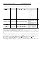
In particular this command will produce (for a blue frame and central wavelength 346 nm)
the following files:
frame
drs setup BLUE.tbl
b346BLUE.tbl
l346BLUE.tbl
o346BLUE.tbl
DO CLASSIFICATION
DRS SETUP BLUE
BACKGR TABLE BLUE
LINE TABLE BLUE
ORDER GUESS TAB BLUE
meaning
calibration table
background table
line table (guess solution)
order table (guess solution)
At this point the ECHELLE context parameter NBORDI is equal to zero. This means that
an automatic determination of the orders is performed.
In principle one could also pass reference frames through a catalogue and give the command
Midas> PREDICT/UVES format TAL b.bdf predictI.cat predictO.cat
where predictI.cat is an image catalog which must contain the line reference table. In this
case the output names given above will be present after data reduction in the output catalog
predictO.cat. The line table l346BLUE.tbl is the ”Guess Solution” and will be classified (in
our case) in the catalog as LINE TABLE BLUE.
UVES data reduction cookbook
4
VLT-MAN-ESO-13200-4033
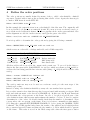
4
Define the order positions
The order positions are usually defined by means of the so called order flatfields – flatfield
exposures obtained with a narrow slit producing thin echelle orders. Again, the first step is
to make a BDF frame from the FITS file.
Midas> SPLIT/UVES order FF.fits
In this example the order FF.fits is an order flatfield of the blue arm. The output file will
be stored in the local directory as order FF b.bdf. We can now create a reference catalog to
store all the needed calibration frames. To allow a pipeline check on the guess and final order
tables alignment we add also in the reference catalogue the guess order table:
Midas> crea/icat refB.cat o346BLUE.tbl DO CLASSIFICATION
Now it is possible to determine the order positions by giving the following command:
Midas> ORDERP/UVES order FF b.bdf refB.cat refB.cat
which creates an order table, a background table, and a DRS setup table.
frame
DO CLASSIFICATION
o346 2x1.tbl
ORDER TABLE BLUE
b346 2x1.tbl
BACKGR TABLE BLUE
d346 2x1.tbl
DRS SETUP BLUE
l346BLUE.tbl LINE TABLE BLUE
meaning
Order table
Background table
DRS setup table
Line Guess table
All these tables will be stored in the output catalog refB.cat. To proceed in the data reduction the line guess table (l346BLUE.tbl, in our case, which we rename as l346 2x1.tbl to
evidence the bin setting) and the line reference table (thargood 3.tbl) should be added to this
catalog.
Midas> -rename l346BLUE.tbl l346 2x1.tbl
Midas> ADD/ICAT refB.cat l346 2x1.tbl
Midas> ADD/ICAT refB.cat thargood 3.tbl
The catalog refB.cat may now be used as a reference catalog for the next steps of the
reduction procedure.
Instead of using order definition flatfields you may also use standard star exposures.
It is worth to mention here that this step has been performed without using a reference DRS
table and with automatic order detection (NBORDI=0). In this case, the Hough Transform
will determine the orders present on the frame. In case of low photon level in part of the
order definition frame, this step may underestimate the number of orders. To have a complete
determination of the orders one should visually check that the number of determined orders
corresponds to the one present on the frame. If not, it is better to manually set this number
(No) using the command SET/ECHELLE NBORDI=No before giving the ORDERP/UVES
command. The UVES pipeline indeed uses the results of the physical model which predicts
the geometrical spectral format and thus also the number of orders which should be present
on the frame. This value is stored in the DRS setup table when the first guess solution
UVES data reduction cookbook
VLT-MAN-ESO-13200-4033
5
is generated. This method is appropriate for the standard setting, and is more robust and
uniform than doing an automatic order detection. But in case of a non standard setting, it
may well be that due to non-uniform light distribution on the detector (induced by filters
eventually present along the light path) the predicted number of orders is greater than the
detected one. In this case, using the value of NBORDI contained in the DRS setup table
generated from the physical model would lead to an overestimation of the number of orders
and to a wrong solution. For this reason, in pipeline releases after version 1.0.2 a quality check
on the predicted vs. detected spectral format has been introduced. The expected number of
orders can be also set manually (SET/ECHELLE NBORDI=No).
5
Wavelength calibration
For the wavelength calibration you will need a ThAr-lamp exposure, a line reference table,
and first guess solutions (order table and line table) which allows the automatic mode of the
UVES command WAVECAL/UVES. The interactive mode may be enforced by its mode parameter.
The ThAr-lamp exposure may be obtained using the observation template UVES < mode > y
(< mode >= blue, red, dic1, dic2, y=wave, wavefree).
Again, at first you have to transform the original input file by:
Midas> SPLIT/UVES b346 TAL.fits
Assuming b346 TAL.fits as an exposure of the blue arm, the output from this command
will be used as the input file of the wavelength calibration command.The next UVES context
MIDAS command uses, for simplicity, the input reference catalog name as the output catalog
(refB.cat):
Midas> WAVECAL/UVES b346 TAL b.bdf refB.cat refB.cat AUTO
This command performs the wavelength calibration using the following default options:
parameter
P4
P5
P6
P7
P8
value
AUTO
yes
Y/[N]
Y/[N]
[+]
purpose
the previously determined line table from refB.cat is used
the procedure generates the resolution plots
performs (Y/[N]) the wavelength calibration only at order center
produced output FITS file
see on line help of command (this parameter control offset
and extraction window of object and sky for wavelength
calibration solution)
This step generates the line tables for each slit window (sky, object, sky) which will be stored
in the output catalog, refB.cat, and updates the DRS SETUP x (x=BLUE in our example)
table
UVES data reduction cookbook
frame
l346 2x1 1.tbl
l346 2x1 2.tbl
l346 2x1 3.tbl
d346 2x1.tbl
DO CLASSIFICATION
LINE TABLE BLUE1
LINE TABLE BLUE2
LINE TABLE BLUE3
DRS SETUP BLUE
VLT-MAN-ESO-13200-4033
6
meaning
line table lower sky
line table object
line table upper sky
DRS Setup Table
As the ThAr line reference list is no a product of the UVES context you have to ensure that
the descriptor ESO.PRO.CATG is set to LINE REFER TABLE (READ/DESC, WRITE/DESC).
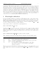
6
Master calibration files
Master calibration frames – master bias and master flatfields – are used for the science reduction. They are stacked median averages of a set of input frames. They are created by the
command MASTER/UVES. To keep the data reduction simple, we collect all the bias frames in
an image catalog:
Midas> CREATE/ICAT biasB.cat bias346 *.fits
At first the set of input frames have to be transformed into the standard orientation (wavelength increases from left to right and from bottom to top) and into the MIDAS BDF-file
format by means of:
Midas> SPLIT/UVES biasB.cat split bias.cat
The transformed data will be stored in the output catalog split bias.cat. Having prepared
the input data one can give the command:
Midas> MASTER/UVES split bias.cat refB.cat
which produces a master frame for each configuration (blue, red arm lower and upper part),
i.e. you may use a mixed set of input frames (e.g.: blue bias frames, red bias frames lower and
upper part 5 frames each – as a result you will get 3 master biases.). All products will be stored
in the output catalog which again for simplicity has the same name as before (refB.cat).
This command will produce a master bias frame:
frame
mbBLUE 2x1 b.bdf
DO CLASSIFICATION meaning
MASTER BIAS BLUE Master Bias frame
and its name will be added to the reference catalog.
For the flatfields and as before, for simplicity, we put all the Flat Field frames in one catalog:
Midas> CREATE/ICAT ffB.cat ff346 *.fits
Midas> SPLIT/UVES ffB.cat split ff.cat
UVES data reduction cookbook
VLT-MAN-ESO-13200-4033
7
The master Flat Field is saved in the usual catalog (refB.cat).
Midas> MASTER/UVES split ff.cat refB.cat refB.cat
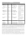
The products of this step are (in our case of BLUE arm data, binning 2x1, slit length = 8
arcsec) the following frames:
frame
DO CLASSIFICATION
mf346 2x1 s08 b.bdf MASTER FLAT BLUE
av346 2x1 s08 b.bdf
bg346 2x1 s08 b.bdf
meaning
master FF
average FF
bkg
The master Bias is subtracted from the master flatfield (default option M of P4) and no dark
is subtracted. One can also subtract a constant bias level (in this case P4=number) this bias
level (number) can be determined with STATISTIC/IMAGE on different portions of the bias
frames. An inter-order background is also determined and subtracted to the Flat Field frame
(the parameter P6 sets the method) The master flat frame is added to the reference catalog.
Midas> MASTER/UVES split ff.cat refB.cat refB.cat 120
This example assumes a constant bias of 120 counts used for the master flatfield creation.
Furthermore, the master flats will be background subtracted which requires appropriate background tables and DRS setup tables (to be present in the catalog refB.cat) – products of
ORDERP/UVES.
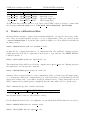
7
Science frame reduction
The science reduction for UVES supports different modes controlled via additional parameters:
ffmode Flatfielding may be done in the pixel-pixel space (P) as well as in the extracted
pixel-order space (E).
extract The extraction of the object may be performed as a simple average (AVERAGE) or
by the optimal extraction method (OPTIMAL). The number of ‘rows’ to be averaged per
order is defined by the MIDAS keyword SLIT.
bmeasure The inter-order background subtraction is based on the ‘measurements’ on the
grid of background positions. For each background position the median (MEDIAN) or
the minimum (MINIMUM) within a certain window will be used as the measurement at
that point. In case of very narrow inter-order space the minimum method could produce better background images as otherwise the measurements could be contaminated
by neighboring orders. Usually the method MEDIAN gives better results than the MINIMUM.
From version 2.0.0 spectra merging can be controlled via parameter P8 which may have 4 components: merge method, delta set switch, delta1, delta2. merge method is the method
used to merge spectra: OPTIMAL or AVERAGE. delta set switch is a parameter used
to set:
UVES data reduction cookbook
VLT-MAN-ESO-13200-4033
8
D: Default delta setting (as was in previous pipeline releases, for BLUE arm delta1=delta2=3,
for RED arm delta1=delta2=5).
A: Automatic setting of deltas. Appropriate deltas are chosen for each instrument
setting. See on line help.
U: User defined deltas. In this case are taken the values of delta1 and delta2 as specified
by the user.
delta1: user specified value of delta used to merge the blue edge of the spectra. delta2:
user specified value of delta used to merge the red edge of the spectra.
The possible parameter values are shown in brackets (). As usual, at first you have to transform your science frame:
Midas> SPLIT/UVES sc.fits split sc.cat
We can reduce the data giving the following UVES context MIDAS command:
Midas> REDUCE/UVES split sc.cat sc redB.cat refB.cat E OPTIMAL MEDIAN
In this case we use P4=E meaning that the Flat Fielding is done in the pixel-order space
during extraction. In case of data taken in the far Red (wcal=860), to better correct for the
fringing effect one could apply the P method, i.e. doing the Flat Fielding before extraction in
the pixel-to-pixel space.
P5=OPTIMAL means we choose optimal extraction. This method has been proven to give
good quality for low-to-medium signal to noise (S/N) ratio science objects. For very high S/N
it is suggested to use the average extraction method. The optimal extraction may show quality
problems appearing as sudden spikes on the spectra. This occurrence can be confirmed also
looking at the ”weight.bdf” weight image which for a successful extraction should appear uniform with only a few randomly scattered ”holes” corresponding to detection (and suppression)
of cosmic rays. If instead significant portion of holes in the weight image with a periodicity
are noticed, this means that this step has failed and one should use average extraction.
P6=MINIMUM/[MEDIAN] is the background estimation method.
See help SUBTRACT/BACKGROUND for clarification.
Proper setting of parameter P7 allows one to chose (if used P7=N,N,N) one’s own setting
respectively for the offset, slit, skywind setting. This allows one to use UVES/REDUCE to
reduce more than one source on the slit, interactively determining (LOAD/IMA, LOAD/ECH,
GET/CURS) and setting (SET/ECHELLE) the values of the three involved parameters. Default setting for P7 is Y,Y,Y which means automatic determination of the three parameters.
To use OPTIMAL extraction with multi sources the real keyword OBJSET has to be appropriately set (see more in section 13).
The command REDUCE/UVES will reduce every science frame stored in the input catalog using
the appropriate calibration frames from the reference catalog refB.cat. So, for each configuration there has to be a complete reference set. In this example, there has to be two sets – one
for the lower red and one for the upper red arm. In principle you are able to mix blue and red
arm exposures for the science reduction process.
Finally, all products will be stored in the output catalog sc redB.cat. The following data
products will be created (only the products of the lower CCD (EEV) of the red arm are shown
UVES data reduction cookbook
VLT-MAN-ESO-13200-4033
9
– in principle they are always the same for the other configurations):
Filename
r rbf 0 l.bdf
Format
1D (wav)
m rbf 0 l.bdf
1D (wav)
w xb rbf 0 l.bdf
2D (wav-ord)
wfxb rbf 0 l.bdf
2D (wav-ord)
errmrbf 0 l.bdf
1D (wav)
var rbf 0 l.bdf
1D (pix-ord)
Description
extracted,
flatfielded,
wavelength calibrated
merged, sky subtracted
science frame
MERGED SCI POINT REDL
extracted,
flatfielded,
wavelength calibrated,
merged,
science frame
WCALIB SCI POINT REDL
extracted, wavelength
calibrated science frame
WCALIB FF SCI POINT REDL extracted,
flatfielded, wavelength
calibrated frame
ERRORBAR SCI POINT REDU standard deviation of
reduced science frame
VARIANCE SCI POINT REDU variance of flatfielded,
extracted science frame
ESO.PRO.CATG
REDUCED SCI POINT REDL
reduced: debiased, inter-order background subtracted, flatfielded, re-sampled, merged and sky subtracted data.
merged: merged orders, no sky subtraction (one dimensional).
wavelength calibrated: re-sampled extracted orders.
sky: sky contribution is determined from the two sky windows below (sky(1)) and above the object (sky(2)) in
each order. For the optimal extraction the weights used for the object extraction are applied to the averaged
sky.
From pipeline release 1.3.0 on are also created, in case of optimal extraction, frames with optimally extracted
sky. These contains in the frame name the sequence opt sky . The second column of the table shows the
hierarchical FITS header keyword for the product category. By means of this keyword the products may easily
be identified. The MIDAS output catalog uses this keyword as identifier field. In case of the upper CCD of
the red arm the category extension REDL changes to REDU and for the blue arm to BLUE.
The prefix of the filenames also immediately shows the different product types:
w: wavelength calibrated, f: flatfielded, x: extracted, b: background subtracted data file. The prefix m
indicates merged data which are implicitly always ‘wfxb’ data.
UVES data reduction cookbook
VLT-MAN-ESO-13200-4033
Filename
w xb sky REDL1.bdf
Format
2D (wav-ord)
ESO.PRO.CATG
WCALIB SKY1 REDL
wfxb sky REDL1.bdf
2D (wav-ord)
WCALIB
m sky REDL1.bdf
1D (wav)
MERGED
w xb sky REDL2.bdf
2D (wav-ord)
WCALIB
wfxb sky REDL2.bdf
2D (wav-ord)
WCALIB
m sky REDL2.bdf
1D (wav)
MERGED
m sky REDL.bdf
1D (wav)
MERGED
w xb rbf 8.bdf
1D (wav)
WCALIB
w xb1 rbf 8.bdf
2D (wav-ord)
WCALIB
w xb2 rbf 8.bdf
2D (wav-ord)
WCALIB
10
Description
extracted, wavelength
calibrated sky(1) frame
FF SKY1 REDL
extracted, flatfielded and
wavelength calibrated
sky(1) frame
SKY1 REDL
extracted,
wavelength calibrated,
flat fielded,
merged sky(1) frame
SKY2 REDL
extracted, wavelength
calibrated sky(2) frame
FF SKY2 REDL
extracted,
wavelength calibrated,
flatfielded
sky(2) frame
SKY2 REDL
extracted,
wavelength calibrated,
flat fielded,
and merged sky(2)
frame
AV SKY REDL
extracted, flatfielded,
wavelength calibrated,
merged, average of
sky(1) and sky(2)
frame
FLAT OBJ REDL
extracted, wavelength
calibrated, flatfield
of the object
FLAT SKY1 REDL extracted, wavelength
calibrated flatfield
FLAT SKY2 REDL of the two sky windows
Note also that with automatic determination of the offset,slit,skywind parameters (P7=Y,Y,Y),
it may happen that due to a big value of the object offset, automatically determined during
data reduction, one sky window is less than 4 pixels wide so that the data reduction procedure
automatically switches to one (from a default value of two) sky extraction window. See also
the help of the command REDUCE/UVES for more information on how to properly set user
defined extraction parameters in case of optimal extraction.
For operational purposes, from pipeline version 1.1.1 on, we have decided to produce ”dummy”
solutions also relative to the extraction window which is automatically suppressed. This is to
keep the same order in the pipeline data products. Such solutions, which have no physical
meaning, are labeled with the prefix ”dummy” in the file name. The real solutions are as
before the one obtained considering only the ”good” sky extraction window.
The errorbar image (filenames having prefix errm) is obtained as the square root of the variance
frame (varm...). The variance frame is calculated considering the contribution from the read
out noise and from the source. In case of average extraction this is calculated per pixel.
The variance of the flat fielded object is next given propagating the variance for the ratio
UVES data reduction cookbook
VLT-MAN-ESO-13200-4033
11
(extracted object)/(extracted flat field). In case of optimal extraction an input variance is
calculated as described above. This will follow transformations similar to the flux until in the
end after having evaluated the best Gaussian cross order profile coefficients, it is evaluated
for each X point the chi-square between a normalized Gaussian times a variable amplitude
(to which is added the found background) and the actual spectra doing the quadratic sum
along the cross order direction and using as weight the input variance. For a number of values
of amplitudes one gets corresponding values of chi square. Assuming that the chi square as
a function of the amplitude is a parabola near the minimum, one can calculate which is the
change in amplitude that generates a unitary increase of the chi square. This change can be
assumed as an error associated with the amplitude and from this one can get an estimate of
the variance associated to the optimal extraction process. Clearly this variance value depends
on how good is the Gaussian model approximation assumed from the cross order profile.
Up to version 2.9.7, optimal extraction was having problems (apparent strange ripples and
patterns within an order on a few pixel scale) in particular for high S/N data (greater than
around 50). Those problems were solved in the latest version. For very high S/N (¿ 200) data,
the user may still want to use the average extraction. Remember also that Average extraction,
as suggested by the name, makes an average of the extracted signal along the extraction slit.
So the intensities of data reduced with optimal and average extraction differ approximatively
by a factor equal to the slit size in pixel. Flux calibrated merged spectra may be generated
if a master response frame is added in the input reference catalog. In this case using average
extraction the products have same units as the ones generated using optimal extraction.
Because it is difficult to model the light profile coming from the image slicer and to estimate
the sky contribution from the image slicer, data should be extracted with AVERAGE method
and NO sky subtraction. For this instrument setting during science spectra extraction the
pipeline recognizes if the frame has been created using an Image Slicer and in such a case it
is automatically set to the relevant extraction parameters (object extraction slit, extraction
method, sky subtraction option).
Optimal extraction quality has been improved a lot in the latest release. We can now prudently
say that usually the extraction quality is quite good. It is important to check it using the
command
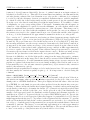
Midas> MPLOT/CHUN [order trace x] [half size y] [switch]
where x=BLUE,REDL or REDU, half size y is half size in bin units of the plots in Y direction,
and switch can assume values pos(ition) or fwhm, respectively for the plots of the cross order
chunk position or FWHM distributions. These plots display in black the values of the raw data
(pos/FWHM) for each chunk, in green the values predicted from the first fit after some precleaning of outliers, in blue the last fit after k-sigma clipping of residual outliers and in magenta
are shown the points used to determine the last fit. Good extraction is typically reached when
the black points are well fit by the blue ones. As the plots show, the point distribution has
usually a well aggregated parabolic distribution with sloppiness and curvature typically of a
small fraction of pixel. So in general, the fit for position and FWHM is parabolic. In case the
data distribution is not well aggregated (this may happen for particularly low S/N data) it
might happen that the fit gives too big values for the sloppiness and the curvature. To prevent
such a problem thresholds and checks on these parameters are set in the code so that if the fit
is not very good and the parabola fit parameters are wrong the fit is switched first to linear and
eventually to uniform. The linear (or even uniform) approximation is a safer approximation
than a parabolic one to fit a highly scattered point distribution. The user should always check
to have a reasonably good fit (max scatter in y bin should be 0.1-0.3 bins).
UVES data reduction cookbook
VLT-MAN-ESO-13200-4033
12
Having a proper master response frame (provided by DFO) and adding it in the input reference
catalogue one could also produce flux calibrated merged spectra (having prefix flx ).
8
Calibration scripts
In order to make life a bit easier, three additional MIDAS procedures exist, which may help to
fill your calibration database for later science reduction. The first command PREPARE/CALDB
puts all the calibration commands mentioned before together into one script so that one has
only to create an input catalog for a certain UVES setting and pass it to this procedure.
First, one collects in an image catalog all the main calibration fits files:
1. raw formatcheck frame (‘fits’)
2. raw order definition flatfield (‘fits’)
3. ThAr lamp exposure (‘fits’)
4. raw list of biases (‘fits’)
5. raw list of flat fields (‘fits’)
And apply SPLIT/UVES to get the data in the proper format and orientation:
Midas> CREA/ICAT raw fits.cat *.fits
Midas> SPLIT/UVES raw fits.cat raw split.cat
Next, one prepares a catalog refer.cat containing the ThAr line reference table in the MIDAS
format:
Midas> INDISK/FITS thargood 3.tfits thargood 3.tbl
Midas> CREA/ICAT refer.cat null DO CLASSIFICATION
Midas> ADD/ICAT refer.cat thargood 3.tbl
Finally one applies the PREPARE/CALDB script with the following syntax:
Midas> PREPARE/CALDB raw split.cat refer.cat
Assume one has created an input catalog for binned data (2×1) of the central wavelength
346 nm then after having executed the script one will get at the end all the necessary calibration solutions which are listed in an output catalog ref346 2x1.cat. Use
Midas> SAVE/CALDB ref346 2x1.cat /data/caldb
to store the solutions in one’s calibration database.
The third command allows one to retrieve the complete set of calibration frames from the
calibration database:
Midas> GET/CALDB ref346 2x1.cat /data/caldb
UVES data reduction cookbook
VLT-MAN-ESO-13200-4033
13
in order to be well prepared for the science reduction:
Midas> REDUCE/UVES sc346 2x1 b.bdf sc346.cat ref346 2x1.cat E OPT MED
For more details and additional options please read the on line help of the commands.
9
UVES data display and hardcopy
The echelle data may be displayed using the command PLOT/UVES. For a detailed description
please see the help file (HELP PLOT/UVES).
Midas> PLOT/UVES extract.bdf 1,13 0,100 ‘‘title’’ extract.ps
Furthermore, a hardcopy utility is provided: HARDCOPY/PLOT especially for hardcopies of the
image displays as the usual hardcopy command COPY/DISP only properly works for non-covered
displays.
Midas> HARDCOPY/PLOT P ff 346.ps ff 346.bdf
This will produce a postscript hardcopy (ff 346.ps) of the input file ff 346.bdf. Additionally, the main characteristics will be printed at the bottom of the plot. By default, the
hardcopy facility is disabled. You may enable it doing:
Midas> HARDCOPY/PLOT ON
Use OFF instead of ON in case you wish to disable hardcopies. This may be useful, as some
UVES commands are sensible to the hardcopy command status.
10
Saving the keyword setup
The keywords used during the reduction of the data may/should be saved in a so called data
reduction system setup tables (DRS tables). These are classified products which may be identified by the UVES commands. These tables control the whole reduction process. If you are
changing some of the ECHELLE context keywords using SET/ECHELLE you should store these
changes for later use in a DRS table:
Midas> SAVE/DRS drs 346.tbl
This call will save all ECHELLE keywords in the MIDAS table drs 346.tbl as MIDAS descriptors, existing DRS tables will be overwritten.
UVES data reduction cookbook
11
VLT-MAN-ESO-13200-4033
14
Message level
The output of information is reduced to a minimum for use of the UVES context within the
pipeline infrastructure. When using the context in an interactive mode it could be helpful to
get some more information. In this case you may control the message level by:
Midas> VERBOSE/OUT VERY
Instead of VERY you may use ON or OFF which switches back to the default message level or,
even more, switches all the messages off except for warnings and error messages.
12
Automatic preparation of calibration solutions
To quickly prepare calibration solutions with default parameter settings, it is worth to describe
the use of the script uves popul.sh, included as part of the distribution in $PIPE HOME/uves/uves/scripts/
directory (which should be included in your local PATH).
This script can be executed from any shell with the following syntax (we suppose to be in the
directory where the raw FITS files are located):
$PIPE HOME/uves/uves/scripts/uves popul.sh raw fmtchk.fits raw orderpos.fits raw wavecal.fits
raw bias*.fits raw flat*.fits ThAr ReferLineTable.fits
where the input raw data refers to a coherent instrument setting (same instrument arm, mode,
central wavelength and binning); the script starts a MIDAS session and produces results in
the directory
$HOME/midwork/tmpwrk/
In particular this creates a subdirectory: $HOME/midwork/tmpwrk/data/ which contains all
the calibration solutions.
Moreover in $HOME/midwork/tmpwrk/ the files xORDER.tbl, xLINE.tbl, xBACKGR.tbl
will be present to be used as input reference of the MIDAS command INIT/ECHELLE x
(x=BLUE or REDL, REDU). This command sets up all the important keywords of the echelle
environment.
The uves popul.sh is a script which executes the procedure uves prepcalib.prg. This procedure
executes in series all the main UVES pipeline reduction steps involved in the calibration data
analysis. Mainly it executes the command CONFIG/INSTR on the reference catalog to get,
set or check: mode, the detector involved, the central wavelength, the binning factor, if a
dichroic is inserted.
Next, it executes the first main data reduction step: it runs the physical model to determine
the geometrical predicted spectral format, a first guess solution for the line (dispersion relation)
and the order tables and generates a first DRS SETUP table; if a reference formatcheck frame
(MASTER FORM x, x=BLUE or REDL, REDU) is provided it also does a QC stability
check.
These data (ORDTAB, DRSTAB) are used in the following data reduction step, the order
position determination (ORDERP/UVES). In this step an Hough Transform is performed
to determine the order positions. Initially it is given (through a SAVINI/ECH DRSTAB
UVES data reduction cookbook
VLT-MAN-ESO-13200-4033
15
READ command) as parameter to DEFINE/HOUGH the number of orders as predicted by
the physical model (previous step). In standard configuration settings, this number usually
coincides with the actual number of orders on the detector. On particular non standard
configurations, due to the presence of some filter along the path, it may be possible that the
detector illumination may drop to almost zero on some regions and for this reason the detected
number of orders is lower than the one predicted by the physical model. For this reason the
order position procedure always does a quality control check (check the standard deviation
of the :RESIDUAL column in the order table which may have a jump in case the predicted
number of orders is greater than the detected one) and eventually iteratively decrease the
number of orders given as input parameter to DEFINE/HOUGH.
Finally the ORDER, BACKGR and DRS SETUP tables are produced. The following step is
the wavelength calibration (WAVECAL/UVES). Next the Master bias and the Master Flat
frames are created. To use the calibration database data in an interactive MIDAS section, for
example to reduce a science frame, one has to convert the FITS data to MIDAS format.
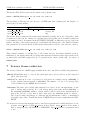
13
Reduction of more than one object source on the slit
The UVES pipeline has been designed to do automatic data reduction of point-like sources
well centered on the slit. Some users may be interested to observe and reduce data of more
than one object on the slit. For this purpose we have upgraded some commands to allow the
user to interactively perform a proper extraction. This is still possible in a manual session
using the UVES context. Here we give a small example which may be adapted to the user’s
needs.
Let’s suppose the user has on the slit two adjacent spectra. Let’s suppose the user has used
the uves popul.sh to prepare all the data calibrations. During this step the echelle fundamental data tables are also produced: yORDER.tbl, yLINE.tbl, yBACKGR.tbl (y=BLUE or
REDU,REDL).
Let’s suppose these tables, the calibration solutions and the science raw data to be reduced
are available in our directory (here for example indicated with raw sci two sources x.bdf).
We would give the following commands:
Midas> SPLIT/UVES raw sci two sources x.bdf
Midas> INIT/ECHE y
Midas> LOAD/ECHE
Midas> GET/CUR
With this last command you overplot the detected order trace to have a reference to get
the extraction parameters offset, slit, skywind (this last for average extraction).
were x=b or x=l, x=u and y=BLUE or y=REDL, y=REDU respectively for the BLUE or REDL,REDU
chip.
So you can calculate the values of off, slit, skywind (skywind in general is a 4 component parameter: skywind=skyw(1),skyw(2),skyw(3),skyw(4)), for each of the object to be extracted.
Midas> SET/ECHE offset=off1 slit=slit1 skywind=skywind1
Midas> SAVINI/ECHE drstab.tbl
Midas> REDUCE/UVES raw sci two sources x.bdf out.cat ref.cat E A MED N,N,N
UVES data reduction cookbook
VLT-MAN-ESO-13200-4033
16
Where drstab.tbl indicates the drs setup table being used. Here we use P7=N,N,N meaning
we have dis-activated (N) the automatic setting respectively of the offset,the slit, and the skywindow (used in average extraction) values, and used the corresponding values set manually
(SET/ECHE). We have also saved our setting in the drs setup table. In our case we have used
average extraction, but we could also use optimal extraction. Similarly the other object can
be reduced.
It is probably useful to write some more here in case the user would like to extract two sources
on the slit using optimal extraction and a manual setting of the extraction parameters.
For simplicity we start the discussion with the extraction of a single source. This case is
typically treated in an automatic way by the pipeline. The discussion helps to understand
the meaning of each relevant parameter, also for the more general case in which one has to
extract more than one object, case in which automatic extraction would fail.
Be obj trace the position of the object as measured (LOAD/IMA LOAD/ECHELLE GET/CUR)
with respect to a reference position (for example the order trace).
Be ord trace the position of the order trace.
Be offset the offset chosen for the extraction, this being the center of the extraction slit
(slit ext).
The parameter objset, used in the optimal extraction, is the distance of the object from the
center of the extraction slit slit ext. It is used as first guess to start the Gaussian fit of
the object’s light distribution cross order profile within the extraction slit. Next the optimal
extraction algorithm searches automatically for the best object position to achieve within an
order an overall best fit of the cross order profile.
These parameters are related by the following relation
offset+objset=obj trace-order trace
The slit of integration will be centered at the position order trace+offset.
The user could get such a formula, taking into account the previous information, for example
doing a plot, in which one has, for a numerical example an object trace at position 40, an
order trace at position 20 and the extraction slit centered at position 25. Let’s also suppose
that one would like to have an extraction window of 36 pixels.
We have chosen this sequence as it is simpler and all the parameters are positive.
With our numbers objset=object trace-order trace-offset=40-20-(25-20)=40-20-5=15
which is actually what one can measure on a scaled plot.
Obviously objset and offset have a sign and the situation can change: If one puts the
integration slit below the order trace the offset will be negative. Similarly one can have a
situation for which objset is negative.
To make things easier, if the extraction window is centered on the object (this means objset=0),
the parameter offset measures the distance of the object trace from the order trace, which
is exactly what one would imagine.
When is all this important? Usually one will have only one object in the slit and in such
a case offset is automatically determined by offset/echelle so that one can take objset=0
(as the pipeline does in default mode) and the optimal extraction will start to search for the
object at the slit center without any problem.
A more interesting case happens when there is more than one object in the (full) slit, and in
particular if the two sources are very close to each other (as may happen for traces of lensed
quasars or in a binary system). Obviously one does not want to use a slit covering both objects
UVES data reduction cookbook
VLT-MAN-ESO-13200-4033
17
otherwise the spectral information coming from the two spectra will be mixed (moreover doing
so the optimal extraction would get crazy trying to fit both traces). It is also suggested not to
have a small integration window centered on each object (objset=0), as probably one would
cut-off part of the object and/or not well estimate the sky.
In such a case it is better to chose an offset and an integration slit such that the slit includes
one object (but not the adjacent) and a lot of sky on one side of the object. It is not a
good idea to have in this case objset=0 and leave the optimal extraction search for the object
position as in this particular situation the object will be near the slit border and the algorithm
may not be clever enough to find the object. For this reason one has to specify objset, the
starting offset with respect to the slit center. Following these indications and choosing an
extraction slit size such that at least three pixels are left on each side of the object, one can
iteratively do optimal extraction of all the sources.
If all is done correctly in the setting of these parameters, one can notice that the object position
reported by the optimal extraction at each order varies slightly with the order position and it
is quite close to the value slit ext/2+objset set from the user.
It is always a good practice, after optimal extraction, to use the command MPLOT/CHUN
to display the trace object positions (or FWHM) as a function of X and verify that a good
fit was obtained. It is only necessary to check one trace. This means that the extraction slit
includes only one object. Moreover the magenta points should fit well to the dark ones, this
being an indication of a good extraction.
Another interesting test one could do is to get the best combination of parameters to have
a reasonable extraction, and next, satisfying the formula above, move the extraction window
until the object exits from it. At this point the optimal extraction will start to have problems
giving warnings like:
Warning: IMASK COUNTER LESS THAN 10
meaning that only a small number of chunks are left after a k-sigma clipping step over position
(or FWHM values), a situation typical of very low S/N data, even more if no signal is in the
extraction window as it can happen at a certain point in the proposed exercise.
In such last case the plots from MPLOT/CHUN (and of the extracted spectra) will be much
worse..
After such explanations we add only how, in practice, we could activate such settings, using
the numbers given.
Midas> SET/ECHE offset=5 slit=36
Midas> write/key objset/r/1/1 15
Midas> SAVINI/ECHE drstab.tbl
Midas> REDUCE/UVES raw sci two sources x.bdf out.cat ref.cat E O MED N,N,N
Midas> MPLOT/CHUN order trace y.bdf 3 obj
Midas> MPLOT/CHUN order trace y.bdf 3 fwhm
where x=b or x=l, x=u and y=BLUE or y=REDL, y=REDU respectively for the BLUE or REDL,REDU
chip. Here we have also reported the command to check, after extraction, the quality of the
order tracing.
UVES data reduction cookbook
14
VLT-MAN-ESO-13200-4033
18
Reduction of extended sources
The possibility to do simple reduction of extended sources has also been included on the
pipeline version 1.0.6 on. In this case the source is extracted with a 1 bin extraction slit and
a variable offset scanning the full length of the observation slit. So the order is rotated-flat
fielded, wavelength calibrated and finally merged. The command to be used is:
Midas> REDUCE/SPAT split.cat out.cat ref.cat BckMeasMeth,FfMeth,MerMeth
MerSwitch,delta1,delta2
split.cat is an input image catalog with images to be reduced oriented in the proper way
(SPLIT/UVES), for example the one produced as described in the normal data reduction
for science data. out.cat is an output image catalog produced from the pipeline. ref.cat
is the reference catalog for science data reduction produced as described in the section for
normal data reduction. BckMeasMeth is the background measurement method (MIN, MED,
see help subtract/background) FfMeth is the flat fielding method, which can assume values
“E”, “P” or “N” with the same meanings as the corresponding parameter in the command
REDUCE/UVES. MerMeth is the merging method, which can assume values “O” (Optimal),
“A” (Average), “N” (Noappend), with similar meaning as for the standard MIDAS command
MERGE/ECHELLE.
We suggest not to use REDUCE/SPAT after having used on the same data REDUCE/UVES.
In fact after the flat fielding or the background have been applied on the science frame
the pipeline sets given descriptors so that it can recognize that the corresponding operation does not need to be repeated. If the user has already processed a science frame with
REDUCE/UVES the science frame may be already background and flat field corrected (if
the flat field correction has been performed pixel to pixel), thus the user may not be able to
choose and do the proper background and flat field methods offered by the REDUCE/SPAT
command itself.
Default values for parameter P4 are MED, E, A. One could use as MerMeth “O” to have a
better behaviour in the overlapping region between one order and the next, or if not satisfied,
the Noappend option to have each order in one corresponding image file.
MerSwitch is the parameter controlling the setting of deltas used in the merging of the spectra.
It can have values D (Default), A (Auto) or U (User-defined) which have the same meaning
as the corresponding subparameter of parameter P8 in REDUCE/UVES command. Delta1
controls the amount of overlapping considered in the merging of the blue edge of a spectra.
delta2 controls the amount of overlapping considered in the merging of the red edge of a
spectra. Using option A the pipeline will use predefined delta1 and delta2 parameter values.
As those parameters affect significantly the quality of merged spectra we suggest the user to
use the U option and choose appropriate values for delta1 and delta2. See also on line help of
parameter P5 for command REDUCE/SPAT
Blue data, for setting 346, might be better reduced using a NO flat fielding mode, because
in the short wavelength range of this setting, the flat field data might have been taken in
non-appropriate conditions. This rarely happens as LN2 lamps with a proper behaviour are
being used.
The products generated by this procedure are the following: If p1 is the MIDAS procedure
parameter specifying the input frame:
• xb2d {p1} is the background subtracted, extracted (rotated), frame,
UVES data reduction cookbook
VLT-MAN-ESO-13200-4033
19
• fxb2d {p1} is the background subtracted, extracted (rotated) flatfielded, frame,
• wfxb2d {p1} is the background subtracted, extracted (rotated) flatfielded, wavelength
calibrated frame,
• mwfxb2d {p1} is the background subtracted, extracted (rotated) flatfielded, wavelength
calibrated, merged frame.
In case ”Noappend” the merging option is chosen, the procedure generates an image frame
per each order with indexed names such as the following:
mwfxb2d {p1}0001....mwfxb2d {p1}00NN, where NN is the number of extracted orders. This
last option may be used if the user has not found proper values of delta1 and delta2 parameters.
15
Session example: Blue Data
We refer now to a case of BLUE arm data with wcent=346 nm and 2x1 binning.
15.1
Default Display Initialization
Midas> CONFIG/DISP 1600 1200 0.6
15.2
Predictive Format Determination
Midas> SPLIT/UVES frmtChk346 TAL.fits
Midas> INDISK/FITS thargood 3.tfits thargood 3.tbl
Midas> PREDICT/UVES frmtChk346 TAL b.bdf thargood 3.tbl
15.3
Order Position Determination
Midas>
Midas>
Midas>
Midas>
Midas>
Midas>
crea/icat refB.cat o346BLUE.tbl DO CLASSIFICATION
SPLIT/UVES order ff346.fits
ORDERP/UVES order ff346 b.bdf refB.cat refB.cat
-rename l346blue.tbl l346 2x1.tbl
add/icat refb.cat l346 2x1.tbl
add/icat refb.cat thargood 3.tbl
15.4
Wavelength Calibration
Midas> SPLIT/UVES wcal346 TAL.fits
Midas> WAVECAL/UVES wcal346 TAL b.bdf refB.cat refB.cat AUTO yes
15.5
Master Bias Determination
Midas> CREATE/ICAT biasB.cat bias346 *.fits
Midas> SPLIT/UVES biasB.cat split biasB.cat
Midas> MASTER/UVES split biasB.cat refB.cat
UVES data reduction cookbook
15.6
VLT-MAN-ESO-13200-4033
Master Flat Determination
Midas> CREATE/ICAT ffB.cat ff346 *.fits
Midas> SPLIT/UVES ffB.cat split ff346.cat
Midas> MASTER/UVES split ff346.cat refB.cat refB.cat
15.7
Science Reduction
Midas> SPLIT/UVES sc 346.fits
Midas> REDUCE/UVES sc 346 b.bdf reducedB.cat refB.cat E O MED
16
Session example: Red Data
We refer now to a case of RED arm data with wcent=580 nm and 1x1 binning.
16.1
Default Display Initialization
Midas> CONFIG/DISP 1600 1200 0.6
16.2
Predictive Format Determination
Midas>
Midas>
Midas>
Midas>
SPLIT/UVES frmtChk580 TAL.fits
INDISK/FITS thargood 3.tfits thargood 3.tbl
PREDICT/UVES frmtChk580 TAL l.bdf thargood 3.tbl
PREDICT/UVES frmtChk580 TAL u.bdf thargood 3.tbl
16.3
Order Position Determination
Midas>
Midas>
Midas>
Midas>
Midas>
Midas>
Midas>
Midas>
Midas>
crea/icat refB.cat o580REDL.tbl DO CLASSIFICATION
add/icat refB.cat o580REDU.tbl
SPLIT/UVES order ff580.fits split order.cat
ORDERP/UVES split order.cat refR.cat
-rename l580REDL.tbl l580L 1x1.tbl
-rename l580REDU.tbl l580U 1x1.tbl
ADD/ICAT refR.cat l580L 1x1.tbl
ADD/ICAT refR.cat l580U 1x1.tbl
ADD/ICAT refR.cat thargood 3.tbl
16.4
Wavelength Calibration
Midas> SPLIT/UVES wcal580 TAL.fits split wcal.cat
Midas> WAVECAL/UVES split wcal.cat refR.cat refR.cat AUTO yes
20
UVES data reduction cookbook
16.5
VLT-MAN-ESO-13200-4033
Master Bias Determination
Midas> CREATE/ICAT biasR.cat bias580 *.fits
Midas> SPLIT/UVES biasR.cat split biasR.cat
Midas> MASTER/UVES split biasR.cat refR.cat
16.6
Master Flat Determination
Midas>
Midas>
Midas>
Midas>
CREATE/ICAT ffR.cat ff580 *.fits
SPLIT/UVES ffR.cat split ff580.cat
MASTER/UVES split ff580.cat refR.cat refR.cat
ADD/ICAT refR.cat mf580 1x1 s08 l.bdf,mf580 1x1 s08 u.bdf
16.7
Science Reduction
Midas> SPLIT/UVES sc 580.fits split sc.cat
Midas> REDUCE/UVES split sc.cat reducedR.cat refR.cat E O MED
oOo
21