Download as a PDF

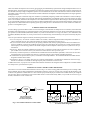
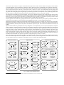
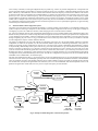
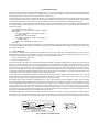
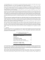
Only the variables used by the task are kept up-to-date in the local table. No synchronization is needed to access this table, since only a
single task has access to it. At the beginning of every cycle of a task, the variables which are input ports are transferred into the local table
from the global table. At the end of the task’s cycle, variables which are output ports are copied from the local table into the global table.
This design ensures that data is always transferred as a complete set.
When using the global state variable table for inter-module communication, the number of transfers per second3 (Zj) for module Mj can be
calculated as follows:
nj
mj


 ∑ S ( x ij ) + ∑ S ( y ij ) + ∆ 


i=1
i=1
Z j = ------------------------------------------------------------------------Tj
(1)
where nj is the number of input ports for Mj, mj is the number of output ports for Mj, xij is input variable xi for Mj, yij is output variable yi
for Mj, S(x) is the transfer size of variable x, Tj is the period of Mj, and ∆ is the overhead required for locking and releasing the state variable
table during each cycle.
We assume that the entire global state variable has a single lock. It is possible for each variable to have its own lock, in which case the
locking overhead increases to (m+n)∆. The advantage of using a single lock is described in Section .A..
The bus utilization B for k modules in a particular configuration, in transfers per second, is then
k
B =
∑ Zj
(2)
j=1
Thus using our state variable table design, we can accurately determine the CPU and bus utilization required for the inter-module communication within a configuration.
A configuration is legal if the following holds true:
 k, m j
   k, n j
  k, m j

 ∩ y ij = ∅  ∧   ∪ x ij  ⊆  ∪ y ij  
 j = 1, i = 1
   j = 1, i = 1   j = 1, i = 1  
(3)
The first term represents the intersection of all output variables from all modules. If two modules have the same outputs, then a join connector is required. Modules with conflicting outputs can modify their output port variables, such that they are two separate, intermediate
variables. A join connector is a separate module which performs some kind of combining operation, such as a weighted average. Its input
ports are the intermediate variables, while its single output port is the output variable that was originally in conflict. The bandwidth required
can then be calculated by treating the join connector as a regular module. Split connectors are not required in our design, since multiple
tasks can specify the same input port, in which case data is obtained from the same location within the global state variable table. The second
term in (3) states that for every input port, there must be a module with a corresponding output port.
Using state variables for module integration is processor independent. Whether multiple modules run on the same RTPU, or each module
runs on a separate RTPU, the maximum bus bandwidth required for a particular configuration remains constant, as computed in (2). In the
next section we give more details on typical modules within a reconfigurable sensor-based control system.
A. Control Module Library
The state variable table mechanism is a means of integrating control modules, which have been developed with a reusable and reconfigurable interface. Once a module is developed, it can be placed into a library, and incorporated into a user’s application as needed. A sample
control module library is shown in Fig. 3. The classification of different module types is for convenience only. There is no difference in the
interfaces of say, a robot interface module and a digital controller module. We expect that existing robot control libraries (e.g. [2][10]), can
be repackaged into reusable modules in order to use them in reconfigurable systems.
The following variable notation is used:
The following subscript notation is used:
d: desired (as input by user or path planner)
θ : joint position
x : Cartesian position
r: reference (computed value, commanded on each cycle)
θ̇ : joint velocity
ẋ : Cartesian velocity
m: measured (obtained from sensors on each cycle)
θ̇˙ : joint acceleration
ẋ˙: Cartesian acceleration
f: Cartesian force/torque
y: wild-card: match any subscript
τ : joint torque
u: control signal
J: Jacobian
z: wild-card: match any variable
Robot interface modules communicate directly with robotic hardware. In general a robot is controlled by sending joint torques to an appropriate input/output port, as represented by the torque-mode robot interface module. The current joint position and joint velocity of the robot
can also be retrieved from the hardware interface. With some robots, direct communication with the robot actuator is not possible. The robot
provides its own controller, to which reference joint positions must be sent. The position-mode robot interface is a module for this type of
3. We use “transfers per second” instead of CPU execution time or bus utilization time as a base measure for the resource requirements of the communication mechanism,
since it is a hardware independent measurement.