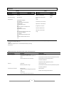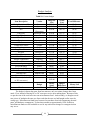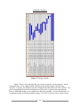
1
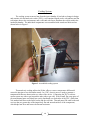
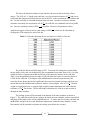
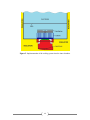
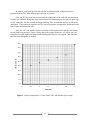
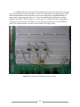
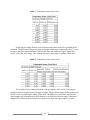
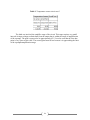
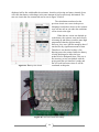
Harding University
MAB-E
(Most Awesome Backpack - Ever)
Midterm Status Report
March 8, 2011
Eric Locke
Natalie Nill Simon Reinhardt Adrian Villalobos
0
Table of Contents
Requirements Specification ……………………………………………………………...……… 2
Project Overview and Status ...................................................................................................…... 9
Sub-Systems
Cooling System ………………………………………………………………..……….. 10
Cooling Chamber ………………………………………………………………….…… 19
DC to DC Converter …………………………………………………………………… 23
Power Control ………………………………………………………………………….. 27
Battery Charger ………………………………………………………………………… 30
Solar Panels …………………………………………………………………………….. 38
Microcontroller ………………………………………………………………………… 45
User Interface …………………………………………………………...……………… 47
Temperature Sensor ………………………………………………….………………… 48
Batteries ………………………………………………………………………………... 52
Full Frame Assembly …………………………………………………………………………... 54
System Integration ……………………………………………………………………………... 54
Budget Analysis ………………………………………………………………………………... 55
Schedule Analysis ……………………………………………………………………………… 56
Appendices
Appendix A: BC547 Transistor Data Sheet …………………………..……….……….. 58
Appendix B: BC557 Transistor Data Sheet ……………………..…………..…...…….. 59
Appendix C: CSD16321Q5 Transistor Data Sheet …………………………...……….. 60
Appendix D: IRF510 NMOSFET Transistor Data Sheet……………………...……….. 61
Appendix E: SCR Rectifier Data Sheet…………...…………………………...……….. 62
Appendix F: Zener Diode Data Sheet ………………………………….……..……….. 63
1
Requirements Specification
Solar Powered Backpack Refrigeration Unit
Adrian Villalobos
Eric Locke
Natalie Nill
Simon Reinhardt
Overview
Vaccines have been one of the most beneficial healthcare discoveries of the past couple
centuries. Unfortunately, many people are unable to receive vaccines because, among other
reasons, health services are unable to reach them while keeping the vaccines cool enough.
According to the PATH organization, transporting vaccines in Africa can be extremely
challenging because regulating the temperatures of vaccines, while transporting them to rural
areas, is difficult and especially challenging in areas without constant power sources1. In 2002,
over 84,000 people died from Hepatitis B (a vaccine that requires cooling) alone2. Some of these
deaths are due to the inability of health organizations to transport vaccines to every place they
are needed. Many of these organizations are working to raise awareness about this issue and find
ways to reach more people. If more people could be reached, thousands of lives could be saved.
There are multiple ways of using alternate power to refrigerate vaccines currently being
used. The most predominant include nonelectric/uncontrolled cold packs, kerosene powered
refrigeration, and solar power. The cold packs have limited use because they have a maximum
cooling time of 48 hours. The kerosene refrigeration is impractical because it requires
continuous refueling and is potentially dangerous. Therefore, our team has decided to use solar
power because it is a portable, reliable, and an efficient way to solve this problem.
Problem Statement
There is a need for a better method for transferring vaccines into rural areas of
developing nations where power is not easily accessible for refrigeration. There is no developed
method that involves continuous refrigeration from a portable, consistent, and environmentally
friendly power source. By having a refrigeration system that can be powered during
transportation, the ability to distribute vaccines will be greatly increased and the chances of
ruining vaccines will be diminished.
Operational Description:
Before Transportation:
Before using the refrigeration backpack to transport vaccines any distance, the target
temperature must be met inside the refrigeration chamber. This can be achieved by one of four
ways:
1
"PATH: Cold Chain." PATH: A Catalyst for Global Health. May 2010. Web. 13 Sept. 2010.
<http://www.path.org/projects/cold-chain.php>.
2
"Statistics about Hepatitis B - WrongDiagnosis.com." Wrong Diagnosis. Aug. 2010. Web. 20 Sept. 2010.
<http://www.wrongdiagnosis.com/h/hepatitis_b/stats.htm>.
2
1. External Power: The pack can be cooled by using external power from any outlet that
has an output standard to the US or African power grid.
2. Cooling Packs: The backpack can be cooled by placing cold packs, such as those used to
keep non-electric vaccine shipping boxes cool, inside the chamber.
3. Refrigerator: The backpack can be cooled by placing the chamber inside a larger
refrigerator or freezer until the target temperature is reached.
4. Solar Power: The backpack can be cooled beforehand using solar power. This method
may require time to charge the packs batteries and cool the chamber.
Also, the batteries must be charged before the vaccines are transported any distance. This
can be accomplished by either using an external power source and/or using solar power to charge
the batteries. For a faster charge time, the batteries can be charged while the cooling system is
off to send all power from the solar panels or external source to the batteries.
The user will be able to select the allowable temperature range via the user interface. First
select the mode for temperature selection, then type in the lowest allowable temperature and then
the highest allowable temperature in that order when prompted on the screen.
During Transportation:
IMPORTANT- Avoid opening the refrigerator door until the destination has been
reached as this will compromise the environment of the vaccines and might deplete the
backpacks energy supply prematurely.
The user will be able to monitor the current temperature inside the refrigerator via the
indicator mounted on the outside of the refrigeration chamber. They will also be able to read the
approximate battery life reading that will inform them as to the amount of energy currently in the
pack in the same screen.
The user should make sure that the solar panels are clear of anything that may block them
from the sun when possible.
After Transportation:
When the destination is reached the user should transfer the vaccines to a secure
environment to be used as needed. The backpack should remain in the refrigeration mode until
vaccines are no longer stored in the chamber.
Technical Requirements
· The unit will cool a chamber within the backpack and maintain it at a temperature range
between 2℃ and 8℃ (35℉ and 46℉ ), for a minimum of 48 hours, at an average ambient
temperature up to 30°C (86°F), while stationary.
· The temperature inside the refrigeration chamber will be read and relayed so it can be
displayed on the outside of the unit. The temperature sensor will have a maximum
resolution range of ± 1℃ , and will cover a temperature range of at least 0°C to 30°C
(32°F to 86°F).
3
·
·
·
·
·
·
·
·
The entire unit will weigh less than 37 kg (≈ 82 lbs).
The backpack will not exceed a size of 60 cm x 100 cm x 60 cm.
The refrigeration system will be controlled to within the specified temperature range.
The unit will be able to measure the temperature inside the chamber to within ± 1℃ .
The unit will be able to control the temperature inside the chamber to within± 3℃ .
There will be a user interface used to control the refrigeration system. It will include: an
on/off switch, a digital temperature display, a temperature control interface, and battery
status indicators.
The unit will have a frame that can perform while being transported on foot and by
vehicle.
All systems will operate in a safe manner that will pose no threat of harm to the users.
Temperatures will not go above 50°C or below -30°C, voltages will not exceed 30 V DC,
and moving parts will be protected by a grill.
Deliverables
1. User’s Manual
2. Technical Drawings and Analysis of Hardware
3. Schematic of Circuit with Simulation Results
4. Code and Flowcharts
5. Report of Testing
6. Parts List with Budget
7. Final Technical Report
8. Solar Powered Refrigeration Backpack
Preliminary Test Plan
· Four healthy individuals, with a minimum height of 1.6 m (≈ 63 inches) and weight of 54 kg
(≈ 120 lbs), will be able to pick up, put on, and take off the backpack with the assistance of
one other individual.
· A performance test will be conducted. The backpack will be taken on a mile hike then will
immediately be put into a ventilation chamber for a 48 hour period. It will be tested at
temperatures between 22°C and 30°C (≈ 72°F and 86°F). The solar panels will be exposed
to two cycles of simulated sunlight for 12 hours then darkness for 12 hours. The maximum
and minimum temperatures will be recorded over that period. This test will be executed
three times.
· Temperature gauge will be tested to insure accurate (within ± 1°C) temperature readings
inside the chamber.
· Backpack will be weighed to ensure it does not exceed the maximum weight.
4
Attachments
The following attachments come from the site:
“Centers for Disease Control and Prevention.” Web. 13 Sept 2010.
Guidelines for Maintaining and Managing the Vaccine Cold Chain
In February 2002, the Advisory Committee on Immunization Practices (ACIP) and American
Academy of Family Physicians (AAFP) released their revised General Recommendations on
Immunization (1), which included recommendations on the storage and handling of
immunobiologics. Because of increased concern over the potential for errors with the vaccine
cold chain (i.e., maintaining proper vaccine temperatures during storage and handling to preserve
potency), this notice advises vaccine providers of the importance of proper cold chain
management practices. This report describes proper storage units and storage temperatures,
outlines appropriate temperature-monitoring practices, and recommends steps for evaluating a
temperature-monitoring program. The success of efforts against vaccine-preventable diseases is
attributable in part to proper storage and handling of vaccines. Exposure of vaccines to
temperatures outside the recommended ranges can affect potency adversely, thereby reducing
protection from vaccine-preventable diseases (1). Good practices to maintain proper vaccine
storage and handling can ensure that the full benefit of immunization is realized.
Recommended Storage Temperatures
The majority of commonly recommended vaccines require storage temperatures of 35°F--46°F
(2°C--8°C) and must not be exposed to freezing temperatures. Introduction of varicella vaccine
in 1995 and of live attenuated influenza vaccine (LAIV) more recently increased the complexity
of vaccine storage. Both varicella vaccine and LAIV must be stored in a continuously frozen
state <5°F (-15°C) with no freeze-thaw cycles (Table 1). In recent years, instances of improper
vaccine storage have been reported. An estimated 17%--37% of providers expose vaccines to
improper storage temperatures, and refrigerator temperatures are more commonly kept too cold
than too warm (2, 3).
Freezing temperatures can irreversibly reduce the potency of vaccines required to be stored at
35°F--46°F (2°C--8°C). Certain freeze-sensitive vaccines contain an aluminum adjuvant that
precipitates when exposed to freezing temperatures. This results in loss of the adjuvant effect and
vaccine potency (4). Physical changes are not always apparent after exposure to freezing
temperatures and visible signs of freezing are not necessary to result in a decrease in vaccine
potency.
Although the potency of the majority of vaccines can be affected adversely by storage
temperatures that are too warm, these effects are usually more gradual, predictable, and smaller
in magnitude than losses from temperatures that are too cold. In contrast, varicella vaccine and
LAIV are required to be stored in continuously frozen states and lose potency when stored above
the recommended temperature range.
5
Vaccine Storage Requirements
Vaccine storage units must be selected carefully and used properly. A combination
refrigerator/freezer unit sold for home use is acceptable for vaccine storage if the refrigerator and
freezer compartments each have a separate door. However, vaccines should not be stored near
the cold air outlet from the freezer to the refrigerator. Many combination units cool the
refrigerator compartment by using air from the freezer compartment. In these units, the freezer
thermostat controls freezer temperature while the refrigerator thermostat controls the volume of
freezer temperature air entering the refrigerator. This can result in different temperature zones
within the refrigerator.
Refrigerators without freezers and stand-alone freezers usually perform better at maintaining the
precise temperatures required for vaccine storage, and such single-purpose units sold for home
use are less expensive alternatives to medical specialty equipment. Any refrigerator or freezer
used for vaccine storage must maintain the required temperature range year-round, be large
enough to hold the year's largest inventory, and be dedicated to storage of biologics (i.e., food or
beverages should not be stored in vaccine storage units). In addition, vaccines should be stored
centrally in the refrigerator or freezer, not in the door or on the bottom of the storage unit, and
sufficiently away from walls to allow air to circulate.
Temperature Monitoring
Proper temperature monitoring is key to proper cold chain management. Thermometers should
be placed in a central location in the storage unit, adjacent to the vaccine. Temperatures should
be read and documented twice each day, once when the office or clinic opens and once at the end
of the day. Temperature logs should be kept on file for >3 years, unless state statutes or rules
require a longer period. Immediate action must be taken to correct storage temperatures that are
outside the recommended ranges. Mishandled vaccines should not be administered.
One person should be assigned primary responsibility for maintaining temperature logs, along
with one backup person. Temperature logs should be reviewed by the backup person at least
weekly. All staff members working with vaccines should be familiar with proper temperature
monitoring.
Different types of thermometers can be used, including standard fluid-filled, min-max, and
continuous chart recorder thermometers (Table 2). Standard fluid-filled thermometers are the
simplest and least expensive products, but some models might perform poorly. Product
temperature thermometers (i.e., those encased in biosafe liquids) might reflect vaccine
temperature more accurately. Min-max thermometers monitor the temperature range. Continuous
chart recorder thermometers monitor temperature range and duration and can be recalibrated at
specified intervals. All thermometers used for monitoring vaccine storage temperatures should be
calibrated and certified by an appropriate agency (e.g., National Institute of Standards and
Technology). In addition, temperature indicators (e.g., Freeze Watch™ [3M, St. Paul, Minnesota]
or ColdMark™ [Cold Ice, Inc., Oakland, California]) can be considered as a backup monitoring
system (5); however, such indicators should not be used as a substitute for twice daily
temperature readings and documentation.
6
All medical care providers who administer vaccines should evaluate their cold chain
maintenance and management to ensure that 1) designated personnel and backup personnel have
written duties and are trained in vaccine storage and handling; 2) accurate thermometers are
placed properly in all vaccine storage units and any limitations of the storage system are fully
known; 3) vaccines are placed properly within the refrigerator or freezer in which proper
temperatures are maintained; 4) temperature logs are reviewed for completeness and any
deviations from recommended temperature ranges; 5) any out-of-range temperatures prompt
immediate action to fix the problem, with results of these actions documented; 6) any vaccines
exposed to out-of-range temperatures are marked "do not use" and isolated physically; 7) when a
problem is discovered, the exposed vaccine is maintained at proper temperatures while state or
local health departments, or the vaccine manufacturers, are contacted for guidance; and 8)
written emergency retrieval and storage procedures are in place in case of equipment failures or
power outages. Around-the-clock monitoring systems might be considered to alert staff to afterhours emergencies, particularly if large vaccine inventories are maintained.
Additional information on vaccine storage and handling is available from the Immunization
Action Coalition at http://www.immunize.org/izpractices/index.htm. Links to state and local
health departments are available at http://www.cdc.gov/other.htm. Especially detailed guidelines
from the Commonwealth of Australia on vaccine storage and handling, vaccine storage units,
temperature monitoring, and stability of vaccines at different temperatures (6) are available at
http://immunise.health.gov.au/cool.pdf.
References
1. CDC. General recommendations on immunization: recommendations of the Advisory
Committee on Immunization Practices (ACIP) and the American Academy of Family
Physicians (AAFP). MMWR 2002;51(No. RR-2).
2. Gazmararian JA, Oster NV, Green DC, et al. Vaccine storage practices in primary care
physician offices. Am J Prev Med 2002;23:246--53.
3. Bell KN, Hogue CJ, Manning C, Kendal AP. Risk factors for improper vaccine storage
and handling in private provider offices. Pediatrics 2001;107:E100.
4. World Health Organization. Thermostability of vaccines. Geneva, Switzerland: World
Health Organization, 1998; publication no. WHO/GPV/98.07. Available at
http://www.who.int/vaccines-documents/DocsPDF/www9661.pdf.
5. World Health Organization. Temperature monitors for vaccines and the cold chain.
Geneva, Switzerland: World Health Organization, 1999; publication no.
WHO/V&B/99.15. Available at http://www.who.int/vaccinesdocuments/DocsPDF/www9804.pdf.
6. Commonwealth Department of Health and Aged Care. Keep it cool: the vaccine cold
chain. Guidelines for immunisation providers on maintaining the cold chain, 2nd ed.
Canberra, Australia: Commonwealth of Australia, 2001.
7
TABLE 1. Vaccine storage temperature
requirements
35°F-46°F
(2°C-8°C)
≤5°F
(-15°C)
Instructions
Vaccine
Do not freeze or
Diphteria-, tetanus, or pertussis-containning
vaccines
Instructions
Instructions
expose the freezing
(DT, DTaP, Td)
Maintain in continuosly
frozen state with no freezethaw
cycles.
temperatures.
Haemophilus conjugate
vaccine (Hib)*
Hepatitis A (HepA) and hepatitis B
(HepB) vaccines
Inactivated polio vaccine
(IPV)
Measles, mumps, and rubella vaccine
(MMR) in the
lyophilized (freeze-dried)
state†
Vaccine
Live attenuated
influenza
vaccine
(LAIV)
Contact state or local health
department or manufacturer
for guidance on vaccines
exposed to temperatures
above the recommended
Meningoccoccal polysaccharide vaccine
Pneumococcal conjugate
vaccine (PVC)
Pneumococcal polysaccharide vaccine
(PPV)
Trivalent inactivated inflenza vaccine
(TIV)
range.
*ActHIB® (Aventis Pasteur, Lyon, France) in the lyophilized state is not expected to be affected detrimentally by freezing
temperatures, although nodata are
available.
†MMR in the lyophilized state is not affected detrimentally by freezing
temperatures.
TABLE 2. Comparison of thermometers used to monitor avccine temperatures
Thermometer type
Advantages
Disadvantages
Standard fluid-filled
Inexpensive and simple to use.
Thermometers encased in biosafe liquids can
reflect
Less accurate (+/-1°C).
vaccine temperatures more accurately.
No information on min/max temperatures.
No information on duration of out of specification exposure.
Cannot be recalibrated.
Inexpensive models might perform poorly.
Min-max
inexpensive
Less accurate (+/-1°C).
Monitors temperature range.
No information on duration of out of specification exposure.
Cannot be recalibrated.
Continuous chart recorder
Most accurate
Continuous 24-hour readings of temperature
range
and duration.
Can be recalibrated at regular intervals.
8
Most expensive.
Requires most training and maintenance.
Project Overview and Status
There is a need for a better method for transferring vaccines into rural areas of
developing nations where power is not easily accessible for refrigeration. There is no developed
method that involves continuous refrigeration from a portable, consistent, and environmentally
friendly power source. By having a refrigeration system that can be powered during
transportation, the ability to distribute vaccines will be greatly increased and the chances of
ruining vaccines will be diminished.
Our goal is to create a means of transporting vaccines to remote areas in rural parts of
developing countries. The design is a solar powered backpack refrigerator. The device will be
driven by a battery which can be recharged by either plugging it into a 110 V AC power outlet or
12 V DC car jack when available, or by a solar panel that is attached to the backpack when on
foot. A user interface will allow the user to set the temperature within the insulated chamber and
will inform him of the current temperature. It will also warn the user if the temperature ever gets
too high so that the ruining of vaccines can be prevented. A microcontroller continuously checks
the temperature within the insulated chamber and decides whether it needs to be cooled. The
device will weigh less than 37 kg (≈ 82 lbs) and will not exceed a size of 60 cm x 100 cm x 60
cm.
The major accomplishments that have been reached this semester include constructing
the inner chamber of the backpack, conducting performance tests on the cooling system, solar
panels and batteries, integrating the cooling system into the insulation and inner chamber,
building the insulation around the inner chamber, constructing the temperature sensor circuit,
assembling the user interface circuit, and making a detailed circuit image to be sent to a
professional company to be etched.
Though we have reached many of our goals on time, we are still slightly behind schedule
in coding the microprocessor and constructing peripheral circuitry and building the cooling
chamber.
Over the next few weeks we plan to complete tests on the solar panels and batteries to
obtain detailed measurements on the output of each under different operating conditions. We
will also develop code to use the analog to digital system of the microcontroller, finish testing
the cooling system and insert it into the chamber, and begin constructing and soldering the DC to
DC converter.
9
Cooling System
The cooling system removes heat from the inner chamber. It has had no change in design
and consists of a thermoelectric cooler (TEC), a self contained liquid cooler with radiator and fan
to dissipate heat to the environment, and a cold sink with fan to distribute the cold air within the
insulated chamber. The individual components were assembled with round steel bolts and are
shown below in Figure 1.
Figure 1: Assembled cooling system
Thermoelectric cooling utilizes the Peltier effect to create a temperature differential
across the junction of two dissimilar metals. In a TEC, electric power is used to generate a
temperature difference between the two sides of the device. Connecting the TEC to a direct
current causes one side to get hot and the other side to get cold. With a small, flat scrap piece of
plywood thermal paste was thinly but evenly distributed over both sides of the TEC, which then
was sandwiched between the liquid cooler and the cold sink. Thermal paste fills small voids and
crevices that are present due to the imperfectly flat and smooth surfaces of the components,
which helps heat flow and lowers the thermal resistance.
10
The lower the thermal resistance a heat sink has, the more it allows the flow of heat
℃
energy. The ECO A.L.C. liquid cooler unit has a very low thermal resistance (0.1 ) and acts as
a heat sink that dissipates heat from the hot side of the TEC to the environment via a radiator and
fan. For the cold sink, an extruded aluminum sink was used. In order to reduce the thermal
℃
resistance and satisfy the requirement of 0.916 , the cold sink was combined with a low profile
fan. Fans are commonly rated in CFM (
) of airflow. However, the parameter used to
calculate the impact of forced air on a sink rating is LFM (
dividing the CFM rating by the area of the fan.
) which can be calculated by
Table 1: Cold sink adjustment factor as a function of airflow of the fan
The cold side fan has an LFM rating of 476. To account for backpressure which limits
the net airflow, this value was multiplied by the recommended correction factor of 0.8. In order
to find the factor of improvement that the fan has on the thermal resistance of the cold sink,
Table 1 was interpolated between the values of 300 and 400 which gives a correction factor of
0.3896 for the cold sink. Dividing the cold sink’s thermal resistance requirement by this
correction factor shows that the fan significantly decreases the thermal resistance which in turn
℃
means that the cold sink’s thermal resistance can have a much higher value of 2.35 . Because
weight is a big design factor, a compact, light weight extruded aluminum sink with a thermal
℃
resistance of 2.0 was chosen. The fan also helps to distribute the cold air to and circulate it
through the inner chamber.
The cooling system will be attached to the bottom of the inner chamber as shown in
Figure 2. The cold sink and the fan are going to be inside the inner chamber, and the water block
and pump of the liquid cooler will be attached below it. To ensure that no vaccines can block the
fan’s airflow and prevent an evenly distributed temperature within the inner chamber, a mesh
like material will be installed to separate the cooling system from the vaccines.
11
Figure 2: Implementation of the cooling system into the inner chamber
12
In order to verify that the cold sink and fan are indeed needed, multiple tests were
performed on the TEC with different parts missing in each test.
First, the TEC by itself was powered and the temperature of the cold side was measured.
No data was collected during this experiment because the temperature on the cold side spiked up
to 32℃ within the first few seconds and kept climbing. This verified that the TEC could not be
used alone. This result was expected; the TEC can only generate a temperature differential if the
heat is removed from its hot side.
Next, the TEC was attached to the water block of the liquid cooler, and only the fan but
not the pump was powered. Figure 3 below shows the results of this test. As can be seen, the
temperature cooled slightly but then started climbing until the test was stopped. This indicates
that more heat dissipation is needed.
45.0
40.0
35.0
Temperature (℃ )
30.0
25.0
20.0
15.0
10.0
5.0
0.0
0
0.5
1
1.5
2
2.5
Time (min)
Figure 3: Graph of temperature vs. time for the TEC and radiator (fan on only)
13
3
Temperature (℃ )
After this, the TEC was left attached to the radiator while only the pump of the liquid
cooler was powered. Figure 4 shows the results of this test. As can be seen, the temperature
decreased, but then slowly increased until the test was stopped. This indicates that more heat
dissipation is needed.
23.0
22.0
21.0
20.0
19.0
18.0
17.0
16.0
15.0
14.0
13.0
12.0
11.0
10.0
9.0
8.0
7.0
6.0
5.0
4.0
3.0
2.0
1.0
0.0
0
1
2
3
4
5
6
7
8
9
Time (min)
Figure 4: Graph of temperature vs. time for the TEC and radiator (pump on only)
14
10
Temperature (℃ )
Next, the TEC was left attached to the water block and the entire liquid cooler with its
pump and fan were powered. Figure 5 shows the results of this test at two different ambient
temperatures of 22.5℃ (Series 1) and 29.4℃ (Series 2). As can be seen, the temperature
decreased to an average of 5℃ and 8℃ respectively, but this is not low enough for our
requirement specification. Thus, more heat dissipation is needed.
30.0
29.0
28.0
27.0
26.0
25.0
24.0
23.0
22.0
21.0
20.0
19.0
18.0
17.0
16.0
15.0
14.0
13.0
12.0
11.0
10.0
9.0
8.0
7.0
6.0
5.0
4.0
3.0
2.0
1.0
0.0
Series1
Series2
0
1
2
3
4
5
6
7
8
9
Time (min)
Figure 5: Graph of temperature vs. time for the TEC and liquid cooler
15
10
Temperature (℃ )
A test was run with the TEC just connected to the cold sink in order to see if liquid cooler
was needed with the cold sink. Figure 6 shows the results from this test. As can be seen, the
TEC did not cool down at all since no heat was being dissipated. This verifies that the liquid
cooler is needed with the cold sink.
24.0
23.0
22.0
21.0
20.0
19.0
18.0
17.0
16.0
15.0
14.0
13.0
12.0
11.0
10.0
9.0
8.0
7.0
6.0
5.0
4.0
3.0
2.0
1.0
0.0
0
0.5
1
1.5
2
2.5
3
3.5
4
4.5
5
Time (min)
Figure 6: Graph of temperature vs. time for the TEC and cold sink
Once it was confirmed that both the radiator and the cold sink were needed, several test
runs at two ambient temperatures were performed to ensure functioning of the cooling system.
Because the cold sink was surrounded by warm air, the cold side fan was not turned on in these
test runs. Conduction from the ambient air to the cold sink would have prohibited accurate
results, because it would have prevented the cold sink from cooling below freezing if warm air
was blown across its fins. The temperature of the cold sink was measured with an infrared
temperature gauge. All components were supplied with 12 V DC and both the current and
temperature were recorded with respect to time. Table 2, on the following page, shows the cold
sink temperature at ambient temperatures of 22.5℃ and 29.4℃ and the associated current draw.
The temperature of the reservoir of the liquid cooler never got higher than 5℃ above the ambient
temperature. Figure 7 gives a better understanding of the time frame at which the cooling took
place.
16
Table 2: Data from cooling system tests
Test @ 22.5℃ (Series 1)
Temperature
Current
(℃ )
(A)
22.5
3.40
22.0
3.19
19.3
3.15
13.9
3.13
8.9
3.10
4.4
3.09
0.6
3.08
-1.9
3.07
-4.1
3.05
-5.3
3.04
-6.8
3.04
-7.6
3.04
-8.4
3.03
-9.1
3.03
-9.6
3.03
-10.0
3.02
-10.0
3.02
-10.0
3.02
Time
(min)
0
1
2
3
4
5
6
7
8
9
10
11
12
13
14
15
16
17
Test @ 29.4℃ (Series 2)
Temperature
Current
(℃ )
(A)
29.4
3.42
28.7
3.23
24.3
3.19
18.1
3.14
13.2
3.11
7.2
3.1
1.5
3.08
-0.6
3.07
-2.6
3.05
-4.8
3.04
-6.2
3.04
-7.0
3.04
-7.8
3.03
-8.4
3.03
-9.1
3.03
-9.3
3.03
-9.3
3.03
-9.3
3.02
30.0
25.0
Temperature (℃ )
20.0
15.0
10.0
Series1
5.0
Series2
0.0
-5.0
-10.0
0
1
2
3
4
5
6
7
8
9
10 11 12 13 14 15 16 17
Time (min)
Figure 7: Graph of temperature vs. time for cooling system tests
17
Because the voltage is constant, it can be concluded that the resistance of the TEC
decreases with a decrease in temperature. When the cooling system is initially turned on, the
current spikes but quickly decreases and eventually levels out around 3 A. Both the fan and the
pump took a current of 0.11 A each which means that the TEC took the rest of the current which
was 2.78 A, which is a value very close to the expected value of 2.82 A.
The design assumed the cooling system to reach the operating temperature range of 2℃
to 8℃ instantaneously. This test shows that this range is not reached until approximately five
minutes after the cooling system is turned on. This could potentially cause an imbalance to the
power management. However, both fans and the pump of the liquid cooler use less current than
expected (see Table 3). One way to conserve energy would be to not turn on the cold side fan
until the operating temperature range is reached, which would save an additional 0.24 A for that
time.
Table 3: Expected vs. actual current draw for components of cooling system
Component Expected Current (A) Actual Current(A)
TEC
2.82
2.78
Cold Side Fan
0.3
0.24
Radiator Fan
0.3
0.11
Pump
0.14
0.11
Total
3.56
3.24
On average, the cooling system used 37 W of power. If the cold side fan was used, the
power would increase to a value of 40 W.
18
Cooling Chamber
There are three main parts that make up the cooling chamber: 1) the inner chamber, 2)
insulation, and 3) the outer chamber. The plan is to build outwards. This avoids several
problems and ensures it all fits together well. Figure 8 below shows how the three parts will fit
together.
Inner Chamber
Chamber depth = 20cm
Total depth = 47cm
Outer Chamber
Chamber width = 30cm
Insulation
Total width = 57cm
Figure 8: Top view of cooling chamber
The inner chamber has been completed (the lid is not attached since it will be attached to
the outer chamber lid) and can be seen in Figure 10. The wall material used is the tempered
hardboard that was chosen last semester and the screws are countersink screws. The inner
chamber is very sturdy. No specific test was performed because it is not very important for the
inner chamber to be sturdy since it will be surrounded by rigid insulation and an outer chamber.
But once completed it was shaken and shown to be rigid and unmoving. The cooling system has
been attached to the bottom of the inner chamber as mentioned in the previous section and
illustrated in Figure 2. To seal the inner chamber and prevent moisture from seeping into the
insulation, the inner corners and the bottom of the cold sink were sealed with white caulking
(shown in Figure 9).
19
Figure 9: Inside view of the inner chamber after caulking
Height
Width
Depth
Figure 10: Inner chamber
Width = 57cm, Depth = 47cm, Height = 75cm
20
Rigid Styrofoam insulation will be used to significantly decrease the rate at which heat
enters the inner chamber of the backpack. A total of five layers of the 2.54 cm (1 inch) thick
insulation will surround each side of the chamber. With a box cutter, the insulation was cut to
the correct dimensions. In order to increase the stiffness, the first layer of the insulation was
pressed onto the screws of the brackets that hold the inner chamber together (shown in Figure
11).
Figure 11: Insulation shell built on top of inner chamber
The next layers were attached to the first layer using wood glue. Clamps were used to
press the layers together while the glue was drying. Four layers of the insulation have been
completed. The rest of the build will be completed by the end of the first week after spring
break. This can be seen in Figure 11. The insulation is being built around the box in a puzzle fit,
as illustrated in Figure 12 (not to scale). This allows for a close fit that minimizes air pockets
(which increase heat loss). The cooling system has been integrated into the insulation and has
been built so that it can be removed in case any unforeseen complications occur.
21
Inner chamber
Side view (top)
Side view (bottom)
Bird's eye view
Figure 12: Insulation placement
The outer chamber has not been built yet and will not be built until the insulation has
been built around the inner chamber and has all the components integrated into it. The outer
chamber is a simple build and will not take long. It will be tested as is described in the
requirements specification.
22
DC to DC Converter
The DC to DC converter circuits were modified since it was decided to change the inputs
from 12V to 6V. This modification has to be done because we found easier to use op-amps. The
op-amps comprise the amplification necessary to create an output from the sensor circuit that
moves across the full range of the microcontroller’s A/D converter system.
The cooling system will be powered with 12V being supplied from the batteries, and op
amps will be used to derive the steady 6V needed for the microprocessor, temperature sensor,
and user interface. These 6V coming from the voltage regulator will power the DC to DC
converters. The same buck converter integrated circuits (TPS40192) are still going to be used for
the DC to DC converters of the microprocessor and temperature sensor, which operate with 3.3V
and 3.0 respectively. A DC to DC converter circuit for the user interface cannot be created with
the IC TPS40192 because in order to provide an output of 5V, the buck converter would require
a duty cycle greater than 85% which cannot be operated by the IC TPS40192. In order to power
the user interface, a regular 5V voltage regulator will be used. Although regular voltage
regulators are usually not recommended because of their inefficiencies, we have decided to use
one in this case because the drop out voltage is going to be very small (1V) and it will not
produce that much heat. Figure 13 shows how the DC to DC converters will power the
microprocessor, temperature sensor and user interface, while the cooling system will be directly
powered from the batteries.
Figure 13: The DC to DC converters have been modified so that their input is 6V instead of 12V
The good thing about the structure of the circuits that use the integrated circuit TPS40192
is that in order to modify the output voltage only the values of the capacitors and resistors
change. The new DC to DC converters operate with V
= 5.8V and V
= 6.2V. The electric
components in order to build the previous designs were already ordered and received. Although
modifications have been made, the same buck converters and buck transistors are going to still
23
be used. Only capacitors with new values need to be ordered. The modified circuits are shown
next.
Figure 14: New circuit design of DC to DC converter for the microprocessor
V ,
5.8V, V ,
6.2V, V
3.30V, I
0.05A
Figure 15: New circuit design of DC to DC converter for temperature sensor
V ,
5.8V, V ,
6.2V, V
3.00V, I
0.01A
24
Before the last modifications were made, we started working with the printed circuit
board. But a problem we have been facing is that the footprints for the integrated circuits have
not been found. These ICs manufactured by Texas Instruments are so small the circuit board
needs to be precisely made in order to have a successful soldering. We have been trying to
contact this company in order to get the footprints of the TPS40192 (buck converter) and
CSD16321Q5 (NFET transistor). Since these footprints are unavailable, we are currently
drawing them using software given the size specifications. We have considered that these printed
circuit boards should be professionally made due to the high precision it is required.
Figure 16: TPS40192 IC size specifications and shape
25
Figure 17: Several footprints have been tested in order to see which one is the
best match to the integrated circuit
26
Power Control
The power control has been designed, built in a breadboard and tested. The circuit has an
N channel power MOSFET transistor IRF510 that works as a switch. The gate pin of the
transistor will be connected to one of the outputs of the microprocessor, and this will send a
digital signal (0 or +5V). The source pin of the transistor is connected to the circuit ground. The
negative side of the load (fan, cooler and TEC) is connected to the drain of the transistor, and the
positive side is connected to the positive terminal of the external power supply (12V lead acid
battery). Now, whether the transistor is on or off will depend on whether the gate is at 0V or 5V.
When the gate is at 0 V, the transistor stays off, so no current can flow keeping the cooling
system off. But when the gate is at 5V, the transistor turns on and it starts acting as a very low
resistance current path, so current can flow. The current will flow from the battery to the load
into the drain of the transistor and then out from the source of the transistor into ground. So when
the transistor is on, the cooling system will turn on too. Figure 18 shows the circuit built in the
breadboard using an LED to test its functionality. When gate is connected to 5V the LED turns
on, and remains on until it is connected to ground (0V.)
Figure 18: Power control circuit
27
Figure 19: Testing the power control circuit with an LED. The LED turns on and off depending
on whether the gate of the transistor is at 5V or 0V.
The circuit was tested with an LED to show its right functioning, and later it was
connected to the cooling system. But before the power control circuit was connected, the cooling
system was connected to the 12V power supply and it draw a current of 2.095A when it was
expected to draw about 3.5A. The cooling system was working and cooling but it seemed there
might had been a problem with the power supply or the TEC (which is the component that draws
most of the current).
The power control circuit was then connected to the cooling system as shown in Figure
20 and tested. When the gate pin of the transformer was connected to ground (simulating the 0V
digital signal) the cooling system was off. When the pin was connected to a 5V the cooling
system would turn on, and remain on until it was connected again to ground. The transistor
increased in temperature when it was on, so a heat sink had to be added. The current draw from
the power supply was kept to 2.095A, the same as when the cooling system was tested directly
with the power source. These results showed that the power control was working correctly and
the microprocessor will be able to turn the cooling system on and off.
28
Figure 20: Testing the power control circuit with the cooling system.
A 5V voltage at the gate of the transistor turns the cooling system on.
29
Battery Charger
After looking at different options for circuit designs it was decided to use a circuit that
uses a 12V transformer. The circuit is shown in Figure 21. The circuit was originally taken from
the website talkingelectronics.com, but some modifications were made on our design.
Figure 21: Battery charger circuit
The circuit does not turn on until a battery is connected across the terminals as shown in
the diagram. This action turns on the PNP transistor in the Turn ON block (shown in Figure 22).
The resistance between the collector-emitter terminals decreases and the indicator LED comes
on. The path to the bottom rail of the circuit goes through a signal diode, the gate-cathode
junction of the SCR (Silicon Controlled Rectifier) and through three 3.9 Ω resistors in parallel.
This is why the LED illuminates. The circuit works on an AC plug pack. A DC supply will not
allow the SCR to turn off, as it turns off when the current through it falls to zero.
The circuit is a half-way rectifier so it only charges the battery on every half cycle. The
plug pack does not like this as it leaves residual flux in the core of the transformer and causes it
to get warm. But that is the only disadvantage of the circuit.
30
The SCR turns on during each half cycle and current flows into the battery. A voltage is
developed across three 3.9 Ω resistors (in parallel) and this voltage is fed into the 47uF capacitor.
It charges and turns on the BC547 transistor located in the Maximum Current block. The
transistor robs the SCR of gate voltage and the SCR turns off. The energy in the 47uF capacitor
feeds into the transistor but after a short time it cannot keep the transistor turned on.
The transistor turns off and the SCR switches on and delivers another pulse of current to the
battery. As the battery charges, its voltage increases and this is monitored by the Voltage
Monitor block.
Figure 22: Functional blocks of the battery charger circuit
31
The circuit is very complex and one way to look at the operation is to consider the top rail
as a fixed rail and as the battery voltage increases, the rail connected to the negative terminal of
the battery is pushed down. This lets you see how the Turn On transistor is activated and how
the Voltage Monitor block components create voltage drops across each of them.
The Voltage Monitor block components consist of a transistor and zener diode as well as an 8.2
KΩ resistor, a 1KΩ potentiometer (or trim pot), a 1.5 KΩ resistor, a 150 Ω resistor and a signal
diode.
The signal diode is actually part of the flasher circuit. As the voltage across the battery
increases to 13.75 volts, each resistor in the voltage detecting block will have a voltage drop
across it that corresponds to the resistance of the resistor. The diode has a constant 0.7V across it.
The voltage on the wiper of the pot will be about 3.25v and the voltage across the zener will be
10V. This leaves 0.6V between the base and emitter of the Voltage Monitor transistor.
This voltage is sufficient to turn the transistor ON. When the Voltage Monitor transistor turns
ON, it robs the "Turn On" transistor of base-emitter voltage and the circuit turns off.
The SCR has only two states: ON and OFF. During the half-cycle when it is turned on,
the battery gets a high pulse of current and the current is only limited by the capability of the
plug pack. There is not enough energy to allow very high pulses of current to be delivered and
this is fortunate as the SCR is only a 0.8 A device, but will endure surges of 10A for half a cycle.
Whenever the SCR is triggered into conduction during the half cycle of its operation, it remains
in conduction until the voltage delivered by the plug pack falls to zero. This is when the SCR
turns off.
When the plug pack delivers a negative voltage to the top rail and a positive voltage to
the lowest rail, the SCR is not triggered into conduction and none of the components in the
circuit deliver current to the battery. The SCR delivers current for a few half-cycles and then it is
turned off for a few cycles. This is how the average current delivered to the battery is controlled.
The circuit is designed to deliver about 180-220 mA average charge-current. The actual value is
determined by the three 3.9 Ω resistors in parallel.
When the battery is fully charged, the indicator LED begins to flash. The flashing is
produced by the 2.2 KΩ resistor and 47uF capacitor connected to the voltage monitor section.
When the battery is charging, the capacitor is charged via the diode connected to the BC557
transistor and through the 150 Ω and signal diode to the negative of the battery. When the battery
is fully charged, the Voltage Monitor section turns ON and turns off the "Turn ON" section. This
removes the voltage on the positive side of the 47Uf capacitor and the positive side is brought to
the negative rail via the 2.2K Ω resistor. This brings down the negative side of the capacitor and
the 150 Ω resistor is allowed to drop below the negative rail due to the presence of the diode, as
the diode becomes reverse-biased. This holds the circuit in the "off" condition, as the voltage
monitor section sees an extra voltage across it and thinks the battery it is "over-charged."
The electric components for this circuit have been ordered and received. The footprint
has already been design using Ultiboard, and the board was etched.
32
Figure 23: Footprint of the battery charger circuit in Ultiboard
Figure 24: 3D view of the battery charger circuit
33
Figure 25: Footprint used for the zener diode
The components were soldered into the board as shown in Figure 26. All the components
were mounted on one side of the board, except for the zener diode, which was surface mounted
on the other side.
.
.
……………
Figure 26: The soldered circuit of the battery charger
34
Once the circuit was complete it was hooked to the power plug and to the 12V battery,
and the circuit was tested. The LED turned on, and the current going into the battery was
measured. The battery was being charged with a current of 20mA, when it was supposed to be of
about 200mA. This current was very small that the voltage of the battery was kept constant with
a value of 12.45V during the testing period of 15 minutes, as shown in Figure 27. The circuit was
carefully analyzed until the problem was found. The output of the power plug was providing 12V
and 500 mA, but the current was DC instead of AC. It must be an AC supply as we do not want
any electrolytics (substance that disassociates into ions and can transmit electric current through
positively and negatively charged ions)to be present on the power rail as this will allow a very
high charge-current to flow and possibly damage the SCR. A DC supply will not allow the SCR
to turn off, as it turns off when the current through it falls to zero. It was decided to keep the DC
power plug, as it will be useful for powering the cooling system when a wall outlet is available
as specified in the requirement specifications.
Figure 27: Testing the circuit: LED is on, current flowing to the battery is 18 mA, and voltage
across the battery (12.45V) remains constant
The correct power plug was ordered and the circuit was tested. The current charging the
battery was of 195mA. The initial voltage of the battery was 12.45V and in five minutes the
voltage increased to 12.50V. This showed that the circuit was actually charging the battery, but it
was considered that another test was required by charging a battery that was almost fully
discharged. So the 12V lead acid battery was discharged by connecting it to the load shown in
Figure 46 for 12 periods of an hour each (to prevent overheat in the resistors) until the voltage
across the battery was dropped to 10.7V. The battery was then connected to the battery charger
circuit for 27 hours and the voltage and current were measured constantly. Figure 29 shows a
35
graph with the voltage of the battery as it is being charged during the test period. From this
figure it can be observed that the voltage of the battery increased at a faster rate in the first 3
hours of testing, while in the next hours the voltage increase rate was smaller but was kept
constant. 27 hours is a long period of time to charge the battery 1.5V, but considering that it is
12AH battery being charged with a 200mA current (small current that is safe for the battery if
kept unattended) makes it a reasonable time. The current that charged the battery was constantly
varying. When the circuit started to charge the battery, a current of 194mA was being supplied to
the battery, then in the next hour it drop to about 182mA, and in the rest of the test of test the
current was varying constantly between 173mA and 177mA.
Figure 28: Charging the battery at 5.5hrs after the test was initiated. The voltage in the battery
has increased 0.95V. The LED is on and the current flowing to battery is 173 mA
36
12.6
12.4
Battery Voltage(V)
12.2
12
11.8
11.6
11.4
11.2
11
10.8
0
5
10
15
20
25
Time (hours)
Figure 29: Voltage of the battery as it is being charged over a period of 27 hours
37
30
Solar Panels
The solar panels have been ordered and received. A series of experiments were made in
order to show that the solar panels are functioning properly. The outputs of the solar panels were
soldered with long wires and connected to a 96Ω load. For the circuit, it was considered that we
would have a voltage output of 18V, which is 0.7V above the maximum expected voltage. This
was done so the power dissipated through the resistors would be less than the maximum amount.
R = 96Ω
V = 18V
I=
V 18V
=
= .1875A
R 96Ω
P = VI = 18V(.1875A) = 3.375W
In order to have a load of 96Ω, 4 resistors (47Ω, 47Ω, 1Ω, and 1Ω) were connected in
series. The solar panels were exposed to two different fluorescent lights and the voltage and
current were measured. Moving the solar panels toward the source of light increased the readings
in voltage and current. Using fluorescent lights there were readings of up to 3.4V and 0.037A.
Figure 30: Soldered outputs of solar panel
38
Figure 31: Load Circuit used in Initial Solar Panel Test
Figure 32: Exposure of solar panels to a fluorescent light source
In order to test the solar panels more accurately, light measuring equipment and a
tungsten lamp were borrowed from Dr. Wilson to simulate and measure sunlight. Now that we
were able to measure the light intensity with a digital light meter, we measured the output
voltages and currents coming from the solar panels.
The solar panels were tested under a 100Ω load and measurements were made with the
solar panel tilted and vertical with respect to ground. The tilted position can be seen on the left in
figure 24 while the vertical position can be seen on the right. Tables 4 and 5 show the results of
these experiments.
39
Figure 33: Solar panels being exposed to a light emitter with a light intensity of 2,705 mW/m²
Solar Panel Output vs. Light Intensity
Table 4: Test 1 (panel tilted) results
Light Intensity (mW/m²)
Voltage (V)
0.737
7.4
0.966
9.3
1.254
11.2
1.553
13.3
Table 5: Test 2 (panel vertical) results
Light Intensity (mW/m²)
Voltage (V)
Current (mA)
0.3
4.1
48
0.46
5.97
66
0.65
8
87
1.15
12.5
111
1.354
14.8
132
40
Test 2 (Panel Vertical)
16
14
Voltage (V)
12
10
8
6
4
2
0
0
0.2
0.4
0.6
0.8
1
1.2
1.4
1.6
Light Intensity (mW/m^2)
Figure 34: Voltage and light intensity relation for solar panels
Test 2 (Panel Vertical)
180
160
Current (mA)
140
120
100
80
60
40
20
0
0
0.5
1
1.5
2
2.5
3
Light Intensity (mW/m^2)
Figure 35: Current and light intensity relation for solar panels
This test confirmed the solar panel’s ability to output a sufficient amount of voltage to
charge the batteries and to power the system. Furthermore, the voltage and current are shown to
move in a linear fashion with respect to light intensity.
41
Further tests were made to compare the voltage across the solar panels at different angle
positions having the base of the solar panels 0.5 meters away from the source light. The results
of these tests are shown in Table 6. These results show that having a lower angle inclination
towards or away from the light source significantly affects output voltage of the solar panels.
Having an inclination of 78° the solar panels were able to provide 16.93V, which is close to the
maximum power voltage (17.3V) mentioned in the data sheet of the solar panels.
Table 6: Results of testing the solar panels at different angle positions (100Ω load)
Test 1 (90°)
Light Intensity
Voltage
(mW/m²)
(V)
0.42
4.3
0.65
6.11
0.92
8.14
1.23
10.21
1.6
12.64
2.01
14.96
Current
(A)
0.0425
0.0605
0.0801
0.1008
0.1238
0.1477
Power
(W)
0.183
0.370
0.652
1.029
1.565
2.210
Test 2 (98°)
Light Intensity
Voltage
(mW/m²)
(V)
0.31
3.45
0.49
4.96
0.7
6.59
0.96
8.65
1.24
10.59
1.55
12.63
Current
(A)
0.0347
0.0483
0.0657
0.0854
0.1042
0.1246
Power
(W)
0.120
0.240
0.433
0.739
1.103
1.574
Test 3 (110°)
Light Intensity
Voltage
(mW/m²)
(V)
0.3
3.1
0.47
4.43
0.65
5.69
0.88
7.38
1.16
9.08
1.44
10.71
Current
(A)
0.0307
0.0437
0.0563
0.0729
0.0896
0.1059
Power
(W)
0.095
0.194
0.320
0.538
0.814
1.134
42
Test 4 (78°)
Light Intensity
Voltage
(mW/m²)
(V)
0.44
4.98
0.67
6.96
0.98
9.51
1.3
11.89
1.69
14.44
2.11
16.93
Current
(A)
0.0492
0.0688
0.0939
0.1173
0.1426
0.1666
Power
(W)
0.245
0.479
0.893
1.395
2.059
2.821
Figure 30 compares the results of the tests made. It displays the voltage generated by the
solar panels at different angle positions, and at different percent output from the light source.
Figure 36: Comparison of the results of the tests
43
Power W at different angles
3
Power (W)
at 78
degrees
2.5
Power (W)
2
Power (W)
at 90
degrees
1.5
Power (W)
at 98
degrees
1
0.5
Power (W)
at 110
degrees
0
40
50
60
70
80
90
% Output from Lightsource (%)
100
110
Figure 37: Comparison of power and percent output voltage
In these four test runs the current on each data point reflects the fact that the circuit load
was 100Ω. The current was approximately equal to the voltage amount divided by 100 within
plus or minus 10 mA. This affirms that the power calculated from the voltage and current are
accurate in this case. The power that was produced is significantly lower than the solar panel’s
maximum power rating of 40 W. This is due to the size of our load and because our load was
purely resistive and now power was being drawn towards the devices as will be the case in the
backpack. This test does prove that the solar panel can output the necessary current that
corresponds to the voltage being created across it in these tests. Also, it should be noted that the
more voltage that is created across the solar panel, the faster the power will change as a result in
changes in the voltage value. This can be seen by the non-linear data trends in figure 31.
44
Microcontroller
The microcontroller was originally planned to be coded all through the spring semester.
Due to the absence of the correct socket, however, it has not been possible to connect the
microprocessor to the computer. This has restricted us from testing the microprocessor and
building peripheral circuitry that connects the user interface and analog inputs from the
temperature sensor and batteries. The socket, however, has been received and tested for the
ability to put code on it. The code that was placed on the microcontroller can be seen in Figure
32 below.
Due to this fact the microcontroller programming is behind schedule. Code has been
created to configure the A/D converter inside the chip to execute the needed sequence of
sampling. This function is at the heart of our software for this project since the microprocessor’s
primary duty is to control the backpack based on the current temperature of the chamber.
The user interface circuitry has been constructed and the necessary code will be created to send
text and variable values to the LCD screen and receive interrupts from the keypad. The circuitry
layout can be seen in figure 30. Only one interrupt will be needed to allow the user to input the
minimum and maximum temperature values. It is anticipated that the user interface will be fully
functional before the time of the stage gate.
After the user interface is operational the transistor circuits will be built to be able to
control the backpack mode with the microcontroller. This will be done by connecting simple
transistor switches to the microprocessor’s I/O pins and causing the switch to close (connect) if a
digital high signal is sent to the transistor and cause it to open (disconnect) if a digital low is sent
to it. These transistors will be tested on a breadboard with LED’s confirming if the transistor is
providing the voltage from the power source or if it is disconnected.
Finally, code will be written to record time stamped temperature values every minute and
be able to output them to the LCD screen when the user specifies to see the output. These
programs compose all of the functionality of the backpack.
Figure 38: The test code used by the microprocessor
45
This code turns an LED on and off by sending a voltage high and low continuously while
delaying to allow the user to see the light turn on and off. This code confirms the ability to
control digital input and output to the microcontroller and to access and utilize the commands
that are specific to the PIC24FJ256GB106 microcontroller.
Figure 39: Circuit for the microprocessor and user interface
46
User Interface
All of the components for the user interface have been obtained including the LCD
screen, the keypad, the keypad encoder, and the LED indicators. The Screen and the Keypad and
encoder have been integrated into the same board as the microcontroller. This can be seen in
figure 34. These sample circuit for the keypad and encoder can be seen below in Figure 35.
Figure 40: Keypad encoder chip and keypad. Lines D0 - D3 go to I/O pins of the
microcontroller
The four lines D0 – D3 are the only required input to the
microcontroller to identify which button has been pressed.
The LED indicators will be connected to the transistor and
resistor circuit shown in Figure 32. The small resistor R2 is
included to limit the current through the LED. The large resistor in
between the microcontroller and the transistor restricts current to
the transistor to keep it from affecting the output of the transistor
voltage. This has not been prioritized in construction due to the
simplicity of the design. The circuits will be constructed once the
more complicated parts of the user interface are operational.
Figure 41: LED indicator circuit. 5V source will be
provided by the microcontroller while VCC will be from
the battery
47
Temperature Sensor
The temperature sensor circuit has been constructed and is currently being tested on a
breadboard. The constructed circuit can be seen in Figure 35 on the next page. The power to the
temperature sensor circuit will come from the DC to DC Converter with a value of 3 V. The
sensor circuit was made using the Multisim schematic below.
Figure 42: Temperature sensor voltage division and amplification circuit
The temperature sensor is connected in a voltage division circuit with the resistor marked
R1 in the circuit above. The high R1 resistance was chosen to limit the current to limit the
current through the temperature sensor to less than 100 uA to keep internal heating from
affecting the sensor.
The op-amps in this circuit comprise the amplification necessary to create an output from
the sensor circuit that moves across the full range of the microcontroller’s A/D converter system.
The first op-amp is a follower to prevent the amplification circuit from affecting the voltage
division circuit. The second op-amp is a summer that will subtract the minimum voltage value
coming from the divider circuit. This is done to make the smallest voltage going into the
microprocessor zero volts. The last op-amp on the right amplifies the relatively small voltage
change to span from 0V to 3.3V. This is the full range of voltage on the A/D system.
This circuit has been significantly simplified from last semester due to the decision to
make the microprocessor, user interface, temperature sensor, and battery life circuits all operate
at 6V relative to the battery’s ground. This decision is discussed in more detail in the DC to DC
Converter section of this report.
The temperature sensor acted as expected when it was connected to the circuit. The
voltage drop across the sensor was the anticipated amount and the voltage coming out of the
sensor dropped when the environmental temperature increased.
48
A roadblock that was encountered when testing the circuit was the fact that the op-amps
were not providing values between about -3V and 3V. Upon further investigation it was found
that this separation between data points was due to the variable power supplies’ inability to
change their voltage output less than 0.1 V. Since the amplification is designed for voltage
changes around 0.01V the data points are very far apart. To confirm that each op amp stage is
working correctly the inputs and outputs were recorded and entered into excel for differing
points. The results from this test can be seen in Tables 7 through 9 below.
Figure 43: Constructed Temperature Sensor Circuit
49
Table 7: Temperature sensor circuit test 1
In this test the voltage follower was tested across the input range that is possible in the
backpack. The difference between the input and output of this stage is supposed to be 0V. It can
be seen in the table that the difference between the input and output never goes higher than
0.002V across the entire range. This confirms that the op amp stage is working within error.
Table 8: Temperature sensor circuit test 2
The second test was conducted with the Voltage summer of the circuit. The output is
supposed to be the negated sum of the input voltages. The theoretical output of this equation can
be seen in the expected output column of the table. The difference between the expected and
actual outputs was calculated grew fairly linearly as the difference between input 1 and input 2
changed. The difference between these two inputs is not expected to grow above 0.5 volts.
50
Table 9: Temperature sensor circuit test 3
The third test involved the amplifier stage of the circuit. This stage requires very small
intervals in input voltage to obtain data from the output that is within the range of amplification
of the op amps. The gain is expected to be approximately 62.5. It can be seen that the first data
point is very close to this value. The second gain found is low because it is approaching the limit
of the op amp’s amplification range
51
Batteries
Both batteries have been obtained and successfully charged. As of right now LABVIEW
code is being tested to be able to test the batteries voltage while being discharged over a 12 hour
time period. To do this the voltage from the batteries will be sent into the NI ELVIS board and
loaded into LABVIEW via a DAQ Assistant. This DAQ assistant will read the voltage
periodically and load the information into a spreadsheet in the computer. The code that will be
used in LABVIEW can be seen below.
Figure 44: Battery test code in LabVIEW
The DAQ Assistant will output the batteries’ voltage constantly while the elapsed time
module will cause the case structure to send the DAQ’s output to the spreadsheet every minute.
All of this code is inside a while loop that will continually run until the user presses the off
button on the front panel.
The load circuit that the batteries will be hooked up to while being tested has been
constructed and tested on a breadboard. The design used for this circuit can be seen in Figure 37
below. Upon being connected to the batteries in the initial test, the 47Ω resistors became hot
enough to burn and began to smell in less than one minute. It was decided after disconnecting the
circuit that more resistance is required to safely test the batteries.
A second 47Ω resistor as well as an additional 1Ω resistor was added to each line to
double the resistance in each parallel path. It was also decided to test one battery at a time to
allow the testing period to remain at 12 hours. This is due to the fact that the battery will
52
discharge half as fast with double the resistance, therefore only using one battery instead of two
will cause that battery to discharge in the same amount of time as previously determined. The
new test circuit that was constructed can be seen in figure 38 below.
The calculations conducted on the
previous circuit was correct in the power
dissipation conclusions, however the resistors
were still not safe to use under the conditions
of the circuit to the right.
When the new circuit was hooked up
to the battery the resistors were much slower
in heating up and did not reach the same high
temperatures that they did previously.
However, they were still hot enough to hurt if
touched for any significant amount of time.
Therefore it was decided to place a fan
blowing across the resistors while the battery
is being discharged to allow the heat
produced to be dissipated faster. This test is
not necessary to stay on schedule with the
project until the user interface is made and
the A/D code has been written. It will be
conducted at this point.
Figure 45: Battery test circuit
Figure 46: New test circuit for battery
53
Full Frame Assembly
Because the backpack is being assembled from the inside out, the frame, which gives the
whole structure stability, will be added last. Once the cooling system is attached to the inner
chamber and the insulation is added, part of the frame can be built. The top part of the frame that
surrounds the inner chamber will be constructed from aluminum L-beams. The four side parts of
the frame will be attached and then this partial frame can be put over the rest of the backpack.
Once all the other hardware such as circuit boards, radiator, batteries, and user interface is
attached, the rectangular bottom frame piece can be added to make the frame complete.
System Integration
System integration has started and will continue through early April. A large step that
has been completed is that the cooling system was integrated into the insulation. The next main
thing will be to build the temperature sensor into the chamber. The user interface will be
attached to the outer chamber once it is completed.
The electronics will be constructed on a breadboard to be tested until the DC to DC
converter has been tested and constructed. This includes the microcontroller, the user interface,
the temperature sensor, the battery life circuit, and the CMOS switches that will turn each
subsystem on and off. The user interface will be constructed within the next week to prepare to
integrate it into the backpack frame. The temperature sensor itself will be etched on a separate
board from the sensor circuit to allow it to be placed on the inside of the backpack chamber
while the circuitry will be located with the other circuits at the bottom of the backpack. All
circuits will be etched and placed inside the backpack’s electrical box at the bottom of the
backpack once fully tested on breadboards. All of these circuits are expected to be etched by the
end of March to be able to be tested with the backpack.
The solar panel will be tested for its ability to charge the batteries and supply power to
the electronics before being integrated into the backpack frame. The wall and car power circuits
will be tested for output consistency with design values before being tested on the actual
circuitry. Once the power supply devices have been tested in both areas they will be permanently
connected to the backpack’s circuitry and integrated into the backpack frame.
54
Budget Analysis
Table 10: Current budget
Item Description
Vendor
Casing/Insulation (1")
Angle Irons
Lowes
Lowes
Mouser
Electronics
frozencpu.com
Amazon.com
ebay.com
Batteryshark
Sattronics
Gopher
Gopher
Jameco
Honeywell
microchip.com
TEC
Fan/guard
Liquid Cooler
Solar Panels
Batteries
LCD Screen
Temperature Sensor
Op-Amps
Keypad encoders
Keypad
Microprocessor
Circuit Board
Electric components
Transformer
Transistors and power supply
Screws/Washers
Insulation (1/2")
Wood Glue & Caulking
Thermal Paste
Screws/Washers
Miscellaneous (includes DC
to DC converters)
Digi-key
GatecomUSA
Jameco
Lowes
Lowes
Lowes
Amazon.com
Lowes
Actual
Cost
$52.51
$14.62
$50.00
$49.20
$0.80
$16.00
$61.00
$215.00
$65.00
$13.00
$13.00
$14.00
$12.00
$13.00
$0.00
$40.00
MISC
MISC
MISC
MISC
MISC
MISC
MISC
MISC
$13.35
$60.61
$214.00
$64.33
$12.03
$11.60
$13.01
$15.38
$18.30
$0.00
$2.65
$0.39
$1.00
$0.67
$0.97
$1.40
$0.99
-$3.38
-$5.30
$0.00
$60.27
$19.96
$27.07
$3.05
$38.04
$7.76
$6.95
$2.55
-
Cost Difference
$0.49
$0.38
$420.00
Money
Spent
$704.59
Budget
Totals:
Budgeted
Cost
$53.00
$15.00
$1,000
Budget
Difference
$1.06
Money Left
$295.41
The budget is almost the same from last semester, only two minor changes have been
made. First, instead of buying DC to DC converters we are now making them. Because of this
we put the cost of the converters into our miscellaneous fund. And secondly, we bought several
new pieces of insulation because we discovered that the ones we had bought earlier were the
wrong type. Miscellaneous funds have been used to purchase electrical components, thermal
paste, and hardware components. To date these amount to approximately $160. Sufficient
miscellaneous funds are still available to use for any unforeseen changes or emergencies that
may occur.
55
Schedule Analysis
Figure 47: Spring schedule
Figure 39 above is the schedule that was set up last semester for this semester. On the
mechanical side, we are slightly behind schedule on the cooling chamber and full frame
assembly. Currently, the insulation section is being built and attached to the inner chamber. We
plan on completing the unit and running tests on it the week we get back from spring break.
Once we finish this testing we can complete the full frame assembly. On the electrical side, we
are behind schedule on the battery/battery charger, DC to DC converter, power control circuit,
56
and programming the microcontroller. The battery/battery charger and DC to DC converter are
both behind schedule because they require a surface mount soldering technique for assembly and
Adrian is still in the process of learning how to do it. The programming of the microcontroller is
behind schedule because the correct socket was not received until mid February. The plan for
catching up on the programming can be found in the microcontroller section of this report. We
plan on having almost our individual systems running and tested by the beginning of April. This
will give us a month to work on any unforeseen problems that arise and complete the system
integration.
57
Appendix A
BC547 Transistor Data Sheet
58
Appendix B
BC557 Transistor Data Sheet
59
Appendix C
CSD16321Q5 Transistor Data Sheet
60
Appendix D
IRF510 NMOSFET Transistor Data Sheet
61
Appendix E
SCR Rectifier Data Sheet
62
Appendix F
Zener Diode Data Sheet
63