Download CARMENES - NIR First Stage Pipeline

MANUAL
NIR First Stage Pipeline
Document:
CARMENES-AIV04B-NIR-DCS-MAN02
2
NIR First Stage Pipeline (v
Prepared:
Name
Centre
Date
Signature
R. J. Mathar
MPIA
December 14, 2015
Revised:
Approved:
Authorised:
Document change record
Issue
Date
Section
/ paragraph
/ page
Change description
2.114
24 Apr 2015
All
first version
2.348
December 14, 2015
All
current version
2.348)
CARMENES-AIV04B-NIR-DCS-MAN02
3
Contents
1 OVERVIEW
5
1.1
Design . . . . . . . . . . . . . . . . . . . . . . . . . . . . . . . . . . . . . . . . . . . .
5
1.2
Interfaces . . . . . . . . . . . . . . . . . . . . . . . . . . . . . . . . . . . . . . . . . .
5
1.3
Acronyms . . . . . . . . . . . . . . . . . . . . . . . . . . . . . . . . . . . . . . . . . .
6
1.4
References . . . . . . . . . . . . . . . . . . . . . . . . . . . . . . . . . . . . . . . . . .
7
2 INSTALLATION
8
2.1
Nonlinearity Calibration . . . . . . . . . . . . . . . . . . . . . . . . . . . . . . . . . .
9
2.2
Operation . . . . . . . . . . . . . . . . . . . . . . . . . . . . . . . . . . . . . . . . . .
9
3 BOUNDARY CONDITIONS
10
3.1
Single Frame Data Set . . . . . . . . . . . . . . . . . . . . . . . . . . . . . . . . . . . 10
3.2
FITS Headers . . . . . . . . . . . . . . . . . . . . . . . . . . . . . . . . . . . . . . . . 10
3.3
ICS Interruption . . . . . . . . . . . . . . . . . . . . . . . . . . . . . . . . . . . . . . 11
3.3.1
3.4
Data Lifetime . . . . . . . . . . . . . . . . . . . . . . . . . . . . . . . . . . . . 11
Shortcuts of the Design . . . . . . . . . . . . . . . . . . . . . . . . . . . . . . . . . . 11
3.4.1
RV broadening . . . . . . . . . . . . . . . . . . . . . . . . . . . . . . . . . . . 11
3.4.2
Decoupled Archival . . . . . . . . . . . . . . . . . . . . . . . . . . . . . . . . . 11
3.4.3
Reset Pixels . . . . . . . . . . . . . . . . . . . . . . . . . . . . . . . . . . . . . 12
3.4.4
Data Quality . . . . . . . . . . . . . . . . . . . . . . . . . . . . . . . . . . . . 12
4 DATA REDUCTION
13
4.1
Nonlinearity . . . . . . . . . . . . . . . . . . . . . . . . . . . . . . . . . . . . . . . . . 13
4.2
Nonlinearity: Calibration . . . . . . . . . . . . . . . . . . . . . . . . . . . . . . . . . 21
4.3
Dark Current . . . . . . . . . . . . . . . . . . . . . . . . . . . . . . . . . . . . . . . . 22
4.4
Selection of Partial Exposures . . . . . . . . . . . . . . . . . . . . . . . . . . . . . . . 22
4.5
4.4.1
Exposure Meter Mode . . . . . . . . . . . . . . . . . . . . . . . . . . . . . . . 22
4.4.2
Subexposure Mode . . . . . . . . . . . . . . . . . . . . . . . . . . . . . . . . . 23
Fit and Merger . . . . . . . . . . . . . . . . . . . . . . . . . . . . . . . . . . . . . . . 23
5 INVOCATION
24
5.1
Prerequisites . . . . . . . . . . . . . . . . . . . . . . . . . . . . . . . . . . . . . . . . 24
5.2
Speed Estimate . . . . . . . . . . . . . . . . . . . . . . . . . . . . . . . . . . . . . . . 25
4
NIR First Stage Pipeline (v
5.3
2.348)
Logs . . . . . . . . . . . . . . . . . . . . . . . . . . . . . . . . . . . . . . . . . . . . . 25
6 OUTPUT
25
6.1
Corrected Image . . . . . . . . . . . . . . . . . . . . . . . . . . . . . . . . . . . . . . 25
6.2
Handover . . . . . . . . . . . . . . . . . . . . . . . . . . . . . . . . . . . . . . . . . . 25
6.3
Standard Problems . . . . . . . . . . . . . . . . . . . . . . . . . . . . . . . . . . . . . 26
7 APPENDIX
27
7.1
man pages . . . . . . . . . . . . . . . . . . . . . . . . . . . . . . . . . . . . . . . . . . 27
7.2
Ordinary Least Squares Fit . . . . . . . . . . . . . . . . . . . . . . . . . . . . . . . . 30
CARMENES-AIV04B-NIR-DCS-MAN02
1
5
OVERVIEW
1.1
Design
The first stage of the CARMENES pipeline is a software package that reduces a set of FITS files
generated by the non-destructive reads of the readout software to single images. It is executed on
the NIR computer and therefore has access to the GEIRS FITS files.1
It deals with the aspects of the nonlinearity of the individual pixels. Aspects of further data
reduction in later stages of the pipeline (i.e., background subtraction, dark current elimination,
nonlinearity effects caused by air mass wandering, crosstalk “deconvolution,” any extraction of line
positions, fitting to spectra, up to radial-velocity interpretation of the spectra) are not dealt with
here but at later stages of the CARMENES pipeline [1].
The driver for splitting the data reduction of the NIR channel into a first stage that summons a
single image is that the CCD-based technology of the VIS channel is producing a single image right
away. The pipeline methods that extract RV information from both arms of the instrument may
then apply a common code base to both spectra.
The first stage pipeline is an independent standalone process which does not share any of the
command or TCP/IP channels with GEIRS.
This document summarizes the boundary conditions (interfaces) on the input and output side of
the data reduction, the reduction steps involved, and the user interfaces (programs) that are called.
A recent version of this document is in
• this PDF,
• the subversion system which keeps the source code,
• and the GEIRS/version/doc subdirectory of the source code on the computers where GEIRS
is installed.
1.2
Interfaces
The document complements the document on the GEIRS software [2]. The compilation of the
software is already part of the GEIRS compilation on the very same NIR computer as detailed in
the GEIRS manual; so that aspect does not need to be documented here. GEIRS can be compiled
without installing any of the DMA drivers, such that one could also install the software for the sole
purpose of running some of the pipeline methods on some generic Linux machine remote from the
mountain.
The obvious advantages of that sort of bundling are
1. The software presented here shares a lot of C++ classes dealing with windows, bad pixels
and FITS handling with the GEIRS code. Improvement and augmentation in some of the
classes is automatically available everywhere. In essence this means that one does not need
copy-and-paste methodologies to strip and divert compilation platforms.
1
Note that this is bad software design. The entire pipeline ought to run on the pipeline computer. The ugly split
of the pipeline software into a part running on the NIR workstation and another runing on the pipeline computer is
a consequence of some basically political decisions within the consortium.
6
NIR First Stage Pipeline (v
2.348)
This is fundamentally a followup on the principle of not re-inventing the wheel and and on
the need to finalize this project on schedule based on available man power.
2. The software is version-aligned with the DCS code. This means there is no hassle of answering
questions like: Does version xxi of the pipeline handle data of GEIRS version ααβ?
3. Some of the functionality presented here is also applicable to other instruments which are
working with the same GEIRS code.
The raw data of the NIR channel appear in different formats:
1. Single frames read out by the detector and stored in the NIR computer’s RAM by GEIRS.
2. A subset of these frames is stored by GEIRS on the NIR computer in files according to the
FITS format [3].
3. A subset of these FITS files is the source for the data reduction described in this manual. The
composite image that results is forwarded to the other stages on the pipeline on the pipeline
computer [1].
4. A possibly different subset of these FITS files is stored for long-term archival.
The first two and the last points are not in the scope of this manual. If one would ever desire to
rerun the pipeline on old data, whatever policy is used for archival will have an impact on any
options then [4].
1.3
Acronyms
ADU
analog-to-digital unit
CARMENES Calar Alto High-Resolution Search for M Dwarfs with Exoearths with
Near-infrared and Optical Echelle Spectrographs carmenes.caha.es
CCD
Charge Coupled Device
CDS
correlated double sampling
DCS
Detector Control System
DMA
Direct Memory Access
FITS
Flexible Image Transport System http://fits.gsfc.nasa.gov
GEIRS
Generic Infrared Software
IAA
Instituto de Astronomia de Andalucia
ICS
Instrument Control Software
IP
Internet Protocol
IR
Infrared
MC
Monte Carlo
CARMENES-AIV04B-NIR-DCS-MAN02
MER
Multi-endpoint Read
MPIA
Max-Planck Institut für Astronomie, Heidelberg http://www.mpia.de
NIR
near infrared
OLS
Ordinary least squares
RAM
Random Access Memory
RMS
Root of Mean Squared
ROE
Readout Electronics
RV
radial velocity
TCP
Transmission Control Protocol
http://en.wikipedia.org/wiki/Transmission_Control_Protocol
UTC
Universal Time Coordinated
VIS
visible (part of the electromagnetic spectrum)
1.4
7
References
References
[1] M. Zechmeister, CARMENES - CARACAL: pipeline manual, CA-CS-DP-MA-001 (08 May
2015).
[2] R. J. Mathar, CARMENES - GEIRS Installation and User’s Manual, CARMENES-AIV-04BNIR-DCS-MAN01 (04 Nov. 2015).
URL http://www.mpia-hd.mpg.de/~mathar/public/CARMENES-AIV04B-NIR-DCS-MAN01.
pdf
[3] I. F. W. Group, Definition of the flexible image transport system (FITS) (2005).
URL http://fits.gsfc.nasa.gov/iaufwg
[4] M. Zechmeister, A. Reiners, CARMENES - Final design Data-Server, FDR-11C (29 Jan. 2013).
URL https://carmenes.caha.es/int/documents/FDR/CARMENES-FDR-11C-Data-Server.
pdf
[5] R. Seaman (2013). [link].
URL http://fits.gsfc.nasa.gov/registry/tilecompression.html
[6] P. Stumpff, Two self-consistent fortran subroutines for the computation of the earth’s motion,
Astron. Astrophys. Suppl. 41 (1980) 1–8.
URL http://adsabs.harvard.edu/abs/1980A&AS...41....1S
[7] P. T. Wallace, SLALIB—Positional Astronomy Library 2.5–3 Programmer’s Manual (19 Dec.
2005).
URL http://starlink.eao.hawaii.edu/devdocs/sun67.htx/sun67.html
[8] L. Lindegren, D. Dravins, The fundamental definition of “radial veloctiy”, Astron. & Astrophys. 401 (2003) 1185–1201. doi:10.1051/0004-6361:20030181.
8
NIR First Stage Pipeline (v
2.348)
[9] R. Mundt, Linearity measurements of the Hawaii 2RG detector mosaic for the CARMENES
NIR spectrograph, Tech. rep. (18 Mar. 2015).
[10] V. Naranjo, J. Panduro, CARMENES Detector Characteriation – NIR channel - Sensor Array
Mosaic (27 Mar. 2015).
[11] P. Amado, CARMENES Technical note. SNR and working temperature estimation for C-NIR:
update with new detailed study (10 Mar. 2011).
URL https://carmenes.caha.es/int/documents/TNO/CARMENES-TNO053.pdf
[12] L. M. Simms, D. F. Figer, B. J. Hanold, D. J. Kerr, D. K. Gilmore, S. M. Kahn, J. A. Tyson,
First use fo a hyvisi h4rg for astronomical observations, in: T. J. Grycewicz, et al. (Eds.), Focal
plane arrays for space telescopes III, Vol. 6990 of Proc. SPIE, Int. Soc. Optical Engineering,
2007, p. 66900H. doi:10.1117/12.740088.
URL http://www.slac.stanford.edu/cgi-wrap/getdoc/slac-pub-12819.pdf
[13] D. Groom, Cosmic rays and other nonsense in astronomical imagers, Exp. Astron. 14 (1)
(2002) 45–55. doi:10.1023/A:1026196806990.
[14] R. J. Mathar, Fit to initially linear section with saturation (18 Dec. 2012).
URL http://www.mpia-hd.mpg.de/~mathar/public/mathar20121207.pdf
[15] A. Ramón, M. S. Andrés, M. Abril, CARMENES - Final design – NIR channel – Exposure
Meter, FDR-04EB (24 Jan. 2013).
[16] G. Finger, R. J. Dorn, M. Meyer, L. Mehrgan, J. Stegmeier, A. F. M. Moorwood, Performance
of large format 2k× 2k MBE grown HgCdTe hawaii-2rg arrays for low flux applications, in:
J. D. Garnett, J. W. Beletic (Eds.), Optical and Infrared Detectors for Astronomy, Vol. 5499
of Proc. SPIE, Int. Soc. Optical Engineering, 2004, pp. 47–58. doi:10.1117/12.554044.
[17] G. Finger, J. Garnett, N. Bezawada, R. Dorn, L. Mehrgan, M. Meyer, A. Moorwood,
J. Stegmeier, G. Woodhouse, Performance evaluation and calibration issues of large format
infrared hybrid active pixel sensors used for ground- and space-based astronomy, Nucl. Instr.
Meth. Phys. Res. A 565 (2006) 241–250. doi:10.1016/j.nima.2006.05.005.
[18] M. Robberto, Analysis of the sampling schemes for WFC3-IR, Tech. Rep. 2007-12 (2007).
URL http://www.stsci.edu/hst/wfc3/documents/ISRs/WFC3-2007-12.pdf
[19] D. York, N. M. Evensen, M. L. Martinez, J. D. B. Delgado, Unified equations for the slope,
intercept, and standard errors of the best straight line, Am. J. Phys. 72 (2004) 367. doi:
10.1119/1.1632486.
[20] T. Isobe, E. D. Feigelson, M. G. Akritas, G. J. Babu, Linear regression in astronomy. i,
Astrophys. J. 364 (1990) 104–113. doi:10.1086/169390.
2
INSTALLATION
The source code is installed by installing the GEIRS software first [2]. The additional steps that
are required are described in the following sections.
CARMENES-AIV04B-NIR-DCS-MAN02
2.1
9
Nonlinearity Calibration
The nonlinearity calibration file of the pipeline must be copied to $CAMTMP/pipNonl.fits. Note
that this is 67 MBytes in the compressed xz(1) format and therefore not in the tar(1)-file of the
instrument software. After decompression this file has three times the size of an ordinary full-frame
image because it stores three parameters per pixel in a 32bit floating point format: pipNonl.fits
is slightly larger than 100 MBytes in the CARMENES case.
2.2
Operation
The pipeline is called by calling geirs carmen pip from the $CAMHOME/scripts/QueueFiles “hooks”
available in GEIRS at the time a save command (Section 5.3 of [2]) is received. The ICS sends
save
sync
to GEIRS to initiate the creation of the images, to trigger the pipeline, and to wait until the
pipeline has ended.
Commenting the line in that QueueFiles script (by putting a # sign in front of the line) disables the
first-stage pipeline; this may make sense in laboratory experiments where data are not of scientific
value and executing the pipeline is a waste of time and disk space. Note that whoever disabled the
pipeline is supposed to re-enable it once the test phase is finished. (Running the first-stage pipeline
does not actually make much sense, because in a RV experiment a single data point from an online
pipeline is of no value. The only reason one might think of is to have a quick data quality control
in the followup pipeline with an feedback option to re-do the exposure on the same object.)
If GEIRS’s save program encounters earlier problems and exits for example due to an insufficient
number of frames read out, the pipeline is not called at all, so no images are created.
The design aims to build an automated software with a minimalistic, parameter-free interface to the
concurrent read-out in the infrared arm of the instrument. This methodology allows to continue
with another data readout while the first stage of the pipeline is executed, therefore maximizing
instrument efficiency.2 There is no need to transfer 16 MB FITS files to other computers that
would involve bothering with transfer times, Internet band width or schemes of file renaming.
GEIRS generally—which means for all instruments—constructs a “dirty” image by a straight line
fit to the raw frame data and shows it in the online display. If the operator uses a save command it
also puts this image into a FITS file. (The case of the lir mode is just a degenerate subcase where
the fit turns into the interpolation between two points.) The CARMENES software described in
this manual is meant to construct a better image by applying those corrections that must be done
on the raw frames—which means: cannot be done on a reduced single image—.3
2
As requested by the IAA in June 2015, the current implementation does not take advantage of this but executes
the pipeline process sequentially in the QueueFiles such that the save command finishes after the first pipeline stage
finished. This causes an overhead in time of the order of 3/4 of a minute after each observation.
3
The question why such an online pipeline is needed remains to be answered. . .
10
NIR First Stage Pipeline (v
3
2.348)
BOUNDARY CONDITIONS
3.1
Single Frame Data Set
The first stage of the data reduction pipeline described in this manual feeds on the FITS files
generated by GEIRS (Section 6 in [2]). GEIRS generates these files on a regular grid in time—
meaning the time difference between the two non-destructive reads is constant and within the
documented restrictions whatever the ICS chose it to be.
To avoid confusion among the project scientists, GEIRS is usually operated in at most two different
readout modes4 ,
• The fullframe non-destructive sample-up-the ramp mode (with optional reset windows), called
srr (or srre if reset windows are present),
• The line-integrated reset (lir) mode which uses 4 reads, discards the first and the last frame,
and constructs an image by subtraction of the third and second frame.
The pipeline uses the single-frame data FITS files that are created during the exposure, see Section
6.5 of [2] for details. We use the noun frame for the individual readout of the detector, and the noun
image for data production results created through software by subtracting, averaging, integrating
or otherwise fitting two or more of these frames.
This means in the CARMENES case, GEIRS is set up to generate a FITS file for each frame it
receives from the detector, and places it in the directory (with a name determined by the ICS).
This kind of preparation for a further reduction to images is permanently enabled; this stack of
frames is saved on the local disk although GEIRS does not know at that time whether the operator
will afterwards use a save command to reduce the data by generating images and to trigger the
first-stage pipeline. GEIRS does not even know how many of these frames will finally be available,
because a peculiarity of the CARMENES operation is that the readout may be aborted at any
time.5 In conclusion we find that this way of operation allows the first-stage pipeline to work with
the fullest set of raw data frames, and this matches perfectly the requirement of decoupling GEIRS
with the first-stage pipeline mentioned above.
3.2
FITS Headers
Each raw frame is tagged with an end-of-exposure time in its FITS header that is measured on the
NIR at arrival of the frames, and which has a jitter of the order of 1 or 2 milliseconds.
Each raw frame contains a frame number starting at 1 with each exposure, counting upwards in
steps implied by the sub-sampling parameter during the exposure, which allows gathering the recent
file set by filtering backwards through the file names as long as the frame number decreases.
Each frame contains the coordinates of the rectangular reset windows on the two chips. (This set
is of course empty for data taken in the lir or srr mode and only present in the srre mode.)
4
5
usually means this is in the hands of the ICS
The background of this manoevre is beyond the scope of this manual.
CARMENES-AIV04B-NIR-DCS-MAN02
3.3
11
ICS Interruption
If the NIR exposure was aborted by the operator before the second frame was read out (for example
if long integration times have been paired with small numbers of readouts), only a single frame
(the reset frame) may be available to the pipeline. In these scenarios the entire exposure on the
NIR is to be discarded because no useful information can be wrung out of such a data set.
Of course the pipeline software can merely detect and flag such a scenario, but cannot correct it,
since it does not have a feedback channel to the detector software and because the GEIRS run-time
setup parametes are upstream chosen by the GEIRS operator, not the pipeline software.
The first stage data pipeline does not create an image then.
3.3.1
Data Lifetime
Given the approximately 180 GB disk capacity of the partitions on the NIR computer and a
maximum rate of one raw frame each 1.4 seconds of creating FITS files with GEIRS, there is some
(weak) limit of running this software within 4 hrs after the data have been taken.6
This aspect is not important because the current ICS design assumes that the downstream pipeline
is fed with the composed image within half a minute or a minute.
3.4
3.4.1
Shortcuts of the Design
RV broadening
The information available to this stage of the pipeline is in the headers. These do not contain any
information on the current target on the sky (pointing).7 The effective merger that is described
further down is adding data without having any means of applying shifts to subtract the gross
mean radial velocity change while integrating. That is to say, there is no way of removing the line
broadening that is induced by super-imposing wandering spectral lines during long exposures.
In summary: the first stage pipeline is unaware of any aspects of the RV on a coarse level (implied
by the target coordinates illustrated in Figure 1) or on the fine level (implied by eccentricity of the
Earth’s orbit or its precession/nutation [6] [7, sla EVP] [8]). The line broadening that is introduced
at such a blunt stage is difficult to recover by the followup stages of the pipeline.
3.4.2
Decoupled Archival
The fact that the software described here can select any of the FITS files generated by GEIRS means
that the ICS may select any other (meaning: different!) set of files for archival. This beneficial
to the data operation because archival may take place without any further time constraints (apart
from those of Section 3.3.1), but the independence of these actions by the ICS and by the first-stage
pipeline also means there is no guarantee that the files selected for archival for ICS cover at least
the files selected for the data reduction.
6
The estimate assumes that the raw data are stored in the simple 2-byte-per-pixel format, 16 MB per frame, and
not compressed further with the tile-compression convention [5].
7
We cannot rely on the possibility that the tele command of GEIRS was used to set the right ascension or
declination...
12
NIR First Stage Pipeline (v
30000
2.348)
x
y
z
CAHA ICRF speed component [m/s]
20000
10000
0
-10000
-20000
-30000
-40000
Jan Feb Mar Apr May Jun Jul Aug Sep Oct Nov Dec Jan
2015 20152015 2015 2015 2015 2015 2015 2015 2015 2015 2015 2016
day
Figure 1: The contribution of the Earth’s orbit around the sun and the Earth rotation to the
observer’s speed in an equatorial system are dominated by a ±30 km/s amplitude through the
year and super-imposed ±300 m/s wiggles (in the Cartesian x, y, z components) from the diurnal
rotation and ±12 m/s from the Earth monthly rotation around the Earth-Moon barycenter. The
contribution from 220 km/s from the motion around the Galactic Center is usually considered a
proper motion effect.
3.4.3
Reset Pixels
No attempt is made to reconstruct data inside the reset windows of the srre mode. It would
be futile to invent dedicated algorithms to deal with these pixels. They are few and statistically
unimportant to a generic fit to tens or hundreds of spectral lines.
The first stage pipeline just sets the values inside the reset windows in the two FITS extensions
to zero.8 The locations of these reset pixels are listed in the RESWN keywords of the individual
extensions (Section 6 of [2]); the further pipeline software does not need to search for these in the
image and can declare them bad pixels right away.
3.4.4
Data Quality
The pipeline discards almost all information that could be extracted from the bulk of the raw
frames in the exposures (see Section 4.4.1).
8
In Dec 2015 this is temporarily disabled to debug the srre mode.
CARMENES-AIV04B-NIR-DCS-MAN02
4
4.1
13
DATA REDUCTION
Nonlinearity
Data reduction must be done in reverse order of the action of various effects. So translating each
pixel in each of the raw frames to its value it had for a perfectly linear detector response happens
by selection of a FITS file that stores the nonlinearity coefficient for each individual pixel.
The current reference candidate is created from the reduction of an exposure with more than
500 frames taken at the MPIA in March 2015 which drove most pixels into saturation [9]. This
illumination at that time was rather inhomogeneous across the detector surface. This does not
actually matter because the nonlinearity defines only a relative correction of each pixel based on its
measured value; the different “stretches” of the time axis of the pixels implied by an inhomogeneous
illumination do not come into play while the samples along the ramp are fit to a nonlinear curve.
The algebraic explanation of this follows after Equation (3).
The median value increasing to saturation is illustrated in Figure 5; the degree of nonlinearity is
more evident if difference between pairs of frames are constructed (Figure 6).
70000
SCA1
SCA2
60000
50000
ADU
40000
30000
20000
10000
0
0
10
20
30
40
50
frame number
Figure 2: Reference nonlinearity in the two detectors measured on 2015-02-27 13:48 [9] in srr mode.
Each mark is the median over all pixels of a frame. The time difference between two successive
frames was 27.1 seconds. (The graph would essentially look the same in srre mode because the
typical number of pixels in reset windows is very small and cannot shift the median of the 4
Megapixels of each chip visibly on these scales.)
From Figure 6 one might conclude that two “knees” exist in the nonlinearity behavior. Figure 7
shows that the upper (later) is just an artifact in the median from driving an increasing number
of pixels into saturation: the knees are not visible in the individual pixel timelines but covered by
noise. The conclusion from Figure 7 is that only a 2-parametric fit (equivalent to interception and
slope of a fit) should be adapted to this calibration. Therefore only a 3-parametric fit justified for
the original data (Figure 5), being the integral over these differences.
14
NIR First Stage Pipeline (v
2.348)
70000
SCA1
SCA2
60000
50000
ADU
40000
30000
20000
10000
0
0
20
40
60
80
100
120
140
160
frame number
Figure 3: Reference nonlinearity in the two detectors measured on 2015-02-27 17:51 [9] in srr mode.
Each mark is the median over all pixels of a frame. The time difference between two successive
frames was 34.3 seconds.
The photon noise analysis for a single pixel is as follows: a difference between two ADC readings is
≈ 500 in Figure 7. At a gain of 1.7 e− /ADU and a quantum efficiency near 0.8 e− /γ this represents
≈ 500 × 1.7/0.8 ≈ 1050 photons [10]. Taking the square root (assuming Poisson distribution)
gives a noise of ≈ 33 photons, which translates back to 15 ADC values (standard deviation). The
measured noise in Figure 7 is 22 ADC values for the red points, 22 for the green points and 23 for
the blue points (RMS). We attribute the difference of 7 ADC values to the contribution of ROE
noise. Note that for generic noise analyses the photons in a spectral element of the order of up to
30 pixels are relevant [11].
CARMENES-AIV04B-NIR-DCS-MAN02
15
70000
SCA1
SCA2
60000
50000
ADU
40000
30000
20000
10000
0
0
20
40
60
80
100
120
140
160
frame number
Figure 4: Reference nonlinearity in the two detectors measured on 2015-02-28 10:32 [9] in srr mode.
Each mark is the median over all pixels of a frame. The time difference between two successive
frames was 34.3 seconds.
70000
SCA1
SCA2
60000
50000
ADU
40000
30000
20000
10000
0
0
20
40
60
80
100
120
140
160
frame number
Figure 5: Reference nonlinearity in the two detectors measured on 2015-03-02 10:21 [9] in srr mode.
Each mark is the median over all pixels of a frame. The time difference between two successive
frames was 34.3 seconds. There is no visible difference between Figures 3, 4 and this.
16
NIR First Stage Pipeline (v
2.348)
450
SCA1
SCA2
400
350
ADU
300
250
200
150
100
50
0
20
40
60
80
100
120
140
160
frame number
Figure 6: Reference nonlinearity. Each mark is the median over all pixels of the difference image
of two successive frames of Figure 5.
600
500
ADU
400
300
200
100
0
0
20
40
60
80
100
120
140
160
180
frame number
Figure 7: Reference nonlinearity. Each mark is a pixel value of the difference image of two successive
frames of Figure 5. Instead of plotting the median of all 4 Megapixels, three single pixel locations
have been kept fixed, each pixel given a different color.
CARMENES-AIV04B-NIR-DCS-MAN02
17
There is a class of pixels inside the 2040 × 2040 central frame of the chips that showed steps in the
ADU values over time as illustrated in Figure 8. There are 1033 out of the 8 Megapixels with this
type of obvious kink—presumably caused by cosmics [12, 13, Fig. 22]. The software flags these
pixels as incorrectible (although the problem is rather in the particular run of the calibration, not
the pixel); values that face such a problem when applying the calibration will not be corrected.
70000
60000
ADU
50000
40000
30000
20000
(2957,651)
(3144,827)
(3595,655)
(3793,670)
10000
0
0
10
20
30
40
50
60
70
80
frame number /2
Figure 8: Four of the pixels in the nonlinearity calibration run on 2015-03-02 10:21 [9] in srr mode.
Only each second frame is plotted. Note that the steps are at different frame numbers in that run;
this proves they are not caused by some sudden flare in the lamp’s illumination that would have
affected all pixels at the same point in time.
The nonlinearity fit is implemented as a fit to a second order polynomial [14]:
y = α0 + α1 x + α2 x2 .
(1)
Removal of the nonlinearity means that given a measured value ym and given the α coefficients for
a pixel the quadratic equation is solved for x,
and ym
α 0 − ym
α00 ≡
;
α2
is replaced by the value
α1
α10 ≡
< 0;
α2
α0
x=− 1 −
2
s
α10 2
− α00 ,
4
y = α0 + α1 x.
(2)
(3)
Note that any proportional stretching of the x-axis is irrelevant for the outcome. If x → cx in (1),
then y → α0 + α1 x/c in (3). So the calibration can be done with x being a time axis or a regular
frame number as long as both are equivalent to a linearly rising integrated flux and as long as they
use the same zero-flux origin on the time axis. The triples (α0 , α1 , α2 ) or (a0 , a1 , b1 ) derived from
the calibration are stored as 2048 × 2048 × 3 cubes of floating point values in two extensions SCA1
and SCA2 for actual use with the nonlinearity correction. For CARMENES this is a FITS file of
3 × 4096 × 2048 × 4 B ≈ 100 MB. Half of the data of αi (one chip) of such a fit is shown in Figures
9–11.
The nonlinearity correction is done with the command pipFits nonl of Section 7.1.
18
NIR First Stage Pipeline (v
2.348)
Figure 9: Example of the nonlinearity field α0 (static offset) in Equ. 1 for the calibration example
(one of two chips). This represents essentially the intersections of Figure 5 with values in the range
9,000 to 10,000.
CARMENES-AIV04B-NIR-DCS-MAN02
19
Figure 10: Example of the nonlinearity field α1 (linear coefficient) in Eq. 1 for the calibration
example. This is mainly showing the inhomogeneity of the simple type of illumination in the lab
with a maximum around the gap between the two chips. The values are approximately ten times
the values of 300 to 500 in Figure 7 because only each 10th frame was used for the fit.
20
NIR First Stage Pipeline (v
2.348)
Figure 11: Example of the nonlinearity field α2 (quadratic coefficient) in Eq. 1 for the calibration
example. The values are negative and small compared to those of Figure 10, as they should be.
CARMENES-AIV04B-NIR-DCS-MAN02
4.2
21
Nonlinearity: Calibration
The question how often these calibrations are to be repeated is out of scope of this software manual.
The creation of the nonlinearity file from an appropriate long exposure is also done with the software
as detailed in the pipFits nonl(1) man page in Section 7.1.
The dominant problem with this calibration procedure is that it cannot easily be reproduced with
the (cold) detector mounted at its nominal position in the tank because a diffuse light source is
not easily available, and there are no mechanisms that could be forced to defocus any of the main
optical elements illuminated by the two fibers to such an effect.
Because dark regions of the detector remain dark and bright regions remain bright for all kinds of
illuminations through the fibers, one does not need to run a calibration in the dark regions beyond
the fluxes that are expected in the science images; if only a few hundred ADU’s above the offset
are to be corrected in the images, a calibration source only needs to expose those pixels up to
that maximum level. This defines implicitly a nonlinearity curve over the entire ADU range by
“arithmetic” extrapolation, but this does not hurt because the “reverse lookup” for the science
data does not use the curve outside the calibrated range. With this reasoning, calibration lamps
that shine through the fibers from the outside and place almost all of the flux in the orders suffice.
22
4.3
NIR First Stage Pipeline (v
2.348)
Dark Current
We assume that the dark currents are so small such that they need no nonlinearity correction.
Therefore the subtraction of dark currents can be done on the final composite image as the operations commute. In consequence that task is not lifted in the first stage but left to the main
pipeline.
4.4
Selection of Partial Exposures
The handling of the single frames available to the pipeline may follow two principles which are
mutually exclusive: a data reduction based on the NIR exposure meter (Section 4.4.1) or a data
reduction with self-calibration (Section 4.4.2).
4.4.1
Exposure Meter Mode
Note that this is the method of frame selection chosen by the consortium.
If we assume that the center of time of the flux is derived from the NIR exposure meter [15] as a
function of time in later stages of the pipeline, the data in the reduced image must reflect the very
same integrated flux to avoid data inconsistency.9 This means, independent of any flux variations
occuring during the integration, the image of the first pipeline stage should represent the flux over
time, including any peaks or valleys (bursts or obscurations).
In that case, variations in flux are to be kept by the pipeline; and data cleansing as proposed in
Section 4.4.2 is not an option. In an ideal instrument this would mean a simple subtraction of the
last and first frame of the data. What actually remains is the elimination of noise (detector and
photonic) by building averages (in the broad, not literal sense) over some frames at the beginning
and at the end of the integration.
To support that noise reduction, the sampling rate of the DCS ought to have been sufficiently
high such that flux variations over the sub-sampling time are unlikely. Note that this parameter is
neither chosen by GEIRS nor by the pipeline, but by the ICS/operator (!).
The result of these aspects is that some people in the consortium decided to use a sort of Fowlersampling (sometimes known as the multiple-endpoint read) on the raw frames produced by GEIRS.
This means the image generated by the first-stage pipeline looks only at the N first few and at
the N last few frames available on disk. The principle is that the exposure meter then delivers a
statistics and time variation in the flux as needed to get the time stamps to project the current
observer’s speed on the rotating Earth onto the target. How many frames these are is constant but
configurable positive integer parameter —for details see the man page of pipFits ls in Section
7.1. Of course the frame selection is done before the nonlinearity correction because data that do
not enter the further analysis do not need to be corrected.
If GEIRS generated a smaller number of frames, all frames enter the data reduction; if GEIRS
generated a larger number of frames, all those around the middle are ignored and forgotten by
the first-stage pipeline.10 The time interval covered by these initial and final set of frames is the
9
This is of course based on the assumptions that the exposure meter and the NIR detector have common sensitivities across the IR spectrum. . .
10
Note that this has the nice side effect of a establishing a maximum run-time of the first-stage pipeline, which is
basically proportional to the number of frames to be reduced.
CARMENES-AIV04B-NIR-DCS-MAN02
23
product of the difference in the sampling times (as fixed by the ICS before the exposure started)
and the number of frames selected by the first-stage pipeline.
Now the reader might ask: why isn’t GEIRS operated right away in one of its mer modes? The
answer is simple: this mode reads the first frames of the pairs, waits for a time equivalent to
the exposure time, and then reads the second frames of the pairs. If that readout is interrupted
(or aborted to use the exact language of the GEIRS commands), one needs to gather the second
set of frames after the interruption—otherwise the entire integration time is basically wasted.
The consortium decided that it was unbearable to extend the actual integration time after the
interruption to collect the second set of frames, yet the consortium also decided that the abortion
was the standard way to finish an exposure because the ICS could not set up an integration time at
the start of the exposure and just let that clock run down as usual. The extremely clever algorithm
invented by the author of this manual was to combine the srr mode with a regular frame dumping
mechanism during the exposure (“in the background”) such that one can mark the second set of
frames a posteriori after GEIRS received the abort command by simple backtracking from the last
frame that arrived right before the abort.
4.4.2
Subexposure Mode
Note that this form of the pipeline is not implemented because it is not the consortium’s policy of
data reduction. The contents has been removed not to confuse readers with information irrelevant
to the software described here.
4.5
Fit and Merger
The value of each pixel in the final image is slope of the 2-parametric line fit through the selected
frames multiplied by the total integration time. The two parameters are slope and interception,
where the interception is not of interest (it actually is equivalent to the static reset frame bias) and
discarded.
This is not a multiple-endpoint (standard Fowler) reduction of the data. The standard multipleendpoint reduction would build the differences between the N pairs of frames, and then build the
mean of them.11 The reason for using the fit across all 2N frames is the superior noise reduction
(see Section 7.2).
Since each frame carries the time stamp of the arrival of the frame in its FITS header, building
the mixed products of the abscissae and ordinate values is no problem of this step. The software
notices any jump in the UTC time when the observation passes midnight and resorts frame time
stamps when needed. Software versions starting in December 2015 set the pixel value to zero if all
but one of the data points along the ramp are saturated.12
Assuming that the photon noise decreases with the inverse square root of the integration time,
optionally a statistical weight of each frame could be introduced at that step to prefer the frames
at the end of the exposure.13 This is actually not done because such a re-balancing of the frames
would introduce a bias that is absent to the simple time-centering algorithm based on the exposure
meter fluxes—so the reasoning of Section 4.4.1 appears here again.
11
Paying due attention to the definition of the exposure time, this is of course the same as subtracting the mean
of the first N frames and the mean of the last N Frames.
12
The same is done in the dirty image by the general software.
13
Actually one would introduce a weight that is the derived from readout plus photon noise. . .
24
NIR First Stage Pipeline (v
2.348)
That step is crucial to reduce the contribution from the readout noise statistically roughly proportional to the inverse square root of the number of contributing images, leaving the photon noise as
the major factor. To take effect, data taken with the sample-up-the ramp modes should incorporate
at least 10 frames for a significant effect [16, 17].
A drift in the sub-images that occurs (to linear order in time) from a varying air mass during the
exposure implicitly cancels at that stage.
Note that for modes based on CDS the number of frames is obviously limited to two. The algorithm
is the same; what generally is a least-squares fit turns into an interpolation.
To avoid any misinterpretation, the data in the reset windows and the data in the reference border
pixels are zeroed. There is no salvage of the contents inside the reset windows.
The fit-and-merger step of the code is done with the pipFits ols command of Section 7.1.
5
INVOCATION
5.1
Prerequisites
The resources of applying the pipeline to a set of raw frames are:
1. a kind of “last file saved” name to start searching for the associate raw frames in the directory.
This information is stored in a dedicated file in the NIR file system at the end of each GEIRS
exposure, sfdump. By comparing the times in FITS file headers, the list of files that have
been created within the same exposure can be identified.
Note that this information is already available if GEIRS calls the pipeline as proposed in
Section 2.2.
2. the maximum number of doublets to be used in the Fowler mode, a positive integer number
typically in the range of 10 to 15. (We assume for simplicity that the crep command is not
used such that each pipeline call needs to deal only with a single exposure at a time.) This
is a type if filter option to preselect FITS files of the previous step.
The parameter is interpreted by the pipeline as an upper limit. If the number of frames is less
than this limit—which the pipeline recognizes by simply counting the correlated raw frames
in the current directory—, the pipeline operates on that smaller number of frames. As an
example of this rule consider exposures created with the lir readout type: there is only a
single pair of correlated frames, and the pipeline uses that pair even though the operator may
be proposing a number larger than one.
3. the associated file with nonlinearity correction coefficients αi —created from previous calibrations.
The pipeline is called by calling geirs carmen pip from the QueueFiles “hooks” available in
GEIRS at the time a save command (Section 5.3 of [2]) is received. This means if the operator
(or the software acting as his proxy) is not using the save command, neither the standard “dirty”
image nor the combined image for the next stage of the pipeline are created.
This is configured to work as a “foreground” process, which means that the save command terminates when the first pipeline stage is finished.
CARMENES-AIV04B-NIR-DCS-MAN02
5.2
25
Speed Estimate
Benchmarks on a Dell Optiplex 990 with an i7-2600 (3.4 GHz, 8 cores) gives the following estimates
of how long the first stage pipeline will need to compose the image:14
1. 1.8 seconds per raw frame for the nonlinearity correction with pipFits nonl. This task may
obviously run in parallel in more than one node, because the pipFits nonl program runs
individually on each raw frame and can be called more than once. Using something like 4
jobs means the effective time is of the order of 0.5 seconds per raw frame.
2. 5.5 seconds for 4 frames, 8 seconds for 8 frames, 10.3 seconds for 12 frames, 18.7 seconds for
25 frames for running pipFits ols, which can be approximated by a constant 3 seconds plus
0.6 seconds per frame.
The total time is the sum of the two times in these two steps. The timing will be different on
the NIR server (R720 with a different chip set, different disk speed and so on), and should be
measured there by taking the times logged in $CAMHOME/log/*QueueFiles.log. No dependence
on the available RAM is expected, because even loading approximately 60 frames requires no more
than 960 MB, and this is small compared to the 32 GB on the NIR computer.
5.3
Logs
The activity of the first stage pipeline is logged in $CAMLOG/YYYY-MM-DDQueu*.log where
the file name starts with the date at which the pipeline is run. Note that incorrect installation, impossible parameter constellations or other fatal errors will not lead to the creation of any composite
image.
6
OUTPUT
6.1
Corrected Image
The result is a single image tagged with an “end-of-exposure” time that represents the “barycentric”
time of the 2 × 2048 pixels that are closest to the center of the camera in the middle between the
two detector chips. The effective time for the other pixels is a linear function along the long (updown) axis of the detector (along the horizontal axis of the FITS images). The pixels at the top
and bottom of the detector (left and right edges of the FITS images) are illuminated roughly 1.3
seconds earlier than this; see Section 8.7 in [2] for details.
Cross-talk effects remain in the result.
6.2
Handover
The handover of the intermediate image to the next stage of the further pipeline (which is executed
on a different machine) is not specified until now. The main GEIRS display, Figure 4.3.3 in [2],
already displays the dirty image, and a visual inspection may suffice for a quick check.
14
in GEIRS versions older than r742
26
NIR First Stage Pipeline (v
2.348)
Note that there is no mechanism in this software to “push” the data to the pipeline computer.
As implemented, the first stage pipeline creates image files with the standard FITS name format
and adds a P like in car-YYYYMM...nir P.fits to indicate to the ICS that these are the merged
images.1516 So the action item of the ICS is to watch for files with * P.fits names in the same
directory that it defined with the set savepath command after the response to the sync arrives,
to expand the FITS header and so on. There is a variety of reasons why this ... P.fits file is not
created. Most commonly this means that the save command of GEIRS could not work with the
data, as detailed in the GEIRS manual [2], in Section 6.3, in Section 3.3 and in the man page in
Section 7.1.
The files may be removed by the ICS handler if this seems useful.
The pipeline adds the following hierarchical keywords to the primary FITS header:
• PIP1 NONLCALI The name of the calibration file with the nonlinearity parameters
• PIP1 NONLPAR The number of parameters in the nonlinearity fit. Always 3 with the current
implementation.
• PIP1 RAWFRAM The name of the FITS file with the last frame in the exposure.
• PIP1 FRAMFI The names of the FITS files used for the nonlinearity fit.
6.3
Standard Problems
The first stage pipeline does not generate an image if any of the following reasons applies:
1. The GEIRS guide mode did not generate at least two raw frames for reasons documented in
Section 6.5 or 9 of [2]. Note that this is indicated by Error messages returned by the save
command.
2. The pipeline program (bash script) was interrupted or killed.
3. The crep parameter of the GEIRS mode was set to a value larger than one. In fact only an
image for the last of the cycles of the read will be created then.
4. The pipeline program was not called. The standard reason for this to happen is that the
conditions of Section 2.2 are violated. This also occurs if GEIRS is shut down before it starts
the pipeline.
5. The parameters for image rotation and flip in the raw frames do not match the parameters
of the FITS file that keeps the nonlinearity calibration.
6. Anyone manipulates the FITS files in the data directory while the pipeline is active.
The ICS may also fail to retrieve the output files if it tries to access the files before the sync
command has replied.
15
A variety of synchronizing mechanisms is possible but no feedback on this has been received yet from the ICS
programmers commenting on this.
16
The FITS name scheme is ill defined at the moment, so this may change once the consortium has started to agree
on and to docment a FITS file name convention.
CARMENES-AIV04B-NIR-DCS-MAN02
7
7.1
27
APPENDIX
man pages
The man(1) pages in the MPIA source code of this pipeline software are reproduced below (showing
only the first page for longer man pages). The full content is available on all computers on which
GEIRS is installed. Programmers should always consult it for manuals like this here tend to float
around in the hands of different people in a variety of obsolete versions.
28
geirs_carmen_pip(1)
NIR First Stage Pipeline (v
GEIRS
geirs_carmen_pip(1)
NAME
pipFits_bad(1)
2.348)
GEIRS
pipFits_bad(1)
NAME
geirs_carmen_pip - execute the CARMENES first stage pipeline
pipFits_bad - convert a bad pixel mask from ASCII to FITS format
SYNOPSIS
SYNOPSIS
geirs_carmen_pip fitsfile.fits
pipFits_bad [-v] [-R] infile.txt outfile.fits
OPTIONS
OPTIONS
none
The option -v increases verbosity of the progress.
DESCRIPTION
The option -R flags also pixels inside the reference pixel frames of H2RG detectors as bad pixels.
This is the start of the first stage pipeline which calls in succession
DESCRIPTION
• pipFits_ls (to collect the names of the raw FITS frames that are the main input with some Fowler-type of
selection criterion),
The file infile.txt specifies bad pixels in the ASCII format used by GEIRS as detailed in the GEIRS manual.
The file outfile.fits is a FITS file that must not exist when the program is started and which will contain
images equivalent to the bad pixels after the program is finished. A value of 0 denotes good pixels, a value
of 1 bad pixels.
• pipFits_nonl (to apply a nonlinearity correction to the raw frames that are selected),
• and pipFits_ols to merge the corrected frames into a single image.
ENVIRONMENT
The command line argument must be the full path name of one of the raw FITS frames of the two LIR or
many SRR(E) reads of the finished exposure. This is usually done by putting the script into the QueueFiles
script of GEIRS and forwarding the argument received by the QueueFiles. The pipeline creates one
additional full-frame FITS file in the same directory with a name of the form car*_P.fits if successful.
If the variable CAMINFO is set and if the infile.txt does not start with a slash, the file is assumed to be in
$CAMINFO/ infile.txt .
EXAMPLE
rm badpix.fits ; pipFits_bad -R ˜/GEIRS/INFO/badpixels.carmenes badpix.fits
This will fail for any of the following reasons:
• The nonlinearity calibration file is not found (see below under ENVIRONMENT)
• The command line argument is not a readable FITS file
• The exposure did not create at least 2 FITS frames.
Logs are created in the file $CAMLOG/*QueueFiles.log, which usually is the same as
$CAMHOME/log/*QueueFiles.log . This contains information on timing and on the files used in the
various steps. No logs are created if the script is not called (!), as for example if the GEIRS save command
does not succeed.
Note that this pipeline script is a bash(1) script, so editing the parameters that are used for the sub steps is a
trivial matter of editing that ASCII file.
ENVIRONMENT
$CAMHOME/scripts contains scripts used by the pipeline. Therefore this should be in the PATH variable.
$CAMTMP must contain the file pipNonl.fits which is the specification of the nonlinearity correction
coefficients for the full frame. The subdirectory $CAMTMP/pip will be used for scratch files and cleaned
mercilessly by the pipeline script according to its own needs.
EXAMPLES
geirs_carmen_pip ˜/DATA/2015-06-11/car-20150612T16h34m07s-gtoc-nir.fits
Version trunk-r748M-7
pipFits_ls(1)
Mon Dec 14 2015
GEIRS
1
pipFits_ls(1)
NAME
Version trunk-r748M-7
Mon Dec 14 2015
pipFits_nonl(1)
GEIRS
1
pipFits_nonl(1)
NAME
pipFits_ls - collect FITS file names associated with a single exposure
pipFits_nonl - nonlinearity fit to a sequence of FITS images
SYNOPSIS
SYNOPSIS
pipFits_ls [-M Npairs ] fitsin.fits
pipFits_nonl -c [-M 16bitcut] infile1.fits infile2.fits infile3.fits [infile4.fits ...] pipNonl.fits
OPTIONS
pipFits_nonl infile1.fits pipNonl.fits outfile.fits
-M specifies that in the list of time-ordered files only the first Npairs and the last Npairs are to be printed.
OPTIONS
DESCRIPTION
The option -c triggers creation of the output file from the sequence of input files.
The exposure number is extracted from the header of the file fitsin.fits and all files in the same directory
created with the same read are listed in a single line.
The option -M defines an upper limit for 16bit raw ADU values to be admitted to the fit. If the option is
absent, the default value is 65000. Only values smaller than 65535 are meaningful.
In detail, the fitsin.fits file is scanned for its START_INT header line. All files in the same directory created
with the same start time and with a BITPIX=16 value in the first extension header (selecting GEIRS raw
FITS frames) are listed in a single line.
If the option -M is used and sufficiently small, only the first Npairs and the last Npairs of the files are
printed, and the file list contains an even number of files. The option therefore selects pairs of files out of a
larger set in the manner of multi-end-point (Fowler) sampling of nondestructive infrared detector readout.
DESCRIPTION
The two different synopses refer to the tasks of (i) converting a sequence of calibration exposures with
linear increase of integrated flux to a nonlinearity curve on one hand (very few times per year), or (ii) of
applying such a nonlinearity curve to a science exposure on the other hand (essentially each time GEIRS is
run with a best data reduction in mind).
Calibration
The call with the -c option creates the file pipNonl.fits by fitting the input files infilei.fits to a quadratic
The value of the option hard-coded into geirs_carmen_pip is 15, which means a maximum of 30 raw
frames will be considered for any further processing for nonlinearity and merger into a single image.
polynomial over time. Since the fits have three unknown coefficients, the minimum number of input images
is three and the minimum number of files in the command line is four. The pipNonl.fits will later on be used
to correct nonlinearities of other exposures (without the -c option) and is therefore to be stored at some
quasi-permanent place accessible by the pipeline.
EXAMPLES
pipFits_ls ˜/DATA/rrr0009.fits
pipFits_ls -M 4 ˜/DATA/rrr0009.fits
Only input files with images with bitpix=16 (raw files) are admitted to the fit; the others are skipped to
avoid mixing FITS files into the fit that appear already reduced (for example by a previous save command).
Application
The call without the -c option reads infile1.fits with images and uses the calibration file pipNonl.fits (which
implies a nonlinearity model) to correct all pixels and to write the linearized values to outfile.fits .
EXAMPLE
The first example shows how a nonlinearity file n.fits is created from all fits in the current directory. For ten
of them the nonlinearity is corrected and new files 001.fits up to 009.fits are created. The program
fitsImg2Asc is then used to show the pixel value at pixel (400,400) in the first extension of the original file
and in the corrected file.
rm pipNonl.fits pipFits_nonl -c -v *.fits pipNonl.fits
for (( f = 1 ; $f < 10 ; f++ )) ; do
rm 00${f}1.fits ; pipFits_nonl Linrty_No_six00${f}1.fits pipNonl.fits 00${f}1.fits
fitsImg2Asc -r ’[400:401,400:401]’ Linrty_No_six00${f}1.fits’[1]’ | sed ’/ˆ$/d’ ;
fitsImg2Asc -r ’[400:401,400:401]’ 00${f}1.fits’[1]’ | sed ’/ˆ$/d’ ;
done
The second example takes all FITS files with even indices up to 0150 in some subdirectory and generates a
nonlinearity file pipNonl.fits :
flist=‘ls -1 2015-03-02/Linrty_No_six*.fits | fgrep -v ’six02’ | grep -v ’_six01[6789]’ | grep ’[02468].fits’‘
rm pipNonl.fits
pipFits_nonl -c $flist pipNonl.fits
Version trunk-r748M-7
Mon Dec 14 2015
1
Version trunk-r748M-7
Mon Dec 14 2015
1
CARMENES-AIV04B-NIR-DCS-MAN02
pipFits_ols(1)
GEIRS
pipFits_ols(1)
NAME
29
pipFits_zech(1)
GEIRS
pipFits_zech(1)
NAME
pipFits_ols - Ordinary least squares fit through a set of images
pipFits_zech - Merge CARMENES FITS files
SYNOPSIS
SYNOPSIS
pipFits_ols [-F] infile1.fits infile2.fits [infile3.fits ...] outfile.fits
pipFits_zech [-v] [-P] fitsin1.fits [fitsin2.fits ...] fitsout.fits
OPTIONS
pipFits_ols -a [-F] infile1.fits infile2.fits [infile3.fits ...]
-v leads to more verbose output of the actions
OPTIONS
-a indicates that the name of the output file should be derived from the name of the last input file in the
argument list by adding a _P in front of the .fits .
-P creates the output file with an image in the primary header-data unit. Without the option, the output file
contains image extensions, one per chip.
DESCRIPTION
-F indicates that the FITS files should be ordered not by looking at the STOP_INT value in the primary
header but at the FRAMENUM value.
The program assumes that all the fitsin*.fits files are existing CARMENES FITS files with image
extensions. The DETSEC keyword in each extension is assumed to describe the location of the image in the
global [1:4096,1:2048] CARMENES FITS detector space.
DESCRIPTION
For each pixel in the input files an ordinary least squares fit is constructed using the time axis as the
abscissa and the ADU file as the ordinate. Multiplying the slope with the integration time for that pixel and
putting this value into an image, a single output file in a BITPIX=32 format is generated. The time stamps
of the reads are taken from the STOP_INT keywords in the primary headers. The grid of these time stamps
may be irregular; the function can fit data that are taken in clumps with Fowler-type selections, for example.
(The function takes care of wrapping around time stamps if the exposure crossed UTC midnight where
STOP_INT receives a kink of minus 86400 seconds.)
The program assumes that the last argument of the command is the file name to be created; it must not exist
when the program is called.
The program relocates each of the images in the input files into the global [1:4096,1:2048] FITS plane. If
the header cards of the image indicate by the value of DETXYFLI that these are data that were created
before the image flip that was introduced in March 2015, the images are also flipped right-left before
adding them into the composite image.
This fitted slope is meant to have an error (noise) which is roughly inverse proportional to the square root of
the number of data on the time axis (i.e., of the number of input files).
The composite image is written into the SCA1 and SCA2 image extensions (32-bit encoding) in the
fitsout.fits file. If the option _-P_ is present, the composite image is written into the primary HDU. The
pixels in the full image that are not covered by any of the images in the input files are set to zero. If a pixel
is covered by more than one image in the input files, its value in the final image is the one from the latter
FITS files and the latter image extensions.
Note that the minimum number of input files is 2. This means the program would work as well for data
generated with the GEIRS lir readout pattern. (In this case, the fit becomes degenerate and is the exact
linear interpolation between the two data points.)
Most of the FITS keywords in the output file are copied from the last input file, which is supposed to be the
last one created in the bunch and therefore to have the most complete history of keywords. The keywords
CREATOR, BSCALE, EXPTIME and so on are modified in the integrated image.
There is one case where sorting the input files by the STOP_INT values in the primary header does not
work. This happens if the frames have been created with the save -S option, which puts the same
STOP_INT time into each file’s header. The linear fit for this arrangement would use the same abscissa for
all pixel data; mathematically speaking this is equivalent to an attempt to fit a slope to a vertical data set and
the user will see errors in the library that say that the data are linearly dependent. In this case, one can use
the option -F to tell the program to arrange the files using the FRAMENUM value in the primary headers as
the abscissa coordinate. The option -F is not needed for the frames generated as frame dumps while GEIRS
runs, because these got individual STOP_INT data in their primary FITS headers.
The program is useful to merge CARMENES images that have been created with an active set of
subwindows (see the subwin command to the GEIRS interpreter).
ENVIRONMENT VARIABLES
If set, the variable CAM_CHIP_GAPX is interpreted as the gap between the two CARMENES chips in
units of pixels. This takes influence on the two local world coordinate systems spun across the detector
plane which help to give realistic views of the gap with the ds9 calls.
BUGS
The program does not copy-rotate the reset window coordinates of old files to the headers of the new
(flipped) files.
RETURN VALUE
0 if successful. 1 if the number of file arguments is incorrect.
Version trunk-r748M-7
Mon Dec 14 2015
1
Version trunk-r748M-7
Mon Dec 14 2015
1
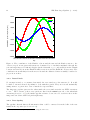
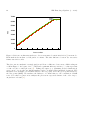
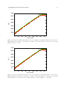
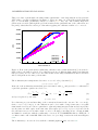
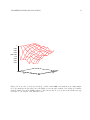
30
7.2
NIR First Stage Pipeline (v
2.348)
Ordinary Least Squares Fit
It is easy to deduce from Monte Carlo tests that the ordinary least squares fit for data measured
with some noise in the dependent variable [18, 19, 20, 14] is estimating the slope of the line
better than estimating the slope by averaging Fowler-Pair differences. The result is summarized
in Figure 12. An ideal sequence of measurements was intialized with a constant slope. Then 2N
measurements are taken: The first N are sampled at times 1, 2, . . . N , then g ≥ 0 points are skipped
and not taken into account or simply not available, and then N final points are sampled at times
N + 1 + g, N + 2 + g, . . . 2N + g. To each data point noise with the same width was added. Then the
slope was estimated by the OLS fit on one hand and by averaging the N Fowler pairs on the other
hand. This was done 2000 times, resulting in two statistics of slope errors. The root-mean-square
of the error for the OLS fit divided by the root-mean-square of the error for the MER fit is generally
smaller than one. (The case with N = 1 pair is marginal because the fits of the slope are the same
with the two estimators, so the errors are also the same for any given noise.)
The fact that both means of deriving a slope are not equivalent is obvious: One could add actually
a constant value to both values in any measurement of a Fowler pair, which would not take any
effect on the slope estimator because that constant would cancel when the difference is calculated.
The least squares estimator would be effected because the leverage arm of the two samples relative
to the center would differ.
In conclusion there is no reason to implement a separate MER data analysis because the OLS fit
outperforms it for all combinations of sample number and intermediate gap in the sample series.
Therefore only a single fitting (merging) function pipFits ols is implemented.
CARMENES-AIV04B-NIR-DCS-MAN02
31
1
0.98
0.96
0.94
ratio 0.92
0.9
0.88
0.86
0.84
0
5 10
15 20
25 30
N
35 400
5
30
20 25
15
gap
10
Figure 12: Noise ratio σOLS (α1 )/σM ER (α1 ) of OLS versus MER read analysis from a MC simulation. For small gap in the time series, the RMS error in the OLS estimator is roughly 15% smaller
than the RMS error in the MER estimator. The effect is the more pronounced the smaller the gap
is relative to the length of the full time series.