1
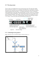
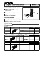
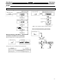
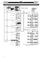
USER MANUAL
For the lab scale
MINILOOP
Table of content
1
Introduction ...................................................................................................................... 3
2
Miniloop and equipment.................................................................................................. 4
3
Operating the Miniloop ...................................................................................................... 7
3.1
Start up and shut down procedures. ........................................................................... 7
3.2
User interface ............................................................................................................. 8
3.3
Active control............................................................................................................. 9
3.4
Manual control ........................................................................................................... 9
4
The Miniloop block diagram......................................................................................... 10
4.1
The subVi’s .............................................................................................................. 10
4.2
Filters and charts. ..................................................................................................... 11
4.3
CASE structure and the controllers.......................................................................... 12
4.4
Writing the data to a file........................................................................................... 13
5
Maintenance.................................................................................................................... 14
5.1
Reservoir tank. ......................................................................................................... 14
5.2
Buffer tank................................................................................................................ 14
5.3
The slug sensor......................................................................................................... 15
5.3.1
Calibrating the slug sensor. .............................................................................. 15
5.3.2
Troubleshooting the slug sensor....................................................................... 17
5.4
Colouring matter ...................................................................................................... 17
6
References ....................................................................................................................... 18
Appendix A Equipment suppliers and prises........................................................................ 19
Appendix B Equipment manuals .......................................................................................... 20
2
1 Introduction
The Miniloop was originally constructed by Bårdsen [1] as a part of his fifth grade project
with the Department of Chemical Engineering at NTNU. Since then some work has been done
on the Miniloop by Søndrol2 as a part of his thesis. New measurements have been added and
analyzed. A new user interface has been constructed to obtain the new measurements and to
allow different control structures.
This user manual was written as a part of the thesis [2], however it is meant to be a stand
alone user manual. This means that some of the things presented in this manual can also be
found in the Diploma thesis [2].
The Miniloop is essentially very easy to use. However there are some issues the user should
be aware of. It is therefore recommended to read this user manual before performing any
experiments on the Miniloop.
3
2 Miniloop and equipment
Figure 2.1 shows an overview of the lab scale Miniloop. The different components are listed
in table 2.1.
Figure 2.1
Flow sheet for the Miniloop.
As can be seen from the figure the Miniloop has a water (WT) sorce and an air source. The
water is pumped from the reservoir into the system, while the air is let into the system from a
pressurized air outlet in the wall. The flow rate of water and air is controlled by manually
adjusting valves V1 and V2. The pipeline system is constructed of several connecting sections
of transparent plastic tubes. The pipeline is meant to imitate the pipeline topography where
gravity induced slugging occurs, which is a low point connected to an inclined section of the
pipe. At the top of the riser the multiphase flow passes the control valve before it enters the
separator. At this point the air is released out of the system through an open hole in the
separator, while the water is returned to the reservoir. To monitor the behaviour of the system
a combination of pressure measurements and slug sensors are used. The measured signals are
transmitted to a computer through the FieldPoint (FP) modules, where they can be analyzed,
stored and manipulated.
4
Table 2.1
Denote
FT.W
FT.A
P1
P2
P3
S1
S2
PU
WT
BT
ST
CV
List of equipment.
Equipment
Rate meter for water(Gemu 3021)
Rate meter for Air
Pressure sensor (MPX5100DP) Feed inlet
Pressure sensor (MPX5100DP) Valve
Pressure sensor (MPX5100DP) Separator air outlet
Slug sensor (E3X-DA-N)
Slug sensor (E3X-DA-N)
Pump (Eheim 1060)
Reservoir
Buffer tank
Separator
Control valve
Consult table A.1 for more info about the distributors and prises. More detailed information
about the different equipment can be found in appendix B. The different equipment will be
briefly discussed below.
The rate meter for water (figure 2.1) is placed in front of the mixing point of water and air.
The digital display shows the rate of water in l/min. It provides a signal between 4-20mA,
depending on the rate of flow, which is send to the computer.
The rate meter for air (figure 2.2) is placed in front of the mixing point of water and air. It
has a digital display that shows the rate of air in percent of its operating area, witch is 0-2.2
l/min. The rate meter also provides a signal between 0-5 V which is send to the computer.
The pressure sensors (figure 2.3) are one of Motorola’s differential pressure sensors that
delivers a signal between 0.2-4.5 V. The relationship between voltage and pressure is linear
and its operating area is between 0-100kPa.
The slug sensors (figure 2.4) are fibre optical sensors. Each slug sensor is made up of two
fibre optical cables connected to a sensor. The light emitted from the senor will travel out
through one of the cables and back through the other. The device will provide a signal
between 1-5 V depending on how much light is transmitted between the two cables.
The pump (figure 2.5) used is a standard aquarium pump. It can deliver up to 38 l/min and
work against a head of 3.1 m. Special care must be taken to make sure it doesn’t pump air as
this can damage the pump.
The reservoir (figure 2.6) is a cylindrical container made of transparent glass. It serves as the
water source for the Miniloop, and the water is returned to the tank from the separator.
The separator (figure 2.7) is also a cylindrical glass container with one inlet and two outlets.
The air is released to the surroundings through an open hole in the top, while the water is
returned to the reservoir.
5
The buffer tank (figure 2.8) is a cylindrical container made of transparent glass. For slugs to
appear the system needs a sufficiently large air volume. The air volume in the tank can be
altered by adding water to the tank.
The control valve (figure 2.9) is located at the top of the riser before the separator inlet. The
valve requires a 24V power supply and is controlled by a signal to the actuator between 4-20
mA. The relationship between the valve’s actuator and the valve opening is linear. To operate
the actuator an external pressurized air source of 4-8 bar is required to counteract the spring
power. The lab has its own pressurized air source, which was used for this purpose.
Figure 2.1 Flow meter
Figure 2.1 Flow meter
Figure 2.3 Pressure sensor
Figure 2.4 Slug sensor
Figure 2.5 Pump
Figure 2.6 Reservoir
Figure 2.7 Separator
Figure 2.8 Buffer tank
Figure 2.9 control valve
6
3 Operating the Miniloop
3.1 Start up and shut down procedures.
Start up
1.
2.
3.
4.
5.
6.
7.
8.
Start the computer and open the LabVIEW program miniloop.
Make sure valve V1 and V2 are closed.
Connect the power to the field point modules.
Turn the field point modules on by using the switch.
Connect the power to the pump.
Put the miniloop program into run mode.
Turn valve V2 until the desired air flow is reached.
Turn valve V1 until the desired water flow is reached.
Shut down
1.
2.
3.
4.
5.
Shut of the water supply first(valve V1 first), then the air supply (valve V2).
Disconnect the power supply to the pump
Turn of the field point modules with the switch.
Disconnect the power source to the field point modules.
Close LabView and shut down the computer.
Comments
•
•
•
The air supply must always be turned on first and shut down last. The reason is
to obtain a certain pressure inside the hose to prevent backflow of water into
the buffer tank(BT).
The pump will start to work as soon as the power supply is connected. So make
sure there is no air in the pipe leading from the water reservoir to the pump.
Also make sure that the water level in the reservoir tank is higher then the
outlet leading to the pump.
The valve will always close itself when the field point modules are turned off.
The miniloop program therefore has to be put in run mode to open the valve
before air or water is introduced to the system. Failure to do this will result in a
quick pressure build up in the pipe and a blow out of the pressure sensors.
Adjusting flow rates
During system start up it is recommended to adjust the air flow to the desired flow rate before
introducing water into the system. Once the air flow is adjusted the water flow rate can be
adjusted to the desired rate. Take note that the water flow rate will vary depending on the
upstream pressure. The water flow will normally vary around 10%. To maintain consistency
it’s recommended to use the max flow rate during these variations as the reference.
The air flow measurement is dependent on the temperature inside the measuring device. This
means that the measured flow rate of air will drop during the first minutes after start up as the
temperature inside the device stabilize it self. Because of this its not recommended to initiate
any experiments until the measurement is stable ( approx. : 5-10 mins.)
7
3.2 User interface
The Miniloop is controlled by a computer through the user interface.
Figure 3.1
User interface for the Miniloop.
The front panel has three main areas of interest. First of you have the charts used to visualize
the measurements, like pressure drop, valve opening, flow and hold up. The top chart displays
the downstream pressure, while the second one displays the upstream pressure. If anti slug
control is applied the mentioned charts will display the relevant set point. The third chart from
the top plots the flow of water into the system and an estimate of the flow through the control
valve. If a cascade controller is applied it will also show the relevant set point. The slug
sensor results are plotted at the bottom. This measurement plots the filtered signal received
from the optical sensors.
The PID control is located at the lower left corner of the screen. This is where the user
chooses witch control structure to use. The loop is set to “no control” by default, but by
clicking it you can choose from the available control configurations from a pull down menu :
The tuning parameters for the different controllers are also located here, witch means the user
can change them by simply entering the new value.
In the upper left corner of the front panel the user will find some additional indicators that
displays additional information about the system. Most measurements are already filtered to
some degree, but since the estimated flow measurement is the one most prone to disturbances,
an additional lag filter has been added. The parameters for this filter can be altered by
changing the values in the filter box.
8
3.3 Active control
To apply active control the user have to open the pull down menu in the PID control box and
choose witch control configuration to use. The control selector is set to “No control” by
default. Choosing a different control structure then this will immediately switch the system
from open loop (manual control) to closed loop (active control). The chosen controller will
use the relevant tuning parameters given in the PID control box. The default parameters will
stabilize the system at the given set point. Both parameters and set points can be altered
during active control. However one must pay close attention to the system if these values are
changed. Wrong parameters during active control can make the valve close it self, leading to a
pressure build up and a blow out of the pressure sensor. If this happens the user must switch
the control selector back to “no control” to reset the valve position and prevent the build up of
pressure.
Figure 3.2
PID control box.
3.4 Manual control
Figure 3.3
When the control selector is set to “No control” in the PID control box the
process will run in open loop mode. The user can adjust the valve opening by
adjusting the slide bar or by entering the new value for the valve opening in the
small box below.
0
Figure 3.3
Manual valve
control.
9
4 The Miniloop block diagram.
In this chapter the most important components or subVi’s in the block diagram will be briefly
explained. Understanding of the block diagram is essential if the user wish to add more code
or alter the existing code. More information about the detailed tasks of each component can
be learned by reading the text boxes inside each subVi or by using the help function in
LabVIEW.
4.1 The subVi’s
Figure 4.1
The block diagram.
Figure 4.1 shows a section of the block diagram. The yellow boxes with name tags in the
middle are different SubVi’s. Each of them contains additional code that can be accessed by
double clicking the block in the actual program. The programming follows the flow of data. A
while loop encompasses most of the code and the measurements will enter the while loop in
the wire marked with a big red X. Once it is inside the while loop it will pass from box to box
by following the different wiring.
The different subVI’s and their purpose are listed below.
Read:
Calibrate:
Value check:
Here the data is indexed and tagged.
The data is split into separate data streams and calibrated.
Here the different measurements are checked to ensure they don’t take
inconsistent values. Disturbance and noise may cause a measurement to
take illegal values i.e. a pressure becoming negative. This subVi will
remove these values and force the measurement to take values within a
given limit.
10
Density:
Flow:
Valve position:
The slug sensor signal is send to this SubVi, and the density is
calculated based on the equations inside the SubVi.
This subVi needs the density calculated in the previous subVi, the
pressure drop across the valve and the valve opening. It will then
estimate the total mass flow through the valve.
This subVi will calculate the valve opening from the actuator position.
4.2 Filters and charts.
The block diagram in figure 4.1 are marked with green, blue and red circles. They are there so
the user can quickly identify the following components.
Green circles:
Blue circles:
Red circle:
The componets inside the green circle are indicators. They plot the
corresponding data in the charts located in the front panel. The different
measurements being plotted are downstream pressure P1, upstream
pressure P2, valve position z, flow Q and W, and the slug sensor S2.
The blue circles encompass the PID Control Input Filters. These filters
apply a fifth-order low-pass FIR filter to the input value. Filter cut-off
frequency is designed to be 1/10 of the sample frequency of the input
value. Use this function to filter measured values (such as process
variable) in control applications.
The red circle encompasses a lag filter. This filter has been added to the
estimated mass flow measurement. The filter parameters can be
adjusted in the filter box on the front panel.
11
4.3 CASE structure and the controllers.
The different control structures are located inside within the case structure. New control
configurations can be included in the program by adding a new case and filling in the relevant
code. Below is an example of case 3. This is a cascade configuration that uses mass flow W in
the inner loop and upstream pressure P1 in the outer loop. The measurements and set point is
passed from the while loop to the case. The controllers then calculate the valve position and
sends it back to the while loop.
Figure 4.2
Case structure, the controller.
The PID controllers:
The actual PID controllers are located within the blue circles.
The parameters associated with the PID controller are the minmax output signals the controller can take. In case of the outer
loop, these parameters represent the values that the set point in
the inner loop may take
The tuning parameters:
These are located within the red circles. They actual values are
set in the front panel.
Set point and variable:
The set points and measurements have to be converted from
engineering units to percent of operating area, this is done in the
green circles. The parameters set here correspond to the min and
max values that the set point and variables can take.
12
4.4 Writing the data to a file.
The miniloop program will automatically write the selected data to a .txt file when the
program is stopped using the large stop button. The data will be stored in the following
format.
Table 4.1
Format of stored data.
t [msek]
S [V]
P1 [Barg]
P2 [Barg]
…
…
…
…
…
…
…
…
Qinlet
[l/min]
…
…
Westimated
[kg/min]
…
…
Z [-]
…
…
To store additional data to file use the following procedure.
1. Open the block diagram and locate the “write to file” function in the right most section of
the diagram. All the data will be collected in the yellow block, and collected in one array. Its
then send the the little white block and written to file upon termination of the program.
Figure 4.3
Create a free node.
2. By clicking the yellow box and holding you can increase the length of it, allowing more
data stream to be added to it. The box in figure 4.3 has been increased to allow 4 more data
streams.
3. The next stage is to locate the data you wish to store to the file. Then simply wire it to an
available node on the yellow box(figure 4.4). The additional data stream will now be stored to
the same file.
3
Figure 4.4
Wire the data.
13
5 Maintenance.
The Miniloop do not require much maintenance. However the user should be aware of a few
things.
5.1 Reservoir tank.
The user has to make sure the liquid level in the reservoir tank doesn’t get to low. From figure
5.1. one can see that there are two tubes connected to the tank. The top tube is connected to
the separator, and the water will return to the reservoir through this tube. The second tube is
connected on the flat end side of the tank. This is connected to the pump witch pumps the
water into the Miniloop. Before the pump is turned on the user has to make sure the liquid
level is higher then this outlet, if not air may enter the tube. This can damage the pump, and in
the worst case damage it. The water level should at least be 3 cm higher then the outlet.
Additional water can be added to the tank through the open hole on the flat side, above the
outlet. There is a water source available with a long enough hose in close proximity to the
loop. To empty the tank the user can remove both tubes and pour the liquid into the sink.
If the user wish to clean the tank with water make sure it is not to hot. Using only hot water to
clean the tank may cause the glass to crack.
Figure 5.1
Reservoir tank.
5.2 Buffer tank.
The buffer tank is used to create enough upstream volume for the gas. This is a prerequisite
for slugging to occur. The volume available for the gas will influence the amplitude of the
pressure oscillations. The volume can be altered by adjusting the liquid volume inside the
tank. To add more water the user has to disconnect both tubes leading to it. As for the
reservoir tank the buffer tank mustn’t be cleaned with to hot water as this may result in
cracks.
Figure 5.2
Buffer tank.
14
5.3 The slug sensor
There are quite a few things that can cause the slug sensor to fail. The slug sensor should
always be checked to make sure it is operating as intended before an experiment is started.
The easiest way to check the sensor is to make sure the slug sensor chart in the user interface
(miniloop program front panel, figure 3.1) is taking values between 1 and 5. It should be 1
when measuring pure water and 5 when measuring only air. If this is not the case, something
is causing the sensor to malfunction. Take note that the problem may not be with the sensor
itself, but with the Miniloop. This chapter will show the user how to reconfigure the sensor
from start. However, if the sensor is malfunctioning consult the trouble shooting in chapter
5.3.2. Figure 5.3 shows the actual sensor and the different settings on it.
Figure 5.3
The sensor settings.
5.3.1 Calibrating the slug sensor.
Step 1 ) Reset the sensor to default settings as shown in figure 5.4.
Figure 5.4
Resetting the slug sensor to default setting.
15
Step 2) Recording the sensor value corresponding to pure water..
Record the value showing in the sensors digital display when measuring pure water. The
display will vary between 0 and 4000. The value will depend on the amount of light being
returned to the sensor. 4000 means all the light has returned(as for air). When measuring
water the display should take a value between 500 and 1500. If the value is higher then 1500
the water is absorbing to little light. Add more colouring matter as described in chapter 5.4
until the value is within the given bounds.
Step 3)Setting the lower limit for monitoring.
The user must then set the lower limit for monitoring a bit higher then the value recorded for
pure water. This is done to remove the unwanted spikes caused by the surface of the phase
transitions. If the digital display is showing a value of 1000 for pure water the user should set
the lower limit for monitoring at 1200.
Press and hold the mode button
until the display shows :
Then press and hold the teach button until the display show the desired value for the lower
limit as shown in figure 5.5. The lower limit will increase in increments of 100. When the
desired value is reached release the teach button and switch the mode selector back to run
mode.
Figure 5.5
Setting the lower limit for monitoring.
16
5.3.2 Troubleshooting the slug sensor.
This chapter should solve the most common problems with the slug sensor.
Problem:
The slug sensor chart in the user interface is not taking values between 1 and 5.
The slug sensor chart is showing values below 5 for pure air when it should show 5.
Solution:
When there is only air in the tube no light should be absorbed, and the
sensor should show its max value. Check the digital display on the
sensor. The display should show 4000 when only air is present. If it
shows less something is interfering with the light beam. Make sure the
sensor is not placed on a stained part of the pipe as stains may block
some of the light, moving it to a different location or changing the
stained section of pipe will most likely solve the problem. The cables
may also be bent resulting in a failure within the cable. Make sure the
cable is running loosely and smoothly from the sensor to the bracket
without to large angels.
The slug sensor chart is showing values higher then 1 for pure water when it should
show 1.
Solution:
Most likely the lower limit for monitoring is set to high, or there is too
little colouring matter in the water. Check step 2 in chapter 5.3.1.
5.4 Colouring matter
The colouring matter used to give the water a blue colour is called Vulcanosol-Blau 684.
More colouring matter can be obtained from Engineer Arne Fossum at his office in K3-019.
Very little substance is needed to dye the water. It’s recommended to gradually add small
amounts of substance until the desired slug sensor value has been achieved. The system
should be set to pump water through the system to disperse to substance properly.
One spatula is enough to dye all the water in the system if the reservoir tank is half full.
17
6 References
[1] Bårdsen, I., “Anti-slug control for two phase flow. Experimental verification (In
Norwegian),” NTNU, autumn 2003.
[2] Søndrol, M., “Anti-slug control. Experimental testing and verification,” NTNU, spring
2005
18
Appendix A
Equipment suppliers and prises
Table A.1 lists the suppliers and prises for the different components in the Miniloop.
Table A.1
List of equipment, suppliers and prises.
Equipment
Type
Delivered by
Prise
[NOK]
3991
4502
Rate meter for water
Control Valve
Gemu 3021
Gemu 554
Rate meter for air
D-5110-HAB
J.S. Cock 3991
P.O.BOX 68 Stovner
N-0913 OSLO
Phone:+47 22 21 51 00
Flow-Teknikk as
Olav Brunborgsv.27
P.O.BOX 244
1377 Billingstad
Phone : +47 66 77 54 00
A1-Module
AO-Module
Termination base
Communication
module
Signal transducer for
the control valve
FP-AI-100
FP-AO-210
FP-TB-2
FP-1000
National Instruments 2745
P.O.BOX 177
N-1386 Asker
Phone:+47 66 90 76 60
2745
3555
1512
3105
MICROANALOG
DC/DC Select
1550
3 x Pressure sensors
MPX5100DP
JF.Knudtzen AS
P.O.BOX 160
N-1378 Nesbru
Phone:+47 66 98 33 50
Silica/Avnet Nortec AS
P.O.BOX 63
N-1371 Asker
Phone:+47 66 77 36 00
Pumpe
3x Optic sensors
Eheim 1060
E3X-DA-N
Petshop at city syd
Omron
P.O.BOX 109 Bryn
N-0611 OSLO
Phone:+47 22 65 75 00
1566
2825
3x Tanks
Tubes
Transparent glass
Silicone
Produced by NTNU
9000
4000
9914
796
19
Appendix B
Equipment manuals
The equipment manuals are large and comprehensive. Because of this not all of them will be
appended to this user manual. However the table below will list where they can be found.
The manuals for the equipment listed in table B.1 can be found in appendix B in [1], while the
manuals listed in table B.2 can be found in this appendix.
Table B.1
Reference to equipment manuals.
Equipment
Pressure sensor
Signal transducer (control valve)
FieldPoint A1-Module
FieldPoint AO-Module
FieldPoint Terminal base
Table B.2
Page
43
51
55
69
81
Reference to equipment manuals.
Equipment
Rate meter for liquid
Rate meter for gas
Optic sensor
(In Danish)
Appendix
B1
B2
B3
20
Flow-Teknikk as
Mass Flow Meters and
Controllers for Gases
MASS-STREAM®
M+W Instruments
Your partner
Key Facts
M+W Instruments was founded in 1988 and has always specialised
in mass flow meters and controlers.
In 1995, M+W Instruments was the first company to introduce the
direct measuring principle for thermal mass flow meters with the
sensor following the constant temperature anemometer principle.
In 1997 M+W Instruments joined the Bronkhorst Group.
Today we are working along side more than 20 distributors worldwide. You will find your personal contact on the back page of this brochure or under www.mw-instruments.com.
Our intruments are suitable for the use in the pharmaceutical, chemical and semiconductor industries as well as in the gas and food
industry. Of course we are your competent address for special solutions.
Content
Key Facts, Working Principle
“MASS-STREAM®”
Mass Flow Meters
Mass Flow Controllers
Conversion factors,
Flow profile sensitivity
Seite
Seite
Seite
Seite
2
3
4
5
Seite 6
Pressure drop
Model number identification
Technical specifications
Ultra fast sensor, Digital version
Readout systems
Contact addresses
Seite
Seite
Seite
Seite
Seite
Seite
Principle of Operation
Basically the instruments consits of a metal block with a straight
bore. Two stainless steel probes protrude inside the bore; a heater
probe and a temperature probe. A constant difference in temperature (∆T) is created between the two and the energy required to maintain this ∆T is dependent of the mass flow rate.
Seals
Body
Heater
Sensor
Generally speaking we can say that the higher the flow the more
energy is required to maintain the chosen ∆T, which is usually
approx. 38° C. Overall we can state that King’s law applies to the
relationship between heater energy and mass flow, and the following formula can be derived.
n
P=P0+CØm
P
P0
C
Øm
n
2
Basic structure of the MASS-STREAM®-flow sensor
= total heater power
= heater power offset at zero flow
= constant
= mass flow
= dimensionless number (typ. 0.5)
Loop to control the heater current (CTA)
> flow sensor <
in Wheatstone
bridge
configuration
Flow
Constant
∆T control
Signal conditioning
Nulling
and
amplification
Linearisation
and
amplification
Output Voltage
or Current
7
8
9
10
11
12
“MASS-STREAM®”
Features and Applications
Worth knowing
MASS-STREAM® is the synonym for a metering principle having the
following advantages:
Smallest standard range
0,005...0,1 ln/min (Air)
Highest standard range
100.0...7500.0 ln/min (Air)
Lower and higher ranges available on request.
Features
◆
◆
◆
◆
Low pressure drop
Rugged design
Lower sensivity concerning dirt and humidity
Measuring independent of pressure and temperature changes
◆ Installable in virtually any position
◆ No moving parts
◆ Bodies in stainless steel or as a more economical
aluminium version
Applications
◆
◆
◆
◆
◆
◆
◆
◆
Gas consumption metering
Exhaust gas metering
Semiconductor industry
Analytical intruments
N2/O2-generators
Fuel cells
Mechanical engineering
And much more
Options
◆
◆
◆
◆
◆
“Low ∆P” version
Integrated totalisation
Integrated actual display
Integrated setpoint potmeter
Readout systems
3
Model D-6210 MFM
Mass Flow Meters
Principle of Operation
Flowmeters of M+W Instruments are suitable for all kinds of applications in industrial, chemical, medical and laboratory
environments.
Main advantages of these instruments
are:
◆ Usuable for virtually every kind of
gases
◆ No moving parts
◆ Very low pressure drop
◆ Unique all stainless steel sensor
◆ Pressure and temperature independent metering system
◆
◆
◆
◆
◆
◆
The 62xx series working principle is shown
on page 2.
For lower flow values the by-pass measurement principle is applied.
Installable in virtually every position
No inlet pipes needed (62xx series)
Optional with integrated flow display
Optional with totalisation
No maintance needed
Two body materials on stock
(others on request)
Model
D-5110
D-6210
D-6230
D-6250
Standard Flow Capacities
Mass Flow Meters
Model
Flow capacitiy (Air)
(intermediate ranges available)
D-5110 - AAA - BB - AA -
12 - A - A - A
22
52
13
23
53
14
0.005...0.1
0.010...0.2
0.025...0.5
0.05...1.0
0.1...2.0
0.25...5.0
0.5...10.0
ln/min Air
ln/min Air
ln/min Air
ln/min Air
ln/min Air
ln/min Air
ln/min Air
D-6210 - HAB - BB - AA -
53 - A - A - A
14
24
0.25...5.0
0.5...10.0
1.0...20.0
ln/min Air
ln/min Air
ln/min Air
D-6230 - HAB - BB - AA -
24 - A - A - A
54
15
1.0...20.0
2.5...50.0
5.0...100.0
ln/min Air
ln/min Air
ln/min Air
D-6250 - HAB - CC - AA -
15 - A - A - A
25
45
5.0...100.0
10.0...200.0
20.0...400.0
ln/min Air
ln/min Air
ln/min Air
D-6270 - HAB - CC - AA -
55 - A - A - A
16
26
25.0...500.0
50.0...1000.0
100.0...2000.0
ln/min Air
ln/min Air
ln/min Air
D-6280 - HAB - DD - AA -
36 - A - A - A
46
56
150.0...3000.0
200.0...4000.0
250.0...5000.0
ln/min Air
ln/min Air
ln/min Air
66 - A - A - A
76
300.0...6000.0
375.0...7500.0
ln/min Air
ln/min Air
D-6290 - HAB - DD - AA -
Higher flows and other current junctions on application.
4
A
95
95
95
95
B
G1/4”
G1/4”
G1/4”
G1/2”
C
G1/4”
G1/4”
G1/4”
G1/2”
D
30
30
30
30
F
90
90
90
90
G
92
92
92
92
H
35
35
35
35
Model D-6270
Model
A
B
C
D-6270 116 G1” G1”
D-6280 116 G1” G1”
D-6290 143 G1” G1”
All specifications subject
to change without notice.
D
F
G
H
50 123 125 35
70 141 143 35
110 171 173 35
Model D-5121 MFC with LCD display
Mass Flow Controllers (MFC)
Principle of Operation
Based on the concepts of our flow meters;
compact flow controllers are also available.
When higher flows are needed an external
valve is employed.
The modular construction solenoid valve
is integrated to the base when flows are
up to approx. 500l/min. N2 equivalent.
The following kvs-values are available:
6,6E-2, 0,35; 1,0;
(for higher values please contact factory)
Features
◆ Suitable for almost all gases
and mixtures
◆ No moving parts in the sensor
◆ Good response times
◆ PI-control loop
◆ No inlet pipe necessary
(D-62xx series)
◆ Optional: integrated actual flow
display
◆ Optional: integrated totalisation
display
◆ No maintainance required
◆ Almost independent to attitude
Model
D-5111
D-5121
D-6211
D-6231
A
95
95
95
95
B
G1/4”
G1/2”
G1/4”
G1/4”
C
G1/4”
G1/4”
G1/4”
G1/4”
D
30
30
30
30
F
90
94
90
90
G
92
96
92
92
H
35
35
35
35
Standard Flow Capacities
Mass Flow Controllers
Model
Flow capacitiy (Air)
(intermediate ranges available)
D-5111
- AAA - BB - AA - 12 - A - A - A
22
52
13
23
53
14
0.005...0.1
0.010...0.2
0.025...0.5
0.05...1.0
0.1...2.0
0.25...5.0
0.5...10.0
ln/min Air
ln/min Air
ln/min Air
ln/min Air
ln/min Air
ln/min Air
ln/min Air
D-5121
- AAA - BC - AA - 14 - A - A - A
24
54
0.5...10.0
1.0...20.0
2.5...50.0
ln/min Air
ln/min Air
ln/min Air
D-6211
- AAA - BB - AA - 53 - A - A - A
14
24
0.25...5.0
0.5...10.0
1.0...20.0
ln/min Air
ln/min Air
ln/min Air
D-6231
- AAA - BB - AA - 24 - A - A - A
54
15
1.0...20.0
2.5...50.0
5.0...100.0
ln/min Air
ln/min Air
ln/min Air
D-6251
- AAA - CC - AA - 15 - A - A - A
25
55
5.0...100.0
10.0...200.0
20.0...400.0
ln/min Air
ln/min Air
ln/min Air
D-6271/004 - AAA - CC - AA - 55 - A - A - A
16
20.0...500.0
50.0...1000.0
ln/min Air
ln/min Air
Higher flows and other current junctions on application.
Model D-6251
Model A
B
C
D F G H I
D-6251 145 G1/2” G1/2” 50 132 45 95 45
D-6271 Dimensions please on application
All specifications subject
o change without notice.
5
Conversion factors
The MASS-STREAM®-Series flow meters are normally calibrated on air.
For use on other gases than air a conversion factor must be applied.
This factor is determined by applying a complex formula.
However, for a number of common gases you will find the values
below:
Conversion factor table
(Ln: 1013mbar und 0°C air temperature)
Series / Gas
Air
Ar
CH4
C2H2
C2H4
C2H6
C3H8
C4H10
C5H12
CO
CO2
D-62xx
1.00
2.01
0.67
0.75
0.89
0.89
0.63
0.42
0.25
1.04
1.20
D-51xx
1.00
1.40
0.76
0.61
0.60
0.60
0.34
0.25
0.21
1.00
0.74
Best accuracy is reached by calibrating the instruments und actual
process conditions. The conversation factor introduces an additional
error in abolute accuracy in order of:
CF ≥ 1 : 2xCF in % FS
CF ≤ 1 : 2/CF in % FS
Series / Gas
D-62xx
H2
He
HCL
N2
NH3
NO
N2O
N2O2
O2
Xe
Factors for further gases available on request.
0.15
0.24
1.58
1.00
0.80
1.02
1.15
1.00
0.98
6.08
D-51xx
1.01
1.41
0.99
1.00
0.77
0.97
0.71
1.00
0.98
1.38
When using our D-62xx serie with balloon gases like helium and
hydrogene it is always recommended to make use of the optional gas
calibration.
Flow profile sensivity
Normally mass flow measurement principles are sensitive to variations in the shape of the flow profile.
6
The MASS-STREAM®-Flow meters has been designed in such a way
that there is always a fully developed flow profile in the metering
section ans is thus virtually insensitive to changes upstream
piping conditions.
Pressure drop
The pressure drop of the instruments (serie D-62xx) is almost comparable to a straight run of pipe of the diameter ans is thus negible.
the flow profile. These meshes create a certain pressure drop as can
be seen from the table set out below.
However, to make the instruments insensitive to upstream piping
configurations, a number of mesh screens are required to condition
For further informations please contact factory.
legend
∆P (mbar)
D 6210
D 6230
D 6250
D 6270
D 6280
D 6290
flow air (ln/min)
In some applications a very low pressure drop is required. To fulfil
these inquires we are able to build a special version of our instruments where the pressure drop is extremely low.
For further information please refer to the second table set
out below.
legend
∆P (mbar)
D 6210
D 6230
D 6250
D 6270
D 6280
D 6290
flow air (ln/min)
7
Model Number Identification
Options and Model Numbers MASS-STREAM®
D
NNNN
Base model
D-511 = low flow
D-512 = medium flow
D-519 = specify
D-621
D-623
D-625
D-627
D-628
D-629
=
=
=
=
=
=
4 mm
8 mm
16 mm
32 mm
56 mm
84 mm
AAA
AA
AA
Gas connection (in/out) /
Option 2
Internal thread
BB = G1/4
CC = G1/2
DD = G1
EE = G5/4
ZZ = specify
NN
0 = Mass flow meter
1 = Mass flow controller
12 = 0.1 ln/min
22 = 0.2 ln/min
52 = 0.5 ln/min
Fittings
11 = 1/8” OD
22 = 1/4” OD
33 = 6 mm OD
44 = 12 mm OD
55 = 1/2” OD
66 = 20 mm OD
99 = specify
13 = 1 ln/min
23 = 2 ln/min
53 = 5 ln/min
14 = 10 ln/min
24 = 20 ln/min
54 = 50 ln/min
B = 24 Vdc
C = 15 Vdc
Z = specify
Output
A = 0-5 Vdc
G = 4-20 mA
(sourcing)
Style / Option 1
F = controller N/C
H = sensor only
Z = specify
A
Flow rate (Air) / Option 4
Supply Voltage
Function
A
A
Seals /
Option 3
V
E
P
Z
=
=
=
=
Viton
EPDM
PTFE Elast.
specify
15
25
45
55
=
=
=
=
100
200
400
500
ln/min
ln/min
ln/min
ln/min
16 = 1000 ln/min
26 = 2000 ln/min
36 = 3000 ln/min
46
56
66
76
99
=
=
=
=
=
4000 ln/min
5000 ln/min
6000 ln/min
7500 ln/min
specify
Display /
Option 5
0
A
B
Z
=
=
=
=
none
flow (in %)
summary
specify
Material
A = Aluminium
S = SS 316
Z = specify
Sensortyp /
Option 6
S = standard
FR = fast response
Bus Connection /
Option 7
A = analog
DP = digital / Profibus
DN = digital / device net
DR = digital / RS 232
DF = digital / Flow Bus
Enquiry and Ordering Information
In order to supply the correct instrument for your application we
request you to state: type of gas, flow range, operating temperature
and pressure (for controllers supply pressure and back pressure),
electrical connection, desired output signal, type of process connection and seals.
Based on this information we perform the following actions/
calculations:
8
◆ Convert the desired flow to Air-equivalent flow, i.e., divide the
desired flow by the conversion factor.
◆ Only for controllers, check if the pressure differential across the
valve (∆P) is within the limits.
◆ Only for controllers, check if the calculated Kv-value is within
the specifications allowed.
Technical Specifications
Measurement System
Accuracy (based on air calibration)
Repeatability
Time constant (63.2%)
Pressure sensitivity
Attitude sensitivity
Leak integrity
RFI
± 3% FS incl. non-linearity (better one’s on request)
± 0.5% FS (better one’s on request)
τ = 0.7 sec (standard, better one’s s. p. 10)
0.2% / bar typical (air)
± 0.1% °C
-9
< 2 x 10 mbar l/s He
According to CE
Operating Limits
Range
Type of gases
Temperature
Pressure
Warming up time
Installation
Series D-5100…
Series D-6200...
3…100%
All gases compatible with materials chosen
0…70°C
10 bar; higher on application
30 min for optimum accuracy;
within 30 sec for accuracy ±4% FS
10 D straight pipe upstream
Unrestricted
Mechanical Part
Sensor
Body
Sieves / rings
Protection
AISI 316L
AISI 316L or Aluminium (anodised), please specify
Stainless steel / teflon
IP40 (IP 65 on application)
Electrical Properties
Supply voltage
Current peak values
Series D-5100...
Series D-6200...
Control valve, if applicable
Output signal
Cable
24 Vdc ±10% or 15 Vdc ±10%
75 mA max.
Inrush current
250 mA max.
No flow
75 mA max.
100% flow
175 mA max.
Add 250 mA max.
0…5 Vdc or 4…20 mA
6-wire DIN or 15-wire SUB-D
9
Ultra-Fast Sensor
"Fast response” version
M+W Instruments Mass Flow Meters and Controllers are used for a
wide variety of applications and for this reason the sensor has been
set up with "smooth-response” characteristics thereby avoiding any
possible overshoot of the setpoint.
There are, however, applications where the response time of the sensor or the control valve is the decisive factor and for these applications M+W Instruments has developed a sensor with the following
features:
Seals
Body
Heating System
Heater
Flow
Response time (5τ): up to <100ms
When using this sensor in connection with a flow controller the following response times are possible:
Response time (5τ): up to <1,5s
Digital version
All our standard products are equipped with an analog pc-board, a
feature that ensures that they are very economically priced.
However, our well thought-out modular system allows us to offer a
digital pc-board as well thereby giving the options of analog voltage or current output together with Profibus DP, Device Net, RS 232
or Flowbus protocols.
Flow Controller response times down to 0.5 sec and less are possible when using the "fast response” sensor.
10
If even faster times are required then we would recommend using
this sensor in conjunction with our digital pc-board. Further information is available within the section headed "Digital version”.
Dimensions as standard, s. p. 4/5
Model number identification, s. p. 8
Readout Systems
Model D-15
with integrated Power Supply
General
This series comprises standard types for
use with analog mass flow meters and
controllers. The most commonly used
functions are offered in compact single
channel table top housing, DIN panel
mount cassette and multi-channel versions in 1/2 19” or 19” table top or rack
housing.
Functions
◆ Power Supply for MFM/MFC
◆ Indication of flow rate
◆ Totalization
◆ Setpoint-potentiometer
Electrical data
◆ Power supply 110 or 230 Vac,
50/60 Hz.
◆ Suitable for connection of instruments with output signal 0…5 Vac
◆ Sub-D socket for instrument
connection
◆ Max. power +24 Vac,
0.5 A per channel
Model number identification
Code
D - 11
D - 12
D - 13
D - 14
D - 15
D - 16
D - 19
Code
- 00
- 10
- 20
Code
- 00
- 01
- 02
- 03
Code
- 10
- 11
- 12
- 13
Code
- 20
- 21
- 22
- 23
Code
- 30
- 31
- 32
- 33
Code
- 40
- 41
- 42
- 43
Housing
1/2 19” table top
42 TE
19” table top
84 TE
1/2 19” rack
42 TE
19” rack
84 TE
Table top cassette
14 TE
Panel mount cassette
14 TE
Other/specify
Supply voltage
100...240 Vac
230 Vac
110 Vac
Modules with blind front (14TE)
Rearpanel with power supply + mains entry (incl. cable)
Rearpanel with power supply / sub D connector
Rearpanel with Sub D connector
Rearpanel blind
Modules with flow indication (actual display) (14TE)
Rearpanel with power supply + mains entry (incl. cable)
Rearpanel with power supply / sub D connector
Rearpanel with Sub D connector
Rearpanel blind
Modules with indication of totalised flow (14TE)
Rearpanel with power supply + mains entry (incl. cable)
Rearpanel with power supply / sub D connector
Rearpanel with Sub D connector
Rearpanel blind
Modules with flow indication + control (14TE)
Rearpanel with power supply + mains entry (incl. cable)
Rearpanel with power supply / sub D connector
Rearpanel with Sub D connector
Rearpanel blind
Modules with total flow + control (14TE)
Rearpanel with power supply + mains entry (incl. cable)
Rearpanel with power supply / sub D connector
Rearpanel with Sub D connector
Rearpanel blind
Model D-11
Model D-14
11
Distributor:
Flow-Teknikk
as
Olav Brunborgsv. 27, Postboks 244, 1377 BILLINGSTAD
Tlf.: 66 77 54 00 Fax: 66 77 54 01 E-post: [email protected] www.flow.no
'LJLWDO ILEHUIRUVW UNHU
(;'$1
! " #$%% !& ' ( ) * ++ ,
'- *
. */
+
7\SHRYHUVLJW
! "
#
$
'
$
$
'
$
%
&
(
)
*
*
! "
+
' +
$
$
$
$
! "
,-
+ +
$.
/-
+
01- !
1 -+ +
# ##
#
-
0'+ 1 #. +
+ 0
23-
4
44
%
&
(
)
+
' +
$ 5
6
$ 5
6
$ 5
6
$ 5
6
! " 0 7
+
78 ' +
7
9+ 8 0' +
+ ' 0:
- 1
7
; -0+0- ; -
; %
$&
M4
E3X-DA2-N
E3X-DAB11-N
! "
#
$
1.4-mm dia.
(0.02-mm
dia.)
'%
1.4-mm dia.
(0.01-mm
dia.)
''%
0.9-mm dia.
(0.01-mm
dia.))
''%
7LOODGHOLJ
E¡MQLQJV
UDGLXV
25 mm
(
E3X-DA2-N
3-mm dia.
%
$
M3
' (
E3X-DA2-N
2-mm dia.
E3X-DA2-N
'''%
25 mm
%
$&) ) #
$&
2
$
'*%
'+',,
M14
M4
! "'
#
2
7LOODGHOLJ
E¡MQLQJV
UDGLXV
$) #- . M3
2
$
M3
2
/
' (0 1 2(') 32!
2 '+',,
2
2-mm dia.
90 mm (40 mm) 1.2-mm dia. 2
'+',,
'''
(7&%
(7&%
(7&)
(7&)
'6
''6
'
''
M4
( ): E32-TC200B4
2,() 32!
2 90 mm (40 mm) 0.9-mm dia.
2
( ): E32-TC200F4
4
2! (
32!
#5
M4
M3
2
2
(
$
-12
7 1
2
(
$
-12
7 1
2
%
0
M4
2
M3
1.5-mm dia.
3-mm dia.
2
2
'''3
2
'&%
''&
1 1-mm dia.
2
#
7 1
-! : + + 5' +8 ++67
7 + 8 ! + ++
+ '++ ++
+
38
'+ '+ <<< -! +-
37
= 9+ '+ 7
= + -! 2(" < 7
$1
-1
!2
"0
8#
,-+ *,-+
8#
,-+ *,-+
''
2
'&
'96
'.
'.&
':&
'''
2
7LOODGHOLJ
E¡MQLQJV
UDGLXV
2
2
7 (
(
0
1 .,q+"0 1 0
8#
&,-+ .,-+
0
-2!
$
"0
-2!
! "&
#
$1 .,q+"0
8#
&,-+ .,-+
%
/
2
$1 ',,q+0
0 "
8#
&,-+ ',,-+
:
2
2
3.5 x 3-mm dia.
& 2- -2!
2
2
1 1
,
''&
'$'
'9;
'9
'9<
2
1 1
, 0 1 1 1 0 7<.,
2
#
2
7 1
-! : + + 5' +8 ++67
7 + 8 ! + ++
+ '++ ++
+
38
'+ '+ <<< -! +-
37
= 2
+ '
= 7 '' - <q$7
= 9+ ' -! -+7
= 9+ '+ + 7
= + 7
9+ 8 0' +
+ ' 0:
- 1
7
; -0+0- ; -
; %
$9
"
2
2
$&
2
(
2
#
$9
'='
'='%
'=''%
2
7LOODGHOLJ
E¡MQLQJV
UDGLXV
'=%
$
(
!
(
"' :#
1
'=+',,
$
2
/
'(. (0
32! 2 2
2.5-mm dia.
'=+',,
('&%
('&%
(' (0
32! 2 ,(> (0
? ,(. (0
? 4
2! (
32!
#
5
2
1.2-mm dia.
2
0.5-mm dia.
2
2-mm dia.
('&)
('&)
'=
'=
2
2
'=6
'='6
(
$
-12
7 1
2
j
j
j
1.5-mm dia.
'='
#
'=
j
'='3
'=''3
7 *+ -+' :7
7 ' 1'+ 1 - >0 -! 7
= 2 ' 0'+ --+
= 9+ '+ + 7
$SSOLNDWLRQ
+@
$9 ?@0
2!- $ "
j
$ ?@0 2!-0 #
.A3A+
$ ?@0 2!-0 #
.A3A+
' ( ?@0
2!-0 #
,( ,(9
' ( ?@0
2!-0 #
,(. 9 (0
j
j
j
j
j
j
j
'++',,
7LOODGHOLJ
E¡MQLQJV
UDGLXV
'='%
'+
'+&
'+&'
'='
' (0
1 /1
( ?@0
2!-
!
(
". :#
1
'=&%
'='&
$SSOLNDWLRQ
$1
-1
!2
"0 8
#
,-+ *,-+
$1 .,q+"0
8
# &,-+
.,-+
2
!
(
". :#
1
7LOODGHOLJ
E¡MQLQJV
UDGLXV
'='
'=.
2
,,q+"0
$1
# / 8
#
&,-+ ,,-+
#
$ "
2
'=9
7 *+ -+' :7
7 ' 1'+ 1 - >0 -! 7
= 9+ - !
-! + -+7
= 2 ++8 '+ -! 0'+ --+7
= ?7 '' - <q$7
=
= 9+ '+ 7
2
+ ' - $-37
$SSOLNDWLRQ
1 # 2
2
0 7<99
!" !" !"#
!" 2
!"#
!
(
"' :#
1
$
7LOODGHOLJ
E¡MQLQJV
UDGLXV
'=9<
'6'
B6
-2
'69
B6
-2
'%.9
'%.9'
'%'&%
!" <
2
1
-2!0
8
# &,-+ ,.-+0
7<.,
2
1
-2!0
7<.,
2
!" 2
H
H
H
'%'.%
H
H
H
'%'.
2
'%'.
4
#
$
1 2
2
'%'.
7 *+ + : -! ' + -
3 7
7 ' 1'+ 1 - >08 -! 7
= 9+ '+ 7
= 2 ++8 '+ -! 0'+ --+7
6SHFLILNDWLRQHU
$ % &''
C<C #
D=C
D=9
D='C
D=*
D=3C
D=&
<C< #
D=&C
D=>
D=.C
D=
-
/
/
%/ 2
2/
#! $ r %& '**! ** % +
2#
,'
!#/
6 7 +
#'
8,':';</ + = $ 8,'> <
?, @,/
7 +
#'
8,':';</ + = $ 8,'> <
D=&&
!" *!> !"# 8'/
7 +
#'
8,':';</ + = $ 8,'> <
4
#
8CA8 #
CFCC 8G << 8 ,! ": ?,!!?#,'H :!# <#'
/
+H #* </ +H <G# IF' I =!<
C ":
?,!!?#,'H
:!# <#'
/
+H
'#* </
+H <G#
IF' I =!<
CFCC 8G <<
8 ,! ":
?,!!?#,'H
:!# <#'
/
+H
#* </ +H <G# IF'
I =!<
#
!# < #! $& :
3/ 2
I
= # *,!'##& ,'#!;# < 8 ;< <& < < *"=' <
6
J;*'G<G* ,/ 8,' '8# !!' '#
J# ' ,/ 8,' '8# !!' '#
J;*'!, <# ? ,/ 8,' '8# !!' '#
2-
K?G !!' ;! #,
#
#
L,' # 8'8!#
'/ #! H #! M;#' *' < 8 & ,< #! *' < 8 #
2 J'' '## !>
< G! !=#
E
*!>='' '## #! & G= # <#= ='' ,<" =
@;!<G 8,' # #!! #!:< #! 8:' #!! <
#
O=' ,< ' <' ' !' G' 8 J'' '##
!>
< G!
!=#
=/
P< < #,' ,' <& <
# *!> ' ,< <' !< !!
= <'/ :# = <& *',? #
= < !!' !,< :'<'8 = <
/ !< !!
,'
!FC GMFC != = <
=/ !< !!
,'
! ,< ,
= # = <
F#
@;!<G 8,' # #!! ,*# ' = GM!* 8 G>*'8!G < 8; #,
8
/
Q!!
*/ & O+ +H J,!!>/ & O+ +
8#
'8#/
8
##-
'8# ,< ,*:=' </ % #, S% ; #! < !!' , 7
@: = $
2
R <';** #! 8,'#''/ -$ #! -$
R <';** #! 8,'#''/ -$ #! -$
R <';** #! 8,'#''/ -$ #! -$
; #! < !!' , I*:=' </ -$ #! -$ ; #! < !!' , & $ = F TU ;#
#! TU& ,::!# *!#; !!' F?Q #
' '# < & V ,< W
F ?Q < < G=' '# < & V ,< W
/
3/
RC
Y:! J#
Y:! J#
Y:! @S #
$ <
$ <
$ <
$ <
$ <
$ <
$
G#
CK
=
C,!>?':, #
-2
RC
<!FZ* #';#, =M! <
*UDILVNH 'DWD
2
!" ' ?7 1
07
()*#+,+
()*#+,+
%*
%*
$%!& ' $%!& ' $%!& ' $%!& . (!&#
()*#+,+
%*
()*#"&,
%!&-
(!&#
()*#+,+
%*
$%!& . $%!& . (!&#
()*#&, %!&
()*#&, %!&
# !" : ' ?7 1
07
(!&#
()*#+,+ %*
()*#+,+ %*
!
$%!& ' ()*#&,
%!&
$%!& ' $%!& ' (!&#
$%!& . $%!& . $%!& . ()*#&, %!&
%% !" * ?7 1
07
"#$ ()*#&, %!&
$%!& ' $%!& ' (!&#
()*#+,+ %*
$%!& . ()*#+,+
%*
$%!& . ()*#+,+
%*
(!&#
()*#&,
%!&
$%!& ' $%!& ' $%!& ' # !" : ' ?7 1
07
()*#&,
%!&
$%!& . ()*#+,+
%*
(!&#
()*#&, %!&
$%!& . $%!& . ()*#+,+
%*
(!&#
()*#+,+ %*
(!&#
()*#&, %!&
'ULIW
8GJDQJVNUHGVO¡E
C
$
=1
RQTK I
FI
Y I
FI
RQTK I
FI
Y I
FI
CC
S
RQTK I
FI
Y I
FI
6
RQTK I
FI
Y I
FI
Hændelse ON
Hændelse OFF
/
Udgangsindikator ON
(orange)
OFF
UdgangsON
transistor
OFF
Belastning ON
(relæ)
OFF
(mellem brun og sort)
Hændelse ON
Hændelse OFF
/
Udgangsindikator ON
(orange)
OFF
UdgangsON
transistor
OFF
Belastning
ON
(relæ)
OFF
(mellem brun og sort)
Hændelse ON
Hændelse OFF
/
Udgangsindikator ON
(orange)
OFF
UdgangsON
transistor
OFF
Belastning ON
(relæ)
OFF
(mellem brun og sort)
Hændelse ON
Hændelse OFF
/
Udgangsindikator ON
(orange)
OFF
ON
Udgangstransistor
OFF
Belastning
ON
(relæ)
OFF
(mellem brun og sort)
Hændelse ON
Hændelse OFF
/
Udgangsindikator ON
(orange)
OFF
UdgangsON
transistor
OFF
Belastning ON
(relæ)
OFF
(mellem brun og sort)
Hændelse ON
Hændelse OFF
/
Udgangsindikator ON
(orange)
OFF
UdgangsON
transistor
OFF
Belastning
ON
(relæ)
OFF
(mellem brun og sort)
Hændelse ON
Hændelse OFF
/
Udgangsindikator ON
(orange)
OFF
UdgangsON
transistor
OFF
Belastning ON
(relæ)
OFF
(mellem brun og sort)
Hændelse ON
Hændelse OFF
/
Udgangsindikator ON
(orange)
OFF
UdgangsON
transistor
OFF
Belastning
ON
(relæ)
OFF
(mellem brun og sort)
#
2
<G# I
Udgangsdiode (orange)
Brun
%*0
Sort
main
circuit
bel
Control output
12 til
24 VDC
Blå
' I
<G# I
Udgangsdiiode (orange)
Brun
%*0
main
circuit
Sort
47Ω
bel
12 til
Orange
24 VDC
Analog udgang Load
1 til 5 V
Blå
' I
#
<G# I
#
+; < : +7
Udgangsdiode (orange)
Brun
%*0
main
circuit
12 til
24 VDC
Sort
bel
Blue
' I
<G# I
Udgangsdiode (orange)
Brun
%*0
main
circuit
47Ω
Sort
Analog udgang
1 til 5 V
Orange
bel
Blå
' I
#
#
+; < : +7
12 til
24 VDC
bel
(se note)
'ULIW
$ %
# % &$ " %1!-+ 23
+* !&$ "
'LJLWDO ELWV YLVQLQJ IUD WLO " %1!-+ 23
'LJLWDO ELWV YLVQLQJ IUD WLO 4# %&%!! *5 23
%! ! 7%&&, ,&
'LJLWDO SURFHQW YLVQLQJ IUD WLO 9& !4, ! &"#
7%&&,
;" 4,, !%!# & %
#
Analog visning
B 18 ! 1
& !, "
" %1!-+ (/
'#( )
! % **"
++
+ +++
+ 2>0+
;" 4,, !%!# & %
" %1!-+ $6
)LQLQGVWLOOLQJ
Følsomhed skrues op
Følsomhed skrues ned
*++ + @ + '++ + A. 7
581 PRGH
$'- PRGH
,! 4! !) 78#
,! 4! &%!! 78#
,! *#"-&! !) 78#
,! *#"-&! !) 78#
$ !) &", 78#
$ !) &", 78#
$4#0 #%!
2:# #%!
$ %
, " %1!-+
(/
Digital visning fra 0 til 4000
Maksimum følsom-hed (fabriksindstilling)
Der kan vælges
imellem 4 indstillingsmåder. Se
efterfølgende
sider.
Et-punkts teach
To-punkts teach
Præcis positions teach
/%!5
9%! %" <=
C7# ,#8&%
,./*#'01*$
,./*#'21*$
,./*#'3
,./*#'4
( !# <$2>= ", &%!! 78#
(!&# 4# %&%!&,
4# %&%!&,
( !&
()*#&, %!&
D &+# #
", &
()*#+,+ %*
/# )& !"&
( !&
9%! %" <!=
( !&
4# %&%!&,
Justerbar i enheder af 1-ms
fra 0 til 20 ms og i enheder
af 5-ms fra 20 ms og op
%+&, )& !"&
( !&
9%! %" <B=
#
2)) 4# %&%!&,
3# ,#8&%
21
>$@ )& !"&
+ + 1' 8
+ 4# %&%!&,
9%! %" <;=
2)) 4# %&%!&,
( !# <$BA= ", &%!! 78#
( !&
D &+# # ", "*
( !&
> +:?
> 7
Vise tal på hovedet funktion
( !&
Display orientering
( !&
(!&# 4# %&%!&,
A7&! 7%&&,
#
+ + 01: 1' &
'$( !$ )
"
! 1 2>0 -!
! 2>0 18 '+
+
'+7 C'+ +-
3 +8 :
2>08 -
> 7
9+
D+>0 + 2 -! 3 2>07
5 6
( )*+ ) &
,-
"+0 ": : 5 +++
+6
* 76 ! "
7 D+>0 -! 27
7 D+>0 -! 27
7 23 -! 2$C -- + ++ 7
7 23 -! 2$C -- + >7 8 ! +
-++7
7 2>0 18 ! +' +-
3 + 1 +
17
+' +-
3 '+
'+ '+ 7
Emne
:
E#:&
7 D+>0 +
-! A.
7 +' +-
3 3 17
:
,* 76 7 23 -! 2$C -- + >7 7
7 D+>0 -! 27
7 23 -! 2$C -- + >7 7
7 2>0 18 ! +'+-
3 + 1 +
17
+' +-
3 '+
'+ '+ 7
7 2>0 18 ! +' +-
3 + +
17
+' +-
3 '+
'+ '+ 7
:
E#:&
%7 D+>0 +
-! A.7
7 D+>0 +
-! A.7
7 9+
+'+ +' + +
8 ! - + 7
#
1 2>0 1 +8
3 +7
7 76
7 D+>0 -! 27
7 23 -! 2$C -- + >7 7
&
2,&,
#
C'+ - >0 + 18 +
7 41' - >07
7 +' +-
3 3 17
7 2>0 18 ! +' +-
3 + 1 +
17
+' +-
3 '+
'+ '+ 7
:
E#:&
7 + + 1 -++8 3 -! 2$C
-- + +7 7
%7 D+>0 +
-! A.7
&
'LPHQVLRQHU
#
0 +' + +
+8 0'+ + +'7
,./*#'11*$
,./*#'01*$
,./*#'
11*$
,./*#'81*$
,./*#'21*$
@4 % &"!
/" .
/1" Hole for
optical
communications
/" +)#
#
"&!#&,%4%,
(2( #)%!# %!5
4! #8 ' 18 4*$ '+ -! <7 4! 8 ' 18 4*$ '+ -! <7