1
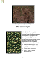
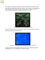
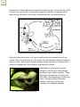
LATEBLIGHT
A Plant Disease Management
Simulation
Version 3.1
User’s Manual
Phil A. Arneson
Barr E. Ticknor
Cornell University
Cornell University
A BioQUEST Library VII Online module published by the BioQUEST Curriculum Consortium
The BioQUEST Curriculum Consortium (1986) actively supports educators interested in the
reform of undergraduate biology and engages in the collaborative development of curricula.
We encourage the use of simulations, databases, and tools to construct learning environments
where students are able to engage in activities like those of practicing scientists.
Email: [email protected]
Website: http://bioquest.org
Editorial Staff
Editor:
Managing Editor:
Associate Editors:
John R. Jungck
Ethel D. Stanley
Sam Donovan
Stephen Everse
Marion Fass
Margaret Waterman
Ethel D. Stanley
Online Editor:
Amanda Everse
Editorial Assistant: Sue Risseeuw
Beloit College
Beloit College, BioQUEST Curriculum Consortium
University of Pittsburgh
University of Vermont
Beloit College
Southeast Missouri State University
Beloit College, BioQUEST Curriculum Consortium
Beloit College, BioQUEST Curriculum Consortium
Beloit College, BioQUEST Curriculum Consortium
Editorial Board
Ken Brown University of Technology, Sydney, AU
Joyce Cadwallader St Mary of the Woods College
Eloise Carter Oxford College
Angelo Collins Knowles Science Teaching Foundation
Terry L. Derting Murray State University
Roscoe Giles Boston University
Louis Gross University of Tennessee-Knoxville
Yaffa Grossman Beloit College
Raquel Holmes Boston University
Stacey Kiser Lane Community College
Peter Lockhart Massey University, NZ
Ed Louis The University of Nottingham, UK
Claudia Neuhauser University of Minnesota
Patti Soderberg Conserve School
Daniel Udovic University of Oregon
Rama Viswanathan Beloit College
Linda Weinland Edison College
Anton Weisstein Truman University
Richard Wilson (Emeritus) Rockhurst College
William Wimsatt University of Chicago
Copyright © 1993 -2006 by Phil A. Arneson and Barr E. Ticknor. All rights reserved.
Copyright, Trademark, and License Acknowledgments
Portions of the BioQUEST Library are copyrighted by Annenberg/CPB, Apple Computer Inc., Beloit College, Claris
Corporation, Microsoft Corporation, and the authors of individually titled modules. All rights reserved. System 6,
System 7, System 8, Mac OS 8, Finder, and SimpleText are trademarks of Apple Computer, Incorporated. HyperCard
and HyperTalk, MultiFinder, QuickTime, Apple, Mac, Macintosh, Power Macintosh, LaserWriter, ImageWriter, and the
Apple logo are registered trademarks of Apple Computer, Incorporated. Claris and HyperCard Player 2.1 are
registered trademarks of Claris Corporation. Extend is a trademark of Imagine That, Incorporated. Adobe, Acrobat, and
PageMaker are trademarks of Adobe Systems Incorporated. Microsoft, Windows, MS-DOS, and Windows NT are
either registered trademarks or trademarks of Microsoft Corporation. Helvetica, Times, and Palatino are registered
trademarks of Linotype-Hell. The BioQUEST Library and BioQUEST Curriculum Consortium are trademarks of Beloit
College. Each BioQUEST module is a trademark of its respective institutions/authors. All other company and product
names are trademarks or registered trademarks of their respective owners. Portions of some modules' software were
created using Extender GrafPak™ by Invention Software Corporation. Some modules' software use the BioQUEST
Toolkit licensed from Project BioQUEST.
Lateblight is based on the work of J. A. Bruhn et al. (1987). The simulation has
been refined and adapted to the Microsoft« WindowsTM environment (ver. 3.0 or
higher) by Barr Ticknor and Phil Arneson, Department of Plant Pathology, Cornell
University.
The following files should be kept together in the same folder:
Begin Lateblight.exe - the main program
LATEBLIT.DOC - the manual
KEYHOOK.DLL - the keyhook library, which supports the context
sensitive help system.
LATEBLIT.HLP - the help file
The sample weather files:
COOLWET.LWX HOTDRY.LWX
MODDRY.LWX
MODMOD.LWX
MODWET.LWX
Sample scenario files:
CROP1.LBT
CROP2.LBT
PAST1.LBT
PAST2.LBT
PAST3.LBT
POTATO1.LBT
POTATO2.LBT
POTATO3.LBT
i
Table of Contents
WHAT IS LATE BLIGHT?..........................................................................................................1
INSTALLATION AND QUICK INSTRUCTIONS ...................................................................5
GETTING STARTED WITH LATEBLIGHT.............................................................................................6
MINI-CASE INVESTIGATIONS WITH LATEBLIGHT ..............................................................................9
PROGRAM FEATURES ............................................................................................................11
FILE MENU ..................................................................................................................................12
Run.........................................................................................................................................12
New ........................................................................................................................................12
Open.......................................................................................................................................12
Save As... ...............................................................................................................................12
Log to Disk.............................................................................................................................13
Exit.........................................................................................................................................13
POTATO MENU.............................................................................................................................13
ENVIRONMENT MENU...................................................................................................................13
Length of Season....................................................................................................................13
Emergence Date .....................................................................................................................13
Weather Report ......................................................................................................................14
INOCULUM MENU.........................................................................................................................14
Number of Sporangia.............................................................................................................14
Sources of Sporangia .............................................................................................................14
Number of Infections .............................................................................................................15
Sources of Infections..............................................................................................................15
MANAGEMENT MENU...................................................................................................................15
Spray Systemic.......................................................................................................................15
Spray Protectant... ..................................................................................................................15
Kill Vines ...............................................................................................................................16
Blitecast..................................................................................................................................16
ECONOMICS MENU .......................................................................................................................16
Costs.......................................................................................................................................16
Price .......................................................................................................................................16
Show/Hide Report..................................................................................................................16
VIEW MENU.................................................................................................................................17
Check Items............................................................................................................................17
American/Metric Measure .....................................................................................................17
Set Colors...............................................................................................................................17
Arrange...................................................................................................................................17
KEYBOARD ACTIONS....................................................................................................................19
The Main Window .................................................................................................................19
Dialog Boxes..........................................................................................................................19
The Colors Dialog..............................................................................................................20
GETTING HELP.............................................................................................................................21
TUTORIAL ..................................................................................................................................22
SAVING A STARTUP FILE ..............................................................................................................22
EFFECTS OF WEATHER..................................................................................................................22
DISEASE RESISTANCE ...................................................................................................................23
SOURCES OF INOCULUM................................................................................................................23
ii
PROTECTANT FUNGICIDE SPRAYS .................................................................................................24
SYSTEMIC FUNGICIDE SPRAYS......................................................................................................24
FUNGICIDE / WEATHER INTERACTIONS .........................................................................................24
PARTIAL RESISTANCE / FUNGICIDE INTERACTIONS ........................................................................25
ECONOMICS..................................................................................................................................25
SIDE-BY -SIDE COMPARISON OF EPIDEMICS ....................................................................................25
PRINTING OR EDITING TEXT OUTPUT ............................................................................................26
MODEL TECHNICAL DESCRIPTION...................................................................................27
TEMPERATURE EFFECTS................................................................................................................28
SPORANGIAL GERMINATION .........................................................................................................29
INFECTION....................................................................................................................................30
LESION DEVELOPMENT..................................................................................................................30
SPORULATION ..............................................................................................................................31
LESION INACTIVATION ..................................................................................................................32
DISPERSAL OF SPORANGIA ............................................................................................................32
HOST GROWTH .............................................................................................................................32
FUNGICIDE EFFECTS......................................................................................................................33
WEATHER ....................................................................................................................................34
REFERENCES.............................................................................................................................35
iii
Destroyed potatoes (Arneson 2000)
What is Late Blight?
Late blight is a disease of potatoes
caused by the fungus Phytophthora
infestans. Under favorable environmental
conditions and in the absence of any
control measures, this disease can
destroy virtually 100% of the aboveground parts of susceptible crops. Spores
produced on infected foliage can be
disseminated to the tubers, where
infections can also occur. Losses include:
•
reduction of photosynthetic area,
resulting in reduced bulking of tubers
(yield loss)
•
blighted tubers (quality loss),
•
decay of tubers in storage
(postharvest loss).
Spoiled tubers (Arneson 2000)
1
The fungus survives between seasons in lesions on the tubers. New infection may
come from new "seed" tubers that are infected, from "volunteer" tubers that were
left in the field from the previous year's harvest, and from piles of "culled" or
discarded potatoes during the grading and packing of the crop.
Early signs of late blight in the field (Arneson 2000)
The first infections, barely visible except to well trained eyes, usually are on the
sprouts emerging from infected tubers.
Sporangia of the Late Blight fungus, Phytophthora infestans (Arneson 2000)
Sporangia form by the thousands on these lesions and are disseminated by wind
and splashing rain to the developing leaf and stem tissues.
2
Germination of these spores occurs while the leaves are wet, either directly by the
formation of a germ tube or indirectly through the release of zoospores, which
swim through the water film, encyst on the leaf surface, and then germinate.
Asexual Life Cycle of the Late Blight Fungus, Phytophthora infestans
Infection takes place under cool, moist conditions by direct penetration of the
cuticle. Infection efficiency is a function of the environmental conditions and the
potato cultivar. Microscopic lesions gradually enlarge into necrotic lesions, which
continue to expand until they coalesce, blighting entire leaves.
Sporangia are produced around the
margins of the necrotic lesions during
periods of high relative humidity. These
sporangia are dispersed to initiate new
infections, thus completing the infection
cycle. During periods of favorable
weather, many such cycles occur,
resulting in an explosive epidemic.
Late season leaf damage (Arneson 2000)
3
Management of potato late blight begins by:
1.
Keeping the numbers of infected seed tubers to very low levels by
planting only certified seed potatoes
2.
Crop rotation to reduce the numbers of "volunteer" plants which may
be infected
3.
Burying or composting cull piles or at least keeping them a great
distance from the potato fields.
Control of late blight by means of potato varieties with a high degree of resistance
to P. infestans has generally proven impractical because of the rapid selection of
virulent races of the pathogen. Varieties with moderate levels of resistance,
however, have been very useful when combined with other management tactics,
particularly the use of fungicides. In most potato growing areas, regular fungicide
applications are an essential component of late blight management.
Because of environmental concerns, the problem of fungicide resistance, and the
high cost of fungicides and their application, potato growers have been forced to
reduce their overall use of fungicides and to improve the efficiency of the
fungicides they apply.
One approach has been to improve the timing and adjust the dose of fungicide
applications according to environmental conditions. Various kinds of forecasting
systems have been employed to help growers decide when and how much to spray.
By using potato varieties that are partially resistant to P. infestans, it is possible
to markedly reduce the doses and/or frequencies of fungicide sprays.
4
INSTALLATION AND QUICK INSTRUCTIONS
Lateblight will run on any system which supports Microsoft Windows
Installation
To install, insert the BioQUEST Library CD that is compatible with the Windows
operating system into the appropriate drive of your computer. Open the Online
Guide. Using the instructions on the first page of the Online Guide, navigate to the
"Lateblight" section of the Guide. Clicking on the Install button on the bottom of
the page will start the installation process. Follow the instructions on the screen.
Note: To use the Online Guide, the Acrobat Reader must be installed on your
computer. For best results, we suggest that you install Acrobat Reader version 4.0
or later. An installer for Reader version 4.0 is included on the BioQUEST Library
CD.
Quick Start
Select the "Begin Lateblight.exe" file (potato icon) or use File Run to begin your
first simulated season. A dialog box will appear asking you to choose a weather
data file. Sample weather files (with the .LWX extension) are distributed with
Lateblight. Once you open a weather file, a pair of axes will be drawn. The x-axis
represents time, and is labelled with dates. The y-axis is an arbitrary scale of 0 to
100 used to display the various inputs and results of the simulation. The View menu
allows you to choose which variables will be drawn on the graph, and shows the
units and color for each variable. The scrollbar just below the x-axis is used to
advance time. Management actions are selected from the menu system while the
season is in progress.
For more detailed information about running Lateblight, please consult the
"Lateblight Tutorial" and "Program Features" sections of this manual.
Lateblight features a help system which is accessed by pressing the <F1> key or
using the Help menu. Use the help system and this manual to learn more about the
program as you go along.
Example scenarios for Lateblight investigations are provided in the "Getting
Started with Lateblight" and the "Mini-Case Investigations with Lateblight"
sections of this manual. There is also a "Tutorial" section later in this document.
These sections are also provided separately in the "Tutorial and Activities" document.
5
Getting Started with Lateblight
First time users of Lateblight may become familiar with this program by looking at
two different seasons for growing potatoes and comparing management strategies
and the resulting losses or profits. To do this, double click the Begin Lateblight
potato icon. Go to File in the menu and choose Open. Highlight "crop1.lbt" and a
finished season will appear. Resize the window by clicking in the middle box in the
upper right or by dragging the lower right corner of the window.
Graphic output from Lateblight for Crop 1.
By choosing View, you can see what the different
color lines on the graphs represent.
6
You can add more variables in View. See Temperature (red) added below.
Choose Economics from the menu and highlight Crop Report. This shows you the
profit or the loss for the growing season. Note loss in the bottom line below.
7
Go to File in the menu and choose Open. Highlight "crop2.lbt".
If you open your Economic Report, you can see that spraying with a systemic has
resulted in a net profit under otherwise identical conditions.
8
Mini-Case Investigations with Lateblight
1. The Irish grew potatoes in Ireland for over two hundred years with good
success. In the 1840's, potato farming became far more problematic. Let's
look at the results of three different seasons in 1830 with no late blight, 1843
when the first late blight occurred in your county, and 1844.
a. Open the file "past1.lbt" and look at the results of the 1830 season.
How many potatoes can you expect to harvest?
b. Open the file "past2.lbt" and look at the results of the 1843 season. You
should note that signs of late blight infection are observed near the end of
the summer.
How many potatoes can you expect to harvest?
c. Open the file "past3.lbt" and look at the results of the 1844 season. The
agricultural methods of the day contribute to your problems. Volunteer
potatoes (tubers left in the ground over winter) were common. Also cull
piles (damaged or tubers that aren't used) are found near the growing sites
since no one suspected how this infection spread.
How many potatoes can you expect to harvest in the third season?
2. You are farming in upper state New York during the 1990's and have been
having trouble with late blight during the cool, wet weather the county has been
having for the past three years. Encouraged by a neighbor's success with a new
hybrid potato that has high resistance to late blight, you are thinking of trying
these potatoes yourself. The new seed certified potatoes will cost you about
$100 more per acre than your standard low resistance potatoes.
a. Open the file "potato1.lbt" which was created by selecting Potato and
changing resistance level from low to high and then selecting Economics and
increasing costs from $1100 to $1200 per acre.
Did you make a profit?
9
b. Unexpectedly, your region experiences a moderately dry growing season.
Open the file "potato2.lbt" which was created by running the file using
"moddry.lwx" and no other changes. Review the results.
Did you make a profit?
c. The uncertaintity of the weather raises new issues for you. You decide to
try a more vigorous spray program instead of planting the high resistance
potato. Open the file "potato3.lbt" which was created by selecting Potato
and changing resistance level from high to low and then selecting Economics
and decreasing costs from $1200 to $1100 per acre. You are spraying a
systemic every two weeks in late June until harvest. Note: When it rains,
these sprays are delayed.
Did you make a profit?
How does it compare to the use of high resistance potatoes?
What are the costs?
10
PROGRAM FEATURES
Lateblight is designed to allow you to manipulate the variables that affect the
development of the disease and to adjust the economic parameters that determine
the cost-effectiveness of the disease management procedures. You must first
select a weather data file that determines the environmental conditions under
which the simulation will execute. You can then set the characteristics of the
potato cultivar that you want to simulate--a low, moderate or high level of
resistance to P. infestans, tuber initiation occurring early, mid, or late season, and
the maximum yield potential. Next, you set the amount of initial inoculum (either
sporangia or infections or both). Finally, you can enter the production costs and
the market price for the harvested potatoes. You can save all of these start-up
values in a disk file to facilitate repeated simulations using the same initial values
for most of the parameters.
The simulation is then started, and you can progress one day at a time, one week at
a time, or you can advance the season to any desired day. During the season you
can consult the weather forecast and the Blitecast spray advisory prior to applying
a spray of either a protectant or a systemic fungicide. You can select which of the
output variables you would like to see graphed on the screen--the fungicide
residues, rainfall, daily mean temperature, hours of relative humidity above 90%,
leaf area index, latent lesions, sporangia production, percent foliage blight, and
area under the disease progress curve.
At the end of the season you can look at an economic summary of the season, and if
you wish, you can save a text summary of the season's simulation.
The following describes each of the commands in each of the menus:
11
File Menu
Run
Once you have decided on the appropriate options and parameters, select Run from
the File Menu to begin the simulated season. You will then be prompted to select a
weather data file that will provide the season's weather. To advance the progress
of the simulation during the season, use the scroll bar beneath the graph.
New
New allows you to begin a new simulation. You may repeat the same problem or
change parameters and/or options before running the new season. Any parameters
or options not changed will be the same as in the last season. You may want to use
the Save As... command before selecting New so that you can recall the current
season at a later time.
Open
Open allows you to open a saved Lateblight document in which is stored the state
of the program at the moment you executed the Save As… command in a previous
run. This includes all program options and parameter values. If the season was in
progress when the document was saved, opening it will return you to the day on
which it was saved. (This is a good way to explore and compare different
management strategies.)
Save As...
Save As creates a Lateblight document on disk using the name and extension you
provide. Use of the .LBT extension is strongly recommended to distinguish
Lateblight documents from other types of files. If you add a line for the .LBT
extension to the [extensions] section of your WIN.INI file, you will be able to
start Lateblight simply by double clicking a document. A Lateblight document
contains the complete state of the program at the time the document was saved.
If you save a document named STARTUP.LBT, Lateblight will load it automatically
when you start the program. In this way, you can override the default values
provided for the various parameters and options. A document saved before
selecting Run will contain only the program options and initial parameter values and
will take considerably less space on disk. A document saved while a season is in
progress will contain all information for that season up to the time when it was
saved.
12
Log to Disk
A plain text record of all parameter values and day-by-day simulation results can
be saved to disk using the Log to Disk... selection in the File menu. This is
especially useful for preparing printed reports. Whether you choose Log to Disk
before a season is started, in the middle of a season, or at the end of a season, the
log file will include all initial values and results from the beginning of the season
onward. If the log is closed before the end of the season, only the data up to the
day when the log was closed will be saved. A single log file can be used to record
the results of several successive seasons.
Exit
This selection terminates Lateblight. The same thing may be accomplished by
double clicking the close box in the upper left corner of the Lateblight window.
Potato Menu
Different potato cultivars can be simulated in Lateblight by altering the level of
resistance to Phytophthora infestans, the time of initiation of tuber production,
and the yield potential of the crop in the absence of disease. One of three
resistance levels--low, moderate, or high--and one of three times of tuber
initiation--early, mid, or late--can be selected. Enter the maximum yield. To
facilitate repeated simulations using the same values for the potato cultivar, the
setup conditions can be saved in a disk file using the Save As... command prior to
starting the simulation with Run.
Environment Menu
Length of Season
This variable is the number of days from median emergence of the potato vines to
harvest.
Emergence Date
This is the calendar date on which median emergence of the vines occurs. It is
used as the basis for the labeling of the x-axis.
13
Weather Report
A weather report may be requested from the Environment menu for any day of
the season. The report includes actual temperature and rainfall data from the
previous day as well as a forecast of temperature and chance of rainfall for the
current day and the next two days. As in the real world, there is a degree of
randomness in the forecasts. They are based on the weather data that will
actually be used in coming days, with a random component to reflect the inherent
difficulty of predicting the weather.
Inoculum Menu
In Lateblight there are two independent sources of inoculum--sporangia and
infections. Sporangia can be released all at once as initial inoculum or each day
during the course of the epidemic, while infections occur on the potato plants at
the time of emergence. Both Sporangia and Infections can be initialized either by
designating the Number or by selecting the Source of inoculum. Only the values in
the checked item are used, and the values in the unchecked item are ignored.
Number of Sporangia
This is one of two alternative means of setting the number of initial sporangia.
Enter the number of sporangia released per unit area. The number of sporangia
indicated will be released all at once on the day of plant emergence or each day of
the season, depending on the alternative selected. "Typical" values are 2.5 * 107
sporangia/ha as initial inoculum or 2.5 * 105 sporangia/ha each day.
Sources of Sporangia
As an alternative to setting the Number of Sporangia, you can set the quantities
of sporangia contributed by two possible sources, a cull pile (potatoes discarded
from a packing line) and a neighboring unsprayed field. To account for dispersal
losses, the distance between the field being managed and each of these inoculum
sources can be set. Enter the maximum sporangia per day released at the source.
In the case of the cull pile, the number of sporangia released each day will
decrease exponentially from this maximum as the season progresses. A "typical"
value for this maximum is 1000 sporangia/day 10 meters from the field. In the
case of the unsprayed field, the number of sporangia released per day will increase
logistically from 0.001 to 1.0 times this maximum as the season progresses. A
14
"typical" value for this maximum is 1 * 107 sporangia/ha at 10 meters from the
field.
Number of Infections
This is one of two alternative means of setting the number of initial infections.
Enter the number of infections per hectare or per acre present at plant
emergence. A "typical" value is 100 infections/ha.
Sources of Infections
There are two possible sources of initial infections, infected seed tubers and
volunteer potatoes in the field being managed. Enter the numbers of infections
per unit area present at plant emergence. A "typical" value is 100 infections/ha.
Management Menu
After the potato plants have emerged (that is, after the simulation has been
started with the Run command), the only disease management options available are
to spray a fungicide or to terminate the season early by killing the vines. There
are two general types of fungicide available. Spray Systemic... applies a fungicide
that is absorbed by the plant tissues and is therefore not subject to weathering
by subsequent rains. The systemic fungicide also acts to suppress infections that
are already established. Spray Protectant... applies a fungicide that interacts
with the fungus only on the plant surface. To be effective, it must be applied prior
to infection, and its residues must be maintained on plant surfaces by frequent
applications.
Spray Systemic...
Spray Protectant...
Enter the dose of the active ingredient in kg/hectare or lb/acre. Click on OK to
apply the fungicide on the date given at the top of the dialog box or on Cancel to
exit the dialog box without applying the spray. A warning is given if it is currently
raining. A spray applied in the rain will not leave the full residue of fungicide on
the foliage.
15
Kill Vines
The order to kill vines immediately defoliates the crop. Tuber development will
continue for seven days after defoliation.
Blitecast
The Blitecast forecasting system (Krause, et al., 1975) sums the "rain-favorable"
days and blight severity values for the past week and makes a spray
recommendation for the current day. The decision whether or not to use the
Blitecast system is indicated by checking the appropriate item at the bottom of
the Management menu prior to the beginning of the season (before selecting Run).
If you decide to use Blitecast, you will be charged for the service at the end of
the season, even if you never request a Blitecast report. A report is requested
during the season by selecting the Blitecast menu item. This item will be present
only if Blitecast is being used.
Economics Menu
The costs and revenues of the potato field being managed can be established
before the start of the season (before Run is selected) by selecting Costs... or
Price.... At the end of the season a full accounting can be displayed with Show
Report.
Costs
For each of the items, enter the cost per acre or per hectare. When all of the
items show the desired values, click OK.
Price
Enter the market price per cwt. or per kg. for the current season's potato crop
and click on OK.
Show/Hide Report
The economic report is available at the end of the season (when the simulation has
terminated). It is invoked from the Economics menu. Exit the economic report by
double clicking the close box in the upper left corner of the window, or by
selecting Hide Report from the menu.
16
View Menu
Check Items
The View menu allows you to select which of the simulation variables will be
displayed on the graph as the season progresses. A checked variable will be
represented by a line of the same color as the check mark. In this way, the View
menu doubles as a legend for the graph. In addition, the View menu also shows the
current scaling factors for all variables.
American/Metric Measure
The American Measure and Metric Measure check items in the View Menu allow
you to choose which system of units will be used throughout the program. The
American system expresses distances in feet and inches, areas in acres, weights in
pounds (lbs.) or hundredweight (cwt., 100 lbs.), and temperatures in degrees
Fahrenheit. The metric system expresses distances in meters, areas in hectares,
weights in kilograms, and temperatures in degrees Centigrade. Whichever system
of measurement you choose will be used consistently in all dialog boxes and other
program displays.
Set Colors
The Set Colors command allows you to change the colors that are used to
represent the various simulation variables on the Lateblight graph. In this way,
you can be sure the different lines on the graph are readily distinguishable,
regardless of what combination of variables you choose to display. The Color
Choices dialog box shows all of the variables that can be displayed on the graph,
along with their currently assigned colors. When the radio button next to a
variable is checked, the color for that variable can be changed by clicking on the
new color in the palette at the bottom of the dialog. The line next to the variable
name will change color immediately to reflect your choice. When a variable is
checked in the View menu, indicating that it is to be drawn on the graph, the check
mark will be the same color as that variable's line on the graph.
Arrange
One of the benefits of the Microsoft Windows environment for a program such as
Lateblight is that it allows multiple copies (or "instances") of a program to be run
17
simultaneously. In this way, it is possible to do side-by-side comparisons with each
instance of Lateblight simulating a different situation. The arrange command is
intended to be used when more than one instance of Lateblight is running.
Selecting this command from the View menu will cause all non-iconic Lateblight
windows to be arranged side-by-side to use the full screen without overlapping.
This command will arrange any number of Lateblight windows, but is really only
practical with three or fewer. If there are more than three Lateblight windows to
be arranged, each gets only a very narrow slice of the display, making viewing very
difficult. Note that instances of Lateblight which have been minimized and are
represented only by icons will not be arranged.
18
Keyboard Actions
Like most Microsoft Windows applications, Lateblight is designed to use a mouse.
Although a mouse is strongly recommended, it is not essential. A keyboard
interface has been provided for all of the essential features of the program. Even
when a mouse is present, there may be times when the keyboard interface is more
convenient for certain actions. Wherever possible, we have used the keystrokes
that are standard among Windows applications. The following is a brief summary
of the keyboard interface of Lateblight.
The Main Window
The menu system uses the standard Windows keystrokes; underlined letters in
menu items represent hot keys. The <Alt> key followed by the appropriate hot key
provides access to a popdown menu. For example, <Alt>, F causes the File menu to
pop down. The arrow keys move the highlight to different items within the menu.
Pressing <Enter> with a menu item highlighted is the same as selecting that menu
item with the mouse. Pressing the hot key for a menu item has the same effect.
While the File menu is pulled down, pressing 'O' invokes the Open dialog box.
The window scroll bars also use the standard keystrokes. <PgUp> and <PgDn>
operate the vertical scroll bar, while <Ctrl>+<PgUp> and <Ctrl>+<PgDn> operate the
horizontal scrollbar. Note the distinction between the horizontal window scroll,
which appears at the very bottom of the window when it is displaying a graph that
is wider than the window, and the simulation scrollbar, which appears below the xaxis when a season is in progress and is used to advance the date. The simulation
scrollbar uses the <+> key to advance one day, or <Ctrl>+<+> to advance one week.
<End> is equivalent to dragging the thumb all the way to the right, and advances the
simulation to the end of the season.
Dialog Boxes
<Enter> and <Esc> operate the "OK" and "Cancel" buttons, respectively. The <Tab>
key shifts the input focus from one control to the next. The control with the input
focus is the one that will respond to keyboard actions (other than <Enter> or
<Esc>). The input focus is indicated by highlighting of the text in an edit control,
or a dotted rectangle around a radio button. When a radio button has the input
focus, the spacebar toggles its status. If the button is one of a mutually exclusive
group, when it is deselected, the next button in the group will automatically be
selected.
19
The Colors Dialog
The Colors dialog box allows you to reassign the colors that are used to represent
the various simulation variables on the graph. It is a little different from most of
the other dialog boxes. <Tab> cycles among the currently selected radio button,
the color palette, the OK button and the Cancel button. When the input focus is
on a radio button, the spacebar or the arrow keys can be used to select a different
button. When the input focus is in the color palette, it is represented by an
inverted rectangle on the current color button. The focus is moved from one color
button to the next by using the arrow keys. Pressing the spacebar while the input
focus is on a color button has the same effect as clicking that color with the
mouse; that color is assigned to the variable whose radio button is selected.
20
Getting Help
Lateblight features a context sensitive help system which provides information
about all aspects of the program, To access the help system, press <F1>. This will
take you directly to the help item most appropriate for your current situation. If
no specific help item exists you will be presented with the help index. Selecting
Index from the Help Menu will take you directly to the help index.
To get help on a menu command, pull down the menu and highlight the command
using either the mouse or the arrow keys. While the command is still highlighted
(don't let up on the mouse button!), press <F1>. The Help window will appear with
the appropriate information. To get help while in a dialog box. press <F1>.
If you need more general help with the Microsoft Windows « environment, use the
Help Menu in either the Program Manager or File Manager window. To learn more
about the help system, press <F1> while the Help window is active, or select Using
Help from the Help window's Help menu.
21
TUTORIAL
This tutorial assumes that you are already acquainted with Microsoft Windows.
Therefore, our instructions will focus on the simulation and the features unique to
Lateblight. If you need help with the Windows environment itself, go to the Help
menu of either the Program Manager or the File Manager. The information
presented there explains the standard features of the environment. The
exercises suggested here represent only a small fraction of the versatility of
Lateblight and the ways in which it can be used to explore epidemiological concepts.
In addition to the structured exercises such as these, we encourage you to ask
your own questions and run the simulations necessary to answer them.
Saving a Startup File
When you start Lateblight for the first time, all program options and parameters
will be set to the default values that are written into the program. After running a
season with different values for some options or parameters, you will want to
restore the original values. To make this easier, you will now save the default
values in a disk file. Select Save As... from the File menu. When the dialog box
appears, prompting you for a file name, enter STARTUP.LBT, and click OK. When
Lateblight is started, it will look for this file and load it automatically if found.
You can also load it from the File menu by selecting Open... . In addition to
providing a convenient means of restoring the default values without having to
restart the program, this mechanism allows you to change default values. The
options and values that are in effect when STARTUP.LBT is saved will become the
new defaults.
Effects of Weather
Select Run from the File menu. A dialog box will appear prompting you to open a
weather data file. Open the file COOLWET.LWX. Once the weather data are
loaded, a pair of axes will appear, with calendar days along the x-axis and a scale
ranging from 0 to 100 as the y-axis. Advance the simulation to the end of the
season by pressing the <End> key on the keyboard. The three curves that appear
represent the leaf area index, the percent blighted foliage, and the area under the
disease progress curve (AUDPC). Note the date on which the percent blight
reaches 50 by placing the tip of the arrow cursor approximately at the 50% point
on the curve and pressing the left mouse button. Hold the button down and move
the arrow along the curve until Y = 50. Similarly move the arrow to the end of the
AUDPC curve and note the final AUDPC.
22
To save this graph (actually the complete state of the program at this point) in a
disk file, select Save As... from the File menu and enter COOLWET.LBT as the
file name. Save the text output in a disk file by selecting Log to disk... from the
File menu and entering the name COOLWET.TXT. The log file will remain open to
record more than one run of the simulation. You must close it by selecting Close
Log File from the File menu.
Select File, New and Run, and repeat the above sequence with the weather data
sets MODMOD.LWX (moderate temperatures and moderate rainfall) and then
HOTDRY.LWX. Note the date on which 50% blight occurs and the final AUDPC as
before.
Disease Resistance
Partial or rate-reducing resistance to Phytophthora infestans plays an important
role in late blight management, despite the fact that it does not completely
prevent infection. To observe the effect of this resistance alone on a late blight
epidemic, check Resistance Level, Low in the Potato menu and run the simulation
using the MODMOD.LWX weather data set. Consider this the susceptible check
against which you will compare Resistance Level, Moderate and Resistance Level,
High. As before, save your graphic output with Save As..., using the file names,
"RESISLOW.LBT", "RESISMOD.LBT", and "RESISHI.LBT", and/or save text
output with Log to disk..., using the same file names with the extension ".TXT".
Do not forget to close the log file! When you are finished with this exercise,
restore the default values by opening STARTUP.LBT.
Sources of Inoculum
As with real epidemics, the initial inoculum in Lateblight can be introduced as
sporangia or lesions or both. The source of sporangia can be piles of cull potatoes
from the packinghouse or a nearby unsprayed field of potatoes. The source of
sporulating lesions can be infected seed tubers, which give rise to infected plants,
or volunteer potatoes from the previous year's crop, a portion of which also gives
rise to infected plants. Select Sporangia, Sources... from the Inoculum menu and
set the maximum number of sporangia per day coming from a cull pile 10 meters
from the field to 5000. (The number of sporangia coming from an adjacent
unsprayed field should be zero.) Run the simulation using the MODMOD.LWX
weather file, and note the date of 50% blight and the final AUDPC. Select New
from the File menu and this time run the simulation with the cull pile 20 meters
from the field, recording the date of 50% blight and the final AUDPC as before.
23
Repeat the simulation using 40 and 80 meters as the distance from the cull pile to
the field.
Protectant Fungicide Sprays
The weather data files included with Lateblight have been modified to facilitate
studies of regular spray schedules. No rain will occur on intervals of 5 or 7 days,
starting on either day 15 or day 50 after emergence (June 15 or July 20, if
emergence is set at June 1). Reset the starting conditions by opening
STARTUP.LBT. Use the MODMOD.LWX weather data file, and advance the season
to July 20 by dragging the thumb on the scroll bar or by clicking on a combination
of pageup (advance one week at a time) or the right arrow (advance one day at a
time). Since this will be the starting date for all our sprays, it will be handy to
save the simulation at this point for starting all the subsequent simulations. Select
Save As... from the File menu, and name the file SPRSTART.LBT. Select Spray
Protectant... from the Management menu and apply the fungicide at the default
dose of 1.25 kg/ha. Advance the simulation 5 days, and repeat the protectant
spray. Spray the protectant every 5 days for a total of 14 sprays, and determine
the final percent blight at the end of the season.
Open SPRSTART.LBT again to start a new season, and spray the protectant every
7 days for a total of 10 sprays. Repeat using 7 protectant sprays at 10-day
intervals, and again with 5 protectant sprays at 14-day intervals.
Systemic Fungicide Sprays
Restart the simulation by opening the SPRSTART.LBT file that you created for the
protectant fungicide sprays. Select Spray Systemic... and apply the fungicide at
the default dose of 0.22 kg/ha. Apply a total of 3 sprays at 3-week intervals, and
determine the final percent blight.
Fungicide / Weather Interactions
In addition to providing longer periods of leaf wetness for the development of the
fungus, rain reduces the effectiveness of the fungicide by removing the protective
residues on the foliage. Restart the program with STARTUP.LBT, and use the
MODWET.LWX weather data file. Spray the protectant, beginning on July 20 and
continuing at 7-day intervals for a total of 10 sprays. Compare the final percent
blight with that of the same spray schedule using the MODMOD.LWX weather
data set. Now restart the simulation using the MODDRY.LWX weather data set.
24
Compare the results of the 7-day and 10-day spray intervals with those of the
corresponding spray schedules using the MODMOD.LWX weather.
Partial Resistance / Fungicide Interactions
While a moderate level of resistance alone may not provide adequate control of
late blight, it will markedly reduce the number of fungicide sprays required to
control the disease. Review the results for the unsprayed epidemics on the potato
cultivars with a low level of resistance and a moderate level of resistance. (This
can be done by opening previously saved *.LBT files or by using a text editor to
review the *.TXT files previously logged to disk.) Compare the results of epidemics
where the protectant fungicide was applied at 5- and at 7-day intervals on the low
resistance potato cultivar with those where the protectant was applied at 10- and
14-day intervals on the moderately resistant cultivar.
Economics
In Lateblight, it is possible to compare the costs and benefits of various spray
options by entering the appropriate values under the Costs... and Price... items in
the Economics menu. These menu items are available only at the start of the
simulation, and the Show Report menu item is available only at the end of the
season. Either using your own values or the default values for the costs and price,
compare the costs and revenue of the following potato cultivar / spray schedule
combinations:
(1) Low resistance, Protectant, 7-day intervals
(2) Moderate resistance, Protectant, 14-day intervals; and
(3) Low resistance, Systemic, 21-day intervals.
Side-by-side Comparison of Epidemics
Open the MODMOD.LBT file that you saved earlier. Temporarily reduce this copy
of Lateblight to an icon. To do this click on the small, downward-pointing triangle
in the upper right corner of the window. (Notice that the icon displays the name
of the file you opened) Start another copy of Lateblight and open COOLWET.LBT,
which you saved earlier. Double click on the icon displaying MODMOD.LBT to
restore it to a normal sized window. Now, with both instances of Lateblight
running simultaneously, select Arrange from the View menu of either instance.
This will rearrange both instances so that each occupies half of the screen. Notice
that there is a scroll bar for each window as well as a (now nonfunctional) scrollbar
for each graph. Click in the pageup area (the grey part) of each window scrollbar
to move to the end of each graph. Side-by-side comparison of the graphic output
is now possible.
25
Printing or Editing Text Output
The output saved with Log to Disk... is a plain text file, which can be edited
and/or printed with any word processing program including Windows Notepad and
Windows Write. The text is formatted for a fixed pitch font such as Courier, and
uses the ANSI character set. You can edit the saved text without exiting from
Lateblight; just be sure the log file is closed from Lateblight's File menu before
editing it with another program.
26
MODEL Technical DESCRIPTION
This version of Lateblight was adapted from the simulation originally written by J.
A. Bruhn et al. (1980) and modified in various ways over the years by different
people working in the research program of W. E. Fry, Department of Plant
Pathology, Cornell University. We have attempted to retain as much as possible
the original structure of the model, but some small modifications have been
necessary to enhance its pedagogical value. While the simulation is sufficiently
realistic for teaching purposes, this version should not be trusted as a research
tool or a management decision making aid.
In order to make Lateblight respond as realistically as possible to environmental
and management variables, the development of the fungus is simulated
mechanistically, closely following the P. infestans life cycle. The model's state
variables represent the major morphological stages in the fungus development:
Sporangia (landed on susceptible sites)
Zoospores (following indirect germination)
Germinated sporangia
Germinated zoospores
Latent lesions
Sporulating, expanding lesions
Sporulating, inactive lesions (not expanding)
Inactive lesions (nonsporulating, necrotic tissue)
Sporangia available for dispersal
Dispersed sporangia
The model's transfer functions describe different developmental processes:
Indirect germination
Direct germination
Infection
Lesion expansion
Sporulation
Lesion inactivation (cessation of expansion)
Necrosis (cessation of sporulation)
Dispersal of sporangia
Catch of sporangia
The model operates on a daily time step.
27
Temperature Effects
The effect of temperature on disease development is simulated independently for
each of six different developmental processes using polynomial equations (Table 1).
Table 1. Rates of Pathogen Development as a Function of Temperature (_C ).
Temperature
Effect
Direct Germination
Range
Min Max
Equation
TempEffDirect = 2.1
- 0.48 TempLeafWet
+ 0.031 TempLeafWet2
- 0.00045 TempLeafWet3
- 4.5 10-6 TempLeafWet4
14
29
Indirect Germination TempEffIndir = 0.0134
+ 0.0698 TempLeafWet
+ 0.0185 TempLeafWet2
- 0.00223 TempLeafWet3
+ 7.48 10-5 TempLeafWet4
- 7.68 10 -7 TempLeafWet5
0
24
Zoospore Germination TempEffZoosp = 0.00494
+ 0.364 TempLeafWet
- 0.05813 TempLeafWet2
+ 0.00452 TempLeafWet3
- 1.617 10-4 TempLeafWet4
+ 2.068 10-6 TempLeafWet5
0
28
Infection
TempEffInfec = 0.4846
+ 0.3735 TempHumid90
- 0.03556 TempHumid902
+ 0.001509 TempHumid903
- 2.405 10 -5 TempHumid904
1.5
30
Lesion Expansion
TempEffLesEx = sqrt (8.4 10-4
+ 0.1261 DailyMeanTemp
- 0.03079 DailyMeanTemp2
+ 0.00308 DailyMeanTemp3
- 1.152 10-4 DailyMeanTemp4
+ 1.414 10-6 DailyMeanTemp5)
28
0
33
Sporulation
TempEffSporu = - 0.3882
+ 0.2482 TempHumid90
- 0.03817 TempHumid90 2
+ 0.00252 TempHumid903
- 5.32 10 -5 TempHumid904
0
26
Parameters of the polynomial equations were estimated by multiple regression using the data of
Crosier (1934).
Sporangial Germination
Sporangia germinate by two pathways, direct and indirect, depending on the
ambient temperature during the period of leaf wetness: (See Table 1.)
GermSporangia = LandedSporangia * (DIRMAX * TempEffDirect)
Zoospores = LandedSporangia * (INDMAX * ZSPR * TempEffIndir)
where
DIRMAX = 0.29 sporangia/day,
INDMAX = 0.81 sporangia/day, and
ZSPR = 6.567 zoopores/sporangium
(Marks, 1965; Ullrich and Schober, 1972; Warren and Calhoun, 1975).
The temperature effect is determined by the appropriate polynomial function in
Table 1.
The zoospores germinate only while the leaves are wet and in response to the mean
temperature during the period of leaf wetness:
GermZoospores = Zoospores * ZOOMAX * TempEffZoosp
where
ZOOMAX = 0.96 zoospores/day.
29
Infection
Infection efficiency is a function of leaf wetness, mean temperature during the
period of leaf wetness, the susceptibility of the potato cultivar, the type of
fungicide and its residue level, and the amount of uninfected tissue remaining.
LatentInfections = (INFMAX_SP * GermSporangia + INFMAX_ZSP * GermZoospores) *
TempEffInfec * LeafWetEff * Susceptibility * FungicideEffect * (1.0 - BlightProportion)
where
INFMAX_SP = 0.1 infections/germinated sporangium/day and
INFMAX_ZSP = 0.01 infections/germinated zoospore/day
(Lapwood and McKee, 1966). The temperature effect is determined by the
appropriate polynomial function in Table 1. Maximum infection efficiency occurs at
21_C with 24 hours of leaf wetness, but the effects of temperature on infection
efficiency are small between 10_ and 22_C. No infections occur below 1.5_C or
above 30_C (Crosier, 1934). Infection occurs only if the leaves are wet. The
susceptibility factors for the susceptible, moderately resistant, and resistant
cultivars are 1.0, 0.9, and 0.8, respectively. The protectant and systemic
fungicides have different dose responses, the systemic requiring a lower residue
to achieve the same effect. (See "Fungicide effects" below.)
Lesion development
Lesions are divided into four types:
Latent lesions
Sporulating, expanding lesions
Sporulating, inactive lesions (not expanding)
Inactive lesions (nonsporulating, necrotic tissue)
All successful infections produce latent lesions. The latent periods for the
susceptible, moderately resistant, and resistant cultivars are 6, 6, and 7 days,
respectively. At the end of the latent period, the lesion diameter is set at 2 mm,
following which the sporulating lesions expand for four days:
LesionDiam[age] = LesionDiam[age-1] + (MAXLES * TempEffLesEx * LesionExp * IncrFact *
FungicideFact * (1.0 - BlightProportion))
30
where
(Guzman-N, 1964; Lapwood, 1961)
the temperature effect is determined by the appropriate polynomial function in
Table 1
LesionExp is 1.5, 1.4, and 1.4 for the susceptible, moderately resistant, and
resistant cultivars, respectively
IncrFact is a factor that decreases linearly from 1.0 to 0.0 over the five days
following the latent period, and
FungicideFact is a factor between zero and one calculated from the dose
response of the fungicide. (See "Fungicide effects" below.)
MAXLES = 4.35 mm/day
The total lesion area assumes circular lesions:
LesionArea[age] = LesionNumber[age] * (LesionDiam[age] / 2)2 * p
In the original model, the numbers of lesions of each age were passed daily into the
next age class:
LesionNumber[age] = LesionNumber[age-1]
In the current version of the model, this has been modified to pass a proportion of
the lesions in each class on to the next age class each day:
LesionNumber[age] = LesionNumber[age] + LesionNumber[age-1] * TRANSFER
LesionNumber[age-1] = LesionNumber[age-1] - LesionNumber[age-1] * TRANSFER
where
TRANSFER = 0.38 (essentially a "tuning parameter", adjusted so that the model's output gave a
good fit to disease progress observed in the field trials in 1977 and 1978 near Freeville,
NY.)
Sporulation
Sporulation occurs on lesions from the end of the latent period until they are 14
days old:
AttachedSporangia = SPRMAX * SporulationFct * TempEffSporu * HumidityFct *
SysFungicideFct * TotalLesionArea * (1.0 - BlightProportion)
where
SPRMAX = 763.2 (Lapwood, 1961)
31
SporulationFct is 0.55, 0.45, and 0.45 for the susceptible, moderately resistant, and resistant
cultivars, respectively, and
the temperature effect is determined by the appropriate polynomial function in Table 1.
Sporulation occurs only if the relative humidity is above 90% (DeWeille, 1963).
The effect of the systemic fungicide on sporulation is determined by the dose
response discussed below.
Lesion inactivation
On the fifteenth day following its initiation, a lesion ceases sporulation and its area
is added to the inactive lesion area, which is added to the total blighted area when
calculating the blight proportion. All lesions become inactive if the daily mean
temperature exceeds 41_C for three consecutive days (Wallin and Hoyman, 1958).
Dispersal of sporangia
No attempt has been made in Lateblight to simulate the biophysical mechanisms of
dispersal of sporangia. All of the spores that are produced are dispersed, but the
proportion of sporangia surviving are first adjusted for temperature dependent
mortality:
if (DailyMeanTemp > 21.0)
SporeSurvival = e (6.0 * (-0.0256 * DailyMeanTemp + 0.537))
else
SporeSurvival = 1.0
The number of sporangia landing on susceptible sites (and thus available for
infection) depends on the amount of foliage present:
LandedSporangia = AttachedSporangia * SporeSurvival * 0.025 * min (LeafAreaIndex / 3.5,
1.0)
Host growth
The increase in leaf area index is linear up to the day determined by the
characteristics of the cultivar (early-, mid-, or late-season) and reaches a
maximum, also characteristic of the cultivar:
32
Early Mid Late
Day foliage growth stops
44
52
59
Maximum leaf area index
2.5
3.5
4.5
Tuber production is a function of temperature, cultivar, and time. Tuber initiation
can occur above 0_C and below 30_C. A temperature factor for tuber initiation is
generated by the quadratic:
TuberInitFact = - 0.00911 + 0.1038 Temp - 0.00296 Temp2
Physiological time is then accumulated at a rate that depends on the cultivar:
TuberInitTime = TuberInitTime + CvTuberFact * TuberInitFact
where
CvTuberFact is 1.600, 1.404, and 1.333 for the early-, mid-, and late-season cultivars,
respectively.
Tuber production is initiated when 45 physiological time units have accumulated.
The rate of tuber production is also a quadratic function of temperature:
TuberProdFact = - 0.3837 + 0.1261 Temp - 0.00298 Temp2
Again physiological time is accumulated for the production of tubers:
TuberProdTime = TuberProdTime + CvTuberFact * TuberProdFact
The production of tubers in tons/hectare is then:
Tubers = 0.56 * TuberProdTime
Fungicide effects
The protectant fungicide effect was modified from that of earlier versions of the
model, where the average effect was calculated from the individual effects of the
fungicide residues distributed among four levels in the canopy according to a
gamma distribution (Bruhn and Fry, 1982). There is no longer an effect of canopy
level -- only an average response simulated with a linear, probit / log dose function:
ProbitResponse = 5.0 + ProbitSlope * log10 (AverageResidue / LD50)
33
The proportional effect is simulated with a logistic function that approximates the
probit function and is exactly equal at 0.01, 0.50, and 0.99.
The details of the simulation of the systemic fungicide effects are described by
Milgroom et al. (1988). The only effect of the protectant fungicide is the
inhibition of infection (Bruhn and Fry, 1981), whereas the systemic fungicide not
only inhibits infection but also reduces the rate of lesion expansion and inhibits
sporulation (Milgroom and Fry, 1988).
Weather
The following environmental variables are read from an external weather data file:
Rainfall:
Daily rainfall in inches
DailyMeanTemp: Daily mean temperature (_C)
Humid90Hours:
Hours per day of relative humidity above 90%
TempHumid90: Mean temperature (_C) during the above humid period
In addition, two environmental variables are approximated with the following
calculations:
LeafWetHours = Humid90Hours + 3.0
TempLeafWet = DailyMeanTemp + TempHumid90) / 2.0
34
REFERENCES
Bruhn, J. A., R. I. Bruck, W. E. Fry, P. A. Arneson, and E. V. Keokosky. 1980. Lateblight: A Disease
Management Game. Computer program and manual, Department of Plant Pathology. Cornell
University, Ithaca, NY.
Bruhn, J. A. and W. E. Fry. 1981. Analysis of potato late blight epidemiology by simulation modeling.
Phytopathology 71:612-616.
Bruhn, J. A. and W. E. Fry. 1982. A mathematical model of the spatial and temporal dynamics of
chlorothalonil residues on potato foliage. Phytopathology 72:1306-1312.
Crosier, W. 1934. Studies in the biology of Phytophthora infestans (Mont.) DeBary. Memoir 155.
Cornell University Agricultural Experiment Station. March 1934. 37 pp.
DeWeille, G. A. 1963. Laboratory results regarding potato late blight and their significance in the
epidemiology of blight. Eur. Potato Jour. 6:121-130.
Glendinning, D. R., J. A. MacDonald and J. Grainger. 1963. Factors affecting the germination of
sporangia of Phytophthora infestans. Trans. Brit. Mycol. Soc. 45:595-603.
Guzman-N., J. 1964. Nature of partial resistance of certain clones of three Solanum species to
Phytophthora infestans. Phytopathology 54:1398-1404.
Lapwood, D. H. 1961. Potato haulm resistance to Phytophthora infestans. II. Lesion production and
sporulation. Ann. Appl. Biol. 49:316-330.
Lapwood, D. H. and R. K. McKee. 1966. Dose-response relationships for infection of potato leaves
by zoospores of Phytophthora infestans. Trans. Brit. Mycol. Soc. 49:679-686.
Marks, G. E. 1965. The cytology of Phytophthora infestans. Chromosoma 16:681- 692.
Melhus, I. E. 1915. Germination and infection with the fungus of the late blight of potato
( Phytophthora infestans). Wisc. Agr. Exp. Sta. REs. Bull. 37:1-64.
Milgroom, M. G., C. E. McCulloch, and W. E. Fry. 1988 Distribution and temporal dynamics of
metalaxyl in potato foliage. Phytopathology 78:555-559.
Milgroom, M. G. and W. E. Fry. 1988. A model for the effects of metalaxyl on potato late blight
epidemics. Phytopathology 78:559-565.
Ullrich, J. and B. Schoger. 1972. Zoosporenzahl und Sporangiengrube bei Phytophthora infestans
(Mont.) DeBary. Phytopath. Z. 74:268-271.
Waggoner, P. E. and J. G. Horsfall. 1969. EPIDEM: a simulator of plant disease written for a
computer. Bull. Conn. Agr. Exp. Sta., New Haven, No. 698. 80 pp.
35
Wallin, J. R. and W. G. Hoyman. 1958. Influence of post-inoculum air temperature maxima on
survival of Phytophthora infestans on potato leaves. Amer. Potato Jour. 35:769-773.
Warren, R. C. and J. Calhoun. 1975. Viability of sporangia of Phytophthora infestans in relation to
drying. Trans. Brit. Mycol. Soc. 64:73-78.
36