Download Module 1: Relations

Principles of Mathematics 12
Contents
1
Module 1: Relations
Section 1:
Section 2:
Module 1:
Review of Mathematics 11
Lesson 1
Graphing Calculator Review
5
Lesson 2
Functions and Interval Notation
15
Lesson 3
Inverse Functions
24
Lesson 4
Polynomial Functions and Their Graphs
31
Review
45
Section Assignment 1.1
47
Transformations
Lesson 1
Translations
59
Lesson 2
Reflections
69
Lesson 3
Absolute Value Functions
81
Lesson 4
Stretches and Compressions
89
Lesson 5
Reciprocal Relations
103
Lesson 6
Composition of Transformations
113
Summary
121
Review
123
Section Assignment 1.2
127
Answer Key
137
Module 1
2
Module 1
Contents
Principles of Mathematics 12
Principles of Mathematics 12
Section 1, Introduction
3
Module 1, Section 1
Review of Mathematics 11
Introduction
In this section you will review a number of the concepts and
processes encountered at the end of Principles of Math 11. Most of
these concepts deal with functions and coordinate geometry. A solid
foundation of polynomials and rational functions is necessary to
master transformations, which you will encounter in Sections 2
and 3 of this module and also in Modules 2 and 3.
Section 1 — Outline
Lesson 1
Graphing Calculator Review
Lesson 2
Functions and Interval Notation
Lesson 3
Inverse Functions
Lesson 4
Polynomial Functions and Their Graphs
Review
Module 1
4
Notes
Module 1
Section 1, Introduction
Principles of Mathematics 12
Principles of Mathematics 12
Section 1, Lesson 1
5
Lesson 1
GRAPHING CALCULATOR REVIEW
Outcomes
Upon completing this lesson, you will be able to carry out these
operations on a graphing calculator:
• Enter and edit polynomial equations
• Graph the equations and adjust the viewing window
• Solve the equations
Overview
If you used a graphing calculator for Principles of Math 11, then
consider this lesson optional. You should do just a few of the
exercises to make sure you remember how the graphing and solving
functions work.
The directions here are specific to the TI-83 or TI-83Plus models
from Texas Instruments. You may be using a different TI model, or
one made by Hewlett-Packard, Sharp, Casio, or another
manufacturer. Any graphing calculator will get you through the
provincial exam (except the HP-48, which is not allowed). But if you
use another brand of calculator, you will need to refer to its user
manual to find out how to do what these instructions tell you.
Module 1
6
algebraic solution. This means you can use your calculator, but
you need to provide a solution without the use of the “graphing”
tool on your calculator.
Section 1, Lesson 1
Principles of Mathematics 12
6
Section 1, Lesson 1
Principles of Mathematics 12
Q:
Q: Can
Can II use
use an
an ordinary
ordinary scientific
scientific calculator
calculator for
for the
the exams
exams in
in this
this
course
and
for
the
Provincial
exam?
course and for the Provincial exam?
Solving Polynomial Equations Using the Graphing Calculator
A:
Not
You
are
bring
one
ifif you
A: have
Not much.
much.
Youconsiderable
are allowed
allowed to
to
bring
one to
to exams
exams
you want
want to,
to,
You
developed
skill
at finding
the rational
(which
but
it’s
calculator
you
bring
Provincial
but integral)
it’s not
not enough.
enough.
The
calculator
you equations.
bring to
to the
the
Provincial
includes
roots ofThe
given
polynomial
But
the roots
exam
must
be
able
to
display
graphs
in
its
display
window,
exam mustequation
be able to
display
graphs inrational.
its display
window,
as
of a polynomial
are
not necessarily
They
mightas
well
as
solve
(calculate
and
display
the
roots
of)
equations.
well
as
solve
(calculate
and
display
the
roots
of)
equations.
well be irrational numbers (non-periodic non-terminating decimals).
This possibility
can makeaathe
algebraic
solutionby
of the
the
equation
You
graphing
calculator
You can
can distinguish
distinguish
graphing
calculator
by
the size
size of
of its
itsvery
tedious.
The window.
graphing
calculator
can
simplify the
process.
display
graphing
calculators
have
aa large
display
window. All
All
graphing
calculators
have
large (for
(for aa
calculator)
rectangular
display:
about
cm
high
66 cm
calculator)
rectangular
display:
about 44and
cmfollow
high by
by
cm wide.
wide. If
If
A word
of caution
as we begin:
enter values
the
steps
your
display
is
than
cm
your
calculator’s
display
is less
lesshas
than
cm high,
high, it
it won’t
won’t
work for
for
slowly
andcalculator’s
carefully. The
calculator
no33tolerance
for
entrywork
the
exam.
the
provincial
exam.
errors,
noprovincial
matter how
small.
The
The graphing
graphing calculator
calculator also
also includes
includes all
all the
the functions
functions of
of aa
Also, negative numbers must be signed using the negation (-)
scientific
scientific calculator.
calculator. While
While you
you may
may bring
bring two
two calculators
calculators to
to
exams
exams (one
(one scientific,
scientific, one
one graphing),
graphing), most
most students
students find
find that
that the
the
Module 1
graphing
graphing calculator
calculator is
is the
the only
only one
one they
they need.
need.
Q:
Q: Do
Do II still
still need
need to
to be
be able
able to
to solve
solve equations
equations by
by algebra,
algebra, i.e.,
i.e., by
by
other
other methods
methods II have
have been
been taught
taught that
that do
do not
not use
use aa calculator?
calculator?
A:
A: Yes!
Yes! The
The Provincial
Provincial Exam
Exam has
has three
three sections.
sections. The
The first
first section
section is
is
multiple
choice
and
you
are
not
allowed
to
use
a
calculator.
In
multiple choice and you are not allowed to use a calculator. In
section
section two,
two, the
the second
second multiple
multiple choice
choice section,
section, you
you are
are free
free to
to
use
use your
your graphing
graphing calculator.
calculator. The
The third
third section
section is
is aa long
long answer
answer
section
section and
and includes
includes questions
questions that
that specifically
specifically ask
ask for
for an
an
algebraic
solution.
This
means
you
can
use
your
calculator,
algebraic solution. This means you can use your calculator, but
but
you
you need
need to
to provide
provide aa solution
solution without
without the
the use
use of
of the
the “graphing”
“graphing”
tool
tool on
on your
your calculator.
calculator.
Solving
Solving Polynomial
Polynomial Equations
Equations Using
Using the
the Graphing
Graphing Calculator
Calculator
You
You have
have developed
developed considerable
considerable skill
skill at
at finding
finding the
the rational
rational (which
(which
includes
includes integral)
integral) roots
roots of
of given
given polynomial
polynomial equations.
equations. But
But the
the roots
roots
of
of aa polynomial
polynomial equation
equation are
are not
not necessarily
necessarily rational.
rational. They
They might
might
well
well be
be irrational
irrational numbers
numbers (non-periodic
(non-periodic non-terminating
non-terminating decimals).
decimals).
This
This possibility
possibility can
can make
make the
the algebraic
algebraic solution
solution of
of the
the equation
equation very
very
tedious.
tedious. The
The graphing
graphing calculator
calculator can
can simplify
simplify the
the process.
process.
A
A word
word of
of caution
caution as
as we
we begin:
begin: enter
enter values
values and
and follow
follow the
the steps
steps
slowly
slowly and
and carefully.
carefully. The
The calculator
calculator has
has no
no tolerance
tolerance for
for entry
entry
errors,
errors, no
no matter
matter how
how small.
small.
(-)
Also,
Also, negative
negative numbers
numbers must
must be
be signed
signed using
using the
the negation
negation (-)
Module
Module 11
Principles of Mathematics 12
Section 1, Lesson 1
7
button just to the left of the ENTER button, not the subtract −
operation button; otherwise you’ll get a “syntax error” message. (On
other brands of calculators, the (-) key may be a ± or ± /− key.)
In this lesson, we use two sizes of hyphens to distinguish between
the negation key and the subtract or minus key, just as the TI
calculators do. For negation we use a short hyphen [-] and for
subtraction we use a longer one [–]. (After this lesson, we’ll use just
the longer dash in all equations; you will know the rule by then for
choosing the correct key.)
Q: What do I do when the calculator says “Syntax error”?
A: Choose option 2 “Goto” from your screen. The blinking cursor will
go directly to the error you made so that you can fix it.
As you go through the following examples, perform the steps on your
calculator rather than just reading the text. You might want to go
over the example a number of times until you feel comfortable with
the functions. As with any skill, practice makes perfect.
If you make typing errors at any time, you can always scroll to your
error using the four cursor (arrowhead) keys and then:
1) type over,
2) use the DEL key to delete, or
3) use the Insert function (by pressing 2nd and then DEL ),
and then type more characters in the same space.
Note: Upon first turning on your graphing calculator, you should see a
blank display—if you don’t, press CLEAR. In this mode, your graphing
calculator functions as any scientific calculator does, thus enabling you to
solve such equations as 2 + 2 or sin 25.
Example 1
Solve the equation 3x3 – 13x2 – 10x = –50
Solution
First we rearrange the equation (on paper) so that we have zero on
one side of the equation:
3x3 – 13x2 – 10x + 50 = 0
Module 1
8
Section 1, Lesson 1
Principles of Mathematics 12
Turn on your calculator and ensure that the memory is cleared by
pressing 2nd , then + , then scroll down to option “3:Clear Entries”
using the down arrowhead key and select that option by pressing
ENTER . Now you will see a confirmation screen, so you press
ENTER while the cursor is next to the words Clear entries. You
will see the word Done. Press CLEAR to get a blank screen.
Shortcuts
You can select the menu options simply by pressing their number, if
you prefer not to scroll through the other options.
The 2nd key is used in the same way as it is used on a regular
calculator in that it performs the function shown above the keys.
The X ,T,θ,n Key
The X,T,θ,n key is the one you use to insert a variable into the
equation you type. To type “sin θ”, you hit the sin key, then the
X,T,θ,n key. Then close the parenthesis. This key also inserts the “x”
into polynomial equations.
{Braces}
To type a brace, use the 2nd key and the corresponding
parenthesis. Most users don’t bother with braces since “nested”
parentheses work just as well. Equations 1 and 2 mean the same
thing on a graphing calculator:
 
x 2 
1. 3 1 −  
3 
 
 
x2  
2.  3  1 −  
3 
 
Equation 1 is easier for humans to read, but equation 2 is easier to
enter on the calculator—fewer keys to press.
Step 1: To solve for the roots of this equation, we will solve for the
zeros of the corresponding polynomial function Y1 = 3x3 – 13x2 – 10x
+ 50. We begin by typing in the function as follows:
Module 1
Principles of Mathematics 12
Section 1, Lesson 1
9
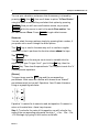
Press Y= . This bring up a flashing cursor to the right of Y1= in your
display window.
Step 2: At the flashing cursor we begin typing in our function
carefully:
3 X,T,θ,n ^ 3 − 13 X,T, θ,n ^ 2 − 10 X,T, θ,n + 50
Although spaces have been used between the above numbers for
clarity, don’t type spaces on the graphing calculator. Here’s how your
display should look:
Y1 =3X^3–13X^2–10
X+50
Y2=
Y3=
Y4=
Our font is a little different from that of the graphing calculator but
hopefully you get the picture. Notice the use of the ^ key. It
indicates to the graphing calculator that the operation is a
power/exponent.
Step 3: Now we graph the polynomial function defined in Step 2 by
pressing GRAPH .
You should see a display
similar to the one shown
here:
Step 4: We identify the approximate value(s) of the zero(s) by
inspection of the graph. Sometimes we need to adjust the viewing
window a little so that we can see where/if the x- intercepts or zeros
occur, but in this case all three are visible. A cubic polynomial can
have, at most, three Real zeros, so we need not worry that some are
not visible.
Module 1
10
Section 1, Lesson 1
Principles of Mathematics 12
a) The least zero is in the interval {−3,−1} (i.e., between −3 and −1). A
guess might be −2.0.
b) The middle zero is in the interval {2,3} (between 2 and 3). A guess
might be 2.5.
c) The greatest zero is in the interval {4,5} (between 4 and 5). A
guess might be 4.5.
Step 5: Now we will solve for the actual zeros, one by one. The
calculator needs a few details. The TI-83 will expect to receive them
in this very specific order:
Function, Variable, Guess, {Lower bound, Upper bound}
At this point, different calculators use different key sequences to
solve equations. The remaining steps 6–10 are for the TI-83. If you
are using a different calculator, look in the index of its user manual
under “Solving equations”.
Be sure to:
• use the X,T,θ,n key for X.
• use the minus key within the equation itself.
• use the negation (-) key for the guess and the bounds.
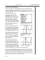
Want to know the math behind the button? Calculators and computers
solve functions with some form of Isaac Newton’s method. On a graph,
Newton’s method finds solutions or zeros (x-axis crossing points) like this:
using your initial “guess” and the slope of the graph at the point of your
guess, it calculates where that slope (a straight line, of course) crosses the
x-axis. Then it takes the crossing point as a second guess—it goes to the
graph point directly ‘above’ or ‘below’ where the first slope crossed the xaxis. It calculates the new slope of the equation at that point, goes to where
that new slope crosses the x-axis, and repeats the process.
If a guess is close to a zero or solution—to a point where the graph crosses
the x-axis—you can see that the graph’s slope from that point will be
almost parallel to the graph itself; the slope’s crossing point on the x-axis
will be close to the crossing point of the graph. Only a few repeats will be
needed, before it homes in on the actual crossing point. In reality, graphing
calculators perform so many repeats of Newton’s method in the time it
takes to press one button that your first guess need not be all that close to a
true solution. Just make sure that your first guess is clearly closer to one
solution (or crossing point) than it is to any other solutions. Better yet, set
the Lower and Upper Bound so that they contain only one crossing point. If
your guess is sort of midway between two crossing points, you can’t control
which one Newton’s method will find!
Module 1
Principles of Mathematics 12
Section 1, Lesson 1
11
Do type in the commas, and do not use spaces.
TI-83
Step 6
Press MATH , scroll down to option 0:Solver…. Select it with
ENTER .
You should now see:
EQUATION SOLVER
Eqn:0=
If you do not see EQUATION SOLVER, scroll up.
If you see an equation already written in, use the cursor-up (uparrow) key to place the cursor on the equation. Then use the
CLEAR key to remove it.
Step 7
Type the following equation exactly.
3X^3 – 13X^2 – 10X + 50
Then press ENTER
Next to the X= on the next line, type your first guess: –2.0
(remember to use the negation key, not minus).
On the bound= line, type your lower and upper bound (for the
first guess) between braces, like this: {–3, –1}
Finally, place your cursor on the X= line and press ALPHA
SOLVE . (ALPHA is the green key near 2nd, and SOLVE is on
the ENTER key)
Step 8
Your answer appears: X=–1.920589771 which we round to
–1.921.
If your answer is different, look carefully at your equation for
mistakes. Use the cursor keys to locate and correct them.
Step 9
Go back to Step 7. Change your bound= line to {2,3} and your
X= guess to 2.5.
Then press ALPHA SOLVE .
Ensure you get the answer 2.07815274 which rounds to 2.078.
If you got a BAD GUESS message, it means your guess is
outside your bounds.
Step 10
Go back to Step 7 and use your third guess of 4.5 and bounds of
4 and 5.
Then press ALPHA SOLVE .
Ensure you get the answer 4.175770562 which rounds to 4.176.
So the three solutions for the equation 3x3 – 13x2 – 10x = –50 from
least to greatest are: 1.921, 2.078, and 4.176.
Module 1
12
Section 1, Lesson 1
Principles of Mathematics 12
Adjusting the Viewing Window
Finally, we adjust the “viewing window” on the calculator so that
more of the graph is visible. Recall that the graph you saw on your
calculator (see page 9) went off the top and bottom of the screen—you
could not see it all.
To fix that, you adjust the
Viewing Window. Press the
WINDOW button at the top of
the keyboard. You see the list of
values at the right. From the
top, these values tell you that
the X-axis in your window ranges
from –10 to +10, with a tic-mark
for every number. The same is
true for the Y-axis.
Co-ordinate values for the Standard
Viewing Window on the TI-83.
For your graph to “look right,”
adjust the scale so that there are
fewer values displayed along the
X-axis (from –5 to +5, say) and
more displayed along the Y-axis.
As a first guess, use your cursor
to set Xmin = –5 and Xmax = 5.
Likewise, set Ymin = –30 and
Ymax = 30. Then press GRAPH
again. Now the graph looks like
the one at right.
The graph with the WINDOW
parameters at Ymin = –30 and
Ymax = 30
This is better, but we're still
missing the upper loop of the
graph. Our final adjustment is to
change Ymax to +60. That yields
the more appropriate display to
the lower right. We could change
X [ –5, 5 ] Y [ –30, 60 ]
the Xmin value from –5 to –3 for
a more balanced look, but what we have is good enough.
When you answer graphing-calculator questions on the Provincial
Exam, you will hand-sketch the graph in your calculator's viewing
window, then write in the Xmin and Xmax, and Ymin and Ymax
values, which you set for your window. The example at right shows
the correct way to write your window settings.
Module 1
Principles of Mathematics 12
Section 1, Lesson 1
13
Guided Practice
Solve each of the equations below using your graphing calculator and
showing the following detail:
Sketch the display as you see it.
For each of the possible solutions:
a) state your “guess”.
b) indicate the upper and lower bounds for x using interval notation.
For example {5,7} would indicate that x falls between 5 and 7.
c) state the actual solutions, correct to three decimal places.
Your graph sketch goes here.
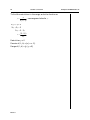
1. x3 – x2 – 12x = –3
X[
,
] Y[
,
]
X[
,
] Y[
,
]
2. –x3 + 2x2 – x + 1 = 0
Module 1
14
Section 1, Lesson 1
Principles of Mathematics 12
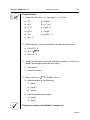
3. x3 + 6x2 + 3x – 5 = 0
X[
,
] Y[
,
]
X[
,
] Y[
,
]
X[
,
] Y[
,
]
4. x3 – 3x2 = 9x – 9
5. 0.25x3 – 0.5x2 – 6x – 2 = 0
Check your answers in the Module 1 Answer Key.
Module 1
Principles of Mathematics 12
Section 1, Lesson 2
15
Lesson 2
Functions and Interval Notation
Outcomes
Upon completing this lesson, you will be able to:
• identify the domain and range of various functions using set
notation and interval notation
• find the x- and y-intercepts of any function
• perform operations on functions
Overview
The concepts of domain and range are necessary to describe
functions. Interval notation is a most convenient way to describe
domain and range. We will also review combinations of functions and
composition of functions.
Definitions
A function is a relation where each x-value has only one
y-value
For any function, y = f(x), the domain is the set of possible
x-values, and the range is the set of possible y-values.
We can evaluate a function at a particular point by substituting
either numbers or algebraic constants into the f(x) expression and
simplifying the result.
Example 1
If f(x) = x3 – 2x, find f(0), f(–2), and f(a)
f(0) = 03 – 2(0) = 0
f(–2) = (–2)3 – 2(–2) = –8 + 4 = –4
f(a) = a3 – 2a
Module 1
16
Section 1, Lesson 2
Principles of Mathematics 12
Example 2
State the domain and range of the function p(x) = –2(x – 1)2 + 3
y
There is no restriction on the
values that x can take.
(1,3)
Domain = ℜ
x
The parabola has a maximum
value at (1,3)
Range = {y|y < 3, y ∈ ℜ}
Turn to Appendix 1 for some
background information on how
to read set notation.
Informal Rules for Finding a Function's Domain and Range
There is no “sure-fire formula” to determine the extent of a function
along the X-axis (its domain) or the Y-axis (its range). The domain
and range are often obvious if you just look at the graph; here are
some guidelines for finding the domain and range of a function by
looking at the equation, not the graph.
1. Linear functions, f(x) = mx + b, always have infinite domain and
range, in both directions (i.e., out to −∞ and also to +∞). The only
exception is when m = 0; then y = b and the domain remains
infinite but the range is simply b.
2. Parabolic functions, f(x) = a(x−h)2 + b, have infinite domain but a
limited range—the range goes to infinity in one direction on the
Y-axis, but not in the other direction. (This rule applies to any
even-powered function: x2, x4, x6 and so on.) If the exact range
boundary is not obvious from the equation, your graphing
calculator can identify it for you; this is taught in Lesson 4.
3. In square-root functions (with x somewhere under the root sign),
both the domain and range are infinite in one direction but not in
the other.
4. In any function where x appears in the denominator of a fraction,
watch out for specific values of x where the denominator becomes
zero. At those points the equation has no meaning (and the graph
shoots off to infinity along an asymptote). That x-value must be
excluded from the domain, and the corresponding f(x), or y value
(if there is one), must also be excluded from the range.
Module 1
Principles of Mathematics 12
Section 1, Lesson 2
17
You may find these guidelines helpful as you begin Math 12 and
work through the course. Most students find that domains and
ranges become obvious enough that they don't need these guidelines
for very long.
Example 3—Interval Notation
One way of reading the set {y|y ≤ 3, y ∈ ℜ} is “All the real numbers
between –∞ and 3.” On a number line, it would look like this:
•
0
3
We can write this interval from –∞ up to and including 3 as (–∞, 3].
The “(” means that the set doesn’t include –∞ (because infinity is
unreachable) and the “]” means that the point 3 is included in the
set.
So we see that another way of writing Range = {y|y ≤ 3, y ∈ ℜ} is
Range = (–∞, 3].
In this way we can rewrite ℜ as (–∞,∞).
{x | –4 < x ≤ 3} as (–4,3]
{x | 10 ≤ x ≤ l2} as [10,12]
{x | x ≥ –2} as [–2,∞]
An interval where the end points are both included is called a closed
interval and shown as [ ].
An interval where both end points are not included is called an open
interval and shown as ( ).
An interval where only one end point is included is called a halfopen interval and shown as either [ ) or ( ].
We can form the union of two intervals in the same way that we form
the union of two sets. Remember that ∪ is the symbol for union.
{x | x < –5, x ∈ ℜ}∪ {x | 0 < x < 4, x ∈ ℜ} can be written as
(–∞,–5)∪(0,4).
Most rational functions have restrictions because the denominator of
a function cannot be zero. The domain and range both have
restrictions. Interval notation is a convenient way to express a
restricted range or domain.
Module 1
18
Section 1, Lesson 2
Principles of Mathematics 12
Example 4
1
has asymptotes at x = ±2, and y
( x − 4)
= 0. It has a y-intercept at y = –1/4, but no x-intercepts.
The rational function f ( x ) =
2
Domain = {x | x ≠ –2, 2}. In interval notation this would be
(–∞,–2)∪(–2,2)∪(2,∞), which is very awkward.
Range = {y | y ≤ –1/4 or y > 0}. In interval notation, this would be
(–∞,–1/4)∪(0,∞).
y
x
x = –2
x=2
Note: Remember, an asymptote is a line that a curve approaches to infinity.
Combination of Functions
Two functions can be combined arithmetically by +, –, × or ÷. The
normal rules about addition, subtraction, etc. apply.
1
and g( x ) = 3 x − 2 , then we can
For example, if f ( x ) =
2x −1
create new combined functions by simple arithmetic like this:
f ( x ) + g ( x ) = ( f + g )( x ) =
1
+ 3x −2
2x −1
Note: There are two ways to show the addition of functions:
f(x) + g(x) or (f+g)(x).
Similarly, ( f − g )( x) =
1
− 3 x −2
2x −1
1
3x − 2
× 3x −2 =
2x −1
2x −1
1
1
( f ÷ g )( x ) =
÷ 3x −2 =
2x −1
(2 x − 1) 3 x − 2
( f × g )( x ) =
Module 1
Principles of Mathematics 12
Section 1, Lesson 2
19
Rule: When functions are combined arithmetically like that, the
domain of the result is the intersection of domains from the two
functions—it’s the set of all points that belong in both the original
domains. The same is true of the combined range—it’s the
intersection of the two separate ranges.
That intersection-of-domains rule applies for all four arithmetic
operations, between any two functions. But the division operation (f÷g)
has an additional rule: the combined domain and range cannot include
any value that makes the new denominator go to zero.
Note: Whenever this course uses a plain square root sign, it refers only
to the positive square root. This definition is common in
most modern mathematics.
Examples: If you solve x = 4 , then the answer is x = 2 but not
x = –2. If it wants the negative root, this course will ask you to
solve x = − 4 . If this course asks you for both roots, it will ask you to
solve x = ± 4 .
Example 5
Using the above two functions f and g, find the domain and range of
f+g, f–g, f×g, and f÷g.
Solution
By inspection, domain of f = {x|x ≠
f = {y | y ≠ 0}. x =
1
2
1
2
} and the range of
and y = 0 are not allowed because f cannot
have a zero in the denominator.
2
Similarly, domain of g = [ 3 ,∞)
The square root of a negative
number is not real so g cannot
be less than 32 . But the value
Range of g = [0,∞)
2
3 is in the domain of g.
Now for the intersections. Remember that ∩ is the symbol for
intersection:
Domain of (f+g) = domain of (f–g) = domain of (f×g) =
{x | x ≠ 12 } ∩ [ 32 ,∞) = [ 32 ,∞).
Module 1
20
Section 1, Lesson 2
Principles of Mathematics 12
Range of (f+g) = range of (f–g) = range of (f×g) = [y | y ≠ 0} ∪ [0,∞) =
[0,∞).
2
2
The domain of (f÷g) = ( 3 ,∞) instead of [ 3 ,∞). That’s because g(x) is in
2
2
the denominator and g( 3 ) = 0. So 3 must be deleted from the
combined domain.
The range of (f÷g) is (0,∞), just as it is for f+g, f–g, and (f×g). The
value 0 was excluded from the range of f already, so it’s not going to
appear in the range of the combined function.
Sometimes, when you write the range or domain of a combined
function, it may be simpler to leave the intersection symbol ∩ in your
answer.
Finding Intercepts
For more complex functions, we often need to know the x- and yintercepts in order to find the domain and range.
Rule: To find the y-intercept, set x = 0. To find the x-intercept, set y = 0.
Example 6
Find the x- and y-intercepts for the function, f(x) = x2(x + 1)(x – 2)
Solution
y-intercept: Set x = 0
f(0) = 02(0 + 1)(0 – 2) = 0
x-intercepts: Set y = 0
Solve: x2(x + 1)(x – 2) = 0
x2 = 0, or x + 1 = 0, or x – 2 = 0
∴x = 0, –1, or 2
Composition of Functions
A composition of two functions is when they are arranged so that one
is a function of the other.
Composition is not the same as “combination” using arithmetic
operations between functions!
Module 1
Principles of Mathematics 12
Section 1, Lesson 2
21
The composition is written as (f°g)(x) = f(g(x)) or as (g°f)(x) = g(f(x)),
either with a small hollow circle for the operation, or with one
function nested inside the other. In this course, f(g(x)) is the usual
notation but we’ll start by using both forms.
Example 7
If f(x) = x – 3 and g(x) = 2x + 1, find (f°g)(x) and (g°f)(x).
(f°g)(x) = f(g(x))
= f(2x + 1)
= (2x + 1) – 3
= 2x – 2
(g°f)(x) = g(f(x))
= g(x – 3)
= 2(x – 3) + 1
= 2x – 5
Substitute formula for g(x)
Apply formula for f(x)
Simplify
Substitute formula for f(x)
Apply formula for g(x)
Simplify
Notes to remember:
1. As Example 7 suggests, (g°f)(x) ≠ (f°g)(x) except in special cases.
2. For (f°g)(x) = f(g(x)), the range of g becomes the domain of f.
Example 8
If f(x) =
3
x
and h(x) = 2(x + 1), write an equation for (f°h)(x).
Specify the domain and range.
Solution
(f°h)(x) = f(h(x))
=
3
2 (x + 1)
To find the restrictions on the domain, remember that the
denominator cannot be zero.
2 (x + 1 ) ≠ 0
x ≠ −1
Module 1
22
Section 1, Lesson 2
To find the restrictions in the range, write the function as
y=
3
, rearrange and solve for y.
2 (x + 1)
2 y (x + 1) = 3
2 xy + 2 y = 3
2 xy = 3 – 2 y
x=
(3 − 2 y)
2y
Restriction: y ≠ 0
Domain of (f ° h) = {x | x ≠ –1}
Range of (f ° h) = {y | y ≠ 0}
Module 1
Principles of Mathematics 12
Principles of Mathematics 12
Section 1, Lesson 2
23
Guided Practice
1. Given that f(x) = 4x2 – x + 3 and g(x) = 1 – 2x, find:
a) f(0)
g) (f+g)(x)
b) g(0)
h) (g – f)(x)
c) f(–2)
i) (f×g)(–2)
d) g(1/4)
j) (f÷g)(0)
e) f(a)
k) (g÷f)(b – 1)
f)
g(b – 1)
2. Determine the x- and y-intercepts for the following functions:
a) f(x) = 2x2 – 8
b) g( x ) = 2x + 5
c) k(x) = 5 – x
3. Using the information from your answers to question 2, write the
domain and range for each function using:
i)
set notation
ii) interval notation
4. Given that p( x ) = x − 4 and q(x) = 3x + l:
a) determine each of the following:
i) p(q(x))
ii) p(q(3))
iii) q(p(a))
b) find the domain and range of:
i) p(q(x))
ii) q(p(x))
Check your answers in the Module 1 Answer Key.
Module 1
24
Section 1, Lesson 3
Principles of Mathematics 12
Lesson 3
Inverse Functions
Outcomes
Upon completing this lesson, you will be able to:
• verify that two functions are inverses of each other
• identify one-to-one functions
• find inverse functions
Overview
Many of the important new functions you will learn about in
Principles of Mathematics 12 are the inverses of other functions.
The concept of an inverse is essential to solving mathematics
problems.
Definition
Inverse Function: Let f and g be two functions such that
f(g(x)) = x for every x in the domain of g and g(f(x)) = x for every x
in the domain of f.
Then the function g is the inverse of the function f, denoted by f–1.
Thus f(f–1(x)) = x and f–1(f(x)) = x. The domain of f must be equal
to the range of f–1 and vice versa.
The graphs of f and f–1 are related to each other in this way. If
the point (a, b) lies on the graph f, then the point (b, a) lies
on the graph of f–1 and vice versa. This means that the graph
of f is a reflection of the graph of f–1 in the line y = x.
Module 1
Principles of Mathematics 12
Section 1, Lesson 3
25
From Principles of Mathematics 11, you may remember that:
1. The inverse of a function is its reflection in the line y = x. Each
point in the inverse function is the same distance away from the
line, but on opposite sides of the line. Every point (a,b) is
transformed to (b,a).
y
f 1(x )
f(x )
x
2. For an inverse function to exist, the original function must be
one-to-one. Every x-value must have only one y-value and vice
versa. Thus, the graph of the function must pass both the vertical
and horizontal line tests. Passing the vertical line test means that
the original function is truly a function; passing the horizontal
line test means that the inverse will also be a function. (Failing
the vertical line test means that we have a relation, but not a
function, like the circle relation in the illustration on the next
page.)
Module 1
26
Section 1, Lesson 3
y
Principles of Mathematics 12
y
x
x
One-to-one function.
Has an inverse function.
Not one-to-one.
Horizontal line cuts
the graph at two points.
Inverse is not a function.
y
x
Not a function. Vertical line cuts
the graph at two points. Inverse
will not be a function either
because a horizontal line does
the same.
Sometimes in Principles of Mathematics 12, we will get around
this restriction by considering only a portion of the original
function say, a piece of the graph which passes both line tests,
even if the whole graph passes only the vertical test.
3. In the inverse function, range and domain get reversed:
The domain of f(x) becomes the range of f–1(x).
The range of f(x) becomes the domain of f–1(x).
4. To find the inverse of a function y = f(x), replace x and y with each
other and solve for y.
Module 1
Principles of Mathematics 12
Section 1, Lesson 3
27
Example 1
Find the inverse of f(x) = 2x – 5
x = 2y − 5
replace x and y with each other
2y = x + 5
solve for y
x +5
y=
2
x +5
f −1 (x ) =
2
Check that your answer is correct by showing that f(f –1(x)) = x and
f –1(f(x)) = x
2( x + 5)
−5 = x
2
2x − 5 + 5 2x
f −1 ( f ( x )) =
=
=x
2
2
x +5
∴ f −1 ( x ) =
is indeed the inverse of f (x) = 2 x − 5
2
f ( f −1 ( x )) =
Example 2
1
. The domain of f(x)
a) Find the inverse of the function f ( x ) =
( x + 2)
is [0,∞).
b) State the domain and range of f(x) and f –l(x)
Solution
1
x+2
1
x=
y +2
a) y =
replace f ( x) by y
swap x and y
x ( y + 2) = 1
y=
solve for y
1
−2
x
∴ f −1 ( x ) =
1
−2
x
Module 1
28
Section 1, Lesson 3
Principles of Mathematics 12
Check:
(
) (
f f −1 (x ) =
=
1
x
1
)
−2 +2
1
1
x
=x
f −1 (f (x )) =
1
1
x +2
−2
= x +2−2
=x
b) domain of f = [0,∞) (given)
1
range of f = (0, 2 ] (the maximum value of f is
1
2
when x = 0)
1
domain of f –1 = range of f = (0, 2 ]
range of f –1 = domain of f = [0,∞)
Example 3
Given f ( x ) =
Step 1
Step 2
2x
, find f −1( x)
x +1
y=
2x
x +1
Replace f(x) with y to make manipulation
easier
x=
2y
y +1
Switch x and y variables
Step 3
x( y + 1) = 2 y
To isolate y, you need to eliminate fractions
by multiplying both sides by (y + 1)
Step 4
xy + x = 2 y
Expand bracket
Step 5
xy 2 y = x
Collect terms with “y” variable on one side
Step 6
y( x 2) = 2
Factor left hand side
Step 7
Module 1
y=
x
x 2
Divide both sides by (x – 2)
Principles of Mathematics 12
Section 1, Lesson 3
29
Guided Practice
1. For each of the following functions, f:
i)
ii)
iii)
find its inverse, f –1
check your answer by showing that f(f –1(x)) = x and
f –1(f(x)) = x
find the domain and range of f and f–1
a) f ( x ) =
x
3
b) f ( x ) = x 2 − 2
c) f ( x ) = 3 x − 2
d) f ( x ) =
1
, x ≥0
x −3
2. Find f –1(x) given
f ( x) =
x +1
3x
Check your answers in the Module 1 Answer Key.
Module 1
30
Notes
Module 1
Section 1, Lesson 3
Principles of Mathematics 12
Principles of Mathematics 12
Section 1, Lesson 4
31
Lesson 4
Polynomial Functions and Their Graphs
Outcomes
Upon completing this lesson, you will be able to:
• identify a polynomial function
• relate its factors to its zeroes
• graph a polynomial function
Overview
A polynomial function is an expression that can be written in
he form an x n + an −1x n−1 + … a 2x 2 + a 1x + a 0 where n is a nonnegative integer. In the above polynomial, each of the anx parts is
called a term. Terms are always added together (or subtracted) in
polynomials—never multiplied. The ai values are called coefficients
of the terms.
Notes
1. The graph of a polynomial function is continuous. This means the
graph has no breaks—you could sketch the graph without lifting
your pencil from the paper.
2. The graph of a polynomial function has only smooth turns. The
graph of f has, at most, (n – 1) turning points. Turning points are
points at which the graph changes from increasing (as we move to
the right) to decreasing or vice versa.
y
4
Dl
l B
cr
ng
de
si
cr
s in
ea
ea
3
E
in
g
2
co n s ta n t
l
l 1
A
x
1
2
3
4
Module 1
32
Section 1, Lesson 4
Principles of Mathematics 12
The function shown above is decreasing in the interval from D to
E, it remains constant from E to A, and it is increasing in the
interval from A to B. (Incidentally, because of its sharp corners
and its flat section, it cannot be the graph of a polynomial
function.)
For the graphs that you investigated, the cubic equation will have
at most (3 – 1) turns, or two turns. For the graphs that you
investigated, the quartic equations will have at most
(4 – 1) turns, or 3 turns.
3. a) When the degree, n, of a polynomial is odd
(i.e., of degree 1, 3, 5, ...):
If the leading coefficient is positive
(> 0), then the graph falls to
the left and rises to the right.
y
x
Another way to express this is
the graph rises from the third
quadrant.
If the leading coefficient is negative
(< 0), then the graph rises to
the left and falls to the right.
y
x
Or it falls from the second
quadrant.
b) When the degree, n, of a polynomial is even
(i.e., of degree 2, 4, 6, ...):
If the leading coefficient is positive
(> 0), then the graph rises to
the left and right, or “opens
up”.
If the leading coefficient is negative
(< 0), then the graph falls to the
left and right, or “opens down”.
y
x
y
x
Module 1
Principles of Mathematics 12
Section 1, Lesson 4
33
4. The function, f, has at most n real roots. If you have a cubic
function, you can expect three roots at most.
When you have a quartic function, you can expect it to have at
most four roots, and so on.
y
3
f(x) = –x + 4x
cubic—at most
three roots
x
4
2
f(x) = x – 5x + 4
quartic—at most
four roots
y
x
5. In general, the graph of a cubic function is shaped like a
“sideways S” as shown.
3
2
Graphs of f(x) = ax + bx + cx + d:
a>0
a<0
Module 1
34
Section 1, Lesson 4
Principles of Mathematics 12
In general, the graph of a quartic equation has a “W shape” or an
“M shape.”
4
3
2
Graphs of f(x) = ax + bx + cx + dx + e:
a>0
a<0
2
6. If a polynomial f(x) has a squared factor such as (x – c) , then x = c
is a double root of f(x) = 0. In this case, the graph of
y = f(x) is tangent to the x-axis at x = c, as shown in Figures 1, 2,
and 3.
y
Figure 1
Cubic
2
y = (x – 1)(x – 3)
x
y
Figure 2
Quartic
2
y = (x – 1)(x – 3) (x – 4)
x
Module 1
Principles of Mathematics 12
Section 1, Lesson 4
y
x
35
Figure 3
Quintic (5th degree)
2
2
y = x (x – 1)(x – 3)
[which is a more efficient
way of writing
y = (x – 0)2 (x – 1)(x – 3)2]
3
If a polynomial P(x) has a cubed factor such as (x – c) , then x = c
is a triple root of P(x) = 0. In this case, the graph of
y = P(x) flattens out (or plateaus) around (c, 0) and crosses the xaxis at this point, as shown in Figures 4, 5, and 6.
Figure 4
Cubic
3
y = (x – 2)
y
x
y
Figure 5
Cubic
3
y = –(x – 2)
x
Module 1
36
Section 1, Lesson 4
y
Principles of Mathematics 12
Figure 6
Quartic
3
y = (x – 1) (x – 3)
x
7. Polynomial functions may have relative maxima, relative
minima, absolute maxima or absolute minima or a combination.
See the above Figure 6 for an example of absolute and relative
minima. The absolute minimum at (2.25, –1.75) and a relative
minimum at (1,0). Absolute and relative maxima would exist if
the graph opened down.
Example 1
Sketch the graph of the function, f(x) = x2(x + 1)(x – 2). Find the
maximum and minimum points.
Solution
Find the y-intercept. Set x = 0.
f(0) = 02(0 + 1)(0 – 2) = 0
Therefore (0,0) is the y-intercept for this function.
Find the x-intercepts. Set y = 0
x2(x + 1)(x – 2) = 0
x2 = 0 or x + 1 = 0 or x – 2 = 0
x = {–1,0, 2}
The term with the highest power is x4 (found by multiplying together
the x terms in the equation: x2 × x × x = x4), so the function is a
quartic, or fourth order, polynomial.
The coefficient of x4 is positive, so the graph “opens up.” x2 is a
double root, so the graph touches the x-axis at x = 0.
Module 1
Principles of Mathematics 12
Section 1, Lesson 4
37
The interval (–1,0) between the roots
is less than the interval (0,2), so the
graph goes down farther between 0
and 2. Note that we have a relative
minimum in the interval (–1,0), a
relative maximum at (0,0), and an
absolute minimum in the interval
(0,2). To determine range, we need
to find the value of the absolute
minimum. We can do this using the
“minimum” choice from the CALC
menu of a graphing calculator.
Press Y= . At the flashing cursor, carefully type
X,T,θ
x 2 ( X,T,θ + 1)( X,T,θ – 2)
Your display should look like this:
Y1 x 2 (x +1)(x - 2)
Y2
Y3
etc.
Press GRAPH to see your display.
Press WINDOW to obtain the WINDOW or WINDOW FORMAT
menu. Change the Ymin setting to –5 in order to better see the
minimum value.
To calculate the minimum value, press 2nd TRACE to get the
CALC ulate menu. Scroll down to 3:minimum or press 3. You will
notice the blinking cursor on the graph (if not, use left arrow key to
activate). Use the arrows to move the cursor to the left of the lowest
minimum value, and press ENTER . Use the right arrow to move
the cursor to the right of the lowest minimum value and press
ENTER again. Move the cursor back close to the minimum as your
guess.
Module 1
38
Section 1, Lesson 4
Principles of Mathematics 12
Press ENTER again.
The minimum occurs at (+1.443001, –2.833422).
Therefore range = [–2.833,∞), or {y|y ≥ –2.833]. We use a closed interval
because the graph reaches down to approximately –2.833.
Example 2
Inspect the following polynomial functions and determine their basic
shape and orientation.
Determine the domain and range of each.
a) f(x) = x3 – 4x
b) g(x) = –x6 + 4x2
c) k(x) = –x5 + 4x3 – 6
Hint: The absolute minimum or absolute maximum always defines
the range.
Solutions
a) f(x) is a third order (cubic) polynomial, with a positive leading
coefficient. The graph rises from Quadrant III in an S shape.
Furthermore, when factored, f(x) = x(x – 2)(x + 2), we can easily
find its zeroes.
Solving x (x – 2)(x + 2) = 0, we
get x = –2, 0, or 2. Because it
has 3 roots,
it has 3 – 1 = 2 turns.
domain = ℜ and range ℜ
b) g is a sixth order polynomial, with a negative leading coefficient,
so it opens down.
When factored, we see that g(x) = –x2(x2 + 2)(x2 – 2)
x2 is a repeated factor
x2 + 2 has no real factors
x 2 − 2 = 0 yields x 2 = 2, so x = ± 2
Module 1
Principles of Mathematics 12
Section 1, Lesson 4
39
The maximum number of
turns is 6 – 1 = 5, but because
of the x2 + 2 factor we only get
3 turns.
domain = ℜ
Using the graphing calculator
as in
Example 1, we get
range = (–∞, 3.0792014]
c) k is a fifth order polynomial, or quintic, which means it is an odd
polynomial. It has a negative leading coefficient, so it falls from
Quadrant II. It has at most 5 – 1= 4 turns.
domain = ℜ
range = ℜ
When we plot it using the
graphing calculator, we find it
has only one maximum and one
minimum, with a kink near the yaxis called a stationary point
(which you don’t have to
remember).
The local maximum is located
(1.54591952,
–0.0510976).
In Lesson 1 to solve an equation with the graphing calculator, we
used the “0:Solver” function from the MATH menu and
typed in the equation to be solved. That method works, but we
could miss a solution for a higher-order polynomial because there can
be several solutions close to each other.
Module 1
40
Section 1, Lesson 4
Principles of Mathematics 12
To find the zero (x-intercept) of a graphed equation, press 2nd
CALC
, then 2:zero. Just as you did for a minimum or maximum,
mark the left bound, right bound, and a first guess for each
crossing point on the x-axis. (Include only one crossing point between
your left and right bounds.) Then write down the displayed x-value
as the solution. Repeat for each crossing point on the x-axis.
In this case c) you'll find a zero at –2.146348, which you round to
–2.146. If you try the same thing for the relative maximum, near x =
1.5, which appears to touch the x-axis, you'll get an error message.
That’s because the graph does not quite reach the x-axis there; the yvalue reaches –0.051 but not 0.
You can solve equations using either MATH 0:Solver or CALC
2:zero. Because the 2:zero function works off a graph, it gives you a
better chance of noticing and reporting every solution.
Module 1
Principles of Mathematics 12
Section 1, Lesson 4
41
Guided Practice
1. Rewrite each polynomial in descending order. Determine:
i)
ii)
the degree of the polynomial
the maximum number of turns in the graph
a) f ( x ) = 8 x − x 4
b) g ( x ) = x 3 + 5 x 4 − 2 x 2
c) h( x ) = −3 x 5 − x 2 + x
2. State the left-right behavior of the graphs in question 1, as to
whether they open up, open down, rise from Quadrant III, or fall
from Quadrant II.
3. Match each polynomials function with the correct graph.
a) f (x ) = −3 x + 5
b) f (x ) = x 2 − 2x
c)
f (x ) = −2x 2 − 9 x − 9
d) f (x ) = 3 x 3 − 9 x + 1
1
2
e) f (x ) = − x 3 + x −
3
3
1
f) f (x ) = − x 4 + 2x 2
4
g) f ( x ) = 3 x 4 + 4 x 3
h) f ( x ) = x 5 − 5 x 3 + 4 x
Module 1
42
Section 1, Lesson 4
i)
ii)
iii)
Module 1
Principles of Mathematics 12
Principles of Mathematics 12
Section 1, Lesson 4
43
iv)
v)
vi)
Module 1
44
Section 1, Lesson 4
Principles of Mathematics 12
vii)
viii)
4. Find (i) the zeros of the following functions, (ii) the maximum
number of turns, (iii) the left-right behaviour, (iv) the domain and
range, and (v) sketch the graph of the function.
a) f (x ) = 4 x − x 3
b) g (x ) = ( x − 2)4
c) h (x ) = x 3 + x 2 − 6 x
Check your answers in the Module 1 Answer Key.
Module 1
Principles of Mathematics 12
Section 1, Review
45
Review
1. Solve the following equations using your graphing calculator.
a) x 3 + 2x 2 − 4x = 7
b) 2 x 4 + 3 x 2 = 4
c) x 5 − 4 x 3 = x 2 − 3 x
d) 0.4 x 3 − 0.78 x 2 + 2.4 x + 7 = 0
2. If f (x ) = 3 x 2 + 3 x − 1 and g( x ) = 2 x + 1, find:
a) f (2)
b) g( −1)
c) ( f + g )(4)
d) ( f ÷ g )(4)
e) f ( a + 4)
f)
( g f )(1)
g) ( f g )( x )
h) f ( f −1 ( x ))
i)
( f × g )( t + 2)
j)
g −1 ( x )
3. i) Determine the x- and y-intercepts of these functions.
ii) Find the domain and range.
a) f ( x ) = 1 − 2 x
b) g ( x ) = 2( x + 2)2 − 4
c) h( x ) = ( x + 2)2 ( x − 4)( x − 2)
Module 1
46
Section 1, Review
Principles of Mathematics 12
4. Find the inverse of the following functions.
a) f ( x ) = 5 x − 2
b) g ( x ) = ( x + 1)2 − 3
c) h( x ) =
1
x −1
2
5. Sketch the graphs of the following functions. Label the intercepts
and give the domain and range of each.
a) f ( x ) = x 3 + x 2 − 2
b) g ( x ) = −2( x 2 − 9)( x + 2)(2 x −1)
Check your answers In the Module 1 Answer Key.
Now do the section assignment which follows this section. When it is
complete, send it in for marking.
Module 1
Principles of Mathematics 12
Section Assignment 1.1
47
Student's
Name _______________________________
Student
No. __________________________
Address _______________________________
School __________________________
_______________________________
Student's
_______________________________ FAX No. __________________________
Instructor's
Name _______________________________ Date Sent __________________________
PRINCIPLES OF MATHEMATICS 12
Section Assignment 1.1
Your instructor will fill in this box with your percentage mark and letter
grade on the section assignment:
Comments/Questions:
Version 06
Module 1
48
Section Assignment 1.1
Principles of Mathematics 12
General Instructions for Assignments
These instructions apply to all the section assignments but will not
be reprinted each time. Remember them for future sections.
(1)
Treat this assignment as a test, so do not refer to your module
or notes or other materials. A scientific calculator and
graphing calculator are permitted.
(2)
Where questions require computations or have several steps,
showing these can result in part marks for some exercises.
Steps must be neat and well-organized, however, or the
instructor will only consider the answer.
(3)
Always read the question carefully to ensure you answer what
is asked. Often unnecessary work is done because a question
has not been read correctly.
(4)
Always clearly underline your final answer so that it is not
confused with your work.
Module 1
Principles of Mathematics 12
Section Assignment 1.1
49
Section Assignment 1.1
Review of Mathematics 11
Total Value: 40 marks
(Mark values in margins)
1. If h( x ) =
3
, find:
2x + 1
(1)
a) h (2 )
(1)
b) h  − 1 
 2
Module 1
50
Section Assignment 1.1
Principles of Mathematics 12
c) h (a − 1)
(1)
d) h −1 (x )
(2)
Module 1
Principles of Mathematics 12
(4)
Section Assignment 1.1
2. For the the function g( x ) = 2x + 3
51
find:
a) the domain of g
b) the range of g
c) the y-intercept
d) the x-intercept
Module 1
52
Section Assignment 1.1
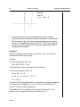
3. For the the function q(x) below, sketch the graph of q−1(x):
4. If f ( x ) = x 2 − 2 and g( x ) =
Principles of Mathematics 12
(1)
1
( x ≠ 0) , find:
3x
a) (f+g)(x)
(1)
b) (f × g)(–2)
(1)
Module 1
Principles of Mathematics 12
(1)
c) f(g(x))
(1)
d) g(f(–1))
(2)
e) f –l(x) where x ≤ 0
(5)
Section Assignment 1.1
53
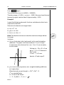
5. Without using your graphing calculator, sketch the graph of g(x)
= –2(x – 1)2(x + 3). Label the intercepts and give the domain and
range.
Module 1
54
6. Given f ( x ) =
Section Assignment 1.1
Principles of Mathematics 12
x −4
, find.f –l(x)
x +1
7. Find the maximum value of the function f(x) = –x4 – 3x2 + x + 7 and
use it to determine the range of f.
Module 1
(4)
(5)
Principles of Mathematics 12
Section Assignment 1.1
55
8. Solve using your graphing calculator:
(1)
a) 2x4 – 3x3 = x
(2)
b)
x 2 − 2x − 4
=x
2x 2 + x − 3
Module 1
56
Section Assignment 1.1
Principles of Mathematics 12
9. Given: f ( x ) = 2 + x
g( x ) = x − 7
h( x ) = 2 x 2 − 5
Determine:
a ) g(h( x ))
(1)
b) f (h(3))
(1)
c ) h( g( f ( −1)))
(2)
Send in this work as soon as you complete this section.
Module 1
Total: 37 marks