Download Chapter 1

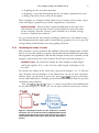
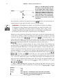
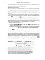
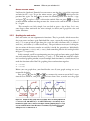
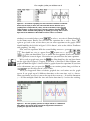
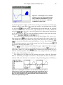
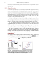
SAMPLE CHAPTER
MANNING
Using the TI-83 Plus/TI-84 Plus
by Christopher R. Mitchell
Chapter 1
Copyright 2013 Manning Publications
brief contents
PART 1
PART 2
PART 3
PART 4
BASICS AND ALGEBRA ON THE TI-83 PLUS/TI-84 PLUS.....1
1
■
2
■
3
■
4
■
What can your calculator do? 3
Get started with your calculator 25
Basic graphing 57
Variables, matrices, and lists 83
PRECALCULUS AND CALCULUS ...................................111
5
■
6
■
7
■
Expanding your graphing skills 113
Precalculus and your calculator 141
Calculus on the TI-83 Plus/TI-84 Plus
158
STATISTICS, PROBABILITY, AND FINANCE ....................171
8
■
9
■
10
■
Calculating and plotting statistics 173
Working with probability and distributions
Financial tools 223
202
GOING FURTHER WITH THE TI-83 PLUS/TI-84 PLUS ...235
11
■
12
■
13
■
Turbocharging math with programming 237
The TI-84 Plus C Silver Edition 260
Now what? 282
iii
What can your
calculator do?
This chapter covers
■
Hands-on examples of your calculator’s
features
■
Using your calculator faster and better
■
MathPrint and why you might need it
A graphing calculator is one of the most powerful tools you can use in school or at
work. From the name, you can guess that it’s great at math, from the simplest arithmetic like 2 + 2, to calculating statistics and multiplying matrices. It’s also a pro at
graphing and helping you understand its graphs. You can use your graphing calculator for algebra, trigonometry, precalculus, and calculus; you can even use it to
write programs and games. If you’re a student or teacher, a graphing calculator can
be used in every math subject from middle school to college, as well as in science
and computer classes. Many graphing calculators are available from Texas Instruments, HP, and Casio; this book focuses on the TI-83 Plus, TI-84 Plus, TI-83 Plus Silver Edition, TI-84 Plus Silver Edition, and TI-84 Plus C Silver Edition, but it can help
you use all the calculators shown in figure 1.1.
Your calculator can also be an intimidating device, with so many functions and
buttons. It certainly looks harder to use than other familiar gadgets, like a cell
phone or a handheld game console. Instead of a mouse or touchscreen, you use
3
4
CHAPTER 1
What can your calculator do?
Figure 1.1 Calculators covered in this book (from left): TI-82, TI-83, TI-83 Plus, TI-83 Plus Silver
Edition, TI-84 Plus, TI-84 Plus Silver Edition, and TI-84 Plus C Silver Edition. The focus is on the TI-83
Plus and TI-84 Plus models, although most of the skills and examples also apply to the TI-82, TI-83, and
TI-82 Stats.fr.
the keyboard to navigate through its features. Fear not—complicated though it might
look, you can easily become a calculator expert, and this book will hold your hand
every step of the way. Whether you use this guide as a quick reference to do something
specific or do a thorough read to learn how to use your calculator well, you’ll find lessons taught with simple steps and fun examples. This chapter will immediately show
you some calculator skills and demonstrate the variety of tasks a graphing calculator
can help you do.
We’ll start with five examples of what you can use your calculator for: algebra, geometry, graphing, calculus, and statistics. You can go through them one by one, trying them
on your own calculator, skip around, or just peruse them. You’ll find a section describing more about this book and how it can help you use your calculator and then a discussion of which calculators this book will teach. You’ll learn the difference between
MathPrint and non-MathPrint calculators (this book covers both) and end with a look
forward at the basic calculator skills you’ll discover in chapter 2. Let’s get started with
five fun examples and see how easy and powerful a graphing calculator can be.
1.1
Five examples of what your calculator can do
Your calculator can solve countless different kinds of math and science problems and
help you double-check your work while doing homework or during tests (even the
SAT!). To help you jump right into using your calculator, let’s start with five complete
examples, picked from exactly the sort of problems you might encounter in class. If
you’d prefer to start learning specific math skills immediately, you might want to skip
this section, skim the rest of chapter 1, and then begin with the arithmetic and algebra
skills in chapter 2. If you want to see some examples of what your calculator can do,
here’s what this section will cover:
1
2
Calculating the volume of a cube and then cutting off the top of the cube and
finding the new volume
Finding solutions to the Quadratic Formula, a method for solving ax2 + bx + c = 0
Five examples of what your calculator can do
3
4
5
5
Graphing the sine and cosine functions
Graphing a curve and then figuring out the area under a portion of the curve
Fitting a line of best fit to a series of data points
These examples are arranged in order from easiest to hardest and are taken, respectively, from algebra, geometry, precalculus, trigonometry, and statistics.
BEFORE YOU BEGIN All five of these examples should work well on your calculator without any special setup. If you’re getting different answers for some
of the examples, consider resetting your calculator to its default settings.
Section 2.1 explains how to do that.
Let’s get started with the first example, finding the volume of a cube. Besides being a
nifty demonstration that might come in handy during a geometry class, it’s a great way
to begin doing useful arithmetic on your graphing calculator.
1.1.1
Calculating the volume of a cube
Your calculator is a pro at arithmetic like addition, subtraction, multiplication, and division. It can also raise numbers to powers and perform lots of mathematical operations
like logarithms and trigonometry. For our first example of what your calculator can do,
imagine a cube of which every side is 9 inches, like the one on the left in figure 1.2.
VOLUME OF A BOX To calculate the volume of a box, multiply its width, length,
and height together. If it’s a cube, then the width, length, and height are all
the same.
To calculate the volume of the 9-inch cube, you need to multiply 9 × 9 × 9. Turn on
your calculator, and you should be at the homescreen, the area of your calculator’s
software where you do math. If you’re not, press
to quit to the homescreen, which should have a blinking cursor and either be blank or show the previous
calculations you performed.
Next, type
to get 9*9*9 on the screen. Your screen should match
the left side in figure 1.3. There’s no = key on your calculator; instead, you calculate
Figure 1.2 Measuring the volume of a cube. On the left, a cube with
9-inch sides. You can calculate its volume by multiplying width × length
× height. On the right, the top 3 inches of the cube are cut off, and you
want to find the volume of the new box that is 6 inches high instead of
9 inches.
6
CHAPTER 1
What can your calculator do?
Figure 1.3 Two different ways to calculate
the volume of a cube with 9-inch edges. On
the left, multiply width × length × height to
get the volume, 729. You can also cube 9 by
raising it to the third power, which means
multiplying the number by itself three times
(right). Depending on what calculator type
and version you have, your results will look
like either the top or bottom; section 1.3 will
explain more.
the result of the arithmetic you typed by pressing
. You’ll see the result of the calculation printed at the right side of the screen: 729 cubic inches.
Throughout this book, I use TI-83 Plus/TI-84 Plus screenshots
to demonstrate most problems, interspersed with occasional TI-84 Plus C Silver Edition screenshots. No matter which calculator you’re using, all the
examples and skills in this book will work on any TI-83 Plus or TI-84 Plus–family calculator, even if what you see on the screen is a bit different.
SCREENSHOTS
Another way you can find the volume of a 9-inch cube is to take the length of one side,
9, and cube it. Cubing a number is raising it to the third power, written 93. On your
calculator, you type this as
and then press
. As you might expect, and
as the right side in figure 1.3 confirms, the result is still 729. Note that depending on
whether you have a MathPrint operating system on your calculator, the key sequence
might display different (but equivalent) math on your screen.
As a final exercise, imagine slicing the top 3 inches off the box. Perhaps you
needed to open it, or perhaps the cube was actually a 6-inch-tall box with a 3-inch lid
that you just took off. Either way, as the right side in figure 1.2 shows, you now have a
9-inch by 9-inch by 6-inch box, and you want to calculate the new volume. This time,
you must multiply 9 × 9 × 6, which is very similar to your previous experience multiplying 9 × 9 × 9. Figure 1.4 shows what the equation will look like when you type
; as before, the
key acts like an = key to make the volume of the
shorter box appear: 486. Because 9 × 9 is 9 squared, you could even be clever and type
9 × 9 × 6 as 92 × 6, which once again (as the right side in figure 1.4 demonstrates) produces the correct volume of the shorter box: 486. To type the squared symbol, you
could type
, but it’s faster to use the
key. Thus, to calculate 92 × 6, press
.
That’s a quick introduction to using your calculator for math. You type in the
expression to calculate with the number keys and operators like
,
,
, and
.
Figure 1.4 Calculating the volume of the 9-inch cube with the
top 3 inches sliced off. The last line shows the same calculation
using the
key instead of typing 9 × 9.
Five examples of what your calculator can do
7
You then ask your calculator to produce the result with
. Section 2.2 will teach
you more about basic arithmetic and your calculator.
A more complicated math example is solving the Quadratic Formula, which will
require using a few tools you haven’t seen yet.
1.1.2
Solving the Quadratic Formula
The Quadratic Formula is used to figure out values of the variable x that make a quadratic equation 0 = ax2 + bx + c true, once you pick three constant numbers a, b, and c.
If you’re not familiar with the notation, you can read it as “0 equals a times x squared,
plus b times x, plus c.” You square x, multiply the result by a, add that to b times x, and
add c. If you use a value of x that is a correct solution for the given a, b, and c, you’ll
get 0. For an x value that isn’t a solution, the result of that multiplication and division
will be a number other than 0. Even if you haven’t worked with this type of math
before, fear not! Follow along, and in later chapters (and math classes) you’ll learn
more about the Quadratic Formula.
MEET THE QUADRATIC FORMULA
You don’t need to guess values for x and plug them in. The Quadratic Formula is a
tool to find the 0, 1, or 2 values of x that satisfy (solve) 0 = ax2 + bx + c for a given set of
three constants a, b, and c. The Quadratic Formula is shown and demonstrated in
action in figure 1.5.
We’ll try solving for the roots of 0 = 2x2 + 8x + 2, where the roots are values of x that
make the right side of the equation equal to 0. In this case, a = 2, b = 8, and c = 2. The
top of figure 1.5 shows the Quadratic Formula, into which you’ll plug values for a, b,
and c. Your calculator can handle named variables, so you can store 2 into A, 8 into B,
and 2 into C (your calculator only has uppercase variables like A, B, X, and M). You’ve
seen the squared symbol (as in b 2) in the previous example, finding the volume of a
box. But there are two new symbols that you might be unfamiliar with.
The ± symbol means you can put either a plus sign or a minus sign at that position.
In other words, the Quadratic Formula is actually two different equations, one with a
plus and one with a minus. When you plug in a, b, and c, you get two solutions: one for
the equation with a plus and one for it with a minus. The other symbol that might be
x=
-b±
b2-4ac
2a
SOLUTION WITH DOUBLE ROOT
a=1, b=2, c=1
x=
-2±
x=-1
22-4*1*1
-2± 0
=
2
2*1
SOLUTION WITH REAL ROOTS
a=2, b=8, c=2
x=
-8±
82-4*2*2
-8± 48
=
4
2*2
x=-2± 3
Figure 1.5 The Quadratic Formula (top) solved for two sets of a, b, and c
constants. On the left, we set a = 1, b = 2, and c = 1, and get the double root
–1, –1. On the right, setting a = 2, b = 8, and c = 2 yields two difference roots,
–2 plus and minus the square root of 3.
8
CHAPTER 1
What can your calculator do?
new (but hopefully not!) is the radical or square root symbol, √. It indicates that you
should take the square root of everything inside.
STORING VALUES FOR A, B, AND C
Let’s set up your a, b, and c values into the A, B, and C variables on your calculator
first and then type the two different forms of the Quadratic Formula to find the solutions. We’ll try solving the case on the left in figure 1.5, where a = 1, b = 2, and c = 1.
From the figure, you can see that you should get two (identical) solutions, x = –1
and x = –1.
First, make sure you’re at the homescreen. You may have to press
to get
there or
to start with a blank line. The first thing you’ll do is assign (store) values
to the variables A, B, and C. The
key prints the → symbol, which takes whatever is
on its left side and stores it into whatever is on its right side. For example, 3→A stores
the number 3 into the A variable, whereas —4.5→X stores –4.5 (negative 4.5) into the X
variable. You can then use those variables in expressions; so if you calculated A+4 after
storing 3 into A, it would be like 3 + 4, and you would get 7 as the answer.
With that in mind, try these steps:
1
2
3
Type
. Don’t press
on the screen, as in figure 1.6.
Continue by typing
should now have 1→A:2→B:1→C on the screen.
Press
to store values to A, B, and C.
yet. You should see 1→A:
. You
Although the calculator will just print 1 at the right edge of the screen, as you can see
on the left side in figure 1.6, you executed three commands at once. You simultaneously put values in the three variables A, B, and C. On your calculator, you can separate
multiple commands or calculations with a colon (:); and when you press
, all the
commands or calculations will be performed from left to right. The calculator only
shows the result for the last operation, so if you typed 1+1:2+2:3+3 and pressed
,
the result would be 6. Why bother using colons instead of putting each store command on a different line? Because as you’ll learn in chapter 2, you can go back to lines
Figure 1.6 On the left, storing values a = 1, b = 2, and c = 1. These values can be
used in the Quadratic Formula, as shown in the center and right. The center
screenshot applies to TI-84 Plus, TI-84 Plus Silver Edition, and TI-84 Plus C Silver
Edition calculators running one of the MathPrint operating systems. The right
screenshot shows the same equation entered on a calculator without MathPrint. In
section 1.3, I’ll explain more about the MathPrint operating systems. Throughout
this book, I’ll show you how to do things both with and without MathPrint.
Five examples of what your calculator can do
9
you already entered and run them again; and if you set A, B, and C on the same line,
you can change them all by modifying one line instead of three.
Now that you have values in A, B, and C, it’s time to calculate the two solutions to
the Quadratic Formula. This is going to get a bit tricky, because depending on
whether you have a calculator with a MathPrint operating system (newer TI-84 Plus/
Silver Edition calculators) or a non-MathPrint operating system (TI-82, TI-83, TI-83
Plus/Silver Edition, and some TI-84 Plus/Silver Edition calculators), you’ll have to
enter a different series of commands.
SOLVING THE QUADRATIC FORMULA
Before we can continue, you need to figure out whether you have a MathPrint operating system and, moreover, whether the MathPrint mode is enabled. If you just stored
values to A, B, and C, you should still be at the homescreen. Press the
key, right
under the
key:
■
■
If the cursor is a dark square blinking inside a dotted square, next to and
slightly above the word Ans, you have MathPrint installed and enabled.
If the cursor is a dark rectangle blinking normally next to the text Ans^, with no
dotted line around the cursor, you either don’t have MathPrint installed or
have it disabled.
Without MathPrint: Type in the “plus” version of the Quadratic Formula (remember
the ± symbol?) with the following key sequence:
. Your screen should look like the right side in figure 1.6. If you made any mistakes, you can press
to clear the line and start over, or you can use the
and
arrow keys to move the cursor through the line, press
to delete extra symbols
or numbers, and press
to switch into Insert mode. When you’ve finished,
and your screen matches the right side in figure 1.6, press
. You should see the
answer, –1.
Notice that to type the negative symbol, you don’t press the subtract key. On your calculator, negative and subtract are two different keys. Notice also that your calculator does implicit
multiplication: 4AC is like 4*A*C.
NEGATION AND IMPLICIT MULTIPLICATION
With MathPrint: Type in the “plus” version of the Quadratic Formula with the following
key sequence:
. Your screen should look
like the right side in figure 1.6. The only difference from the non-MathPrint instructions is that you need to press
to get out of the square-root radical symbol, instead
of pressing the
key. As with the non-MathPrint instructions, you can use the
arrows,
, and
to move the cursor around, delete errors, and insert
missing numbers and symbols. When your entry looks like the center screenshot in
figure 1.6, press
, and you should get –1.
10
CHAPTER 1
What can your calculator do?
GETTING THE OTHER ANSWER
I told you the Quadratic Formula has two answers, one for the + case of the ± operator
and one for the – case. To get the minus answer, press
, which pastes the
previous line again. Use the
key to move the blinking cursor over the first + sign,
and press
to replace it with a subtraction symbol. You can press
to get the
second solution without needing to move the cursor to the end of the line: it should
be –1 again.
This example was fairly simple, but you had to press a lot of keys. Let’s save
your fingers some work with the next example, in which you’ll graph the sine and
cosine functions.
1.1.3
Graphing sine and cosine
Sine and cosine are two trigonometric functions. They’re periodic, which means that
they repeat over and over again. Both look like a wave, repeatedly curving between y = 1
and y = –1 as you go left to right along the x axis. On your calculator, sine() is abbreviated sin(), and cosine() is abbreviated cos(). The parentheses mean you’re taking the
sine or cosine of whatever number or variable is inside the parentheses. Individually,
the two equations y = sin(x) and y = cos(x) look something like the left and right sides
of figure 1.7, respectively.
In this example, you’ll be superimposing one sine graph and one cosine graph. Both
sine and cosine only alternate between y = 1 and y = –1. This looks tiny with the calculator’s standard graphing window, so you’ll multiply both functions by a coefficient of 5 to
make the functions taller. You’ll be graphing these two functions together:
Y1 = 5sin(X)
Y2 = 5cos(X)
Before you can graph these, you should make sure all your graph settings are set to
reasonable defaults.
First, press
, use the
and
keys to move the cursor to any of the Y= equations that are filled in, and press
to erase them. Next, to make sure the graph
Figure 1.7 Graphs of sin(x) (left) and cos(x) (right). These are both graphed from
x = –10 to x = 10, with limits of y = –3 at the bottom and y = 3 at the top. If you
know how to graph curves, and you can’t figure out why graphing sin(x) or cos(x)
on your calculator doesn’t look like these screenshots, try pressing
and
setting Ymin to –3 and Ymax to 3.
Five examples of what your calculator can do
11
Figure 1.8 Screenshots of graphing sine and cosine from a TI-83 Plus or TI-84 Plus.
On the left, the empty Y= menu, the same menu with the two functions you’re
graphing in this example filled in (center), and the result when you press
(right). Read the section to learn how to enter the equations and graph them, and
read the sidebar “Problems with graphing?” if anything goes wrong. Take a look at
figure 1.9 for the TI-84 Plus C Silver Edition versions of these screenshots.
window is set to useful values, press
to select 6:ZStandard (Zoom Standard)
in the Zoom menu. Finally, you can enter the equations for Y1 and Y2. Press
again to get back to the screen where you can enter equations to the graph, which
should look like the left side in figure 1.8. If it doesn’t, refer to the sidebar “Problems
with graphing?” for help.
Next, enter the equations. With the cursor flashing next to Y1=, press
. You should see 5sin(X) appear. Press
to move to Y2=, and press
. Now you should have 5cos(X) under the first equation. If you want, doublecheck against the center in figure 1.8 to make sure you and I have the same equations.
We’re ready to graph now: press the
key. You should see the two lines shown
on the right side in figure 1.8 appear. If you have a TI-84 Plus C Silver Edition, your
graph will look like figure 1.9 instead. You’ve graphed your first equations! If you want
to be adventurous, you can press the
key to examine points along each line or
to see the table view of x and y values.
What just happened? Your calculator graphed sine and cosine on the graph
screen. It can graph up to 10 different functions at the same time, so 2 is a breeze.
When you choose ZStandard, you set the top of the screen to y = 10 and the bottom to
y = –10. You multiplied both the sine and cosine functions by 5 so that the resulting
Figure 1.9 The same graphing operation as in figure 1.8 but on a TI-84 Plus C
Silver Edition. The left side shows entering two trigonometric functions for
graphing; the right side shows the result.
12
CHAPTER 1
What can your calculator do?
lines would alternate between y = –5 and y = 5 instead of –1 and 1. This makes them
much easier to see.
For our fourth example, we’ll move from precalculus to calculus to find the area
under a simple curve. This will build on the graphing example you just worked with,
so make sure you understand the basics of graphing before you continue.
Problems with graphing?
If you get ERROR:DIM when you try to graph, press Y= , use the arrow keys to
move to whichever of Plot1, Plot2, or Plot3 is in white text on a black background, and press ENTER . This will disable that statistics plot, and you should then
be able to graph.
If you press Y= and you don’t see Y1=, Y2=, and similar options, press the MODE
key to enter the Mode menu, use the arrow keys to move the cursor to the word FUNC,
and press ENTER . You should then be able to press Y= and see what the left side
in figure 1.8 shows.
If you’re missing the vertical and horizontal axes when you graph, or you have a grid
of dots over the graph screen, press 2nd ZOOM and use the arrow and ENTER keys
to modify the graph format settings. AxesOn turns on the axes; GridOff removes a
grid of dots.
1.1.4
Calculating the area under a curve
Two of the most important skills you’ll learn in calculus are taking the derivative and
integral of functions. These might at first seem like abstract, confusing concepts, but
they have some important real-world purposes. When you take the derivative of a
function, you can choose any point along the function and calculate how steep the
function is at that point, as the left side in figure 1.10 demonstrates. An integral lets
you calculate the area in any area bounded by two x values, the x axis, and any function
(as the right side in figure 1.10 and figure 1.11 show). In this example, you’ll see how
your calculator can find the area under a curve using an integral.
Figure 1.10 Using calculus skills to find information from graphs. On the left, the
derivative lets you calculate the slope of a line that exactly touches a function at a given
point. On the right, the integral helps you calculate the area of an oddly shaped region.
Your calculator is capable of doing both. In this example, you’ll get the area of the region
on the right.
Five examples of what your calculator can do
13
Figure 1.11 Calculating the area of a bounded
area under a curve, also called a definite integral,
using a TI-84 Plus C Silver Edition. As you can
see, you get the same answer as a TI-83 Plus
or TI-84 Plus (see figure 1.10).
As with the previous example, you’ll start by clearing any functions you already have
defined in the Y= menu. Press
, move the cursor to any functions that are filled
in, and press
to erase them. If you followed the instructions for the previous
example, you should have already set the graph window to the calculator’s defaults. If
not, press
to select the 6:ZStandard option in the Zoom menu. Returning to
the Y= menu with the
key, enter the following sequence of keys with the cursor
next to Y1=:
.
This should type the expression you see on the left side in figure 1.12, —Xcos(0.5X).
You can now press
to see the result, which will resemble the center in figure 1.12
(but without the extra text). Where you will get that extra text is by pressing
to access to the Calculate menu and choosing 7:∫f(x)dx. You can move the cursor left and right along the curve with the arrow keys, but I’ll ask you to type
to enter the exact lower limit, x = 4.5.
Press
, and the calculator will ask for the upper (right) limit. You can again
move the cursor side to side; but you should type the exact value,
, shown on the
right side in figure 1.12, and press
. The calculator will silently divide the area
into lots of tiny trapezoids, sum their individual areas, and present the result: about
19.21, as figure 1.10 and figure 1.11 show.
The method the calculator uses to perform integration, called the Trapezoid
Rule, is something you might even learn to do by hand in your calculus class.
Another skill your calculator can automate is the painstaking process of finding a
Figure 1.12 Calculating the area under a curve. On the left, entering the equation
for the curve in Y1. In the center, graphing the equation and choosing the left side of
the area to be measured. On the right, choosing the right side of the area to measure.
Once you choose both sides, the calculator returns the total area in that region, as
shown on the right side in figure 1.10.
14
CHAPTER 1
What can your calculator do?
line that fits a collection of data points. The fifth and final example in this chapter
shows you how.
1.1.5
Fitting a line to data
In math and especially science, you can make predictions. For example, you can figure out the equation for the acceleration of a wooden car as it rolls down a ramp or
the arc of a cannonball fired across a field. You can even model more complicated situations, such as the number of people infected by a disease as it spreads or the population of the human race at specific points in the future. For these sorts of problems,
you start with a bunch of data points, called observations or samples, and try to fit a line
to the data to find trends or predict other data.
Consider a car driving at a steady speed down a highway. Along the road, you add students standing with stopwatches and notebooks. Each student looks at their stopwatch
when the car passes and writes down the time. Later, they compare notes to compute how
fast the car was going. But they’re only human, so their measurements aren’t perfect.
The data points they collected are shown on the left side in figure 1.13, and a
graph of those points, with time on the x axis and distance on the y axis, is on the right
side. In the table, L1 is a list containing items representing numbers of seconds since
the experiment began. L2 is a list holding the number of meters between where the
car started and where that student was standing (1 meter is a little over 3 feet).
You can see by glancing at figure 1.13 that the points don’t form a perfectly
straight line. You might be able to start at the table and see that the time measurements are spaced about 30 seconds apart, while the distances are about 600 meters
apart. But you can get a much more accurate estimate than that.
ENTERING THE DATA
First, just in case you’ve worked with the lists on your calculator before, you’ll want to
start with fresh, clean lists. You’ll use the ClrList command. Press
to paste
ClrList to the homescreen; then type
. You’ll have ClrList
to clear L1 and L2.
L1, L2 on the screen, so press
Figure 1.13 A table and graph of data points for estimating the speed of a car. Five
students stood along a road, and each recorded both the time (in seconds) when the
car passed them and how far (in meters) they stood from where the car started. They
didn’t do a perfect job, so the points aren’t exactly in a straight line.
Five examples of what your calculator can do
15
Figure 1.14 Clearing old lists and using
the SetUpEditor command to set up the
List Editor (left), and entering the List Editor
(right). These are the first three steps to
fitting a line to some data.
In case you’ve used the List Editor before, you press
to enter the Statistics menu,
and in the Edit tab (that is, the first screen you see), choose 5:SetUpEditor. You’ll see
SetUpEditor pasted to the homescreen; press
to run it. When it completes, it
will have re-created L1 and L2 as empty lists and printed Done on the screen. Your
screen will look a lot like the left in figure 1.14.
The next step is to enter the lists of times and distances. Go back to the Statistics
menu by pressing
, this time choosing 1:Edit… . You’ll end up at the blank List
Editor, like the right side in figure 1.14. Using the arrow and number keys, type in the
five times and five distances shown in figure 1.13. Make sure your numbers match.
When you have the same table, press
to return to the homescreen.
PLOTTING THE DATA
Before you analyze this data, you probably want to plot it. Follow these steps:
1
2
3
4
5
Press
to go to the Y= menu. As in the previous examples, use the
key
to erase any existing equations.
Move the flashing cursor up to the Plot1 text, and press
. It should turn
from black text on a white background to white text on a black background.
Press
, the Stat Plot menu, and choose option 1. Make sure Plot1 is
set On by moving the cursor over On and pressing
. Set Plot1 to the Scatter
(first) type, use L1 for the Xlist, and use L2 for the Ylist. Figure 1.15 shows
what that should look like on a TI-83 Plus, TI-83 Plus Silver Edition, TI-84 Plus, or
TI-84 Plus Silver Edition.
Press
. But wait! Where is everything? The problem is that the edges of the
graph are way too small, and all the points are far off the right and top edges of
the screen.
Solution: press
, and scroll down to 9:ZoomStat. When you press
on
it, you’re brought back to the graph screen.
There are your points! As you might have expected from figure 1.13, which shows
roughly what you should be seeing now, they don’t exactly line up. The right side in
figure 1.15 is what you’ll see once you fit a line to the data.
But what is the best way to fit that line to the data? Let’s perform the final step.
FINDING A LINE OF BEST FIT
Your calculator can fit all kinds of lines—from straight (linear) lines to polynomial
curves to logarithmic and exponential curves. It’s up to you to give the calculator a
hint about what sort of fit it should try. Here, because it looks like the data almost
16
CHAPTER 1
What can your calculator do?
Figure 1.15 On the left, setting up a Stat Plot for display on your calculator’s graph
screen. The result of turning this feature on was shown on the right in figure 1.13. In
the center, the numbers calculated from linear regression (fitting a straight line to a
data set) on a MathPrint calculator. On the right, that line, Y1=21.5X–141.7,
graphed over the five data points it was fit to. Pretty close!
defines a straight line, we’ll try linear regression, which means to try to fit a straight line
to the data.
Press
to return once more to the homescreen. Press
for the Statistics menu, but this time press the
key to get to the Calc tab. Choose 4:LinReg(ax+b):
■
■
On some calculators (the non-MathPrint ones), you’ll see LinReg(ax+b) pasted
to the homescreen; just press
. Your calculator will assume that you mean
to perform regression with x values in L1 and y values in L2 unless you tell it otherwise. You should get a=21.5 and b=—141.7, meaning the best-fit line is
y=21.5x–141.7. Want to graph it? Press
and then
to
paste the RegEQ (the regression equation) into Y1. Finally, press
, and you’ll
see the best-fit line graphed over the points. The right screenshot in figure 1.15
is the result you’ll be looking at. If you have a TI-84 Plus C Silver Edition, you’ll
see the result shown in figure 1.16 instead.
On MathPrint calculators, you’ll see another menu when you choose 4:LinReg(ax+b). Leave the defaults (that is, don’t change any of the options the calculator fills in for you), move the cursor to Calculate, and press
. You’ll
get a slightly fancier display of the resulting line of best fit than the nonMathPrint folks, as in the center in figure 1.15, but you should still get a=21.5
and b=—141.7. To graph y = 21.5x – 141.7 quickly, press
and then
to paste the RegEQ into Y1. Press
to see this best-fit line graphed
over the data points. The right screenshot in figure 1.15 (or figure 1.16 for a TI-84
Plus C Silver Edition) is still the result you’ll be looking at.
FIX YOUR GRAPH SETTINGS To prevent confusion when you go back to using
your calculator for normal graphing, be sure to turn off the Stat Plot. Press
again, move the cursor up to Plot1, and press
to turn it back to
black text on a white background. Lists L1 and L2 are still in your calculator’s
memory, but they take up little space. You can delete them if you want to.
Now you’ve seen five different examples of what your calculator can do, ranging from
arithmetic to calculus to statistics. Throughout this book, you’ll learn many more cool
This book and your calculator
17
Figure 1.16 Fitting a line to a set of five points
on the TI-84 Plus C Silver Edition. Compare this to
the right side in figure 1.15, which shows the
same result on any other TI-83 Plus or TI-84 Plus–
family calculator. The only differences are color
and higher resolution.
things it can do, applicable to your classes and to life in general. Before we dive into
the material, let me tell you more about what exactly this book will teach you and why
you need it to accompany you on your journey with your calculator.
1.2
This book and your calculator
Your calculator is a powerful and versatile tool. It’s basically a pocket computer that
you can use for many math and science classes, for financial calculations, and elsewhere in your life. But if you don’t have the time or the experience to experiment
and discover all of its features on your own, you might be missing out on a lot of the
stuff it can do. I’d like to step in as your guide, showing you the many things your
calculator can do.
In this section, I’ll tell you about how your calculator can help make your math
and science classes simpler and more understandable. I’ll mention how this book will
guide you toward using each of those features. I’ll also explain that I don’t assume you
know anything about graphing calculators when you start reading. I’ll talk about
which calculators this book covers and, if you don’t yet have one, which one you
should get. Let’s take a look at what your calculator can do for your classes.
1.2.1
Your calculator, a multipurpose tool
As you go through school, you’ll encounter many classes that require math skills.
Math classes are the obvious ones, but there are also science classes, finance and economics classes, computer classes, and more. Your calculator can help you learn more
and learn faster in each of these types of courses. I’ll take you through each of them
and what your calculator and this book can do together to help you. This book is not a
math book and isn’t an adequate substitute for a class or textbook in each subject. But
it is a complete calculator reference that can help you understand subjects better as
you explore them on your calculator.
Math classes range from the simplest arithmetic up through complex college calculus and further. Your graphing calculator can do arithmetic from 2 + 2 to advanced
matrix math, as well as algebra, trigonometry, statistics, calculus, and more. This book
is the perfect accompaniment to each subject:
18
CHAPTER 1
■
■
■
■
■
■
■
■
■
What can your calculator do?
Arithmetic—Chapter 2 will teach you how to do basic calculations on your calculator, including arithmetic, exponents, using functions, and changing the
modes that control how you enter expressions and how your calculator displays answers.
Algebra—Your calculator can solve algebraic expressions; chapter 2 shows you
how. Graphing is one of the things graphing calculators do best, and chapter 3
details creating and examining graphs with plenty of examples. Chapter 4 introduces how your calculator can store and use named variables, something you
saw in the Quadratic Formula example in section 1.1.2.
Precalculus—First you’ll see how to use lists and matrices in chapter 4. Next
are different types of graphing, including Polar and Parametric modes, in
chapter 5. Chapter 6 fills in the remaining precalculus odds and ends you
might want to know how to work with, from complex numbers and trigonometry to limits and logarithms.
Calculus—The TI-83 Plus/TI-84 Plus can’t do symbolic differentiation and integration, but as you saw in the example in section 1.1.4, your calculator can do
numeric differentiation and integration. Chapter 7 is a methodical introduction to how to use these features and how they can help you find things like the
slope, minima, maxima, and inflection points of functions.
Statistics—One of the biggest differences between the TI-83 Plus/TI-84 Plus calculators and earlier graphing calculators is that the newer ones can manipulate
statistics. The example in section 1.1.5 showed you how to enter lists of data, fit
a line, and graph it; chapter 8 will show you lots more. You’ll learn how to calculate properties of data like the average, mean, median, and maximum on your
calculator and how to draw all different kinds of plots using data, and you’ll see
the types of regression (line-fitting) the calculator can do.
Probability—You can calculate probability distribution functions (PDFs) and
cumulative distribution functions (CDFs) with your calculator, as well as generate random numbers and work with combinatorics. Chapter 9 explains it all
with plenty of examples.
Finance—An often-overlooked function of your calculator, the financial tools
can be used to calculate interest, depreciation, and much more. The tools and
illustrative problems are introduced in chapter 10.
Programming—Your calculator is such a powerful programming tool that I’ve
written a whole book about it. You can write little math programs to help you
check homework answers, test answers, and SAT questions. Although one chapter is only enough for a brief introduction, chapter 11 will give you a good
framework for exploring programming on your own.
Physics—Depending on what level of physics you’re learning, you may need algebra and graphing to study kinematics and projectile motion, and you can use calculus to simplify solutions. Chapters 3, 4, 7, and others will help you there.
This book and your calculator
19
Once again, although this book will succinctly teach you the menus and keystrokes to
use for each of your calculator’s features, it also provides tons of illustrated examples
to drive the skills home and make you feel more comfortable using your TI-83 Plus/
TI-84 Plus.
Now that you know what this book can offer you, I’ll tell you what you need to
bring with you to use this book to its full potential.
1.2.2
What you’ll need
What do you need to use this book? The shorter answer is that you need almost nothing, other than your brain, this book, and a graphing calculator. The slightly longer
answer is that you shouldn’t try to use this book as a math textbook, because it isn’t
one. I do my best to refresh your memory about details of the math you’re applying, as
you saw in the five examples in section 1.1. But we’ll be covering such a broad swath of
math, science, and other subjects that it would be impossible to teach them all from
scratch in one or even two or three books. Therefore, I strongly recommend that you
use this book while you take the relevant courses and ideally pair it with the textbooks
that are teaching you the particular math or science material.
That’s not to say you can’t use this book as an independent reference. If you’re
already well into high school or college, or no matter where you are in life, a graphing
calculator is still an important tool. As long as you have a vague recollection of your
schooling, you should be able to follow most of the lessons and examples in this book.
Even if you aren’t that far into your classes, all the examples in this book are laid out
in detail from start to finish and don’t require that you have to solve anything on your
own to get the same answers I get.
The other important prerequisite is a graphing calculator. The TI-84 Plus Silver
Edition, TI-83 Plus, and TI-84 Plus C Silver Edition all appear on the front page of this
book, and they’re three of the many calculators this book can help you use. Table 1.1
and its accompanying calculator pictures show all the graphing calculators you can
use with this book. Every example in this book and every calculator feature taught will
work on the TI-83 Plus, TI-83 Plus Silver Edition, TI-84 Plus, TI-84 Plus Silver Edition,
and TI-84 Plus C Silver Edition. Almost everything will also work on the TI-83 and the
TI-82 Stats.fr calculators, and most even apply to the TI-82.
If you don’t already have a calculator, you should really buy one before continuing with this book! If you can afford it, the TI-84 Plus Silver Edition (black-and-white
screen) or TI-84 Plus C Silver Edition (color screen) is your best choice, but any of
the calculators in the TI-83 Plus and TI-84 Plus series can perform all the functions
discussed in this book. If you prefer the MathPrint features, which I’ll tell you more
about in section 1.3, you need a TI-84 Plus, TI-84 Plus Silver Edition, or TI-84 Plus C
Silver Edition calculator. There are also many emulators that let you use a virtual
calculator on your computer, but they all legally require a ROM image from your
real calculator to function. I prefer Wabbitemu (http://wabbit.codeplex.com/),
20
CHAPTER 1
Table 1.1
What can your calculator do?
Calculators you can use with this book
TI-83 Plus, TI-83 Plus
Silver Edition
TI-84 Plus, TI-84 Plus
Silver Edition
TI-84 Plus C
Silver Edition
TI-82, TI-83,
TI-82 Stats.fr
Introduced in 1999
Introduced in 2004
Introduced in
2013
Introduced in 1993–2002
Graphing, math, statistics,
probability, finance, calculus features. Upgradeable
operating system and
Flash applications.
Adds a fast processor and
more Flash memory to the
TI-83 Plus series. Only calculators that can run MathPrint operating systems.
First colorscreen TI-84
Plus model.
Similar in features to the
TI-83 Plus but lacking
Flash applications and
an upgradeable operating
system.
which runs under Windows, or jsTIfied (http://www.cemetech.net/projects/jstified/),
an online emulator.
We’ll soon start scrutinizing your calculator, and you’ll learn the basics of it for simple arithmetic and math. Before we do, I want to teach you the difference between
MathPrint (MP) and non-MathPrint operating systems and how that difference will
affect how you use this book.
1.3
MathPrint vs. non-MathPrint calculators
From the 1990s until 2010, entering math on TI graphing calculators like the TI-82, TI-83,
TI-83 Plus, and TI-84 Plus stayed basically the same. All these calculators have a homescreen 16 characters wide and 8 characters tall. On each one, you entered math expressions at the left side of the screen, and the results of your calculations appeared on the
right side of the screen. More important, you entered every expression as a straight
line of numbers and symbols, regardless of whether it included fractions, square roots,
integrals, or matrices. You needed to carefully count opening and closing parentheses
to make sure you didn’t make a mistake.
The operating system (OS) is the built-in software on your
calculator that makes it do math, plot graphs, and even show text on the screen.
Without the OS, your calculator would be just a hunk of plastic and circuits.
OPERATING SYSTEM
In February 2010, TI introduced something new, called MathPrint. An operating system upgrade for the TI-84 Plus, TI-84 Plus Silver Edition, and TI-84 Plus C Silver Edition calculators (and only those calculators), MathPrint makes the equations that you
MathPrint vs. non-MathPrint calculators
21
Figure 1.17 Working with fractions, square roots, and powers (exponents). The left side
shows the same operations without MathPrint that the right side shows with MathPrint.
enter look more like what you might see in your math textbook. For example, as you
can see on the right side in figure 1.17, now square-root symbols extend over the entire
contents of the radical. On older calculator operating systems, you enclosed the contents in parentheses.
Figure 1.17 also shows how exponents got fancier, appearing above and to the side
of the expression. Fractions now look more like fractions, as illustrated in figure 1.17
and especially on the right in figure 1.18.
It’s easier to see what you’re doing while entering matrices, demonstrated in figure 1.19.
Figure 1.18
Several screenshots of MathPrint-only features. On the left, pressing
through
to access context menus. In the center, one of
the new statistics wizards for regression. On the right, some of the most complex
stuff you can do with MathPrint, including fancy fractions, absolute values, integrals,
square roots, exponents, and fancy equation entry. You can still enter the same
equations on non-MathPrint operating systems and graph them, but they won’t
look as fancy.
Figure 1.19 Entering matrices without MathPrint (left) and with MathPrint (right).
The display of the matrix answer is similar with and without the MathPrint features,
except for slightly cleaner square brackets in the MathPrint version. It’s easier (but
slightly slower) to keep track of the row and column for which you’re entering a
number when using the MathPrint version.
22
CHAPTER 1
What can your calculator do?
Figure 1.20 The differences between summations and integrals when performed
without MathPrint (left) and with MathPrint (right) on a TI-84 Plus or TI-84 Plus
Silver Edition. Although the non-MathPrint version is slightly faster to type, you need
to remember the correct order for the arguments to the Σ() and fnInt()
functions. With the MathPrint version, entering summations and integrals is more
like writing them on paper.
You don’t have to memorize the order of arguments (or parameters) to summations
and integrals, as shown in figure 1.20.
The goal of MathPrint operating systems is to make entering equations and matrices easier and more intuitive. By making what you see on your calculator screen closer
to what you see in your textbook and what your teacher writes on the board, TI
hoped to make your calculator easier to use. But MathPrint has a few caveats:
■
■
■
It has more options to configure, all found in the Mode menu.
It can only run on TI-84 Plus, TI-84 Plus Silver Edition, and TI-84 Plus C Silver
Edition calculators.
It was slightly rushed, and if you get into graphing calculator programming,
you’ll discover several annoying bugs and quirks in the MathPrint operating systems. If you just use MathPrint for math and science class, you won’t run across
these bugs.
This book will cover both the MathPrint and non-MathPrint ways to do things. When
you’re learning something new and your screen looks different depending on
whether you have a MathPrint operating system, I’m always careful to point out the
differences and show you screenshots of both versions, and you’ll see the MP symbol
in the margin. The sidebars that succinctly explain the steps for each new skill always
clarify differences between MathPrint and non-MathPrint instructions. The only
remaining task for you is to decide whether you want to use MathPrint:
■
■
Can I use MathPrint? If you have a TI-84 Plus, TI-84 Plus Silver Edition, or TI-84
Plus C Silver Edition, you can use MathPrint. If you have any other calculator
model, you can’t.
Am I using MathPrint now? If you don’t have a TI-84 Plus, TI-84 Plus Silver Edition,
or TI-84 Plus C Silver Edition, you’re not. If you have one of those three models,
though, you might be. Press
to quit to the homescreen, and then
press
to get to the About section of the Memory menu. If your OS
Summary
■
■
23
version has an MP suffix, like 2.53MP or 2.55MP, or it’s version 4.0 or higher,
then you’re running a MathPrint operating system. But even if you have a MathPrint operating system, you might not have MathPrint enabled. Press
and
scroll down until you see MATHPRINT CLASSIC. If MATHPRINT is highlighted (white
text inside a black box), you have it enabled. If CLASSIC is highlighted, MathPrint is disabled.
How can I enable MathPrint? If you have a MathPrint operating system installed
(see previous entry), you can press
, scroll down (or up) to MATHPRINT,
and press
. If you don’t have a MathPrint operating system installed, you
need to install one to use MathPrint. If you want to disable MathPrint, press
, move the cursor down to CLASSIC (on the second page of the menu),
and press
.
How do I upgrade to a MathPrint OS? If you have a TI-84 Plus or TI-84 Plus Silver
Edition, install TI-Connect from http://education.ti.com on your computer,
plug your calculator into your computer with a mini-USB cable, and then run
the TI OS Downloader application. It will provide you with further instructions.
Other calculator models can’t be upgraded to run MathPrint. TI-84 Plus C Silver
Edition calculators always come with MathPrint operating systems.
TI-84 PLUS C SILVER EDITION: CHECK MATHPRINT MODE If you have a TI-84 Plus C
Silver Edition, check the status bar (the gray area at the top of the screen). MP
means you’re in MathPrint mode, and CL means you’re in Classic (MathPrint
disabled) mode. Chapter 12 explains more about what the status bar shows.
The upshot of all this is that you can choose to enter equations the newer, fancier way,
or you can use the older, established way. You may want to try both and choose for
yourself, or your teacher may tell you which mode to use. Throughout this book, I’ll
occasionally point back to this section to refresh your memory about how to turn
MathPrint on and off.
Now that you’ve learned about what your calculator can do and how this book can
help, I’ll leave you with a few final thoughts before we dive into the first complete
steps in using your calculator.
1.4
Summary
In this chapter, you got a cross-sectional view of your calculator’s power and how this
book can unlock it. You saw five examples from geometry, algebra, trigonometry, calculus, and statistics that covered a range of things you might want to use your calculator for. I discussed the many different calculators this book will help you use, and you
learned how to use this book:
■
■
To prevent confusion as you venture into the next chapter, you now also know
what MathPrint is, and you should be clear whether your calculator has it.
If you don’t yet have a calculator, I recommend that you get one (or an emulator with a legal ROM image), as discussed in section 1.2.2, before you continue.
24
CHAPTER 1
■
What can your calculator do?
Remember that you can use this book as an instant reference, finding what you
need in the index or table of contents and jumping to that section, or you can
read it chapter by chapter.
In chapter 2, you’ll officially meet your calculator, including learning how to use the
keyboard, how to care for the device, how to do basic math on it, and how to solve
simple algebraic equations. I look forward to taking this journey with you, so let’s
get started!
MATHEMATICS/GENERAL
Using the TI-83 Plus/TI-84 Plus
Full Coverage of the TI-84 Plus C Silver Edition
Free eBook
see insert
Christopher R. Mitchell
W
ith so many features and functions, the TI-83 Plus/
TI-84 Plus graphing calculators can be a little intimidating. This book turns the tables and puts
you in control! In it you’ll find terrific tutorials that guide you
through the most important techniques, dozens of examples
and exercises that let you learn by doing, and well-designed
reference materials so you can find the answers to your questions fast.
Using the TI-83 Plus/TI-84 Plus starts by making you comfortable with these powerful calculators’ screens, buttons, and
special vocabulary. Then, you’ll explore key features while you
tackle problems just like the ones you’ll see in your math and
sciences classes.
“ The user manual—but shorter,
clearer, and much more
entertaining!”
— Louis Becquey, Joseph Fourier
University, Grenoble
“Expertly captivates readers at
any level of study, and provides
practical examples that students
will use in their academic years
and beyond.”
— Samuel Gockel, University of
Illinois at Urbana-Champaign
What’s Inside
Get up and running with your calculator fast!
● Lots of examples
● Special tips for SAT and ACT math
● Covers the color-screen TI-84 Plus C Silver Edition
●
Written for anyone who wants to use the TI-83 Plus/TI-84 Plus.
No advanced knowledge of math and science required.
Christopher Mitchell is a teacher, PhD candidate, and recog-
nized leader in the calculator enthusiast community. You’ll find
Christopher (aka Kerm Martian) and his cadre of calculator
experts answering questions and sharing advice on his website,
cemetech.net.
To download their free eBook in PDF, ePub, and Kindle formats, owners
of this book should visit manning.com/UsingtheTI-83Plus/TI-84Plus
MANNING
US $24.99 / Can $26.99
“ The perfect complement to math
and statistics courses of all levels.”
— Ryan Boyd
University of Texas at Austin
“ This is THE manual for your
calculator.”
— Jonathan Walker, computer science
student, NDSU