Download Chapter 5

SAMPLE CHAPTER
MANNING
Using the TI-83 Plus/TI-84 Plus
by Christopher R. Mitchell
Chapter 5
Copyright 2013 Manning Publications
brief contents
PART 1
PART 2
PART 3
PART 4
BASICS AND ALGEBRA ON THE TI-83 PLUS/TI-84 PLUS.....1
1
■
2
■
3
■
4
■
What can your calculator do? 3
Get started with your calculator 25
Basic graphing 57
Variables, matrices, and lists 83
PRECALCULUS AND CALCULUS ...................................111
5
■
6
■
7
■
Expanding your graphing skills 113
Precalculus and your calculator 141
Calculus on the TI-83 Plus/TI-84 Plus
158
STATISTICS, PROBABILITY, AND FINANCE ....................171
8
■
9
■
10
■
Calculating and plotting statistics 173
Working with probability and distributions
Financial tools 223
202
GOING FURTHER WITH THE TI-83 PLUS/TI-84 PLUS ...235
11
■
12
■
13
■
Turbocharging math with programming 237
The TI-84 Plus C Silver Edition 260
Now what? 282
iii
Expanding
your graphing skills
This chapter covers
■
Working with Parametric, Polar, and Sequence
graphing modes
■
Drawing diagrams and annotating graphs
■
Saving and restoring graph snapshots and
graph settings
Graphing is one of the key features of your graphing calculator; chapter 3 pointed
out that it’s so important that it’s half of the device’s name. In that chapter, we
worked with normal Cartesian graphing, where you visualize equations like y = x2+1.
In this chapter, you’ll see many of the advanced graphing features your calculator
includes, such as new graphing modes and annotating graphs with drawings.
Why would you want to graph in other schemes than Cartesian graphing, anyway? The short answer is that there are many functions and graphs that you can’t
represent in the form y = f(x), which defines the vertical position (y) of each point
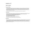
in the graph by passing its horizontal position (x) through a function. Figure 5.1
shows the four different types of graph coordinate systems that your calculator can
work with.
Whereas chapter 3 taught you rectangular or Cartesian graphing, this chapter
will introduce the other three modes in figure 5.1. We’ll first go through Parametric
113
114
CHAPTER 5
Expanding your graphing skills
Figure 5.1 The four types of graph coordinate systems your calculator
knows. At far left, Cartesian (or rectangular) coordinates, where x is
the independent variable and y(x) is the dependent variable. Parametric
mode at center-left makes both x and y dependent on a third
independent variable, t, which lets you graph functions that can’t be
expressed as Cartesian functions in the form y(x). At center-right, polar
coordinates, where the radius r is dependent on the independent
variable θ (angle). Finally, sequence graphing is for normal or recursive
functions applied to independent n values.
(PAR) mode, including some of the types of graphs it makes possible. Next, I’ll show
you Polar (POL) mode, touching on the graph variables used for polar graphing and
examples of polar functions. The third and most esoteric type of graph you’ll learn is
Sequence (SEQ) mode. With all four of the graphing modes your calculator supports
under your belt, we’ll move on to drawing.
You can annotate any kind of graph with lines, points, text, and sketches, as
you’ll learn in the latter half of this chapter. You can save annotated graphs to
later recall. Many enterprising (and bored) students have even used the drawing
tools to doodle or draw diagrams on their calculators. If you have a bunch of
graphed equations that you need to use later, you can save and recall those too, as
I’ll show you.
GRAPH STYLES ON THE TI-84 PLUS C SILVER EDITION In chapter 3, you learned to
set the color and line style of rectangular (Function mode) graphs. The same
skills apply to parametric, polar, and sequence graphs. You can change
graphs’ lines to any of 7 different styles and 15 different colors.
Let’s get started with Parametric mode, which is the closest of the three new graphing
modes to the rectangular graphing you’re now familiar with.
5.1
Parametric mode
You’ve learned all about graphing functions that map x values to y values, such as
Y1=2+X or Y2=sin(3X/5). One of the most noticeable shortcomings is that you can
have only one y value for every x value. Imagine a parabola, like the one in the left
screenshot in figure 5.2. If you were to draw a vertical line through any x value,
you’d hit only one point on the graph, whereas a horizontal line might hit zero,
one, or two points on the graph. Rectangular mode can only create graphs like
those in the left screenshot, where any vertical line crosses a graphed function at
one or zero points.
Parametric mode
115
Figure 5.2 The power of parametric graphing. Rectangular
graphing can map only one y value to each x value, meaning that
any vertical line will cross a graphed function in exactly one place
(or zero, if there is a discontinuity). Parametric mode can graph
anything Rectangular mode can, but it can also draw graphs with
multiple (or zero) y values for each x. The sideways parabola on
the right side is one such example.
The right side of figure 5.2 shows an example of what Parametric mode can do with
ease, although Rectangular mode can’t manage it. The graph shown is essentially the
equation X=(Y/2)2, which is the Y=(X/2)2 graph shown on the left turned on its side.
Parametric mode is only one of two ways to graph equations of the form x = f(y), in
addition to being able to graph circles, functions that trace over themselves many
times, and much more.
Parametric graphing in a nutshell
■
■
■
■
■
To switch to Parametric mode, press MODE , move the cursor to PAR, and
press ENTER .
When you go to the Y= menu, you’ll see pairs of functions you can enter, such
as X1T and Y1T. You must enter equations in pairs.
When you press the XTθn key in PAR, it will type a T instead of an X, because T
is the independent variable for parametric graphing.
As in normal (Function/Rectangular) mode, in Polar mode the Zoom menu options
discussed in section 3.3.1 can be used to adjust what you see in the graph.
To adjust the range and granularity of T values plugged into the parametric functions, use the Window menu.
You can see that parametric graphing is powerful, but how exactly can it do what it
does? What gives it its power? Your favorite math book or teacher can give you more
details, but the essentials are that every point in a parametric graph is defined by two
functions, not just one. In rectangular graphing, as shown on the left in figure 5.3, you
take each x value and plug it into a single function (written as y = f(x)), and the y value
pops out. By definition, each x value can have only a single y value, because a function
can’t give two different y values when the same x value is plugged in.
116
CHAPTER 5
Expanding your graphing skills
Figure 5.3 The mechanical differences between rectangular and
parametric graphing. With rectangular graphing, every y value is
generated by passing a corresponding x value through the
function to be graphed. Parametric graphing is much more
powerful because graphed functions can pass through the same
x coordinates, y coordinates, and even (x,y) point multiple times.
Parametric graphing, by contrast, defines every point on the graph by two functions;
call them x = f(t) and y = g(t). By making both x and y depend on t but not on each
other, you can express many more graphs. You can have graphs with multiple x values
for the same y, multiple y values for the same x, and even graphs that intersect with
themselves or trace over themselves.
If you have time for a longer introduction than the “Parametric graphing in a
nutshell” sidebar, let me lead you through two parametric graphing examples. The
first will show you how to graph a circle and then modify the T values plugged in to
draw a semicircle. The second exercise will demonstrate graphing a Lissajous curve
(“LEASE-a-ju”), a fancy family of graphs that can only be drawn in Parametric mode.
5.1.1
Parametric example: graphing a circle
Graphing a circle is a challenge in Function mode but surprisingly easy in Parametric
mode. It’s so easy because if you have an angle (call it t, for example) and a radius
(call it r), then the (x,y) position of the point r units from (0,0) at angle t is simply
x = r cos(t)
y = r sin(t)
Because parametric graphs work perfectly with equations for x and y that are both in
terms of a third independent variable t, you could use this to draw a circle. If you pick
a constant radius, say r = 6, and plug in every possible t (angle) value, you’ll get points
forming a circle around the origin (0,0).
You can apply this almost exactly as written to graphing a circle in Parametric
mode on your graphing calculator. Enter X1T=6cos(T) and Y1T =6sin(T), after making
sure you set your calculator to Parametric mode (see the “Parametric graphing in a
nutshell” sidebar). The equations should look like the left screenshot in figure 5.4.
Remember,
types T when you’re in Parametric mode. Press
, and your calculator should draw a circle, as illustrated on the right in figure 5.4.
Parametric mode
117
Figure 5.4 Graphing a circle of radius 6 in
Parametric mode. On the left, entering the X
and Y equations that define the circle, as
described in the text; on the right, the
results of graphing these equations.
My circle isn’t round. Figure 5.4 shows a circle that looks more like an ellipse. As mentioned in chapter 3, your calculator’s default zoom sets Xmin and Ymin to –10 and Xmax
and Ymax to 10. But because the screen is wider than it is tall, this makes circles look
stretched horizontally. You can fix this (for any Zoom setting!) by pressing
and
choosing 5:ZSquare.
If anything looks wrong, and the graph doesn’t look like the right side of figure 5.4,
press
. Choose the trusty 6:ZStandard option that even in Parametric mode
resets graph settings to sane defaults. In Parametric mode, ZStandard sets the same
graph edges as in Rectangular mode, namely Xmin = –10, Xmax = 10, Ymin = –10, and
Ymax = 10. It does something else—it sets Tmin, Tmax, and Tstep (found under
):
■
■
To graph a pair of functions like X1T and Y1T, your calculator plugs T values
between Tmin and Tmax into the pair of functions. By default, Tmin = 0 and Tmax
= 2π.
Your calculator can’t plug in every value of T between Tmin and Tmax, because
there are infinitely many. The Tstep value tells the calculator how much to add
to T each time it plugs in a new value. By default, Tstep is π/24.
You can adjust the Tmin, Tstep, and Tmax values to change how a parametric graph looks.
I’ll show you how changing Tmax can turn the circle you graphed into a semicircle.
GRAPHING A PARTIAL CIRCLE
You may recall from trigonometry or geometry that a circle is 2π radians (or 360º)
around. Because by default Tmin = 0 and Tmax = 2π, your calculator plugs all the values
necessary into your X1T =6cos(T) and Y1T =6sin(T) equations to draw a full circle of
radius 6. If a full circle is 2π, it stands to reason that half of a circle is just π. Press
, move the cursor down to Tmax=, and change the value to π (which you can type
with
). The left screenshot in figure 5.5 shows what you’ll see. Press
to set
the value, and the screen will transform into what you see in the center in figure 5.5.
Press
to graph the result: a semicircle that should match the right side in figure 5.5. Your calculator plugs in T values from T = 0 to T = π, and you get the first half
of the circle. You can change Tmin to π and Tmax to 2π if you want the other half of the
circle. You can also try making Tstep smaller and larger. Notice that if you make it
larger, the circle gets rougher, because your calculator is plugging in fewer T values.
Make it smaller, and the circle gets smoother but also takes longer to graph. If you set
it low enough, you might even be able to draw polygons!
We can revisit parabolic or projectile motion from chapter 3 with parametric
graphing, this time throwing a ball in two dimensions.
118
CHAPTER 5
Expanding your graphing skills
Figure 5.5 Modify the Window settings to graph a semicircle instead of a circle.
Press
to access the menu shown at left and center, where you can modify
Tmin, Tmax, or Tstep. Once you store your changes and press
, you’ll see
the modified graph, such as the semicircle at right.
5.1.2
Parametric example: throwing a baseball
In section 3.2.1, we used Rectangular graphing mode to look at what would happen
when you threw a ball into the air. You graphed time on the x axis and the height of
the ball on the y axis, and observed the height of the ball from the time you threw it
straight upward until it fell back to the ground. If you didn’t throw the ball straight up
but instead lobbed it across a field, the problem would get more complicated. Luckily,
because Parametric mode lets you graph x and y as a function of t, you can use it to
easily graph the path of a thrown baseball. This example will show you how.
Chapter 3 taught you that the equation for the height of a thrown ball looks
like this:
y = y 0 + v 0x + 0.5ax2
In this equation, a is the acceleration due to gravity (–9.8 meters/second2), y 0 is the
initial height of the ball when thrown, v 0 is how fast it was going (in meters/second)
when you threw it, x is time, and y is the height of the ball at time x (in seconds). If you
switch to the more intuitive variable t for time, you can use x for the horizontal position at time t and make x0 represent the starting horizontal position of the ball. If you
threw a ball across a field with an initial velocity v0, here’s what the two equations
describing its motion would look like:
x = x 0 + v 0xt
y = y 0 + v 0yt + 0.5at 2
GRAPHING A BASEBALL’S PATH
You can use these equations to graph the path of a thrown baseball over time. A professional baseball player might be able to throw a ball at 90 miles per hour, or about
40m/s. Let’s say he throws it at a 10° angle to the ground, as shown in figure 5.6. Physics and trigonometry tell us that the x-component and y-component of that initial
velocity, shown in figure 5.6, are
v 0x = v 0 cos(10°) = 40*0.985 = 39.39 m/s
v 0y = v 0 sin(10°) = 40*0.174 = 6.95 m/s
119
Parametric mode
Figure 5.6 Throwing a
baseball at a 10-degree
angle to the ground and
seeing how to calculate
the x- and y-components
of the initial velocity of
40 m/s
The math to calculate these components is shown at left in figure 5.7, along with the
equations you’ll soon enter.
You can create a pair of parametric equations describing the motion of the baseball in figure 5.6 by plugging v0x and v0y for this ball into the equations for x and y and
substituting x 0, y 0, and a as well. You may recall that acceleration due to gravity, called
either g or a, is –9.8 m/s2 (negative because it’s acceleration downward). To make
things easy, let’s assume that the ball starts at horizontal position x 0 = 0 meters, and
that if the person throwing the baseball is about 2 meters tall, the ball’s height when
he releases it is y 0 = 1.8m:
x = x 0 + v 0x t = 0 + 39.39t = 39.39t
y = y 0 + v 0yt + 0.5at2 = 1.8 + 6.95t – 4.9t2
Enter these equations as X1T and Y1T. Press
, and if there are any equations
already entered, clear them or disable them. If you don’t see pairs of parametric equation prompts, as at center in figure 5.7, go to the Mode menu and make sure you’re in
Polar mode.
DEGREE SYMBOL?
Figure 5.7 shows the degree symbol. If you want to use
sin( and cos( without specifying an angle mode in the Mode menu, you can
put the ° (degree) or r (radian) symbol after a number to specify whether it’s
a degree or radian angle. Both symbols are in the Angle menu (
).
You also need to choose a window. Because the ball starts at x0 = 0, Xmin=0 seems like a
good choice; and because the ball can’t go below the ground, Ymin=0 is also logical.
You can find the maximum y (height) the ball will reach graphically or by taking the
Figure 5.7 Calculating the x- and y-components of the baseball’s initial velocity
(left). Entering the equations for the motion of the ball for a parametric plot (center),
and a good window to see the function (right).
120
CHAPTER 5
Expanding your graphing skills
Figure 5.8 Graphing the
motion of a ball in two
dimensions versus time, on
a TI-83 Plus or TI-84 Plus
(left), or on a TI-84 Plus C
Silver Edition (right)
derivative of the expression for y. Try adjusting Ymax until you get the graph to fit well,
or take the derivative and find the roots. As a hint, Ymax=5 works well. You can also
plug in 0 for y to figure out when the ball will hit the ground, which will tell you a
good Xmax. Alternatively, you can guess and check. You’ll probably end up with
Xmax=70 or so, as shown at the right in figure 5.7.
Your resulting graph should look like one of the screenshots in figure 5.8. Because
the ball started moving with rightward and upward velocity, it curves upward before
beginning to fall again. Remember that you’re now graphing as if you were standing
in the bleachers, watching the ball’s movement. You can figure out where the ball was
at each instant by tracing over the graph. Press
, and observe the T, X, and Y values shown. Unfortunately, the calculator can’t find maxima, minima, or zeroes in
Parametric mode, so you’ll have to use the Table or calculus to figure out when the
baseball reaches the peak of its curve or when it hits the ground.
Let’s look at a third and final parametric graphing example: a fancy family of
curves called Lissajous curves.
5.1.3
Parametric example: a Lissajous curve
A Lissajous curve, also called a Bowditch curve, is a family of parametric functions created with sine and cosine. Figure 5.9 shows an example of a Lissajous curve drawn on
a graphing calculator. You can test it yourself by plugging in the two equations shown
on the left in figure 5.9, resulting in the graph shown on the right. As always, press
and choose 6:ZStandard if you don’t get the same graph.
To give you a bit of background, a Lissajous curve is any of a family of parametric
curves of the form
x(t) = a sin(ct + d)
y(t) = b sin(et)
Figure 5.9 Graphing a Lissajous curve
in Parametric mode. The left screenshot
shows the equations to enter, and the
right shows the result.
Graphing polar functions
121
In these equations, a, b, c, d, and e are constant numbers, not variables. In the example
I just showed you, we picked a = b = 8, c = 5, d = 0, and e = 3. You should try fiddling
with these variables to get different curves in the family, some of which are unique.
The keen eye might also notice that circles are technically in the Lissajous curve
family! If you let c = e = 1, d = π/2, and a = b, you’ll get a circle of radius a. You can also
graph an ellipse by keeping c = e = 1 and d = π/2 but making a and b unequal. The
semi-minor radius (the distance from the middle of the ellipse to the top or bottom)
will be equal to a, and the semi-major radius (the distance from the middle of the
ellipse to the left or right side) will be equal to b.
IMPROVING PARAMETRIC RESOLUTION
Want to make that curve look smoother? You can
apply a lesson I taught you in the parametric circle example: make Tstep smaller. Try changing
Tstep to π/48 by pressing
, changing Tstep,
and then pressing
. The curve should appear
much smoother, as in figure 5.10, although it will
take longer to render.
Parametric mode is a powerful change of pace,
great for expressing functions that are impossible
in Rectangular mode. We’ll now move on to Polar
mode, which offers some secrets of its own.
5.2
Figure 5.10 A Lissajous curve graphed
on a TI-84 Plus C Silver Edition with
Tstep=π/48
Graphing polar functions
Polar mode shares some attributes of both function and parametric graphing. As in
Function mode, single equations map an independent variable to a dependent variable. Like Parametric mode, Polar mode gives you a way to express graphs that would
be impossible in Rectangular mode and that overlap themselves.
In Polar mode, the independent variable is θ (the Greek letter theta, which represents an angle). By default, θ ranges from 0 to 2π. The dependent variable is r or
radius, a distance from the origin at angle θ. There are six polar equations, numbered
r1 through r6. Once you switch your calculator into Polar mode, as explained in the
“Polar graphing in a nutshell” sidebar, the Y= and Window menus will change to
reflect the new variables and equations.
To get you accustomed to polar graphing, let’s start with an example of the easiest
graph you can draw in Polar mode: a circle. Ironically, it’s one of the hardest things to
do in Rectangular mode, requiring two equations and careful tweaking of the ∆X variable. Polar mode plugs in θ values from 0 to 2π to any equation you enter, gets a radius,
and plots a point a distance r from the origin in the θ direction. If you enter a constant
number like 4.2 or 8 for a polar equation, then your calculator will draw a circle of that
radius. Let’s try r1=7.
The first thing you need to do is make sure your calculator is in Polar mode. Go to
the Mode menu, move the cursor to POL, and press
. You should see what the left
122
CHAPTER 5
Expanding your graphing skills
Figure 5.11 Setting Polar mode and graphing your first polar equation. The left
shows switching to POL in the Mode menu. The center screenshot displays a simple
equation to graph, and the right is the resulting circle.
Polar graphing in a nutshell
■
■
■
■
■
To switch to Polar mode, press MODE , move the cursor to POL, and press ENTER .
When you go to the Y= menu, you see six single functions you can enter, from
r1 to r6.
When you press the XTθn key in POL, it types a θ instead of an X, because θ is
the independent variable for polar graphing.
As with Parametric and Function (Rectangular) modes, the Zoom menu options
discussed in section 3.3.1 can be used to adjust what you see in the graph.
To adjust the range and granularity of θ values plugged in to the parametric functions, use the Window menu.
screenshot in figure 5.11 shows. Now press
, enter r1=7 to match the center screenshot in figure 5.11, and press
to see the result. You’ll see what the right screenshot
in figure 5.11 shows: a circle of radius 7 centered on the origin. Remember, as
we’ve discussed before, it looks like an ellipse even though it’s a circle because your
screen isn’t square.
If you wanted to fix the confusing shape of the circle, you could press
and
choose the 5:ZSquare option. In fact, for the other two examples I’m going to show
you in this section, I recommend that you use the ZSquare setting. Because polar
graphing inherently deals with circular things, it’s particularly helpful to be able to see
polar graphs in proper proportions.
Converting between polar and rectangular coordinates
Although this section teaches you to graph polar equations, you might also want to
convert between polar (r, θ ) and rectangular (x, y) coordinates. If you want to change
whether the graphscreen shows polar or rectangular coordinates when you use the
Trace feature, you can switch between RectGC and PolarGC in the Graph Format
( 2nd ZOOM ) menu.
If you have numerical (r, θ ) or (x, y) coordinates, you can convert them to the opposite
form on the homescreen using four functions from the Angle menu. All will heed your
current Radian/Degree setting in the Mode menu. Press 2nd APPS and use one
of these:
Graphing polar functions
123
(continued)
■
■
■
■
RXPr(x,y)—Computes r for the polar coordinate form (r, θ ) of the rectangular
coordinates (x, y)
RXPθ(x,y)—Computes θ for the polar coordinate form (r, θ ) of the rectangular
coordinates (x, y)
PXRx(r,θ)—Computes x for the rectangular coordinate form (x, y) of the polar
coordinates (r, θ )
PXRy(r,θ)—Computes y for the rectangular coordinate form (x, y) of the polar
coordinates (r, θ )
To help you get a feel for your calculator’s polar graphing features, I want to take you
through two examples. The first will show you how to graph a spiral, and the second
will introduce a graph called a polar rose. Let’s begin with a spiral, a surprisingly easy
shape to graph in Polar mode.
5.2.1
Polar example: a spiral
Graphing a spiral might seem rather impossible at first, but Polar mode makes it simple. If you start with a circle, which has a constant radius, then to make a spiral, you
can break the circle and pull one end into the center. A first attempt at a spiral might
be r1=θ, so that when θ = 0, r = 0; when θ = π, r = π; and when θ = 2π, r = 2π. In other
words, as θ increases, the radius r increases as well.
The initial r1=θ spiral gets very far from the origin very quickly. You can make it a
tighter spiral by dividing θ by a constant, say π, giving you r1=θ/π. The left screenshot
in figure 5.12 shows entering this equation, and the right screenshot illustrates what
happens when you press the
key (note that this screenshot was taken with
ZStandard rather than ZSquare).
That’s not much of a spiral! How can you make it continue? Remember that by
default θ goes from 0 to π, so you get only one revolution of the spiral around the origin. To create more of the spiral, you need to make θmax larger. First, press
and
change θmax to 6π. This will give you three revolutions of the spiral, which should look
much more interesting. To make the spiral look even better, switch to a square window:
press
and select the 5:ZSquare option, if you didn’t already have a square window.
Now tap
once more, and you should see the attractive graph in figure 5.13.
You can reverse the direction of the spiral by setting r1=—θ/π instead. You can make
the spiral tighter or looser by adjusting the scaling factor (here 1/π). You can modify
θmin, θstep, and θmax to see more or less spiral or to make your calculator graph a
smoother spiral. I encourage you to experiment and see what you can do with the graph.
Figure 5.12 An initial attempt at
drawing a spiral. With the default graph
settings, you get only one section of the
spiral from θ = 0 to θ = 2π.
124
CHAPTER 5
Expanding your graphing skills
Let’s examine another polar exercise: a family of graphs
that creates shapes called polar roses.
5.2.2
Polar example: polar rose
The polar rose is a family of graphs that, as you might guess
from the name, are drawn in Polar mode and look like
roses. Specifically, they’re centered on the origin and have
a number of petals. For the sake of this discussion, the general equation for a polar rose is r(θ) = a sin(bθ). The a
term controls the size of the rose and is roughly equivalent
to a radius from the middle of the rose to the tip of any
petal. The b term controls how many petals the rose has:
■
■
Figure 5.13 Your final spiral,
from θ = 0 to θ = 6π. Notice
the annotated points on the
graph, showing the (θ, r)
coordinates at several points
along the spiral.
If b is even, any rose graphed from r(θ) = a sin(bθ) has 2b petals: if b = 2, it has 4
petals, and if b = 5, it has 10 petals.
If b is odd, the rose has b petals: if b = 3, it has 3 petals, and if b = 7, it has 7 petals.
I’ll explain how you can graph polar roses, but it’s up to you to decide how many petals you want. A few of the possible roses with even numbers of petals are shown in figure 5.14.
First, pick your number of petals. Use the preceding rules about odd and even values of b to decide what value b needs to have. I recommend a radius of a = 8, but
you’re welcome to choose any radius you want. For the following discussion, I’ll
assume values of a = 8 and b = 4. Here’s how you graph the r(θ) = 8sin(4θ) rose:
1
2
3
Make sure you’re in Polar mode. If necessary, choose ZStandard and then
ZSquare from the Zoom menu to set the edges of the graph to good values.
Press
, clear out any existing equations, and enter r1=8sin(4θ). The easiest
way to type the θ variable is to press the
key, as long as you’re in Polar mode.
Press
, and your rose will appear.
As in previous exercises, I encourage you to play around with different graph settings
and values for the rose equation, if you have time. Tweak a and b to see how the rose
changes, and try varying θstep to make the rose petals smoother or rougher.
Now you’ve worked with two new graphing modes in this chapter, and you know
how to use three of the four modes your calculator offers. The fourth and final mode,
Sequence, is the least used but still powerful and handy.
Figure 5.14 Three sample polar roses, all of which have a = 8. From left to right,
b = 2, b = 4, and b = 6.
Graphing sequences
5.3
125
Graphing sequences
Sequences are special types of equations that produce successive terms, rather than a
continuous set of values. Each term of a sequence is a number, and it may or may not
depend on previous values in the sequence. Here are two simple sequence examples:
A simple sequence where terms did not depend on the values of previous terms
would be the set of positive even numbers, {2, 4, 6, 8, 10, 12,...}. If you want to
name terms of the sequence, you can call the first one u1, the second one u2,
and so on. The nth term is un, so the equation for this sequence is un = 2n: for
example, u1 = 2 and u3 = 6.
A simple sequence where terms depend on the values of previous terms would
be a sequence where each term is the sum of the previous two terms. This is a
special sequence called a Fibonacci sequence, and it starts {1, 1, 2, 3, 5, 8, 13,
21,...}. In this section, I’ll demonstrate graphing the Fibonacci sequence on
your calculator.
■
■
As in the previous discussions of new graph modes, the “Sequence graphing in a nutshell” sidebar tells you everything you need to know to quickly get started graphing
sequences. If you have time to explore two exercises with me, I’ll show you how to
graph and examine two sequences. The first will be the sequence un = n2, where each
term is the square of its index. The second sequence is the Fibonacci sequence, a classic and fun example.
Sequence graphing in a nutshell
■
■
■
■
■
■
■
To switch to Sequence mode, press MODE , move the cursor to SEQ, and press
ENTER .
When you go to the Y= menu, you’ll see one setting (nMin) and three pairs of items.
u(n), v(n), and w(n) are the sequences to be graphed, and u(nMin), v(nMin),
and w(nMin) are lists of initial values, necessary for recursive sequences.
When you press the XTθn key in SEQ, it types an n instead of an X, because n
is the independent variable for sequence graphing.
To type recursive functions, you might need to type u(n–1), u(n–2), v(n–1),
and similar expressions. The sequence equation letters u, v, and w can be typed
with 2nd 7 , 2nd 8 , and 2nd 9 , respectively.
As for every other mode, the Zoom menu options discussed in section 3.3.1 can
be used to adjust what you see in the graph. ZoomFit is particularly useful
for sequences.
The Window menu for Sequence mode has a lot of options. nMin and nMax control the range of n values that are plugged into the sequences. There’s no such
thing as nStep, because n always increases by 1. There are also settings for
the coordinates of the edges of the screen, as in every graphing mode.
The PlotStart and PlotStep options in the Window menu control which values
of the sequences are shown on the graph. This won’t change the values that are
calculated, though, which are controlled by nMin and nMax.
126
CHAPTER 5
Expanding your graphing skills
RECURSIVE A recursive sequence is one where, to find the value of the
sequence term un, you need to calculate other terms in the sequence as well.
Recursive means that to calculate those other terms, you need to find still
more terms, and the chain continues. The Fibonacci sequence we’ll examine
in section 5.3.2 is a popular series or sequence for teaching recursion.
Let’s start with the easier of our two exercises, the sequence of squares. This will give
you a good introduction on how to enter sequences and graph them, as well as how
you can use the handy Table tool to see successive values of sequences.
5.3.1
Sequence example: a sequence of squares
Sequences can range from the simple and easily understood to the very complex.
We’ll start near the easy end, with a sequence containing the squares of the positive
integers. Its equation is un = n2, so u1 = 1, u2 = 4, u3 = 9, u4 = 16, and so on. It’s particularly simple, as far as sequences go, in that you can calculate any term without knowing any other term. To calculate u9, you plug 9 into un = n2 to get u9 = 81.
Start by switching your calculator into Sequence mode, as described in the
“Sequence graphing in a nutshell” sidebar. Next, head to the Y= screen, and enter the
u(n) equation for this sequence:
u(n)=n2
Remember, the
key types the independent sequence variable n for you. As you
can see in figure 5.15, on the left, you should leave u(nMin) blank for now, because it’s
only used for a recursive equation. You might also remember from chapter 3 that the
three dots next to u(n) mean that you’re graphing this sequence as disconnected dots
instead of a line.
When you press
, you’ll see the results in the center in figure 5.15. Of course,
if you don’t have the ZStandard window set, things might look different, but choosing
6:ZStandard under the Zoom menu will swiftly fix that. Because this window is only
big enough to show three of the points in this series, you might want to adjust the window. Intuition would tell you that you need to see more of the graph above the current window, so you should increase Ymax. The right graph in figure 5.15 exemplifies
the window changed to Ymin = 0 and Ymax = 100.
Figure 5.15 Graphing a sequence of squares. On the left, entering the u(n)
equation. No u(nMin) is necessary, because the equation isn’t recursive. The
center is the result with a ZStandard window, and the right is the result with Ymin
adjusted to 0 and Ymax changed to 100.
Graphing sequences
127
USING ZOOMFIT WITH SEQUENCES
The “Sequence graphing in a nutshell” sidebar said that
ZoomFit is handy for sequences, so let’s give that a try.
Whether or not you already adjusted the window doesn’t matter; go to the Zoom menu and choose 0:ZoomFit, the tenth
item in the list. Your calculator will look at the values of nMin
and nMax, plus the values of the sequence at the u(n), v(n),
and/or w(n), and tailor a good window to the sequence(s) Figure 5.16 Using
you’ve graphed.
ZoomFit in the Zoom
Try it for this sequence: u(n)=n2. With the graph entered, menu to automatically pick
choose ZoomFit from the Zoom menu, and you’ll immedi- a good window to see part
of a sequence
ately see the result, which should look like figure 5.16. If
nMax is set to a large value, this might take a bit longer. The calculator decided to set
Xmin = nMin = 1, Xmax = nMax = 10, Ymin = u(1) = 1, and Ymax = u(10) = 100. This does a
good job of showing all the relevant terms in the sequence between n = 1 and n = 10.
EXAMINING SEQUENCE TERMS: TRACING AND THE TABLE TOOL
It’s great to visualize sequences on the graphscreen, but often you also want to know
exact numerical values of each term. As it often does, your calculator has your needs
covered. There are several ways you can get values, but two are particularly fast and easy:
■
■
Use the Trace feature—Enter one or more sequences in the Y= menu, graph them,
then press
. Use
and
to move between sequence terms; the
and
keys switch between different sequences, if you entered more than one.
Chapter 3 explains more about using Y=.
Use the Table tool—In section 3.4, you learned how to use the Table tool to see
function (rectangular) graph values. The Table tool works for all four graphing
modes and is useful for sequences. Graph one or more sequences, and then
press
. Figure 5.17 shows what the Table tool looks like for the
sequence of squares you experimented with in this section. Because the TI-84
Plus C Silver Edition has a larger screen, you may want to switch to the GraphTable split-screen mode from the Mode menu and then view the table, as illustrated on the right of figure 5.17.
Remember that if you want to change where the table starts or the spacing between
values in the table, you can adjust TblStart and ∆Tbl from the TblSetup menu,
accessed with
.
The sequence of squares I showed you in this section was a relatively easy (and
nonrecursive) sequence. You’d be missing an important piece of your sequence
graphing knowledge if you didn’t also go through a recursion exercise.
5.3.2
Sequence example: the Fibonacci series
There are endless examples of recursive functions that are useful in programming,
science, and engineering, but the Fibonacci series is a classic and easy-to-understand
example. The Fibonacci series was invented by a 13th-century Italian mathematician
128
CHAPTER 5
Expanding your graphing skills
Figure 5.17 Checking sequence values with the Table tool. After
graphing a sequence, press
to view the table. As with
normal graphing, you can modify Table tool settings from the
TblSetup (
) menu. If you use a TI-84 Plus C Silver Edition
and switch to the Graph-Table mode from the Mode menu, you’ll see
the results on the right side instead.
named Leonardo Fibonacci. It’s a sequence where the first two terms are 1, and every
subsequent term is the sum of the two terms right before it. The base cases (see the
“More on recursion” sidebar) of the Fibonacci sequence are u1 = 1 and u2 = 1, and the
recursive definition is un = un–1 + un–2:
u3 = u2 + u1 = 1 + 1 = 2
u4 = u3 + u2 = 2 + 1 = 3
u5 = u4 + u3 = 3 + 2 = 5
u10 = u9 + u8 = ? We can’t tell without calculating u9 and u8, which requires u7
and u6.
■
■
■
■
In testing the Fibonacci sequence on your calculator, you’ll learn how to enter the
expression for a recursive series, including teaching your calculator the base case(s).
We’ll explore how changing the base cases changes every other term in the series. I’ll
also reiterate the lessons about using ZoomFit to see the graphed function better and
the Table tool to get exact values.
More on recursion
■
■
Every recursive series has a definition of the recursive function. un = un–1 + n is
a definition that looks back at preceding terms. un = un+1 – n is a less-used type
of definition that looks forward at following terms.
Recursion recursively calculates values backward (or forward). Because we’d
never get values if a recursive function recursed indefinitely, recursive functions
need at least one base case. When the recursion reaches the base case, it can
stop. For example, u1 = 1 would be a useful base case for un = un–1 + n.
GRAPHING THE FIBONACCI SERIES
Just to enter the Fibonacci series in your calculator’s Y= menu, you need to learn two
new things. First, you need to learn how to refer to other terms in a series while you’re
Graphing sequences
129
writing a recursive function definition as u(n). Second, you need to know how to tell
your calculator the base cases for the recursive series.
The first problem is defining the function for the recursive series. You already
know that each term is u(n), and your calculator plugs in values for n. What if you
want to refer to the previous term, which in math notation is un–1? Use u(n–1), typed
with
. As the “Sequence graphing in a nutshell”
sidebar explains,
is the u equation,
is the n variable in Parametric
mode, and the rest is stuff you’ve seen before. If you want to refer to the term before
that, use u(n–2), and so on. For the Fibonacci example, enter u(n)=u(n–1)+u(n–2),
as shown on the left in figure 5.18.
FORWARD REFERENCES On your calculator, you can’t refer to terms after the
current term in a sequence, such as un+1 via u(n+1). This is invalid syntax. If
you try, you’ll get an ERR:DOMAIN error. You can only refer to terms before the
current term.
Next, you need to enter the base cases:
■
■
If you have one base case, you can enter it as a single number next to u(nMin)
(and v(nMin) and w(nMin), if you have two or three sequences). For example,
you could enter u(nMin)=5.
If you have more than one base case, which happens when you have a recursive
function that refers to the un–2 term or further back, you need to enter the base
cases as a list. For two base cases, you might enter {4,2}; for three, {4,2,1}.
For our Fibonacci exercise, we have two base cases: enter the list {1,1} for u(nMin),
because those are the first two terms in the Fibonacci sequence. The curly braces are
and
, as chapter 4 explained.
You have entered u(n) and u(nMin), so you’re ready to graph the Fibonacci
series by pressing
. In all likelihood, the graph won’t look quite right. An easy
fix is the ZoomFit tool we looked at in the first sequence example. Press
, and
choose 0:ZoomFit. Much better! Now you should see the plot shown on the right in
figure 5.18.
Figure 5.18 Graphing the first 10 terms of the Fibonacci series on your calculator
in Sequence mode. The left shows entering the recursive function and the base
cases. The right is the graph after you adjust the window with ZoomFit.
130
CHAPTER 5
Expanding your graphing skills
VIEWING FIBONACCI SERIES VALUES
You could trace along that graph, but an easier way to
examine the values of the series is to look at the table.
Switch into Table mode with
, and you’ll see
values of the Fibonacci sequence side-by-side with their
indices (n), as figure 5.19 illustrates. You can use the
arrow keys to scroll up and down, and you’ll soon discover that you can’t go to indices before n = 1, because Figure 5.19 Viewing the
there are no terms in the Fibonacci series before u1 = 1. table of indices and values
You can have negative indices in sequences on your calcu- for the recursive Fibonacci
lator; the lowest possible n value is whatever nMin is set to. sequence
If you want to scroll way down (or way up) the table, you
should press
and adjust the TblStart variable.
You’ve learned just about everything you need to know to use Sequence graphing
mode effectively on your calculator to explore recursive and nonrecursive series. In
fact, between this chapter and chapter 3, you know all four graphing modes that your
calculator offers: Function, Parametric, Polar, and Sequence modes. But did you know
you can draw on top of graphs and save those annotated graphs for later? Drawing
and saving graphs and graph settings are the subject of the remainder of this chapter.
5.4
Drawing on graphs
Graphing calculators are wonderful math tools. In a few seconds you can go from staring at an equation in a textbook to exploring a graph of the function, without having
to tediously draw out the graph by hand. Say you find an interesting point in such a
graph. You want to circle the point, add some text next to it to explain what it is, and
save the graph to show to your teacher later. At this point, you’ll probably end up trying to sketch the graph on a page in a notebook and annotate it by hand. After you
read this section, though, you’ll know how to draw those annotations directly on the
graph. By the end of section 5.5, you’ll also have learned how to save the annotated
graph in your calculator’s memory.
Your calculator includes a host of drawing tools, including 10 ways to draw lines,
circles, text, and even pieces of functions, and 6 ways to draw points. You can draw
directly on the graphscreen, or you can run drawing functions as homescreen functions. In this section, I’ll show you how to draw on top of graphs. You’ll learn to use
these functions directly on the graph and which ones can also be used on the homescreen. I’ll also show you the three graphing tools that are related to graphed functions: DrawInv, DrawF, and Shade(. By the time you get to the end of this section,
you’ll be well versed in drawing on your calculator. And because I’m nothing if not a
realist, I know that many of you will end up using these tools to sketch drawings of
your own. I did it too back in the day.
Let’s start with drawing functions like Horizontal, Line(, and Text( used on the
graphscreen and homescreen.
Drawing on graphs
5.4.1
131
Graphscreen drawing tools
No matter what you’re trying to draw on your calculator, from graph annotation to
geometry diagrams to doodles, your calculator has a full complement of tools to help
you. The best way to learn to use the drawing tools is to play around with them, so I’m
going to cover the high level of using the tools in general and let you experiment for
yourself. To guide you, I’ve created tables 5.1 and 5.2 (later in this section) explaining
each of the tools.
With few exceptions, most drawing tools can be used one of two ways:
■
■
Go to the graphscreen by pressing
. Optionally, you can graph equation(s)
first. From the graphscreen, press
to get to the Draw menu, pick a
tool, and use it. Continue until you’re happy with your creation.
Go to the homescreen and enter drawing commands as functions, like round(
and gcd( and all their friends. This requires memorizing the arguments to each
function, the values you put in parentheses after the function names. Chapter 2
explained how to use functions on the homescreen.
I’ll start you with drawing by example, namely graphing a parabola and annotating
that graph. We’ll then touch briefly on homescreen drawing commands and conclude
this section with a table of the drawing tools you’ll use most frequently. If you have a
TI-84 Plus C Silver Edition, you may also want to refer to section 12.3, which discusses
the differences between drawing on the older and newer calculators.
USING DRAWING TOOLS ON THE GRAPHSCREEN: ANNOTATING A PARABOLA
The easiest way to draw on your calculator is to use its drawing tools directly on the
graphscreen. You can draw lines, circles, text, points, and more. To select any drawing
tool, start on the graphscreen, press
to access the Draw menu, and pick
the tool you want. The Draw menu has three tabs—DRAW, POINTS, and STO—as you
can see from figure 5.20. You’ll learn about the STO tab in section 5.5. On the TI-84
Plus C Silver Edition, there’s a fourth tab called Background, but you won’t need to
use that unless you’re writing a program.
When you pick a drawing tool from the Draw menu, that tool will remain active
until you pick another one. You can draw multiple lines, circles, strings of text, and
more without needing to keep reselecting the same tool from the Draw menu. You’ll
use that technique in this section’s example: annotating a parabola.
Start with a parabola by switching to Function mode (by accessing the Mode
menu), entering Y1=5–(X–2)2 in the Y= menu, and pressing
. Doesn’t look like
figure 5.21? No problem; go to the Zoom menu, and choose 6:ZStandard. You can
Figure 5.20 The DRAW and POINTS
tabs of the Draw menu, containing
general tools (left) and point-drawing
tools (right). The STO tab contains ways
to save and restore graph settings and
pictures, as you’ll see in section 5.5.
132
CHAPTER 5
Expanding your graphing skills
Figure 5.21 Graphing a parabola and annotating it. PEAK and PARABOLA are drawn
with the Text tool, the circle is a Circle, and the arrow is three Lines. The left
side shows the equation, and the middle shows the graph before being annotated.
always turn the axes on and off and modify other graph format options using the
keys.
Now let’s try some annotations:
1
2
3
4
Try circling the peak. From the graph, press
to open the Draw
menu, and scroll down to 9:Circle(. Move the cursor over the peak, press
to set the circle’s center, and then move the cursor to a point where you
want the edge of the circle to be and press
again. A circle!
Write out PEAK, as in figure 5.21. Go to 0:Text( in the Draw menu, and then
use the arrow keys to move the cursor. Place it at the top-left corner of where
you want the word PEAK to appear, and type PEAK. Remember that to type a
string of letters, you press
to engage Alpha-Lock, and then press the
keys that have the letters you want printed over them.
You can type PARABOLA without returning to the Draw menu. Move the cursor to
a new position with the arrow keys, and type PARABOLA.
Create the arrow pointing to the parabola in figure 5.21. Go to the Draw menu, and
select the 2:Line( tool. For each line, move the cursor to the first endpoint, press
, move the cursor to the second endpoint, and press
again. The tool you
select stays active until you select another tool, so you don’t need to return to the
Draw menu before each new line. The arrow in figure 5.21 is three lines.
While you were drawing, you might have been frustrated that the coordinates at the
bottom of the screen were getting in your way. If you don’t mind them while you’re
drawing, but you want them to go away when you finish drawing, press
. Don’t
worry; it won’t clear the screen. At worst, you might accidentally quit to the homescreen, at which point you need only press
to return to the drawing. If you don’t
want coordinates to show at all while you draw, select CoordOff from the Graph Format menu,
. If you’re on a TI-84 Plus C Silver Edition, you could press
in the middle of drawing any shape to access the Style menu, as indicated by the
onscreen Style button above the
key.
CLEARING THE GRAPHSCREEN: CLRDRAW
The 1:ClrDraw command from the Draw tab of the Draw menu clears the entire
graphscreen. If you have the axes or grid enabled, it redraws them as well and then
rerenders any functions you’ve graphed. Press
, and then go to the Draw menu
Drawing on graphs
133
with
, and choose 1:ClrDraw. If you’re on the homescreen, you can enter
ClrDraw as a command on a line by itself and press
.
Be aware that zooming a graph, panning left or right, changing the window, or
changing or removing an existing graphed function will also erase the graphscreen.
Adding a new function will not erase annotations you’ve drawn, as long as you don’t
change existing functions.
SKETCHING ON A BLANK SCREEN Want a blank screen for your doodles, diagrams,
and sketches? Turn off the axes and grid by making sure AxesOff and GridOff
are selected in the Graph Format menu, under
. Don’t forget how to
turn them on again if you need to graph, but remember that graphing and modifying Graph Format options will erase anything you’ve already drawn!
5.4.2
Using drawing tools on the homescreen
It’s easy to use your calculator’s drawing tools on the graphscreen, but sometimes you
need more precision than you can get by using the tools directly on the graphscreen.
Or perhaps you need to draw lines or circles that are partially offscreen. In this case,
you’ll want to use the drawing tools from the homescreen.
Let’s go through an exercise, because that’s the easiest way to learn anything.
You’ll draw a circle, a horizontal line, and a vertical line from the homescreen. Here
are the steps:
1
2
3
4
Remove any equations from the Y= menu. You can also turn off the axes with
AxesOff from the Format menu (
) if you want. You may want to use
ZStandard and then ZSquare from the Zoom menu to make your results match
my screenshots.
Use ClrDraw from the Draw menu to start with a blank graphscreen.
From the homescreen, issue the commands Circle(2,4,10) to draw a circle
centered at (2,4) of radius 10; you can see the command in figure 5.22 or
figure 5.23. If you’re using a TI-84 Plus C Silver Edition, use the command
Circle(2,4,10,RED); you can find RED under
.
Use the Horizontal —6 and Vertical —8 options to draw two lines tangent to the
circle. You should see something that matches the right side in figure 5.22 or
figure 5.23. If you have a TI-84 Plus C Silver Edition, try Vertical —8,GREEN
instead of Vertical —8.
Figure 5.22 Using drawing commands from the homescreen to draw a circle, a
horizontal line, and a vertical line. For this example, I turned off the axes with
AxesOff and used ZStandard and ZSquare to set up the window.
134
CHAPTER 5
Expanding your graphing skills
Figure 5.23 The same set of drawing commands as figure 5.22 on the TI-84 Plus
C Silver Edition. I used colors in two of the commands, found in the Color tab of the
Vars menu.
For the full list of drawing commands, look at tables 5.1 and 5.2. Table 5.1 contains
most of the interesting commands from the Draw menu, and table 5.2 lists the commands from the Points tab.
Table 5.1 Drawing functions in the Draw tab of the Draw menu. You must first go to the graphscreen,
press
and select the function you want, and then use it. You can also go to the
homescreen instead to use many of these functions. If you have a TI-84 Plus C Silver Edition, you should
instead refer to table 12.2 in section 12.3.
Command
What it does
Homescreen syntax
Draws a line between two points.
On the graphscreen, move the cursor
to the first point, press
; move
it to the second point, and press
again.
Line(<x1>,<y1>,<x2>,<y2>)
Horizontal
Draws a horizontal line across the whole
screen. Move the line to where you want it,
and press
to make it permanent.
Horizontal <y coordinate>
Example: Horizontal 1.5
Vertical
Draws a vertical line down the whole
screen. Move the line to where you
want it, and press
to make
it permanent.
Vertical <x coordinate>
Example: Vertical —4
Tangent(
Draws a line tangent to a given function at a
given x point. Always assumes that functions
are rectangular (FUNC) functions, even if the
calculator isn’t in Function mode. On the
graphscreen, you select the function and
then the point.
Tangent(<func>,<x coord>)
Example: Tangent(3X2,1.25)
Circle(
Draws a circle with a center and radius. On
the graphscreen, select the center, press
, and then choose a point on the edge
of the circle.
Circle(<center >,
<center y>,<radius>)
Example: Circle(2,—1,4)
Line(
Example: Line(—1,0,8.2,8)
135
Drawing on graphs
Table 5.1 Drawing functions in the Draw tab of the Draw menu. You must first go to the graphscreen,
press
and select the function you want, and then use it. You can also go to the
homescreen instead to use many of these functions. If you have a TI-84 Plus C Silver Edition, you should
instead refer to table 12.2 in section 12.3. (continued)
Command
What it does
Homescreen syntax
Text(
Writes out text. Move the cursor where you
want the top-left corner of the text to be, and
start typing (no need to press
).
Remember to press
if you want to
type letters. For entering Text( on the
homescreen, row and column are pixels from
the top-left of the screen, which is row 0,
column 0. The bottom-right is row 62,
column 94.
Text(<row>,<column>,
"STRING")
Example: Text(57,1,"GRAPH
TITLE")
Pen
Somewhat like drawing with an Etch-aSketch. Move the cursor to where you want
to start, press
to put the “pen” down,
and move the “pen” to draw a black line
behind it. You can press
to lift
the “pen” and move it to a new spot to
draw again.
(You can’t use the Pen as a homescreen command.)
Table 5.2
Point and pixel commands, all in the Points tab of the Draw menu
Command
What it does
Homescreen syntax
Pt-On(
Pt-Off(
Pt-Change(
Once you enable this tool, you can freely
move the cursor around the graphscreen.
Every time you press
, it will turn the
point on (to black), turn it off (to white), or
change it. From the homescreen, this command uses (x,y) coordinates. If you omit
<type>, it draws a single dot. You can
enter 2 for type for a square and 3 for
a cross.
Pt-On(<x>,<y >,[<type])
Pt-Off(<x>,<y >,[<type])
Pt-Change(<x>,<y>,[<type])
Example: Pt-On(5,1.2)
Pxl-On(
Pxl-Off(
Pxl-Change(
Can’t be drawn on the graphscreen;
only for use as a homescreen function.
Like Text(, takes pixel coordinates.
Row and column are pixels from the
top-left of the screen, which is row 0,
column 0. The bottom-right is row 62,
column 94.
Pxl-On(<row>,<column>)
Pxl-Off(<row>,<column>)
Pxl-Change(<row>,<column>)
Example: Pxl-Off(30,52)
There are three more drawing commands that we haven’t discussed yet in the Draw
tab of the Draw menu, all of which work with graphed equations. You’ll learn how to
use those before we move on to the final topic of the chapter, saving and restoring pictures and graph settings.
136
5.4.3
CHAPTER 5
Expanding your graphing skills
Drawing graphlike functions: DrawInv, DrawF, and Shade
Three of the tools in the Draw menu (
) take functions as arguments and
draw something based on equations. All three work only in Function mode or act as if
the calculator is in Function mode regardless of the current settings. These three
functions are as follows:
DrawInv—Draws the inverse of a Y= rectangular equation. Useful for drawing X=
■
equations (see the “Graphing X= equations” sidebar for more information).
This function takes one argument: the equation to graph the inverse of. For
example: DrawInv X2+3.
DrawF—Graphs a function, just as if you had entered it in the Y= menu. This
function works only with rectangular/function (Y=) equations, even if the
graphing mode is set to one of the other modes. Like DrawInv, it takes a single
argument: an equation to graph. For example, DrawF √(X) would be equivalent
to setting Y1=√(X).
Shade—Draws a solid or hashed shade between two functions (or y coordinates).
It takes at least two arguments: the two functions (or y coordinates) bounding
the shaded area. For example, Shade(X2,10) shades the area between y = x2 and
y = 10 in solid black. You can also choose minimum and maximum x coordinates
on the shaded area, so Shade(X2,10,0,2) only shades between x = 0 and x = 2.
■
■
Graphing X= equations
Many graphing-calculator users struggle to find a way to graph equations of the form
x = f(y), such as x = y2 or x = 1 + 5sin(y). If you’re looking for a way to graph X= equations, there are two possible methods:
■
■
DrawInv—If your calculator is already in Function (Rectangular) graphing mode,
use the DrawInv command from the Draw menu. DrawInv takes one argument:
the function to graph, with Ys replaced by Xs. In other words, DrawInv X2 draws
the equation x = y2.
Parametric mode—Take your x = f(y) equation, such as X=1+5sin(Y), and
replace the Ys with Ts. Enter your equation as x1T, such as X1T =1+5sin(T), and
set Y1T =T. You’ll also need to adjust Tmin to Ymin and Tmax to Ymax.
Except for DrawInv’s use as a way to graph X= equations, you probably won’t find yourself using these three tools that often. Nevertheless, for the sake of completeness, I’d
like to show you a brief exercise that uses all three of these drawing tools. You’ll use
DrawF and DrawInv to graph Y=3sin(X) and X=3sin(Y) and then shade between
Y=3sin(X) and Y=3sin(X)–3 using the Shade( command.
To set up, press
and change your calculator to Function mode, if it’s not
already in it. Turn on the axes from the Graph Format menu (
) if they’re
not already on, and select 6:ZStandard from the Zoom menu. Finally, if you still
have anything on the graphscreen, clear any entered equations from the Y= menu,
Saving graph settings and pictures
137
Figure 5.24 Using the DrawF, DrawInv, and Shade( commands. The left shows
the three commands to enter, the center shows the effect of just DrawF and
DrawInv, and the right is the result after the Shade( command.
and, if necessary, select 1:ClrDraw from the Draw menu (
these steps:
1
2
3
). Next, follow
Select 6:DrawF from the Draw menu, and add 3sin(X) as an argument. You’ll end
up with DrawF 3sin(X), as in figure 5.24. Press
to execute the command.
Choose 8:DrawInv from the Draw menu, and add 3sin(X) again, to get DrawInv 3sin(X). This graphs x = 3sin(y); from the DrawF and DrawInv commands,
you’ll get the screenshot in the center of figure 5.24.
Use the Shade( command from the Draw menu to shade between y = 3sin(x) – 3
and y = 3sin(x) with Shade(3sin(X)–3,3sin(X)). Press
, and when the calculator finishes drawing, you’ll see something that resembles the right side of
figure 5.24.
As with all the other drawing tools, and in fact nearly every skill you’ve learned so far, I
encourage you to experiment with these three new drawing features to see how they
can help you with your academic work and your own drawings. But what if you want to
save the results of your drawing efforts? In the next section, you’ll learn to store snapshots of the graphscreen and restore them, as well as save and restore graph settings
for later use.
5.5
Saving graph settings and pictures
The final skills of this chapter are among the easiest of the new graphing and drawing
skills, and thus I saved them until the end to relax your brain after the rigors of graphing and drawing. In addition, there’s no point saving pictures of the graphscreen and
your graph settings if you have neither graphs nor pictures. In a nutshell, this section
will show you how to take a snapshot (or picture or screenshot, if you prefer) of the
graphscreen and save it into your calculator’s memory. You can later restore one of
those pictures to return the graphscreen to how it looked when you took the picture,
regardless of any new graphs, drawings, mode changes, and format changes that you
made in the meantime. This section will also explain graph databases (GDBs), a way to
store all currently graphed equations plus your Graph Format settings and graph window into memory. You can then later restore a GDB to return your graphs and settings
to the way they were when you stored the GDB.
Saving and recalling pictures (pics) is useful whenever you’ve made an annotated
graph or a drawing that you want to store for later. Pictures are the first topic we’ll
138
CHAPTER 5
Expanding your graphing skills
examine. The second is saving and recalling GDBs, which is handy when you have your
graphed functions and graph format settings exactly as you want them and want to be
able to later switch back to those settings.
Let’s get right to it with a look at your calculator’s picture variables and features.
5.5.1
Saving and recalling picture variables
Just as your calculator has numerical variables for storing numbers, list variables for
storing lists, and matrix variables for storing matrices, it has a set of 10 picture variables for storing pictures or snapshots of the graphscreen. Named Pic1 through Pic9
plus Pic0, each is a location in your calculator’s memory, and each can store a full
image of the graphscreen.
In section 5.5.1, I refer to “Pic1 through Pic9
plus Pic0” instead of just saying “Pic0 through Pic9.” This isn’t an error or an
attempt to confuse you. Because your calculator thinks of Pic0 as Pic10, it’s
the last of the 10 picture variables, after Pic9.
WHY NOT PIC0 THROUGH PIC9?
The StorePic and RecallPic commands, which
respectively store and recall picture variables,
can be found in the STO tab of the Draw menu.
To access this menu, shown in figure 5.25, press
. Once you choose StorePic
or RecallPic, the command is pasted to the
homescreen. Add a 1, 2, 3, ..., 9, or 0 after either
StorePic or RecallPic to save or open that picture number.
Figure 5.25 The STO tab of the
Draw menu, from which you can save
and recall both pictures and graph
settings (GDBs)
PICTURE CAVEATS If you StorePic a picture
that already exists, your calculator will overwrite the old picture without warning you. If you try to RecallPic a picture that doesn’t exist, your calculator
will show an ERR:UNDEFINED message.
If you want to see a list of which picture variables you have on your calculator, you can
press
to access the Memory menu, then choose 2:Mem Mgmt/Del…, and
choose 8:Pic…. You’ll see a list of any picture variables on your calculator, and you can
archive, unarchive, and delete pictures from here. Press
next to any picture to
delete it, which saves memory (RAM). If you archive a picture by pressing
next to
it, which adds an asterisk (*), then it won’t take up RAM and will survive a RAM clear.
But you can’t StorePic or RecallPic that variable until you unarchive it by returning
to the Memory menu and pressing
next to it again.
To demonstrate saving and recalling pictures, I drew a sketch on the graphscreen,
as shown on the left in figure 5.26. Next, I cleared the graphscreen with ClrDraw and
then recalled the picture that I saved, as shown in the center in figure 5.26. When I
pressed
, the sketch I had drawn was restored.
Saving graph settings and pictures
139
Figure 5.26 Demonstrating how StorePic and RecallPic let you save a
snapshot of graphs, annotations, or drawings on the graphscreen. Here, I store the
DNA doodle I drew, clear the screen (erasing the doodle), and then use RecallPic
to restore the sketch.
What if you want to save not the exact contents of the graphscreen but the equations
that you have currently graphed, plus the window and format settings? Then you
should use a GDB.
5.5.2
Saving and recalling graph databases
A graph database, or GDB, is a somewhat different animal than a picture variable.
There are 10 of them, GDB1 through GDB9 plus GDB0, and they’re located in your calculator’s memory. But instead of holding an exact snapshot of the pixels on the graphscreen, GDBs hold all the following:
■
■
■
■
■
Any equations you have entered in the Y= menu, for all four modes.
The current graph mode.
The Graph Format settings from the Format menu, including whether the axes,
the grid, and coordinates are on or off.
The window variables, including Xmin, Xmax, Ymin, Ymax, and any other values
in
.
On the TI-84 Plus C Silver Edition, it also saves the colors of each graphed equation, the axes color, the grid color, and the color of the border around the
graph. It does not save the background picture or color.
Saving and recalling GDBs use the StoreGDB and RecallGDB functions from the STO
tab of the Draw menu, as shown in figure 5.25. You follow StoreGDB and RecallGDB
with a number from 0 to 9, exactly as with StorePic and RecallPic. I showed you how
to list the picture variables on your calculator and archive and delete them from the
Memory menu. You can list, delete, and archive the GDB variables nearly the exact
same way: press
to access the Memory menu, then choose 2:Mem Mgmt/Del…,
and choose 9:GDB….
Figure 5.27 shows an example of storing a GDB, messing with Graph Format settings and graphed equations, and then recalling the original GDB. By recalling GDB4,
the initial set of functions and settings from the left in figure 5.22 is restored, undoing
the changes I made to the graph format and the window settings.
And now we’ve reached the end of what you need to know for advanced usage of
your calculator’s drawing and graphing features! From here on, we’ll focus on advanced
140
CHAPTER 5
Expanding your graphing skills
Figure 5.27 Starting with the graph on the left, the StoreGDB 4 command
stores the graphed equations and graph settings to graph database GDB4. After I
turn the axes off and the grid on and change the window settings, the graph
changes to what you see in the center. The RecallGDB 4 command restores it
to the right view, just as it was when the StoreGDB 4 command was issued.
math features, although some of the discussion, such as statistics, will include use of
plots and graphs on the graphscreen.
5.6
Summary
In this chapter, you learned advanced skills for graphing and drawing. We started with
the three graphing modes that chapter 3 didn’t explore: Parametric mode, Polar
mode, and Sequence mode. You learned how Parametric mode lets you express and
graph functions that would be impossible in Function or Rectangular mode. You
explored examples of polar functions, from circles and spirals to rose-shaped graphs.
We worked through sequence graphing exercises of a recursive series like the Fibonacci series and a nonrecursive series like the squares of the positive integers.
In the latter half of the chapter, I showed you the many drawing and annotation
tools that your calculator offers. From ways to mark up graphed equations to shade
functions and graph X= equations, there’s not much you can’t draw on your calculator’s graphscreen. You even learned how you can use the graphscreen as a creative
canvas for freehand sketches and diagrams. We concluded with a look at the tools for
storing and recalling pictures, which store the pixel-by-pixel contents of the graphscreen; and GDBs, which hold the currently graphed equations and graph settings.
As we move forward into the rest of part 2 of this book, you’ll be graduating to the
realm of precalculus and calculus. Chapter 6 focuses on precalculus features of your
graphing calculator that you haven’t explored yet. You’ll look at complex numbers,
the nitty-gritty of trigonometry, limits, and logarithms. Onward!
MATHEMATICS/GENERAL
Using the TI-83 Plus/TI-84 Plus
Full Coverage of the TI-84 Plus C Silver Edition
Free eBook
see insert
Christopher R. Mitchell
W
ith so many features and functions, the TI-83 Plus/
TI-84 Plus graphing calculators can be a little intimidating. This book turns the tables and puts
you in control! In it you’ll find terrific tutorials that guide you
through the most important techniques, dozens of examples
and exercises that let you learn by doing, and well-designed
reference materials so you can find the answers to your questions fast.
Using the TI-83 Plus/TI-84 Plus starts by making you comfortable with these powerful calculators’ screens, buttons, and
special vocabulary. Then, you’ll explore key features while you
tackle problems just like the ones you’ll see in your math and
sciences classes.
“ The user manual—but shorter,
clearer, and much more
entertaining!”
— Louis Becquey, Joseph Fourier
University, Grenoble
“Expertly captivates readers at
any level of study, and provides
practical examples that students
will use in their academic years
and beyond.”
— Samuel Gockel, University of
Illinois at Urbana-Champaign
What’s Inside
Get up and running with your calculator fast!
● Lots of examples
● Special tips for SAT and ACT math
● Covers the color-screen TI-84 Plus C Silver Edition
●
Written for anyone who wants to use the TI-83 Plus/TI-84 Plus.
No advanced knowledge of math and science required.
Christopher Mitchell is a teacher, PhD candidate, and recog-
nized leader in the calculator enthusiast community. You’ll find
Christopher (aka Kerm Martian) and his cadre of calculator
experts answering questions and sharing advice on his website,
cemetech.net.
To download their free eBook in PDF, ePub, and Kindle formats, owners
of this book should visit manning.com/UsingtheTI-83Plus/TI-84Plus
MANNING
US $24.99 / Can $26.99
“ The perfect complement to math
and statistics courses of all levels.”
— Ryan Boyd
University of Texas at Austin
“ This is THE manual for your
calculator.”
— Jonathan Walker, computer science
student, NDSU