Download Text (Revised 22.10.2012)

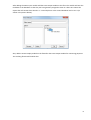
Refraction Seismic Survey Data Processing in
RadExPro Using the Easy Refraction Module –
Practical Guide
(Revised October 22, 2012)
DECO Geophysical SC OOO
Moscow State University Science Park,
1-77 Leninskie Gory
Moscow 119992, Russia
Tel./Fax: (+7 495) 930 94 14
E-mail: [email protected]
Website: www.radexpro.com
1
Contents
Contents......................................................................................................................................................2
Introduction.................................................................................................................................................2
Creating a project........................................................................................................................................2
Data loading and geometry assignment......................................................................................................6
First arrivals picking...................................................................................................................................12
Working with the Easy Refraction module.................................................................................................15
Identifying travel time curve fragments related to different layers.......................................................17
Automatic travel time inversion............................................................................................................19
Manual travel time inversion................................................................................................................20
Exporting the results.............................................................................................................................23
Introduction
This Guide is intended for users making their first steps in refraction seismic survey (RSS) data processing
in RadExPro using the Easy Refraction module. The Guide covers all processing stages – from data
loading and geometry assignment to first arrival picking, identification of travel time curve sections
corresponding to different layers, and, finally, travel time inversion and generation of a layered velocity
model of the medium.
It is assumed that the user is already familiar with the theory behind RSS and the t0 method.
Source data as well as the project that should be generated as a result of completing this tutorial can be
downloaded from our website: http://www.radexpro.com/downloads/tutorials
Creating a project
A project is a combination of source data, intermediate and final processing results, and
processing flows organized into a common database used by RadExPro seismic data processing package.
Projects are stored in separate directories on the hard disk. When a new project is created, a project
directory is automatically created for it. Projects can be moved between computers by simply copying
the appropriate directory (provided that all used data are stored within that directory).
Launch the project manager by opening the Windows Start Menu and selecting All
Programs/DECO Geophysical/RadExPro 2011.2.
2
Launching the project manager opens a dialog box with a list of registered projects.
Click the New Project button and select a parent directory on the hard disk where the project
subdirectory will be created. Another dialog box will appear, prompting you to enter a project name.
Make sure that the Create subfolder option is checked and press Ok. A subdirectory with the
same name as the project will be created in the selected directory. The project will also appear in the list
of available (registered) projects.
3
Select the project and press Ok.
This will open the main RadExPro window containing the project tree.
Before starting to work on the project, we recommend creating a directory called data within the
project directory and copying all data to it. Although this step is optional (data located outside the
project can also be read), storing the data within the project directory allows the program to use relative
file paths rather than absolute ones. This makes project migration from one computer to another easier.
4
The RadExPro database has 3 structural levels. The upper level corresponds to the project area,
the middle level – to the line, and the lower level – to the processing flow. Right-click the yellow circle,
select the Create new area option, and enter a name for the project area.
5
The picture below shows the dialog box prompting you to enter the area name:
In a similar manner, right-click the yellow rectangle with the area name, select Create line, and
create a new line.
Enter the line name just like the area name.
The database allows storing several areas within one project and several lines within each area.
Each line is processed by several flows.
6
Data loading and geometry assignment
Create a processing flow named 010 – data load in the same manner as you created the area
and the line.
Switch to the flow editing mode by double-clicking the flow name with the left mouse button.
This will open the flow editor window where we will now create a flow consisting of the SEG-Y Input and
Trace Output modules.
Specify the data reading parameters when adding the SEG-Y Input module.
7
After adding the SEG-Y Input module add the Trace Output module to the flow. This module will save the
read data to the database so that they can have geometry assigned to them at a later time. Name the
object that will contain these data line 1 – raw and place it at the second database level in Line 1 (as
shown in the picture below).
Also, add the Screen Display module to the flow after the Trace Output module for monitoring purposes.
The resulting flow should look like this:
8
Select the Run menu item to run the flow. The Screen Display window showing the data being
entered will open, and the data themselves will be read from the file on the hard disk and saved to the
database. The Screen Display window that should appear on the screen is shown below.
9
Now we need to assign the geometry – source coordinates (SOU_X) and receiver coordinates
(REC_X) – to the seismic data. We will use Near-Surface Geometry Input module for that.
Create a new flow: 020 – Geometry Input, add Trace Input module, select the raw_data dataset
that we have created before and load all traces in the order they are stored in the dataset (for that chose
Get all option of the Trace Input).
10
Now we can add Near-Surface Geometry Input module to the flow. The module is dedicated to
assigning geometry to seismic data acquired using different techniques typical for near-surface
applications, including conventional refraction acquisition scheme.
When the module is added to the flow, you will see its parameter dialog as shown below. For assigning
geometry to seismic refraction data select the Refraction tab of the dialog:
11
Our sample data was acquired according to the following scheme: our receiver streamer contained 48
geophones equally spaced every 1 meter. Shots on the streamer were made on channels 1, 12, 24, 36
and 48 (0, 11, 23, 35, 47 m accordingly). Offset shots we made 24 meters ahead of the 1 st channel and 23
meters behind the last channel.
In case of refraction data, the module will calculate and assign shot point coordianates (SOU_X), receiver
coordinates (REC_X), and source-receiver offsets (OFFSET) based on shot point numbers (FFID) and
channel numbers (CHAN). For correct geometry assignment we will specify the following parameters:
Receivers:
•
First receiver position – 0
•
Receiver step – 1
•
Number of channels – 48
Streamer sources
12
Let us specify each source position manually. Select Variable step option to see the table with the shot
point numbers and their coordinates. Set Number of sources to 5 and type their coordinates into the
table: 1-0, 2-11, 3-23, 4-35, 5-47.
Offset sources
Select Variable step option, set Number of forward sources to 1 and type in the coordinate of -24 m.
The same way, set Number of reverse sources to 1 and type in the last shot point coordinate of 70 m.
! This data was acquired in such a way that the original field channel numbering is not sequential (1, 25,
2, 26, etc. – a result of some technical peculiarities of the receiving system). However, for correct
geometry assignment we need the channels and shot points to be numbered sequentially, in the order
they were acquired in field. To correct the numbering we switch on Reassign FFID and CHAN headers
option. This would recalculate and reassign all shot point numbers and channel numbers according to
the order the traces input the module in the flow.
Finally, the dialog shall look as shown below:
When the parameters are set, click the OK to save your settings.
Now we will add Trace Output at the end of the flow to save the data with assigned geometry to a new
dataset in the project database. We will call the new dataset geom_data and place it at the Line 1 level
of the database (as shown below):
13
The resulting flow shall look as following:
Now click Run in the menu to execute the flow. As a result we will have a copy of the data with
geometry assigned.
First arrival picking
Create a new flow named 030 – Picking and add the Trace Input module to it. After that add the newly
created dataset to the Data Sets window and apply sorting by SOU_X and REC_X to the entire selection.
14
Then add the Screen Display module, selecting trace image scales and amplification factors suitable for
first arrivals picking. Additional processing procedures – such as Bandpass Filtering, Hand Static etc. –
can be enabled as necessary. However, you should keep in mind that filtering (especially zero-phase)
“blurs” first wave arrivals; therefore, first arrivals picking should be done before filtering.
In the Screen Display dialog set the following parameters:
Click the Axis button and set the following axis parameters:
15
Run the flow and see the data as shown below.
Select the Tools/New pick menu item and perform first arrival picking. After that you can pick first
arrivals or extremums. Use zoom/unzoom buttons on the toolbar to select convenient scale.
You can select the mode of picking in the Picking parameters dialog achieved through the
Tools/Pick/Picking parameters menu item.
16
Picking can be done manually (Mode: Manual) or using on of the semi-automatic modes (Auto fill or
Hunt). In the Auto fill mode the program automatically tracks selected event between two interpreter
pick nodes according to the specified Parameters. In the Hunt mode it would try to follow the specified
event in either one or both directions from the initial pick until it looses correlation.
To perform picking, click the left mouse button when the mouse cursor is over the selected point. An X
mark will appear at that point showing a pick node. Click the left mouse button once more within the
same trace to move the node to a new position, or click within another trace to place a new node. An
erroneously placed node can be removed by right-mouse button double-click or moved to a new
position by drag-and-drop with the right mouse button.
You need to pick all seismograms. To save the pick, select the Tools/Save As… menu item or right click on
your pick in the Pick List window and select the same Save As command from the pop-up menu.
17
This will open a dialog box where you will be asked to enter the pick name and specify which database
object the pick will correspond to by left-clicking the appropriate object.
The program also allows saving travel time curves as text files for further use in other interpretation
software (Tools/Pick/Export pick).
Press Pick headers… and make sure that SOU_X is selected in the left column and REC_X – in the right
column.
18
Working with the Easy Refraction module
Create a new flow named 004 – Easy refraction and add the Easy Refraction module to it. Select
Browse… in the dialog box.
This will open another dialog box prompting us to specify the “scheme” name. An “Easy Refraction
scheme” is a combination of travel time curves (possibly divided into segments) corresponding to
different layers generated as a result of boundary processing etc. When the user exits the module, its
current state is stored in the “scheme”.
After entering the new scheme name, press Ok and run the flow.
The Easy Refraction module working window will open.
19
Press the Load time curves button to load travel time curves. This will open the travel time curve
selection window. Load the necessary time curves and press Ok.
The module window containing the loaded travel time curves will appear.
20
You can make a number of manipulations with the time curves here: edit nodes, smooth them,
interpolate, move etc. Refer to User Manual for the details.
As an example of such a manipulation we will mirror one of the curves. When we were picking fist
breaks, the data from the first shot (at -24 m) was noted to be of very poor quality, so it was difficult to
make a reliable pick. So now, if you have created a pick at the shot point -24, delete it (click of the pick in
the list of picks in the left pane of the window and press Delete key on the keyboard). We will substitute
this pick with a mirrored pick from the shot point at 70 m (although we need to understand that this is
not 100% fair procedure, of course). For that, switch off all time curves except of the one from shot point
70 m, select it with the left mouse button and select Time Curves/Mirror curve. As a result we will have
a symmetrical time curve tied to SP -23 m:
21
Identifying travel time curve fragments related to different layers
We need to mark travel time curve fragments related to particular layers. Let us do this using the
interactive marker.
Select the Time Curves/Marker/1 menu item or press 1 on the keyboard. You will see a pink circle of the
marker of the fist layer. You can change its diameter by rotating the mouse wheel while keeping Shift key
pressed.
Press and hold the left mouse button to mark the travel time curve sections related to the first layer. The
interpreter selects travel time curve breakpoints and determines the number of layers in the section
interpretation model according to the principles described in the literature. Linear approximation as well
as output of resulting velocity values per travel time curve is done automatically.
22
Similarly, select the second marker and mark the travel time curve sections related to the second layer.
Visualization of individual travel time curves can be disabled by unchecking the appropriate boxes in the
left pane of the module.
To exit the marker mode, open the Time Curves/Marker/2 menu item and left-click (or press the ` key
on your keyboard) to uncheck it.
Automatic travel time inversion
With the Easy Refraction you can invert travel time curves either automatically, or manually. We will
check both methods below.
For automatic inversion (prior layer selection with the marker is required) select Inversion/Automatic
inversion menu command (you can also press F5 or click on the green arrow on the toolbar).
The results are shown in the picture below: the position of the boundary between the first and the
second layer has been built in the lower part of the module working window. Velocities above and below
the boundary are colorcoded.
23
Press t key to show/hide layer velocity values at the section.
Manual travel time inversion
If necessary, all refraction processing stages can be carried out manually with the full controll over the
intermediate results.
The module allows building the difference between two travel time curves. To do this, select one travel
time curve with the left mouse button, another one – with the right mouse button, and open the Time
Curves/Travel time difference menu. A graph showing the difference between the two selected travel
time curves will be built in a separate window. If diving waves are registered in the first arrival, the entire
difference graph will be a decay function; if head waves are registered, the function will decay at first,
but then will become constant.
24
The module allows building composite travel time curves – time curves of waves from each refraction
boundary. This procedure is necessary to obtain a travel time curve covering the “dead zone” – the direct
wave tracking area on the direct and opposite travel time curves. The head wave travel time curve can
be extended into the “dead zone” using catching-up travel time curves – direct and opposite. The
procedure is accessed through the Inversion/Composite travel time curves menu item.
When building a composite travel time curve, the program takes into account the times of all travel time
curves related to the second layer.
For example, when a composite direct travel time curve is built, only the catching-up travel time curve
will be taken into account in the left part, then the average time between the catching-up and direct
travel time curve will be accounted for, and finally the average time between all three travel time curves
will be factored in. All used travel time curves will be raised or lowered by the time corresponding to the
travel time curve located within the array closest to its beginning.
A composite opposite travel time curve is built in a similar manner. The result is shown below:
25
According to the reciprocity principle, the time of travel from the source to the receiver does not change
if you swap the source with the receiver. This time corresponds to the reciprocal points on the direct and
opposite travel time curves. Therefore, travel time curves need to be tied at the reciprocal points. The
module allows viewing the mistie and leveling the reciprocal times. Points to be tied are selected
automatically when the user selects two travel time curves using the left and the right mouse button.
Reciprocal time (RT) mistie between two reciprocal travel time curves is shown in the lower part of the
module window. To tie the reciprocal times, open the Inversion menu and select Reciprocal time
leveling. This function allows finding the average of the reciprocal times and automatically adapts the
travel time curves to that average time.
The module also allows building a t0 travel time curve and a residual travel time curve. To do this, select
the direct travel time curve with the left mouse button, the opposite travel time curve – with the right
mouse button, and open the Inversion/Velocity analysis and time depth functions menu. The result is
shown below:
26
Finally, you need to select the velocities of the upper layer and specify parameters of velocity calculation
in the lower layer.
Select the Inversion/Refraction Surface menu item to see the following dialog:
V1 Estimation – you can specify a constant velocity of the upper layer or make it calculated
automatically by linear interpolation between the values estimated at every SP.
V2 Estimation – parameters how to estimate the lower layer velocities from the time depth function.
Here Window width specify how many nodes of the time curve will be taken into account for velocity
estimation at every window position (defined by Window step).
We will keep the defaults here and click the OK to see the following result:
27
Exporting the results
You can export the results of your work by selecting the File/Export menu command. This will open the
file saving dialog box. Select what to export and in what format to save it from the File Type drop-down
list.
You can export the following data to a text (ASCII) file:
28
- X-coordinates, altitudes, velocities and layer depths as one ASCII table (Plain text)
–travel time curves (Time curves)
–refraction boundary depths (Borders)
–velocities (Velocities)
Refraction boundaries can also be exported in the DXF format.
29