Download as a PDF

Drawing graphs with dot
Eleftherios Koutsoos
Stephen C. North
AT&T Bell Laboratories
Murray Hill, NJ
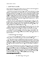
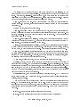
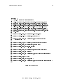
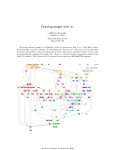
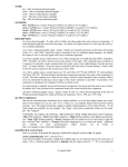
dot draws directed graphs as hierarchies. Like its predecessor, dag, it is a Unix lter,
makes good drawings, and runs quickly. Its important new features are node ports for
drawing data structures with pointers; improved placement of nodes, edge splines and labels;
cluster layouts; and an underlying le language for graph tools. Here is a reduced module
dependency graph of the SML-NJ compiler. The layout took 3.5 seconds of user time on
an HP-9000/730 computer.
IntSparcD
Batch
CompSparc
IntSparc
RealDebug
IntNull
IntNullD
BogusDebug
Stream
Join
LrTable
Backpatch
IntShare
Interact
UnixPaths
ModuleComp
PrimTypes
ProcessFile
Importer
LambdaOpt
Linkage
Translate
Coder
SparcAsCode
SparcCM
SparcInstr
BaseCoder
SparcMCEmit
SparcMC
SparcMCode
IEEEReal
Closure
RealConst
CPSgen
Bigint
CPSsize
ContMap
FreeMap
CPSopt
Spill
GlobalFix
Expand
Contract
CPSprint
CPS
Prof
Hoist
Reorder
Eta
Intset
Interp
Convert
Lambda
CoreInfo
Sort
PrintUtil
Absyn
Unboxed
MLLexFun
Variables
Siblings
Intmap
Access
EqTypes
Modules
TypesUtil
Fixity
BasicTypes
Types
Stamps
Symbol
StrgHash
Env
Index
Vector
Tuples
Unionfind
Unsafe
CoreFunc
InLine
Signs
SigMatch
Prim
Dynamic
Core
MLLrValsFun
InlineOps
Opt
SortedList
List2
Dummy
ApplyFunctor
MCprint
Equal
Math
Fastlib
Strs
ModuleUtil
ErrorMsg
LrParser
MCopt
ClosureCallee
PolyCont
FreeLvar
Nonrec
CPScomp
Profile
NewParse
JoinWithArg
MC
SparcAsEmit
Loader
Initial
CG
SparcAC
Overloads
PersStamps
IntStrMap
Pathnames
dot User's Manual, October 18, 1993
PrintAbsyn
BareAbsyn
PrintType
ArrayExt
PrintVal
PrintDec
Misc
Overload
AbstractFct
Unify
Ascii
TyvarSet
Typecheck
Instantiate
PrintBasics
Normalize
CoreLang
ConRep
Assembly
CInterface
MakeMos
CleanUp
Drawing graphs with dot
2
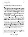
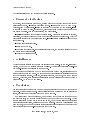
1 Basic Graph Drawing
dot draws directed graphs. It reads attributed graph text les and writes drawings, either
as graph les or in a graphics language such as PostScript.
dot takes four main steps in drawing a graph. Knowing about these helps you to understand what kind of layouts dot makes, and how you can modify its layouts. The rst
step assigns discrete ranks to nodes. In a top to bottom drawing, ranks determine Y coordinates. Edges that span more than one rank are broken into chains of \virtual" nodes and
unit-length edges. The second step orders nodes within ranks to avoid crossings. The third
step sets X coordinates of nodes to keep edges short. The last step routes edge splines.
This is the same general approach as dag, which in turn builds on the work of Wareld
[War77], Carpano [Car80] and Sugiyama [STT81]. We refer the reader to [GKNV93] for
explanation of dot's algorithms.
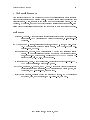
dot's graph language has three kinds of items: graphs, nodes, and edges. The main
(outermost) graph can be graph (undirected) or a digraph (directed). Because dot makes
layouts of directed graphs, all the examples in this user's guide use digraph. We have
written a separate layout utility, n eato, to draw undirected graphs [Nor92]. Within a main
graph, a subgraph denes a subset of nodes and edges.
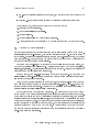
Figure 1 is an example graph in dot's language. Line 1 gives the graph name and type.
The following lines create nodes, edges, or subgraphs, and set attributes. Names may be C
identiers, numbers, or quoted C strings. Quotes protect punctuation or white space.
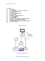
A node is created the rst time its name appears in the le. An edge is created when
nodes are joined by the edge operator ->. In the example, line 2 makes edges from main
to parse and from parse to execute. Running dot on this le (say graph1.dot) yields the
drawing of gure 2 1
$ dot -Tps graph1.dot -o graph1.ps
The command line option -Tps selects PostScript (EPSF) output. graph1.ps may be
printed, displayed by a PostScript viewer, or embedded in another document.
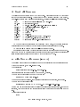
It is often useful to adjust the representation or placement of nodes and edges in the
layout. This is done by setting attributes of nodes, edges, or subgraphs in the input le.
Attributes are name-value pairs of character strings. Figures 3 and 4 illustrate some layout
attributes. In the listing of gure 3, line 2 sets the graph's size to 4,4 (all dimensions are
in inches). This attribute controls the bounding box{ the drawing is scaled as necessary to
t.
Node or edge attributes are set o in square brackets. In line 3, the node main is
assigned shape box. The edge in line 4 is straightened by increasing its weight (the default
is 1). The edge in line 6 is drawn as a dotted line. Line 8 makes edges from execute to
make string and printf. In line 10 the default edge color is set to red. This aects any
edges created after this point in the le. Line 11 makes a bold edge labeled 100 times. In
line 12, node make_string is given a multi-line label. Line 13 changes the default node to
be a box lled with a shade of blue. The node compare inherits these values.
1
Unlike dag, the .GS command is not needed.
dot User's Manual, October 18, 1993
Drawing graphs with dot
1: digraph G {
2:
main ->
3:
main ->
4:
main ->
5:
execute
6:
execute
7:
init ->
8:
main ->
9:
execute
10: }
3
parse -> execute;
init;
cleanup;
-> make_string;
-> printf
make_string;
printf;
-> compare;
Figure 1: Small graph
main
parse
init
cleanup
execute
make_string
compare
printf
Figure 2: Drawing of small graph
dot User's Manual, October 18, 1993
Drawing graphs with dot
4
1: digraph G {
2:
size ="4,4";
3:
main [shape=box];
/* this is a comment */
4:
main -> parse [weight=8];
5:
parse -> execute;
6:
main -> init [style=dotted];
7:
main -> cleanup;
8:
execute -> { make_string; printf}
9:
init -> make_string;
10:
edge [color=red];
11:
main -> printf [style=bold,label="100 times"];
12:
make_string [label="make a\nstring"];
13:
node [shape=box,style=filled,color=".7 .3 1.0"];
14:
execute -> compare;
15: }
Figure 3: Fancy graph
main
parse
init
cleanup
100 times
execute
make a
string
compare
printf
Figure 4: Drawing of fancy graph
dot User's Manual, October 18, 1993
Drawing graphs with dot
5
2 Drawing Attributes
The complete list of attributes that aect graph drawing is summarized in table 1.
2.1 Shapes and Labels
By default, nodes are drawn with shape=ellipse, width=.75, height=.5, and labeled by
the node name. Other common shapes (box, circle, etc.) are listed in table 1. The node
shape plaintext is of particularly interest in that it draws a node without any outline, an
important convention in some kinds of diagrams. When drawn, a node's actual size is the
greater of the requested size and the area needed for its text label. By default, edges are
unlabeled. Node and edge labels can be set explicitly as shown n gure 4. Though it is
convenient that nodes are labeled with their names by default, sometimes it is essential to
set labels explicitly. For example, in drawing a le directory tree, one might have several
directories named src, but each one must have a unique node identier. The inode number
or full path name are suitable unique identiers. Then the label of each node can be set to
the le name within its directory.
In multi-line labels, \n, \l, \r terminate lines that are centered, or left or right justied.2
Graphs and cluster subgraphs may also have labels.
The default font is 14-point Times-Roman, in black. Other font families, sizes, and colors
may be selected. Font names should be compatible with the target interpreter (usually
PostScript). It is best to use only the standard font families Times, Helvetica, Courier, or
Symbol as these are guaranteed to work with any target graphics language. For example,
Times-Italic, Times-Bold, or Courier are portable, but AvanteGarde-DemiOblique is
not.
Nodes with shape record or polygon have special properties. Section 3 reviews some
details of using records. Polygons are useful for many shapes that are not predened.
They are parameterized by number of sides, peripheries, orientation, skew, and distortion,
as illustrated in gures 5 and 6. peripheries is the number of borders. For example,
a doublecircle has 2 peripheries. orientation is clockwise rotation from the axis in
degrees. skew is a oating point number (usually between ,1 0 and 1 0) that distorts the
shape by slanting it from top-to-bottom, for example, turning a box into a parallelogram.
distortion shrinks from top-to-bottom, for example, turning a box into a trapezoid.
Though there is a way to implement custom node shapes, the details are beyond the
scope of this user's guide. Please contact the authors for further information.
X
:
:
2.2 Graphics Styles
Nodes and edges have color and style attributes. A color value can be a hue-saturationbrightness triple (three oating point numbers between 0 and 1), or one of the colors names
listed in Appendix B (borrowed from some version of the X window system). The numerical
2
The escape nN is an internal symbol for node names.
dot User's Manual, October 18, 1993
Drawing graphs with dot
Name
6
Default
color
fontcolor
fontname
fontsize
height width
label
shape
,
style
color
decorate
dir
fontcolor
fontname
fontsize
id
label
minlen
style
weight
center
clusterrank
color
concentrate
fontcolor
fontname
fontsize
label
margin
mclimit
nodesep
nslimit
ordering
orientation
page
rank
rankdir
ranksep
ratio
size
Values
Node Attributes
black
node shape color
black
type face color
Times-Roman PostScript font family
14
point size of label
.5,.75
height and width in inches
node name any string
ellipse
ellipse, box, circle, doublecircle, diamond,
plaintext, record, polygon
graphics options, e.g. bold, dotted, filled
Edge Attributes
black
edge stroke color
if set, draws a line connecting labels with their edges
forward
forward, back, both, or none
black
type face color
Times-Roman PostScript font family
14
point size of label
optional value to distinguish multiple edges
label, if not empty
1
minimum rank distance between head and tail
graphics options, e.g. bold, dotted, lled
1
integer reecting importance of edge.
Graph Attributes
when set, centers drawing on page
local
may be global or none
black
cluster box stroke color
enables edge concentrators when TRUE
black
type face color
Times-Roman PostScript font family
14
point size of label
any string
.5,.5
margin included in page
1.0
if set to f, adjusts mincross iterations by (f)
.25
separation between nodes, in inches.
if set to f, bounds network simplex iterations by
(f)(number of nodes)
out (for ordered edges)
portrait
may be set to landscape
unit of pagination, e.g. 8.5,11
same, min, or max
TB
LR (left to right) or TB (top to bottom)
.75
separation between ranks, in inches.
approximate aspect ratio desired, or fill
drawing bounding box, in inches
Table 1: Drawing attributes
dot User's Manual, October 18, 1993
Drawing graphs with dot
7
a
e
b
c
d
Figure 5: Example of polygonal shapes for nodes
1:
2:
3:
4:
5:
6:
7:
8:
digraph G {
a -> b -> c;
b -> d;
a [shape=polygon,sides=5,peripheries=3,color=blue_light,style=filled];
c [shape=polygon,sides=4,skew=.4,label="hello world"]
d [shape=invtriangle];
e [shape=polygon,sides=4,distortion=.7];
}
Figure 6: Listing of graph with polygonal shapes
dot User's Manual, October 18, 1993
Drawing graphs with dot
8
form is convenient for scripts or tools that automatically generate colors. Color name lookup
case and puncutation and insensitive, so "warmgrey" and Warm_Grey are equivalent.
We can oer a few hints regarding use of color in graph drawings. First, avoid using
too many bright colors. A \rainbow eect" is confusing. It's better to choose a narrower
range of colors, or to vary saturation along with hue. Second, when nodes are lled with
dark or very saturated colors, labels seem to be more readable with fontcolor=white and
fontname=Helvetica. (We also have PostScript functions for dot that create outline fonts
from plain fonts.) Third, you can dene your own color space by redening nodecolor,
edgecolor, or graphcolor in a library le. For example, to use RGB colors, place the
following line in a le lib.ps.
/nodecolor {setrgbcolor} bind def
Use the -l command line option to load this le.
dot -Tps -l lib.ps file.dot -o file.ps
style controls miscellaneous graphics features of nodes, edges, graphs or subgraphs.
The style is a list of primitives with optional argument lists. The predened primitives are
filled solid dashed dotted bold and invis. filled when applied to nodes or clusters
shades inside the boundary of the object using its color. If the color is not set, light grey
is used as the default.
User-dened style primitives can be implemented as custom PostScript procedures. Such
primitives are executed inside the gsave context of a graph, node, or edge, before any of its
marks are drawn. The arg lists are translated to PostScript notation. For example, a node
with style="setlinewidth(8)" is drawn with a thick outline. Here, setlinewidth is a
PostScript built-in, but user-dened PostScript procedures are called the same way. The
denition of these procedures can be given in a library le loaded using -l as shown above.
Edges have a dir attribute to set arrowheads. dir may be forward (the default), back,
both, or none. This refers only to where arrowheads are drawn, and does not change the
underlying graph. For example, setting dir=back does not exchange the endpoints of a
directed edge (unlike the dagprogram).
2.3 Drawing Size and Spacing
Often a drawing made with the default node sizes and separations is too big for the target
printer or for the space allowed for a gure in a document. There are several ways to try
to deal with this problem. First, we will review how dot computes the nal layout size.
A layout is initially made internally at its \natural" size, using default settings (unless
ratio=compress was set, as described below). By default, nodes are at least .75 (inches)
wide by .5 tall; fonts are 14 points high; nodes are separated by at least .25 and ranks by
.5. There is no bound on the size or aspect ratio of the drawing, so if the graph is large,
the layout is also large. If you don't specify size or ratio, then the natural size layout is
printed.
dot User's Manual, October 18, 1993
Drawing graphs with dot
9
The easiest way to control the output size of the drawing is to set size= in the
graph le (or on the command line using -G). This determines the bounding box of the nal
layout. For example, size="7.5,10" ts on an 8.5x11 page (assuming the default page
orientation) no matter how big the initial layout. ratio also aects layout size. There are
a number of cases, depending on the settings of size and ratio.
Case 1. ratio was not set. If the drawing already ts within the given size then
nothing happens. Otherwise, the drawing is reduced uniformly enough to make the critical
dimension t.
If ratio was set, there are four subcases.
Case 2a. If ratio= where
is a oating point number, then the drawing is stretched
(adding whitespace) to achieve the requested ratio expressed as drawing
. For
example, ratio=2.0 makes the drawing twice as wide as it is high. Then the layout is
scaled using size as in Case 1.
Case 2b. If ratio=fill and size=
was set, then the drawing is stretched (adding
whitespace) to achieve the ratio . The eect is that all of the bounding box given by
size is lled. Then scaling is performed as in Case 1.
Case 2c. If ratio=compress and size=
was set, then the initial layout is compressed
to attempt to t it t it the given bounding box. This trades o layout quality, balance,
and symmetry, to pack the layout more tightly. Then scaling is performed as in Case 1.
Case 2d. If ratio=auto then size is ignored and dot computes an \ideal" size using
the following heuristic: it rst attempts to t the drawing on one page by reducing to not
less than 50% of its original size. Otherwise, the drawing is printed on multiple pages, using
the full area of each page and not reducing under 50%.
At this point, if page is not set, then the nal layout is printed as one page.
If page= is set, then the layout is printed as a sequence of pages that can tiled or
assembled into a mosaic. Common settings are page="8.5,11" or page="11,17". These
values refers to the size of the physical device, and are independent of landscape mode. For
tiled layouts, you may nd it helpful to set smaller margins (the default is margin=.5).
Although you can set margin=0, unfortunately, many bitmap printers have an Internal
hardware margin that cannot be overridden.
If rotate=90 is set, then the layout is printed in landscape mode. The axis of the
layout would be along the axis of each page. This does not aect the dot's interpretation
of size, ratio, or "page.
A common problem is that a large graph drawn at a small size yields unreadable node
labels. To make larger labels, something has to give. There is a limit to the amount of
readable text that can t on one page. Often you can draw a smaller graph by extracting
an interesting piece of the original graph before running dot. We have some tools that help
with this.
x; y
x
x
width=height
x; y
x=y
x; y
x; y
X
Y
sccmap - decompose into strongly connected components
tred - compute transitive reduction (remove edges implied by transitivity)
dot User's Manual, October 18, 1993
Drawing graphs with dot
10
gpr - "raph processor to select nodes or edges, and contract or remove the rest of the
graph
unatten - improve aspect ratio of trees by staggering the lengths of leaf edges
With this in mind, here are some thing to try on a given graph:
1. Increase the node fontsize.
2. Use smaller ranksep and nodesep.
3. Use ratio=auto.
4. Use ratio=compress and give a reasonable size.
5. A sans serif font (such as Helvetica) may be more readable than Times when reduced.
2.4 Node and Edge Placement
Sometimes it is natural to make edges point from left to right instead of from top to bottom.
If rankdir=LR in the top-level graph, the drawing is rotated in this way. TB (top to bottom)
is the default. (BT seems potentially useful for drawing upward-directed graphs, but hasn't
been impelemented. In some graphs you could achieve the same eect by reversing the
endpoints of edges and setting their dir=back.)
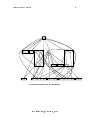
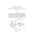
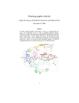
In graphs with time-lines, or in drawings that emphasize source and sink nodes, you
may need to constrain rank assignments. The set of a subgraph may be set to minrank,
maxrank, or samerank. This constrains the nodes in the subgraph. Figures 7 and 8 illustrate
using subgraphs for controlling rank assignment.
In some graphs, the left-to-right ordering of nodes is important. If a subgraph has
ordering=out then out-edges within the subgraph having the same tail node fan out from
left to right in their order of creation.
Also, when nodes are constrained to the same rank, edges with non-zero weight between
them are aimed across the rank in the same direction (left-to-right, or top-to-bottom in a
rotated drawing) as far as possible. This fact may be exploited to adjust node ordering by
placing invisible edges (style="invis") where needed.
Fine tuning should be approached cautiously. dot works best when it can makes a
layout without much \help" or interference in its placement of individual nodes and edges.
Layouts can be adjusted somewhat by increasing the weight\ of certain edges, or by creating
invisible edges or nodes using style=invis, and sometimes even by rearranging the order
of nodes and edges in the le. But this can backre because the layouts are not necessarily
stable with respect to changes in the input graph. One last adjustment can invalidate all
previous changes and make a very bad drawing. A future project we have in mind is to
combine the mathematical layout techniques of dot with an interactive front end that allows
user-dened hints and constraints.
dot User's Manual, October 18, 1993
Drawing graphs with dot
11
digraph asde91 {
ranksep=.75;
size = "7.5,7.5";
{
node [shape=plaintext, fontsize=16];
/* the time-line graph */
past -> 1978 -> 1980 -> 1982 -> 1983 -> 1985 -> 1986 ->
1987 -> 1988 -> 1989 -> 1990 -> "future";
/* ancestor programs */
"Bourne sh"; "make"; "SCCS"; "yacc"; "cron"; "Reiser cpp";
"Cshell"; "emacs"; "build"; "vi"; "<curses>"; "RCS"; "C*";
}
{ rank = same;
"Software IS"; "Configuration Mgt"; "Architecture & Libraries";
"Process";
};
node [shape=box];
{
{
{
{
{
{
{
{
{
{
{
{
rank = same; "past"; "SCCS"; "make"; "Bourne sh"; "yacc"; "cron"; }
rank = same; 1978; "Reiser cpp"; "Cshell"; }
rank = same; 1980; "build"; "emacs"; "vi"; }
rank = same; 1982; "RCS"; "<curses>"; "IMX"; "SYNED"; }
rank = same; 1983; "ksh"; "IFS"; "TTU"; }
rank = same; 1985; "nmake"; "Peggy"; }
rank = same; 1986; "C*"; "ncpp"; "ksh-i"; "<curses-i>"; "PG2"; }
rank = same; 1987; "Ansi cpp"; "nmake 2.0"; "3D File System"; "fdelta";
"DAG"; "CSAS";}
rank = same; 1988; "CIA"; "SBCS"; "ksh-88"; "PEGASUS/PML"; "PAX";
"backtalk"; }
rank = same; 1989; "CIA++"; "APP"; "SHIP"; "DataShare"; "ryacc";
"Mosaic"; }
rank = same; 1990; "libft"; "CoShell"; "DIA"; "IFS-i"; "kyacc"; "sfio";
"yeast"; "ML-X"; "DOT"; }
rank = same; "future"; "Adv. Software Technology"; }
"PEGASUS/PML" -> "ML-X";
"SCCS" -> "nmake";
"SCCS" -> "3D File System";
"SCCS" -> "RCS";
"make" -> "nmake";
"make" -> "build";
"Bourne sh" -> "Cshell";
"Bourne sh" -> "ksh";
"Reiser cpp" -> "ncpp";
"Cshell" -> "ksh";
.
.
.
}
Figure 7: Graph with constrained ranks
dot User's Manual, October 18, 1993
Drawing graphs with dot
12
past
SCCS
1978
make
Bourne sh
build
1980
RCS
vi
C*
DAG
3D File System
CIA
SBCS
APP
DOT
DIA
Ansi cpp
CIA++
<curses-i>
fdelta
TTU
ksh-i
PG2
nmake 2.0
PAX
ksh-88
PEGASUS/PML
SHIP
libft
Software IS
IMX
Peggy
ncpp
CSAS
1989
future
IFS
nmake
1988
1990
SYNED
ksh
1985
1987
emacs
<curses>
1983
1986
cron
Cshell
Reiser cpp
1982
yacc
backtalk
ryacc
CoShell
sfio
Configuration Mgt
IFS-i
ML-X
Architecture & Libraries
Adv. Software Technology
Figure 8: Drawing with constrained ranks
dot User's Manual, October 18, 1993
DataShare
Mosaic
kyacc
yeast
Process
Drawing graphs with dot
1:
2:
3:
4:
5:
6:
7:
8:
9:
10:
11:
12:
13:
14:
15:
16:
17:
18:
19:
20:
digraph g {
node [shape =
node0[label =
node1[label =
node2[label =
node3[label =
node4[label =
node5[label =
node6[label =
node7[label =
node8[label =
"node0":f2 ->
"node0":f0 ->
"node1":f0 ->
"node1":f2 ->
"node2":f2 ->
"node2":f0 ->
"node4":f2 ->
"node4":f0 ->
}
13
record,height=.1];
"<f0> |<f1> G|<f2>
"<f0> |<f1> E|<f2>
"<f0> |<f1> B|<f2>
"<f0> |<f1> F|<f2>
"<f0> |<f1> R|<f2>
"<f0> |<f1> H|<f2>
"<f0> |<f1> Y|<f2>
"<f0> |<f1> A|<f2>
"<f0> |<f1> C|<f2>
"node4":f1;
"node1":f1;
"node2":f1;
"node3":f1;
"node8":f1;
"node7":f1;
"node6":f1;
"node5":f1;
"];
"];
"];
"];
"];
"];
"];
"];
"];
Figure 9: Binary search tree using records
3 Node Ports
A node port is a point where edges may attach to a node. (When an edge is not attached
to a port, it is aimed at the node's center.) A node with a port specier has the syntax
name:port. The names and bindings of ports can dier from one node to another, depending
on shapes and other attributes. Presently only the record shape has ports. This shape
represents a record as recursive lists of labeled boxes. A port refers to the center of one of
the boxes. Ports are created by inserting the construct <portid> in a box label, as shown in
gures 9 and 10.
Figures 11 and 12 shows how recursive records are drawn. Vertical bars separate elds
at the same level, while curly braces enclose subeld lists. Port identiers are enclosed
in angle brackets. (Literal braces, vertical bars, and angle brackets must be escaped.)
Spaces are interpreted as separators between tokens (similar to the way most typesetting
programs work) so they must be escaped if you want xed or \hard" spaces. Also, note
that records sometimes look better if their input height is set to a small value so the text
labels dominate the actual size, as illustrated in gure 9. Otherwise the default node size
( 75 by 5) is assumed, as in gure 11.
The example of gures 13 and 14 uses left-to-right drawing in a layout of a hash table.
:
:
dot User's Manual, October 18, 1993
Drawing graphs with dot
14
G
E
B
R
F
A
H
Y
C
Figure 10: Drawing of binary search tree
1:
2:
3:
4:
5:
6:
7:
8:
digraph structs {
node [shape=record];
struct1 [shape=record,label="<f0> left|<f1> middle|<f2> right"];
struct2 [shape=record,label="<f0> one|<f1> two"];
struct3 [shape=record,label="hello\nworld |{ b |{c|<here> d|e}| f}| g | h"];
struct1:f1 -> struct2:f0;
struct1:f2 -> struct3:here;
}
Figure 11: Records with nested elds
left
middle
one two
right
hello
world
b
c d
f
e g
Figure 12: Drawing of records
dot User's Manual, October 18, 1993
h
Drawing graphs with dot
1:
2:
3:
4:
5:
6:
7:
8:
9:
10:
11:
12:
13:
14:
15:
16:
17:
18:
19:
20:
21:
22:
23:
15
digraph G {
nodesep=.05;
rankdir=LR;
node [shape=record,width=.1,height=.1];
node0 [label = "<f0>
node [width = 1.5];
node1 [label = "{<n>
node2 [label = "{<n>
node3 [label = "{<n>
node4 [label = "{<n>
node5 [label = "{<n>
node6 [label = "{<n>
node7 [label = "{<n>
|<f1> |<f2> |<f3> |<f4> |<f5> |<f6> | ",height=2.5];
n14
a1
i9
e5
t20
o15
s19
|
|
|
|
|
|
|
719
805
718
989
959
794
659
|<p>
|<p>
|<p>
|<p>
|<p>
|<p>
|<p>
}"];
}"];
}"];
}"];
}"] ;
}"] ;
}"] ;
node0:f0 -> node1:n;
node0:f1 -> node2:n;
node0:f2 -> node3:n;
node0:f5 -> node4:n;
node0:f6 -> node5:n;
node2:p -> node6:n;
node4:p -> node7:n;
}
Figure 13: Hash table graph le
n14
719
a1
805
i9
718
e5
989
t20
959
o15
794
s19
659
Figure 14: Drawing of hash table
dot User's Manual, October 18, 1993
Drawing graphs with dot
16
digraph G {
subgraph cluster0 {
node [style=filled,color=white];
style=filled;
color=lightgrey;
process
a0 -> a1 -> a2 -> a3;
label = "process #1";
b0
}
subgraph cluster1 {
node [style=filled];
b0 -> b1 -> b2 -> b3;
label = "process #2";
color=blue
}
start -> a0;
start -> b0;
a1 -> b3;
b2 -> a3;
a3 -> a0;
a3 -> end;
b3 -> end;
start
#2
process #1
a0
b1
a1
b2
a2
b3
a3
start [shape=Mdiamond];
end [shape=Msquare];
}
end
Figure 15: Process diagram with clusters
3.1 Clusters
A cluster is a subgraph placed in its own distinct rectangle of the layout. A subgraph is recognized as a cluster when its name has the prex cluster (unless the graph's clusterrank=none).
Cluster labels, fonts, colors, and styles can be set in the usual way. Clusters are drawn by a
recursive technique that computes a rank assignment and internal ordering of nodes within
clusters. Figure 15 through 17 are cluster layouts and the corresponding graph les.
3.2 Concentrators
Setting concentrate=true on the top level graph enables an edge merging technique to
reduce clutter in dense layouts. Edges are merged when they run parallel and have a
common endpoint. A benecial side-eect in xed-sized layouts is that removal of these
edges often permits larger, more readable labels. While dot's concentrators look somewhat
like Newbery's [New89], they are found by searching the edges in the layout, not by detecting
complete bipartite graphs in the underlying graph. Thus the dot approach runs much faster
dot User's Manual, October 18, 1993
Drawing graphs with dot
17
main
util.c
init_index
getopt
ciafan.c
debug
stringdup
fan
ciafan
error.h
fatal
sfio.h
sfprintf
exit
query.h
interp_err
stdlib.h
stdio.h
malloc
free
realloc
stdsprintf
increment
ref
def
computefan
string.h
stdprintf
strcpy
Figure 16: Call graph with labeled clusters
dot User's Manual, October 18, 1993
strcat
strlen
strcmp
get_sym_fields
Drawing graphs with dot
18
1:digraph G {
2: size="8,6"; ratio=fill; node[fontsize=24];
3:
4: ciafan->computefan; fan->increment; computefan->fan; stringdup->fatal;
5: main->exit; main->interp_err; main->ciafan; main->fatal; main->malloc;
6: main->strcpy; main->getopt; main->init_index; main->strlen; fan->fatal;
7: fan->ref; fan->interp_err; ciafan->def; fan->free; computefan->stdprintf;
8: computefan->get_sym_fields; fan->exit; fan->malloc; increment->strcmp;
9: computefan->malloc; fan->stdsprintf; fan->strlen; computefan->strcmp;
10: computefan->realloc; computefan->strlen; debug->sfprintf; debug->strcat;
11: stringdup->malloc; fatal->sfprintf; stringdup->strcpy; stringdup->strlen;
12: fatal->exit;
13:
14: subgraph "cluster_error.h" { label="error.h"; interp_err; }
15:
16: subgraph "cluster_sfio.h" { label="sfio.h"; sfprintf; }
17:
18: subgraph "cluster_ciafan.c" { label="ciafan.c"; ciafan; computefan;
19:
increment; }
20:
21: subgraph "cluster_util.c" { label="util.c"; stringdup; fatal; debug; }
22:
23: subgraph "cluster_query.h" { label="query.h"; ref; def; }
24:
25: subgraph "cluster_field.h" { get_sym_fields; }
26:
27: subgraph "cluster_stdio.h" { label="stdio.h"; stdprintf; stdsprintf; }
28:
29: subgraph "cluster_<libc.a>" { getopt; }
30:
31: subgraph "cluster_stdlib.h" { label="stdlib.h"; exit; malloc; free; realloc; }
32:
33: subgraph "cluster_main.c" { main; }
34:
35: subgraph "cluster_index.h" { init_index; }
36:
37: subgraph "cluster_string.h" { label="string.h"; strcpy; strlen; strcmp; strcat; }
38:}
Figure 17: Call graph le
dot User's Manual, October 18, 1993
Drawing graphs with dot
19
but doesn't collapse as many edges as Newbery's algorithm.
4 Command Line Options
By default, dot operates in lter mode, writing graphs in the input format with layout
attributes appended. -Tps sets PostScript output. -Tpcl emits HPGL/2 with PCL-5
wrappers, for HP Laserwriters. -Thpgl emits pure HPGL for wide bed pen plotters. -Tmif
emits FrameMaker MIF les. In this mode, graph layouts can be loaded into FrameMaker
and edited manually. FrameMaker is limited to 8 basic colors.
-Gname=value sets a graph attribute default value. Often it is convenient to set size,
pagination, and related values on the command line rather than in the graph le. Note that
le contents override command line arguments. -N or -E instead of -G set default node or
edge attributes.
-l loads graphics library les.
-o sets the output le.
-v requests verbose output. In processing large layouts, the verbose messages may give
some estimate of dot's progress.
-V prints the version number.
5 Miscellaneous
There are several features of the graph le language worth noting. In the top-level graph
heading, a graph may be declared a strict digraph. This forbids the creation of self-arcs
and multi-edges; they are ignored in the input le.
If a subgraph appears with a body more than once in a graph le, its contents are the
union of all the nodes and edges. An edge id is an optional string for referencing an edge
that was previously created. When set, the triple (tail node, head node, key) form a unique
edge key. Otherwise, a new internal id is generated for each distinct edge between the same
pair of nodes. An id may be any string.
6 Conclusions
dot produces nicer drawings than dag and has some features to help make more readable
drawings. It is not as fast as dag. Since it still takes only a second or two on reasonable
inputs, we feel the new features more than make up for this.
In writing graph drawing programs, we have found that it does not take long to get
the rst drawings, but it takes a great deal of work to get truly good drawings. While
there is still plenty of room for improvement in dot, we have accomplished our principal
goals concerning aesthetics, performance and new features. Since the basic algorithms of
dot work well, we have a good basis for further research into problems such as methods for
drawing large graphs and on-line (animated) graph drawing.
dot User's Manual, October 18, 1993
Drawing graphs with dot
20
7 Acknowledgements
We would like to thank Emden Gansner and Phong Vo for discussions and advice regarding
graph drawing algorithms and program design. The graph library uses Phong's splay tree
dictionary library. Also, the users of dag shared many good suggestions with us. Emden
Gansner, Guy Jacobson, and Randy Hackbarth reviewed earlier drafts of this manual. John
Ellson wrote the generalized polygon shape and took pains to make it robust and ecient.
References
[Car80] M. Carpano. Automatic display of hierarchized graphs for computer aided decision analysis. IEEE Transactions on Software Engineering, SE-12(4):538{546,
April 1980.
[GKNV93] Emden R. Gansner, Eleftherios Koutsoos, Stephen C. North, and Kiem-Phong
Vo. A Technique for Drawing Directed Graphs. IEEE Trans. Sofware Eng.,
19(3):214{230, May 1993.
[New89] Frances J. Newbery. Edge Concentration: A Method for Clustering Directed
Graphs. In 2nd International Workshop on Software Conguration Management, pages 76{85, October 1989. Published as ACM SIGSOFT Software Engineering Notes, vol. 17, no. 7, November 1989.
[Nor92] Stephen C. North. Neato User's Guide. Technical Report 59113-921014-14TM,
AT&T Bell Laboratories, Murray Hill, NJ, 1992.
[STT81] K. Sugiyama, S. Tagawa, and M. Toda. Methods for Visual Understanding
of Hierarchical System Structures. IEEE Transactions on Systems, Man, and
Cybernetics, SMC-11(2):109{125, February 1981.
[War77] John Wareld. Crossing Theory and Hierarchy Mapping. IEEE Transactions
on Systems, Man, and Cybernetics, SMC-7(7):505{523, July 1977.
dot User's Manual, October 18, 1993
Drawing graphs with dot
21
A Graph File Grammar
The following is an abstract grammar of graph les. Terminals are shown in typewriter
font and nonterminals in italics. Angle brackets h and i indicate grouping when needed.
Double-line brackets [ and ] enclose optional items. Vertical bars j separate alternatives.
graph
! [strict] h digraph j graph iid { stmt-list }
stmt-list ! [stmt [;] [stmt-list ] ]
stmt
! attr-stmt j node-stmt j edge-stmt j subgraph j id = id
attr-stmt ! hgraph j node j edgei[ [ attr-list ] ]
attr-list
! id=id [attr-list ]
node-stmt ! node-id [ opt-attrs ]
node-id
! id [: id ]
opt-attrs ! [attr-list]
edge-stmt ! hnode-id j subgraphi edgeRHS [opt-attrs ]
edgeRHS ! edgeop hnode-id j subgraphi [edgeRHS ]
subgraph ! [subgraph id] { stmt-list } j subgraph id
An id is any alphanumeric string not beginning with a digit, but possibly including
underscores; or a number; or any quoted string possibly containing escaped quotes.
An edgeop is -> in directed graphs and -- in undirected graphs.
Semicolons aid readability but are not required except in the rare case that a named subgraph with no body immediate preceeds an anonymous subgraph, because under precedence
rules this sequence is parsed as a subgraph with a heading and a body.
B Plain Output File Format (-Tplain)
The \plain" output format of dot lists node and edge coordinates that are usually needed
by front end programs, in a line-oriented style.
The rst line is:
graph scalefactor bounding box x bounding box y
All coordinates are in default units (1/72 of an inch), unscaled.
The next group of lines list the nodes in the format:
node name x y xsize ysize label text
The name is a unique identier. If it contains whitespace or punctuation, it is quoted.
The next group of lines list edges:
edge tailname headname
1 1 2 2
n n opt text opt x opt y
is the number of coordinate pairs that follow as Bezier spline control points. If the edge
is labeled, then the label text and coordinates are listed as the rightmost three items on the
line.
The last line is always:
n x
y
x
y
::: x
y
n
stop
dot User's Manual, October 18, 1993
Drawing graphs with dot
22
C Layout Attributes
Layout coordinates are in the default PostScript coordinate system. Node coordinates refer
to their center points. The edge spline is a list of 3 +1 points, plus optional s and optional
e points.
The 3 + 1 points are the Bezier control points. Points 0 1 2 3 3 are the rst bezier
spline, 3 4 5 6 are the second, etc.
The s point is present if there's an arrow at 0 . In this case the arrow is from 0 to
point s , where s is actually on the node's boundary and 0 is further away. If there is no
arrow, 0 is on the node's boundary. Similarly, e is for an arrow on the other endpoint of
the edge.
Currently, edge points are listed top-to-bottom (or left-to-right) regardless of the orientation of the edge. This may change.
n
p
p
n
p ;p ;p ;p
p ;p ;p ;p
p
p
p
p
p
p
p
p
dot User's Manual, October 18, 1993
Drawing graphs with dot
23
D Color Names
Whites
antiquewhite[1-4]
azure[1-4]
bisque[1-4]
blanchedalmond
cornsilk[1-4]
oralwhite
gainsboro
ghostwhite
honeydew[1-4]
ivory[1-4]
lavender
lavenderblush[1-4]
lemonchion[1-4]
linen
mintcream
mistyrose[1-4]
moccasin
navajowhite[1-4]
oldlace
papayawhip
peachpu[1-4]
seashell[1-4]
snow[1-4]
thistle[1-4]
wheat[1-4]
white
whitesmoke
Greys
darkslategray[1-4]
dimgray
gray
gray[0-100]
lightgray
lightslategray
slategray[1-4]
Blacks
black
Reds
coral[1-4]
crimson
darksalmon
deeppink[1-4]
rebrick[1-4]
hotpink[1-4]
indianred[1-4]
lightpink[1-4]
lightsalmon[1-4]
maroon[1-4]
mediumvioletred
orangered[1-4]
palevioletred[1-4]
pink[1-4]
red[1-4]
salmon[1-4]
tomato[1-4]
violetred[1-4]
Browns
beige
brown[1-4]
burlywood[1-4]
chocolate[1-4]
darkkhaki
khaki[1-4]
peru
rosybrown[1-4]
saddlebrown
sandybrown
sienna[1-4]
tan[1-4]
Oranges
darkorange[1-4]
orange[1-4]
orangered[1-4]
Yellows
darkgoldenrod[1-4]
gold[1-4]
goldenrod[1-4]
greenyellow
lightgoldenrod[1-4]
lightgoldenrodyellow
lightyellow[1-4]
palegoldenrod
yellow[1-4]
yellowgreen
Greens
chartreuse[1-4]
darkgreen
darkolivegreen[1-4]
darkseagreen[1-4]
forestgreen
green[1-4]
greenyellow
lawngreen
lightseagreen
limegreen
mediumseagreen
mediumspringgreen
mintcream
olivedrab[1-4]
palegreen[1-4]
seagreen[1-4]
springgreen[1-4]
yellowgreen
Cyans
aquamarine[1-4]
cyan[1-4]
darkturquoise
lightcyan[1-4]
mediumaquamarine
mediumturquoise
paleturquoise[1-4]
dot User's Manual, October 18, 1993
turquoise[1-4]
Blues
aliceblue
blue[1-4]
blueviolet
cadetblue[1-4]
cornowerblue
darkslateblue
deepskyblue[1-4]
dodgerblue[1-4]
indigo
lightblue[1-4]
lightskyblue[1-4]
lightslateblue[1-4]
mediumblue
mediumslateblue
midnightblue
navy
navyblue
powderblue
royalblue[1-4]
skyblue[1-4]
slateblue[1-4]
steelblue[1-4]
Magentas
blueviolet
darkorchid[1-4]
darkviolet
magenta[1-4]
mediumorchid[1-4]
mediumpurple[1-4]
mediumvioletred
orchid[1-4]
palevioletred[1-4]
plum[1-4]
purple[1-4]
violet
violetred[1-4]