1
Science Payloads and Advanced Concepts for
Exploration (SPACE) Interactive Tool
Huong Vo, Zoe Himwich, Aparna Natarajan
Mentor: Dr. Pamela E. Clark
NASA Goddard Space Flight Center, Greenbelt, Maryland
Contents
1 INTRODUCTION
2
2 SUBSYTEMS
2.1 Mission Planning . . . . . . . . . . . . .
2.2 Instrument Selection . . . . . . . . . . .
2.3 Attitude Control System Selection . . . .
2.4 Propulsion Selection . . . . . . . . . . .
2.5 Communication Selection . . . . . . . . .
2.6 Command and Data Handling Selection .
2.7 Power Selection . . . . . . . . . . . . . .
2.8 Frame Selection . . . . . . . . . . . . . .
2.9 Final Result Page . . . . . . . . . . . . .
2.10 Inputs/Output Summary . . . . . . . . .
.
.
.
.
.
.
.
.
.
.
2
3
3
7
8
11
13
15
16
17
18
3 IMPLEMENTATION
3.1 Resolving Bugs . . . . . . . . . . . . . . . . . . . . . . . . . . . . . . . . . .
3.2 Obtaining a Copy of the Code . . . . . . . . . . . . . . . . . . . . . . . . . .
19
19
20
4 DATABASE
20
5 NEXT STEPS
20
6 REFERENCES
21
7 CONTACT US
21
1
.
.
.
.
.
.
.
.
.
.
.
.
.
.
.
.
.
.
.
.
.
.
.
.
.
.
.
.
.
.
.
.
.
.
.
.
.
.
.
.
.
.
.
.
.
.
.
.
.
.
.
.
.
.
.
.
.
.
.
.
.
.
.
.
.
.
.
.
.
.
.
.
.
.
.
.
.
.
.
.
.
.
.
.
.
.
.
.
.
.
.
.
.
.
.
.
.
.
.
.
.
.
.
.
.
.
.
.
.
.
.
.
.
.
.
.
.
.
.
.
.
.
.
.
.
.
.
.
.
.
.
.
.
.
.
.
.
.
.
.
.
.
.
.
.
.
.
.
.
.
.
.
.
.
.
.
.
.
.
.
.
.
.
.
.
.
.
.
.
.
.
.
.
.
.
.
.
.
.
.
.
.
.
.
.
.
.
.
.
.
2 SUBSYTEMS
Abstract
Here at Goddard Space Flight Center, we have developed an online CubeSat design
tool, geared towards deep space exploration based on a specific mission requirement –
henceforth referred to as the SPACE tool. The tool is ideal for scientists and engineers
who wants to draw up a complete, but preliminary system, consisting of parts that are a
mixture of commercial off the shelf, as well as research innovations – making the overall
cost much more manageable. SPACE walks the user through a series of questions and
forms, eventually parsing these parts together for a final design consisting of seven
separate subsystems. We hope that with the development of this tool, we can eventually
move towards a standardization of the CubeSat paradigm, making it cheaper, faster,
and easier than ever to design a CubeSat.
1
INTRODUCTION
CubeSats are small satellites grouped under the umbrella category of nano-satellites, coming
in units that are each 10 cm x 10 cm x 10 cm, weighing about 1.33 kg [1]. A CubeSat
can, and often, consists of multiple units of various configurations depending on the mission
requirements. It was first introduced in 1999, by Bob Twigs (Stanford) and Jordi Purig-Surai
(Cal Poly), in order to allow graduate students to develop and test small, low cost spacecraft
in low earth orbit [2]. Since then, the idea of miniature, economical spacecraft has become
increasingly popular, propagating CubeSat development as well as the miniaturization of
existing technologies all throughout the professional market.
While CubeSats have become very ubiquitous and economically sustainable within lowearth orbit, they are not being utilized to their full potentials – i.e., beyond the low-earth
orbit. We feel that this is the logical next step, based on several different facets of the
CubeSat paradigm. First and foremost, if we begin to use CubeSats for deep space science
missions, we can obtain a dynamic view of the target through a multi-platform approach,
instead of the current, static view we are able to achieve through the use of one conventional
spacecraft. Furthermore, CubeSats can be easily integrated as a secondary payload, with
minimal expenditures. Its small form factor allows for a reduction of launch costs, and the
standardization leads to a predictability that will reduce failure rates. With the SPACE Tool,
we are encouraging the user to develop missions for targets much beyond LEO (although that
will be an option), through introducing instrumentation and subsystems that were developed
for use in a deep space environment.
2
SUBSYTEMS
The tool consists of a series of webpages, beginning with the instrumentation and ending with
the thermal and mechanical subsystems. While SPACE can be used without a preconceived
mission requirement, it is better to come in to the design process with some preliminary
planning. This starts with the introduction page, which asks for a target planet that the
user would like to fly by. Choosing this target will affect the calculations later on during the
2
2.1 Mission Planning
2 SUBSYTEMS
trajectory planning, as well as the communication path. Knowing the science requirement
of the mission before starting this tool will also streamline the instrumentation selection
process, the most crucial selection of the entire design process – as the instrumentation is
the core of every science-based CubeSat.
That said, we have ensured to create a thoroughly documented website, so any new user
will be able to come in and create a CubeSat using the technologies we have laid out for
them. There are instructions and explanations on every page for the required inputs as well
as some suggested range that have been used in the past, and before the user even start the
tool, the landing page has a brief explanation of the algorithms we use to present the parts
on each page. Every subsection uses the same method to add a part to the current design,
which is responsive and straightforward, and the user will be able to go back and redesign
as they wish. However, only when a page is completely filled out, can a user move forward
– this ensures no bugs are created in later calculations. The user will also be able to see
a snapshot for their most up-to-date design on every page, as they are working. There is
also an icon, with the letter i in it for each page next to the available parts window, which
will let the user view more information about their desired part so they can make the choice
best suited for their mission. We will now proceed to describe each subpage in details, and
present our methods of filtering down available parts.
2.1
Mission Planning
In this section, the user is asked to fill out some brief descriptors of their mission – such as a
name, an objective, as well as their target planet. The objective can be as brief or as detailed
as the user wishes, and same goes for the name. The available targets for exploration are as
follow: Earth (in low, medium, or high orbit), Mercury, Mars, Venus, and the Moon. There
is a right arrow button next to each required fields, which the user can double click to add
the inputs to the current design. The user will be able to progress to the next page, when
all three fields are filled out and added to the CubeSat. One caveat: if the user chooses to
go to the previous page, their CubeSat will be removed from the database and they will lose
all their work.
2.2
Instrument Selection
In this section, the user is asked to choose an instrumentation for their CubeSat. This section
is crucial in the design process, as the instrumentation is what will carry out the science
requirements. The selection is revolved around the electromagnetic spectrum – based on the
guiding principle that each part of the spectrum is governed by different energy production
mechanisms, detection methods, as well as analysis technique associated. We have divided
the spectrum into five separate sub-region, with detailed explanations of what each section
can handle in terms of remote sensing. The general idea is that as the wavelengths increase,
the scale of the natural processes occurring that can be looked at with the light increases, but
so does the depth of penetration. It is recommended that the user at least knows the scale of
their science requirements, as it will help the user choose the right part of the spectrum, and
3
2.2 Instrument Selection
2 SUBSYTEMS
Figure 1: Screenshot of the mission planning page
have an appropriate set of instrumentation populate the window. Another caveat we have
for the user is that there detectors mixed in with various kinds of instruments, which do not
have a support system included with the part, so if the user were to choose a detector, they
need to allocate more mass, power, and volume for these support systems. We will proceed
to include an explanation of each part of the spectrum here.
1. Ray Region: this is the highest energy region, consisting of gamma-rays, X-rays, and
ultraviolet. The energies reflected from this surface in this region can result from the
interaction of high energy solar rays or cosmic solar rays. The energy spectra associated
is produced from properties intrinsic to the individial atoms that are being observed,
which can provide direct information on elemental abundance. Gamma rays and Xrays are completely absorbed by a body’s atmosphere – never reaching the surface of
planets, which makes it more suitable for studying atmosphereless bodies.
2. Circumvisible Region: this region consists of visible, near IR (NIR), and short IR (SIR).
The source can come from natural light, artifical light, or lasers. The energy spectra
associated can be produced by transition in energy states of an individual atom’s
outermost electrons from the absorption of light – this occurs for elements in the alkali,
alkali earth, and transition metals group. Thus, instruments measuring visible/NIR
reflectance can obtain the relative abundance of those minerals. By observing the
albedo of said minerals, we can also obtain information about the reflectivity, as well
as the age of the deposit.
4
2.2 Instrument Selection
2 SUBSYTEMS
3. Infrared Region: this region consists of mid to far IR (MIR and FIR). The energy
spectra associated can be produced naturally from the absorption and transmittance
of ambient solar infrared energy, or induced by an active source (laser) leading to
interactions between and amongst atoms on the molecular level. Due to the scale of
natural processes occuring within this region, we are also able to look at fundamental
molecular vibrations associated with minerals, as well as water and hydroxyl. The
infrared signatures can also be used to distinguish between chemical groups, structural
groups, and polymorphs.
4. Longwave Region: this region consists of thermal, microwave, and radio. The source
can come from natural background radiation, emission from target, or from transmitters. The energy spectra associated can be produced by acceleration of free electrons
due to inelastic collisions, as well as variations in EM fields of molecules. Due to the
longer wavelength, and lower energies produced, we are able to observe much larger
scale processes in various phases. In the atmosphere, by observing a characteristic
frequency, we can determine the composition and density of the medium. In a liquid
body, we can record its salinity, and wave strength. In a solid body, we can look at a
surface roughness, as well as variation in moisture content. If a thermal measurement
is included, the particle size distribution of a surface can also be characterized.
5. Acoustic Region: this is the lowest energy region, consisting of sound, and seismic
waves. The signals in this region can be generated passively by electromagnetic or
gravitational field interactions, or actively by low frequency waves. To measure gravitational interaction between bodies, we can track the variation in calculated vs. actual
motion of a spacecraft with a radio transmitter. We can also use acoustic instruments
to interact with a surrounding material, and look at the underlying composition of a
celestial body.
Within each region of the EM spectrum (from ray to longwave), we continued to divide up
the wavelengths into more specific categories [3]:
1. Gamma rays: looking at this sub-region will let you observe radioactive elements with
natural decay lines such as potassium, thorium, or uranium.
2. X-rays: looking at this sub-region will let you observe elements with characteristic
fluorescent X-ray lines such as magnesium, aluminum, silicon, calcium, sulfur, titanium,
or iron.
3. UV: historically, UV wavelengths have been used to study ozone, sulfur dioxide, and
trace gases, in addition to airglow, auroral atmosphere and ionizating radiation.
4. Cosmic rays: can generate a cascade of small particles (including neutrons), which can
interact with nuclei of elements with large cross-sections (such as iron, titanium, and
rare earth elements), generating characteristic secondary gamma-ray lines.
5
2.2 Instrument Selection
2 SUBSYTEMS
5. Visible light: looking at this sub-region (which is the only region of light that can be
seen with the naked eye) can tell you many things, including flora/fauna identification,
rock and soil mineralogy, color, texture, photogeology, and photobotany.
6. Near/Short infrared: these spectral reflectance are widely used for diagnostic of rock
type in exposed planetary regoliths. Spectral absorption features are also used to look
at iron, other cations in silicate crystal lattices, as well as hydroxyl and carbonate, and
simple molecules in gaseous state adsorbed or loosely bonded to silicates such as CO2,
CO, H2O, and other small H, C, O bearing molecules.
7. Mid infrared: looking at this sub-region will let you see characteristic ’fingerprints’
associated with larger, more complex minerals, silicate, and non-silicate.
8. Long/Far infrared: looking at this sub-region, especially for very long wavelengths
associated with heat transporting properties will let you see the particular size, density,
and thermal conductivity of the surface.
9. Radiowave: looking at this subregion will let you look at the surface roughness at
interfaces, on scales from millimeters to meters. Because of the longer wavelengths,
you can also determine the speed/direction of objects, as well as the atmosphere and
weather condition.
10. Microwave: looking at this subregion will tell you the reflection and absorption of
liquids or solids associated with dielectric properties, particulary at interfaces between
fases, liquids, and solids.
We will also go over the type of instrumentation we have available, and the part of the
electromagnetic spectrum they correspond to:
1. Altimeter: designed for altimetry (not part of the spectrum).
2. Camera: can look at every part of the spectrum, though the resolution may be low.
There’s one draw back associated with this instrumentation, which is it’s not solved well
for any part of the spectrum but near visible (many compact cameras are available).
3. Imaging Spectrometer: can look at things in the ray region all the way down to infrared.
4. Magnetometer: designed to look at magnetic fields (not part of the spectrum).
5. Particle Detector: designed to look at specific particles (not part of the spectrum).
6. Radiometer: can look at things in the infrared region to the longwave region.
7. Radio: can look at radio waves in the longwave region.
8. Spectrometer: can look at things in the ray region all the way down to infrared.
6
2.3 Attitude Control System Selection
2 SUBSYTEMS
Figure 2: Screenshot of the Electromagnetic Spectrum
If the user wishes to bypass the electromagnetic spectrum approach, there is also an option
for the user to mark off specifically what they would like to look at – specifically with
regards to fields, particles, and altimetry. These will effectively show all particle detectors,
magnetometers, and altimeters to the user. However, the user interaction on this page
will generally begin with a selection of a region of the spectrum based on the scale of the
interactions they would like to observe, followed by the selection of a specific section of said
region, which will show specifically the features they can measure. From there, the available
instrumentation window will populate with the appropriate parts. The user can then read
the description for each part, and choose what fits their mission best.
Figure 3: Screenshot of the instrumentation page (cont.)
2.3
Attitude Control System Selection
In this section, the user is asked to choose an attitude control system, sensors, or actuators,
in order to perform attitude control for maneuvering as well as to maintain the resolution
the user wishes to keep for their measurements. The algorithm asks for an altitude that
your instrument will be stationed at, along with a maximum spatial resolution for your
7
2.4 Propulsion Selection
2 SUBSYTEMS
instrument. From these two fields, we will calculate an angle of knowledge, which will act
as a driver for the angle of control (generally, the angle of knowledge needs to be 10 times
better than the angle of control). The angle of knowledge is calculated as:
spatial resolution
−1
(1)
angle of knowledge = tan
altitude ∗ 1000
As mentioned, the angle of knowledge drives the angle of control:
angle of control = angle of knowledge ∗ 10
(2)
We recommend that the user enters in something between 50-500km for their altitude, and
10-100m for their maximum spatial resolution. From there, we will display all subsystems
that has an angle of precision lesser than or equal to the calculated angle of knowledge. We
have within our database, ACS, sensors, as well as actuators, which the user can choose
from. There is also an available option to sort the parts based on their mass, volume, or
power.
Figure 4: Screenshot of the attitude control selection page
2.4
Propulsion Selection
In this section, the user will be able to calculate the total ∆V required to get to the desired
science orbit, which will be crucial in choosing the right propulsion system to provide the
capabilities for navigation and maneuvering. It is important to have a capable propulsion
system, especially when dealing with deep space CubeSats, as we can’t just rely on passive
navigation to get to the right orbit. For a more complicated trajectory, the total ∆V can be
calculated from a linear sum of individual ∆V, also taking into account a change in inclination
(if required). We have used some generalizations to generate the ∆V for trajectories.
The user interaction has three separate parts, a direct/indirect ∆V for getting to capture, a
∆V for moving from capture to the science orbit, and an inclination change (if necessary).
For the first stage, the page will ask the user whether they want a direct or indirect trajectory
8
2.4 Propulsion Selection
2 SUBSYTEMS
to the target of their choice – from there, we will set this ∆V internally. We are assuming
that for Earth orbit, the CubeSat will be placed into capture. We will present the table of
∆V used in our calculation here.
Table 1: ∆V for getting into capture
Body
Earth - low
Earth - medium
Earth - high
Moon
Mercury
Mars
Venus
Type
Direct
Indirect
Direct
Indirect
Direct
Indirect
Direct
Indirect
Direct
Indirect
Direct
Indirect
Direct
Indirect
∆V (km/s)
0
0
0
0
0
0
1.022
0.02
17.58
2.00
5.71
2.00
5.24
2.00
The user also has a choice to enter this value in manually. This value ranges from 0.01
to 3.0 km/s depending on the target. Next, the user is asked to enter an apoapsis and a
periasis value for their science orbit. We have placed a table of suggested values for each
body within this page, so the user has some guideline in the input values. If the user enters
in the suggested values (±20 km), they will get a reasonable ∆V (under 5 km/s).
Finally, the user is asked for an inclination change, which they may put in zero if not required.
We have put the values of the suggested apoapsis/periapsis values below:
Table 2: Suggested apoapsis/periapsis values
Body
Moon
Earth
Mercury
Mars
Venus
Apoapsis (km)
5000
21600
8400
11500
24000
Periapsis (km)
100
200
100
100
100
Once the final value has been calculated, we can filter down and find the appropriate propul9
2.4 Propulsion Selection
2 SUBSYTEMS
Figure 5: Screenshot of the trajectory selection page
Figure 6: Screenshot of the trajectory selection page (cont.)
Figure 7: Screenshot of the trajectory selection page (cont.)
10
2.5 Communication Selection
2 SUBSYTEMS
sion mechanisms according to the ∆V budget. Note that there is also a form to fill in the
∆V beforehand, if the user knows what it is. The user can also choose to filter further and
choose from thrusters or sails, and sort by mass, power, or volume.
2.5
Communication Selection
In this section, the user will be guided in choosing an antenna, receiver, and ground station
from a selected band in order to perform the communication from orbit to ground station.
We currently have parts for the VHF, UVF, S, and X band, which ranges from .3 GHz to
12 GHz. More specifically [4]:
1. VHF (Very High Frequency): ranges from 30 MHz to 300 MHz. Its common uses are
FM radio broadcasting, television broadcasting, two way land mobile radio systems,
long range data communication up to several tens of kilometers.
2. UHF (Ultra High Frequency): ranges from 300 MHz to 3 GHz. Its common uses
are television broadcasting, cell phones, satellite communication including GPS, personal radio services including wifi and Bluetooth, walkie-talkies, cordless phones, and
numerous other applications.
3. S-band: ranges from 2 GHz to 4 GHz. Its common uses are weather radars, surface ship
radars, some communications satellites, especially those used by NASA to communicate
with the Space Shuttle and the International Space Station.
4. X-band: ranges from 4 GHz to 12 GHz. Portions of the X band are assigned by the
International Telecommunications Union (ITU) exclusively for deep space telecommunications. The primary user of this allocation is the American NASA Deep Space
Network (DSN) which is a network of large dish antennas located all over the world to
provide overlapping global coverage.
Figure 8: Screenshot of the communication selection page
Because of its limitations in available mass and power, spacecraft have relatively low power
transmitter/receiver systems. We can bypass this by using small dish antennas on the
11
2.5 Communication Selection
2 SUBSYTEMS
CubeSats, which will focus the signal into a narrow beam in order to minimize space loss. On
the receiving side, the signal can be amplified with large dish signals, and further processed
to remove most noise. The transmitting signal has also been modulated in order to send the
signal over a bandpass frequency range with a carrier signal.
Once the antenna, receiver, and ground station are chosen for an associated band, we will
calculate a free-path space loss term, a receive power term, a signal to noise ratio, and a
maximum bit rate achievable by the chosen subsystem using known values of the chosen
parts. The free-path space loss term (dB) is calculated as [5]:
4 ∗ π ∗ dist ∗ frequency
(3)
space loss = 20 ∗ log10
c
where c = speed of light (3×10⁸ ), frequency = transmitted frequency, distance = distance
from transmitter to receiver. We’ll include here a table of and distances frequencies used in
our calculation:
Table 3: Distances from Earth to specified target
Target
Earth - low
Earth - medium
Earth - high
Moon
Mercury
Venus
Mars
Distance (m)
2,000,000
2,020,000
4,000,000
384,400,000
2.22×10¹¹
2.61×10¹¹
4.01×10¹¹
Table 4: Frequencies associated with each band
Band
VHF
UHF
S
X
Frequency (Hz)
0.165×10⁹
1.65×10⁹
3×10⁹
8.49×10⁹
The receive power term (dBW) is calculated as:
receive power = transmitter output power + transmit antenna gain
− cable losses − space loss + antenna gain
12
(4)
2.6 Command and Data Handling Selection
2 SUBSYTEMS
For transmitter output power, we are using a standard figure of approximately 20 dBW, For
antenna cable loss, we are using another standard figure of approximately 1 dB. For transmit
antenna gain, it is calculated as:
πd
20 ∗ log10
(5)
λ
where λ = c/frequency and d is the parabolic dish diameter (typically 0.5 meters). The space
loss was calculated in formula (3). The antenna gain is a value attached to the antenna part
chosen. The signal to noise ratio (dB) is calculated as [6]:
SNR = receive power − (10 ∗ log10 (kT B))
(6)
where receive power was calculated in formula (4). k is Boltzman’s constant (1.3807×10⁻²³ ),
T is the temperature of the Earth (290K), and B is the bandwidth (1 MHz). The maximum
bit rate (Kbps) is calculated using Shannon’s theorem:
(7)
bit rate = Btransmit ∗ log2 1 + 10(SN R−33.3)/10) /1000
We are fairly confident in the results of the other three terms we have calculated in this page,
however, we had to take some generalities in the bit rate formula in order to get a figure
that is on the scale of reasonable. First, in order to modify the SNR (signal to noise ratio),
we have to subtract 30 dB for carrier detection, then an addition 3.3 dB for a link margin.
Depending on the parts and band chosen, this usually leaves us with a figure of about 10
dB, which if we were using a binary phase shift keying (BPSK) modulation scheme, would
be enough to get a bit error rate (BER) of 1E-6 for no or trivial dynamics. We also used a
transmitted bandwidth of 1 kilohertz in this formula, but realistically, this value would be
modified depending on the mission and what’s required in terms of downlink rate.
In consulting with an industry expert, we found that the bit rate is usually set as a free
variable (depending on mission requirements) and engineers will figure out what’s needed
to get to get to that bit rate. In our algorithm, we have presented a rough formula for
finding the maximum bit rate that your system is capable of. However, we have taken many
generalities in order to get to that number. With future iterations to this software, we hope
to come up with a more quantifiable approach in our calculation.
2.6
Command and Data Handling Selection
In this section, the user will be able to find an appropriate command and data handling
subsystem capable of receiving, transmitting, processing and storing the data generated
during the mission. First, the algorithm will ask you to fill in some information about the
collection system in order to find the minimum number of kilobits generated per second
during the process of acquiring data. There are three ways the user can enter in this data:
1. Number of channels × bits per channel × integration interval per second.
2. Array size (x) × array size (y) × integration interval per second.
13
2.6 Command and Data Handling Selection
2 SUBSYTEMS
3. Bits per second (if they know the number firsthand)
Figure 9: Screenshot of the CDH selection page (cont.)
Figure 10: Screenshot of the CDH selection page (cont.)
14
2.7 Power Selection
2 SUBSYTEMS
Figure 11: Screenshot of the CDH selection page (cont.)
This value will then be used to calculate total data volume per day by looking at the amount
of time the satellite is actively generating data – this is asked for as a percentage in a day.
From there, we will display all parts with the appropriate data rate by comparing the bits
per second needed for against the performance associated with the parts in the database.
2.7
Power Selection
In this section, the user will be able to find an appropriate power system for their design,
consisting of solar panels, batteries, and an electronic power system. The volume and a
desirable configurable (deployable vs. nondeployable) will determine the applicable solar
panels for the design. Following that selection, all batteries and electronic power systems
will be displayed for your choosing. The power listed in this section is meant to be the power
the subsystem is able to generate. In the final results page, when we are tallying the total
power requirements needed by the CubeSat, we will subtract the power generated from this
page.
15
2.8 Frame Selection
2 SUBSYTEMS
Figure 12: Screenshot of the power selection page (cont.)
2.8
Frame Selection
For the final step of the CubeSat design, the user will be guided to choose a frame, deployer,
and thermal system for your design. Again, these choices are dependent on the desired
volume of your CubeSat design. Once that volume is chosen, all available parts matching
that description will be shown. This section is also one we wish to improve with further
iterations to our tool, as it is quite sparse and does not really take into account a good
methodology for thermal design.
16
2.9 Final Result Page
2 SUBSYTEMS
Figure 13: Screenshot of the frame selection page (cont.)
2.9
Final Result Page
In the final result page, we layout the CubeSat design the user has been walked through, by
displaying all the parts they have chosen, as well as the final power requirements, mass, and
volume. Each subpart has an individual mass, power, and volume, as well as a link to where
they can do some more research on the part. The user can print this page out through their
browser.
Figure 14: Example of a mission created using this tool
17
2.10 Inputs/Output Summary
2 SUBSYTEMS
Figure 15: Example of a mission created using this tool (cont.)
2.10
Inputs/Output Summary
Here we will present a concise summary of the required user inputs, and program outputs of
all subpages.
Table 5: Inputs/Outputs
Page
Instrumentation
Attitude Control
Trajectory Control
Communication Page
CDH
Power
Frame
Input (s)
Part of the EM Spectrum
Altitude
Spatial Resolution
Direct/Indirect
Apoapsis
Periapsis
Inclination Change
Band
Unit
Output (s)
Unit
km
m
Angle of knowledge
Angle of control
Total ∆V
rad
rad
km/s
Total Bits Generated
Integration Interval/Second
Volume
Volume
bits
/s
U
U
Space Loss
Receive Power
Signal to Noise Ratio
Bit Rate
Bits Per Second
Total Data Volume
dB
dBW
dB
kbps
bps
bpd
18
km
km
rad
3 IMPLEMENTATION
3
IMPLEMENTATION
In this section, we will talk about the design process of our webpage and the tools/frameworks
used. We built the website using the MEAN stack – utilizing Javascript for the front end,
as well as the back end. The MEAN stack consists of [7]:
1. MongoDB - leading NoSQL database.
2. Express - minimal and flexible node.js web application framework.
3. AngularJS - extend HTML vocabulary for your application.
4. Node.JS - platform built on Chrome’s JavaScript runtime for easily building fast, scalable network application.
We also used Bootstrap, a front-end framework for faster and easier web development [8].
We are hosting the database on a remote Mongolab server, and the website on an Amazon
Web Services EC2 cluster. The mechanism of editing the CubeSat relies on a RESTful based
architecture, through an HTTP protocol. When the user starts the tool, a POST request
is sent to our CubeSat database – this ensures all users are getting a new object to work
with. This new CubeSat’s object ID is saved and concatenated into the page’s URL, so we
can have constant access to the CubeSat the user is working on as they move on to new
webpages. When each page is created, the backend Javascript makes a GET request to each
subsystem’s database, as well as to the object ID saved within the URL to get a copy of the
current CubeSat. When we are adding parts to the current CubeSat, a PUT request is sent
to the same object ID, and we can add in each subsystem as the user walks through the tool.
In regards to the data, though we are using MongoDB which traditionally uses a dynamic
schema, making it much more flexible, we are also using Mongoose, a wrapper that imposes
a more structured format on our data in the form of schemas and types in order to ensure
a more organized database.
3.1
Resolving Bugs
1. When the user first starts the tool, they should check to make sure that there is a long
string after the base url – this signifies the object ID of the current CubeSat they are
working on. If the user is missing this ID, they should go back to the landing page of
the tool (http://www.cubesatsforspace.com/tool) and restart the process.
2. When the user is having trouble adding a part to the current CubeSat, just click outside
the window, re-click on the desired part, and make sure to double click on the right
arrow button. If this doesn’t work after a couple of tries, refresh the window.
3. If the user does not see the desired part, we have added a ‘Show All’ button to the
available part windows. In order to proceed with the tool, the user must add one of
these parts into the current design.
19
3.2 Obtaining a Copy of the Code
3.2
5 NEXT STEPS
Obtaining a Copy of the Code
Our code is currently stored on: https://github.com/huongnvo/spacefrontierweb_v1.git
within a private repository. However, we have future plans to make this into a public, opensourced project that anyone can contribute to. The user should have node installed (which
will come with its own handy package manager, npm), in order to start the server and execute
the code. All the other dependencies are specified in the package.json file.
4
DATABASE
As mentioned in the previous section, our data lives on a remote server, hosted by Mongolab.
Within the website, we have created wrappers for each of the section, allowing the user to
easily delete/edit/add to the database. However, we ask that in order to modify the database
in anyway, for the user to create a new account – so we can keep track of who is interested in
our data. The sign-up window asks for a name, email-address, affiliation, and title. In order
to make the log-in system more secure, we are using the bcrypt package, which will convert
the user password into a random, hashed string [9] – which we will store instead of the user’s
plain text password. Using bcrypt makes it very computationally expensive to revert the
random string back into the user’s plain input string – so much so that it is infeasible to
brute-force your way through generating the password.
Furthermore, we have built another layer into the database that requires the user have admin
access in order to delete or modify the existing data. By default, when a new account is
created, they will not have this permission. If the user wishes to obtain admin access, please
email [email protected] with the registered email-address, along with the reason why they
wish to have access to edit the system.
5
NEXT STEPS
This tool is actually a second generation iteration of the previous summer’s Java based application. We moved the platform on to the web, making it much more accessible, responsive,
and easy to use. We still have more things we wish to accomplish, namely making some of
the algorithms more exact and take away some of the generalities built into the tool. We
also want to begin modifying the architecture of schemas for the CubeSat, in order to make
it possible for two parts of the same subsystem to be able to be added to the CubeSat –
such as two instruments, or two propulsion systems. Last, one thing that we are always
working on improving is our database, making it more standardized and adding parts that
are current technology innovations.
20
7 CONTACT US
6
REFERENCES
[1] “CubeSat Design Specification Rev. 13” (PDF). California State Polytechnic University.
[Accessed: 2015].
[2] Messier, Douglas (22 May 2015). “Tiny Cubesats Gaining Bigger Role in Space”. [Online]. Available at: http://space.com. [Accessed: 2015].
[3] P. E. Clark and M. L. Rilee, Remote sensing tools for exploration observing and interpreting the electromagnetic spectrum. New York: Springer, 2010.
[4] “Radio Frequencies for Space Communication.,” Radio Frequencies for Space Communication. [Online]. Available at: http://www.spaceacademy.net.au/spacelink/radiospace.htm.
[Accessed: 2015].
[5] “Radar Basics.,” Free-Space Path Loss. [Online]. Available at: http://www.radartutorial.
eu/01.basics/free-space path loss.en.html. [Accessed: 2015].
[6] “Propagation Tutorial - Link Budgets.,” Propagation Tutorial - Link Budgets. [Online].
Available at: http://www.mike-willis.com/tutorial/pf13.htm. [Accessed: 2015].
[7] “MEAN - Full-Stack JavaScript Using MongoDB, Express, AngularJS, and Node.js.,”
MEAN.IO. [Online]. Available at: http://mean.io/. [Accessed: 2015].
[8] “Bootstrap - The world’s most popular mobile-first and responsive front-end framework.,”
Bootstrap - The world’s most popular mobile-first and responsive front-end framework. [Online]. Available at: http://getbootstrap.com. [Accessed: 2015].
[9] Provos, Niels; Talan Jason Sutton 2012 (1999). “A Future-Adaptable Password Scheme”.
Proceedings of 1999 USENIX Annual Technical Conference: 81?92.
7
CONTACT US
(Mentor) Pamela E. Clark - NASA Jet Propulsion Laboratory — [email protected]
Huong Vo - University of Washington — [email protected]
Aparna Natarajan - University of Maryland, College Park — [email protected]
Zoe Himwich - Stanford University — [email protected]
21