Download Water Monitoring and Assessment Mode of Operations Manual

Water Monitoring and Assessment
Mode of Operations Manual
(MOMs)
Laboratory and Environmental
Assessment Division (LEAD)
3150 NW 229th, Suite 150
Hillsboro, Oregon, 97124
(503) 693-5700
MOMs
Version 3.2
DEQ03-LAB-0036-SOP
March 10, 2009
Uncontrolled Copy
DEQ03-LAB-0036-SOP
Water Monitoring and Assessment Mode of Operations Manual
Chapter 1 - Introduction
Oregon Dept. of Environmental Quality
Date: 3/10/2009
Page 2 of 13
Concurrences
Approved:
Aaron Borisenko, Watershed Assessment Manager
Date
Approved:
Dennis Ades, Water Quality Monitoring Manager
Date
Approved:
Chris Redman, Quality Assurance Officer
Date
Approved:
Scott Hoatson, Quality Assurance Officer
Date
Approved:
Date
Greg Pettit, LEAD Administrator
Introduction
DEQ03-LAB-0036-SOP
Water Monitoring and Assessment Mode of Operations Manual
Chapter 1 - Introduction
Oregon Dept. of Environmental Quality
Date: 3/10/2009
Page 3 of 13
Preface
The purpose of the water monitoring Mode of Operations Manual (MOMs) is to describe the
operations, procedures, equipment and methods used by the DEQ LEAD Water Monitoring and
Assessment Sections. The reasons for doing this are:
1. To establish, document, and define the procedures upon which the Section operates;
2. To provide material to inform and instruct others who may come into the Section or operate as
part of the Section; and
3. To provide material to inform others who are interested in the manner in which the Section
operates.
It is anticipated that changes will be made frequently to this manual in order to reflect new and
improved technology and approaches in water and biological monitoring and to reflect new
program objectives. Please see the end of Chapter 1 for methods to revise and maintain MOMs.
MOMs is divided into five separate chapters each with its own table of contents:
(1) INTRODUCTION
(2) GENERAL CONSIDERATIONS
(3) FIELD SAMPLING METHODS
(4) FIELD ANALYTICAL METHODS
(5) CONTINUOUS MONITORING METHODS.
In its entirety, MOMs is primarily useful to new and current Section staff members. However,
parts of it, especially the third, fourth and fifth chapters will be useful to those interested in the
methods used to obtain the data or to those assisting the Section in sample collection. In addition,
those interested in data quality, management, and analysis will be interested in the second and
fifth chapters.
MOMs is the official documentation for all water monitoring and assessment Standard Operating
Procedures (SOP), referenced in various Quality Assurance Project Plans. Changes to MOMs
must be reviewed and approved by the Water Monitoring and Assessment Section Managers,
Quality Assurance Officer(s), and Laboratory Division Administrator prior to their insertion. The
DEQ Laboratory SOP for Document Control (DEQ02-LAB-0004-SOP ) describes the process for
updating MOMs. Contact the DEQ QA Officer for more information.
DISCLAIMER: The use of brand, trade, or firm names in MOMs is for identification purposes
only and does not constitute endorsement by Oregon Department of Environmental Quality.
Front Cover Illustrations
Top left: Dennis Ades demonstrates the two-bucket technique for surface water grab sampling
from the Lower Bridge over the Deschutes River.
Top right: Larry Whitney prepares to measure width, depth, and flow for the Upper Grande
Ronde Best Management Practices Long-Term Monitoring Program.
Bottom: Steve Mrazik shows that sample filtering is fun!
Introduction
DEQ03-LAB-0036-SOP
Water Monitoring and Assessment Mode of Operations Manual
Chapter 1 - Introduction
Oregon Dept. of Environmental Quality
Date: 3/10/2009
Page 4 of 13
Chapter 1 – Introduction
Table of Contents
Concurrences ..................................................................................................................... 2 Preface ................................................................................................................................ 3 Table of Contents ............................................................................................................... 4 Purpose ............................................................................................................................... 5 Definitions .......................................................................................................................... 5 Data Users .......................................................................................................................... 6 Relevant Laws and Regulations ........................................................................................ 6 Summary of Specific Monitoring Programs ..................................................................... 7 Rivers and streams .................................................................................................................... 7 Groundwater .............................................................................................................................. 8 Estuaries ..................................................................................................................................... 9 Lakes ........................................................................................................................................... 9 Wetlands ..................................................................................................................................... 9 Ocean .......................................................................................................................................... 9 Biomonitoring .......................................................................................................................... 10 Toxics ........................................................................................................................................ 10 Solid/Hazardous Waste Site Monitoring ............................................................................... 10 Complaint Investigation and Enforcement ........................................................................... 10 Investigative Monitoring ......................................................................................................... 10 Cooperative (Interagency) Surveys ........................................................................................ 11 Volunteer Monitoring .............................................................................................................. 11 Sampling Priorities .......................................................................................................... 11 MOMs Document Control ............................................................................................... 11 References ................................................................................................................................. 12 Document Revision History ............................................................................................. 13 3/10/2009 ................................................................................................................................... 13 Introduction
DEQ03-LAB-0036-SOP
Water Monitoring and Assessment Mode of Operations Manual
Chapter 1 - Introduction
Oregon Dept. of Environmental Quality
Date: 3/10/2009
Page 5 of 13
Purpose
An effective water quality management program must be based upon an accurate and complete
understanding of water quality conditions within the state. Water monitoring and assessment are
the foundations for sound water quality management. The Oregon DEQ water monitoring and
assessment strategy is based upon providing reliable, high quality water quality information that
will address the short term and long term information needs of the data users.
The Mode of Operations Manual (MOMs) is intended to be the reference documentation of the
Water Monitoring and Assessment (WMA) Sections’ Sampling and Analytical Method SOPs, as
well as other general monitoring considerations and guidelines. The contents of this document
were developed by the MOMs Committee, reviewed by laboratory staff, and approved by the
WMA Section Managers, the DEQ QA Officer, and the Lab Division Administrator. This
Chapter provides a summary of the Water Monitoring and Assessment activities and describes
how the sections operate within DEQ.
Definitions
Water Quality
For the purposes of this manual, water quality is defined as the summation of chemical, physical,
and biological quality of the waters of the state.
Waters of the State
“Waters of the State” include lakes, bays, ponds, impounding reservoirs, springs, wells, rivers,
streams, creeks, estuaries, marshes, inlets, canals, the Pacific Ocean within the territorial limits of
the State of Oregon, and all other bodies of surface or underground waters, natural or artificial,
inland or coastal, fresh or salt, public or private (except those private waters which do not
combine or effect a junction with natural surface or underground waters), which are wholly or
partially within or bordering the state or within its jurisdiction (Oregon Administrative Rule 340041-0006 (14)).
Water Quality Indicators
It is not practical or feasible to test for all possible components of water quality. Water quality
indicators are selected to represent broader categories of impairment. Overall water quality is
assessed by collecting data on indicators. Indicators commonly used by DEQ are categorized
below.
CHEMICAL
Nutrients, chlorophyll, pH, alkalinity, dissolved oxygen, oxygen demand (BOD, COD, TOC,
TOX), common ions, metals, pesticides, PAHs, PCBs, volatile and semi-volatile organic
compounds
PHYSICAL
Temperature, turbidity, total solids, suspended solids
INTRODUCTION
DEQ03-LAB-0036-SOP
Water Monitoring and Assessment Mode of Operations Manual
Chapter 1 - Introduction
Oregon Dept. of Environmental Quality
Date: 3/10/2009
Page 6 of 13
BIOLOGICAL
Aquatic populations (Bacteria, algae, macroinvertebrates, fish)
HABITAT AND HYDROLOGY
While the aquatic habitat may not be considered a direct indicator of water quality, habitat and
water quality are inextricably linked with the beneficial use of the water. Habitat and hydrology
characteristics are often included as part of water quality assessments. Examples of these
characteristics include: shade, channel width and depth, pool and riffle count, bottom substrate
type, large woody debris, flow.
Sample Matrices
Water quality investigations often include the sampling and analysis of not only water samples,
but also the other components of the aquatic environment: tissue and sediments.
Data Users
While the DEQ Water Quality Management Program is the immediate customer for DEQ WMA
programs, the public is the ultimate customer. The objective is to provide information that can
answer basic questions. This will lead to an informed public and will help achieve wise water
quality management policies. In addition to the general public there are many more specific data
users: elected officials, environmental organizations, trade organizations, industry, education,
public health agencies, land use management agencies, fish and wildlife organizations and
agencies, permit writers, and Total Maximum Daily Load (TMDL) modelers.
Each of these groups will have their own specific questions and data needs.
questions include:
•
Is water quality changing? If so, by how much, and where?
•
How does water quality vary spatially across the state?
•
Does water quality meet standards?
•
What pollutants are affecting water quality?
These basic
Relevant Laws and Regulations
The direction of most of DEQ's Programs comes from various Federal and State Laws and
Regulations. While full knowledge of these laws and regulations is not necessary, a basic
awareness of the pertinent laws and regulations and their contents is useful for work in the WMA
Sections, and for advancing one's career in work related to water quality management.
The primary federal laws driving water quality sampling are PL 92-500 and PL 95-217, the
Federal Water Pollution Control Act Amendments of 1972 and the Clean Water Act of 1977,
respectively. In addition, the Resource Conservation and Recovery Act (RCRA) of 1976 and the
amendments (42 U.S.C. section 6901 et seq.) added by the Solid Waste Disposal Act of 1980
INTRODUCTION
DEQ03-LAB-0036-SOP
Water Monitoring and Assessment Mode of Operations Manual
Chapter 1 - Introduction
Oregon Dept. of Environmental Quality
Date: 3/10/2009
Page 7 of 13
combine to mandate protection of human health and the environment from hazardous waste
disposal practices. These Acts are responsible for a large proportion of the Water Quality
Program's funding and provide a framework for the USEPA and State Agreement.
EPA references used extensively in developing the water quality standards are Quality Criteria
for Water 1976 (The Red Book), and Quality Criteria for Water 1986 (The Gold Book), and
Water Quality Standards: Criteria Summaries (440 Series).
The Oregon Environmental Quality Commission (EQC) authorizes Oregon DEQ Water Quality
Program rules. The rules are codified in Oregon Administrative Rules (OAR) Chapter 340 by the
Oregon Secretary of State. The EQC has adopted these rules under the authority of Oregon
Revised Statutes, Chapter 468B.
The sections of OAR Chapter 340 most related to Water Monitoring and Assessment activities
are found under Divisions 40 and 41. Division 40, “Groundwater Quality Protection”, establishes
the mandatory minimum groundwater quality protection requirements. Division 41, “Statewide
Water Quality Management Plan: Beneficial Uses, Policies, Standards, and Treatment Criteria for
Oregon”, contains the beneficial uses and water quality standards for all major river basins in
Oregon. These standards establish limits for various parameters required to support recognized
beneficial uses of the water. These limits or concentrations should be known in order that an
individual can be aware of potential problems (i.e. problem areas, problematic practices, or
problems with the Standards).
Division 61 discusses Solid Waste Management in general. It should be noted that the Solid
Waste Program relies on the Water Quality Standards to determine adverse impacts. Division
100 contains the rules regulating hazardous waste management.
Summary of Specific Monitoring Programs
Rivers and streams
Watershed assessment of rivers and streams in Oregon is a high priority and receives the bulk of
monitoring resources. An annual prioritization of monitoring activities is carried out in
conjunction with the appropriate programs and regions. A combination of monitoring programs
and approaches are used for rivers to help address information needs. These are summarized
below.
Ambient River Monitoring Network
A statewide network is sampled to provide conventional pollutant data for trending, standard
compliance, and problem identification. Some sites have been monitored since the late 1940’s.
Sites were selected to represent all major rivers in the state and provide statewide geographical
representation. Sites are primarily integrator sites; they reflect the integrated water quality
impacts from point and nonpoint source activities as well as the natural geological, hydrological
and biological impacts on water quality for the watershed that they represent. Larger river basins
have multiple sites, which may be based upon tributaries, land use changes, topographical
INTRODUCTION
DEQ03-LAB-0036-SOP
Water Monitoring and Assessment Mode of Operations Manual
Chapter 1 - Introduction
Oregon Dept. of Environmental Quality
Date: 3/10/2009
Page 8 of 13
changes, ecoregions, point sources, and nonpoint sources. Sampling frequency is based upon
resources, priorities, and statistical needs for trending, and determining central tendency and data
distribution characteristics.
Watershed TMDL Assessments
The Department conducts extensive assessments to provide a detailed characterization of water
quality conditions and to determine cause-and-effect relationships at the watershed level. Most
watershed assessments are conducted for the purpose of developing Total Maximum Daily Loads
(TMDLs) as required by the Clean Water Act for streams that do not meet water quality standards
(water quality limited). These assessments usually take several years and include elements to
characterize the hydrology (flow), chemistry, physical, and biological conditions of the
watershed. The studies involve synoptic sampling surveys to characterize spatial variability and
seasonal and diel studies to characterize seasonal and diel variability. Data is typically used to
develop mathematical models used to establish the TMDLs.
Mixing Zone Studies
Mixing zone studies are intensive surveys that are conducted where point sources discharge to
streams. They may include chemical, physical, and biological assessment. The purpose of these
studies is to characterize impacts on the receiving streams and compliance with water quality
standards and permit conditions.
Use Attainability Surveys
These studies focus on stream segments that contain multiple point and/or non-point sources and
have either poor water quality or the potential for deterioration of water quality. Segments for
study are prioritized by water quality program staff with input from regional and laboratory staff.
The studies identify and evaluate existing and potential beneficial uses and determine if these
uses are being impaired. Intensive planning and collection of background information and
biological, chemical and physical field data may be required to fulfill the study objectives.
Recommendations for best management plans or changes in recognized beneficial uses may be
made.
Groundwater
Groundwater assessments conducted by DEQ WMA sections are one of three kinds; ambient
groundwater assessment; Groundwater Management Area (GWMA) characterization study, or
long term trending network.
Ambient groundwater assessments are one-time assessments of geographic regions where
vulnerability to groundwater contamination exists from land use practices and/or nonpoint source
activities. These assessments generally cover an area of from 50 to 400 square miles and involve
sampling from 20 to 80 wells for an extensive suite of inorganic and organic constituents.
Pesticide scans for pesticides used in the area are included.
The Department has conducted 45 regional groundwater studies since 1985. Some evidence of
groundwater contamination has been detected in 26 of the 45 areas studied. The most common
contaminant is nitrate, followed by: pesticides, volatile organic compounds, and bacteria. Many
areas have a high percentage of the wells exceeding the drinking water standard for nitrates.
Recent studies have been conducted in the Milton-Freewater area and the Upper Willamette
Valley.
INTRODUCTION
DEQ03-LAB-0036-SOP
Water Monitoring and Assessment Mode of Operations Manual
Chapter 1 - Introduction
Oregon Dept. of Environmental Quality
Date: 3/10/2009
Page 9 of 13
Because of those regional groundwater studies, two areas have been declared Groundwater
Management Areas (GWMAs) under the Groundwater Quality Protection Act: northeast Malheur
County and lower Umatilla Basin. Long term trending networks of 40 wells each are maintained
in the Lower Umatilla and Malheur County Groundwater Management areas. Wells are sampled
six times per year for nitrates and pesticides. Trending analysis of the data is conducted using a
Seasonal-Kendall Test to determine long-term trends and the effectiveness of the GWMA
management plan.
Estuaries
Estuarine TMDL assessment studies have included chemical, biological, bacterial, flow and
mixing, temperature and continuous monitoring. Special studies have been completed to address
toxic concerns related to tributyltin (TBT), PAHs and metals. Coos Bay has a shellfish
consumption advisory posted for certain areas because of TBT contamination in shellfish tissue.
The Western Pilot Coastal Environmental Monitoring and Assessment Program (CEMAP)
assesses estuary health through probabilistic sampling. The sampling includes water quality,
sediment toxins, fish tissue toxins, benthic infauna, and fish and plant species enumeration.
Estuary shellfish sanitation monitoring is conducted in cooperation with the Oregon Department
of Agriculture, which administers the shellfish sanitation program for Oregon. The following
bays receive monthly monitoring for bacteria as required by U.S. Food and Drug Administration
requirements for the shellfish growing areas: Tillamook, Yaquina, Umpqua, Coos, Nehalem, and
Netarts.
Lakes
Lake monitoring is typically conducted by DEQ for the purpose of developing TMDLs and for
monitoring special conditions, such as toxic algal blooms. Some lake monitoring is done in
support of local watershed or lake protection organizations and in support of the Citizen Lake
Watch program that is administered by Portland State University.
Wetlands
Routine wetland monitoring is not conducted by the DEQ. Some wetland monitoring may be
done as part of a watershed assessment or in response to complaints.
Ocean
CEMAP assesses near-coastal water health through probabilistic sampling. Sampling occurs in
30 to 120 meters of water and includes water quality, sediment toxins, fish tissue toxins and
benthic infauna.
DEQ conducts beach monitoring for bacteria levels under the BEACHES program in conjunction
with the Oregon Department of Human Services (DHS). DHS notifies the public and issues
advisories or beach closures when bacteria levels are unsafe for contact recreation.
The Oregon Department of Agriculture conducts beach monitoring for Paralytic Shellfish
Poisoning, as well as for bacteria levels, and issues harvest closures when shellfish are unsafe for
consumption.
INTRODUCTION
DEQ03-LAB-0036-SOP
Water Monitoring and Assessment Mode of Operations Manual
Chapter 1 - Introduction
Oregon Dept. of Environmental Quality
Date: 3/10/2009
Page 10 of 13
Biomonitoring
Biomonitoring integrates the physical, chemical, and biological elements and processes of
streams and rivers to assess the overall ecological integrity of water resources. The evaluation of
stream integrity or impairment is based on comparing species observed at a stream with the
assemblage of species that would be expected at a group of comparable reference streams that has
minimal human impairment. A range of species assemblages can be used for stream assessments
including macroinvertebrates, fish and amphibians, and periphyton. Ecological data can be
complex and rich in details. Multivariate and multimetric tools are used to assess stream
ecological integrity relative to reference condition.
Sampling strategies typically used in biomonitoring studies include:
•
Regional status and trends assessments using probabilistically selected sites.
•
Reference condition assessments that look for the streams and basins with the
least human impairment available.
•
Restoration or management effectiveness.
•
Special studies of point source and non-point source pollution.
•
Development and implementation of numeric biocriteria.
Toxics
These studies focus on the collection of water, sediment, or fish tissue for analysis of the presence
and concentration of various toxins, e.g., pesticides, heavy metals, and persistent bioaccumulative
toxins (PBTs). Various biotas are tested for chronic and acute toxicity from waste streams or
polluted water bodies.
Solid/Hazardous Waste Site Monitoring
Periodic monitoring is carried out at permitted solid/hazardous waste sites (often as part of a
permit requirement). Split sampling and a review of field monitoring and analytical techniques is
carried out, with the permittee’s contracted monitoring organization, in order to gain an estimate
of data quality as reported to DEQ.
Complaint Investigation and Enforcement
When the Department becomes aware of a potential water quality problem from an activity or
illegal discharge, a water quality investigation may be conducted to document the extent of the
problem. If the information from the investigation warrants, appropriate enforcement action is
taken including civil or criminal penalties and compliance orders.
Investigative Monitoring
The objective is to define cause/effect relationships and/or provide further data to support priority
agency work in developing solutions to a problem (e.g., construction grant activities, permit
renewal, rule changes, standards, etc.). These studies require careful planning to gain good
understanding of the system being studied. They usually involve a large commitment of
personnel over a short period of time.
INTRODUCTION
DEQ03-LAB-0036-SOP
Water Monitoring and Assessment Mode of Operations Manual
Chapter 1 - Introduction
Oregon Dept. of Environmental Quality
Date: 3/10/2009
Page 11 of 13
Cooperative (Interagency) Surveys
The purpose of these surveys is to coordinate monitoring activities and resource commitments
between agencies to gain useful data with efficient use of resources.
Volunteer Monitoring
Volunteer monitoring through watersheds groups and other organizations is an expanding field
for the collection of water quality data. The Department provides monitoring equipment,
training, technical assistance, and data management for volunteer monitoring groups. A data
quality matrix has been developed to assign data quality levels and appropriate uses for volunteer
monitoring data. A Volunteer Monitoring Coordinator provides full-time assistance to watershed
councils and other volunteer monitoring groups.
Sampling Priorities
Ideally, the purpose of the WMA sections is to provide the data user with timely and useful data
of known quality in an understandable fashion. However, potential conflicts may occur when
time and resources are scarce. Therefore, priorities need to be established. While each
monitoring situation is unique and must be assessed, the following are generalized priorities for
monitoring:
Top priority shall be given to data collection that is needed because the safety, health or well
being of the citizens of Oregon is at risk (e.g. pesticide spill).
At no time should the safety of the individual be placed at risk (e.g., exposure to toxins without
taking proper precautions). Staff should refer to all applicable Job Safety Assessments (JSA).
At no time should data be collected where data quality is sacrificed unless specifically stated on
the data sheet and in the QA implementation plan. Extreme care should be given to insure sample
and data integrity. This includes collecting a representative sample, properly handling and
preserving the sample, verifying data entered into a computer and following all quality control
procedures.
Data should not be collected without a specified use for that data. Normally, use of the data and
technical assistance is given equal priority to the collection of the data.
Collection of data is given a higher priority than use of the data (e.g. data reports) only when
conditions for data collection are unique (e.g. drought); health, safety or welfare is at stake; or
new programmatic decisions to do so have been made (e.g. dropping routine data reports so that
biennial assessments can be made or special projects undertaken).
MOMs Document Control
The DEQ Laboratory SOP for Document Control (DEQ02-LAB-0004-SOP ) describes the
process for updating MOMs. Contact the DEQ QA Officer for more information. That
procedure is summarized and paraphrased below.
When deemed necessary by section(s), or QA staff or management; and in consultation at
meeting held by WMA sections; the MOMs Coordinator shall revise MOMs. Method changes or
additions are considered major revisions. For a major revision of MOMs, a MOMs Committee
may be formed. The MOMs Committee develops and produces the contents of MOMs with the
assistance of the MOMs Committee Coordinator and the guidance of the WA and WQM Section
INTRODUCTION
DEQ03-LAB-0036-SOP
Water Monitoring and Assessment Mode of Operations Manual
Chapter 1 - Introduction
Oregon Dept. of Environmental Quality
Date: 3/10/2009
Page 12 of 13
Managers. The version of the document will increment to the left of the decimal place (e.g., 2.1
to 3.1).
Routine, typographical or word-smithing changes are considered minor revisions. The version of
the document will increment to the right of the decimal place (3.2 to 3.3). The MOMs
Coordinator will update the text and document revisions as necessary.
Beginning with version 3.2, a section has been added at the end of the Introduction that describes
changes to the separate section will be added to the end of MOMs that lists all of the significant
changes made for each version. Each section in the chapter may be updated individually are the
entire chapter may be updated. In either case, the dates in the header reflect the dates when
specific changes were made. This will aid signatories in reviewing changes made to MOMs and
make it easier to track changes from version to version.
References
Oregon Department of Environmental Quality, 2009. Document Control SOP, DEQ02-LAB0004-SOP, Version 2.2. Oregon Department of Environmental Quality, Hillsboro, Oregon.
Oregon Secretary of State, 2001. Oregon Revised Statutes, 2001 Edition. State of Oregon,
Salem, Oregon.
Oregon Secretary of State, 2002. Oregon Administrative Rules, 2002 Compilation. State of
Oregon, Salem, Oregon.
US Environmental Protection Agency, 1972. Federal Water Pollution Control Act Amendments
of 1972. Public Law 92-500. Washington, DC.
US Environmental Protection Agency, 1976. Resource Conservation and Recovery Act, 1976.
Public Law 95-217, 42 U.S.C. 6901 et seq. Washington, DC.
US Environmental Protection Agency, 1977. Clean Water Act of 1977. Public Law 95-217, 86
Stat. 816, 33 U.S.C. 1251 et seq. Washington, DC.
US Environmental Protection Agency, 1976. Quality Criteria for Water 1976 (The Red Book).
Washington, DC.
US Environmental Protection Agency, 1986. Quality Criteria for Water 1986 (The Gold Book).
Washington, DC.
US Environmental Protection Agency, 1988. Water Quality Standards: Criteria Summaries (440
Series). Washington, DC.
INTRODUCTION
DEQ03-LAB-0036-SOP
Water Monitoring and Assessment Mode of Operations Manual
Chapter 1 - Introduction
Oregon Dept. of Environmental Quality
Date: 3/10/2009
Page 13 of 13
Document Revision History
3/10/2009 – changes from 3/1/2004
Entire Document
A generic Water Monitoring and Assessment (WMA) reference was created to generically
incorporate both Watershed Assessment and Water Quality Monitoring sections in LEAD. The
Title was also updated to reflect this. General formatting was revised for all of the sections to add
flexibility for easier maintenance of the document. Hyperlinks were updated where possible. A
table of contents was added to each section to help find information faster. The date in the header
for each section will reflect the date that the specific section was updated.
Chapter 1 - Introduction
References to LEAD were added and the address was updated on the cover page. The
concurrences were changed to reflect current staff and positions. A hyperlink was added to the
Document Control SOP.
Chapter 2 – General Considerations
The Data Quality Matrix table was moved to the end as an appendix of the section rather than
being imbedded in the middle of the text. The Temperature P/A criteria in the Data Quality
Matrix was changed to + 0.5oC and the Turbidity criteria was updated to allow + 1 NTU for
values below 20. A hyperlink to the controlled version of the Data Quality Matrix was added.
The hyperlink link to the LASAR program on the web was updated. There were several
references to the lab at PSU, those have been updated to reflect the current facility.
Chapter 3 – Field Collection Methods
Surface Water Sampling: Corrected supplies and procedure for Chlorophyll sampling to
use 0.7 micron glass fiber filter.
Chapter 4 – Field Analytical Methods
Conductivity and Salinity: The procedure for the annual temperature compensation
check for the YSI Model 30 was updated to reflect current practices.
Chapter 5 – Continuos Monitoring Methods
Datasonde: Updated the hyperlink link and reference to USGS guidance document.
Continuous Monitoring Data Quality Assurance: Removed copy of Data Quality
Matrix from this section since there is already a copy in Chapter 2. Inserted hyperlink to
the QNet controlled copy of the Data Quality Matrix and referred reader to Appendix A
of Chapter 2. Updated some of the hyperlinks where they existed.
INTRODUCTION
DEQ03-LAB-0036-SOP
Water Monitoring and Assessment Mode of Operations Manual
Chapter 2 General Considerations
Oregon Dept. of Environmental Quality
Date: 3/10/2009
Page 1 of 33
CHAPTER 2 – GENERAL CONSIDERATIONS
Table of Contents
QUALITY ASSURANCE .............................................................................................................. 3 Data Quality Objectives .............................................................................................................. 3 Data Quality Matrix..................................................................................................................... 6 Documentation ............................................................................................................................ 6 References ................................................................................................................................... 6 PROJECT PLANNING ................................................................................................................... 7 Quality Assurance Project Plans ................................................................................................. 8 Sampling and Analysis Plans ...................................................................................................... 9 Analysis Request Forms ............................................................................................................ 10 References ................................................................................................................................. 10 DATA MANAGEMENT .............................................................................................................. 11 Introduction ............................................................................................................................... 11 LIMS Sample Event Creation and Data Verification ................................................................ 14 Continuous Monitoring Variation ............................................................................................. 14 Sample Collection Activity Meta-Data ..................................................................................... 15 Field Analysis and Data Collection ........................................................................................... 16 References ................................................................................................................................. 19 DATA ANALYSIS ....................................................................................................................... 20 References ................................................................................................................................. 21 SAFETY ........................................................................................................................................ 22 General Safety ........................................................................................................................... 22 Laboratory Safety / Chemical Hygiene ..................................................................................... 22 Field Safety................................................................................................................................ 23 Accidents ................................................................................................................................... 25 Conclusion ................................................................................................................................. 25 References ................................................................................................................................. 25 SAMPLING PREPARATION ...................................................................................................... 26 Background ............................................................................................................................... 26 Project Plans .............................................................................................................................. 26 Checklists .................................................................................................................................. 26 Gathering Equipment ................................................................................................................ 26 Field Data Sheets ....................................................................................................................... 27 CHAPTER 2 – GENERAL CONSIDERATIONS
DEQ03-LAB-0036-SOP
Water Monitoring and Assessment Mode of Operations Manual
Chapter 2 General Considerations
Oregon Dept. of Environmental Quality
Date: 3/10/2009
Page 2 of 33
Travel Plans ............................................................................................................................... 27 LOGISTICS................................................................................................................................... 28 General Considerations ............................................................................................................. 28 Weight Limit ............................................................................................................................. 28 Special Samples ......................................................................................................................... 28 Materials .................................................................................................................................... 28 Packaging .................................................................................................................................. 29 Shipping..................................................................................................................................... 29 Special Considerations .............................................................................................................. 29 List of Tables
Table 1 Requirements for Reporting Field Analysis Results ....................................................... 17 List of Figures
Figure 1: Precision, Bias, and Accuracy ......................................................................................... 5 Figure 2 DEQ Project Life-cycle (from QMP, Figure 4) ............................................................... 7 Figure 3 (Sample Collection to Sampling Event Data Entry Complete) ....................................... 12 Figure 4 Data Management Flowchart ......................................................................................... 13 List of Appendices
APPENDIX A Data Validation Criteria for Water Quality Parameters Measured in the Field ... 31 CHAPTER 2 – GENERAL CONSIDERATIONS
DEQ03-LAB-0036-SOP
Water Monitoring and Assessment Mode of Operations Manual
Chapter 2 General Considerations
Oregon Dept. of Environmental Quality
Date: 3/10/2009
Page 3 of 33
QUALITY ASSURANCE
Quality assurance (QA) is a top priority for DEQ monitoring programs because the data collected
are used in regulatory and management decisions. The QA procedures followed in the
monitoring sections are intended to produce data of known quality appropriate to the intended
use. The DEQ Laboratory implements a full quality assurance program with internal and external
elements. Details of DEQ’s quality assurance program may be found in the following
documents: DEQ Agency Quality Management Plan (QMP), DEQ Laboratory Quality Assurance
Plan, and DEQ Field Sampling Reference Guide (FSRG). Consult these documents for the most
current information regarding QA at DEQ. Contact the DEQ QA Officer for more information.
Individual monitoring projects may have different or additional QA requirements, which will be
documented in the appropriate Quality Assurance Project Plan (QAPP).
Analytical data can only be as reliable as the sample analyzed. As stated in the FSRG, the
laboratory must assume representativeness, which is “that everything in the sample container
constitutes the sample, that the sample was collected and preserved properly, and that it does not
contain extraneous contamination.” Chapter VII of the FSRG explains the information the
laboratory requires in order to analyze a sample and report its unqualified results.
The MOMs manual is an important part of the LEAD quality assurance program. MOMs
documents the Standard Operating Procedures (SOPs) used in the field, serves as a training
document for new staff, and provide regularly updated reference material for experienced staff.
When documented procedures in MOMs are followed by all staff, data is collected and reported
consistently.
This chapter is only an overview of field QA procedures, and a general description of what is
necessary to deliver representative samples to a laboratory. The following chapter (Project
Planning) describes QA tools needed to plan and document quality decisions at the project level.
Sections on sampling methods (Chapter 3), analytical measurements (Chapter 4), and continuous
monitoring methods (Chapter 5) contain specific quality control instructions.
Data Quality Objectives
Each project for which data is collected should have clearly defined Data Quality Objectives
(DQOs). DQOs are the quantitative and qualitative statements describing the quality of data
needed to support a specific decision or action. The five parameters commonly used to judge
data quality are (also described in Section 6 of the Quality Assurance Manual):
•
Precision
•
Accuracy
•
Representativeness
•
Comparability
•
Completeness
Precision
Precision is a measure of the reproducibility of the result and depends on how well we can
compensate for random errors, such as instrumental error or sample variation. One way to
measure precision is to collect and analyze duplicate samples. Duplicate samples are collected as
independent samples using the same sampling procedures (e.g. separate grab samples with a
bailer or adjacent core samples of soils). A duplicate field sample can consist of two samples
Quality Assurance
DEQ03-LAB-0036-SOP
Water Monitoring and Assessment Mode of Operations Manual
Chapter 2 General Considerations
Oregon Dept. of Environmental Quality
Date: 3/10/2009
Page 4 of 33
collected at the same time (as in water quality sampling), or a repeated procedure in the same
location (as in macroinvertebrate sampling or a flow measurement). The variability in the results
obtained from duplicate samples is a sum of the sampling and analytical variability and variability
inherent in the sample (we assume representativeness but samples have proven to be
heterogeneous). This variability is the most meaningful measure of uncertainty in the individual
samples obtained.
When measuring a water quality duplicate, each measurement is repeated on the duplicate
sample, and a duplicate is sent in to the laboratory for each analysis. Staff should take duplicate
samples or measurements at 10% of sample locations, or at least once during a sampling
expedition, whichever number is greater. For example, if a sampling expedition includes only
three sites, a duplicate should be collected at one of those locations. If field measurements of the
duplicate sample do not agree with those of the “primary” sample, reanalyze the duplicate (and/or
primary) sample to confirm or deny the disagreement in results. Note the re-measurement(s) on
the field data sheet; do not cross out the original results.
A sampling expedition is a field event that groups environmental samples or observations that are
collected for a specific purpose. A sampling expedition may span the course of a day or several
days, or, in the case of long-term continuous monitoring, an entire season.
Accuracy
Accuracy is a measure of how close the measured value is to the true value and depends on how
well we can control systematic errors, such as faulty equipment calibration or observer bias.
Increasingly, however, some scientists, especially those involved with statistical analysis of
measurement data, have begun to use the term "bias" to reflect this error in the measurement
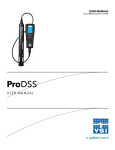
system and to use "accuracy" as indicating both the degree of precision and bias (see Figure 1).
For the purpose of this document, the term "accuracy" will be used to encompass “bias”.
Procedures to insure accuracy are described in Chapters 3, 4, and 5. As an example, accuracy can
be assured by instrument calibration and comparisons with external standards. Accuracy can also
be gauged by an independent measurement such as a contracted laboratory identification of
macroinvertebrate samples first identified in-house.
Accuracy can also be assessed by analyzing “blank” samples. This verifies that the measured or
analyzed value is true and not influenced by the sampling method or equipment. One equipment
blank sample should be submitted for each sampling expedition. Blank water should be drawn
from the sinks equipped with deionizing system taps in the laboratory. Volatile organic
compound (VOC)-free water, available in the organic laboratory, should be used for blanks for
VOC analyses. Blank water should be processed and transported exactly as are regular samples.
All field water quality measurements except dissolved oxygen should be performed on blank
samples.
Representativeness
Collecting a sample representative of the true environmental conditions requires proper sampling,
handling, preservation, and transport. Refer to Chapters 3 and 4 for specific sample collection
procedures and field analyses. Refer to the FSRG for required containers, volumes, preservation,
blanks, and holding times for specific analyses. Sample representativeness is also discussed in
Chapter VIII (Sample Collection) of the FSRG.
Quality Assurance
DEQ03-LAB-0036-SOP
Water Monitoring and Assessment Mode of Operations Manual
Chapter 2 General Considerations
Oregon Dept. of Environmental Quality
Date: 3/10/2009
Page 5 of 33
Figure 1: Precision, Bias, and Accuracy
Comparability
Data comparability is essential to interpret results from samples collected at different times and
locations. Carefully following documented procedures is one of the most important steps in
maintaining data comparability. Use approved EPA methods whenever possible. Refer to
Chapters 3, 4, and 5 for guidance on specific procedures and analyses.
Completeness
Completeness of a study is based on a comparison of the amount of valid data expected and the
amount actually generated from the study. Before a project begins, the project manager or data
user should decide how much data are needed to answer the project questions and what is the
minimum percentage of expected data that will be useable. While there are no specific QA
procedures to assure project completeness, following a QA program will increase completeness
by lessening the amount of data discarded for insufficient certainty. It may also be appropriate to
budget a small amount of oversampling if there is an expected or assumed rate of incompleteness.
Quality Assurance
DEQ03-LAB-0036-SOP
Water Monitoring and Assessment Mode of Operations Manual
Chapter 2 General Considerations
Oregon Dept. of Environmental Quality
Date: 3/10/2009
Page 6 of 33
Data Quality Matrix
Data generated from the laboratory is graded based on its quality, Levels A+ through F. These
criteria are summarized for field water quality parameters in the Data Quality Matrix (See
APPENDIX A at the end of this Chapter). The most current version can be found on QNet or
by clicking on this hyperlink DEQ04-LAB-0003-QAG). Data Quality Matrix Limits should be
defined in applicable QAPP. Data quality also depends on other factors as described in a
QAPP, as discussed in Chapter 2, Project Planning.
Documentation
The quality of data often depends not on the analysis, collection, or measurement, but the
documentation that accompanies (or doesn’t accompany) the sample. Obvious examples are
sample location, time, date, and required analyses. The FSRG details required documentation
such as Request for Analysis forms and non-routine documentation such as chains-of-custody.
For routine ambient water quality sampling, measurements are only recorded on field data sheets
for the DEQ Lab and the Public Health Lab (for microbiological samples). Bound field
notebooks are kept for projects and this allows sampling events to be reconstructed and
documentation of additional metadata that have no place on the field sheets. All documentation
should be in ink. Corrections should be made by drawing a single line through the mistake,
writing in the correction, and initialing the correction. Documentation of weather conditions and
all anomalous conditions, such as extremely high or low flow or bulldozers in the stream, will
assist in data interpretation.
Following the concepts outlined in this section, as well as the remaining documentation in MOMs
and other referenced material, assures that data becomes high quality information. Remember
that the samples we collect will be used to inform decision-makers and to educate the public.
References
Oregon DEQ, December 1997. State of Oregon DEQ Quality Assurance Management Plan,
Oregon DEQ Laboratory, Portland, Oregon.
Oregon DEQ, July 1998. DEQ Laboratory Quality Assurance Plan, Oregon DEQ
Laboratory, Portland, Oregon.
Oregon DEQ, December 1998. DEQ Field Sampling Reference Guide, Oregon DEQ
Laboratory, Portland, Oregon.
Oregon DEQ, February 2004. Data Quality Matrix Version 3.0, DEQ04-LAB-0003-GD, Oregon
DEQ Laboratory, Portland, Oregon.
Oregon DEQ, State of Oregon DEQ Quality Management Plan, Oregon DEQ Laboratory,
Portland, Oregon. DEQ03-LAB-0006-QMP.
US EPA, Office of Wetlands, Oceans, and Watersheds, September 1996. The Volunteer
Monitor’s Guide to Quality Assurance Project Plans. EPA 841-B-96-003. Washington, DC.
Quality Assurance
DEQ03-LAB-0036-SOP
Water Monitoring and Assessment Mode of Operations Manual
Chapter 2 General Considerations
Oregon Dept. of Environmental Quality
Date: 3/10/2009
Page 7 of 33
PROJECT PLANNING
The DEQ Quality Management Plan (QMP) describes the use of Quality Assurance Project Plans
and Sampling and Analysis Plans within DEQ.
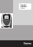
Projects within DEQ that generate, acquire, and use environmental data follow a generic threestep life-cycle: (1) planning; (2) implementation and oversight; and (3) assessment and
improvement (Figure 2).
Figure 2 DEQ Project Life-cycle (from QMP, Figure 4)
Project Planning
DEQ03-LAB-0036-SOP
Water Monitoring and Assessment Mode of Operations Manual
Chapter 2 General Considerations
Oregon Dept. of Environmental Quality
Date: 3/10/2009
Page 8 of 33
Careful attention to quality issues at each stage in the life-cycle is crucial for ensuring that project
data is of the quality required for informed decision making. Moreover, the project life-cycle is
iterative in nature, feeding valuable quality information back into itself and other projects for
constant system improvement. The scope of this simplified project model applies to all
environmental monitoring and measurement activities mandated by State or Federal Regulations,
or memoranda, and includes environmental data generated both internally and externally by
activities conducted through Agency programs, contracts, inter-agency agreements, grants, and
cooperative agreements.
Quality assurance at the project level is a dynamic system in which two basic elements--quality
control and quality assessment--form a positive feedback loop. Once a project's data quality
objectives (DQO’s) are defined during planning, effective operation of the Quality System
requires that quality control procedures are integrated into the overall data generation process.
See the previous chapter on Quality Assurance for a further discussion of data quality objectives.
The QC data are then used to decide whether the desired data quality objectives are being
achieved and, if not, to establish a basis for any corrective actions that may be needed. To assure
that these activities are a routine part of all data collection efforts, all environmental monitoring
and measurement activities within the scope of the Quality Management Plan must be defined in
a Quality Assurance Project Plan (QAPP).
Quality Assurance Project Plans
The Quality Assurance Project Plan (QAPP) is the core project level component in the Quality
System and, consequently, is a required element. The QAPP integrates all technical and quality
aspects of a project, including planning, implementation, and assessment. The purpose of the
QAPP is to systematically document project activities and provide a defined plan for obtaining
the type and quality of environmental data needed for a specific decision or use. The QAPP
documents how quality assurance (QA) and quality control (QC) activities are applied to ensure
that project results are of the type and quality needed for the intended use of the data. The QAPP
addresses all monitoring operations, including field and laboratory activities, which generate data,
as well as data storage, retrieval, and assessment. QAPPs must be written for all DEQ projects
regardless of whether or not data is generated internally within DEQ or externally from thirdparties or partners outside the Agency. DEQ's requirements for QAPPs are equivalent to those
required by EPA. The elements of the QAPP fall within four major project categories:
(1)
(2)
(3)
(4)
Project Management;
Data Generation and Acquisition;
Assessment and Oversight; and
Data Validation and Usability.
A number of specific elements must be addressed in the QAPP to fully document the project's
planned activities. The minimum elements that must be addressed in the QAPP include:
(1) Project Management Elements:
• Title and Approval Sheet
• Table of Contents
• Distribution List
• Project/Task Organization
• Problem Definition/Background
• Project/Task Description
• Quality Objectives and Criteria
• Special Training/Certification
• Documents and Records
Project Planning
DEQ03-LAB-0036-SOP
Water Monitoring and Assessment Mode of Operations Manual
Chapter 2 General Considerations
Oregon Dept. of Environmental Quality
Date: 3/10/2009
Page 9 of 33
(2) Data Generation and Acquisition Elements:
• Sampling Process Design
• Sampling Methods
• Sample Handling and Custody
• Analytical Methods
• Quality Control
• Instrument/Equipment testing, Inspection, and Maintenance
• Instrument/Equipment Calibration and Frequency
• Inspection/Acceptance of Supplies and Consumables
• Non-direct Measurements
• Data Management
(3) Assessment and Oversight Elements:
• Assessments and Response Actions
• Reports to Management
(4) Data Validation and Usability Elements:
• Data Review, Verification, and Validation
• Verification and Validation Methods
• Reconciliation with User Requirements
Complete details on QAPP requirements can be found in EPA QA/R-5 EPA Requirements for
Quality Assurance Project Plans (US EPA, 2001). Copies of this document are available from
the EPA web site and the DEQ intranet. DEQ-specific guidance on the development and writing
of QAPPs is in development and will be posted to Q-net when it becomes available. All Agency
QAPPs must be reviewed by the QA Officer (QAO) or designee. Individual divisions and offices
within the Agency are responsible for ensuring that all QAPPs are approved prior to the
commencement of any work and that project activities are implemented as documented.
Individual division and offices are responsible for maintaining copies of the approved QAPPs.
However, electronic copies of all approved QAPPs should be submitted to the QAO (preferably
in PDF format), who will maintain a library of QAPPs and post electronic copies to the DEQ
internet.
Sampling and Analysis Plans
In many cases a generic QAPP may be written that covers many DEQ projects/activities where
only specific details (e.g., sampling locations, measurement parameters, etc.) change. For these
projects, abbreviated Sampling and Analysis Plans (SAPs) may be substituted in lieu of a
complete new QAPP. However, the SAP must reference the parent QAPP and may not make
substantial changes to the DQOs established in the parent document. The use of a SAP in lieu of a
QAPP is valid for data that is generated internally within the Agency only. All projects involving
data generated from external or secondary sources must be documented in a QAPP.
SAPs should be used only to specify changes in sampling location and monitoring data. If
additions or deletions to a project's monitoring requirements are such that the QA or QC activities
documented in the parent QAPP are compromised, a new QAPP must be written and approved.
SAPs must be submitted to and approved by a QAC prior to the commencement of any project
work. It the responsibility of the originating division and/or office to ensure that the requirements
specified in the QAPP are satisfied. Electronic copies of SAPs should be submitted to the QAO,
who will maintain a library of SAPs with the parent QAPPs and post them to the internet.
Project Planning
DEQ03-LAB-0036-SOP
Water Monitoring and Assessment Mode of Operations Manual
Chapter 2 General Considerations
Oregon Dept. of Environmental Quality
Date: 3/10/2009
Page 10 of 33
Analysis Request Forms
All planned sampling events of any size must be documented using an Analysis Request Form
before sampling occurs. These Analysis Request Forms provide the laboratory a list of sample
quantity, sample media, requested analyses, date of sampling and delivery, QA samples required,
and requested date for data reporting. An Analysis Request Form also identifies the project
manager, their telephone number, and fund code to which sample analysis should be charged.
See the “Sample Collection Activity Meta-Data” portion of the following “Data Management”
section for a discussion of required data elements.
References
Oregon DEQ, DEQ Quality Management Plan, Version 4.1, DEQ03-LAB-0006-QMP Oregon
DEQ Laboratory, Portland, Oregon.
US EPA, 2001. EPA Requirements for Quality Assurance Project Plans (EPA QA/R-5).
EPA/240/B-01/003, Office of Environmental Information, US EPA, Washington, DC.
Project Planning
DEQ03-LAB-0036-SOP
Water Monitoring and Assessment Mode of Operations Manual
Chapter 2 General Considerations
Oregon Dept. of Environmental Quality
Date: 3/10/2009
Page 11 of 33
DATA MANAGEMENT
Introduction
High-quality data management is as important to a project as is high quality sampling and
analysis. Improperly handled data can result in misreporting or omission of data, ultimately
leading to misinformed water quality management decisions. While this concept is generally
appreciated by those involved in watershed assessment projects, scant resources have been
allocated to data management. “Data Management” includes time spent collecting and recording
sample project and sample event meta-data, creating new stations in the database, entering field
and laboratory data, verifying data, performing QA/QC checks on data, and transferring data
between various databases. Spending the time and resources necessary to assure high-quality
data management will maintain the integrity and total quality management of any water quality
project.
Following Standard Operating Procedures for collecting and analyzing water quality samples
assures high quality analytical results. In order to transfer these high-quality analytical results
into high-quality information, methods for managing the data and information products should
also be standardized. Data management, for the purposes of this discussion, begins when the
analytical result is transferred to the recording medium (paper or electronic) and ends when the
validated data are verified as complete and accurate in their ultimate destination. That destination
is a data repository that is easily accessible to persons interested in the data. Presently, validated
data are released from LIMS (Laboratory Information Management System) to LASAR
(Laboratory Analytical Storage and Retrieval) and then uploaded to STORET (EPA’s STOrage
and RETrieval).
LASAR data are available at http://deq12.deq.state.or.us/lasar2/
STORET data are available at http://www.epa.gov/storet/dbtop.html.
The Laboratory’s Technical Services section is largely responsible for data management. Sample
tracking, LIMS/LASAR development and management, and related documentation and support
are among the services provided by this section. Contact Technical Services for the most current
information regarding data management.
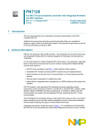
A graphical representation of the data management process for WA section data is given in
Figure 3 and Figure 4
Data Management
DEQ03-LAB-0036-SOP
Water Monitoring and Assessment Mode of Operations Manual
Chapter 2 General Considerations
Oregon Dept. of Environmental Quality
Date: 3/10/2009
Page 12 of 33
Figure 3 (Sample Collection to Sampling Event Data Entry Complete)
Sample Collection
Sample
Preservation
Field Analysis
Record Field
Data
Transport to Sample
Tracker
Yes
New
Station
No
Tracker
Assigns
Analyses
Station Information
entered in LIMS,
LASAR and
STORET
Field Data
entered in LIMS
Field Staff corrects
errors in LIMS
Yes
Laboratory
Analyses
Analytical Data
entered in LIMS
Field Staff review Data
Approval Report (DAR)
Lab Workgroup
generates analytical
QA/QC reports
Errors
Laboratory Analytic Review
of LIMS data and QA/QC
reports, corrective action as
necessary
No
Sampling Event Data
Entry Complete
Data Management
DEQ03-LAB-0036-SOP
Water Monitoring and Assessment Mode of Operations Manual
Chapter 2 General Considerations
Oregon Dept. of Environmental Quality
Date: 3/10/2009
Page 13 of 33
Figure 4 Data Management Flowchart
(Sampling Event Data Entry Complete to Storage in STORET)
Sampling Event Data
Entry Complete
Technical Services
generates QA/QC report
QAO reviews LIMS data and
QA/QC Report
Lab Administrator approves
LIMS Sampling Event Report
Sampling Event
Released from LIMS
PDF Copy to Network
Storage and requestors,
Hard Copy to File
LASAR DBA
transfers Data to
LASAR
WA Data Manager
(DM) assigns data
verification to WA
Staff
WA Staff verifies
completeness and
accuracy of data
WA staff returns sampling
event data to WA DM with
comments/corrections
WA DM corrects
errors in LASAR
Yes
Errors
No
WA DM
transfers LASAR
Data to STORET
WA DM spot-checks
case in STORET
WA DM periodically
uploads to Nat’l STORET
Data Management
DEQ03-LAB-0036-SOP
Water Monitoring and Assessment Mode of Operations Manual
Chapter 2 General Considerations
Oregon Dept. of Environmental Quality
Date: 3/10/2009
Page 14 of 33
LIMS Sample Event Creation and Data Verification
This discussion assumes that an approved QAPP and/or SAP exists for the monitoring project. If
new stations and/or test methods will be established, enter as much information regarding the
stations or methods as possible into LIMS prior to samples arriving at the lab.
After samples are taken and/or field data are recorded, these are transported to the sample tracker.
The sample tracker assigns a Sampling Event (formerly known as LIMS Case) number to the
collected samples and/or data and assigns analyses to the chemistry sections. If the sample is
from a new station not yet in the database, the sample tracker informs the sample collector or
other appropriate person, who creates the new station in LIMS. The sample cannot be released
from LIMS until they can be assigned to a sample station.
After field data are entered into LIMS, the sample tracker scans the field sheets into LIMS.
Scanning the field sheets enables tighter control of data sheets after data is entered into LIMS.
The sample collector (or other responsible party) is responsible for comparing the LIMS Data
Approval Report (DAR) to the scanned field data sheet to ensure that the entered field data are
complete and accurate. This data review extends to ensuring that sample location, date, and time
were recorded correctly. The sample collector is responsible for either making corrections or
ensuring that corrections are made. The sample collector approves the DAR in LIMS, stating that
it is complete and accurate.
Meanwhile, chemists perform assigned analyses and enter the data into LIMS, after which a
Laboratory DAR is generated. The chemistry sections also perform QA/QC analyses applicable
to the individual method. After the appropriate chemistry sections have reviewed their data and
QA/QC data and performed corrective activities as necessary, data entry for the sample event is
considered complete.
When sample event data entry is complete, the QAO reviews LIMS data and QA/QC Reports for
the sample event, and passes the Sampling Event to the Lab Administrator who approves the
LIMS Sampling Event Report. If approved by the Lab Administrator, the Sampling Event report
is released to the public. Agency contacts will receive an e-mail notice with a hyperlink to a PDF
copy of the analytical report. Recipients must specifically request to receive reports in a different
format. The sample event data are uploaded to LASAR.
The WA Data Manager (DM) assigns data verification for the sample event to the sample
collector or other appropriate party. This data review by the monitoring staff member will verify
data completeness and accuracy for the sampling event. Monitoring staff should complete data
verification as quickly as possible to minimize time that erroneous data are available to the
public. Since the sample collector is most familiar with the source of the sample and the
conditions under which it was taken, the sample collector will be more likely to find data reported
with incorrect units, wrong order of magnitude, or otherwise not reasonably close to the expected
value. It is the responsibility of the sample collector to resolve the error, if it is an error, and
report all findings to the WA DM. The WA DM makes corrections to the data, as necessary.
The WA DM transfers data from LASAR to the local copy of STORET and spot-checks the
transfer in STORET. The WA DM periodically uploads the local copy of STORET to the
National STORET Warehouse.
Continuous Monitoring Variation
Continuous monitoring equipment is used to gain a more thorough understanding of variability of
certain water quality parameters than can be obtained through grab sampling. Using various
Data Management
DEQ03-LAB-0036-SOP
Water Monitoring and Assessment Mode of Operations Manual
Chapter 2 General Considerations
Oregon Dept. of Environmental Quality
Date: 3/10/2009
Page 15 of 33
types of equipment, parameters monitored in this manner include water and air temperature,
water depth, pH, dissolved oxygen, conductivity, salinity, turbidity, relative humidity, and solar
radiation. While operation of these various types of equipment differs, data management and
QA/QC concerns are similar.
Prior to deployment, the continuous monitoring equipment undergoes pre-deployment checks in
the laboratory to assure that the parameters of interest can be accurately measured. Upon
deployment in the field, the equipment is allowed to equilibrate to ambient conditions. Then the
parameter monitored is independently measured (audited) to assure that ambient conditions are
accurately measured by the continuous monitoring equipment. Audits are conducted at specified
times during the length of the deployment and just prior to retrieval from the monitoring site.
Although auditing can be time-intensive, higher frequency auditing provides higher data quality
assurance. The more important the data collected are, the higher frequency field staff may
consider performing audits. In addition to field audits, duplicate monitoring equipment may be
deployed for QA purposes or at sites where there is concern that equipment may be lost or stolen.
Duplicate equipment may also be deployed at sites deemed of critical importance where a backup
data source is desired in case of equipment failure.
After continuous monitoring equipment is retrieved from the field, a reasonable number of
monitoring stations/equipment is submitted together as a “Sampling Event”. A Required Report
Form serves as a cover sheet for the entire report. For the requirements to properly define the
data contained in the continuous monitoring sample event, see the section on meta-data. The
sample tracker assigns a sample event number. If one of the monitoring stations is new and not
yet in the database, the station must be created in LIMs prior to release of the data.
Data are downloaded from the equipment and checked against audit values for QA/QC. Each
data point receives a grade based on comparison to the audit value and pre-deployment/postretrieval accuracy checks. Data points failing audit and prior data back to the previous successful
audit will be omitted, leaving a sample time and a grade “C” accompanying the omission. For
each monitoring station and each piece of equipment, a graph of the data with superimposed audit
values and error bars is printed. Also printed is a QA/QC report summarizing results for that
piece of equipment. This information will allow the operator to determine whether anomalies
exist in the data, including equipment malfunctions and emergence of the equipment from the
water due to low flow. The operator will modify the data or the grade of the data based on this
review of data. Sample time recorded from the continuous monitoring equipment is standardized
to Pacific Standard Time, but can be retrieved as either Standard or Daylight Savings time to
synchronize with grab sample data.
After the data and grades are uploaded to LIMS, they are spot-checked to assure that the data
transfer was error-free. The QA/QC report is reviewed by the WA Section Manager or designee,
the QAO, and the Laboratory Administrator prior to release of the data to LASAR. These data
are spot-checked in LASAR. The WA DM transfers data from LASAR to the local copy of
STORET and spot-checks the transfer in STORET. The WA DM periodically uploads the local
copy of STORET to the National STORET Warehouse.
For further information about continuous monitoring data management, please see the Continuous
Data Quality Control and Quality Assurance section of Chapter 5 - Continuous Monitoring
Methods.
Sample Collection Activity Meta-Data
With the exception of ambient surface water quality monitoring network sampling, WA
sampling projects tend to be non-routine in terms of why and where the samples were
Data Management
DEQ03-LAB-0036-SOP
Water Monitoring and Assessment Mode of Operations Manual
Chapter 2 General Considerations
Oregon Dept. of Environmental Quality
Date: 3/10/2009
Page 16 of 33
taken. It is important to obtain sufficient meta-data (i.e., information about the data that is
collected) to allow users to make full and effective use of the data, and understand the
quality of the data over time. WA staff generally submits data sheets that are unique to the
project. It would be preferred to standardize data sheets, as much as possible, so that the
sample tracker can easily find these data elements and more efficiently do his/her job.
The following data elements must be submitted along with field analytical results and
sample container numbers.
1) Sample Subproject Code, LIMS/LASAR classification of the monitoring
activity, as stored in the Sample Subproject Table. The Sample Subproject table also
stores the Subproject’s SAP. Each Subproject shall have an SAP.
2) Station ID Code. This is the LASAR Station number and it relates to a STORET
Number, if applicable.
3) Station Name
4) Location, if the station is new. Latitude and longitude, either in degrees, minutes,
seconds or in decimal degrees. Include the method used to obtain this
information, including datum and map scale if applicable.
5) Elevation, in feet. If the station is new, indicate method used to obtain this
information.
6) River mile, where applicable.
7) Sample depth, where applicable. This is reported for groundwater monitoring,
typically, as two pieces of data: depth to bottom and depth to water. For surface
water, this is reported when sampling at non-standard depths, such as during
horizontal profile sampling, or when sampling at Secchi depth in lakes or
estuaries.
8) Date of sample collection. Use MM/DD/YYYY format (Example: 05/31/1999).
9) Time of collection. Use the 24 hour clock and HH: MM format (Example: 14:35
to designate 2:35 p.m.). Report all sample times as either Pacific Standard or
Pacific Daylight Savings Time.
10) Method(s) used in sample collection, if non-standard. The method should be
specified in the sample project’s QAPP or SAP.
11) Sampling equipment type and tag number.
12) Sample Matrix. This describes the physical state of the sample, i.e., “surface
water”, or “sediment”.
13) Sample Classification, i.e., trawl, time composite, area composite, volume composite,
continuous, or grab.
14) QA/QC Classification, i.e., equipment blank, QA duplicate, etc.
15) Sample Comments. Any comments, if appropriate.
Field Analysis and Data Collection
Most WA section field data collection relies on either direct observation (or estimation),
instrumental analysis, or chemical analysis of the environmental variable. In order to assure the
highest quality data, staff should carefully consider analytical uncertainty and significant digits,
rounding error, and units of measurement. More on this subject can be found in Bevington and
Robinson (1992).
Data Management
DEQ03-LAB-0036-SOP
Water Monitoring and Assessment Mode of Operations Manual
Chapter 2 General Considerations
Oregon Dept. of Environmental Quality
Date: 3/10/2009
Page 17 of 33
Analytical Uncertainty and Significant Digits
Any measurement is prone to error; thus, it is impossible to be certain that our result is a true
measurement of the environmental variable under consideration.
Blunders
One class of errors originates from blunders in measurement or computation. Blunders are
usually obviously incorrect or not reasonably close to expected values, and can be eliminated by
careful re-measurement or recalculation.
Accuracy and Systematic Errors
Accuracy is a measure of how close the observed value is to the true value. Accuracy is
dependent on how well we can control systematic errors, such as faulty equipment calibration or
observer bias, which make our results different from the true value with reproducible
discrepancies. Systematic errors may be reduced by maintaining strong QA/QC and training
programs and regular equipment maintenance.
Precision and Random Errors
Precision is a measure of how well the result has been determined, regardless of its accuracy. It is
also a measure of the reproducibility of the result. Precision is dependent on how well we can
compensate for random errors, such as instrumental error or subsample variation, which cause
results to vary between observations. Random errors may be reduced by improved methods,
refined technique, improved instrumentation, or by repeated measurements.
Accounting for Uncertainty
Perhaps the best way to account for analytical uncertainty is to quantify and document it as part
of the analytical result. For example, by performing multiple measurements on a series of
standards, a chemist can derive a standard curve relating observed measurement to analyte
concentration, within a quantified estimate of error. This can be expressed as absolute precision
(i.e., 1.979 mg/L ± 0.012 mg/L) or as relative precision (i.e., 1.979 mg/L ± 0.6%). The reality of
a fast-paced working environment precludes such circumstantial determinations of uncertainty.
WA section uses methods with documented acceptable error levels, analytical equipment that can
read a standard solution within an acceptable error level, and other QA/QC checks (i.e., blank and
duplicate analyses) to minimize uncertainty. However, the remaining uncertainty is not
documented with the analytical result. Another way to account for analytical uncertainty is to be
conservative in the way the result is reported. When using electronic analytical equipment, the
analyst’s first instinct is to report the value (i.e., 4.74 NTU) displayed by the instrument without
first considering analytical uncertainty. Following this instinct places more confidence in the
least significant digit than is prudent. Table 1 describes the accuracy of typical field analyses and
requirements for reporting results. This table should be used as a guideline for determining how
to report results for other analyses.
Table 1 Requirements for Reporting Field Analysis Results
Analysis
DO concentration
Method or
Instrument
Winkler Titration
DO Saturation
Calculation
Scale
Rel. Precision
Data Management
Abs. Precision
Recommendation
±0.1 mg/L
Report to tenths
0.7-1.4%
Report whole units
DEQ03-LAB-0036-SOP
Water Monitoring and Assessment Mode of Operations Manual
Chapter 2 General Considerations
Analysis
pH
Method or
Instrument
Digital meter,
combination electrode
with ATC probe
Scale
Oregon Dept. of Environmental Quality
Date: 3/10/2009
Page 18 of 33
Rel. Precision
Abs. Precision
Recommendation
±0.1 SU
Report to tenths
Alkalinity
Potentiometric (pH)
titration
±1.0 mg/L
Report whole units
Temperature
YSI Model 30
±0.1°C
Report to tenths
Conductivity
YSI Model 30
0-499.9
µmhos/cm
±2% Full Scale
±10
max
µmhos/cm
Report 2 sig. digits
YSI Model 30
0-4999
µmhos/cm
±2% Full Scale
±100 µmhos/cm
max
Report 2 sig. digits
YSI Model 30
0-49.9
mmhos/cm
±2% Full Scale
±1
mmhos/cm
max
Report 2 sig. digits
YSI Model 30
0-200
mmhos/cm
±2% Full Scale
±4
mmhos/cm
max
Report 2 sig. digits
Salinity
YSI Model 30
0-80 ppth
±1.6 ppth max
Turbidity
Hach 2100P
Turbidimeter
0-10 NTU
±2% FS or 0.1
ppth
±2% Full Scale
Report up to 2 sig.
digits
Report 1 sig. digit
Hach 2100P
Turbidimeter
0-100 NTU
±2% Full Scale
±2.0 NTU
Report 2 sig. digits
Hach 2100P
Turbidimeter
0-1000 NTU
±2% Full Scale
±20 NTU
Report 2 sig. digits
±0.2 NTU
(<1.0 NTU)
(Report“<1 NTU”)
Rounding Error
Misunderstanding rounding rules leads to systematic errors in reporting values either too high or
too low. To round off a number, note the number to the right of the desired least significant
figure. Compare to the number 5, or 50, or 500, etc., depending on the number of digits to the
right of the desired least significant figure.
1) If the number is greater, increase the least significant figure by 1. Example: To
report two significant digits, 175.1 becomes 180.
2) If the number is less, leave the least significant figure as is. Example: To report two
significant digits, 174.9 becomes 170.
3) If the number is equivalent, increase the least significant figure by 1 if it is odd or
leave it as is if it is even. Example: To report two significant digits, 175.0 becomes
180 and 185.0 becomes 180.
Using the third rule as the convention reduces systematically high or systematically low values
that would otherwise influence the average of a group of such numbers. In short, round to even.
Data Management
DEQ03-LAB-0036-SOP
Water Monitoring and Assessment Mode of Operations Manual
Chapter 2 General Considerations
Oregon Dept. of Environmental Quality
Date: 3/10/2009
Page 19 of 33
Units of Measurement
The importance of reporting correct units of measurement cannot be overstated. Inattention to
such detail as conversion of units between metric and English systems of measurement led to the
crash of the Mars Climate Orbiter into the surface of Mars. While our mission is not as critical,
entry of salinity as “ppt” has led to reporting salinity as parts per trillion, rather than parts per
thousand (ppth), nine orders of magnitude difference. Ensure that units of measurement are
clearly marked on the field analysis sheet and that they are properly entered into the database.
When verifying the accuracy and completeness of collected data, ensure that the units and/or
order of magnitude of the result are correct.
In summary, WA staff is responsible for providing required meta-data elements, as well as
carefully considered field analytical results. This provides a high-quality foundation upon which
subsequent analyses are based.
References
Bevington, Philip R. and D. Keith Robinson, 1992. Data Reduction and Error Analysis for the
Physical Sciences, Second Edition. McGraw-Hill, Inc., San Francisco, California.
Data Management
DEQ03-LAB-0036-SOP
Water Monitoring and Assessment Mode of Operations Manual
Chapter 2 General Considerations
Oregon Dept. of Environmental Quality
Date: 3/10/2009
Page 20 of 33
DATA ANALYSIS
Department staff uses Water Monitoring and Assessment data for a variety of purposes. Some of
the routine uses are identified below.
All data is evaluated every two years to determine the extent to which surface and ground water
bodies meet water quality standards and types of impairment. This evaluation is a major part of
the preparation of the Water Quality-Limited Streams 303(d) list, as well as the Water Quality
Status Assessment 305(b) Report.
Much of the data collected is used by regional watershed specialists and TMDL modelers to
develop and assign load and waste load allocations. The collected data serves as ground-truthing
information for GIS and numeric water quality models. Ground-truthing is an analysis of the
validity of GIS data and model information. As the agency moves to a water quality based
permitting approach, NPDES permit writers will evaluate water quality data for receiving streams
prior to issuing new or renewed permits.
Ambient river monitoring data is used to develop an Oregon Water Quality Index (OWQI) score
for every sample. The water quality index data is then used to rank sites, identify spatial and
temporal variability, and communicate water quality conditions to the public. Ten-year trending
analysis based upon the OWQI is conducted for all ambient network sites. Trend data is used to
measure progress and is a primary environmental indicator for the Performance Partnership
Agreement with EPA and the Oregon Progress Board Benchmarks Program.
Probabilistic sampling plans, such as the Oregon Plan for Salmon and Watersheds and Regional
and Coastal Environmental Monitoring and Assessment Programs (REMAP and CEMAP),
collect data from randomly selected locations in water bodies in selected areas. Indicators are
selected and measured to determine types of impairment, and cumulative distribution functions
are developed for each indicator for the study. This data is used primarily to:
•
•
•
•
Determine the status of conditions in water bodies critical to the survival and
recovery of threatened or endangered fish species across the state.
Identify trends in water body conditions within areas with listed fish species.
Identify chemical and physical parameters impairing water body conditions.
Help determine the effectiveness of restoration projects and changes in
management practices in improving conditions for listed fish species.
Data collected for Best Management Practices (BMP) monitoring, whether for surface or
groundwater, are evaluated to determine long-term trends and the effectiveness of the BMP plan.
Data are also collected to monitor water quality permit holders for compliance with water quality
standards. In this case, DEQ data are either directly compared to standards, or are collected
simultaneously with the permittee’s contracted monitoring organization for comparison to assure
their data are of sufficient quality.
It is imperative that data used for analysis are of known quality. The data should have
documented Precision, Accuracy, Representativeness, Comparability, and Completeness
(PARCC). More information on this topic can be found in the QA/QC section of this manual.
The data used for analysis should come from a sample design that allows for the desired
analytical use. The analyst should carefully choose numerical methods of analysis. See the
references listed below for guidance in environmental statistics. In this manner, the results of the
analysis and policies that may be evaluated or changed as a result, are based on defensible, sound
science.
Data Analysis
DEQ03-LAB-0036-SOP
Water Monitoring and Assessment Mode of Operations Manual
Chapter 2 General Considerations
Oregon Dept. of Environmental Quality
Date: 3/10/2009
Page 21 of 33
References
Gilbert, R. O., 1987. Statistical Methods for Environmental Pollution Monitoring. Van Nostrand
Reinhold Co., New York.
Helsel, D. R., Hirsch, R. M., 1991. Statistical Methods in Water Resources. Appearing as
Chapter A3 in Techniques of Water-Resources Investigations of the United States Geological
Survey Book 4, Hydrologic Analysis and Interpretation. US Geological Survey, Reston,
Virginia.
Sanders, T. G., R. C. Ward, J. C. Loftis, T. D. Steele, D. D. Adrian, V. Yevjevich, 1994. Design
of Networks for Monitoring Water Quality. Water Resources Publications, Highlands Ranch,
Colorado.
Data Analysis
DEQ03-LAB-0036-SOP
Water Monitoring and Assessment Mode of Operations Manual
Chapter 2 General Considerations
Oregon Dept. of Environmental Quality
Date: 3/10/2009
Page 22 of 33
SAFETY
One of the primary objectives of the Water Monitoring and Assessment Sections is to provide
high quality data so that the agency can make informed decisions. Unless the health and safety of
our staff is monitored and protected, the quality of our data will suffer. Healthy, alert monitoring
staff is better able to produce high quality work than is ill, injured, or groggy staff.
The DEQ Central Safety Committee and the DEQ Laboratory Safety Committee strive to meet or
exceed Oregon Occupational Safety and Health Administration (OR-OSHA) regulations to
protect our health while on the job. These programs are documented in the DEQ General Health
and Safety Policy, DEQ Health and Safety Program, the DEQ Laboratory Safety Manual
(Chemical Hygiene Plan), and the DEQ Laboratory Safety video. Hazards associated with
specific tasks and measures to mitigate those hazards are documented in Job Safety Assessments
(JSA), which are on file with the agency's Safety Coordinator. All staff must read the above
documentation and be trained. Such training must be documented. The purpose of this section is
to accentuate safety topics of particular interest to WA section staff.
General Safety
There are many hazards inherent to our jobs, whether we’re working in the laboratory, collecting
or analyzing environmental samples in the field, or transporting ourselves during monitoring via
motor vehicle, boat, hiking boot, or wader. In order to ensure that these hazards are recognized
and understood, all new employees are required to understand the contents of the documents
referenced above. In the case of the DEQ General Health and Safety Policy and Job Safety
Assessments, the employee’s signature documents that these policies are understood. All
employees should be familiar with the location of potential hazards and safety equipment in their
immediate workspace, throughout the lab, in vehicles and boats, and in the field.
Documentation: The DEQ General Health and Safety Policy is included in the packet of materials
given to new employees, and is also available in the laboratory front office area. Copies of the
DEQ Health and Safety Program and the DEQ Laboratory Safety Manual (Chemical Hygiene
Plan) are located in the laboratory front office area, and are also available from the Laboratory
Safety Committee representatives. The DEQ Laboratory Safety Video is available from the
Laboratory Chemical Hygiene Officer (and QAO). Job Safety Assessments are available from
your section’s Safety Committee representative.
All employees should be familiar with evacuation routes and designated assembly areas for their
work location. For the laboratory, the designated assembly area is in the parking are on the
Southwest side of the outbuilding. In case of evacuation, meet at the designated assembly area,
check in with your Emergency Coordinator (section safety committee representative, section
manager for back up), and remain with your group until further notification.
Laboratory Safety / Chemical Hygiene
When working in the lab or performing chemical analyses in the field, it is imperative that you
protect your eyes. Safety glasses are available at the lab. Prescription safety glasses will be
provided if necessary. Perhaps the best eye protection is given by vented goggles.
Hands and fingers are susceptible to chemical exposure due to their proximity to samples and
reagents. It is important to match the protective glove to the chemicals used. For most work
performed by our sections, PVC gloves are sufficient. Inspect and carefully handle glass bottles,
beakers, and other glassware to prevent cuts from chips or cracks.
Safety
DEQ03-LAB-0036-SOP
Water Monitoring and Assessment Mode of Operations Manual
Chapter 2 General Considerations
Oregon Dept. of Environmental Quality
Date: 3/10/2009
Page 23 of 33
Other areas of your body are also susceptible to chemical burns. Protect exposed skin with
clothes that you don’t mind damage to, or further protect your skin and clothes with a lab-coat or
coveralls. Personal protective equipment (PPE) will be provided by the lab.
Label all chemical containers so that personnel are cognizant of the container’s contents.
Information on labels should include chemical name, concentration if applicable, date filled,
expiration date, and initials of the person filling the container.
Chemical waste produced from our sections’ water quality analyses must be contained (if
produced in the field) and disposed of in any deep sink in the laboratory. Spent concentrated
acids and bases should be neutralized or diluted and flushed down the deep sink with excess
water: turn on a faucet in a laboratory sink and then slowly pour the chemical into the stream
of water to be flushed down the drain. Before discharge into the sewer this material passes
through a pH-monitored neutralization tank, maintained by the Department of Administrative
Services, this ensures neutralization. Other wastes, such as ethanol or formalin, require special
handling for which special procedures have been developed. Contact your Safety Committee
representative for more information. Under no circumstances should chemical waste be disposed
of in the field. Ensure you have adequate or excess waste container capacity before leaving for
field monitoring expeditions.
Documentation: For specific information regarding chemical reagents, refer to the chemical’s
Material Safety Data Sheet (MSDS). MSDSs are maintained in notebooks located in the
laboratory front office area.
Field Safety
All field staffs are required to complete First Aid and CPR training every two years. This ensures
that staff can care for each other in case of a medical emergency in the field. Additionally, field
staff responsible for spending long periods of time in remote areas may be trained (or
accompanied by a staff member that is trained) in wilderness first aid. This training will also be
updated every two years. These courses are typically offered by DEQ every June.
A significant portion of field monitoring activities is driving to monitoring locations. Fatigue
from long hours behind the wheel of a vehicle or boat puts monitoring staff at considerable risk.
Travel with a partner, whenever possible, to share driving responsibilities. Employees are to
avoid working long hours and driving while tired. Defensive driving courses are offered by DEQ
and are required of new employees responsible for driving state vehicles. The course must be
repeated every five years.
Boater Education is required before an employee can drive state boats. The Mandatory Boater
Education course is available from a variety of outlets. After completing the course, staff must
apply for a Boater Education card. This card must be carried at all times while operating a boat.
The card is good for life and the course has no continuing education requirement.
Work on bridges and on roadway shoulders exposes staff to hazards from passing vehicles.
Increasing your visibility to motorists, minimizing your exposure time, and keeping one eye on
approaching traffic are effective ways of minimizing risk. When working on the road, staffs are
required by OR-OSHA (OR-OSHA, 2001, OAR 437-003-0128) to wear an article of highvisibility clothing (such as a vest); viewable from 360° (open-sided vests are obsolete). If
lighting is poor or visibility is low, use a vest with reflective tape. Where possible, position your
vehicle between approaching traffic and the work site. Use flashing/rotating lights on your
vehicle and station a “Workers Ahead” sign between approaching traffic and the work site. Stage
safety cones in advance of your work zone, whether it is on the bridge or on the roadway
Safety
DEQ03-LAB-0036-SOP
Water Monitoring and Assessment Mode of Operations Manual
Chapter 2 General Considerations
Oregon Dept. of Environmental Quality
Date: 3/10/2009
Page 24 of 33
shoulder. Taper the cones from the edge of the shoulder furthest from the roadway, or from the
bridge railing, to the fog line on the roadway. The distance between the cones in the taper should
equal in feet the designated speed, e.g., 55 mph = 55 feet (ODOT, 1998). The intent of safety
cone staging is to alert the motorist’s attention to work zone activity and to direct the motorist to
drive away from the work zone. Plan your work to spend the least amount of time possible on the
bridge or on the shoulder. When on the bridge, employ one monitoring staff as a “spotter”. The
spotter keeps an eye on traffic while the other staff draws the sample. If visibility is limited or
traffic is especially heavy or fast, consider staging the spotter at the end of the bridge. Use of a
whistle or two-way radio is an effective means of communicating the approach of potentially
hazardous motorists. While drawing the sample from the bridge, take great care. Slipping and
falling off the bridge could be fatal.
Sampling from a boat poses its own challenges. One person onboard should be responsible for
monitoring boat traffic and weather/water conditions both visually and on the radio. OR-OSHA
requires (OR-OSHA, 2001, OAR 437-002-0139) that personal floatation devices (PFDs) are worn
at all times. When maneuvering the boat trailer at the boat ramp, or in other cramped
maneuvering spaces, clear communications must be maintained between the driver and the trailer
spotter on the ground. Towing a boat or other pieces of monitoring equipment requires that the
driver be familiar with associated hazards including longer distances to stop and safety equipment
such as safety chains and proper trailer lighting.
When sampling from the bank, from a boat dock, or instream, where the danger of drowning
exists and water is greater than five feet, OR-OSHA requires (OR-OSHA, 2001, OAR 437-0021139) that personal floatation devices be worn.
Hiking/backpacking, wading, and climbing to or along monitoring sites exposes staff to injuries
from falls, sprains/strains, stick-pokes, bites, stings, etc. Due care should be taken while working
far afield due to the distance from medical facilities. A two-day wilderness first aid course is
available to staff who work in those conditions.
Backpack electro-shockers are used to stun and collect fish in wadeable streams. There is a risk
of shock to personnel instream when electro-shocking is underway. All personnel instream
should wear waders that are electrically insulating. Staff performing electro-shocking should
keep their eyes and ears open for the possibility of another staff slipping and falling into the water
and receiving a shock.
Staff involved in sampling at hazardous waste sites will receive training on the selection and use
of respirators and other Personal Protective Equipment (PPE). They will also receive training on
Hazard Communications. They will also be properly fitted with respirators and receive medical
monitoring to ensure that any exposure to hazardous chemicals is detected and cared for. These
staff will also be advised on safety plans that are specific to the sites they visit.
Field staff must carry a cell phone or satellite phone into the field. Staff must call into the lab
every day, preferably near the end of the day, to check in. Staff should leave a message with their
manager (if available), or front office staff, or on the lab’s general message voice mail. Staff
should advise of their location, health status, projected activities for the next day, and any other
pertinent information. Using these measures, communications between field staff and the lab will
be more feasible in the event of emergency. If field staffs fail to check in and it is feared that they
may have been involved in an accident, it will enable lab staff to more precisely locate field staff
for emergency personnel.
Safety
DEQ03-LAB-0036-SOP
Water Monitoring and Assessment Mode of Operations Manual
Chapter 2 General Considerations
Oregon Dept. of Environmental Quality
Date: 3/10/2009
Page 25 of 33
Accidents
Accidental spills of hazardous chemicals can pose a significant risk to staff. Spills of small
quantities (less than 15 L) that are of minimal health risk can be contained, neutralized, or
collected using absorbent materials by our staff. Consult the Laboratory Emergency Operations
Plan (DEQ, 2002) and applicable MSDS for appropriate clean-up methods and PPE. For large
spills, evacuate the area and call 911.
For any accident involving personal injury, seek first aid or medical attention immediately and
inform your manager regarding severity. DEQ requires that an Accident/Incident Report, "Form
DEQ 34", available from the Front Office, be filed with 24-hours following an accident or
incident where the potential for injury could have occurred. When medical treatment is required
for a work-related injury or illness, fill out a State of Oregon Worker's and Employer's Report of
Occupational Injury or Disease, SAIF Corporation, Form 801, available from the Front Office.
The supervisor must complete this report and mail or fax it to SAIF and Human Resources. This
report must be provided to SAIF within 36 hours of the incident.
Conclusion
Safety regulation, training, and documentation will be effective in minimizing workplace
accidents and injuries only when combined with working carefully and paying attention to the
task at hand. If working conditions are dangerous, consider postponing your work until
appropriate safeguards are in place. If you any questions or concerns regarding safety, contact
your section Safety Representative and/or manager.
References
Oregon Department of Environmental Quality (ODEQ), 1992. DEQ General Health and Safety
Policy. ODEQ, Portland, Oregon.
Oregon Department of Environmental Quality (ODEQ), 1992. DEQ Health and Safety Program.
ODEQ, Portland, Oregon.
Oregon Department of Environmental Quality (ODEQ), 1994. DEQ Laboratory Safety Video.
ODEQ, Portland, Oregon.
Oregon Department of Environmental Quality (ODEQ), 1999. DEQ Laboratory Safety
Manual/Chemical Hygiene Plan. ODEQ, Portland, Oregon.
Oregon Department of Environmental Quality (ODEQ), 2003. DEQ Laboratory Emergency
Operations Plan, Version 3.2. ODEQ, Portland, Oregon.
Oregon Department of Transportation (ODOT), 1998. Traffic Control on State Highways for
Short Term Work Zones. ODOT, Salem, Oregon.
Oregon Occupational Safety & Health Division (OR-OSHA), 2001. Oregon Occupational Safety
& Health Code - Interim Codebook Section for: OAR 437, Division 2, (29 CFR 1910), General
Occupational Safety & Health Rules. Department of Consumer & Business Services, Salem,
Oregon.
Safety
DEQ03-LAB-0036-SOP
Water Monitoring and Assessment Mode of Operations Manual
Chapter 2 General Considerations
Oregon Dept. of Environmental Quality
Date: 3/10/2009
Page 26 of 33
SAMPLING PREPARATION
Background
This section provides general guidance on how to prepare for field sampling expeditions based on
completed Quality Assurance Project Plans (QAPPs) (please see Chapter 2, Project Planning
Section). The key to a successful sampling expedition is to start early and to be prepared for
delays due to missing or broken equipment. More complex sample expeditions require more
preparation time.
Preparation includes more than simply gathering needed supplies. Preparation includes
understanding the purpose of the project and being familiar with the procedures you will be
performing. Read the project plan for descriptions of who will be using the information you
collect and how. Understanding the end use of your data will help you make good decisions in
the field when unforeseen circumstances force you to make changes in the project plan.
Whenever practical, bring extras, backups and replacements of required supplies and equipment.
Sampling expeditions are expensive and missing data due to broken equipment or forgotten
supplies can undermine the value of the expedition.
Project Plans
The first step in preparing for a sampling expedition is to be familiar with the project plans:
QAPPs and Sampling and Analysis Plans. The project plans will define what methods are being
used, when the samples will be collected, where to collect samples and how many measurements
will be made. Make sure you are familiar with the methods you will be using—refer to the
appropriate sections of the MOMs manual for details on each method. If a method is unfamiliar
to you, practice the procedures before you collect “real” data.
Checklists
Checklists are strongly recommended for helping in sample preparation. Checklists may already
be available for some standard expeditions, like the ambient river monitoring network, and can be
adapted to fit your sampling needs. Prepare and label a staging area in the outbuilding or in your
work area where you can store your supplies. Be sure your pile of sampling supplies does not
block safe passage through exits or loading doors and that it does not get piled so high as to
become a threat for other users in the area. Clearly label your stack of supplies with your initials,
the date of your planned departure and where you are going.
Gathering Equipment
Most equipment should be readily available for use, but some equipment will need to be checked
out, borrowed or bought. NEVER take any piece of equipment from a labeled stack of supplies
or if you are unsure of whose equipment it is—ask before taking. Many shared pieces of
equipment need to be checked out in advance including vehicles, boats, multi-parameter data
loggers, GPS units, cameras and cell phones. The earlier you check equipment out, the more
likely the equipment will be available when you need it.
All equipment needs to be inspected to assure that it is in proper working order prior to departure.
Calibrate or check all field meters as described in the appropriate MOMs Section. Bring a backup meter whenever possible. You should be familiar with the operation and maintenance of any
Sampling Preparation
DEQ03-LAB-0036-SOP
Water Monitoring and Assessment Mode of Operations Manual
Chapter 2 General Considerations
Oregon Dept. of Environmental Quality
Date: 3/10/2009
Page 27 of 33
piece of equipment before you take it into the field. Ensure that reagents, buffers, and standards
are not beyond their expiration date (as indicated on the container, see appropriate MOMs
sections for individual analyses) or otherwise appear contaminated. Spent concentrated acids and
bases should be neutralized or diluted and flushed down the deep sink with excess water: turn on
a faucet in a laboratory sink and then slowly pour the chemical into the stream of water to be
flushed down the drain. You can read the appropriate MOMs sections, review equipment
manuals and do practice measurements to make sure you and the equipment are working
correctly. Take any field replaceable supplies such as batteries, probe filling solutions, hosing,
etc. Check to make sure the vehicle is in good working condition and has all necessary safety and
field sampling equipment.
Field Data Sheets
Field data sheets are requests for analysis forms that identify the test or parameter screen needed
on samples. Any samples turned into the lab for analysis must be accompanied by one of these
forms. The analysis request forms must also include field sampler’s initials, project fund code,
sample location, LASAR # for sample location, time of collection, sample bottle numbers, on-site
measurements and observations, weather conditions, and other conditions that may affect the
sample.
Travel Plans
Make hotel reservations in advance and get good directions or a map to the hotel. If you will be
shipping samples back to the lab, make sure you are familiar with the shipping times and
locations. Have a back-up plan if you are unable to make your intended shipping times. Before
you leave the office, sign out on the office Whiteboard and give any contact information. While
in the field, call your supervisor or administrative personnel once per day during business hours
to assure them that you and your partner are accounted for.
Sampling Preparation
DEQ03-LAB-0036-SOP
Water Monitoring and Assessment Mode of Operations Manual
Chapter 2 General Considerations
Oregon Dept. of Environmental Quality
Date: 3/10/2009
Page 28 of 33
LOGISTICS
General Considerations
Logistics involves all phases of sample handling and shipment. After samples have been
collected, they must be properly stored until ready to ship or deliver to the laboratory for analysis.
They must be prepared to withstand the handling involved in transit from the field to the
laboratory. Some samples are collected and transported to the Laboratory by the field personnel,
but most samples are shipped to the Laboratory. Analytical holding time requirements often
require overnight delivery, which can be difficult from certain parts of the state. Advance
planning is necessary to determine shipping points and carriers.
Most of the samples collected by the Water Monitoring and Assessment Sections are shipped to
the DEQ Laboratory for analysis. However, other laboratories may also be used. Be sure to have
all of the information (address, carrier, notification requirements, etc.) necessary for shipping to
the proper laboratory.
Water samples are stored and shipped in coolers (ice chests). A supply of coolers of various sizes
is kept in the wash-down area in the lab. Select the proper size and number of coolers based on
the volume of samples to be collected. Be sure to allow space for enough ice to maintain the
samples at the proper temperature (4° C.) for at least 30 hours.
Weight Limit
The DEQ Laboratory restricts the weight of any Water Monitoring and Assessment
shipping container to 50 pounds or less.
The number of coolers needed for a particular sampling event should be determined in advance,
so that the weight limit is not exceeded. For example, a cooler containing four sets of ambient
surface water samples, plus ice will weigh just less than 50 pounds.
Special Samples
Samples for chlorophyll analysis are not shipped to the Laboratory. They are transported back by
the field personnel. Chlorophyll samples must be stored frozen in Styrofoam packers on dry ice.
Sufficient dry ice should be included for the entire expedition. Dry ice should be ordered from
the purchasing officer at the lab. Try and give notice to order the dry ice a week before it will be
needed. A good rule of thumb is to pack 10 pounds of dry ice per day during hot weather. Dry
ice may be hard to replenish in the field.
Some other samples (fish tissue, sediment, etc.) may also need to be frozen in the field and kept
on dry ice for delivery to the Laboratory.
Other samples may require special handling. Handling of non-routine samples should be covered
in a Quality Assurance Project Plan.
Materials
The materials necessary for shipping samples may vary depending on the types of samples to be
collected and the carrier(s) used. A checklist should be tailored to the sampling event to assure
that all of the necessary materials are included. Some of the items common to most sampling
events include:
Logistics
DEQ03-LAB-0036-SOP
Water Monitoring and Assessment Mode of Operations Manual
Chapter 2 General Considerations
•
•
•
•
•
Oregon Dept. of Environmental Quality
Date: 3/10/2009
Page 29 of 33
Coolers of the proper size.
Shipping manifests for all carriers that will be used. Pre-printed forms are
available from the DEQ Laboratory office.
Reinforced tape for taping shut the cooler lid during transit.
Ziploc bags for field sheets that are included in the cooler.
Blue ice or water ice for cooling samples and maintaining sample temperature.
(Dry ice for those samples requiring freezing)
Packaging
Samples in plastic containers can be shipped without further preparation. Samples in glass
containers should be protected from breakage. This may include wrapping in paper, wrapping in
bubble wrap, etc. “Fragile” stickers are available from most carriers at the point of shipment.
Packaging of coolers for shipment may vary according to the carrier used. The following points
apply to all carriers:
•
•
•
•
•
Coolers should be in good condition. Check hinges and handles prior to use. Coolers
should be clean and dry.
The cooler should have the DEQ Laboratory address printed on the outside in permanent
ink. If the shipping label comes off in transit, this gives the carrier the necessary
information to contact the Laboratory.
The drain plug should be taped shut with reinforced shipping tape.
Field sheets should be placed in Ziploc bags and taped to the inside of the cooler lid.
The lid of the cooler should always be taped shut for shipment. Some carriers (especially
Horizon) may inspect the contents prior to shipment. The lid may be taped shut
following their inspection.
Shipping
Samples can be shipped to the DEQ Laboratory (or other destinations) via several carriers. These
include:
•
•
•
Horizon Airlines
Greyhound Bus
United Parcel Service (UPS)
The use of any other carrier requires pre-approval from Administration.
Special Considerations
The DEQ Laboratory Water Monitoring and Assessment Sections have received special
approval from Horizon Airlines to ship samples with water ice. Horizon normally requires
non-liquid (blue) ice for shipment. Special heavy-duty plastic bags are available in the
dishwasher/autoclave room. The water ice must be contained within one of these heavy
bags. The bag must be secured using plastic ties.
Always check the office hours for the carriers prior to the sampling event. For the routine
ambient surface water runs, this information is included in the run notebooks. However,
remember that the carrier may change the office hours at any time. A telephone call prior to
leaving the office can confirm the office hours.
Logistics
DEQ03-LAB-0036-SOP
Water Monitoring and Assessment Mode of Operations Manual
Chapter 2 General Considerations
Oregon Dept. of Environmental Quality
Date: 3/10/2009
Page 30 of 33
Shipping arrangements for non-routine sampling events should be included in the Quality
Assurance Project Plan.
Always call the DEQ Laboratory to inform them of the incoming samples, the carrier used for
shipping, the number of coolers shipped, and the shipping point.
Logistics
DEQ03-LAB-0036-SOP
Water Monitoring and Assessment Mode of Operations Manual
Chapter 2 General Considerations
Oregon Dept. of Environmental Quality
Date: 3/10/2009
Page 31 of 33
APPENDIX A Data Validation Criteria for Water Quality Parameters Measured in the Field
DEQ04-LAB-0003-QAG
Appendix A
DEQ03-LAB-0036-SOP
Water Monitoring and Assessment Mode of Operations Manual
Chapter 2 General Considerations
Appendix A
Oregon Dept. of Environmental Quality
Date: 3/10/2009
Page 32 of 33
DEQ03-LAB-0036-SOP
Water Monitoring and Assessment Mode of Operations Manual
Chapter 2 General Considerations
Oregon Dept. of Environmental Quality
Date: 3/10/2009
Page 33 of 33
Appendix A (continued).
Notes:
QA definitions of Data Quality Levels
+ – Data of known Quality; collected by DEQ; meets QC limits established in the QAPP.
A – Data of known Quality; submitted by entities outside of DEQ; meets QC limits established in a DEQ-approved QAPP.
B – Data of known but lesser Quality; data may not meet established QC but is within marginal acceptance criteria; or data value may be
accurate, however controls used to measure Data Quality Objective elements failed (e.g., batch failed to meet blank QC limit); the
data may be useful in limited situations or in supporting other, higher quality data.
Note: Statistics for turbidity, conductivity, and bacteria are concentration-dependent; thus low-concentration B level data may be
considered acceptable for all uses.
C – Data of unacceptable Quality; data are discarded (Void) typically in A response to analytical failure. Note: There may be rare
instances where there may be field data that may still meet DQOs as determined by the Project Officer. In these cases a result
should be entered instead of “Void” however the grade must remain at C. There must also be a comment in the final report that
explains the qualification.
D – Incomplete data; no sample collected or no reportable results, typically due to sampling failure.
E – Data of unknown quality or known to be of poor quality; no QA information is available, data could be valid, however, no evidence
is available to prove either way. Data is provided for Educational Use Only.
F – Exceptional Event; "A" quality data (data is of known quality), but not representative of sampling conditions as required by the
project plan.(e.g., a continuous water quality monitor intended to collect background environmental conditions collects a sample
impacted by a fire that created anomalous conditions to the environment).
Data Quality Level Grading Criteria:
A = Accuracy as determined by comparison with standards, e.g., during equipment calibration or pre- and post-deployment checks
P = Precision as determined by replicate measurements, e.g., during field duplicates, field audits, or split samples
Appendix A
DEQ03-LAB-0036-SOP
Water Monitoring and Assessment Mode of Operations Manual
Chapter 3 Field Collection Methods
Oregon Dept. of Environmental Quality
Date: 3/10/2009
Page 1 of 71
CHAPTER 3 – FIELD COLLECTION METHODS
Table of Contents
Table of Contents........................................................................................................................... 1 List of Figures ................................................................................................................................ 2 List of Tables .................................................................................................................................. 2 SURFACE WATER SAMPLING METHODS .............................................................................. 3 Background ................................................................................................................................. 3 Equipment and Supplies .............................................................................................................. 3 Methods ....................................................................................................................................... 5 GROUNDWATER SAMPLING METHODS .............................................................................. 12 Background ............................................................................................................................... 12 Documentation .......................................................................................................................... 14 Pre-Sampling Procedures .......................................................................................................... 15 Groundwater Sampling.............................................................................................................. 30 References ................................................................................................................................. 35 SURFACE WATER PROFILING BY BOAT .............................................................................. 37 Background ............................................................................................................................... 37 Equipment and Supplies ............................................................................................................ 37 Calibration and Standardization ................................................................................................ 37 Methods ..................................................................................................................................... 37 Safety Precautions ..................................................................................................................... 38 References ................................................................................................................................. 39 SEDIMENT SAMPLING BY BOAT ........................................................................................... 40 Background ............................................................................................................................... 40 Equipment and Supplies ............................................................................................................ 40 Methods ..................................................................................................................................... 40 Safety Precautions ..................................................................................................................... 41 References ................................................................................................................................. 41 BENTHIC INFAUNA SAMPLING BY BOAT ........................................................................... 42 Background ............................................................................................................................... 42 Equipment and Supplies ............................................................................................................ 42 Methods ..................................................................................................................................... 42 Safety Precautions ..................................................................................................................... 43 References ................................................................................................................................. 44 FISH SAMPLING BY TRAWL LINE ......................................................................................... 45 Background ............................................................................................................................... 45 Equipment and Supplies ............................................................................................................ 45 Methods ..................................................................................................................................... 45 Safety Precautions ..................................................................................................................... 47 Reference ................................................................................................................................... 47 BENTHIC MACROINVERTEBTRATE PROTOCOL FOR WADEABLE RIVERS AND
STREAMS..................................................................................................................................... 48 Background ............................................................................................................................... 48 Field Collection Methods .......................................................................................................... 48 Sample Tracking and Record Keeping Method ........................................................................ 50 Subsampling Method ................................................................................................................. 51 Macroinvertebrate Identification Method .................................................................................. 53 Quality Assurance ..................................................................................................................... 55 Safety ......................................................................................................................................... 56 CHAPTER 3 – FIELD COLLECTION METHODS
DEQ03-LAB-0036-SOP
Water Monitoring and Assessment Mode of Operations Manual
Chapter 3 Field Collection Methods
Oregon Dept. of Environmental Quality
Date: 3/10/2009
Page 2 of 71
General References .................................................................................................................... 56 Taxonomic References .............................................................................................................. 56 AQUATIC VERTEBRATE SAMPLING IN WADEABLE STREAMS USING BACKPACK
ELECTROFISHING ..................................................................................................................... 59 Background ............................................................................................................................... 59 Field Equipment ........................................................................................................................ 59 Field Methods ............................................................................................................................ 60 Decontamination ....................................................................................................................... 67 Voucher Verification ................................................................................................................. 68 Data Entry and Verification Method ......................................................................................... 68 Quality Assurance ..................................................................................................................... 68 Safety ......................................................................................................................................... 69 General References .................................................................................................................... 70 Taxonomic References .............................................................................................................. 71 List of Figures
Figure 1
Figure 2
Figure 3
Figure 4
Stainless steel sampling bucket, lid with metal tubes, and bucket with rope attached .... 7 Field Safety: Wading ....................................................................................................... 8 Visualize a grid overlay to select kick sites at each habitat unit (riffle or pool). ........... 49 Typical Electrofishing Pattern ....................................................................................... 63 Table 1
Table 2
Table 3
Table 4
Table 5
Table 6
Table 7
Parameter Stability Criteria Traditional Purge ................................................................ 18 Level of identification for aquatic macroinvertebrate orders used by DEQ.................... 54 Guidelines for initial and maximum settings for backpack electrofishing.(NMFS2000) 61 Electrofisher Settings label on DEQ electrofishers ......................................................... 62 Signs of Electrofishing Stress and Injury in Fish ............................................................ 64 Electric Fields and Fish ................................................................................................... 64 List of Fish and Amphibian Abnormalities ..................................................................... 66 List of Tables
CHAPTER 3 – FIELD COLLECTION METHODS
DEQ03-LAB-0036-SOP
Water Monitoring and Assessment Mode of Operations Manual
Chapter 3 Field Collection Methods
Oregon Dept. of Environmental Quality
Date: 3/10/2009
Page 3 of 71
SURFACE WATER SAMPLING METHODS
Background
This section describes the methods used by the Water Monitoring and Assessment (WMA)
Sections to routinely collect surface water samples. The goal of surface water sampling is to
safely collect the most representative sample from the water body. Methodologies described
below were developed to meet the objectives of the monitoring programs discussed in earlier
sections. Special studies have Quality Assurance Project Plans which may reference these
methodologies or describe alternative methodologies. In general, the following methods contain
field-tested procedures, which may be useful when developing study plans.
Equipment and Supplies
Surface water sampling requires specific equipment to collect water samples and perform the
required field analyses in an orderly and efficient manner. Some equipment and supplies are
listed below. Checklists are provided as a guide for field staff to appropriate equipment when
preparing for a sampling expedition. Additional equipment and supplies may be needed when
special studies or other analysis are requested and should be planned in advance.
Surface Water Sampling
DEQ03-LAB-0036-SOP
Water Monitoring and Assessment Mode of Operations Manual
Chapter 3 Field Collection Methods
•
Documents
•
•
•
•
•
•
Data Sheets
OHD bacteria sheets
Run Book
Field Notebook
Clipboard
Shipping forms
•
•
•
•
•
•
•
•
•
Buckets (4) Standard DEQ 4 Liter
Stainless Steel
Bucket with Secchi disk on top and
knotted rope
Bucket lid plugs, if not sampling for
bacteria
Ropes: - (2) 30 meters long
Ropes: - (2) 10 meters long
Van Dorn bottle with messenger (or
peristaltic pump)
Bacteria bottle holder: marked at
one meter
Phytoplankton net
Sample bottles
•
•
•
•
•
•
DO, BOD bottles and BOD bottle
caps
Basic poly l liter (P poly)
Nutrient poly 500 mL (R poly)
Dissolved basic poly 250 L (DP
poly)
Bacteriological bottles (sterile)
Bacteriological tubes (sterile)
Reagents and Supplies
•
•
•
•
Small dropper bottle of concentrated
H2SO4 (for preservation of nutrient
poly)
Dissolved Oxygen (By Winkler
Titration) - See method for associated
supplies.
Alkalinity and pH- See method for
associated supplies.
Conductivity/Salinity- See method for
associated supplies.
Hand vacuum pump (With vacuum
gage for chlorophyll a)
250 mL graduated cylinder
Filters:
o 0.45micron membrane for
dissolved metals, boron,
silicon, chlorides, sulfates,
or orthophosphate
0.7 micron glass fiber filter
for chlorophyll
Chlorophyll a supplies:
o Numbered plastic petri
dishes
o Aluminum containers for
petri dishes shipping
o Dry ice and dry ice
container
o
Sampling Equipment
•
Oregon Dept. of Environmental Quality
Date: 3/10/2009
Page 4 of 71
•
Miscellaneous
•
•
•
•
•
Stainless steel stirring spoon
Tape dispenser and nylon tape
Paper to wrap glass bottles in for
shipping
Distilled water and container
Blank water and container
•
•
•
•
•
•
•
•
•
•
•
Waste water container
Towels
Ice Chests, sufficient quantity to
account for 50 lb. weight limit
Wet ice
DO saturation tables
Calculator
Clip board
Field notebook
Tide tables
Bathymetric map
Rain gear
Hip boots
Cell phone
GPS unit
•
•
•
Filtering
•
•
Glass filter jar
Filter base & top and rubber stopper
Surface Water Sampling
DEQ03-LAB-0036-SOP
Water Monitoring and Assessment Mode of Operations Manual
Chapter 3 Field Collection Methods
Oregon Dept. of Environmental Quality
Date: 3/10/2009
Page 5 of 71
Methods
Sampling Expedition Preparation
Review project plans; make copies of proper field forms; take proper field notebooks, DO saturation tables,
and basin maps. Take extra survey data sheets, and Oregon Health Division bacteriologic forms.
Consult the proper run checklist and “Duplicate Cooler Checklist” to determine what equipment is needed.
Determine the number of sample bottles required from the monitoring schedule (take extra bottles for
breakage, quality assurance, blanks, and additional samples). Replenish and/or bring refill bottles, of the
chemicals in all reagent bottles and de-ionized water per checklists, following laboratory safety precautions.
Load equipment into van. Inspect and calibrate field instruments (such as pH, SCT meters) as necessary
prior to departure. All instrument checks and calibrations shall be documented in the logbooks according to
specified procedures documented in the appropriate MOMs section.
Inspect vehicles for sampling equipment, safety equipment and general vehicle condition. Sign out on the
computer whiteboard. Before you leave, recheck and make sure everything on the sampling checklist, van
Expired reagents affect analytical results!
Ensure that reagents, buffers, and standards are not beyond their expiration date (as indicated
on the container, see appropriate MOMs sections for individual analyses) or otherwise appear
contaminated.
Concentrated Sulfuric Acid: Expiration date is six months from the fill date.
Spent concentrated acids and bases should be neutralized or diluted and flushed down the
deep sink with excess water: turn on a faucet in a laboratory sink and then slowly pour the
chemical into the stream of water to be flushed down the drain.
equipment checklist and the duplicate cooler checklist is in the vehicle. Inform your manager or a
co-worker about your itinerary. When sampling from May through October, pick up dry ice for chlorophyll.
Sampling Procedures
Parking
Drive to collection site. Park the vehicle in a safe place, preferably up-traffic from the sample site. This
allows approaching vehicles to see your vehicle with warning devices prior to approaching you on the
bridge. Deploy necessary safety gear. Refer to the “Bridge Zone Safety” JSA for further information.
Set up
Vehicle
Before sampling the first site each day, set up the equipment for testing in the vehicle. While one person
sets up and tests the conductivity and turbidity meters, rinses the buckets and sets up the bottles, the other
person should be calibrating the pH meter and preparing the dissolved phosphate bottle (DP) for filtering.
Refer to the conductivity, turbidity and pH methods for further information on meter testing and calibration.
Titrant left in the burettes overnight should be drained and replaced with new titrant. At each site, select
sample bottles and record the numbers on the field data sheet.
Surface Water Sampling
DEQ03-LAB-0036-SOP
Water Monitoring and Assessment Mode of Operations Manual
Chapter 3 Field Collection Methods
Oregon Dept. of Environmental Quality
Date: 3/10/2009
Page 6 of 71
Boat
If a boat is involved, follow safety procedures outlined in the safety section when launching the boat and
conducting the survey. Only staff carrying the Boater Education Card may operate the boat. Take aboard
all needed sample containers (including extra sample containers) to complete the survey. Returning for
needed containers can nullify the run if the survey is being conducted during a specific tidal cycle.
Recommended standard procedures should be followed closely on the boat, but surface and wind conditions
may interfere. On board meter readings, (i.e. pH) can be difficult with a pitching boat in rough waters.
Under these conditions, some field analysis may be done after returning to shore or in the lab, within
prescribed holding times.
The safety of the monitoring crew is primary and sample collection secondary. Refer to the “Working On or
Near Water” JSA for further information. Knowledge of weather forecasts and observation of Coast Guard
warning flags is important. A full working knowledge of maritime rules and regulations concerning boating
is required. Record all pertinent observations relating to bay appearance, tidal stage (calculate tidal stage
from NOAA tide tables and enter on field data sheets upon return to laboratory), etc.
Sample Collection
Bucket Grab for water
This method is used regularly on ambient sampling runs and for collection of samples at bridges or nonwadeable sites.
Use stainless steel buckets to collect the sample (Figure 1). For normal sampling, use 2 sampling buckets.
These two buckets represent one sample collected within a reasonable time and space. Rinse buckets and
bucket lids if they may contain contaminants from a previous use (e.g. marine water) or contact with other
contaminants. One bucket is used for DO, BOD, and bacteriological bottles. The other bucket is used to
collect water to measure pH, alkalinity, and turbidity, fill the basic and nutrient bottles, and filter for
chlorophyll analysis and dissolved basic and dissolved metals bottles. Temperature and conductivity are
taken from the bottle bucket as soon as the bottles are removed.
Record the date and time on the data sheet. Select sample bottles and record the numbers on the data sheets.
Use the bottle with the smaller number for DO and the larger numbered bottle for the BOD.
Into one bucket (the “bottle bucket”) place:
2- 300 mL DO bottles,
bacteriological bottle.
The three metal tubes that extend from the bucket lid deliver water to the DO and BOD bottle. Remove the
bacteriological tube from its sterile wrap and insert it through the opening on the top of the bucket and
directly into the bacteriological bottle. Handle the bacteriological tube by the rubber stopper keeping the
tube as sterile as possible. Likewise, handle the bacteriological bottle with care to avoid possible
contamination. If no bacteriological sample is taken, plug hole to reduce aeration of D.O. samples. The
metal tubes and glass bacteriological tube keep the bottles upright as well as fill and flush out the bottles.
Secure the lids of both buckets by tightening the wing nuts, and attach the rope.
Surface Water Sampling
DEQ03-LAB-0036-SOP
Water Monitoring and Assessment Mode of Operations Manual
Chapter 3 Field Collection Methods
Oregon Dept. of Environmental Quality
Date: 3/10/2009
Page 7 of 71
Figure 1 Stainless steel sampling bucket, lid with metal tubes, and bucket with rope
attached
Take ropes and buckets to collection site. Lower the buckets into the water at the most representative
sampling point. Where current and depth allow, lower the bucket to 1 meter (the knots in the ropes are set at
1 meter). Do not hit the bottom or allow the bucket to plane on the water surface. If the water is less than 1
meter deep, lower the bucket to one half the depth of the water. A trail of bubbles should be visible.
Watch for termination of air bubbles to indicate when bucket is full. If the buckets were warm due to high
ambient temperatures, allow extra time for filling so that bucket temperature comes to equilibrium with
water temperature. Raise the buckets carefully; avoid knocking material onto the buckets. Take care to
keep the ropes from getting muddy. Return to the vehicle and process samples. Collect additional samples
(oil and grease, biological, etc.) if needed.
Lake/Estuary Sampling
The sample is a vertical integration of water between the surface and the Secchi depth (some sample
collections may be at a discreet depth, i.e. surface, mid, bottom). Use one Secchi disc-topped bucket. Rinse
bucket at the first station site to prevent contamination from previous use and load it with bottles as
described in the previous section. Lower the bucket at a constant rate through the water column until Secchi
reading is made. Correct the reading for angle of rope and avoid hitting the bottom.
Watch for termination of air bubbles to indicate when bucket is full. Avoid planing or dragging the bucket
to reduce aeration of the DO sample. The boat should be drifting with the tide to help avoid planing.
Retrieve the bucket and place on boat deck for sample bottle removal.
Surface Water Sampling
DEQ03-LAB-0036-SOP
Water Monitoring and Assessment Mode of Operations Manual
Chapter 3 Field Collection Methods
Oregon Dept. of Environmental Quality
Date: 3/10/2009
Page 8 of 71
Hand Grab for water
This method is used regularly for collection of samples at sites without bridge access or where sampling
from the bridge is hazardous. Select sample bottles and record the numbers on the data sheets. Use the
bottle with the smaller number for DO and the larger numbered bottle for the BOD. Record date and time
on the data sheet. Take the bottles to the site.
WADE INTO THE WATER WITH CAUTION (SEE FIGURE 2). Walk upstream and collect sample facing
upstream. Look for areas where the water is well mixed. Sample above tributaries and other discharges, or
far enough downstream to assure thorough mixing. Grab samples used for auditing continuous monitoring
devices should be collected as near to the device as practical without disturbing the equipment. Avoid
disturbing and suspending bottom sediments.
Invert one bottle at a time, place each under the surface about 18 inches or half way to the bottom and gently
rotate the bottle to fill. Cap the bottle while still submerged. Attach the BOD bottle cap while still
submerged. If a single bottle is being used for collection of pH and conductivity samples, rinse the bottle in
the site’s water three times before filling. Temperature should be taken immediately at the site.
Figure 2 Field Safety: Wading
No sample is worth endangering your self or co-workers. When wading always work with
a partner and follow these guidelines. Refer to the “Working On or Near Water” JSA for
further information.
Wear personal flotation devices when wading in streams with depths over your
chest or fast velocities.
Wear appropriate foot wear and move slowly checking for unstable substrate or
unexpected holes. A wading rod can be used to help assess streambed
conditions.
Use caution when wading in streams with swift current. As you get deeper your
ability to keep a grip on slick substrate will be reduced and you may be
pushed off your feet by slower velocities. Even shallow water at high
velocities can be dangerous. Do not attempt to wade in a stream for which
values of depth multiplied by velocity equal or exceed 10 ft2/sec.
Avoid hip boots that are tight around the ankles and waders that are tight around
the chest—these may be difficult to remove in an emergency situation. Be
aware of the possibility of slipping and going underwater (feet up, head
down) while wearing them. Wear a hip belt with waders to help prevent
filling the waders with water.
Watch for changes in river stage, especially when working downstream from a
control structure. If working directly below a dam, contact the gate operator
before entering the stream.
Watch for sand channels that can shift under foot and become quicksand.
Van Dorn Bottle for water
Surface Water Sampling
DEQ03-LAB-0036-SOP
Water Monitoring and Assessment Mode of Operations Manual
Chapter 3 Field Collection Methods
Oregon Dept. of Environmental Quality
Date: 3/10/2009
Page 9 of 71
This method is usually used for estuary or lake sampling at prescribed depths, depending on project
objectives. Rinse sampler with DI water. Pull back the stoppers and set the trigger mechanism. Since the
triggering devices are sensitive, don’t jolt the sampler. Gently lower the sampler to the desired depth and
send the messenger down the line to trip the trigger. Raise sampler to surface. From each depth, fill water
sample bottles for lab analysis, test pH and alkalinity, and fill DO bottles if using Winkler method. When
filling the DO bottles, insert the tube to the bottom of the bottle. Fill from the bottom up to avoid aeration.
Store all water samples in a closed cooler on ice until delivery to the lab.
Peristaltic Pump for water
This method is used mostly for estuary, lake, or intergravel DO sampling. Use peristaltic pump to collect
water from the prescribed depth for water column samples. Additional samples from other depths or
integrated samples from similar water levels may be collected (depending on project objectives). Connect
pump to power source (internal power/recharge source or outside power source). Lower the intake line to
desired level below water’s surface. Secure the discharge line for disposing of water during the purge. Start
the pump and regulate the flow to avoid aeration by adjusting the rheostat knob on the control panel. From
each depth, fill water sample bottles directly from pump tubing or through a filter for lab analysis, test pH
and alkalinity, and fill DO bottles if using Winkler method. Store all water samples in a closed cooler on ice
until delivery to the lab.
QA Sample Collection
Samples are defined by the place and time where some environmental media was collected for analysis or
where an observation is made about the environment. When QA duplicate samples are taken, the primary
sample is collected first and the duplicate is collected afterwards. Containers are subsamples that represent a
whole sample. We collect the duplicate sample to measure precision between samples, not between
subsamples.
Collect a QA duplicate sample once per sampling expedition or every 10 % of samples, whichever is more.
Duplicate samples should be collected as discrete samples—i.e. a bottle bucket and empty bucket should
always be lowered at the same time.
When four buckets are available, load one of the first pair of buckets with bottles designated for the regular
sample. Load one of the second pair of buckets with bottles designated for the duplicate sample. Carry both
pairs of buckets to the bridge. Lower the first pair of regular sample buckets (one with bottles, one without),
collect the sample and raise the buckets back onto the bridge. Then repeat the sample collection with the
pair of duplicate buckets. Return to the vehicle with both pairs of buckets and process the samples.
If only two buckets are available, collect a complete sample using both buckets, return to the vehicle and
process the sample. Prepare the buckets again, return to the bridge with the buckets and repeat the sampling
for the duplicate field measurements and duplicate containers.
If field measurements of the duplicate sample do not agree with those of the “primary” sample, reanalyze the
duplicate (and/or primary) sample to confirm or deny the disagreement in results. Note the remeasurement(s) on the field data sheet; do not cross out the original results.
One equipment blank sample should be collected during a sampling expedition. When sampling from
buckets, pour blank water into the buckets and fill sample bottles from bucket.
Sample Processing
The sample processing method described below is the standard method for the Ambient Water Quality
Monitoring Network. Generally, two staff members conduct ambient sampling. The sample processing on
an ambient run is divided into two jobs. An outside person is stationed outside of or away from the mobile
Surface Water Sampling
DEQ03-LAB-0036-SOP
Water Monitoring and Assessment Mode of Operations Manual
Chapter 3 Field Collection Methods
Oregon Dept. of Environmental Quality
Date: 3/10/2009
Page 10 of 71
lab and prepares the samples for filtering, pH/alkalinity titration, and DO titration. The outside person also
measures sample temperature, specific conductance/salinity and turbidity. The inside person is stationed
within or at the mobile lab and filters the sample and measures sample pH, alkalinity, and DO. This
procedure must be modified slightly if sample containers were filled directly from the water body. See the
discussion above on “Hand Grab for water”.
Outside person
If the samples were collected by bucket, remove lids. Be careful and avoid dropping anything into the
buckets.
From the bucket without bottles, rinse the graduated cylinders with sample water and fill the 100 mL
graduated cylinder with 100 mL of sample for pH and alkalinity determinations. Fill the 250-mL cylinder
with 250 mL of sample for dissolved ions and chlorophyll filtering.
Place stoppers in DO and BOD bottles while they are still in the bucket. Remove bacteriological bottle from
bottle bucket; pour out 1/2 to 1 inch of water from bottle and cap. Remove DO and BOD bottles.
Prior to placing the BOD bottle in the cooler, the bottle must be capped with the BOD cap that is filled with
sample water to prevent contraction of the sample and replacement with air. Attach BOD cap prior to
removal of bottle from the bucket or by filling the cap and inverting the BOD bottle onto the filled inverted
cap (make sure the BOD stopper is tight).
Rinse conductivity probe and place in bottle bucket after bottles have been removed. Allow approximately
30 seconds for the temperature of the probe to equilibrate with the sample. Call out temperature and specific
conductance or salinity readings for the inside person to record. Turn off S-C-T meter.
Prepare DO bottle according to DO method.
Stir the sample prior to filling bottles or the turbidity cell. The sample may be stirred using a stainless steel
spoon or rubber spatula. If neither is available, fill the 1-liter polyethylene container (P-poly) and then
rapidly dump the P-poly back into the sample to mix the sample.
Fill the P-poly and the 500-mL polyethylene container (R-poly). Add 12 drops of concentrated H2SO4 to the
R-poly to reduce the pH to less than 2.0 SU.
Measure turbidity from the bucket without the bottles (See turbidity methods for details).
Save remainder of water until pH and alkalinity determinations have been made, for possible secondary
testing and for probe rinsing/ soaking.
Inside person
Measure pH and titrate alkalinity on the 100-mL sample (see pH and alkalinity method). Rinse probe and
beaker thoroughly. Pour additional sample into the beaker and suspend the probe in the sample while
traveling to the next site. If the pH probe is not responding well, recheck the pH value upon arrival at the
next site. If the value differs with initial reading by more than +/- 0.3 SU, recheck pH using the P-poly or
request a lab pH on the field sheet. If the meter continues to behave poorly, switch to the back-up meter.
Filter samples for dissolved ions, (primarily ortho-phosphate, but can include boron, chloride, fluoride,
iodine, hardness calculated from common cations, silica, and sulfate). Rinse the filtering apparatus with
distilled water (rinse well if previous site was marine water) and insert the 250-mL polyethylene container
(DP-poly) without lid into filtrate receiving jar. Attach graduated filter funnel to top of jar, ensuring that the
bottom of the filter funnel tapered spout is inside of the DP-poly. With Teflon tweezers, place a 47-mm
Surface Water Sampling
DEQ03-LAB-0036-SOP
Water Monitoring and Assessment Mode of Operations Manual
Chapter 3 Field Collection Methods
Oregon Dept. of Environmental Quality
Date: 3/10/2009
Page 11 of 71
0.45mm-micron membrane filter in filtering apparatus, being careful not to contaminate the filter with your
fingers. Dissolved phosphates samples are to be filtered through a 0.45mm micron membrane filter. Attach
the magnet-based funnel onto the filter base. Pour the 250-mL sample into the funnel. Draw a vacuum
using the hand pump. Do not exceed 30 in. Hg. Continue to draw a vacuum until the sample has filtered
into the DP-poly.
Occasionally the sample will have a large amount of suspended solids that will make filtering difficult and
more than one filter will be needed. Through visual inspection of 250 ml sample determine if entire sample
will be able to be filtered or if it is necessary to change filters mid way through sample. If sample is turbid
filter only a portion of the 250 ml sample then, release the vacuum, remove the graduated funnel top from
the jar, use Teflon tweezers to remove old filter and replace with new filter, while keeping the funnel
tapered spout the DP-Poly inside funnel base, reattach filter top to jar and repeat filtering process. When the
entire sample has been filtered, release the vacuum from the jar; remove sample bottle, cap and place in
cooler. Remove filter from filtering apparatus and rinse funnel. Cover apparatus top with plastic lid until
used.
Filter samples for chlorophyll. If processing the sample for chlorophyll a, place 0.7 micron glass fiber
filter (GF/F) in the filtering apparatus. Draw a vacuum using the hand pump to 6 in Hg do not exceed 6 in.
Hg as it will cause the cells damage. If present, remove the DP bottle from jar. Replace filtering apparatus
and add 1mL of super saturated Magnesium Carbonate. To create super saturation, shake the container of
Magnesium Carbonate, let settle slightly and obtain 1 mL from the clear part of the solution. Draw a
vacuum using the hand pump to remove excess solution through the filter. Remove the chlorophyll filter
with Teflon tweezers and place filter in a labeled plastic petri dish and store in the aluminum container on
dry ice. Ensure that the aluminum container is labeled (duct tape is fine) with survey name, date, and your
initials. Thoroughly rinse filter apparatus with DI water.
Filter samples for dissolved metals. To process a sample for dissolved metals, repeat the standard
filtration procedure using a 250-mL DM (dissolved metals) bottle and a 0.45 micron membrane filter. Put on
PPE (eye protection and gloves), and preserve the sample with 25 drops of concentrated nitric acid
(HNO3)to achieve a pH end point of 2 S.U. or below and place in the cooler. Do not use the 0.7 micron
glass fiber filter (GF/F) for this process!
Titrate DO sample (see DO methods).
Calculate percent Saturation for DO (see DO methods)
Surface Water Sampling
DEQ03-LAB-0036-SOP
Water Monitoring and Assessment Mode of Operations Manual
Chapter 3 Field Collection Methods
Oregon Dept. of Environmental Quality
Date: 3/10/2009
Page 12 of 71
GROUNDWATER SAMPLING METHODS
Background
The objective of this section of the Methods of Operation Manual (MOMs) is to provide general reference
information for groundwater sampling. These procedures are designed for the collection of samples used to
characterize groundwater, and to identify contaminants in groundwater. Every effort must be made to assure
that the sample collected is representative of the groundwater being sampled.
Groundwater sampling involves the collection of representative samples of groundwater from wells, seeps
and springs. This section will cover the collection of samples from wells. The collection of samples from
seeps and springs is covered elsewhere in the Methods of Operation Manual (see the Surface Water
Sampling Methods section).
Two types of wells commonly sampled. The first type is the production well, which includes domestic,
industrial, municipal and irrigation wells. These wells have pumps permanently installed, and are in use on
either a continuous or intermittent basis. Production wells are not drilled or constructed as groundwater
monitoring wells, but can often be used as such. Their primary purpose is to provide water at quantities
sufficient to meet the needs of the user(s). The second type of well is the monitoring well, which are
installed specifically for the monitoring of groundwater. These wells may or may not have pumps
permanently installed. Groundwater is removed from the well on a periodic basis to collect samples for
chemical analysis.
Groundwater sampling basically consists of two steps:
1. Purging the well and/or delivery system of unrepresentative water.
2. Collection of representative samples.
Purging consists of flushing the delivery system between the well and sample point to assure that the sample
is representative. Production wells generally do not need to be purged of large quantities of water to assure
the collection of representative samples. Generally, the use of these wells as water supply sources results in
a constant re-supply of fresh groundwater into the well.
Monitoring wells, on the other hand, generally require purging to remove stagnant water from the well
casing. Purging can be done with bailers or pumps. The purge volume required to obtain representative
groundwater is variable, depending on a number of factors, including well design and construction, and
groundwater flow rates. The WMA Sections have found that removal of three well casing volumes is often
adequate to obtain representative groundwater samples. However, field personnel must determine the
volume for adequate purging. Field parameter measurements are taken during purging to help determine
when representative groundwater is available to sample.
Monitoring wells can be purged with bailers or pumps. The choice of purge equipment will depend on a
number of factors, including sensitivity of samples being collected, depth of well, diameter of well, volumes
to be removed, screen interval, completeness of well development, restricted rate of water withdrawal, and
impact on cone-of-depression.
Once purging has been completed, sampling is done with equipment designed or adapted to collect a
representative groundwater sample. The sample equipment need not be the same equipment as was used for
purging. As with purging equipment, care should be taken in choosing the correct sampling device, making
sure the device will not affect sample integrity.
Ground Water Sampling
DEQ03-LAB-0036-SOP
Water Monitoring and Assessment Mode of Operations Manual
Chapter 3 Field Collection Methods
Oregon Dept. of Environmental Quality
Date: 3/10/2009
Page 13 of 71
The traditional purging of three or more casing volumes may not be necessary at all monitoring wells.
Methods that require little or no purging may be appropriate at some wells. These methods include passive
sampling (no purge) and low-flow sampling. Passive sampling assumes representative groundwater is
present in the well, so purging is not required. Low-flow sampling removes water at low flow rates until
field parameters are stable; indicating that representative groundwater is present. Special requirements must
be met for either of these methods. Passive sampling is not currently employed as a method by the WMA
Sections, and will not be discussed further. Low-flow sampling is further discussed below.
Appropriate sample containers and preservation methods need to be determined well in advance of
sampling. The DEQ Laboratory "Field Sampling Reference Guide" provides complete information on
container types and preservation requirements.
Interferences and Potential Problems
The primary goal of groundwater sampling is a representative groundwater sample with minimal alteration.
Sample integrity can be compromised in many ways, including (1) collecting an unrepresentative sample
(example: inadequate purging); (2) incorrect handling of the sample (example: samples not preserved); or,
(3) improper sampling process (example: air bubble left in a volatile organic sample). There are numerous
ways of introducing foreign contaminants into a sample during collection and storage. These must be
avoided by following strict sampling procedures and using trained field personnel.
Some causes of an unrepresentative groundwater sample:
Physically damaged wells or sampling equipment.
Well water highly turbid from faulty well installation or development.
Well casing or sampling equipment constructed of material affecting the chemical quality of the
sample.
Poor documentation of design and construction of the well. This information is needed to
establish the proper sampling point and to calculate appropriate purge volumes.
Incorrect collection point in the well (example: purging from the screen zone and then
collecting sample at the upper well casing water level).
Incorrect or inadequate purge volume.
Purge flow rates that are too high (especially exceeding rates used during development). This
can cause excessive drawdown , mixing of water from distinct vertical zones and may
increase sample turbidity
Aeration of sample.
Improper sample preservation.
Cross contamination between wells or from other outside sources introduced on improperly
decontaminated equipment. Inadequate rinsing of decontaminated equipment can also
introduce contaminants from detergents or chemicals used in the decontamination
procedure.
Knowledge of the site and the correct purging and sampling techniques is important. Professional judgment
often needs to be used in determining proper purging and sampling methods, and when corrective action is
needed.
Ground Water Sampling
DEQ03-LAB-0036-SOP
Water Monitoring and Assessment Mode of Operations Manual
Chapter 3 Field Collection Methods
Oregon Dept. of Environmental Quality
Date: 3/10/2009
Page 14 of 71
Documentation
Field documentation is important for maintaining integrity between sampling goals and sample analysis.
Each phase of collecting a sample requires documentation, which may include the following:
sampling checklist
field/analysis request sheet
field instrument calibration notebook
bound field notebook
chain-of-custody forms (if required)
inspection worksheets (RCRA inspections)
The Sampling Checklist lists all sampling equipment and needs for conducting a groundwater survey. The
checklist assures that all survey equipment (pumps, meters, buffers, containers, etc.) are packed for the
sampling event.
The Field/Analysis Request Sheets contain information necessary for identifying site samples and
conveying information to the laboratory staff to ensure correct analysis is performed on each sample. The
following information is needed on all field sheet formats:
Agency header
Project title
Sampling Event number
Fund code
Field staff names
Site name
Site identification number (STORET and/or LASAR number)
Sample bottle numbers
Year/month/day
Time of sample collection
Analysis required (if not specified in a QAPP or SAP)
Comments on factors directly affecting the condition or potential alteration of a sample, i.e.
turbidity, contamination, preservation, or misidentification.
A Field Instrument Calibration Notebook is kept for each field instrument: specific conductance, pH, and
oxidation-reduction potential and dissolved oxygen meters. Each instrument must have its own notebook for
recording calibrations, checks, and maintenance.
Bound Notebooks are used to record all field observations on site conditions at the time of sample
collection. Field notes are important to convey information about the site to project participants and for
future field activities at the site. Information in the notebooks may include physical changes to the site, site
contacts, weather conditions, sampling equipment needs or any site-specific problems encountered with
sampling.
Ground Water Sampling
DEQ03-LAB-0036-SOP
Water Monitoring and Assessment Mode of Operations Manual
Chapter 3 Field Collection Methods
Oregon Dept. of Environmental Quality
Date: 3/10/2009
Page 15 of 71
The Chain-of-Custody Form is used to record sample custody more completely than the “field/analysis
request” forms. These forms are used when legal issues are involved. For current procedures, see the DEQ
Laboratory Field Sampling Reference Guide.
Inspection Forms are found in several formats and are used to evaluate facilities under State permit. The
forms are worksheets used to document conditions observed on site and to reference when writing
evaluation reports.
Pre-Sampling Procedures
Prior to actually collecting a groundwater sample, three procedures must be followed unless otherwise
specified in a QAPP or SAP: (1) well identification and examination, (2) measurement of water level
elevation, and (3) well purging , while monitoring one or more of the following parameters: temperature,
pH, specific conductance, dissolved oxygen and/or oxidation-reduction potential.
Well Identification and Examination
Conduct the following inspection and record all field observations in a bound field notebook, or on a well
site identification sheet. Prior to sampling, obtain the proper authority and permission to access the well
site, and to follow any security system procedure in place.
1. Locate the well from site notebook maps, descriptions, etc.
2. Check for a well identification label.
3. Inspect the well for security devices and protective systems that may be in place. Record the type of
security and protective devices in place for future access.
4. Inspect outside protective casing, pad, and immediate area for damage, standing water, etc.
5. Access well and inspect inside area of well casing and protective outer casing. Look for damage,
evidence of water intrusion, standing water, etc.
6. Locate reference marks for water level measurements. The reference mark should be on the inner
well casing.
7. If the well is new, take pictures of the well site and obtain latitude and longitude position reading
with a Global Positioning System (GPS) instrument, or as a backup, from a USGS map, preferably
at a scale of 1:24,000 (7-1/2 minute quadrangle). Record the latitude and longitude on the field data
sheet and indicate the well is new.
Water Level Measurement
Measuring static water level elevations on a regular basis is important for determining whether horizontal
and vertical components of the hydraulic gradient have changed since initial site characterization. Static
water level measurements are also required to construct a map of the site’s uppermost aquifer, depicting its
potentiometric surface. A change in groundwater flow direction may necessitate modifying the design of the
groundwater monitoring system.
Water level measurements are used for:
Understanding groundwater recharge
Constructing potentiometric surface maps
Calculating hydraulic gradient between wells
Ground Water Sampling
DEQ03-LAB-0036-SOP
Water Monitoring and Assessment Mode of Operations Manual
Chapter 3 Field Collection Methods
Oregon Dept. of Environmental Quality
Date: 3/10/2009
Page 16 of 71
Understanding draw down influences from surrounding wells
Calculating purge volumes.
Depth-to-bottom measurements are used for:
Well identification
Verification of well log information
Monitoring for silt build-up in the well
Calculating purge volumes.
There are various measuring devices and methods used to collect water level measurements. Although
several different types of devices are found in our equipment storage, the electronic sensor is the preferred
measuring device. The types that may be used or encountered in the field include:
Electronic tape
Stainless steel tape with carpenter's chalk (wetted tape method)
Weighted tape (plunking method)
Float-type device
Pressure transducer
Acoustic well probes.
Operator error can compromise the accuracy and precision of these various devices. Regardless of the type
of equipment used, the field investigator needs to know and understand how the equipment works. In most
cases, the accuracy of the measurement needs to be one one-hundredth of a foot (0.01-foot), which requires
experience and careful use of the measuring device.
Although the measuring tape can be used with reasonable accuracy and precision, the best choice is the
electronic sensor for obtaining water level measurements. Both types of measuring devices are discussed
below. Available equipment includes:
YSI specific conductance/temperature/water level sensor. This meter has a 1” diameter probe,
with visual digital readout.
Slope Sensor. The probe is 3/8” diameter, with an audible and visual responder.
M-scope.
Engineer’s tape.
ELECTRONIC SENSOR
1. Water levels should be taken prior to purging. If the well has been purged recently, water levels in the
well should be allowed to recover for a minimum of 24 hours before the well water level is checked. In
low yield aquifers, recovery may take longer than 24 hours. If necessary, several water level
measurements should be made over a period of several days to ensure recovery to static, ambient
conditions has occurred.
2. If the inner well casing cap is non-vented, the well should be allowed to equilibrate after removing the
cap and before taking the water level measurement. This may take time, so several readings will be
necessary to obtain the point of equilibrium.
Ground Water Sampling
DEQ03-LAB-0036-SOP
Water Monitoring and Assessment Mode of Operations Manual
Chapter 3 Field Collection Methods
Oregon Dept. of Environmental Quality
Date: 3/10/2009
Page 17 of 71
3. The water level should be measured from a surveyed datum point on top of the inner well casing. If no
reference point is marked on the casing, then take the highest point on the casing as the reference point.
Mark that point for future reference. Never use the outer protective housing. If a new reference mark is
needed, record details in the field notebook. Record measurements to the nearest 0.01-foot.
4. Water level measurements from bore holes, piezometers, or monitoring wells that will be used to define
the water table or a single potentiometric surface should be made within 24 hours of each other. In
certain situations, water level measurements should be made within an even shorter time interval. These
situations include:
wells located within a tidally influenced aquifer
aquifers affected by river stage, bank storage, impoundments, and/or unlined ditches
aquifers stressed by intermittent pumping of production, irrigation, or supply wells
aquifers being actively recharged because of recent precipitation
5. Frequent inspection for deterioration of the cable and cable markings must be done.
6. Water level measurement equipment should be decontaminated prior to use. Device line and probe
surface contact is minimal, but care should be taken to clean the line with distilled water during
withdrawal from the well. Alcohol and other cleaning reagents may deteriorate the cable and lead to
cross contamination.
7. Check the sensor, probe and line for damage. Never use a sensor with a broken or torn cable.
8. Lower the measuring device cable into the well until contact with the water surface is made. At the
audible and/or visual response, pinch the cable with forefinger and thumb against the reference point. A
permanent mark should be visible for this point of measurement. Use a tape measure marked in
hundredth-foot increments to measure any unmarked cable section to obtain greater accuracy.
9. Repeat the measurement again to assure accuracy.
10. Withdraw and clean the sensor cable with distilled water. Generally, one person will reel in the cable as
the other person squirts distilled water onto the cable directly, or allows the cable to be pulled through a
clean towel moistened with distilled water.
11. Record measurements on the field data sheet and in the field notebook.
CHALKED ENGINEERS TAPE
Engineer tapes are capable of acceptable accuracy when used properly. The procedure requires the use of a
weighted tape and chalk. The chalked tape is generally more accurate than the weighted tape/plunking
method.
1. Chalk several feet of the tape at the weighted end.
2. Lower the chalked tape to the surface of the water, trying not to touch the side of the well casing. The
tape should hang freely.
3. Listen for the chalked end to touch the water, and then allow the tape to enter the water beyond the
chalked end.
4. Read the tape at the reference point on the well casing and withdraw the tape, trying to avoid dragging
the tape against the well casing wall.
5. Read the chalked end of tape where the chalk has been moistened or removed. Subtract the amount of
tape that was submerged from the tape measurement at the reference point.
Ground Water Sampling
DEQ03-LAB-0036-SOP
Water Monitoring and Assessment Mode of Operations Manual
Chapter 3 Field Collection Methods
Oregon Dept. of Environmental Quality
Date: 3/10/2009
Page 18 of 71
6. Record the water level measurement on the field data sheet and in the field notebook
WEIGHTED ENGINEERS TAPE
The weighted tape method (plunking) can be as accurate as other types of measuring devices, but is the most
difficult to perform without practice. This method is the least favored of the methods discussed, and should
not be used unless more effective equipment cannot be obtained.
1. Lower the weighted tape to the surface of the water, trying not to touch the side of the well casing. The
tape should hang freely.
2. Listen for the weight on the tape to touch the water. Raise the tape and allow it to drop again. Do this
several times, checking the measurement at the reference point to obtain a feel for your precision. If you
are working with someone, have this person repeat the procedure.
3. Record measurements on the field data sheet and in the field notebook.
Purging Monitoring Wells
Stagnant, standing water in the monitoring well casing is not representative of the formation water. Purging
is the removal of this stagnant water prior to collection of groundwater samples. Purging a well is intended
to assure that samples collected from the well are representative of the groundwater. It is important to use
the most effective procedure to obtain representative groundwater from a well, without interfering with
natural conditions surrounding the well bore hole. Due to the artificial setting created by well drilling and
the disruption of the formation matrix, there are a number of opinions on how best to purge a well. The
various methods for preparing a well for collecting a representative groundwater sample will be discussed to
assist in choosing the correct method. The overall goal is to achieve minimal drawdown during purging
with the least disruption of the surrounding matrix.
The well is purged of a specified purge volume (usually three casing volumes). Field parameters are
measured during purging, generally after each casing volume is removed. Field parameters should be stable
over two consecutive measurements prior to sampling (see below for stability criteria). If field parameters
are not stable, then more purging may be required. If samples are collected before field parameters have
stabilized, it should be noted on the field data sheet and in the field notebook.
The field parameters used to determine stability during purging always include temperature, pH, and specific
conductance. Dissolved oxygen may also be included. Oxidation-reduction potential is not used.
Table 1 Parameter Stability Criteria Traditional Purge
Parameter
Criteria
Temperature
± 1 Degree Celsius
pH
± 0.3 pH units
Specific Conductance
± 10 %
Dissolved Oxygen
± 1.0 mg/l
Field parameters are defined as stable when two consecutive measurements do not exceed the criteria listed
above (Table 1).
Ground Water Sampling
DEQ03-LAB-0036-SOP
Water Monitoring and Assessment Mode of Operations Manual
Chapter 3 Field Collection Methods
Oregon Dept. of Environmental Quality
Date: 3/10/2009
Page 19 of 71
Purging of groundwater monitoring wells is usually done with either a pump or a bailer. There are several
types of pumps available for purging.
Discussion on the types of equipment used for purging and collecting groundwater samples can be found in
the Purge and Sample Equipment section.
The following general considerations apply, regardless of the purge and sample methods used:
1. Measure the static water level, as described in Water Level Measurement.
2. Calculate the volume of water in the well casing using the water level measurement, the total depth of
the well obtained by field measurement (or from the well log), and the diameter of the well. The total
purge volume will generally be three times the volume in the casing.
3. Select equipment for the purge. Equipment need not be the same for both purging and sampling. If the
equipment is not dedicated or new disposable, assure that the equipment has been decontaminated, and
that an equipment blank is collected for quality control.
4. When bailers or non-dedicated pumps are used for purging, evacuation of the water should be from the
uppermost portion of the water column. This assures that all of the stagnant water in the casing is
removed. It also helps minimize turbidity that may occur by stirring up sediments from near the bottom
of the well.
5. The purge flow rate should ideally be no greater than the velocity with which water can flow through the
well screen, under non-turbulent, laminar flow conditions. This minimizes drawing water from zones
above or below the well screen section.
6. For pumps, the purge volume can be estimated by timing the rate of purge water discharge into a
calibrated container. The flow rate should be checked periodically, since the flow rate may change if
drawdown occurs. For bailers and pumps, the quantity of purge water removed can be measured in a
calibrated container.
7. Avoid disposing of purge water around the well casing, to prevent infiltration of purge water back down
along the casing.
Pumps and bailers are used for purging and sampling groundwater wells. There are several types of pumps
available. Pumps may be permanently installed in a well (dedicated), or portable. Portable pumps require
decontamination between wells if the well water comes in contact with pump components.
This part of the manual will cover the use and operation of the equipment the Department owns, and
equipment that might be encountered in the field. Each piece of equipment has its own operational
requirements and limitations. Understanding the operation will help you select the appropriate type for
purging and sampling.
Assure that the equipment does not negatively affect sample integrity. Some pumps described in the
following text will influence volatile organic samples, and may cause precipitation of certain dissolved
constituents (metals) in the sample. Select the appropriate purging and sampling equipment for the samples
to be collected (EPA, 1991b, p. 32).
The bailer is a tubular grab sampler, designed to accommodate a wide range of use in a sampling program.
It is constructed of various materials (Polyethylene, PVC, Teflon, stainless steel, etc.), and comes in many
diameters and lengths. Bailers may be pre-cleaned and disposable, dedicated to a particular well, or
decontaminated and re-used. The bailer is fitted with a check valve at the bottom. The standard bottom
check valve bailer is lowered into the well by new line, either monofilament, multi-strand nylon, or other
inert material.
Ground Water Sampling
DEQ03-LAB-0036-SOP
Water Monitoring and Assessment Mode of Operations Manual
Chapter 3 Field Collection Methods
Oregon Dept. of Environmental Quality
Date: 3/10/2009
Page 20 of 71
Bailers can be more efficient at purging than pumps in some applications. They can also be used to sample
after the well is purged with a pump. It is a good idea to consider the amount of water to be removed and
the pump capability (gallons per minute) before selecting equipment.
PURGING AND SAMPLING WITH A BAILER
Advantages:
Most bailer materials are inert.
No power source is needed.
Inexpensive and easy to dedicate at a large number of sample points.
Minimal out-gassing of volatile organics if a flow-reducing bottom emptying device is used.
Rapid, simple method for removing considerable volumes of purge water.
Removes stagnant water first.
Acceptable for collecting most types of samples.
Disadvantages:
Labor intensive, especially in large wells.
Both accuracy and precision are highly subject to operator error.
turbidity and sample aeration/agitation).
(May cause increased
In-situ parameter monitoring not possible.
Micro purging not possible.
Types available: Polyethylene, stainless steel, Teflon, and PVC.
Operation components: Line for suspending bailer, bailer retriever, and bottom-emptying attachment
PURGING WITH A BAILER
1. Select a bailer with the largest capacity accommodated by the well diameter. A large capacity bailer
will maximize the purging efficiency with the bailer. Bear in mind, however, that too large a bailer can
be impractical or impossible for a person to handle. Generally, bailers greater than 3-inches in diameter
are impractical for use.
2. Secure the bailer by line (inert to sample type). Lower the bailer slowly to a point of collection below
the water level. Do not allow the bailer to drop or to be lowered rapidly, to avoid surging at the screen
and creating turbidity problems.
3. Allow the bailer to fill from the bottom until the bailer top is fully submerged.
4. Raise the bailer to the surface and pour the water into a calibrated container.
5. Continue until the calculated purge volume is removed and field parameters are stable.
SAMPLING WITH A BAILER
1. Select a bailer with the largest capacity that will be accommodated by the well diameter, and small
enough for a person to handle. A large capacity bailer will avoid the need for several bailer retrievals to
fill a sample container. This will reduce the chance for sample contamination by repeated handling
(opening and closing) of the sample container.
2. Secure the bailer by line (inert to sample type). Lower the bailer slowly to a point of collection below
Ground Water Sampling
DEQ03-LAB-0036-SOP
Water Monitoring and Assessment Mode of Operations Manual
Chapter 3 Field Collection Methods
Oregon Dept. of Environmental Quality
Date: 3/10/2009
Page 21 of 71
the water level. Do not allow bailer to drop or to be lowered rapidly, to avoid surging at the screen and
creating turbidity problems.
3. Allow the bailer to fill from the bottom until the bailer top is fully submerged.
4. Discard the first bailer full of water to rinse the bailer. Sample collection starts with the second bailer
retrieval.
5. Collect samples from the bottom valve when possible. Pouring from the top will affect some parameters
more than others. Aeration will affect volatile organic samples, and may affect metals that can be
precipitated out. Volatile organic compounds should always be collected using a flow reducing, bottomemptying device.
PURGING AND SAMPLING WITH PUMPS
There are several types of pumps that can be used for purging and sampling monitoring wells. The
following types will be discussed here:
Bladder pumps
Submersible pumps
Peristaltic pumps
Suction pumps
Pumps can be permanently installed in a monitoring well (dedicated). The bladder pump is the type of pump
most commonly installed. Submersible pumps may also be dedicated. Peristaltic and suction pumps are not
dedicated, although the tubing used may be dedicated.
Pumps may be used for purging and sampling, or for purging only. Some pumps are not suitable for the
collection of certain types of samples (EPA, 1991b, p. 32).
When a pump is used for purging only, samples are collected with a bailer. Since the bailer collects samples
from the top of the water column, it is important to place the pump intake near the top of the water column.
This ensures that the stagnant water in the well casing is removed during purging, and that representative
groundwater samples are collected.
BLADDER PUMPS (DEDICATED)
Bladder pumps are submersible mechanisms consisting of a flexible membrane (bladder) enclosed in a rigid
housing. The internal bladder can be compressed and expanded under the influence of air or an inert gas,
such as nitrogen. The bladder prevents any contact between the sample water and the air or gas used to
operate the pump. A strainer or screen is attached on the intake side of the pump to filter out any material
that could clog the check valves located above and below the bladder. Water enters the bladder through the
lower check valve. Compressed air or inert gas is injected into the cavity between the housing and bladder.
The bladder is compressed, and the sample is transported through the upper check valve and into the
discharge line. The upper check valve prevents water from reentering the bladder. The pressure is released,
the bladder refills, and the process is repeated to cycle the water to the surface. Automated control systems
are available to control gas pressure and pressurization cycles. Pumping rates vary, depending on the depth
of the pump, but can average between 1 and 2 gallons per minute (gpm).
Advantages:
Maintains integrity of sample, i.e. minimizes aeration, degassing, etc.
Flows can be adjusted.
Ground Water Sampling
DEQ03-LAB-0036-SOP
Water Monitoring and Assessment Mode of Operations Manual
Chapter 3 Field Collection Methods
Oregon Dept. of Environmental Quality
Date: 3/10/2009
Page 22 of 71
Easy to use.
Good for relatively deep wells (up to 1,000 feet).
Low maintenance.
Can be used for collecting both organic and inorganic samples.
Disadvantages:
Flow rates drop with depth and may be too low for deep-well or high-volume purging
applications.
Bladder is susceptible to damage by sand if inlet screen is not used. Pump mechanisms can fail,
requiring expensive, time-consuming service.
Bladders or air lines may develop leaks.
Operating costs can be high if compressed gas cylinders are used.
Type used: Well Wizard
Operation components: Compressor and control box, toolbox with spare parts/tools/accessories, gas, oil.
Attachments: Disposable filters.
Operating the Well Wizard
Specific operating instructions are in the manufacturer’s instruction manual. General operating suggestions
and observations include:
1. Inspect well site, casing, well cap, and the pump unit fittings for damage. Check to see if a packer is
installed.
2. Measure water level after well site inspection.
3. If the well has a packer installed (see well packer section, below), connect the pressure gauge attachment
and air line to the compressor control box panel.
4. Packer unit inflation: Start the compressor and regulate the air flow at the pressure gauge attachment.
Open the valve knob on the pressure gauge stem slowly until the compressor inflates the packer unit.
Monitor the pressure gauge reading during compressor cycles until the desired pressure is achieved
(approx. 90-100 psi). The packer may be damaged if the pressure is too high.
5. Close pressure gauge valve knob and watch for any loss of pressure. If pressure loss occurs, check valve
knob to ensure closure. If loss still occurs, the packer may be leaking.
6. Disconnect the air line from pressure gauge stem and attach it to the bladder pump inlet valve.
7. Adjust compressor panel refill and discharge settings according to the guide on the control box panel.
Make minor adjustments to the setting until an optimum discharge rate is obtained.
8. Record the refill and discharge settings in the field notebook, for future reference.
9. During compressor operation, press the moisture relief valve occasionally. Compressor operation will
slow down as moisture builds up.
10. The pressure may need to be reduced for sample collection, especially for volatile organic compound
samples and filtered samples.
Ground Water Sampling
DEQ03-LAB-0036-SOP
Water Monitoring and Assessment Mode of Operations Manual
Chapter 3 Field Collection Methods
Oregon Dept. of Environmental Quality
Date: 3/10/2009
Page 23 of 71
Well Packers
A packer assembly provides a means to isolate and sample a discrete interval in the well. Pneumatically
activated packers are wedged against the casing wall, isolating the well screen assembly, to minimize
purging volume. The packers are inflatable, allowing for vertical placement within a well. Packers are
usually constructed from some type of rubber or rubber compounds, and can be used with dedicated
submersible pumps, such as the Well Wizard.
If pumps are operated at a low enough rate, a packer assembly allows sampling of a low yield well without
difficulty, and minimizes the collection of turbid samples. A packer minimizes purge time and water.
However, if a packer partially deflates it may allow water from above the packer to pass by the packer,
which is likely to alter the water chemistry of the samples.
Electric Submersible Pumps
Variations include centrifugal type with rotating impellers, and positive displacement designs with gear
rotors and progressive cavities. These submersible pumps are designed to be portable and easily serviceable
in the field. A gear drive pump operates by using a small, high efficiency electric motor that is located
within the pump housing. The electric motor rotates a set of gears from an intake screen atop the pump.
The water is drawn through the gears and driven through a discharge line to the surface. Depending on the
motor requirements, a portable generator or a battery is used to power the pump. Pumps can be operated in
relatively deep wells. Pumping rates range from about 1 gpm for 12-volt submersibles, up to 60 gpm for 4inch diameter submersibles.
Advantages:
High lift capacity for deep wells.
Relatively high pumping rate (rate decreases with depth).
Can be used in small diameter wells.
Portable or dedicated.
Reliable.
No priming required.
Flow rates can be adjusted on some models.
Disadvantages:
Highly turbid wells can damage gears.
Requires power source (line power or generator).
Potential for affecting organic analysis from the plastic internal parts and lubricants of the
pump.
Discharge water temperature may be increased, which could affect some samples.
Decontamination required if not dedicated.
High Capacity Submersible Pumps
The Redi-Flo2 submersible pump has a wide use application because of its controlled flow and high
discharge rate. The pump is easy to use, and operates with either a 220-volt or 110-volt power source by
Ground Water Sampling
DEQ03-LAB-0036-SOP
Water Monitoring and Assessment Mode of Operations Manual
Chapter 3 Field Collection Methods
Oregon Dept. of Environmental Quality
Date: 3/10/2009
Page 24 of 71
just switching control boxes and generators. The 220-volt generator should be used in deep well
applications (generally those wells deeper than 150 feet).
Type Available: Grundfos Redi-Flo2.
Operation components: Gasoline powered generator, 110 or 220 volt, gas, and oil.
Attachment: Disposable cartridge filter.
The following suggestions and recommendations are for the operation of the Redi-Flo2 pump:
1. Lower the pump to the desired level in the well and secure the pump support line.
2. Connect the pump power line to the control box, and connect the control box power line to available
line power, or to the generator power source.
3. Select the control box panel settings for purge or sampling procedure.
12-Volt Helical Rotor Electric Submersible Pumps
The helical rotor electric pump is a submersible pump consisting of a sealed electric motor that powers a
helical rotor. Centrifugal action of the rotor assembly forces the groundwater up the discharge line. Due to
the gas engine's proximity to the well, VOC samples could be compromised (false positives from gas
fumes). These pumps also have metal internal parts that could contaminate the sample with metals.
Flow rate is not adjustable. Consequently, the pump discharge exceeds recommended flow rates for filling
VOC purge vials. This pump is also contraindicated for low yield wells, because it could purge the well to
dryness quickly. Pumping rates vary depending on the depth of the well, and the pumps can be operated in
relatively deep wells. A considerable amount of agitation can occur when operating this kind of pump at
high rates. This may alter the sample water chemistry. In addition, high pumping rates can draw sediments
from the formation, normally immobile under ambient groundwater flow conditions, into the well, resulting
in the collection of unrepresentative samples (false positives for turbidity, total suspended solids, and total
metals). Also, purging a well to dryness in this manner would lead to unrepresentative results for such
constituents as dissolved oxygen and oxidation-reduction potential.
DEQ recommends that helical rotor pumps be used to purge high-yield wells, and that they are not to be
used for sampling purposes. The pump could be used for such parameters as temperature, pH, and specific
conductance, to determine when stagnant water had been removed from the well and "fresh" groundwater
had been encountered, at which time switch to the bailer for sample collection.
Advantages:
Capable of sampling moderately deep wells.
Can be used in small diameter wells.
Portable.
Low maintenance.
Operable with a 12 volt power source.
Suitable for high-yield wells.
Disadvantages:
Low flow rates in deeper wells.
Internal components and proximity to gas fumes can negatively influence analyses.
Ground Water Sampling
DEQ03-LAB-0036-SOP
Water Monitoring and Assessment Mode of Operations Manual
Chapter 3 Field Collection Methods
Oregon Dept. of Environmental Quality
Date: 3/10/2009
Page 25 of 71
Sample temperature may be increased.
Decontamination required.
No flow rate control.
Hi turbidity from pumping can affect analyses.
May purge low-yield wells dry.
Type available: None currently to WMA Sections.
Operation components: 12-volt battery or 12-volt source, rigid/reinforced sample line.
Attachment: Disposable filter cartridges.
PUMP OPERATION
1. Lower the pump to the desired level and secure the safety line and power line to prevent dropping
the pump.
2. Connect power line to a 12-volt battery source. A fully charged battery will generally supply
enough power for several wells.
3. Flow rates are not adjustable and will vary, depending on pump depth. Generally, flow rate is 1
gpm or less.
4. Use this pump only to purge high-yield wells and switch to the bailer for sample collection.
Surface Centrifugal
Surface centrifugal (impeller) pumps transport fluid by accelerating it radially outward, creating a pressure
lower than atmospheric, to lift water to the surface. Specifically, a motor shaft rotates an impeller that is
contained within a casing. Water that is directed into the center of the rotating impeller is picked up by the
impeller vanes, accelerated by the rotation of the impeller, and discharged by centrifugal force into the
casing. A collection chamber within the casing converts much of the kinetic energy to head (pressure).
Certain surface centrifugal pumps are constructed for groundwater monitoring purposes. Centrifugal pump
flow rates cannot be adjusted. Pump lift is limited to a maximum of 25 vertical feet. Pumping rates can
reach over 10 gpm.
Advantages:
High pumping rates at shallow depths, up to 50 to 60 gpm.
Portable, self contained. No power source needed.
Low maintenance and reliable, except in silty conditions.
Suitable for purging large volumes in shallow wells.
Disadvantages:
Can de-gas volatile organic samples.
Useful only to shallow groundwater (25 ft. max.).
Pump must be primed.
No flow control.
Not generally suitable for sample collection.
Ground Water Sampling
DEQ03-LAB-0036-SOP
Water Monitoring and Assessment Mode of Operations Manual
Chapter 3 Field Collection Methods
Oregon Dept. of Environmental Quality
Date: 3/10/2009
Page 26 of 71
Types available: Teel, Sears 2.5 hp, Sears 3.0 hp.
Operation components: Hose (various types, such as garden, large capacity/quick connect, Tygon), gas, oil,
tool box.
PUMP OPERATION
1. Check oil level in pump, motor, and gas tank level.
2. Make sure engine "kill switch" is not making contact with the spark plug.
3. Attach intake and discharge line.
4. Lower intake line to a level just below the water surface.
5. Prime pump by pouring distilled water into pump impeller housing, either before attaching
discharge line or directly into the discharge line.
6. Pull choke button out.
7. Pull starting cable until motor starts. Push choke to off position.
8. Covering the discharge line opening with your hand can help in creating suction.
Peristaltic Pumps
A peristaltic pump operates by suction lift. Special tubing is inserted around the pump rotor. The threesided rotating roller surface compresses the tubing as the rollers revolve around the rotor, forcing fluid
movement ahead and inducing suction behind each roller point of rotation. As the rotor revolves, water is
drawn into tubing that has been lowered into the well, and is discharged by another line attached to the rotor
discharge end. Peristaltic pump flow can be adjusted. The size of rotor head and the depth to water govern
pump performance. The peristaltic pump can only operate to a maximum depth of 25 feet. Depending on
rotor head size and depth to water, pumping rates can range from less than 1 gpm to 5 gpm.
Advantages:
Easy to operate.
Pumping rates can be fairly high, depending on size of pump head and depth to water.
Pump tubing can be changed easily.
Small pumps operate off internal or external 12-volt batteries. Larger pumps are operated using
a 110-volt generator or 110 volt line.
Acceptable for collecting most inorganic samples.
Sample water contacts only the tubing, not the pump components.
Disadvantages:
Limited in use for sample collection. May alter volatile organic compounds, and some metal
samples.
Limited to a maximum depth of 25 feet.
Types available: Masterflex model 7015 with 2" head (low flow rate), Masterflex model 7019 with 4" head
(high flow rate).
Operation components: 12-volt battery (model 7015), 110-volt generator or 110-volt line (model 7019),
flexible tubing for head, tubing for intake and discharge line, connector fittings.
Ground Water Sampling
DEQ03-LAB-0036-SOP
Water Monitoring and Assessment Mode of Operations Manual
Chapter 3 Field Collection Methods
Oregon Dept. of Environmental Quality
Date: 3/10/2009
Page 27 of 71
Attachments: In-line disposable filter.
Note: Masterflex pumps have reverse cycling capacity.
PUMP OPERATION
1. Operation of both small and large capacity Masterflex peristaltic pumps is similar.
2. Connect pump to power source (internal power/recharge source or outside power source).
3. Lower intake line to a level just below the water surface. Secure the discharge line for disposing of
water during the purge.
4. Start the pump and regulate the flow by adjusting the rheostat knob on the pump control panel.
5. Collect samples directly from pump tubing. A bailer may be used to collect samples that should not
be collected from the peristaltic pump, such as volatile organic compounds. Cartridge filters may be
attached to the discharge tubing.
Low-Flow Sampling
Low-flow sampling techniques are relatively recent developments in groundwater sampling methodology.
The term low-flow sampling will be used here to describe these techniques. Low-flow sampling requires the
use of a pump with flow control. Samples are collected based solely on field parameter stability and a stable
water level, rather than on the volume purged.
Low-flow sampling is an attempt to reduce the amount of purge water removed from the well casing before
sampling. Low-flow refers to the velocity the water enters the pump intake, which should be at the same
rate as the natural flow of the formation water through the screened interval. Low flow purging can be
accomplished using portable equipment, but it is preferable to use a dedicated system. The pump intake
should be near the middle of the screen. A flow-through container or chamber should be used to monitor the
field parameters for stability. Parameters are measured at intervals that will vary depending on the purge
rate and the volume of the flow-through cell. Typically, a minimum of one to two liters should be purged
between measurements, to clear the flow-through cell and assure fresh sample. Temperature, pH, specific
conductance, and dissolved oxygen are used to determine when sampling can occur. The water level must
also be monitored during purging. The water level must stabilize prior to sample collection. Wells are
suitable for low flow sampling if:
1. conventional purging of 1 or more casing or borehole volumes results in purging the well dry,
and
2. the water level in the well stabilizes above the well intake screen under low purge rates (100 500 mL/minute)
Not all wells are suitable for low-flow sampling. In low yield formations, water levels may not stabilize,
and in some cases, field parameters may not stabilize. All of the requirements (stable water level, stable
field parameters) need to be met for a well to be suitable for low-flow purging. Field parameters are defined
as stable when three consecutive measurements do not exceed the criteria listed below (Table GWS-2).
Ground Water Sampling
DEQ03-LAB-0036-SOP
Water Monitoring and Assessment Mode of Operations Manual
Chapter 3 Field Collection Methods
Oregon Dept. of Environmental Quality
Date: 3/10/2009
Page 28 of 71
Table GWS-2: Parameter Stability Criteria for Low-Flow Sampling
Parameter
Water Level
Criteria
± 0.20 foot for 4” diameter wells
± 1.00 foot for 2” diameter wells
Temperature
± 1 Degree Celsius
pH
± 0.1 pH units
Specific Conductance
±5%
Dissolved Oxygen
± 0.5 mg/l
Advantages:
Minimizes mixing between the overlaying stagnant water in the casing and water within the
screened interval.
Wells purged at or below their recovery rate prevent migration of water in the formation above
the well screen.
A low flow rate will reduce the possibility of stripping VOCs from the water.
Gives samples that are representative of the mobile load of contaminants (dissolved and
colloidal) without pulling from the substrate.
Minimizes drawdown.
Minimizes the amount of purge water for storage or disposal.
May reduce the need for filtering by reducing total suspended solids.
Disadvantages:
In low yield formations, water levels may not stabilize.
In some cases, field parameters may not stabilize.
Flows may be so low to achieve a stable water level that filling multiple sample containers
might require hours.
Drawing down the water level to below the top of the screen may affect some analytical
parameters through aeration/oxidation of the sample.
The method used for low flow purging may vary, according to the individual well. The following are
general protocols:
1. Measure the water level elevation. The preferable method is an electronic water level meter, with
both visual and audible alarms.
2. Select a pump capable of low flow discharge rates, approximating 0.2 to 0.3 gal/min (dedicated
bladder pumps are generally preferred, but submersible and peristaltic pumps may be used).
Dedicated sampling equipment is preferred.
3. Locate the sampling zone at the appropriate screen level. Reference the well log for the screen zone.
Ground Water Sampling
DEQ03-LAB-0036-SOP
Water Monitoring and Assessment Mode of Operations Manual
Chapter 3 Field Collection Methods
Oregon Dept. of Environmental Quality
Date: 3/10/2009
Page 29 of 71
Pump from the middle or upper portion of the screened interval.
4. If using portable equipment, lower the pump intake by measured cable or engineer’s tape to the
prescribed position. Lower the pump line slowly, to minimize disturbance of water in the casing
and solids at the bottom of the well. Avoid contact with the casing wall to prevent dislodging
material from the well casing wall.
5. Monitor drawdown during pumping by lowering a water level electronic sensor probe until contact
with the water is made and the audible alarm sounds. The audible alarm will stop when drawdown
exposes the sensor probe. If the pumping rate is set correctly, draw down should not occur during
purging or sampling. If drawdown occurs during sampling, stagnant, unrepresentative water from
the water column in the well casing above the screen may enter the sample zone.
6. Monitor pump discharge water for parameter stability by measuring the following: temperature,
dissolved oxygen, pH, and specific conductance. Use an in-line flow-through chamber or cell for
field parameter measurements. The chamber should have a small enough volume to give a rapid
turnover rate. The intake should be near the bottom, and the water should flow out near the top of
the chamber. The device can be as simple as a container of suitable size to contain the meter probes.
Water from the pump discharge enters the container near the bottom by inserting the pump
discharge tubing to the bottom of the container. One or more holes are cut into the side of the
container, near the top. The container is clamped or suspended inside the lip of a five-gallon bucket,
or other suitable container of known volume. The water flows up from the bottom, out through the
holes near the top, and into the bucket or container.
7. When hydraulic flow of natural groundwater has been achieved, as determined by stable field
parameters and water level measurements, samples can be collected.
Purging Production Wells
The Department routinely samples production wells, including domestic, industrial, municipal, and irrigation
wells. These wells have pumps permanently installed, and are in use on either a continuous or intermittent
basis.
Most production wells are active at the time of sampling. Domestic wells typically produce an average of
200 gallons per day. Industrial, municipal, and irrigation wells may produce much more. It can be assumed
that the well is adequately purged during the day under normal conditions. Limited purging is used to clear
the delivery system pipes, and to provide some cycling of water through the pressure tank (if present). If the
production well is not actively in use, additional purging may be required.
A sample faucet located at the well head is ideal. If there is no faucet at the well head, or the well head
cannot be accessed, then the well should be purged for a minimum of 5 minutes prior to sample collection.
The temperature can be monitored during purging to assess the purge. A stable temperature is an indicator
of fresh groundwater at the discharge point.
Little can be done about a holding tank in the delivery system. Running the tap long enough to cycle the
well pump and exchange some of the water contained in the holding tank is recommended.
Some domestic wells may have treatment systems installed. It is important to determine the type of
treatment system (if it exists) prior to sampling. Where possible, samples should be collected before any
treatment system. Sometimes, outside faucets may not be included in the treatment system. For some
systems, it may be possible to bypass the treatment system for purging and sampling. If it is impossible to
collect an untreated sample, the use of the well for groundwater monitoring purposes may be compromised.
•
A water softener will affect some common ions (e.g., chloride, calcium, magnesium, sodium, etc.). A
water softener shouldn’t affect nitrates, although it is preferable to collect an untreated sample.
Ground Water Sampling
DEQ03-LAB-0036-SOP
Water Monitoring and Assessment Mode of Operations Manual
Chapter 3 Field Collection Methods
Oregon Dept. of Environmental Quality
Date: 3/10/2009
Page 30 of 71
•
A carbon filter will remove organic constituents from water, but would not compromise inorganic
analytes.
•
Reverse osmosis will affect many analytes, but is usually only used for point treatment of a drinking
water faucet (in domestic wells serving one household).
Given sufficient purging time to flush the treatment system, monitoring for parameters as temperature or pH
should not be compromised.
Domestic wells are vital components in many groundwater investigations. They provide a source of
groundwater quality information otherwise not available in many parts of Oregon.
When accessing a domestic system, it is important to protect the well against any contamination. If water
level measurements are made, clean the measuring device thoroughly, prior to use in the well, and avoid
disassembly of any part of the water system.
The following procedure is used to access, purge, and collect groundwater samples from a domestic system:
1. Obtain permission to access the water system.
2. Inspect the water system and locate the collection point closest to the well head.
3. Note the distance of the collection point to the well head. Note whether a treatment system or a
pressure tank is located before the collection point. If possible, ask the owner whether the system
has been used recently. It is assumed most domestic systems are in periodic use during the daytime
when most groundwater sampling takes place.
4. Divert purge water away from the well head, landscaping, or any other sensitive area on the
property. Prevent any damage or unsafe situation that may occur from diverted purge water.
5. Monitor temperature during purge. Temperature is the parameter used for assuring purge
effectiveness of production and domestic wells.
6. After a minimum purge time of 5 minutes, the decision to collect samples is dependent on
temperature stability, and knowledge of the system. It may not be possible to completely purge the
system.
7. Do not try to sterilize the tap/collection point.
8. Collect water directly from the tap, after removing any appurtenances, such as a hose or a diverter.
If there is restricted access to the tap, use a Teflon tube adapted for a hose bib connection to collect
samples. The Teflon tube may also be connected to a 0.45-micron cartridge filter for the filtered
samples. The Teflon tube should be flushed with copious amounts of well water at each sample site.
A portable funnel and vacuum pump may also be used for sample filtration. A transfer container
will be necessary.
9. Adjust the flow at the faucet for sample collection. Low flow (i.e., 100 mL/min.) is important in the
collection of volatile organic samples.
Groundwater Sampling
Sample collection should occur immediately after the well has been purged. This will minimize sample
chemistry alteration (caused by exchange of gases with the atmosphere and/or interaction with well casing
material).
The rate at which a well is sampled should not exceed the rate at which it was purged. Ideally, the rate of
sample collection should be approximately the same as the actual groundwater flow rate.
Ground Water Sampling
DEQ03-LAB-0036-SOP
Water Monitoring and Assessment Mode of Operations Manual
Chapter 3 Field Collection Methods
Oregon Dept. of Environmental Quality
Date: 3/10/2009
Page 31 of 71
Sometimes, it is not possible to collect samples immediately after purging (for example, if the well is
completed in a low-yield aquifer). If a well is purged to dryness, or purged such that there is insufficient
volume for sampling, the well should be sampled as soon as a sufficient volume of groundwater has entered
the well for a complete sample set. Samples should always be collected within 24 hours of purging. If the
well has no recovery within 24 hours, it may be considered “dry”. If the well has partially recovered within
24 hours, a partial sample set may be collected.
If possible, sampling should always progress from the least contaminated wells to the more contaminated
wells. This is especially important when using decontaminated equipment. Samples should be collected and
containerized by their volatility or chemical stability to maintain a representative sample.
Suggested sample collection order:
1. Volatile organic compounds and organic halogens (VOC, TOX).
2. Semi-volatile organic samples.
3. Dissolved & total metals.
4. Filtered inorganic samples.
5. Other inorganic samples.
Reference the DEQ Laboratory Field Sampling Reference Guide for complete preservation, sample
handling, and storage information.
Sample Filtration
Some samples should be filtered in the field. Filter material should have a pore diameter of 0.45
micrometers. Filtration is generally required for samples collected for the determination of dissolved ions
and dissolved metals. Filtration of a sample may cause unavoidable changes in the sample chemistry
through oxidation or aeration. However, these alterations of water quality chemistry can be minimized by
using consistent guidelines, such as the selection of filter type, media, pore size, etc. In-line filtering with
disposable cartridge filters is recommended because it minimizes exposure of the sample water to the
atmosphere and reduces sample handling.
In-Line Filtration with Pumps
1. Attach a filter to the pump discharge line. The most common filter is the disposable 0.45-μm
cartridge type. Connector fittings may be necessary.
2. Reduce the pump pressure/flow rate to prevent the build up of pressure at the filter cartridge inlet.
Separation of the discharge line from the cartridge can occur if pressure is too high. It may be
necessary to use more than one filter if the sample has high solids content.
3. Wet the filter medium by allowing a minimum of 50 mL of water to pass through the filter cartridge
prior to sample collection.
In-Line Peristaltic Pump Filtration from Bailer
1. Verify the diameter of the opening at the bailer check valve. Most are 5/8" inside diameter.
2. Cut one end of a short piece Tygon tubing at an angle. The tubing should have an outside diameter
of 5/8”. The angle cut is needed to push the valve ball up, allowing the sample to flow from the
bailer.
Ground Water Sampling
DEQ03-LAB-0036-SOP
Water Monitoring and Assessment Mode of Operations Manual
Chapter 3 Field Collection Methods
Oregon Dept. of Environmental Quality
Date: 3/10/2009
Page 32 of 71
3. Attach the end of the Tygon tubing that does not have the angle cut to the inlet side of the peristaltic
pump head tubing.
4. Attach a 0.45-μm cartridge filter to the peristaltic pump tubing outlet end.
5. Push the Tygon tubing up into the check valve opening of the bailer until flow is achieved.
6. Start the peristaltic pump, and collected the filtered samples from the cartridge filter discharge.
In-Line Peristaltic Pump Filtration from a Container
1. Collect the sample to be filtered in a clean container of suitable volume. To reduce subsample
variability, all of the filtered samples should be collected from the same container whenever
possible.
2. Attach a 0.45-μm cartridge filter to the peristaltic pump tubing outlet end.
3. Place the inlet end of the peristaltic pump tubing into the container.
4. Start the peristaltic pump, and collect the filtered samples from the cartridge filter discharge.
Vacuum Type Funnel Filter
The vacuum type funnel filter is used by the WMA Sections for surface and groundwater sample filtration.
Relatively clean water samples can be readily filtered with this apparatus. Refer to Appendix C of the DEQ
Laboratory Field Sampling Reference Guide.
Field Parameter Test Methods
Every collected sample is tested for a certain number of routine field parameters. These parameters include
temperature, pH, and specific conductance. They may also include dissolved oxygen and oxidationreduction potential measurements (ORP or Eh). The field parameter measurement methods are each detailed
in the appropriate section of MOMs.
Field parameters may be monitored in three different ways:
1. in-situ measurements in the well, using specific probes lowered to the screen
2. discrete samples collected by bailer or pump in specified containers used for field analysis
3. through an in-line, flow-through container or cell, this is used on a pump discharge line and permits
continuous monitoring of the parameters.
Notes:
•
Meters are available for measuring pH, temperature, dissolved oxygen, specific conductance, and
oxidation-reduction potential (ORP or Eh). The Winkler titration method is preferred over probe
instruments when testing for dissolved oxygen. When monitoring for parameter stability, the
relative dissolved oxygen concentration is the primary concern, and a dissolved oxygen meter may
be suitable.
•
Typically, the first field parameter to stabilize is pH, followed by temperature, specific conductance,
dissolved oxygen, and oxidation-reduction potential.
•
When using the Winkler Titration Method for dissolved oxygen, the sample should be fixed
immediately after collection. The sample can then be titrated anytime within 8 hours of collection.
(refer to the Dissolved Oxygen Method in MOMs)
Ground Water Sampling
DEQ03-LAB-0036-SOP
Water Monitoring and Assessment Mode of Operations Manual
Chapter 3 Field Collection Methods
Oregon Dept. of Environmental Quality
Date: 3/10/2009
Page 33 of 71
•
In no case should field parameter readings be taken directly from containers that will be submitted
for laboratory analysis.
•
Reference the appropriate sections of MOMs for field parameter test methods.
Quality Assurance and Quality Control
For Quality Assurance and Quality Control information, reference the Quality Assurance section in MOMs.
Field Duplicate Samples
Collect a field duplicate sample for quality assurance purposes once per sampling expedition or every 10 %
of samples, whichever is more. Duplicate samples should be collected as a discrete sample set, after the
initial set of samples has been collected, i.e., collect the primary VOA, semi-volatile, and metals samples
before collecting any of the secondary (duplicate) samples.
If field measurements of the duplicate sample do not agree with those of the “primary” sample, reanalyze the
duplicate (and/or primary) sample to confirm or deny the disagreement in results. Note the remeasurement(s) on the field data sheet; do not cross out the original results.
Blank Samples
Collect appropriate blank samples once per sampling expedition. There are usually four types of blanks
used for groundwater sampling. An equipment blank is the transfer of analyte-free water onsite from a
transport container through the sampling equipment to sample containers. A transfer blank is the transfer of
analyte-free water onsite from a transport container directly to sample containers. A transport blank is the
transport of sample containers filled with analyte-free water from the laboratory to the field and back to the
laboratory without opening the container. A lab-stored blank is similar to a transport blank, except the
sample containers are held at the lab over the course of the sampling expedition.
Collect an equipment blank for the filtering apparatus for DM and DP/DT samples (either vacuum filtration
setup or pump and cartridge filter). Filtered samples should be collected using the same method for filtering
as for the groundwater samples being collected. Also, collect an equipment blank if decontaminated
equipment is used. This would typically be for bailers and/or pumps. The blank water would be used to fill
the bailer, or would be pumped through the pump/tubing, and into the sample containers. Equipment blanks
are not collected if only dedicated, designated or new disposable sampling equipment is used.
Collect a transfer blank for the unfiltered inorganic analytes and unfiltered organic analytes. This includes
the P or T polys, TM, TH, R or V, CN, Tannin/lignin, TOX, VOC, SVOC, pesticides, etc. Blank water is
transferred in the field to the sample container.
Transport blanks and lab stored blanks are used for VOC samples. Transport blanks may be included for
other organic analytes.
For inorganic samples, use blank water from the RO/DI tap located in the meter calibration room. For
organic samples, use organic-free blank water obtained from the DEQ Laboratory Organic Section.
Refer to the DEQ Laboratory Field Sampling Reference Guide for more information. Also, see the section
on Equipment Decontamination, below.
Equipment Decontamination
Decontamination is very important when using non-dedicated and non-disposable equipment. At least one
equipment blank should be collected during a sampling expedition when decontaminated equipment is used.
Ground Water Sampling
DEQ03-LAB-0036-SOP
Water Monitoring and Assessment Mode of Operations Manual
Chapter 3 Field Collection Methods
Oregon Dept. of Environmental Quality
Date: 3/10/2009
Page 34 of 71
Equipment blanks should be collected for each type of non-dedicated or non-disposable equipment used in
the field. Equipment blanks should include a full set of samples.
The following methods provide effective decontamination for inorganic and organic contamination and
cover the cleaning of a wide range of contaminants found in groundwater wells. Some cleaning materials
can also be a source of contamination to the equipment; therefore, it is important to select cleaning materials
that will be effective, without contaminating the sample. If it is known that a particular well contains a
contaminant that may be used in a decontamination cleaning method, then substitute a different type of
cleaner. Some common species used as decontamination cleaners are also found in groundwater wells,
including acetone, hexane, and methanol.
Some cleaning agents can be detrimental to equipment integrity by reacting with equipment construction
materials. It is important to use cleaning agents that will not deteriorate equipment or leave residuals. Use
cleaning methods that can be verified to be effective in decontaminating equipment. Use as many
equipment blanks as necessary to assure equipment cleanliness.
Method 1 (For equipment that will react with other cleaning materials)
1. Rinse with deionized distilled water.
2. Air dry or wipe with a paper towel.
3. Collect an equipment blank for analysis.
Method 2 (General use where reaction to acid or alcohol may occur)
1. Wash with non-phosphate detergent.
2. Rinse with tap water.
3. Rinse with distilled water.
4. Air dry.
5. Collect an equipment blank for analysis.
Method 3 (General use when not using metal sampling equipment)
1. Wash with non-phosphate detergent.
2. Rinse with tap water.
3. Rinse with 0.1 N hydrochloric acid.
4. Rinse with distilled water.
5. Rinse with methanol.
6. Air dry.
7. Collect an equipment blank for analysis.
Method 4 (RCRA Guidance \ Inorganic Sample Analysis)
do not use with metal (stainless) sampling equipment)
1. Wash with non-phosphate detergent.
2. Rinse with tap water.
Ground Water Sampling
DEQ03-LAB-0036-SOP
Water Monitoring and Assessment Mode of Operations Manual
Chapter 3 Field Collection Methods
Oregon Dept. of Environmental Quality
Date: 3/10/2009
Page 35 of 71
3. Rinse with 0.1N hydrochloric acid.
4. Rinse with tap water.
5. Rinse with deionized distilled water.
6. Collect an equipment blank for analysis.
Method 5 (RCRA Guidance \ Organic Sample Analysis)
1. Wash with non-phosphate detergent.
2. Rinse with tap water.
3. Rinse with deionized distilled water.
4. Rinse with acetone.
5. Rinse with pesticide-grade hexane.
6. Air dry.
7. Collect an equipment blank for analysis.
General Approach to Equipment Decontamination in the Field and Laboratory
1. Secure an area for decontamination that is away from potential contamination sources.
2. If possible, place protective material down on the decontamination work surface.
3. Disassemble equipment when possible.
4. Clean the equipment using brushes or any other applicable materials.
5. Package equipment when possible:
•
PVC tube wrap for bailers and line.
•
PVC zip lock bags for measuring tape, filter apparatus, sample ladle, soil sample
spoons, etc.
•
New plastic bags for larger items.
6. The package should be marked with the decontamination date and worker’s initials.
7. Equipment unable to meet blank water checks should be taken out of service, or used for collecting
samples not affected by the contaminant.
References
Bartlett, Timothy R. and & David T. Heldlauf, 1993. Effects of Monitoring Well Purge and Sampling
Techniques on the Concentration of Metal Analytes in Unfiltered Groundwater Samples, Proceedings of the
Seventh National Outdoor Action Conference and Exposition, May 25-27, 1993. National Ground Water
Association, Westerville, OH.
Heath, Ralph C., 1983. Basic Ground-Water Hydrology, U.S. Geological Survey Water-Supply Paper
2220. U.S. Geological Survey, U.S. Department of the Interior, Washington, DC.
Oregon Department of Environmental Quality, 1997. Field Sampling Reference Guide, Version 5.0.
Quality Assurance Section, Laboratory Division, Oregon DEQ, Portland, OR.
Ground Water Sampling
DEQ03-LAB-0036-SOP
Water Monitoring and Assessment Mode of Operations Manual
Chapter 3 Field Collection Methods
Oregon Dept. of Environmental Quality
Date: 3/10/2009
Page 36 of 71
US Environmental Protection Agency, 1991a. Compendium of ERT Waste Sampling Procedures, Interim
Final, EPA/540/P-91/008. Environmental Response Team, Emergency Response Division, Office of
Emergency and Remedial Response, US EPA, Washington, DC.
US Environmental Protection Agency, 1991b. Handbook, Ground Water, Volume II: Methodology,
EPA/625/6-90/016b. Office of Research and Development, US EPA, Washington, DC.
US Environmental Protection Agency, 1992. RCRA Ground-Water Monitoring: Draft Technical Guidance.
Office of Solid Waste, US EPA, Washington, DC.
Ground Water Sampling
DEQ03-LAB-0036-SOP
Water Monitoring and Assessment Mode of Operations Manual
Chapter 3 Field Collection Methods
Oregon Dept. of Environmental Quality
Date: 3/10/2009
Page 37 of 71
SURFACE WATER PROFILING BY BOAT
Background
Monitoring and assessing water quality conditions of large water bodies, including rivers, estuaries, bays,
and offshore waters requires the use of a boat to access sampling sites and to transport equipment, samples,
and personnel to and from the sites. Monitoring and assessment plans may include requirements to
characterize water quality conditions over time and/or space. This is done through real-time measurements,
profiling, and laboratory analysis of collected discrete water samples. Samples may be taken at multiple
depths, depending on the monitoring program, assessment questions, and size and depth of the water body.
For a thorough discussion on site selection and reconnaissance, see Chapter 5: Continuous Monitoring –
General Considerations.
Equipment and Supplies
Staff must carefully determine the sampling objectives and requirements of any project to properly outfit a
boat for sampling. For surface water measurements and sampling, the following equipment may be
required:
•
•
•
•
•
•
•
•
•
•
•
•
•
•
Water quality probes and meters – single parameter (e.g., conductivity/temperature, light) or
multiparameter (e.g., YSI, Hydrolab)
Water sampler – Van Dorn bottle, sampling bucket, bottle claw.
Hauling system to raise and lower probes and samplers – calibrated rope and pulley,
hydraulic or electric winch
Personal Flotation Devices (PFDs) and other safety equipment
Coolers and ice (wet and dry)
Sample bottles and filters
Filtration apparatus
Sample preservatives
Towels
Clipboard
Waterproof-paper datasheets and pens
Project book
DI rinse water
Blank water
Calibration and Standardization
See individual sections on the various instruments for calibration and standardization procedures.
Methods
Physical measurements can be taken at various depths of the water column using a Li-Cor LI-1400 Light
Meter in tandem with a multiparameter datasonde. The instrument package is lowered into the water via a
rope and pulley system from the boom on the boat. Weights are added to the metal Li-Cor mounting frame
and adjusted as needed to compensate for river currents. The LI-1400 Light Meter is used to measure
ambient and underwater photosynthetically active radiation (PAR). The datasonde is used to measure depth,
temperature, pH, dissolved oxygen, salinity, specific conductance, and turbidity. All parameters can be
Surface Water Profiling by Boat
DEQ03-LAB-0036-SOP
Water Monitoring and Assessment Mode of Operations Manual
Chapter 3 Field Collection Methods
Oregon Dept. of Environmental Quality
Date: 3/10/2009
Page 38 of 71
measured at specific intervals depending on water column depth. For example, depths <2 m, measurements
can be taken at 0.5 m from the surface and 0.5 m from the bottom. For depths >2 m but <10 m, readings can
be taken at 0.5 m from surface, 1.0 m, then at 1.0 m intervals until a final depth at 0.5 from bottom. For
depths >10 m, readings can be taken at 0.5 m from surface, 1.0 m, 1.0 m intervals until a depth of 10 m, then
at 5.0 m intervals until a final depth 0.5 m from bottom. When using continuous monitoring equipment,
allow adequate time for the reading to stabilize at each recorded depth. Data can be recorded for both the
down and up cast on field datasheets, including duplicate measurements of the bottom depth.
Discrete water samples may be collected in the field for dissolved nutrients (ammonia-nitrogen,
nitrate+nitrite-nitrogen, ortho-phosphate), total suspended solids, and chlorophyll a. A near-surface bacteria
sample may be collected in the field and analyzed by the Oregon Public Health Laboratory. Water samples
are collected from the side of the boat with a Van Dorn bottle sampler or bucket on a calibrated rope.
Weights are added to the Van Dorn bottle handle and adjusted as needed depending on current speed. The
bottle sampler or bucket is rinsed with site water prior to use. In well-mixed waters, sample bottles may be
filled by the hand dip method. Temperature and specific conductance may be measured in situ.
Water samples may be taken from one to three depths at each site depending on water column depth. For
depths < 1.5 m, water can be collected from a mid-depth only. For depths ≥ 1.5 but < 2.0 m, water may be
collected at two depths, 0.5 m from the surface and bottom. For depths > 2 m, water may be collected from
three depths, 0.5 m from the surface, 0.5 m from the bottom, and a mid-depth. For ambient monitoring, it is
sufficient to collect the sample, using the sample bucket, at 1 m depth.
Once water has been collected, tilt the Van Dorn back and forth each time water is withdrawn for a sample.
All discrete water sampling information will be recorded on the appropriate field data form, including and
station identifier and LASAR number, sample date, time, and depth, and sample bottle numbers for each
water quality test. This sheet can also serve as the chain of custody form for DEQ Labs. The item numbers
on the DEQ Request for Water Analyses sheets should correspond to the item number of parameters taken
for the same sample depths (i.e. Item 1, 0.5 m on profile, and 0.5 m discrete water sample bottles).
Additionally, the volume of water filtered for chlorophyll a analyses and the corresponding depth can be
recorded on the field datasheet. For QA purposes, equipment and transfer blanks and field duplicates shall
be collected at 10% of the project or once per sampling expedition which ever greater.
Safety Precautions
Boom and winch system
Crew members must be alert when the boom is being operated, particularly when sampling equipment is
attached. Avoid allowing the boom to swing by fixing the boom in the “out” position with the bolt when
appropriate.
Boating safety
Only staff carrying the Boater Education Card may operate the boat. The following boat safety topics are
included in the required education: first aid, approved fire extinguishers, personal floatation devices, flares,
horns, whistles, knots, channel markers, and trailering. Crewmembers should carry knives in the event a line
needs to be suddenly cut. Crewmembers should avoid riding in the bow, except to lower or weigh anchor or
to scout shallow waters. Onboard electronics include mounted VHF radio tuned to channels 13 (working)
and 16 (Coast Guard), cell phone, GPS, and RADAR. Crewmembers should always be alert to shifting field
equipment. When sampling in the shipping lane, one crewmember must monitor ship traffic. When
maneuvering the boat trailer, direct communication should be maintained between driver and spotter. See
the “Working On or Near Water” JSA for further information.
Surface Water Profiling by Boat
DEQ03-LAB-0036-SOP
Water Monitoring and Assessment Mode of Operations Manual
Chapter 3 Field Collection Methods
Oregon Dept. of Environmental Quality
Date: 3/10/2009
Page 39 of 71
References
Oregon Department of Environmental Quality, 2000. Oregon CEMAP Sampling and Analysis Plan.
Western Coastal Environmental Monitoring and Assessment Program, Water Quality Monitoring Section,
Laboratory Section, Oregon DEQ, Portland, OR.
Surface Water Profiling by Boat
DEQ03-LAB-0036-SOP
Water Monitoring and Assessment Mode of Operations Manual
Chapter 3 Field Collection Methods
Oregon Dept. of Environmental Quality
Date: 3/10/2009
Page 40 of 71
SEDIMENT SAMPLING BY BOAT
Background
Monitoring and assessing the conditions of sediments in large water bodies, including rivers,
estuaries, bays, and offshore waters requires the use of a boat to access sampling sites and to
transport equipment, samples, and personnel to and from the sites.
Equipment and Supplies
Staff must carefully determine the sampling objectives and requirements of any project to
properly outfit a boat for sampling. For sediment sampling, the following equipment may be
required:
•
•
•
•
•
•
•
Sediment sampling device – grab (e.g., Ekman, Van Veen)
Hauling system to raise and lower grab – rope and pulley, hydraulic or electric
winch
Personal Flotation Devices (PFDs) and other safety equipment
Coolers and ice
Rulers
Containers and spoons for compositing and transferring sediment
Sample containers – jars, zip lock bags
Methods
Sediments can be collected using a variety of sample gear, including an Ekman or Van Veen
sediment grab. Gear should be decontaminated with diluted LiquiNox soap and scrubbed prior to
sample collection. Depth of penetration and various sediment descriptions (color, composition,
and odor) can be recorded on the field datasheet. The sampling protocol may include
specifications for acceptable samples, including depth of penetration, not canted (drastically
slanted), not overflowing out the doors, not washed out, and undisturbed sediment surfaces.
For safety and convenience, the sediment grab is lowered and raised using a hydraulic winch
outfitted on the DEQ boat. For composite sediment samples, overlying water is drained off the
sediment surface in the sediment grab or can be removed via a clean turkey baster and/or siphon
with extreme care not to disturb the sediment surface. The surficial sediments are collected using
a decontaminated stainless steel spoon and transferred to a decontaminated stainless steel stock
pot covered with a lid and situated in ice. Composite sediments are thoroughly mixed after each
grab to ensure homogeneity and contamination from outside sources (fuel, grease, sweat, etc.)
must be avoided. Composite sediments are placed into appropriate sample containers for specific
analyses, e.g., organics, inorganics, grain size analyses, sediment amphipod toxicity bioassay,
pore water bioassays. Station identification information, sample date, time, depth, and sample
container numbers are recorded on a laboratory request for analysis form. All composite samples
are kept on wet ice until received at DEQ Tracking Office. For QA purposes, equipment and
transfer blanks (with control sediments) and field duplicates shall be collected at 10% of the
project or once per sampling expedition which ever greater.
SEDIMENT SAMPLING BY BOAT
DEQ03-LAB-0036-SOP
Water Monitoring and Assessment Mode of Operations Manual
Chapter 3 Field Collection Methods
Oregon Dept. of Environmental Quality
Date: 3/10/2009
Page 41 of 71
Safety Precautions
Sediment sampler
Use extreme caution when the jaws of a sampler (Ekman or Van Veen) are cocked open. Keep
hands away from the jaws when the sampler is opened. Always supervise a sampler in the
hoisted position; the sampler may swing wildly when the boat rocks due to waves or crew
movement.
Boom and winch system
Crew members must be alert when sampling equipment is being raised and lowered from the
boom. Always secure the boom by fixing it with the bolt or bungee cord, as appropriate.
Crew must familiarize themselves with the proper maintenance and operation of the winch,
hydraulic system, and gasoline engine. The exhaust cap for the engine that powers the hydraulics
must be removed before starting and operating the engine. Be sure to fill the engine gas tank with
clean unleaded fuel and check the engine oil level for sufficient oil. Avoid contact with both the
engine and the hydraulic system, as they can become very hot.
There is a risk of capsizing when operating the winch should the grab sampler become lodged in
the sediments. The boat should be secured on station with one or more anchors before lowering
the grab sampler. Be sure to have bolt cutters handy to cut the winch cable in the event the
sampler cannot be raised or must be abandoned because of overtaking vessels. Dangerous
situations can be prevented by:
•
•
assessing the substrate to be sampled using the onboard depth meter and
appropriate charts
posting a lookout in high traffic areas and avoiding sampling during heavy boat
traffic
Boating safety
Only staff carrying the Boater Education Card may operate the boat. The following boat safety
topics are included in the required education: first aid, approved fire extinguishers, personal
floatation devices, flares, horns, whistles, knots, channel markers, and trailering. Boat crew
should carry knives in the event a line needs to be suddenly cut. Crew members should avoid
riding in the bow except to lower or weigh anchor and at times, to scout very shallow waters.
Onboard electronics include mounted VHF radio tuned to channels 13 (working) and 16 (Coast
Guard), cell phone, digital GPS, and RADAR. Crew members should always be alert to shifting
field equipment. See the “Working On or Near Water” JSA for further information.
References
Oregon Department of Environmental Quality, 2000. Oregon CEMAP Sampling and Analysis
Plan. Western Coastal Environmental Monitoring and Assessment Program, Water Quality
Monitoring Section, Laboratory Section, Oregon DEQ, Portland, OR.
SEDIMENT SAMPLING BY BOAT
DEQ03-LAB-0036-SOP
Water Monitoring and Assessment Mode of Operations Manual
Chapter 3 Field Collection Methods
Oregon Dept. of Environmental Quality
Date: 3/10/2009
Page 42 of 71
BENTHIC INFAUNA SAMPLING BY BOAT
Background
Monitoring and assessing benthic infauna of large water bodies, including rivers, estuaries, bays,
and offshore waters may require the use of a boat to access sampling sites and to transport
equipment, samples, and personnel to and from the sites. Depending on sample locations,
environments, and monitoring objectives, staff will need to assess the type of equipment and
methods required.
Equipment and Supplies
Staff must carefully determine the sampling objectives and requirements of any project to
properly outfit a boat for sampling. The type of water body sampled will also dictate the
appropriate sediment sampler and sample method. For example, lakes and backwater river sites
may have finer sediments and relatively lightweight sampling equipment may be used. Sampling
in river currents or in areas with harder, consolidated sediments will likely require heavier gear.
The following equipment is typically required:
•
•
•
•
•
•
•
•
Sediment sampling device – grab (e.g., Ekman, Van Veen)
Hauling system to raise and lower grab – rope and pulley, hydraulic or electric
winch
Personal Flotation Devices (PFDs) and other safety equipment
Rulers
Sediment screens
Sample containers – jars (0.5 to 1 L, seal lids with tape), zip lock bags (double
bag)
Sample transport containers – cooler, buckets with airtight lids
Sample preservatives (e.g., ethanol or formalin, depending on the species
anticipated)
Methods
See the Sediment section regarding collection of samples using a variety of sample gear,
including Ekman or Van Veen sediment grabs.
Record the depth of penetration and various sediment descriptions (color, composition, and odor)
for each sediment grab on the field datasheet. The sampling protocol may include specifications
for the number of grabs per sample site and what constitutes an acceptable sample, including
depth of penetration, not canted (drastically slanted), not overflowing out the doors, not washed
out, and undisturbed sediment surfaces.
For infauna sediment samples, overlying water in the sediment grab is retained and screened with
the collected sediments. All the sediments are unloaded from the grab into stainless steel mixing
bowl(s) with minimal loss of water. Ambient water is pumped through a hose with adjustable
flow to sieve sediments through nested 1.0 and 0.5 mm sieves (0.5 on bottom) arranged in a
sediment tray. Care is taken to minimize damage to the infauna by using only gentle flows. If
overflow or spill occurs during sieving, a new grab is taken for processing.
The sieved sediments are transferred with a stainless steel spoon to separately labeled (0.5 mm or
1.0 mm), double-bagged, 1 gallon heavy-duty freezer bags. A squirt bottle filled with ambient
water is used to transfer the last bit of sample. Fill each sample bag about ¼ full. Avoid lying
Benthic Infauna Sampling by Boat
DEQ03-LAB-0036-SOP
Water Monitoring and Assessment Mode of Operations Manual
Chapter 3 Field Collection Methods
Oregon Dept. of Environmental Quality
Date: 3/10/2009
Page 43 of 71
freezer bags on abrasive surfaces due to the potential for formalin leakage. Each bagged sample
has two labels recording the site information, sample number, date, depth of sample collection,
sieve size, and number of bags per sample. A Rite-in-the-Rain label written on with a no. 2
pencil is placed inside the inner bag with the sample. A sticky label written on with a Rite-in-theRain pen or fine sharpie and covered with plastic tape is placed on the outside of the inner bag.
Samples are fixed with 10% phosphate buffered formalin in a 1:2 ratio of sample to formalin.
Extreme care should be used when working with formaldehyde (a suspected carcinogen and
health hazard). Goggles, gloves, and respirators are encouraged when pouring formalin. Place
the bagged samples into airtight 5-gallon buckets. Label buckets with site information, sampling
date, and number of bags for each sieve size, as well as a DOT hazardous material sticker (Health
= 3 (cancer causing), Flammability = 2, Reactivity = 2, contact = 3 (corrosive)). The sample
information must be recorded onto the DEQ Request for Sediment Analyses form, which serves as
the chain of custody form and should accompany sample buckets until they are received at the
laboratory. Within 14 days of collection, re-screen benthic infaunal samples and transfer them
into alcohol (70% ethanol) for long-term storage and handling. Ethanol-preserved samples can
then be shipped to contractors for sorting and identification.
Safety Precautions
Sediment sampler
Use extreme caution when the jaws of a sampler (Ekman or Van Veen) are cocked open. Keep
hands away from the jaws when the sampler is opened. Always supervise a sampler in the
hoisted position; the sampler may swing wildly when the boat rocks due to waves or crew
movement.
Boom and winch system
Crewmembers must be alert when sampling equipment is being raised and lowered from the
boom. Always secure the boom by fixing it with the bolt or bungee cord, as appropriate.
Formalin and ethanol handling
Both formalin and denatured ethanol present health hazards due to exposure and flammability.
Routes of exposure are inhalation, ingestion, and absorption. Handle these chemicals with
goggles and PVC gloves. Protect your skin and clothes with plastic aprons. Handle these
chemicals with adequate ventilation, whether in open air on the tail of the boat, or in a ventilated
hood in the lab. If these options are unavailable, use respirators. Extinguish all flame sources,
including cigarettes, when handling these flammable chemicals. See the “Infauna Field
Collection and Re-Screening” JSA for more information.
Boating safety
Only staff carrying the Boater Education Card may operate the boat. The following boat safety
topics are included in the required education: first aid, approved fire extinguishers, personal
floatation devices, flares, horns, whistles, knots, channel markers, and trailering. Boat crew
should carry knives in the event a line needs to be suddenly cut. Crewmembers should avoid
riding in the bow except to lower or weigh anchor and at times, to scout very shallow waters.
Onboard electronics include mounted VHF radio tuned to channels 13 (working) and 16 (Coast
Guard), cell phone, digital GPS, and RADAR. Crewmembers should always be alert to shifting
field equipment. See the “Working On or Near Water” JSA for further information.
Benthic Infauna Sampling by Boat
DEQ03-LAB-0036-SOP
Water Monitoring and Assessment Mode of Operations Manual
Chapter 3 Field Collection Methods
Oregon Dept. of Environmental Quality
Date: 3/10/2009
Page 44 of 71
References
Oregon Department of Environmental Quality, 2000. Oregon CEMAP Sampling and Analysis
Plan. Western Coastal Environmental Monitoring and Assessment Program, Water Quality
Monitoring Section, Laboratory Section, Oregon DEQ, Portland, OR.
Benthic Infauna Sampling by Boat
DEQ03-LAB-0036-SOP
Water Monitoring and Assessment Mode of Operations Manual
Chapter 3 Field Collection Methods
Oregon Dept. of Environmental Quality
Date: 3/10/2009
Page 45 of 71
FISH SAMPLING BY TRAWL LINE
Background
Monitoring and assessing the conditions of large water bodies, including rivers, estuaries, bays,
and offshore waters requires the use of a boat to access sampling sites and to transport equipment,
samples, and personnel to and from the sites. When assessing the biological integrity of a water
body, data on fish community structure and fish tissue analyses provide valuable information.
Community structure information is gathered using trawling methods. Depending on the
assessment questions and site conditions, trawls can vary in mesh size, mouth opening, and
trawling depth. Trawling method variables include time length and/or distance of trawl, location
of trawl, direction of trawl relative to the sample site and/or any existing currents. Collection of
fish can be by trawl or hook and line.
Equipment and Supplies
Staff must carefully determine the sampling objectives and requirements of any project to
properly outfit a boat for sampling. For fish community and tissue sampling, the following
equipment may be required:
•
•
•
•
•
•
•
•
Trawl nets
Gloves
Personal Flotation Devices (PFDs) and other safety equipment
Live well – basin or bucket
Day shapes – to alert other vessels that trawling gear is overboard
Coolers and ice
Rulers
Preservatives – for pathology samples
Methods
Trawl Fish Sampling (Standard CEMAP Method)
A 16’ bottom otter trawl is used to perform 10 (+/- 2) minute trawl(s) to characterize the fish
community and collect whole fish tissue for chemical analyses. Appropriate rope lengths are
between three to six times the depth for the trawl line (excluding the bridal), and one and a half
times the depth for tag float line. Trawl deployment and retrieval from the vessel require left
hand circles (chasing the tag float) and close coordination between the crew to avoid tangling the
net in the propeller. The ideal trawling track is a straight line centered over the station (begin ~
0.2 mile from site) at approximately 3-4 knots speed over ground (SOG). Trawl information
including coordinates, time, length of rope/wire, average SOG, trawl debris, and use of trawl
catch (assemblage, chemistry, pathology) will be recorded onto the Trawl Event Information field
datasheet.
A 10 (+/- 2) minute trawl can be used to characterize the fish community. The trawl catch is
immediately transferred into a live well and examined for fish, invertebrates, vegetation and
debris. All fish and invertebrates are examined for external anomalies. Salmonids are identified
and measured first then immediately released alive to avoid incident mortality.
Fish Sampling by Trawl or Line
DEQ03-LAB-0036-SOP
Water Monitoring and Assessment Mode of Operations Manual
Chapter 3 Field Collection Methods
Oregon Dept. of Environmental Quality
Date: 3/10/2009
Page 46 of 71
NOTE: ANY TAKE OF LISTED SPECIES MUST BE REPORTED IMMEDIATELY TO THE
APPROPRIATE STATE AND FEDERAL AGENCIES. TAKE PERMIT PROVISIONS MAY
REQUIRE ALL SAMPLING TO CEASE IN THE EVENT OF INCIDENTAL TAKE.
Up to 30 individuals of each fish species are measured for size class after which an estimate can
be made. Fish species names, size class (forklengths, total length if non-forked), frequency, and
noted anomalies (i.e. fin rot) are recorded onto the Trawl Fish Abundance field datasheet.
Invertebrate upper phylogenetic (i.e. family) or common names, frequency, and external
anomalies (i.e. parasites) will be recorded onto the Trawl Invertebrate Abundance field datasheet.
The approximate presence and abundance of exotic species, vegetation (submerged aquatic
grasses and macroalgae for this project), and trash will be recorded onto the Trawl Event
Information datasheet.
Gross External Fish Pathology
Any fish pathologies (i.e. tumors) are photographed, then excised and placed into an orange
labeled pathology cartridge, and put immediately into Dietrich’s solution. Excised tissue must
include the entire pathology and some adjacent healthy tissue. Pathology information including
cartridge number, fish species, size, station information, trawl number, pathology location,
description, and sample depth will be recorded onto the Cumulative Fish Pathology Log. Up to
60 cartridges can be placed in a 2 L Dietrich’s Container. The pathology log can serve as the
chain of custody form for collected samples.
Chemistry Fish Tissue Samples
Some trawl fish catch can serve as target species for chemical analyses of inorganic and organic
contaminants. Fish tissue drying, grinding, and analyses are performed at the DEQ lab.
Depending on the monitoring plan, ideal target species could include demersal fishes that are
also in higher trophic levels of aquatic food webs. Demersal fish are bottom foraging fish
that normally live near or on the seabed. Estuarine target fish species include sandabs (Pacific
and Speckled), sole (English), flounder (Starry), and sculpin (Pacific Staghorn and Prickly).
Freshwater target species include white sturgeon, carp, catfish, northern pike minnow,
peamouths, chisel-mouthed chubs, and bass. In the event no target species are caught in the
trawls, abundant demersal or mid-water fishes can be used as surrogate target species.
Ideally, 5 to 10 individuals of a target species will be retained from each site for chemical
analysis. A minimum of 50 g wet-weight is needed for a single-species fish chemistry sample,
and 200 to 300 g wet-weight is ideal. Two target species may be taken from each site. A second
10 (+/- 2) minute trawl is encouraged if additional chemistry fish might be caught to fulfill the
targeted fish mass. No characterization of invertebrates, non-target fish species, or debris is
necessary for the second trawl effort. Hook and line may be used as an alternative means to
collect target fish species for chemical analyses. Record the number of trawls and collection
method used to fulfill the targeted fish mass for chemistry samples.
Care must be taken to ensure fish for tissue analysis are not contaminated by foreign materials.
Do not allow fish to fall to the floor of the boat. Place individual fish in appropriately-sized
containers or wrap whole in aluminum foil. Metals contamination from the foil is minimized by
using whole fish, rather than fillets. In addition, the fish are rinsed with DI water prior to them
being homogenized.
Fish Sampling by Trawl or Line
DEQ03-LAB-0036-SOP
Water Monitoring and Assessment Mode of Operations Manual
Chapter 3 Field Collection Methods
Oregon Dept. of Environmental Quality
Date: 3/10/2009
Page 47 of 71
Affix a Rite-in-the-Rain label written on with pencil. The label should not touch the fish.
The label will specify the site information, corresponding sample identification, sample date,
species common name and code (the first four letters of genus and species names), and the
number i (where i = 1, 2, 3, …, n ) of the individual fish of the total number n of fish collected for
that species. Individually wrapped fish of the same target species will be combined into 1 gallon
freezer bag(s) or plastic garbage bags with a taped-over sticky label containing the same
information as the inner label, except with the bag number of the total number of bags.
Chemistry fish samples remain on dry ice until received at DEQ lab. Fish sample information,
target species, and the number of fish per the number of bags are recorded on the Trawl Fish
Abundance field datasheet. Fish sample information, target species, site description and name,
sampling time and depth, and trawl number are recorded on the DEQ Request for Fish Tissue
Analyses chain of custody form.
For QA purposes, fish voucher specimens are collected periodically for verification. Fish
voucher specimens are individual fish collected in the field and brought back to the lab
for positive identification. This ensures the field crews are correctly identifying species.
Safety Precautions
Trawl equipment
Crewmembers must be vigilant of all trawl equipment and lines to avoid being tangled in the
equipment. Nets, bridles, lines, and doors must be deployed, retrieved, and stored in an organized
and clean manner to avoid fouling.
Boating safety
Only staff carrying the Boater Education Card may operate the boat. The following boat safety
topics are included in the required education: first aid, approved fire extinguishers, personal
floatation devices, flares, horns, whistles, knots, channel markers, and trailering. Boat crew
should carry knives in the event a line needs to be suddenly cut. Crew members should avoid
riding in the bow except to lower or weigh anchor and at times, to scout very shallow waters.
Onboard electronics include mounted VHF radio tuned to channels 13 (working) and 16 (Coast
Guard), cell phone, digital GPS, and RADAR. Crew members should always be alert to shifting
field equipment. See the “Working On or Near Water” JSA for further information.
Reference
Oregon Department of Environmental Quality, 2000. Oregon CEMAP Sampling and Analysis
Plan. Western Coastal Environmental Monitoring and Assessment Program, Water Quality
Monitoring Section, Laboratory Section, Oregon DEQ, Portland, OR.
Fish Sampling by Trawl or Line
DEQ03-LAB-0036-SOP
Water Monitoring and Assessment Mode of Operations Manual
Chapter 3 Field Collection Methods
BENTHIC
MACROINVERTEBTRATE
WADEABLE RIVERS AND STREAMS
Oregon Dept. of Environmental Quality
Date: 3/10/2009
Page 48 of 71
PROTOCOL
FOR
Background
Evaluating the biological community of a stream through an assessment of the macroinvertebrates
provides a sensitive and cost effective means of determining stream condition. The goal of the
protocol described in this section is to collect an unbiased, representative sample of benthic
macroinvertebrates in wadeable streams and rivers. At each stream reach, samples are collected
by compositing D-Frame Net kick samples from a selected habitat unit (e.g. pools, riffles).
Samples are preserved in the field with ethanol. Subsampling the composite sample is necessary
since the composite usually contains far more material and macroinvertebrates than is desirable to
process and identify. Subsampling and identification is performed either by DEQ laboratory
personnel or by qualified contractors.
This protocol covers field sample collection methods, sample tracking and record keeping,
subsampling, macroinvertebrate identification, quality assurance, and safety. It does not cover
data analysis and interpretation.
Two variants of the field collection protocol used by DEQ are described here. One is targeted
habitat sampling, which is the standard DEQ protocol, and the other is transect sampling, a
protocol presently used only for EPA-funded studies such as the Environmental Monitoring and
Assessment Program (EMAP) (Peck, et. al., 2000).
Field Collection Methods
Equipment and Supplies
•
•
•
•
•
•
•
500 um mesh D-Frame kick net
Three gallon sieve bucket
Scrub brush
Long-sleeved rubber gloves
Zip-loc bags or Nalgene containers
Sample label
Waders with slip-resistant soles
Overview of the differences between the two collection methods:
Standard Oregon DEQ
•
•
•
•
8 kick composite (each kick 1 foot by 1 foot)
---prior to 2003, DEQ collected four 2-foot2 kicks
9 cell grid overlay to select sites
collect riffles at all sites (if no riffle collect a pool sample)
collect riffles and pools at reference sites only
Macroinvertebrate Sampling in Streams
DEQ03-LAB-0036-SOP
Water Monitoring and Assessment Mode of Operations Manual
Chapter 3 Field Collection Methods
Oregon Dept. of Environmental Quality
Date: 3/10/2009
Page 49 of 71
EMAP
•
•
•
•
8 kick composite (each kick 1 foot by 1 foot)
9 cell grid overlay to select sites
Collect riffles and transect samples at all sites
Collect pool samples only if riffle habitat is unavailable
Targeted habitat sampling
1. Beginning at the downstream end of the reach, select the first riffle or pool habitat unit (riffles
at all sites, pools only if reference site or no riffles present). Collect one kick sample from
each riffle or pool unless fewer than eight are present within a reach. In that case evenly
spread the eight samples across the number of riffles or pools within the reach, excluding
margin habitats (area within 5% of channel margins).
Visualize a 3 ft by 3 ft grid over each riffle (or habitat unit) to be sampled (see Figure 3).
For the first habitat unit, select the lower-left square; for the second habitat unit, select the
lower-center; the third, the lower-right; for the fourth, select the middle-left; for the fifth
select the middle-center; for the sixth select the middle-right; for the seventh select the upperleft; for the eighth select the upper-center. Collect the kick sample in the center of each grid
square.
Figure 3 Visualize a grid overlay to select kick sites at each habitat unit (riffle or pool).
7
8
4
5
6
1
2
3
2. After locating the random sample location, place the net into the stream with the flat part of
the hoop resting on the bottom and perpendicular to the stream flow. As much as possible,
make sure to remove any substrate that prevents the flat part of the kicknet from sitting flush
with the bottom. It may also be useful to remove large substrate particles downstream of the
flat portion of the loop that may affect the flow entering the net. Collect the
macroinvertebrate sample by disturbing a 1 ft by 1 ft area.
3. Inspect the benthos in a 1 ft by 1ft area (approximately as wide as the kick net) of stream
bottom directly in front of the net for any large organisms such as mussels. Pick these and
place in the sieve bucket.
4. Carefully rub by hand all substrate larger than five centimeters (golf ball size and larger) in
front of the net to dislodge any clinging macroinvertebrates. Then, with a small scrub brush
dislodge organisms still clinging to the larger substrate particles. After rubbing, place the
substrate outside of the sample plot. (Hand scrubbing is recommended prior to using the
brush to prevent damage to fragile macroinvertebrate specimens. Also, be gentle with the
brush, so as not to harm the macroinvertebrates.)
5. Thoroughly disturb the remaining substrate in the 1ft by 1ft area with your hands or feet for 1
min to a depth of five to ten centimeters.
Macroinvertebrate Sampling in Streams
DEQ03-LAB-0036-SOP
Water Monitoring and Assessment Mode of Operations Manual
Chapter 3 Field Collection Methods
•
Oregon Dept. of Environmental Quality
Date: 3/10/2009
Page 50 of 71
NOTE: Collecting a sample in slow moving water is a little more difficult. It may
involve pulling the net through the water as the substrate is disturbed to capture
suspended organisms.
6. After the sample is collected and the net removed, return the large substrate to the sample plot.
7. The contents of the net are placed in a sieve bucket and the sampling procedure is repeated
for that habitat type. Always sample downstream to upstream.
8. All kick samples for the same habitat type are composited in the sieve bucket. Large organic
material and rocks are rinsed, carefully inspected for clinging macroinvertebrates, and
removed. As much fine sediment as possible should be washed away. Leaf packs from pool
samples may require considerable rinsing and removal of debris before preserving the
composite sample.
9. The composite sample is placed in a labeled jar or double zip-lock bag and preserved with
95% denatured ethanol for sorting and subsampling in the lab. Pour enough Ethanol in the
container to equal the volume of sample. It is necessary to replace the alcohol in the sample
with fresh alcohol within one week to ensure adequate preservation. Typically, each sample
should have its ethanol changed at the end of each field week, unless the ethanol is still clear
(not green or brown). Place a label (Rite in the Rain paper) written in pencil containing site
and habitat unit information inside the container. Label the outside container with a pencil
written on a label, and then tape the label to the outside of the jar. Do not use markers as
most inks are soluble in alcohol.
10. After samples are collected in the field, several steps should be taken before they can be put
away. We recommend changing the alcohol preservative within a few days of collection.
This is especially important if the sample contains a lot of wet organic material (leaves, moss,
etc.) that would dilute the alcohol. Containers should be checked for leaks and complete
labeling. Samples need to be stored in a neat and systematic manner. Samples are also
entered into a sample tracking system, described in the following section.
Transect sampling (EMAP only)
Select the transect A sample location at the middle of the left one-third of the stream. For
transect B set the net in the middle of the center one-third of the stream. For transect C, set
the net at the middle of the right one-third. For transect D, start back at the left one-third.
Repeat the cycle for all 11 transects. (Be sure to follow the L, C, R, L, C, R pattern. DO
NOT oversample the middle section.) EXCLUDE the margins (see Peck et al 2000, for
further details).
Use the sampling and processing techniques described above.
Sample Tracking and Record Keeping Method
1. In order to adequately track each invertebrate sample, the following parameters are needed:
Station (the number DEQ uses to represent a unique sampling location), site name, site ID
(depending on project), collection date, habitat sampled, sample collection QA code (S =
Sample, FP = Field Primary, FD = Field Duplicate), the number of jars used for the entire
sample, and the collector’s initials. Each of these parameters should be verified against the
“Sample Tracking” form, which is turned into the Sample Tracker’s office for entry into the
Laboratory Information Management System (LIMS).
Macroinvertebrate Sampling in Streams
DEQ03-LAB-0036-SOP
Water Monitoring and Assessment Mode of Operations Manual
Chapter 3 Field Collection Methods
Oregon Dept. of Environmental Quality
Date: 3/10/2009
Page 51 of 71
2. Tags with all the information listed above should be placed inside the container and also
attached to the outside (staple or tape). Be sure to use a pencil, not a marker.
3. Samples with “clean” ethanol should be placed in the Bio Lab on the benches identified for
bug storage. Be sure to place the samples in the appropriate area designated by project.
4. At periodic intervals throughout the field season, staff will move the accumulated bug
samples to the designated area in the Water Monitoring and Assessment lab area until they
are shipped. For all projects other than EMAP, use the blue or green Tupperware bins. Label
the outside of the bin with the project name and a unique bin number. For EMAP samples
going to EPA in Corvallis, use the white screw-top buckets. Each screw-top bucket should
have a unique number (if it does not, assign one).
5. Record the bin/bucket number that each sample is placed into on a hard copy of the “Sample
Shipping” form. When a bin/bucket is full, make a photocopy of the shipping form for our
records, and place the original inside the bin/bucket. (Be sure to note jar numbers. For
example, if a sample has 6 jars, you may need to place “jars 1-3 of 6” in bin # 3, and “jars 4-6
of 6” in bin # 12.)
Subsampling Method
Subsampling is a cost effective way to reduce the time and effort required for sample processing.
It involves sorting only a portion of the sample collected. On average, expect to spend at least 3
hours sorting a sample. Subsampling takes patience and cannot be rushed.
Equipment and Supplies
•
•
•
•
•
•
•
•
•
•
•
•
•
500 um metal sieve
three gallon sieve bucket
30 cm X 36 cm metal mesh tray with rectangular plastic pan (for a description of the
Caton Subsampling Tray see: Caton, 1991)
Random Sub-sampling Tool: a cookie-cutter-like metal box (6 cm x 6 cm x 6cm) with no
bottom or top. When placed in the sorting tray at randomly selected locations it defines a
portion of the sample to be removed for sorting.
6 cm metal flat scoop
paintbrush
forceps
Petri dish
glass specimen vials with caps
sample labels (Rite in the Rain paper)
counter
75% Ethanol for macroinvertebrate preservation
dissecting microscope with light source
Procedure
1. Select a sample for subsampling and sorting. Drain the Ethanol from the sample under the
fume hood. Rinse out as much fine sediment, big, rocks, etc., as practical. The metal sieves
and sieve bucket are useful for this as well as the screen for the Caton Subsampling tray.
Macroinvertebrate Sampling in Streams
DEQ03-LAB-0036-SOP
Water Monitoring and Assessment Mode of Operations Manual
Chapter 3 Field Collection Methods
Oregon Dept. of Environmental Quality
Date: 3/10/2009
Page 52 of 71
Some samples are in more than one bag and should be composited and completely mixed in
the sieve bucket.
2. Place the mixed composite sample in the 30 cm by 36 cm metal mesh tray (Caton
subsampling tray). If the composite is too large to reasonably fit into the tray, divide the
sample in half one or more times until a workable amount of material is obtained. Make a
note of any composite divisions. Put the screen tray inside the white plastic tray and add
enough water to float and completely mix the sample. This ensures a random and even
distribution of the debris in the tray. Lift the screened tray out of the water.
3. The sorting tray is 36 cm long by 30 cm wide, which equals six sub-sampling tool widths
along the length of the tray and five along the width of the tray. Use a random number table
to determine where the random sub-sampling tool should be placed in the tray (much as
coordinates for a graph). The first number from the table is used to determine the position of
the sub-sampling tool along the length of the tray. The second random number is used to
determine the position along the width of the tray. Based on the random numbers, place the
sub-sampling tool at the appropriate location within the sorting tray and remove the
delineated sample material. Sticks, leaves and other debris that overlie the grid should be cut
with scissors or a razor blade. Use the 6 cm flat metal scoop and brush to remove the debris
and invertebrates from the square and place in a separate container.
4. Place approximately one or two cubic centimeters of material in a small, shallow dish (such
as a Petri dish) with a small amount of water. Pick out all the invertebrates using forceps and
a dissecting microscope and 10X magnification with a light source.
Count the
macroinvertebrates as you remove them (counters are extremely useful). Place them in a
glass vial with 75% Ethanol. Sort the entire subsample thoroughly.
5. Continue selecting and sorting sample squares until a minimum of 500 macroinvertebrates
have been sorted. If you are part way through a subsampled square and you reach 500
invertebrates you must pick all the invertebrates remaining in the square. The maximum
number of squares to pick is 16. Do not exceed 16 squares, even if 500 macroinvertebrates
have not been reached.
6. Pick every invertebrate you can see. BE CAREFUL! There are many invertebrates that can
be easily overlooked. Among the most commonly missed are invertebrates that are in some
type of case. Caddisflies can be found in cases made of stone, sand, leaves and twigs. When
caddis pupate they often close off their case, so a case that is blocked at one end may still
contain a caddis. Some species of Chironimidae and Oligochaeta can be found in cases
made of fine sediment and sand. Another frequently missed organism is Cricotopus
nostocladius - a chironomid often found encased in an algal sheath. Also, watch for plant
material that may resemble an organism. Check each mollusk shell for an organism. If you
are unsure about whether or not something is actually an organism, the best thing to do is put
it in the vial, but do not count it.
7. Retain the sorted debris for an independent check of sorting efficiency. The aim is to remove
all macroinvertebrates though, in practice, this is not always achieved (better than 95%
removal should be achieved at all times). Novices should have the debris from every sample
checked by an experienced bug picker until better than 95% efficiency is achieved.
Experienced bug pickers should have ten percent of picked samples checked by a second
person before discarding sorted material. If greater than 5% of the total is found the original
sorter must continue to pick and the sample must be checked again. After the sample is
checked again and less than 5% invertebrates are found the remaining debris can be
discarded.
Macroinvertebrate Sampling in Streams
DEQ03-LAB-0036-SOP
Water Monitoring and Assessment Mode of Operations Manual
Chapter 3 Field Collection Methods
Oregon Dept. of Environmental Quality
Date: 3/10/2009
Page 53 of 71
8. When you are finished, label the vial with the site name, sample date, habitat type,
sample collection QA code (from sample container tag), number of squares sorted,
the number of invertebrates (either "500+" or the actual number if below 500
organisms), and subsample processing QA code (S = Sample, CP = Contractor
Primary, CD = Contractor Duplicate). Also place a paper label on the inside (written
in pencil on Rite in the Rain paper) with the same information. Place the vial on the
appropriate shelf and record your name, date, number of invertebrates, and squares
picked. Also record this information in the bug logbook. Mark in the ‘sorted’ column
of the bug logbook that the sample has been picked (your initials, date, number of
squares, and number of insects).
Macroinvertebrate Identification Method
Equipment
•
•
•
•
•
dissecting microscope (10X-60X zoom)
light source
forceps
macroinvertebrate taxonomic keys. See references for recommended keys
data recording form
Procedure
1.
A consistent and sufficient level of macroinvertebrate taxonomy of reliable quality is critical.
Table 2 lists the level of taxonomic identification for different macroinvertebrate taxa used
by DEQ.
2. Experienced entomologists using current taxonomic keys (see “Taxonomic References”)
under the supervision of a senior aquatic entomologist should perform identification to
genus/species. Family level identification is possible by less experienced staff, but sufficient
taxonomic training is still critical. Identification of animals to a coarser family taxonomic
level may limit data analysis and interpretation.
3. The number of each taxon is noted on a tally sheet along with other site identifier
information.
4. Quality control procedures described in the Quality Assurance section should be completed to
evaluate and document the quality of the sample identification.
Macroinvertebrate Sampling in Streams
DEQ03-LAB-0036-SOP
Water Monitoring and Assessment Mode of Operations Manual
Chapter 3 Field Collection Methods
Oregon Dept. of Environmental Quality
Date: 3/10/2009
Page 54 of 71
Table 2 Level of identification for aquatic macroinvertebrate orders used
by DEQ
EPHEMEROPTERA - genus level except as noted below:
Baetidae - genus only except for Baetis tricaudatus or bicaudatus
Ephemerellidae - species in almost all cases
Heptageniidae - genus only except for Epeorus (albertae, longimanous, grandis, etc.)
Leptophlebiidae – genus except for Paraleptophlebia bicornuta
PLECOPTERA - genus level except as noted below:
Capniidae - family only
Chloroperlidae – genus in late instars
Leuctridae - genus
Nemouridae - genus except species for Zapada (cinctipes, frigida etc.)
Peltoperlidae - genus
Perlidae - species
Perlodidae - genus
Pteronarcidae – genus except for Pteronarcys californica
Taeniopterygidae- genus
TRICHOPTERA - genus level except as noted below:
Rhyacophila- to group except:
Betteni gr. - R. malkini
Lieftinchi gr. - R. arnaudi
Sibirica gr. - R. blarina and R. narvae
COLEOPTERA - Generally keep everything at family level except for genus level for
Psephenidae, Hydrophilidae, Haliplidae, and Elmidae.
DIPTERA - genus level for all families except for:
Chironomidae - sub family.
Ceratopogonidae - sub family.
Tabanidae, Dolichopodidae, Ephydridae, Sciomyzidae, Syrphidae - family level only.
GASTROPODA - genus level where possible (generally not possible for Physidae).
HEMIPTERA - genus level apart from Corixidae (family only). (In many cases we should not be
counting marginally aquatic Hemipterans such as Gerridae.
ODONATA - genus level.
CRUSTACEANS - usually genus level.
PELECYPODA - family level only.
LEPIDOPTERA/MEGALOPTERA - genus level.
Macroinvertebrate Sampling in Streams
DEQ03-LAB-0036-SOP
Water Monitoring and Assessment Mode of Operations Manual
Chapter 3 Field Collection Methods
Oregon Dept. of Environmental Quality
Date: 3/10/2009
Page 55 of 71
Quality Assurance
Overview
Quality assurance procedures (QA) assess the environmental variability, sampling procedure
validity, repeatability of the sample methods, and identification quality. The quality assurance
procedures involve a system of standard methods and protocols, duplicate sampling, and
identification reviews.
Field Sample Collection QA
Ten percent of all stream sites sampled, or one sample per survey, whichever is greater, should
have a duplicate set of field samples collected. The duplicate sample is from the same sample
reach.
Field QA samples look at the natural variability within a riffle and insure that the field sampling
method is repeatable. This sample is sorted and identified the same as any other sample.
Subsampling QA
1. Retain the sorted debris from the subsample for an independent check of sorting efficiency.
The aim is to remove all macroinvertebrates though, in practice, this is not always achieved
(better than 95% removal should be achieved at all times). Novices should have the debris
from every subsample checked by an experienced bug picker until better than 95% efficiency
is consistently achieved. Experienced bug pickers should have ten percent of picked samples
randomly selected for checking by a second person before discarding sorted material. If
greater than 5% of the total is found the original sorter must continue to pick and the sample
must be checked again. After the sample is checked again and less than 5% invertebrates are
found, the remaining debris can be discarded.
2. Ten percent of all composite samples collected, or one sample per survey, whichever is
greater, is resorted for an additional 500 specimen subsample from the original preserved
composite sample. The result is a duplicate sample from the same composite. Lab QA
samples look at the variability inherent in the subsampling procedure and insure that the
subsampling method is repeatable and within an acceptable range of variability.
Type collection
It is useful to maintain a macroinvertebrate type collection for each major basin, watershed,
project, or ecoregion studied. This collection has a representative of each taxon identified and
serves as a basin record, and as a reference for checking identifications.
Identification review
An experienced taxonomist who did not originally identify the samples should review the
identification data for anomalous identifications. Randomly selected samples should also be reidentified by an experienced entomologist independently of the first identification. Finally, an
experienced entomologist should periodically check the identification accuracy of specimens
entered into the type collection.
Macroinvertebrate Sampling in Streams
DEQ03-LAB-0036-SOP
Water Monitoring and Assessment Mode of Operations Manual
Chapter 3 Field Collection Methods
Oregon Dept. of Environmental Quality
Date: 3/10/2009
Page 56 of 71
Safety
It is difficult to provide detailed safety procedures for macroinvertebrate sample collection and
processing due to the wide variety of circumstances that could be encountered in collecting and
processing macroinvertebrate samples. The items listed below serve as a general guide.
• Field crew members should stay within shouting distance, if not visual contact, at all times.
•
Field crew members should be familiar with how to minimize their risk of attack by cougars
and bears.
•
Field crews should use caution when collecting samples and walking in deep streams, fast
moving water, or when walking on slippery or loose surfaces. If the randomly selected
sample location is unsafe to sample but a similar spot nearby can be sampled safely then the
safe spot should be sampled. The macroinvertebrate sampler should ask other field crew
members for assistance in collecting the sample, if needed. See the “Working On or Near
Water” JSA for further information.
•
Use adequate ventilation when using denatured ethanol. Avoid prolonged contact with skin.
Transport ethanol containers inside a cooler or other container with a tight fitting lid to
contain leaks and fumes.
•
Ethanol is flammable. Avoid exposure to flames and extreme heat.
•
Denatured ethanol contains several percent of toxic chemicals. It cannot be safely diluted to
make alcoholic beverages.
General References
Caton, L.W. 1991. Improved Subsampling Methods for the EPA “Rapid Bioassessment” Benthic
Protocols. Bulletin of the North American Benthological Society, 8:3, 317-319.
Peck, D.V., J.M. Lazorchak, and D.VJ Klemm (editors). Unpublished draft (2003).
Environmental Monitoring and Assessment Program-Surface Waters: Western Pilot Study Field
Operations Manual for Wadeable Streams. EPA/XXX/X-XX/XXXX. U.S. Environmental
Protection Agency, Washington D.C.
Taxonomic References
Allen, Richard K., and G. F. Edmunds, Jr. 1959. A Revision of the Genus Ephemerella
(Ephemeroptera:Ephemerellidae), I. The Subgenus Timpanoga, The Canadian Entomologist,
91:51-58.
Allen, Richard K., and George F. Edmunds, Jr. 1960. A Revision of the Genus Ephemerella
(Ephemeroptera:Ephemerellidae), II. The Sub Genus Caudatella, Annals of the Entomological
Society of America, 54:603-612.
Allen, Richard K., and George F. Edmunds, Jr. 1961. A Revision of the Genus Ephemerella
(Ephemeroptera:Ephemerellidae), III. The Sub Genus Attenuatella, Journal of the Kansas
Entomological Society, 34:161-173.
Allen, Richard K., and George F. Edmunds, Jr. 1962. A Revision of the Genus Ephemerella
(Ephemeroptera:Ephemerellidae), IV. The Sub Genus Dannella, Journal of the Kansas
Entomological Society, 35:332-338.
Macroinvertebrate Sampling in Streams
DEQ03-LAB-0036-SOP
Water Monitoring and Assessment Mode of Operations Manual
Chapter 3 Field Collection Methods
Oregon Dept. of Environmental Quality
Date: 3/10/2009
Page 57 of 71
Allen, Richard K., and George F. Edmunds, Jr. 1962. A Revision of the Genus Ephemerella
(Ephemeroptera:Ephemerellidae), V. The Sub Genus Drunella in North America, Miscellaneous
Publications of the Entomological Society of America, 3:146-179.
Allen, Richard K., and George F. Edmunds, Jr. 1962. A Revision of the Genus Ephemerella
(Ephemeroptera:Ephemerellidae), VI. The Sub Genus Seretella in North America, Annals of the
Entomological Society of America, 56:583-600.
Allen, Richard K., and George F. Edmunds, Jr. 1963. A Revision of the Genus Ephemerella
(Ephemeroptera:Ephemerellidae), VII. The Subgenus Eurylophella, The Canadian Entomologist,
95:597-623.
Allen, Richard K., and George F. Edmunds, Jr. 1965. A Revision of the Genus Ephemerella
(Ephemeroptera:Ephemerellidae), VIII. The Sub Genus Ephemerella in North America,
Miscellaneous Publications of the Entomological Society of America, 4:234-282.
Allen, Richard K. 1968. A New Species and Records of Ephemerella (Ephemerella) in Western
North America (Ephemeroptera:Ephemerellidae), Journal of the Kansas Entomological Society,
41:557-567.
Anderson, N.H. 1976. The Distribution and Biology of the Oregon Trichoptera, Technical
Bulletin 134, Agricultural Experiment Station, Oregon State University, Corvallis, Oregon.
Baumann, Richard W., Arden R. Gaufin, and Rebecca F. Surdick. 1977. The Stoneflies
(Plecoptera) of the Rocky Mountains, Memoirs of the American Entomological Society, Number
31, Academy of Natural Sciences, Philadelphia, Pennsylvania.
Brown, Harvey P. 1976. Aquatic Dryopid Beetles (Coleoptera) of the United States, Water
Pollution Control Research Series 18050 ELDO4/72, U.S. Environmental Protection Agency,
Cincinnati, Ohio.
Edmunds, George F., Jr. 1959. Subgeneric Groups within the Mayfly Genus Ephemerella
(Ephemeroptera:Ephemerellidae), Annals of the Entomological Society of America, 52:543-547.
Edmunds, George F. Jr., Steven L. Jensen, and Lewis Berner. 1976. Mayflies of North and
Central America, University of Minnesota Press, Minneapolis.
Johnson, Stephen C. 1978. Larvae of Ephemerella inermis and E. infrequens
(Ephemeroptera:Ehpemerellidae), The Pan-Pacific Entomologist, 54:19-25.
Hafele, R. and S. Hinton. 1996. Guide to Pacific Northwest Aquatic Invertebrates. Oregon
Trout, Portland, OR.
Hafele, R. and S. Roederer. 1995. An Angler’s Guide to Aquatic Insects and Their Imitations.
Johnson Books, Boulder, CO.
Lehmkuhl, Dennis. 1969. An Annotated Key to Some of the Oregon Mayfly Larvae, unpublished.
Lehmkuhl, D.M., and N.H. Anderson. 1971. Contributions to the Biology and Taxonomy of the
Paraleptophlebia of Oregon (Ephemeroptera : Leptophlebiidae), The Pan-Pacific Entomologist,
Vol. 47:85-93.
McAlpine, J.F., et. al., eds. 1981. Manual of Nearartic Diptera, Volume 1, Research Branch,
Agriculture Canada, Monograph No. 27, Canadian Government Publishing Centre, Hull, Quebec.
Merritt, Richard W., and Kennith W. Cummins. 1984. An Introduction to the Aquatic Insects of
North America, second edition, Kendall/Hunt Publishing Co., Dubuque, Iowa.
Macroinvertebrate Sampling in Streams
DEQ03-LAB-0036-SOP
Water Monitoring and Assessment Mode of Operations Manual
Chapter 3 Field Collection Methods
Oregon Dept. of Environmental Quality
Date: 3/10/2009
Page 58 of 71
Merritt, Richard W., and Kennith W. Cummins. 1996. An Introduction to the Aquatic Insects of
North America, third edition, Kendall/Hunt Publishing Co., Dubuque, Iowa.
Morihara, D.K., and W.P. McCafferty. 1979. The Baetis Larvae of North America
(Ephemeroptera:Baetidae), Trans. Amer. Ent. Soc., 105:139-221.
Pennak, Robert W. 1989. Fresh-Water Invertebrates of the United States, third edition, John
Wiley and Sons, New York.
Stewart, K. and B.P. Stark. 1993. Nymphs of North American Stonefly Genera (Plecoptera).
University of North Texas Press, Denton, TX.
Wiggins, Glenn B.. 1977. Larvae of the North American Caddisfly Genera (Trichoptera),
University of Toronto Press.
Wiggins, Glenn B.. 1996. Larvae of the North American Caddisfly Genera (Trichoptera), second
edition, University of Toronto Press
Macroinvertebrate Sampling in Streams
DEQ03-LAB-0036-SOP
Water Monitoring and Assessment Mode of Operations Manual
Chapter 3 Field Collection Methods
Oregon Dept. of Environmental Quality
Date: 3/10/2009
Page 59 of 71
AQUATIC VERTEBRATE SAMPLING IN WADEABLE STREAMS
USING BACKPACK ELECTROFISHING
Background
This protocol is from the EPA stream monitoring manuals used by DEQ for the past several years
(Peck et al. 2000, Hayslip et al. 1994), as well as the National Marine Fisheries Service Backpack
Electrofishing Guidelines of June 2000. It describes using a backpack electrofisher in wadeable
streams to determine the aquatic vertebrate species (plus crayfish) present, relative species
abundance, length, and the presence of external anomalies. The objective is to collect a
representative sample of all but the rarest species present. It is a qualitative, single pass, survey
conducted by a crew of at least three people in a reach of wadeable stream. The length of stream
surveyed is 40 times the wet width of the stream, usually a few hundred meters. The time to
complete the survey is usually three to five hours.
Electrofishing is conducted with permits issued by the Oregon Department of Fish and Wildlife,
National Marine Fisheries Service, and the US Fish and Wildlife Service. Field crews must carry
copies of the permits and follow any special conditions of the permit.
The battery powered backpack electrofishers used by the DEQ Water Monitoring and Assessment
(WMA) Sections are made by Smith-Root, Inc. (14014 NE Salmon Creek Avenue, Vancouver,
WA 98686; (360) 573-0202).
This protocol covers field operations, laboratory voucher verification procedures, data
verification, quality assurance, and safety. It does not include species identification, data analysis
and interpretation, or the principles of electrofishing theory. See Allen-Gil (2000) for an
electrofishing theory discussion.
Field Equipment
•
•
•
•
•
•
•
•
•
•
•
•
•
•
•
•
Smith-Root Model 12 or 12B backpack
electrofisher
Six foot pole anode with 11 inch ring
cover and netting
Two charged electrofisher batteries
Two dip nets
Two small aquarium nets
Three dark colored 3 gallon plastic
buckets
Fish measuring board
Data recording forms, “rite in the Rain”
paper preferred
Clipboard
Pencils
Fish identification keys (see references)
Small nylon mesh bags or stockings for
vouchers (a specimen retained for
verification of the "in-field" species
identification back at the lab)
Zip-lock or Whirl-pack bags for
vouchers
Voucher labels, “Write in the Rain”
paper preferred
Voucher jar
Ethanol (or formalin) for preserving
•
•
•
•
•
•
•
•
vouchers
Fish anesthesia (MS 222)
Waders with felt soles
Heavy rubber electrician’s gloves
Thin rubber gloves
Conductivity meter
Backpack
Polarized sunglasses
Hat with brim or visor
AQUATIC VERTEBRATE SAMPLING IN STREAMS
DEQ03-LAB-0036-SOP
Water Monitoring and Assessment Mode of Operations Manual
Chapter 3 Field Collection Methods
Oregon Dept. of Environmental Quality
Date: 3/10/2009
Page 60 of 71
Field Methods
1
During a typical stream survey, the vertebrate portion is conducted in the afternoon after the
chemistry, macroinvertebrate, and habitat portions of the survey have been completed. The
crew takes a brief break at the downstream end of the reach to let the stream ‘settle’.
2
The goal is to representatively survey the vertebrate assemblage of the entire reach as part of
a comprehensive stream assessment completed within the time constraints of a single day. If
necessary, allocate the electrofishing effort proportionally among transect intervals. The
stream survey reach is 40 times the wet channel width. This reach is divided into ten
segments by eleven transects (this is done in the morning during the habitat portion of the
survey). Allocate approximately one-tenth of the electrofishing effort to each interval,
realizing that more complex habitat or areas with more fish will take longer to survey. EPA
protocols specify that the time spent actually electrofishing (“button time”) should not exceed
5000 seconds (Hayslip et. al 1994) and the total electrofishing survey should not take less
than 45 minutes nor more than three hours (Peck et al. 2000). In practice, DEQ field crews
have found that the 5000-second limit is seldom reached, while the 3-hour limit is often not
enough time. The number of daylight hours remaining may be a factor in how much time is
allowed for electrofishing. If there is insufficient time, the crew should plan to return another
day to complete the survey.
3
Select the electrofisher settings based on the conductivity of the water. To minimize aquatic
vertebrate stress and mortality, it is very important to use the minimum amount of electrical
energy to stun fish and amphibians. Increasing the voltage, pulse width, and pulse frequency
increases the fish collection effectiveness; however, stress and mortality is also increased.
Table 3 contains maximum settings for waters containing Endangered Species Act (ESA)
listed species. Table 4 is a summary of Table 3 and is attached to the electrofisher. Start
with settings below those specified and incrementally increase up to the specified limit if
necessary to collect fish. Record electrofishing start time and electrofisher settings in the
electrofishing log portion of the field form.
Aquatic Vertebrate Sampling in Streams
DEQ03-LAB-0036-SOP
Water Monitoring and Assessment Mode of Operations Manual
Chapter 3 Field Collection Methods
Oregon Dept. of Environmental Quality
Date: 3/10/2009
Page 61 of 71
Table 3 Guidelines for initial and maximum settings for backpack
electrofishing.(NMFS2000)
Initial settings
Voltage
100 V
Pulse width
500 μsec
Pulse rate
30 Hz
Maximum settings
Conductivity (μmhos/cm) Max.
Voltage
< 100
1100 V
100 – 300
800 V
> 300
400 V
Notes
In California coastal
basins, settings should
never exceed 400 volts.
Also, no electrofishing
should occur in these
basins if conductivity is
greater than
350 μmhos/cm.
5 msec
70 Hz
Aquatic Vertebrate Sampling in Streams
In general, exceeding
40 Hz will injure more
fish.
DEQ03-LAB-0036-SOP
Water Monitoring and Assessment Mode of Operations Manual
Chapter 3 Field Collection Methods
Oregon Dept. of Environmental Quality
Date: 3/10/2009
Page 62 of 71
Table 4 Electrofisher Settings label on DEQ electrofishers
Electrofisher Settings
Jun 99
Voltage
Ambient Conductivity
(µmhos/cm)
Less than 100
100 to 300
Greater than 300
Voltage (V)
900 to 1100
500 to 800
150 to 400
Pulse Width
Start with minimum pulse width and increase as needed to
capture fish. Start with pulse width of 500 microseconds, do
not exceed 5 milliseconds.
See Smith-Root Model 12B POW settings F1 to F4, and G1 to
G4.
Not adjustable on Smith- Root Model 12.
Frequency
Start at 30 Hz. Generally should not exceed 40 Hz.
Temperature
ESA listed fish must not be handled if water temperature
exceeds 70 F (21 C).
4
Do not electrofish in waters with ESA listed species when the water temperature is ≥18o C, or
is expected to rise above 18o C before completing the electrofishing survey.
5
Crewmembers should wear polarized sunglasses to help see fish in the water, if necessary.
6
Reset the electrofisher timer to zero.
7
Beginning at the downstream end of the reach, fish in an upstream direction. Depress the
anode thumb switch and slowly sweep the anode side to side through the water. Figure 4
shows a typical electrofishing pattern.
Aquatic Vertebrate Sampling in Streams
DEQ03-LAB-0036-SOP
Water Monitoring and Assessment Mode of Operations Manual
Chapter 3 Field Collection Methods
Oregon Dept. of Environmental Quality
Date: 3/10/2009
Page 63 of 71
Figure 4 Typical Electrofishing Pattern
Flow
direction
Path walked by person
wearing electrofisher
Movement
of anode
while
8
The crewmembers with dip nets (the netters) should hold their nets downstream from the
anode, net stunned animals, and place them in a bucket of stream water. In slow moving
water, the nets will be one to two feet from the anode. In faster current the nets may be a
little further away from the anode.
9
The netters should always be downstream of the electrofisher.
10 Netters should not allow stunned fish to remain in the electric field longer than necessary.
Remove fish from the water as soon as they are stunned.
11 Sample all habitats in approximate proportion to their presence in the reach, including
undercut banks and large woody debris. To sample undercut banks move the anode into the
habitat with the electrode on and then remove the electrode quickly to pull stunned fish out of
hiding.
12 Use extra caution electrofishing areas like undercut banks where fish may be concentrated
and visibility poor. Do not fish such areas for an extended period. Keep the electrode
moving.
13 Keep anode and cathode closer together (but not touching) in low conductivity water or if
catch efficiency seems low.
Aquatic Vertebrate Sampling in Streams
DEQ03-LAB-0036-SOP
Water Monitoring and Assessment Mode of Operations Manual
Chapter 3 Field Collection Methods
Oregon Dept. of Environmental Quality
Date: 3/10/2009
Page 64 of 71
14 Although most captures will be around the anode, the netters should keep track of the area
around the cathode as well. The cathode also stuns animals. Lampreys in fine sediment tend
to respond to the field around the cathode.
15 Continually observe captured fish for signs of stress and injury (Table 5). Reduce pulse
width, pulse rate, and/or voltage as necessary if injuries occur.
Table 5 Signs of Electrofishing Stress and Injury in Fish
1. Stress: Fish takes unusually long time to recover.
•
•
•
•
•
•
•
Change water in bucket frequently to keep it well oxygenated
Hold fish facing upstream in current to move oxygenated water over gills
until it swims away.
Use dark colored bucket.
Keep bucket in the shade.
Process and release fish more frequently.
Adjust voltage, frequency and/or pulse width down slightly if stress seems
unusually high.
Fish typically recover.
2. “Brands”, “burns”: Hemorrhages or bruises under skin caused by muscle contraction.
Skin with dark blotchy appearance, typically behind dorsal fin or on dorsal side of
peduncle.
•
•
Reduce voltage, frequency, and/or pulse width if more than a few fish have
branding.
Fish may recover.
3. Spinal Injuries: Severe muscle contraction dislocates vertebrae.
•
•
•
•
Reduce voltage, frequency, and/or pulse width.
Do not excessively shock fish hiding in confined area.
Keep the electrode moving.
Fish typically do not recover.
16 Fish behavior and injury in the electric field varies with proximity to the electrode, fish
species, and fish size. Larger fish interact with more of the field than smaller fish (Table 5).
The zone of serious fish injury is usually within 0.5 meters of the anode.
Table 6 Electric Fields and Fish
Distance From
Electrode
Very Far
Fish Behavior
No noticeable change: fish does not sense field.
Far
Avoidance: fish senses field and swims away.
Close
Galvanotaxis: fish swims involuntarily towards or away from field on
its side.
Aquatic Vertebrate Sampling in Streams
DEQ03-LAB-0036-SOP
Water Monitoring and Assessment Mode of Operations Manual
Chapter 3 Field Collection Methods
Oregon Dept. of Environmental Quality
Date: 3/10/2009
Page 65 of 71
Distance From
Electrode
Closer
Fish Behavior
Narcosis: fish is limp and unconscious.
Very close
Tetany: fish is rigid and unconscious, injury more likely.
17 Avoid fish contact with the electrode. Fish contact with the anode usually causes severe
injury or death.
18 Do not crowd the fish in the bucket and change bucket water frequently to maintain well
oxygenated, cool water. Cover the bucket with the dip net when changing bucket water to
avoid losing fish. Crowding increases fish stress. Keep the bucket shaded to the extent
feasible.
19 Stop to process the captured animals periodically. Animals should be processed frequently to
minimize stress.
20 When processing fish, move slightly downstream below some natural fish movement barrier,
like a riffle, making it unlikely that the same individuals will be recaptured.
21 Set up three buckets for fish processing. One bucket contains the unprocessed fish, a second
bucket contains water with an approved anesthesia (if used), and a third bucket holds fresh
stream water for fish recovery before release. Follow manufacturer’s directions for
anesthesia dose and crew safety procedures. Wear rubber gloves, if necessary.
22 Make sure hands are wet, clean, and free of insect repellent and sunscreen. Scrub hands with
wet sand, if necessary. Wet the measuring board.
23 Work up ESA listed fish and larger fish first. Scoop a small number of individuals with the
small aquarium net and place into the anesthesia bucket.
24 Process promptly when fish become anesthetized. Identify the species, measure the total
length to the nearest centimeter, and record on tally sheet. Amphibian lengths are measured
from the snout to the anterior part of the vent. Record any injuries or abnormalities (see
Table 5 and Table 7).
Aquatic Vertebrate Sampling in Streams
DEQ03-LAB-0036-SOP
Water Monitoring and Assessment Mode of Operations Manual
Chapter 3 Field Collection Methods
Oregon Dept. of Environmental Quality
Date: 3/10/2009
Page 66 of 71
Table 7 List of Fish and Amphibian Abnormalities
Abnormality
Category
Abbreviation
A
Absent
Definition and Description
Eye, fin or tail
BK
Blackening
Tail or whole body with darkened pigmentation
BL
Blisters
In mouth, just under skin
BS
Extensive small black cysts (dots) over the fins and body
CO
Black spot
disease
Copepod
CY
Cysts
Fluid filled swellings; either small or large dots
D
Deformities
EF
Eroded fins
Skeletal anomalies of the head, spine, and body shape;
amphibians may have extra tails, limbs, toes
Reductions or substantial fraying of fin surface area
EG
Eroded gills
Filaments eroded
Fungus
Filamentous or "fuzzy" growth on the fins, eyes or body
FA
Fin anomalies
Abnormal thickening or irregularity of rays
G
Grubs
White or yellow worms embedded in muscle or fins
H
Hemorrhaging
Red spots on mouth, body, fins, fin bases, eyes or gills
I
Ich
White spots on fins, skin or gills
LE
Lesions
LI
Lice
Open sores or exposed tissue; raised, granular or warty
t
th
Scale-like, mobile arthropod
M
Mucus
Thick and excessive on skin or gill, or as long cast from vent
O
Other
Anomalies or parasites not specified
SA
Scale anomalies Missing patches, abnormal thickenings, granular skin
SO
Shortened
operculum
Leaves a portion of the gill chamber uncovered
T
Tumors
Areas of irregular cell growth that are firm and cannot be easily
broken open when pinched. (Masses caused by parasites can
usually be opened easily)
W
Leeches
Attached to body
X
Exophthalmia
Bulging of the eye
F
Worm like copepod embedded in the flesh; body extends out
and leaves a sore/discoloration at base. May be in mouth, gills,
and fins or anywhere on body.
Aquatic Vertebrate Sampling in Streams
DEQ03-LAB-0036-SOP
Water Monitoring and Assessment Mode of Operations Manual
Chapter 3 Field Collection Methods
Oregon Dept. of Environmental Quality
Date: 3/10/2009
Page 67 of 71
25 Place processed fish in the recovery bucket. Release when recovered from anesthesia.
26 Release the animals near the locations they were collected.
27 Some individuals may be slow to recover. Hold the fish facing upstream or gently move it
back and forth through the water to cause water to flow over the gills.
28 Collect identification voucher specimens for all sculpins, dace, shiners, suckers, and any
other individuals with questionable field identification. Do not intentionally sacrifice ESA
listed species or other species of concern. Retain accidentally killed individuals. It should
not be necessary to retain voucher specimens of amphibians or large trout. Voucher (verify
the identity of) amphibians and larger fish with photographs.
29 Place vouchers for a single species in nylon stocking with a label. Collect more than one of
each species. The specimen label should list the species, date, site name, site number,
number of individuals vouchered and field crew initials. Place in a plastic bag. Transfer
vouchers in nylon stockings to a jar of preservative. Label jar inside and out with the stream
name, date, site ID number, and field crew initials.
30 Vouchering with complete and clear labeling is very important. Field identification of many
species is tricky. Well-preserved and well-labeled vouchers are essential for data quality.
31 Continue until entire stream reach is surveyed.
32 At the end of the survey record the button time, stop time, electrofisher settings, and other
information in the electrofishing log portion of the field form.
33 Record any large individuals or species observed but not captured in the comments section.
34 Record any injuries or mortality of ESA listed individuals on the ESA log form. Briefly
record circumstances of injury or mortality and what corrective steps were taken in the
electrofishing log portion of the vertebrate field form.
35 Electrofishing is usually the last part of the stream survey. Collect all transect flagging
before leaving the site.
36 At the DEQ Laboratory, double check voucher labels. Log voucher specimens into the
vertebrate voucher log book. Place vouchers in the designated plastic tub.
Decontamination
It is for field crews to spread fish and amphibian diseases through contaminated equipment. The
following guidelines should minimize chances of spreading diseases.
•
•
•
Rinse off from boots, waders, and equipment before leaving the site. Especially
rinse off mud. Allow equipment to dry completely, if possible. Thorough rinsing
and drying are probably the most effective steps to minimize disease spread.
Be especially diligent about equipment hygiene when moving between major
drainages and particularly between east and west of the Cascades or when moving
from areas known to have whirling disease, like northeast Oregon. Soaking
equipment in a 10% chlorine bleach solution for 10 minutes will kill whirling
disease spores. Follow by rinsing and drying equipment in the shade. Chlorine is
a reactive chemical that can damage equipment with prolonged contact.
Never transport live or dead fish or amphibians between drainages. Always
release collected animals back into the stream reach from which they were
Aquatic Vertebrate Sampling in Streams
DEQ03-LAB-0036-SOP
Water Monitoring and Assessment Mode of Operations Manual
Chapter 3 Field Collection Methods
Oregon Dept. of Environmental Quality
Date: 3/10/2009
Page 68 of 71
collected.
Voucher Verification
Equipment
•
•
•
•
Dissecting microscope
Light source for microscope
Dissecting kit
Fish and amphibian taxonomic references
Procedure
1. A DEQ WA staff person with fish taxonomy expertise examines all voucher specimens under
a dissecting microscope. Corrections are made to field data sheets as necessary.
2. All questionable identifications are double-checked by a second DEQ WA staff person.
3. Approximately 10% of the vouchers are re-identified independently by a second DEQ WA
staff person, including at least one of each species.
4. Any unresolved voucher identification questions are sent to Dr. Douglas Markle (Fish
Museum Curator, Department of Fish and Wildlife, Oregon State University) for
identification.
5. Field identification problems are noted for improvement in future field crew training classes.
6. Specimens are retained at the DEQ Laboratory.
Data Entry and Verification Method
1. After vouchers have been identified and field forms have been corrected the vertebrate data is
entered into the DEQ biomonitoring vertebrate database.
2. The accuracy and completeness of data entry into the database is verified by comparing paper
copies of site vertebrate data in the database with field data sheets.
3. The completeness of data entry in the database is verified by comparing the database entries
with the site visit log. Any discrepancies are investigated and corrected.
4. The project monitoring coordinators are responsible for implementing and tracking the data
entry and verification protocols.
Quality Assurance
Quality assurance procedures are integrated into the methods presented above. Key QA elements
are summarized below.
1. Ten percent of the sites are randomly selected for re-surveying by a different field crew to
evaluate field crew sampling variability and season variability.
2. Voucher specimens are collected and re-identified in the lab by a DEQ WA fish taxonomy
expert to verify and correct field species identification. At least 10% of these voucher
specimens are re-identified by a second DEQ WA fish taxonomy expert. Any problematic
specimens are sent to fish taxonomy experts at OSU for identification.
Aquatic Vertebrate Sampling in Streams
DEQ03-LAB-0036-SOP
Water Monitoring and Assessment Mode of Operations Manual
Chapter 3 Field Collection Methods
Oregon Dept. of Environmental Quality
Date: 3/10/2009
Page 69 of 71
3. Paper copies of electronic data are compared with field data sheets to verify and correct
electronic data entry.
4. Site records in the database are compared with entries in the site visit log to verify the
completeness of data entry.
5. Voucher verification, data entry and data verification should be completed as soon after the
end of the field season as practical.
6. The project monitoring coordinators are responsible for implementing and tracking quality
assurance protocols.
Safety
The material in this safety section is taken from Allen-Gill (2000) and Peck (et al. 2000). See the
“Working On or Near Water” JSA for further information.
Fish and amphibians are collected using portable electrofishing units that put electric current into
the water body that field crews are standing in. Electrofishing units may deliver fatal electric
shocks. It is therefore essential that safety procedures be followed at all times. However, it is
also important to note that with the modern, well-maintained equipment and well-trained crews
used by DEQ the actual risk to the crews from electrofishing is quite small. More fish biologists
have been killed driving to the work site than have been electrocuted by electrofishers (Allen-Gill
2000).
•
While safety is every crewmember’s job, the primary responsibility for crew
safety while electrofishing rests with the crew leader (not necessarily the
electrofisher operator).
•
The single most important safety procedure is that all crewmembers keep each
other in verbal and visual contact at all times.
•
The electrofisher operator should announce when current is being turned on.
•
The electrofisher should be turned off when the crew is moving through fast,
deep, or unstable bottom areas where footing and balance may be difficult.
•
The electrofisher operator should be ready to shut off the current and remove the
anode from the water if crewmembers are having trouble maintaining balance.
•
Do not electrofish areas that are unsafe due to fast or deep water. Note these
areas on the vertebrate survey field sheet.
•
Know first aid and cardio-pulmonary resuscitation. Know the location of the
nearest hospital or emergency care facility.
•
Avoid electrofishing near any unprotected people, pets, or livestock.
•
Crewmembers must be insulated from contact with the water. Crewmembers
should wear waders with non-slip soles, and rubber electrician’s gloves. Gloves
and waders should be dry on the inside. Crewmembers who perspire heavily may
benefit from wearing polypropylene long underwear to wick moisture away from
the skin.
•
Avoid un-insulated contact with the water. Reach into the water with an ungloved
Aquatic Vertebrate Sampling in Streams
DEQ03-LAB-0036-SOP
Water Monitoring and Assessment Mode of Operations Manual
Chapter 3 Field Collection Methods
Oregon Dept. of Environmental Quality
Date: 3/10/2009
Page 70 of 71
hand to retrieve a stunned fish or other object only after verifying with the
electrofisher operator that the current is off and the anode removed from the
water.
•
Avoid contact with the electrodes.
•
Avoid contacting logs, tree, or boulders with un-insulated hands, particularly
when they are wet.
•
Do not electrofish during heavy rain.
•
Use electrofishing equipment that is in good repair.
•
Do not make any modifications to the electrical operation of the electrofisher,
especially the thumb switch and tilt shut-off switch.
•
Hold the thumb switch down in the reversed (off) when not electrofishing to
avoid unintentionally depressing the thumb switch to the on position. Turn the
electrofisher off at the main switch if both hands are needed for some activity
when not electrofishing.
•
An almost universal feature of electrofishers is to have netting attached to the
anode ring. This feature greatly increases fish collection efficiency from using
the anode net to transfer stunned fish to the fish bucket. However, this feature
also makes it more likely that the bucket holder could be shocked if the live
electrode makes contact with the metal bucket handle or the crewmember’s hand.
The crewmember carrying the bucket should wear electrician’s gloves.
•
Sealed, gel-filled lead-acid batteries power the electrofishers. Do not drop or
handle these batteries roughly, as this could crack the battery. Make sure that the
batteries are placed in the vehicles so they cannot move around in transport and
become damaged.
•
If battery housing becomes cracked the acid gel electrolyte may leak out. This gel
is highly corrosive. Avoid contact with the gel. Wear gloves and eye protection
when cleaning up.
•
Avoid skin contact with the ethanol and formalin used to preserve vouchers
specimens. Use with adequate ventilation. Transport and store ethanol jugs and
voucher jars in a cooler or other sealed container to contain fumes and leaks.
General References
Allen-Gil, S.M., 2000. New Perspectives in Electrofishing, EPA/600/R-9/108. US Environmental
Protection Agency, National Health Effects Research Laboratory, Western Ecology Division, 200
S.W. 35th Street, Corvallis, OR 97333.
Hayslip, Gretchen, Donald J. Klemm, and James M. Lazorchak (editors), 1994. Environmental
Monitoring and Assessment Program Surface Waters and Region 10 Regional Environmental
Monitoring and Assessment Program 1994 Pilot Field Operations Methods Manual for Streams
on the Coast Range of Oregon and Washington and the Yakima River Basin, May 1994, US
Environmental Assessment Agency.
Aquatic Vertebrate Sampling in Streams
DEQ03-LAB-0036-SOP
Water Monitoring and Assessment Mode of Operations Manual
Chapter 3 Field Collection Methods
Oregon Dept. of Environmental Quality
Date: 3/10/2009
Page 71 of 71
Peck, D.V., J.M. Lazorchak, and D.VJ Klemm (editors). Unpublished draft (2003).
Environmental Monitoring and Assessment Program-Surface Waters: Western Pilot Study Field
Operations Manual for Wadeable Streams. EPA/XXX/X-XX/XXXX. U.S. Environmental
Protection Agency, Washington D.C.
National Marine Fisheries Service, 2000. Guidelines for Electrofishing Waters Containing
Salmonids Listed Under the Endangered Species Act, June 2000.
Taxonomic References
Bond, Carl E., 1994. Key to Oregon Freshwater Fishes, Oregon State University, Corvallis,
Oregon.
Corkran, Charlotte C., and Chris Thoms, 1996. Amphibians of Oregon, Washington and British
Columbia, Lone Pine Publishing, Edmonton, Alberta, Canada.
Leonard, William P., Herbert A. Brown, Lawrence L.C. Jones, Kelly R. McAllister, and Robert
M. Storm, 1993. Amphibians of Oregon and Washington, Seattle Audubon Society, Seattle,
Washington.
Pollard, W.R., G.F Hartman, C. Groot, and Phil Edgell, 1997. Field Identification of Juvenile
Coastal Salmonids, Harbour Publishing, Madeira Park, B.C., Canada.
Wydoski, Richard S. and Richard R. Whitney, 1979. Inland Fishes of Washington, University
Press of Washington, Seattle.
Aquatic Vertebrate Sampling in Streams
DEQ03-LAB-0036-SOP
Water Monitoring and Assessment Mode of Operations Manual
Chapter 4 Field Analytical Methods
Oregon Dept. of Environmental Quality
Date: 3/10/2009
Page 1 of 50
CHAPTER 4 – FIELD ANALYTICAL METHODS
Table of Contents
pH .................................................................................................................................................... 3 Background .................................................................................................................................. 3 Equipment and Supplies .............................................................................................................. 6 Calibration and Standardization................................................................................................... 7 Methods ....................................................................................................................................... 9 Calculations and Data Reporting ................................................................................................. 9 References.................................................................................................................................. 10 ALKALINITY............................................................................................................................... 11 Background ................................................................................................................................ 11 Equipment and Supplies ............................................................................................................ 11 Calibration and Standardization................................................................................................. 11 Methods ..................................................................................................................................... 12 Calculations and Data Reporting ............................................................................................... 13 References.................................................................................................................................. 13 TEMPERATURE .......................................................................................................................... 14 Background ................................................................................................................................ 14 Equipment and Supplies ............................................................................................................ 14 Calibration and Standardization................................................................................................. 15 Methods ..................................................................................................................................... 15 Calculations and Data Reporting ............................................................................................... 16 References.................................................................................................................................. 16 CONDUCTIVITY AND SALINITY ............................................................................................ 17 Background ................................................................................................................................ 17 Equipment and Supplies ............................................................................................................ 17 Calibration and Standardization................................................................................................. 17 Methods ..................................................................................................................................... 21 Calculations and Data Reporting ............................................................................................... 22 References.................................................................................................................................. 22 DISSOLVED OXYGEN BY WINKLER TITRATION ............................................................... 23 Background ................................................................................................................................ 23 Measurement Concepts .............................................................................................................. 23 Equipment .................................................................................................................................. 24 Supplies...................................................................................................................................... 25 Calibration and Standardization................................................................................................. 26 Methods ..................................................................................................................................... 27 Calculations and Data Reporting ............................................................................................... 30 References.................................................................................................................................. 32 TURBIDITY ................................................................................................................................. 33 Background ................................................................................................................................ 33 Equipment and Supplies ............................................................................................................ 33 Calibration and Standardization................................................................................................. 33 Methods ..................................................................................................................................... 34 Calculations and Data Reporting ............................................................................................... 35 References.................................................................................................................................. 35 pH
DEQ03-LAB-0036-SOP
Water Monitoring and Assessment Mode of Operations Manual
Chapter 4 Field Analytical Methods
Oregon Dept. of Environmental Quality
Date: 3/10/2009
Page 2 of 50
E. COLI ......................................................................................................................................... 36 Background ................................................................................................................................ 36 Equipment and Supplies ............................................................................................................ 36 Calibration and Standardization................................................................................................. 37 Methods ..................................................................................................................................... 38 Calculations and Data Reporting ............................................................................................... 40 References.................................................................................................................................. 40 FLOW MEASUREMENT ............................................................................................................ 41 Background ................................................................................................................................ 41 Equipment and Supplies ............................................................................................................ 42 Calibration and Standardization................................................................................................. 42 Methods ..................................................................................................................................... 42 Calculations and Data Reporting ............................................................................................... 44 References.................................................................................................................................. 44 OXIDATION –REDUCTION POTENTIAL ................................................................................ 46 Background ................................................................................................................................ 46 Equipment and Supplies ............................................................................................................ 46 Methods ..................................................................................................................................... 47 Interpretation of Results............................................................................................................. 48 References.................................................................................................................................. 48 HABITAT ..................................................................................................................................... 49 Overview.................................................................................................................................... 49 Why habitat is important............................................................................................................ 49 Types of habitat attributes.......................................................................................................... 49 Spatial and temporal scale ......................................................................................................... 49 References.................................................................................................................................. 50 List of Figures
Figure 1 Basic Potentiometer ......................................................................................................... 5 Figure 2 Combination Electrode ..................................................................................................... 5 Figure 3 Field Alkalinity Set-up ................................................................................................... 12 pH
DEQ03-LAB-0036-SOP
Water Monitoring and Assessment Mode of Operations Manual
Chapter 4 Field Analytical Methods
Oregon Dept. of Environmental Quality
Date: 3/10/2009
Page 3 of 50
pH
Background
Water pH is critical to fish because it can affect fish egg production and survival, aquatic insect
survival and emergence, and the toxicity of other pollutants such as heavy metals or ammonia
(Oregon Plan for Salmon and Watersheds, 1999). Like water temperature, pH varies daily and
seasonally.
In Oregon the pH values of natural waters run in the range of 6 to 9, excluding some highly
alkaline closed lake systems in southeast Oregon. pH levels above 9.0 and below 6.5 may have
an adverse effect on some life cycles of salmonids and aquatic macro invertebrates. pH is of
particular concern in areas contaminated with heavy metals, as low pH can greatly increase their
mobility. Indirect effects of pH on stream chemistry result from the interaction between pH and a
variety of other chemical equilibria. For example, at 5° C the equilibrium concentration of unionized ammonia can increase tenfold with a change of pH from 6.5 to 7.5.
When acids dissolve in water, hydrogen ions (H+) are produced. Hydrogen ion concentrations in
water usually comprise very small fractions — 1/10,000,000, in water with a pH of 7. For
convenience, these concentrations are converted to a pH scale—a logarithmic numerical scale
that ranges from 0 to 14. Pure water has a pH of 7, and is the neutral point—neither acidic nor
basic. Water is acidic when the pH value is below 7 and basic (or alkaline) when the pH value is
above 7. Note that a unit change in pH is a tenfold change in hydrogen ion concentration. It is
important to understand the terms alkalinity and acidity refer not to the pH, but rather to the
ability of the solution to neutralize acids and bases respectively.
Most daily cycles in pH occur as a result of the photosynthesis of aquatic plants. The chemical
reaction governing changes in pH related to photosynthesis is (Equation 1):
CO2 + H2O ⇌ [H2CO3] ⇌ H++HCO3-
(1)
Carbon dioxide and water are in equilibrium with carbonic acid, which is in equilibrium with
hydrogen ions and bicarbonate ions. Through photosynthesis, plants convert the sun’s energy
into chemical products they need to live and grow. During daylight hours, aquatic plants convert
carbon dioxide into sugar. This consumption of carbon dioxide causes a conversion of carbonic
acid and hydrogen and bicarbonate ions towards carbon dioxide to restore equilibrium. This
conversion of hydrogen ions raises pH. Consequently, water becomes more basic during the day
(pH values get higher) and usually peaks in mid-to-late afternoon. Virtually all aquatic organisms
produce carbon dioxide (acid) through their normal metabolism of food (respiration). During
respiration, the addition of carbon dioxide shifts the equilibrium towards the production of
hydrogen ions (and bicarbonate ions). As a result, water becomes more acidic during the night
(pH values drop) and usually is lowest just before sunrise. A similar daily pattern occurs in
dissolved oxygen concentrations because of photosynthesis.
Water pollution can cause changes in pH through the direct addition of acids or bases such as acid
mine drainage, acid rain, or chemical spills. More commonly, pH is altered by excessive plant
growth that results from the addition of nutrients. Nutrients end up in our waterways from
sewage or industrial discharges, failing septic systems, and agricultural and urban runoff.
pH is measured by the electrometric method as defined in Standard Methods (American Public
Health Association, et al., 1998, section 4500- H+).
pH
DEQ03-LAB-0036-SOP
Water Monitoring and Assessment Mode of Operations Manual
Chapter 4 Field Analytical Methods
Oregon Dept. of Environmental Quality
Date: 3/10/2009
Page 4 of 50
pH Theory
pH is commonly defined as the negative log of the concentration of hydrogen ions in water in
moles per liter. Common measurement techniques for pH are based on the hydrogen ion activity,
and do not directly measure hydrogen ion concentration. pH is defined as (Equation 2):
+
+
+
pH = -log AH = -log [H ]ƔH (2)
+
where AH refers to the hydrogen ion activity, [H+] refers to the concentration of hydrogen ions in
+
+
moles/L and ƔH refers to the activity coefficient. ƔH is a function of ionic charge, ionic size,
+
ionic strength, and temperature. ƔH can be computed using the temperature-dependent form of
the extended Debye-Hückel equation (Harris, 1991), which is beyond the scope of this topic.
Ionic charge and size are considered constant, at values of –1 and 900 picometers, respectively
for the hydrogen ion.
Ionic strength, μ, is defined as (Equation 3):
μ =
∑
CiZi2
(3)
i
where Ci is the concentration of the ith species and Zi is its charge. The sum extends over all ions
in solution. The greater the ionic strength of a solution, the less attraction exists between
+
oppositely charged ions and the lower the activity coefficient. At 25°C, ƔH ranges from 0.83 at
ionic strength of 0.1M to 0.967 at ionic strength of 0.001M, to 1 at ionic strength of 0 (Harris,
1991). At zero ionic strength, measurement of pH is actually measurement of hydrogen ion
concentration.
Hydrogen ion activity varies with temperature, but is not a simple linear relationship. At the low
ionic strength of ambient water quality, temperature effects on hydrogen ion activity are
negligible. Temperature has a more significant effect on acid/base disassociation, as seen in the
variance of pH with temperature in buffer solutions. Temperature also changes pH electrode
slope. For these reasons, an automatic temperature compensation probe is used in conjunction
with a pH electrode.
Measurement Concepts
pH electrodes calculate the pH of a solution using the measurement of an electric signal
(potentiometry). Figure 1 illustrates a basic potentiometer.
pH
DEQ03-LAB-0036-SOP
Water Monitoring and Assessment Mode of Operations Manual
Chapter 4 Field Analytical Methods
Oregon Dept. of Environmental Quality
Date: 3/10/2009
Page 5 of 50
Figure 1 Basic Potentiometer
When a pH-sensing electrode comes in contact with a sample, an electric potential develops
across a membrane on the surface of the sensing electrode. The membrane potential varies with
the pH. Making a measurement requires a second unvarying electric potential to quantitatively
compare the changes of the sensing membrane potential. A reference electrode provides this
function. Modern pH probes combine the sensing and reference electrodes into a single
combination electrode (Figure 2). The sample electric potential develops across the ceramic
junction.
Figure 2 Combination Electrode
Electrode behavior is described by the Nernst equation (Equation 4):
+
Emeasured = E0+ (2.3*RT/nF) logAH
pH
(4)
DEQ03-LAB-0036-SOP
Water Monitoring and Assessment Mode of Operations Manual
Chapter 4 Field Analytical Methods
Oregon Dept. of Environmental Quality
Date: 3/10/2009
Page 6 of 50
Emeasured is the measured potential from the sensing electrode, E0 is related to the potential of the
+
reference electrode, 2.3*RT/nF is the Nernst factor, and logAH is the (negative) pH. The Nernst
factor includes the Gas Law constant (R), Faraday's constant (F), the temperature in degrees
Kelvin (T) and the charge of the ion (n). For pH, where n = 1, the Nernst factor is 2.3*RT/F.
Since R and F are constants, the Nernst factor and therefore electrode behavior is dependent on
temperature.
Microprocessor-controlled pH meters contain pH versus temperature values for commonly used
buffers. This allows the meter to recognize a particular pH buffer and calibrate with the correct
value. When a pH meter detects the sensing electrode signal, reference signal and the
temperature, the meter software calculates the pH using the Nernst equation.
pH probes are extremely sensitive and must be handled carefully to avoid breakage or fouling.
Ensure that the probe is placed in solution so that the sensing bulb is at a level above any stirring
device. Place the probe at least 1 cm, but not more than 2 cm, into the solution. This will ensure
that the ceramic junction is submerged in the solution. This will also ensure that the level of
Reference Electrode Filling Solution in the probe is high enough to provide a hydraulic head.
Such a head will force filling solution through the ceramic junction, rather than allow sample
solution to diffuse into the junction. The glass probe and ceramic junction tend to store or
“remember” ions from samples with high ionic strength. This could cause subsequent “clean”
samples, or samples with low ionic strength, to read improperly. After exposing the pH probe to
high activity samples, such as Electrode Storage Solution, pH buffer, alkalinity samples, or other
samples with high conductivity, ensure that the probe is properly rinsed before recording a
measurement.
Quiescent measurements are performed to improve the stability of the pH readings. Clean water
samples have relatively low ionic strength and are therefore poor electrical conductors. These
low-level ionic strength samples act as “antennae”, which results in a noisy electrode response.
Quiescent measurements are made to minimize this effect. In addition, adding a pH Ionic
Strength Adjuster (pHISA) solution to the sample increases the ionic strength, thus reducing noise
and improving response time. The shift in pH caused by the addition of pHISA is minimal,
between 0.005 and 0.01 SU (Orion Research, Inc., undated).
Equipment and Supplies
•
pH meter: Meters available include Beckman Φ 11, Beckman Φ 200, Beckman Φ
250, and Orion 210A. All meters are equipped with the Orion/ROSS model 8102
Combination pH electrode and Automatic Temperature Compensation Probe.
•
Magnetic stirrer and stirbar
•
250-mL beaker
•
100-mL graduated cylinder
•
pH buffer solutions: 4, 7, and 10; referenced to NIST Standard Reference
Materials. Secondary containers of pH buffer solution must be labeled with the
type of solution, date the container was filled, and analyst’s initials.
•
Low Ionic Strength (LIS) Buffer: sulfuric acid buffer (0.00001 N) supplied by the
Lab’s Organic Section.
•
pH Ionic Strength Adjustment (pHISA) solution, (7% KCl).
prepared by the Lab’s Organic Section.
•
1-mL syringe injectors, for use with purchased pHISA, or 1-mL eyedropper and
pH
Purchased or
DEQ03-LAB-0036-SOP
Water Monitoring and Assessment Mode of Operations Manual
Chapter 4 Field Analytical Methods
Oregon Dept. of Environmental Quality
Date: 3/10/2009
Page 7 of 50
bottle for lab-prepared pHISA.
•
Ross pH Reference Electrode Filling Solution (3M KCl)
•
Orion pH Electrode Storage Solution (a buffered KCl solution)
Expired reagents affect analytical results!
Ensure that reagents, buffers, and standards are not beyond their expiration date (as
indicated on the container) or otherwise appear contaminated.
pH buffers: When using pH buffers directly from the primary container, observe the
manufacturer’s expiration date. Expiration date for secondary containers is one year
from the fill date.
LIS buffer and pHISA: Expiration date is six months from the fill date.
Calibration and Standardization
Instrument calibration procedures may differ slightly, so it is important to follow manufacturer's
instructions. The most critical component of the pH meter is the probe. Instruction manuals for
the pH meter and the ROSS electrode, and an instrument logbook are found in each instrument
case.
Record All Calibration and Maintenance in the logbook. Also record your initials, the date,
time, project, your physical location if in the field, buffers used, buffer temperature, and any
adjustments, probe replacement, battery changes, etc.
CHEMICAL SAFETY
To minimize the hazards of chemical exposure, handle all chemicals using safety goggles (with
elastic band) and PVC gloves. To minimize chemical spills, handle the chemicals with caution
and ensure container lids are tightly fastened. Be cognizant of laboratory safety manual,
chemical hygiene plan, and emergency operations plan (especially spill procedures).
Daily Electrode Care:
Use the correct filling solution in the probe. The probes will be useless if the wrong solution is
used. The ROSS 8102 electrode uses ROSS Reference Electrode Filling Solution (Orion Cat. No.
810007). It is an orange colored solution of 3M KCl.
The pH bulb should never be allowed to dry out. When sampling relatively “clean” water such as
during typical ambient river monitoring; the probe should be stored in a beaker of river water
while in transit to the next sampling site. If the probe will not be used for several hours, it is
preferable to use Orion pH Electrode Storage Solution (a buffered KCl solution). Electrode
storage solution must be used for overnight storage, and for storage at the Lab. Storage solution
should be changed weekly or sooner if it becomes contaminated. Each probe is supplied with a
storage bottle – make sure the bottle contains enough solution to cover the pH bulb and reference
junction.
pH
DEQ03-LAB-0036-SOP
Water Monitoring and Assessment Mode of Operations Manual
Chapter 4 Field Analytical Methods
Oregon Dept. of Environmental Quality
Date: 3/10/2009
Page 8 of 50
Daily Calibration Check:
Prior to going in the field, and at the start of each field day, check the pH meter calibration using
two buffers in the pH range of the expected sample water. Always use buffer 7.0, and either
buffer 4.0 or 10.0 depending on the expected range. The Beckman Φ 250 can calibrate to three
buffers. When using a meter capable of three-point calibration, it is important to use this feature
especially when alkalinity titrations will be performed. Naturally alkaline waters will be titrated
to acidic conditions, and calibrating the meter for acidic, neutral, and alkaline conditions will
improve results of both the pH and alkalinity analyses. Be sure to use the automatic temperature
compensation probe, and to slowly stir all buffers and samples. The instrument should read
within 0.1 pH units of the buffer’s value at the given temperature (see chart on buffer bottle).
Buffers should be replaced frequently depending on use. In no case should they be kept more
than one year after transferring buffers from their original packaging to field containers. Frequent
and routine use of buffers will eventually cause biological contamination of the buffers and
possible buffer dilution.
1. Check the level of the filling solution in the probe. If it is 2 cm or more below the opening,
add more filling solution.
2. Check for crystal formation in the electrode body. Small amounts of crystal are tolerated.
However, if more than 1 cm of crystals is observed, empty out the electrode, rinse with warm
deionized water to dissolve the crystals, then refill with the appropriate filling solution.
3. Observe the electrode bulb for any dirt or damage. Clean if dirty and replace if damaged.
Follow cleaning instructions as presented in the pH electrode instruction manual.
4. Open the electrode vent plug during calibration and sample measurement.
5. Rinse the electrode and ATC probe with deionized water, and then immerse the bulb and
ATC probe in pH 7.0 buffer. Make sure the reference junction is at least 1 cm but not more
than 2 cm below the surface. (Always use pH buffer 7.0 first, which is the electrode’s
isopotential point.) Slowly stir the buffer.
6. Wait for a stable reading, stop stirring, and allow the probe to equilibrate. Then record the
buffer temperature and instrument reading in the logbook.
7. Clean the pH probe with deionized water between buffers.
8. Repeat steps 5 and 6 for the 2nd buffer (and again for the 3rd buffer when using the Beckman
Φ 250), and record the temperature and reading in the logbook.
9. The instrument should read within 0.1 pH units of any buffer value. If not, try again with
fresh buffer solution. If still unsuccessful, perform a 2-point (or 3-point whenever possible)
calibration following the instrument’s instruction manual and repeat the daily calibration
check. If the probe fails calibration, then it should not be used. Make a note in the logbook
and set the probe aside to be cleaned and serviced following the manufacturer’s instructions.
Low Ionic Strength Check:
This procedure is only done in the lab, prior to taking a pH meter in the field. A common
problem with the pH measurement is with fouling at the ceramic junction of the glass electrode.
Because of the high conductivity of standard buffer solutions, this liquid junction fouling can not
be detected during calibration. The only way to detect fouling at the liquid junction is to use a
low ionic strength buffer.
This is a rigorous test -- the low ionic strength (LIS) buffer has a specific conductance of about 5
µmhos/cm, which is much lower than the conductance of typical water samples. The buffer is
provided in glass-stoppered bottles with the pH indicated on the label. The typical pH is 5.0.
pH
DEQ03-LAB-0036-SOP
Water Monitoring and Assessment Mode of Operations Manual
Chapter 4 Field Analytical Methods
Oregon Dept. of Environmental Quality
Date: 3/10/2009
Page 9 of 50
1. Rinse the probes with deionized water, then with low ionic strength buffer (LIS).
2. Place the probes in fresh LIS and stir slowly.
3. Wait up to 10 minutes for the reading to stabilize. Turn off the stirrer, and allow the probe to
equilibrate. The instrument should read within 0.5 units of the LIS buffer value. If not, try
again with fresh LIS buffer. If still unsuccessful, ensure that the instrument can read a pH 4.0
buffer, recalibrate the meter as necessary, and repeat the LIS check. If the probe fails the LIS
test, then it should not be used. Make a note in the logbook and set the probe aside to be
cleaned and serviced following the manufacturer’s instructions.
Annual Temperature Check:
Once per year, at the beginning of the year, the Automatic Temperature Compensation (ATC)
Probe is checked against a NIST-traceable thermometer in a variety of water baths. See the
Temperature Section for the procedure. Record all results in the instrument logbook.
Methods
1. Open the pH probe’s fill hole.
2. Rinse the probes (pH and ATC) with DI water. Never allow DI water to enter the fill hole.
3. Thoroughly rinse a beaker with DI water or sample water. This is particularly important after
an alkalinity titration, since any residual titrant can lower the pH of the next sample.
4. Pour approximately 100 mL of water sample in a beaker. If the sample will be tested for
alkalinity, measure the100 mL with a graduated cylinder for a precise volume.
5. Add 1 mL of pHISA solution per 100 mL of sample (this will increase the specific
conductance by approximately 1300 µmhos/cm). The pHISA is a KCl solution and will not
affect sample alkalinity. This step is performed on all samples for standardization.
6. Place the probes in the sample. Make sure that the ATC probe and the ceramic junction on
the pH probe is submerged at least 1 cm but not more than 2 cm. Never submerge the fill
hole of the pH probe.
7. Slowly stir the sample, preferably with a magnetic stirrer, for at least three minutes. Allow
probe to equilibrate in sample water. Note: Stirring too rapidly will introduce air bubbles,
and will cause a “streaming effect” on the glass electrode. This tends to cause an erroneously
low readout.
8. Turn off the stirrer, and allow the probe to equilibrate before checking the reading.
9. Stir one minute more and check the reading again.
10. Repeat steps 2 through 9 if the sample immediately follows another sample with significantly
different ionic activity, e.g., storage solution, buffer solution, alkalinity sample, DI water,
samples with significantly higher or lower conductivity.
11. When a stable reading is achieved, record the result to the nearest 0.1 SU.
12. Store the probe as directed above (Daily Electrode Care).
Calculations and Data Reporting
pH measurement is accurate to ± 0.1 SU. Report pH results to the nearest 0.1 SU.
pH
DEQ03-LAB-0036-SOP
Water Monitoring and Assessment Mode of Operations Manual
Chapter 4 Field Analytical Methods
Oregon Dept. of Environmental Quality
Date: 3/10/2009
Page 10 of 50
References
American Public Health Association, American Water Works Association, and Water
Environment Federation, 1998. Standard Methods for the Examination of Water and Wastewater
(20th Edition), section 4500- H+. American Public Health Association, Washington, DC.
Harris, Daniel C., 1991. Quantitative Chemical Analysis (Third Edition). W. H. Freeman and
Company, New York.
Oregon Plan for Salmon and Watersheds, 1999. Water Quality Monitoring Guidebook, Version
2.0. Oregon Plan for Salmon and Watersheds, Salem, Oregon.
Orion Research, Inc., undated. Technical Bulletin 501 – pH Measurement in Low Ionic Strength
Solutions. Orion Research, Inc., Beverly, MA.
pH
DEQ03-LAB-0036-SOP
Water Monitoring and Assessment Mode of Operations Manual
Chapter 4 Field Analytical Methods
Oregon Dept. of Environmental Quality
Date: 3/10/2009
Page 11 of 50
ALKALINITY
Background
The alkalinity of water is its quantitative capacity to neutralize a strong acid to a designated pH.
It is primarily a function of the water's carbonate, bicarbonate, and hydroxide concentrations,
although other constituents such as borates, phosphates, and silicates may contribute as well.
Samples are titrated with 0.020N H2SO4 to a potentiometrically (using the pH meter and
electrodes) determined end point, the value of which is dependent on the total carbonate
concentration (American Public Health Association, et al., 1998, section 2320). Since
environmental water samples are known or suspected to contain silicates or phosphates, the
endpoint is pH = 4.5. If alkalinity is less than 20 mg/L, a low level alkalinity method is used.
The practical range of alkalinity is 1 mg/L to 500 mg/L.
Equipment and Supplies
•
pH meter: Meters available include Beckman Φ 11, Beckman Φ 200, Beckman Φ
250, and Orion 210A. All meters are equipped with the Orion/ROSS model 8102
Combination pH electrode and Automatic Temperature Compensation Probe.
•
Automatic self-zeroing 25-mL acrylic buret with 500-mL squeeze bottle & tubing
for ground water samples.
•
Automatic self-zeroing 10-mL acrylic buret with 500-mL squeeze bottle & tubing
for surface water samples.
•
500-mL beaker for ground water samples
•
200-mL beaker for surface water samples
•
100-mL graduated cylinder
•
Magnetic stirrer
•
Magnetic stirbar
•
Sulfuric acid titrant (0.02N): Prepared by Organic Section of the Laboratory.
Expired reagents affect analytical results!
Ensure that reagents, buffers, and standards are not beyond their expiration date (as
indicated on the container) or otherwise appear contaminated.
Titrant: Expiration date is six months from the fill date.
Calibration and Standardization
See the pH section for instructions on calibrating and maintaining the pH meter and electrodes.
Alkalinity
DEQ03-LAB-0036-SOP
Water Monitoring and Assessment Mode of Operations Manual
Chapter 4 Field Analytical Methods
Oregon Dept. of Environmental Quality
Date: 3/10/2009
Page 12 of 50
Methods
Figure 3 demonstrates a typical field alkalinity benchtop set-up.
Figure 3 Field Alkalinity Set-up
Prior to the first alkalinity titration of the day, drain and refill the automatic buret containing the
sulfuric acid titrant. This prevents the use of contaminated titrant. Drain some fresh titrant
through to ensure no bubbles remain in the buret tip. Examine the buret and tubing. Replace the
tubing if it is dirty or cracked. Dirty burets can cause as much as 0.1 mL of titrant to adhere to
the buret wall. Replace dirty burets or return to the lab for a cleaning with an alcoholic-KOH
solution so that the buret drains smoothly and the meniscus is satisfactory.
1. Pre-rinse a beaker with distilled water and/or sample water. Use a 200-mL beaker for surface
CHEMICAL SAFETY
To minimize the hazards of chemical exposure, handle all chemicals using safety goggles (with elastic
band) and PVC gloves. To minimize chemical spills, handle the chemicals with caution and ensure
container lids are tightly fastened. Be cognizant of laboratory safety manual, chemical hygiene plan,
and emergency operations plan (especially spill procedures).
water or a 500-mL beaker for groundwater. The beaker size is important to make sure the
sample doesn’t overflow when titrant is added.
2. Measure 100 mL of sample with a graduated cylinder and pour it in the beaker.
3. Measure the pH as described in the pH section; making sure that the titrant does not drop into
the sample.
4. Fill and zero a buret with 0.02 N H2SO4 alkalinity titrant.
Alkalinity
DEQ03-LAB-0036-SOP
Water Monitoring and Assessment Mode of Operations Manual
Chapter 4 Field Analytical Methods
Oregon Dept. of Environmental Quality
Date: 3/10/2009
Page 13 of 50
5. Stir the sample with a magnetic mixer throughout the titration. Excessive stirring or agitation
of the sample should be avoided, because it may introduce CO2 into the sample and thus
effect pH measurements. Keep the depth of the stir-vortex to about ¼ inch.
6. Add titrant to the sample until the pH 4.5 end point is reached.
•
The endpoint pH is measured on quiescent samples only. After the titrant has been
added and mixed thoroughly, turn stirrer off and wait for reading to stabilize.
•
If titrant used is less than 2.0 mL (alkalinity < 20 mg/L), see the Low Level
Alkalinity Procedure outlined in step 7.
•
If greater than 50.0 mL of titrant are required for titration, repeat the analysis using
smaller sample volume.
1. Low Level Alkalinity Procedure: If the volume of titrant used to reach the endpoint (pH =
4.5) is less than 2.0 mL (alkalinity < 20 mg/L), then note the pH and the volume of titrant
used. Carefully add additional titrant to reduce the pH exactly 0.30 units and again note the
volume. Use the Low Level Alkalinity Calculation given below.
Calculations and Data Reporting
Note the amount of titrant used to the nearest 0.1 mL. Each 0.1 mL of titrant equates to 1.0 mg/L
of alkalinity as CaCO3. Therefore,
Alkalinity as CaCO3 (mg/L) = titrant volume (mL) * 10 (Eq. 1)
Report results to the nearest mg/L as CaCO3. The method detection limit is approximately 1.0
mg/L.
Low Level Alkalinity Calculation
Alkalinity as CaCO3 (mg/L) = (2B - C) * 10
(Eq. 2)
Where:
B = mL titrant to first recorded pH and
C = total mL titrant to reach pH 0.30 unit lower.
As an example, if it took 1.3 mL to reach the end point of 4.5 pH units and an additional 0.2 mL
to reduce pH by 0.30 units,
then B = 1.3, C = 1.5 and
Alkalinity = [(2*1.3mL) – 1.5mL] * 10 = (2.6mL – 1.5mL) * 10 = 11 mg/L as CaCO3.
References
American Public Health Association, American Water Works Association, and Water
Environment Federation, 1998. Standard Methods for the Examination of Water and Wastewater
(20th Edition), section 2320. American Public Health Association, Washington, DC.
Alkalinity
DEQ03-LAB-0036-SOP
Water Monitoring and Assessment Mode of Operations Manual
Chapter 4 Field Analytical Methods
Oregon Dept. of Environmental Quality
Date: 3/10/2009
Page 14 of 50
TEMPERATURE
Background
Stream temperature is one of the most important environmental factors affecting aquatic
ecosystems. The vast majority of aquatic organisms are poikilothermic -- their body temperatures
and hence their metabolic demands are determined by temperature. Temperature has a significant
effect on cold-water fish, both from a physiological and behavioral standpoint. Below is a brief
list of the physiological and behavioral processes affected by temperature (Spence et al., 1996).
•
Metabolism
•
Food requirements, appetite, and digestion rates
•
Growth rates
•
Developmental rates of embryos and alevins
•
Timing of life-history events, including adult migrations, fry emergence, and
smoltification
•
Competitor and predator-prey interactions
•
Disease-host and parasite-host relationships
Water temperature also affects the concentration of dissolved oxygen (DO) and a temperature
measurement is needed to calculate the DO percent saturation of a water sample. Water
temperature is influenced by weather (solar radiation, wind, humidity, etc), channel morphology,
substrate type, stream orientation, topography of the surrounding area, groundwater interactions,
and streamside vegetation characteristics. Point source discharges and land use practices that
alter stream morphology or streamside vegetation may affect water temperature in streams.
The WA section measures temperature in grab samples and conducts long-term studies in which
temperature is measured continuously with data loggers. Continuous temperature data collection
techniques are described in Chapter 5. This section describes the techniques for measuring
temperature in grab samples collected as part of standard field parameter measurements and for
auditing continuous temperature monitoring devices.
Equipment and Supplies
Laboratory Use
•
Eutechnics Model 430 digital thermometer with Eutechnics stainless steel probe
The Eutechnics thermometer with stainless steel probe is National Institute of Standards and
Technology (NIST)-certified by Eutechnics and is used only in the laboratory for accuracychecking thermometers and data loggers.
Field Use
•
VWR digital thermometer
•
Eutechnics Model 430 digital thermometer with YSI series 400 thermistor probe
•
YSI Model 30 conductivity meter
Temperature
DEQ03-LAB-0036-SOP
Water Monitoring and Assessment Mode of Operations Manual
Chapter 4 Field Analytical Methods
Oregon Dept. of Environmental Quality
Date: 3/10/2009
Page 15 of 50
Each of these thermometers is NIST-traceable via the Eutechnics (NIST-certified) thermometer
with stainless steel probe. Eutechnics thermometers are ten times more accurate than the VWR
digital thermometers and the thermometer on the YSI Model 30 conductivity meter.
Calibration and Standardization
Digital thermometers should be checked annually for accuracy. This may be done in house, as
described below, or by an outside source such as the thermometer manufacturer or an electronics
testing laboratory. In-house accuracy checks are recorded chronologically in temperature check
notebooks. The NIST-certified thermometer should be sent to Eutechnics annually for recertification to NIST traceability standards.
Annual Temperature Check for NIST-traceable thermometers:
1. Set up five water baths in five separate coolers, at approximately 5, 10, 15, 20 and 25 °C.
Monitor these temperatures with the NIST-certified thermometer. Adjust temperatures with
ice and warm water as necessary. Make sure all ice is melted and that temperatures of the
baths are stable.
2. Record in the temperature check notebook for the appropriate year :
•
the date and operator of the procedure
•
the purpose of the test
•
the temperature recorded by each NIST-traceable thermometer
•
the temperature recorded by the NIST-certified thermometer
3. If NIST-traceable thermometer temperatures are not within 0.5 °C of the NIST-certified
thermometer temperature, return the NIST-traceable thermometer to the manufacturer for
servicing.
4. Affix a sticker to the back of the NIST-traceable thermometer with the operator’s signature,
date, and range of temperatures over which the accuracy of the thermometer was tested.
Methods
Before going into the field, make sure the thermometer you intend to use is not overdue for its
annual temperature check. Temperature may be measured in situ, or in a sample collection
device, such as a bucket. Measure temperature of a sample in a bucket as soon as practical after
the bucket is removed from the water.
1. Immerse probe in water sample or in water body and allow temperature to stabilize.
2. When auditing continuous temperature data loggers, make sure to place the probe as close as
safely possible to the thermistor on the continuous monitoring device so measured
temperature differences will not be the result of spatial variation.
3. When auditing continuous temperature data loggers, measure temperature within five minutes
of the most recent logging time.
4. Set digital thermometer to display Celsius degrees, if necessary.
5. Record temperature.
Temperature
DEQ03-LAB-0036-SOP
Water Monitoring and Assessment Mode of Operations Manual
Chapter 4 Field Analytical Methods
Oregon Dept. of Environmental Quality
Date: 3/10/2009
Page 16 of 50
Calculations and Data Reporting
Report temperature in Celsius degrees to the nearest 0.1° C.
References
Oregon Department of Environmental Quality. 1995. Temperature: 1992-1994 water quality
standards review, report of the State of Oregon Technical Advisory Committee, Policy Advisory
Committee, Temperature Subcommittee, Oregon DEQ, Portland, OR.
Oregon Department of Environmental Quality. 1996. Procedural guidance for water temperature
monitoring. Oregon DEQ, Portland, OR.
Spence, B.C., G.A. Lomnicky, R.M. Hughes, and R.P. Novitzki, 1996. An Ecosystem Approach
to Salmonid Conservation. TR-4501-96-6057, Management Technology, Corvallis, OR.
Temperature
DEQ03-LAB-0036-SOP
Water Monitoring and Assessment Mode of Operations Manual
Chapter 4 Field Analytical Methods
Oregon Dept. of Environmental Quality
Date: 3/10/2009
Page 17 of 50
CONDUCTIVITY AND SALINITY
Background
Conductivity of a fluid is a measure of the fluid’s ability to conduct an electric current, a property
that increases with increasing temperature and dissolved ions. Ionic strength is another term used
to describe the amount of dissolved ions in water. Conductivity is expressed either in units of
µmhos/cm or µsiemens/cm. These units are equivalent, the siemen (S) is the Système
International (SI) unit, but “mhos” is used by Standard Methods (APHA, et al., 1998).
Conductivity varies with temperature (approximately 2% with each 1°C change) and should be
reported as specific conductance, i.e. the conductivity normalized to 25 °C. Salinity, generally
reported in parts per thousand (ppth, although incorrectly represented by the YSI Model 30 as
ppt), is the measurement of the mass of salts in a given mass of solution. There is a temperature
dependent mathematical relationship between conductivity and salinity. The relationship is built
on an initial assumption that a standard solution of seawater, of a given conductivity at 15°C, has
a salinity value of 35. For more detail on the relationship between salinity and conductivity, refer
to American Public Health Association, et al., 1998, section 2510.
Equipment and Supplies
•
YSI Model 30
•
YSI Model 33
•
Secondary standards (147 μmhos/cm and ~1413 μmhos/cm)
•
NIST traceable primary standard, 100 and 1,000 µmhos/cm
•
Salinity standard, 33 ppth
Two instrument models are in use: the Yellow Springs Instruments (YSI) Model 30, a digital
instrument, and the YSI Model 33, an analog instrument. Instruction booklets are in the case with
each meter and should be read prior to meter use. The YSI Model 30 is most commonly used
because of the convenience of automatic temperature compensation. The YSI Model 30
conductivity meter is equipped with a thermometer traceable to the National Institute of
Standards and Technology (NIST). This meter only performs temperature compensation at
temperatures at or above 2°C. Below this temperature, the meter must be used in nontemperature compensating mode and the specific conductance calculated manually (see
Calculations and Data Reporting, below). The YSI Model 33 meter does not automatically
compensate for temperature.
The YSI Model 30 displays measurements as microsiemens (μS)/cm up to 5000 μmhos/cm.
Conductance values greater than 5000 μmhos/cm are displayed as millisiemens (mS)/cm. The
YSI Model 33 displays measurements in units of μmho/cm.
Organic laboratory staff makes up 5-gallon batches of secondary conductivity standard in two
concentrations, 0.001 N KCl (~147 μmhos/cm) and 0.01 N KCl (~1413 μmhos/cm). One-liter
bottles of the secondary standards are stored in the field instrument calibration room.
Calibration and Standardization
Conductivity meters are calibrated at the factory, but it is necessary to check the accuracy against
a secondary standard solution. For surface water monitoring, use the 147 μmhos/cm secondary
Conductivity and Salinity
DEQ03-LAB-0036-SOP
Water Monitoring and Assessment Mode of Operations Manual
Chapter 4 Field Analytical Methods
Oregon Dept. of Environmental Quality
Date: 3/10/2009
Page 18 of 50
standard. For groundwater and higher ionic strength surface waters, also check the meter in the
1413 μmhos/cm secondary standard after checking in the lower concentration standard. For
monitoring saline waters, check the meter in the 33 ppth salinity standard. Never place the
probe in the original bottle of standard solution unless the container will be emptied after
use.
Expired reagents affect analytical results!
Ensure that reagents, buffers, and standards are not beyond their expiration date (as
indicated on the container) or otherwise appear contaminated.
Accuracy Check Procedures for YSI Model 30:
1. Turn on the meter and rinse the probe in distilled or deionized water.
2. Rinse the probe with the secondary conductivity or salinity standard solution.
3. Pour about 200 mL of secondary standard solution into a clean beaker and immerse the
probe. Make sure the temperature and conductivity sensors are fully submerged (i.e. the oval
vent hole is submerged).
4. Depress the MODE button until the "°C" is flashing in the lower right portion of the display.
The meter is now in temperature compensating mode. If checking salinity, depress the
MODE button until the display reads “ppt”. NOTE: The YSI Model 30 incorrectly displays
the units of parts-per-thousand as “ppt”. Record results with units of “ppth” to ensure proper
representation in LIMS and LASAR.
5. Agitate the probe vertically in the solution to dislodge air bubbles from the electrode
compartment, but do not allow probe to contact the walls of the container.
6. Allow the temperature to stabilize and record the solution’s temperature.
7. Record the conductance or salinity reading.
8. If the reading varies more than 5% from the standard, complete one or all of the following
procedures, as necessary, re-checking in fresh secondary standard after each procedure:
a. rinse the probe with distilled water and fresh secondary standard
b. turn off the temperature compensation and calculate the specific conductance
manually (not applicable to salinity)
c. allow the secondary standard to warm up to at least 10°C
d. clean the probe as described in the equipment instruction book.
9. If the reading still varies by 5%, but less than 7%, the meter can still be used in the field, but
should be replaced by a backup if one is available.
10. If the conductance reading still varies by more than 7% from the secondary standard value,
recalibrate the meter on a primary NIST traceable standard (if in the laboratory) as described
in the equipment instruction book. If in the field, use a backup meter if available, or do not
use instrument. DO NOT calibrate the meter on a secondary standard.
11. Record in the instrument log book:
a. the date and operator of the accuracy check or calibration
b. the location of the check (lab or sampling location)
Conductivity and Salinity
DEQ03-LAB-0036-SOP
Water Monitoring and Assessment Mode of Operations Manual
Chapter 4 Field Analytical Methods
Oregon Dept. of Environmental Quality
Date: 3/10/2009
Page 19 of 50
c. the standard value, temperature, reading of the instrument, and percent difference
of the instrument reading from the standard value
12. Rinse the probe thoroughly with deionized water, making sure to direct the rinse water into
the electrode ports.
LABORATORY CHEMICAL SAFETY
The cleaning procedure described in the Model 30 instruction manual includes use of 10 N hydrochloric
acid. When mixing and using the cleaning solution, wear safety goggles and gloves. Be cognizant of
laboratory safety manual, chemical hygiene plan, and emergency operations plan (especially spill
procedures).
Accuracy Check Procedures for YSI Model 33:
The mass of the probe on the YSI Model 33 meter is sufficient to affect sample temperature.
Protect the probe from temperature extremes by keeping the probe out of direct sunlight and
keeping the probe insulated in the meter case on especially cold or hot days.
1. With the meter off, adjust the meter to zero, if necessary, by turning screw on meter face so
that meter needle coincides with zero on the conductivity scale.
2. Assure that the probe connection is thoroughly inserted into the probe jack at the lower left
portion of the meter.
3. Turn the meter selector knob to REDLINE. Check the meter’s battery voltage by adjusting
the meter needle to the redline using the REDLINE control knob. If the meter cannot be
redlined, replace the batteries.
4. Rinse the probe in distilled or deionized water.
5. Rinse the probe with the secondary conductivity or salinity standard solution.
6. Pour about 200 mL of secondary standard solution into a clean beaker and fully submerge the
probe.
7. Agitate the probe vertically in the solution to dislodge air bubbles from the electrode
compartment, but do not allow probe to contact the walls of the container.
8. Turn the meter selector knob to TEMPERATURE and read the temperature of the solution on
the bottom of the scale.
9. Turn the meter selector switch to X1, X10, or SALINITY, depending on the secondary
standard solution measured. If measuring the salinity standard solution, adjust the
temperature knob in the upper right portion of the meter face to the measured temperature of
the sample. Allow the meter to stabilize before reading.
10. Depress the cell test button when in the x10 and x100 scales (doesn't apply to x1 or Salinity
scale) and make sure that the meter reads within 2% of the reading from step 9. If there is a
discrepancy greater than 2%, the probe needs cleaning or else the instrument needs servicing
and should not be used.
11. Calculate the specific conductance of the standard with the temperature correction table in the
front of the logbook. Multiply conductance from the meter by the temperature correction
factor to calculate specific conductance at 25°C.
Conductivity and Salinity
DEQ03-LAB-0036-SOP
Water Monitoring and Assessment Mode of Operations Manual
Chapter 4 Field Analytical Methods
Oregon Dept. of Environmental Quality
Date: 3/10/2009
Page 20 of 50
12. Record in the instrument log book:
a. the date and operator of the accuracy check or calibration
b. the location of the check (lab or sampling location)
c. the standard value, temperature, conductance or salinity reading from the
instrument, temperature correction factor, calculated specific conductance, and
percent difference of the instrument reading from the standard value
13. If the conductance or salinity reading varies more than 5% from the standard, complete one
or both of the following procedures, as necessary, re-checking in fresh secondary standard
after each procedure.
•
rinse the probe with distilled water and fresh secondary standard
•
clean the probe as described in the equipment instruction book
14. If the reading still varies by 5%, but less than 7%, the meter can still be used in the field, but
should be replaced by a backup if one is available.
15. If the reading varies by more than 7% from the secondary standard value, do not use the
instrument.
16. Include calibration check results on the calibration plot (% difference) in the back of the log
book.
Annual Calibration Procedure for YSI Model 30:
Conductivity meters should be calibrated annually on primary NIST traceable standards.
1. Turn on the meter and rinse the probe in distilled or deionized water.
2. Rinse the probe with the primary conductivity standard solution.
3. Pour about 200 mL of primary standard solution into a clean beaker and immerse the
probe. Make sure the temperature and conductivity sensors are fully submerged (i.e. the
oval vent hole is submerged).
4. Depress the MODE button until the "°C" is flashing in the lower right portion of the
display. The meter is now in temperature compensating mode.
5. Agitate the probe vertically in the solution to dislodge air bubbles from the electrode
compartment, but do not allow probe to contact the walls of the container.
6. Allow the temperature to stabilize and record the solution’s temperature.
7. Depress the “up” and “down” arrow keys simultaneously.
8. Adjust the reading with the individual “up” and “down” arrow keys to match the value of
the primary standard.
9. Save the calibration by depressing the “enter” button.
10. Record in the instrument log book:
a. the date and operator of the calibration
b. the purpose of the calibration
11. Rinse the probe thoroughly with deionized water, making sure to direct the rinse water
into the electrode ports.
Conductivity and Salinity
DEQ03-LAB-0036-SOP
Water Monitoring and Assessment Mode of Operations Manual
Chapter 4 Field Analytical Methods
Oregon Dept. of Environmental Quality
Date: 3/10/2009
Page 21 of 50
Annual Temperature Probe and Temperature Compensation Check for YSI
Model 30:
1. Set up five water baths in five separate coolers, at approximately 5, 10, 15, 20 and 25 °C.
Adjust temperatures with ice and warm water as necessary. Make sure all ice is melted
and that temperatures of the baths are stable.
2. In the 25 and 5 °C coolers, place two tall glass containers and fill with fresh secondary
standards at approximate concentrations of 147 and 1410 μmhos/cm.
3. Let the temperatures of the standards in the glass containers equilibrate with the
temperature of the water baths.
4. In the instrument log book, record the temperature of each standard in the 25 and 5°C
coolers with an NIST thermometer (not the thermometer on the conductivity meter).
5. Make sure the conductivity meter is in temperature compensation mode.
6. Record the temperature and conductance of each standard at 25 °C and 5° C and only
temperature in the 10, 15, and 20 °C coolers with the conductivity meter.
7. Temperatures recorded with the conductivity meter should be within 0.5 °C of the NIST
recorded temperature and conductance readings should be within 7% of the standards.
8. If temperatures are not within 0.5 °C of the NIST recorded temperature, return the meter
to YSI for servicing.
9. If the recorded conductance is not within 7% of the standards' values, follow the steps in
the Troubleshooting and Calibration sections and repeat test.
Methods
Field Procedure for YSI Model 30:
1. At the beginning of the day, follow the accuracy checking procedure steps 1 through 11.
2. If measuring fresh water conductivity, make sure the probe is reading in units of μmhos/cm
and that the meter is in temperature compensation mode (flashing "°C" in the lower right
portion of the display).
3. If measuring marine water salinity, depress the MODE button until the display shows units of
parts per thousand (ppt). NOTE: The YSI Model 30 incorrectly displays the units of partsper-thousand as “ppt”. Record results with units of “ppth” to ensure proper representation in
LIMS and LASAR.
4. Place the conductivity probe into enough sample water to immerse the entire probe (i.e. the
oval vent hole is submerged).
5. Agitate the probe vertically in the solution to dislodge air bubbles from the electrode
compartment, but do not allow probe to contact the walls of the container.
6. Allow the temperature to stabilize. If the temperature is below 2°C, depress the mode button
until the "°C" no longer flashes. The meter is now in non-temperature compensating mode.
7. Record the temperature of the sample to the nearest 0.1 °C.
8. Record the specific conductance or calculate the specific conductance for samples below 2°C
((see Calculations and Data Reporting, below). Record salinity, if applicable.
Conductivity and Salinity
DEQ03-LAB-0036-SOP
Water Monitoring and Assessment Mode of Operations Manual
Chapter 4 Field Analytical Methods
Oregon Dept. of Environmental Quality
Date: 3/10/2009
Page 22 of 50
9. Rinse the probe thoroughly with deionized water, making sure to direct the rinse water into
the electrode ports.
Field Procedure for YSI Model 33:
1. At the beginning of the day, follow the accuracy checking procedures.
2. Rinse the probe in distilled or deionized water.
3. Turn the meter selector knob to TEMPERATURE and read the temperature of the solution on
the bottom of the scale.
4. Agitate the probe vertically in the solution to dislodge air bubbles from the electrode
compartment, but do not allow probe to contact the walls of the container.
5. If reading salinity measurements, adjust the temperature knob in the upper right portion of the
meter face to the measured temperature of the sample.
6. Adjust the meter to read at the lowest possible scale with the adjustment knob at the lower
right of the meter’s face (e.g. x1, x10, x100, or salinity).
7. Correct the conductivity reading for temperature by using the temperature correction table in
the front of the logbook.
8. Record the specific conductance or salinity of the sample.
Calculations and Data Reporting
Record the measurements to two significant figures or to the nearest whole number, whichever is
less.
To manually calculate the specific conductance, multiply the measured conductivity by the
correction factor corresponding to the sample's temperature. A table of the temperature
correction factors is located in the front of the meter books.
References
American Public Health Association, American Water Works Association, and Water
Environment Federation, 1998. Standard Methods for the Examination of Water and Wastewater
(20th Edition), section 2510. American Public Health Association, Washington, DC.
Conductivity and Salinity
DEQ03-LAB-0036-SOP
Water Monitoring and Assessment Mode of Operations Manual
Chapter 4 Field Analytical Methods
Oregon Dept. of Environmental Quality
Date: 3/10/2009
Page 23 of 50
DISSOLVED OXYGEN BY WINKLER TITRATION
Background
Dissolved oxygen (DO) is one of the principal parameters used to measure water quality. Water
quality standards have been developed for DO based on the life history requirements of aquatic
species, particularly salmonids. Dissolved oxygen (DO) is of fundamental importance for all
chemical, biochemical, and biological processes taking place in water. The majority of aquatic
processes are aerobic (oxygen is present). When DO is lacking, anaerobic processes take place,
which result in the formation of reduced compounds such as methane (CH4), hydrogen sulfide
(H2S), and ammonia (NH3). The amount of oxygen that will dissolve in water is dependent upon
temperature, altitude and salinity, and these factors must be considered when calculating a
sample’s percent DO saturation.
DO is usually measured in milligrams per liter (mg/L). Water can hold more dissolved oxygen
(DO saturation) at low temperatures than at high temperatures. For example, at 10°C, 100% DO
saturation is 11.3 mg/L; at 30°C the same water sample would contain only 7.6 mg/L. DO
measurements are made on a variety of samples including surface water, groundwater, landfill
and industrial and municipal wastewater, and mixing zones. Concentrations range from less than
0.1 mg/L to greater than 20 mg/L.
In waters supporting salmonids, the necessary DO levels range from 11 mg/L in spawning and
rearing waters (in order to support embryo and larval production stages with no impairment) to 6
mg/L in non-spawning waters (the minimum to avoid acute mortality).
Various supplies and demands influence the concentration of DO in water. The primary sources
for dissolved oxygen are photosynthetic activities of aquatic plants and reaeration (as water spills
and splashes downstream, atmospheric oxygen is trapped and dissolved in the water). The major
demands on DO concentration come from plant respiration and the biological breakdown (or
decomposition) of organic material by bacteria and other microorganisms.
Most daily cycles in DO occur as a result of the photosynthesis of aquatic plants. The chemical
reaction governing changes in DO related to photosynthesis is (Equation 1):
light
6CO2 + 12H2O
C6(H2O)6 + 6O2 + 6H2O
(1)
In photosynthesis, carbon dioxide and water are converted, using the sun’s energy, to glucose and
oxygen. During daylight hours, sunlight is absorbed by chlorophyll. The energy obtained is used
to convert carbon dioxide into glucose. Oxygen is formed as a byproduct. Consequently, water
becomes more saturated with DO during the day and usually peaks in mid-to-late afternoon.
Virtually all aquatic organisms produce carbon dioxide (acid) through their normal metabolism of
food (respiration, Equation 2).
C6(H2O)6 + 6O2
6CO2 + 6H2O + energy
(2)
During respiration, metabolic energy is released by converting glucose into carbon dioxide and
water, using up roughly the same amount of oxygen originally liberated. As a result, water
becomes less saturated with DO during the night and usually is lowest just before sunrise. A
similar daily pattern occurs in pH because of photosynthesis, i.e., high during the day and lower
at night (see pH section).
Measurement Concepts
Dissolved oxygen is determined in the field using the Azide modification of the Winkler titration
(American Public Health Association, et al., 1998, section 4500 O-C). This method is preferable
DISSOLVED OXYGEN
DEQ03-LAB-0036-SOP
Water Monitoring and Assessment Mode of Operations Manual
Chapter 4 Field Analytical Methods
Oregon Dept. of Environmental Quality
Date: 3/10/2009
Page 24 of 50
over use of membrane electrodes (also referred to as DO probes) because of higher precision and
accuracy. Membrane electrodes are used to determine DO with continuous monitoring
equipment. Please see the continuous monitoring section for more information.
The Winkler Azide modification is an iodometric (titration of iodine) procedure. It is based on
the addition of divalent manganese solution (Mn(+2)SO4), followed by strong alkali azide solution
(50% NaOH, 15% KI, 1% NaN3 with the remainder as water), to the sample in a glass-stoppered
bottle (Equation 3).
MnSO4 + 2NaOH ⇌ Mn(OH) 2 + Na2SO4
(3)
DO rapidly oxidizes an equivalent amount of divalent (+2) manganese to form the higher valence
manganese(+4) hydroxide flocculent (Equation 4).
O2 + 2Mn(OH) 2 ⇌ 2MnO(OH) 2
(4)
In the presence of iodide ions (from KI in the alkali azide solution) in an acidic solution (H2SO4),
the oxidized manganese reverts to the divalent state, with the liberation of iodine equivalent to the
original DO content (Equations 5 and 6).
MnO(OH) 2 + 2H2SO4 ⇌ Mn(SO4) 2 + 3H2O
Mn(SO4) 2 + 2KI ⇌ MnSO4 + K2SO4 + I2
(5)
(6)
(N3-)
Azide ion
is added in the alkali azide solution to suppress interference of nitrite ion with free
iodine. The iodine is then titrated with a standard solution of sodium thiosulfate. The amount of
thiosulfate used to reach the endpoint is equivalent to the amount of free iodine in solution, which
is equivalent to the amount of oxygen present in the sample.
Starch is used as an indicator for iodine (I2). In a solution with no other colored species, it is
possible to see the color of about 5 x 10-6 M I2. With a starch indicator, the limit of detection is
extended by about a factor of ten. The active fraction of starch is amylose, a polymer of the sugar
α-D-glucose. The polymer exists as a coiled helix into which small molecules can fit. In the
presence of starch and I-, iodine molecules form long chains of I5- ions [I-I-I-I-I]- that occupy the
center of the amylose helix. It is a visible absorption band of this I5- chain, bound within the
helix, which gives rise to the characteristic bluish starch-iodine color. During titration of the I2
with sodium thiosulfate, I2 is present throughout the reaction up to the endpoint. Starch should
not be added to the reaction until immediately before the endpoint (as detected visually, by the
fading of I2 to a straw-yellow color). Otherwise, some iodine tends to remain bound to starch
particles after the endpoint is (prematurely) reached (Harris, 1991).
Equipment
•
Graduated cylinders, 100 mL and 500 mL, for sodium thiosulfate standardization.
•
Volumetric pipet, 20 mL, for sodium thiosulfate standardization.
•
300-mL capacity glass Biochemical Oxygen Demand (BOD) incubation bottles with ground glass
stoppers. Bottles include plastic caps. Avoid using bottles that are chipped around the rim.
•
BOD bottle boxes or plastic wire baskets for transporting bottles.
•
250-mL containers for titration reagents. HDPE is suitable for manganous sulfate and alkali-azide
solutions; however the alkali-azide container should be amber to prevent light exposure. The
sulfuric acid container must be of FEP material.
•
2-mL plunger-type auto-pipettors for delivering titration reagents.
•
200-mL HDPE volumetric flasks modified to contain exactly 203 mL.
•
Wide mouth Erlenmeyer flasks, 600 mL.
DISSOLVED OXYGEN
DEQ03-LAB-0036-SOP
Water Monitoring and Assessment Mode of Operations Manual
Chapter 4 Field Analytical Methods
Oregon Dept. of Environmental Quality
Date: 3/10/2009
Page 25 of 50
•
Automatic self-zeroing 10-mL acrylic buret with 500-mL squeeze bottle & tubing. Use an opaque
bottle or wrap the bottle with opaque tape to protect the solution from light.
•
250-mL Precise-Volume (2 mL) Dispenser (HDPE) for starch.
•
Amber glass dropping bottle with dropper for back-titrant.
Supplies
•
Manganous sulfate. Prepared by the inorganic section of the laboratory: Dissolve 728 g
MnSO4•H2O in distilled H20 and dilute to 2 liters.
•
Alkali-azide reagent. Prepared by the inorganic section of the laboratory: Dissolve 1000 g NaOH
and 300 g KI in distilled water, cool, and dilute to 2 liters. Dissolve 20 g NaN3 in 80 mL distilled
water, and add to the alkali solution.
•
Sulfuric Acid, concentrated. Purchased reagent grade.
•
As an alternative to the three above liquid chemicals, when backpacking chemicals into the
monitoring site or there are other situations increasing the risk of exposure from spillage, use the
following Hach dry chemical pillows:
o
Manganous sulfate powder pillow
o
Alkali-azide powder pillow
o
Sulfamic acid powder pillow
o
Toenail clippers to open pillows
•
Starch indicator. Prepared by the inorganic section of the laboratory: Dissolve 5 g laboratory
grade soluble starch in one liter of hot, distilled water. Add 1.25 g salicylic acid as a preservative.
•
Standard sodium thiosulfate (0.025 N). Purchased in stabilized form (preferably certified as
traceable to NIST) or prepared by the inorganic section of the laboratory: Dissolve 12.409 g
Na2S2O3•5H2O in distilled H20 and dilute to 2 liters. Store in refrigerator in a brown glass (or
plastic) bottle.
Expired reagents affect analytical results!
Ensure that reagents, buffers, and standards are not beyond their expiration date (as indicated
on the container) or otherwise appear contaminated.
Sodium thiosulfate: Expiration date is six months from the fill date.
All other DO reagents: Expiration date is one year from the fill date.
Spent concentrated acids and bases should be neutralized or diluted and flushed down the
•
Potassium bi-iodate (0.1 N) stock solution. Prepared by the inorganic section of the laboratory:
Dissolve 3.249 g KH(IO3)2 in distilled H2O and dilute to 1 liter.
•
Potassium bi-iodate (0.025 N) back-titrant solution. Prepared by the inorganic section of the
laboratory: Dilute stock solution 1:4 and store in an amber eyedropper bottle.
•
Potassium bi-iodate (0.0250 ± 0.0001N) for sodium thiosulfate standardization - purchased.
•
Potassium Iodide (KI), crystals. Purchased, Baker-analyzed.
DISSOLVED OXYGEN
DEQ03-LAB-0036-SOP
Water Monitoring and Assessment Mode of Operations Manual
Chapter 4 Field Analytical Methods
Oregon Dept. of Environmental Quality
Date: 3/10/2009
Page 26 of 50
LABORATORY CHEMICAL SAFETY
Read and familiarize yourself with the Dissolved Oxygen Job Safety Assessment before performing this
analysis. See your section safety representative for details.
To minimize the hazards of chemical exposure, handle all chemicals using safety goggles (with elastic
band) and PVC gloves. Transfer manganous sulfate, alkali-azide reagent, and concentrated sulfuric acid
using auto-pipettor. Transfer other chemicals between containers using a funnel and rinse the funnel
after use. Ensure acid neutralizer is available and know how to use the eyewash station.
To minimize chemical spills, handle the chemicals with caution and ensure container lids are tightly
fastened. Be cognizant of laboratory safety manual, chemical hygiene plan, and emergency operations
plan (especially spill procedures).
To minimize hazards associated with unstable chemical reactions, store alkali-azide reagent and sodium
thiosulfate separately from the concentrated sulfuric acid to prevent contact between these chemicals.
Calibration and Standardization
Using the following method, verify the concentration of the 0.025 N sodium thiosulfate standard
solution upon opening a new container to prevent the use of degraded reagent. Write results,
date, and initials on the bottle label. Perform this test in duplicate and proceed carefully to assure
results. The titrant (standard sodium thiosulfate solution) and potassium bi-iodate solution must
be accurately measured to verify the concentration of the titrant within 0.1 mg/L.
1. Fill buret with DI water and drain it. Thoroughly rinse buret with sodium thiosulfate
titrant to be tested. Fill and zero the buret. Wipe buret tip with a Kimwipe.
2. Fill a clean, glass, 500-mL Erlenmeyer flask with approximately 180 mL distilled water.
Add approximately 2 g of KI crystals (one full scoop of the spoon-shaped green spatula)
and a few drops of concentrated sulfuric acid. Swirl to mix.
3. Pour about 25 mL of the 0.0250 N potassium bi-iodate standard into a clean, dry beaker.
Be sure to tightly cap the bottle of standard to prevent evaporation. Overfill a clean, dry,
20-mL volumetric pipet with potassium bi-iodate standard in the beaker. Don’t pipet
directly from the bottle of standard! Wipe the lower portion of the pipet with a Kimwipe
to remove excess droplets, then drain the pipet until the meniscus is at the 20-mL
indicator line. Wipe the excess droplets from the tip and dispense the 20-mL into the
Erlenmeyer flask. Use proper technique: Hold the pipet vertically and rest the tip against
the wall of the flask. Allow the pipet to drain completely, then wait a few more seconds
before removing it from the flask. A small amount of liquid will remain in the tip – Do
not expel it!
4. Titrate with the standard sodium thiosulfate. 20 mL will normally be required for
standardization. After approximately 18 mL have been added and/or a straw yellow color
has been reached, add several drops of starch indicator solution and continue titrating to
the endpoint. The endpoint is reached at the first disappearance of any trace of blue
color. Be careful – no back-titrating allowed! The color may reappear upon standing,
but do not add any additional titrant.
5. Record the volume of titrant used. A titrant volume of 20.0 mL is equivalent to the
expected sodium thiosulfate standard concentration of 0.0250 N. An acceptable titrant
DISSOLVED OXYGEN
DEQ03-LAB-0036-SOP
Water Monitoring and Assessment Mode of Operations Manual
Chapter 4 Field Analytical Methods
Oregon Dept. of Environmental Quality
Date: 3/10/2009
Page 27 of 50
volume is 20.0 ± 0.1 mL. Discard titrant outside of this range. Write results, date, and
initials on the bottle label.
6. Thoroughly rinse all glassware with DI water. Drain and store buret in an inverted
position in the storage rack.
Methods
Sample Collection Considerations
FIELD SAMPLE COLLECTION AND ANALYSIS SAFETY
Read and familiarize yourself with the Dissolved Oxygen Job Safety Assessment before performing this
analysis. See your section safety representative for details.
To prevent obtaining cuts from handling the glass BOD bottles, carefully examine the bottle for chips
and cracks prior to handling and use caution. To minimize the hazard of exposure to environmental
toxins or pathogens, use PVC gloves when handling samples. Ensure acid neutralizer is available and
know how to flush your eyes in the field.
To minimize chemical spills, handle the chemicals with caution and ensure container lids are tightly
fastened. Be cognizant of laboratory safety manual, chemical hygiene plan, and emergency operations
plan (especially spill procedures).
To minimize hazards associated with unstable chemical reactions, store alkali-azide reagent and sodium
thiosulfate separately from the concentrated sulfuric acid to prevent contact between these chemicals.
Collection of samples for DO must be done carefully to avoid
introduction of air. Air bubbles in the sample could potentially
influence your results. Collect underwater if possible or
otherwise fill bottle to overflowing and avoid agitating sample.
Avoid introduction of air into the BOD sample to prevent
erroneously low (or even negative) BOD results. If possible,
stopper the BOD bottle while it is submerged in the sample
(either in the bucket or in the stream). Affix a plastic BOD bottle
cap, completely filled with sample water, over the top of the
bottle to further prevent the introduction of air.
Blanks and analyses of solutions of known concentration are not
applicable to DO measurements, as blank water DO concentration
is uncontrollable and solutions of known concentration are not
readily available.
Figure DO-1
Sample Preparation with Liquid Chemicals
After a DO sample has been collected in a 300-mL glass BOD
bottle, the sample is first "fixed" with the three chemical reagents
as follows:
Figure
DO-2
Fig.
DO-3
1. Remove the glass stopper from the sample bottle and add
2 mL of manganous sulfate using a 2-mL pipettor. Hold the pipet vertically and rest the
tip against the neck of the bottle above the sample surface before ejecting the reagent.
This will prevent additional aeration of the sample, as well as contamination of the
reagent bottle (Figure DO-1)
DISSOLVED OXYGEN
Fig.
DO-4
DEQ03-LAB-0036-SOP
Water Monitoring and Assessment Mode of Operations Manual
Chapter 4 Field Analytical Methods
Oregon Dept. of Environmental Quality
Date: 3/10/2009
Page 28 of 50
2. Add 2 mL of alkali-azide reagent to the sample bottle in the same manner.
3. Replace the glass stopper in the sample bottle without trapping air in the bottle. Rinse the
top of the bottle to prevent inadvertent splashing of corrosive reagents upon the analyst.
Vigorously shake the sample bottle about 30 times (Figure DO-2). Then let the resulting
flocculent (floc) settle to no more than half of the bottle height (Figure DO-3).
4. Remove the glass stopper from the sample bottle and add 2 mL of concentrated sulfuric
acid to the bottle in the same manner as above.
5. Replace the glass stopper in the sample bottle without trapping air. Rinse the bottle top
and shake again as in step 3, until all of the flocculent has dissolved.
6. The sample is “fixed” and ready to be titrated (Figure DO-4). The iodine concentration
and thus the measured DO of a sample can change considerably in a short period due to
temperature fluctuations, biological activity or exposure to light or air. Analyze samples
immediately whenever possible. Otherwise, store in the dark at 10-20° during transport.
Preserved samples can be held for up to 8 hours prior to final titration (OR DEQ, 1997).
Sample Preparation with Dry Chemicals
When backpacking chemicals into the monitoring site or there are other situations increasing the
risk of exposure from spillage, use the Hach dry chemical pillows in the following manner:
1. Add the contents of one manganous sulfate powder pillow and one alkaline iodine-azide
powder pillow. Open the powder pillows with toenail clippers.
2. Immediately insert the stopper so air is not trapped in the bottle. Vigorously shake bottle
about 30 times to mix. An orange flocculent will form.
3. Wait until the floc has settled to the bottom. This should take a few minutes. Again
vigorously shake the bottle about 30 times and wait until the floc has settled.
4. Remove the stopper and add the contents of the sulfamic acid powder pillow. Replace
the stopper without trapping air in the bottle and vigorously shake the bottle about 30
times to mix. The floc will dissolve and leave a yellow color if oxygen is present.
5. The sample is “fixed” and ready to be titrated. Analyze samples immediately whenever
possible. Otherwise, store in the dark at 10-20° during transport. If far afield, cap the
bottle with a water seal and secure the seal with duct tape, place the bottles in the black
nylon bag, and place the bag in a shaded spot in the stream. Preserved samples can be
held for up to 8 hours prior to final titration (OR DEQ, 1997).
Sample titration
NOTE: Prior to the first DO titration of the day, drain and refill the automatic buret containing the
sodium thiosulfate to ensure no bubbles remain in the buret tip. This prevents the use of titrant
that may have degraded due to light exposure. Examine the buret and tubing. Replace the tubing
if it is dirty or cracked. Dirty burets can cause as much as 0.1 mL of titrant to adhere to the buret
wall. Replace dirty burets or return to the lab for a cleaning with an alcoholic-KOH solution so
that the buret drains smoothly and the meniscus is satisfactory.
1. Measure out 203 mL of sample and pour into a 600-mL Erlenmeyer flask. Use a Nalgene
200-mL volumetric flask that has been modified to hold exactly 203 mL, and has a rubber
stopper fitted over the end of the neck of the flask. Invert the volumetric flask over the
top of the sample bottle (Figure DO-5). Hold the flask tightly against the top of the
sample bottle and invert so that the volumetric flask is below the sample bottle (Figure
DO-6). Allow the volumetric flask to fill completely. Remove the glass sample bottle
DISSOLVED OXYGEN
DEQ03-LAB-0036-SOP
Water Monitoring and Assessment Mode of Operations Manual
Chapter 4 Field Analytical Methods
Oregon Dept. of Environmental Quality
Date: 3/10/2009
Page 29 of 50
from the top of the volumetric flask, spilling as little liquid as possible. Then pour the
contents of the volumetric flask into the 600-mL Erlenmeyer flask (Figure DO-7).
Figure DO-6
Figure DO-5
Figure DO-7
2. Place the Erlenmeyer flask under the graduated 10-mL automatic buret filled with sodium
thiosulfate (Figure 8). Open the stopcock of the buret and titrate the sample to a straw yellow
color (Figure 9), then close the buret stopcock. Add several drops of starch indicator solution
to the sample. The starch will change the sample color from straw yellow to blue (Figure 10).
Open the buret stopcock again and carefully continue titrating to the endpoint (Figure 11).
The endpoint is reached at the first disappearance of any trace of blue color (Figure 12). If
10.0 mL (and subsequent increments of 10 mL) of titrant is used before the endpoint is
reached, refill the buret with sodium thiosulfate, note the volume used, and continue the
titration.
NOTE: Colored or turbid samples may be difficult to titrate because of interference with
the visual detection of the endpoint. Add titrant slowly and add the starch sooner than
usual.
3. After the endpoint has been reached, add one to two drops of 0.025 N potassium bi-iodate
Fig. 8
Fig. 9
Fig. 10
Fig. 11
Fig. 12
Fig. 13
back-titrant solution. If the blue color reappears, the endpoint was successfully reached
(Figure 13). If the blue color does not reappear, back-titrate with 0.025 N potassium biiodate drop-wise until the blue color reappears. Two drops are equivalent to 0.1 mL of
sodium thiosulfate titrant.
4. Empty the waste into a waste carboy, which will be transported to the laboratory for disposal.
Rinse
5. the Erlenmeyer flask with distilled water. Wipe down the benchtop to maintain a clean, white
surface to detect the titration endpoint.
DISSOLVED OXYGEN
DEQ03-LAB-0036-SOP
Water Monitoring and Assessment Mode of Operations Manual
Chapter 4 Field Analytical Methods
Oregon Dept. of Environmental Quality
Date: 3/10/2009
Page 30 of 50
Repeating titrations: If a titration needs to be rechecked, measure the volume remaining in the
glass DO sample bottle using a 100 mL graduated cylinder and pour into an Erlenmeyer flask.
Titrate to the endpoint as described above.
Calculations and Data Reporting
DO Concentration
Note the volume of titrant used, taking into account both the starting level in the buret and the
equivalent amount of back-titrant used (in the event that the endpoint was overshot). The DO
concentration (mg/L) is equivalent to the volume (mL) of titrant. Winkler titration is precise to ±
0.1 mg/L. Record the resultant concentration to the nearest 0.1 mg/L on the field data sheet.
Repeating titrations: In the event of a repeat titration, read the volume of sodium thiosulfate
used to reach the endpoint and calculate the concentration of DO in mg/L as follows (Equation
7):
DO (mg/L) = titrant volume x (203/sample volume)
(7)
Record the resultant DO to the nearest 0.1 mg/L on the field data sheet and note the sample
volume used for the repeat titration on the datasheet.
DO Saturation
The calculation from DO concentration to DO saturation involves corrections for sample
temperature, site elevation, and sample salinity. All correction factors are available on the “DEQ
Laboratory Percent Saturation Calculation Sheet” (Table DO-1).
Correction for Sample Temperature
Determine DO and temperature (C) of the sample. Use the Percent Saturation Table (in Table
DO-1) to determine the 100% DO saturation level at the temperature that was measured. Divide
the sample DO by the table DO and multiply the result by 100.
Correction for Elevation
If the sample site is more than 500 feet above sea level, find the closest elevation to your site in
the Elevation Correction Table (in Table DO-1). Multiply the factor for that elevation by the
result obtained from the correction for sample temperature.
DISSOLVED OXYGEN
DEQ03-LAB-0036-SOP
Oregon Dept. of Environmental Quality
Water Monitoring and Assessment Mode of Operations Manual
Date: 3/10/2009
Chapter 4 Field Analytical Methods
Water
Temperature C
0.0
0.5
1.0
1.5
2.0
2.5
3.0
3.5
4.0
4.5
5.0
5.5
6.0
6.5
7.0
7.5
8.0
8.5
9.0
9.5
10.0
10.5
11.0
11.5
12.0
12.5
13.0
13.5
14.0
14.5
15.0
15.5
16.0
16.5
17.0
17.5
18.0
18.5
19.0
19.5
20.0
Page 31 of 50
Percent Saturation Table
DO 100%
Water
DO 100%
Saturation
Temperature C
Saturation
14.60
20.5
9.10
14.40
21.0
9.00
14.20
21.5
8.90
14.00
22.0
8.80
13.80
22.5
8.75
13.65
23.0
8.70
13.50
23.5
8.60
13.30
24.0
8.50
13.10
24.5
8.45
12.95
25.0
8.40
12.80
25.5
8.30
12.65
26.0
8.20
12.50
26.5
8.15
12.35
27.0
8.10
12.20
27.5
8.00
12.05
28.0
7.90
11.90
28.5
7.85
11.75
29.0
7.80
11.60
29.5
7.70
11.45
30.0
7.60
11.30
30.5
7.55
11.20
31.0
7.50
11.10
31.5
7.45
10.95
32.0
7.40
10.80
32.5
7.35
10.70
33.0
7.30
10.60
33.5
7.25
10.50
34.0
7.20
10.40
34.5
7.15
10.30
35.0
7.10
10.20
35.5
7.05
10.10
10.00
9.85
9.70
9.60
9.50
9.45
9.40
Table DO-1. Dissolved
9.30
9.20
Elevation Correction
Elevation in
Elevation
feet
Factor
0
1.00
500
1.02
750
1.03
1000
1.04
1250
1.05
1500
1.05
1750
1.06
2000
1.07
2250
1.08
2500
1.09
2750
1.10
3000
1.11
3250
1.12
3500
1.13
3750
1.14
4000
1.15
4250
1.16
4500
1.17
4750
1.19
5000
1.20
5250
1.21
5500
1.22
5750
1.23
6000
1.24
6250
1.25
6500
1.26
6750
1.27
7000
1.29
7250
1.30
7500
1.31
7750
1.32
8000
1.34
Oxygen Percent Saturation
DISSOLVED OXYGEN
Salinity
(ppth)
0.0
0.5
1.0
1.5
2.0
2.5
3.0
3.5
4.0
4.5
5.0
5.5
6.0
6.5
7.0
7.5
8.0
8.5
9.0
9.5
10.0
10.5
11.0
11.5
12.0
12.5
13.0
13.5
14.0
14.5
15.0
15.5
16.0
16.5
17.0
17.5
18.0
18.5
19.0
Calculation
19.5
20.0
Salinity Correction
Salinity
Salinity
Factor
(ppth)
1.00
20.5
1.00
21.0
1.01
21.5
1.01
22.0
1.01
22.5
1.02
23.0
1.02
23.5
1.03
24.0
1.03
24.5
1.03
25.0
1.04
25.5
1.04
26.0
1.04
26.5
1.05
27.0
1.05
27.5
1.05
28.0
1.06
28.5
1.06
29.0
1.07
29.5
1.07
30.0
1.07
30.5
1.08
31.0
1.08
31.5
1.08
32.0
1.09
32.5
1.09
33.0
1.09
33.5
1.10
34.0
1.10
34.5
1.11
35.0
1.11
35.5
1.11
36.0
1.12
36.5
1.12
37.0
1.12
37.5
1.13
38.0
1.13
38.5
1.14
39.0
39.5
Sheet 1.14
1.14
40.0
1.15
Salinity
Factor
1.15
1.15
1.16
1.16
1.17
1.17
1.17
1.18
1.18
1.19
1.19
1.19
1.20
1.20
1.20
1.21
1.21
1.22
1.22
1.23
1.23
1.23
1.24
1.24
1.25
1.25
1.25
1.26
1.26
1.27
1.27
1.28
1.28
1.29
1.29
1.29
1.30
1.30
1.31
1.31
DEQ03-LAB-0036-SOP
Water Monitoring and Assessment Mode of Operations Manual
Chapter 4 Field Analytical Methods
Oregon Dept. of Environmental Quality
Date: 3/10/2009
Page 32 of 50
Correction for Sample Salinity
If the sample salinity is greater than or equal to 1.0 part per thousand (ppth), then find the salinity
factor in the Salinity Correction Table (in Table DO-1). Multiply the factor for that salinity by
the result obtained from the first two steps.
Mathematical Representation (EQUATION 8).
DOSat = (DOConc / DO100) * ƒE * ƒS * 100 (8)
Where
DOSat
=
DO Percent Saturation (%),
DOConc =
DO Concentration (mg/L),
DO100 =
100% Saturation at Sample Temperature,
ƒE
=
Correction for Elevation (if site elevation > 500 feet), and
ƒS
=
Correction for Salinity (if salinity > 1.0 ppth).
DO saturation calculations are precise to 0.7 – 1.4 %. Report results to the nearest whole
percentage.
References
American Public Health Association, American Water Works Association, and Water
Environment Federation, 1998. Standard Methods for the Examination of Water and Wastewater
(20th Edition), section 4500 O-C. American Public Health Association, Washington, DC.
Harris, Daniel C., 1991. Quantitative Chemical Analysis (Third Edition). W. H. Freeman and
Company, New York.
Oregon DEQ, 1997. DEQ Laboratory Field Sampling Reference Guide (Version 5.0). Oregon
Department of Environmental Quality, Portland, Oregon.
Dissolved Oxygen
DEQ03-LAB-0036-SOP
Water Monitoring and Assessment Mode of Operations Manual
Chapter 4 Field Analytical Methods
Oregon Dept. of Environmental Quality
Date: 3/10/2009
Page 33 of 50
TURBIDITY
Background
Turbidity is an expression of optical properties of a fluid that causes light to be scattered or
absorbed. Suspended matter, such as clay, silt, fine organic and inorganic matter, soluble colored
organic compounds, plankton and other microscopic organisms contribute to the turbidity of
natural waters.
Equipment and Supplies
Turbidity is measured in the field with a portable turbidimeter. The Hach 2100P portable
turbidimeter operates on the nephelometric principle of turbidity measurement. A tungstenfilament lamp projects light through a sample cell to a transmittance light detector. Light
scattered by particles suspended in the sample is monitored by a second detector positioned 90o to
the path of transmitted light. A microprocessor calculates the ratio of signal from the 90o and
transmitted light detectors. This technique corrects for color and light absorbing materials and
compensates for fluctuations in light intensity. Turbidity measured in this way is reported in
nephelometric turbidity units or NTU.
For information about the meter, contact:
The HACH Company
PO Box 608
Loveland, CO 80539-0608
1-800-227-4224
Calibration and Standardization
Hach 2100P turbidimeters require calibration on a quarterly basis using Hach StablCal formazin
suspensions. Calibrate the meter using four formazin suspensions of less than 0.1, 20, 100 and
800 NTU following instructions in the Hach manual. To ensure accuracy, calibration of the
turbidimeter should occur in the laboratory rather than the field environment.
Gelex secondary standards are particulate suspensions with light scattering characteristics similar
to the formazin primary standards. These Gelex secondary standards are used to determine
turbidimeter accuracy in the field. New values are assigned to the Gelex secondary standards at
the time of meter calibration. These secondary standards range from 0-10, 0-100, and 0-1000
NTU. Each meter requires a unique set of Gelex secondary standards and the value assigned to
the Gelex secondary standards is determined against formazin in the same instrument that will be
used with field calibration checks.
To assign new values to the Gelex secondary standards after meter calibration, first clean and
apply silicone oil to a sample cell as directed in section 2 of the Hach manual. Insert each
secondary standard cell into the turbidimeter and read the turbidity value. Record this value on a
label affixed to the cap of the sample cell or on the white diamond on the cell itself. Do not store
or expose the Gelex secondary standards to extreme temperatures (below 0°C or above 50°C) or
they may be damaged.
Check the turbidimeter at the beginning and end of the day with the Gelex secondary standards.
Turbidity
DEQ03-LAB-0036-SOP
Water Monitoring and Assessment Mode of Operations Manual
Chapter 4 Field Analytical Methods
Oregon Dept. of Environmental Quality
Date: 3/10/2009
Page 34 of 50
Documentation Record calibration activities, Gelex secondary standard assignment values, lab
checks and field checks in the turbidimeter log book. Keep this logbook current as part of the
quality assurance record.
Methods
Sample Collection
Clay, silts and other fine materials that cause turbidity are generally well mixed and distributed
throughout the water column. A sample collected midstream is usually representative of the
stream reach and acceptable for ambient monitoring purposes.
Suitable sample containers include stainless steel buckets, polyethylene bottles or other clean
containers. Fully immerse and fill the sample container. A sample depth of one meter is standard
for larger streams. Minimize disturbance of streambed and banks to avoid possible contamination
of the sample.
Sample Preservation
Turbidity measurements should be made immediately after sample collection as light,
temperature, and other processes can affect turbidity over time. If necessary samples may be held
for 48 hours before analysis, however in such circumstances samples should be stored at 4°C (in
ice or refrigerated) and held in darkness.
Measurement
Inspect the turbidimeter logbook to ensure that the instrument has been calibrated to formazin
standards within the last quarter. Check the turbidimeter to ensure it is operating properly before
measuring the first turbidity sample. Measurements are made with the turbidimeter set in
automatic range mode (AUTO RNG) with the signal averaging (SIG AVG) mode off.
Compare the assigned values of the Gelex secondary standards with the observed values.
Calibration of the turbidimeter with formazin standards is necessary if the reading of the Gelex
secondary standard is not within 5% of the assigned value. Conduct a field check of the meter
using the Gelex secondary standards each day before samples are analyzed.
Clean and apply silicone oil to a sample cell as directed in section 2 of the Hach manual.
Agitate the primary sample container (e.g. sample bucket or HDPE bottle) to re-suspend material
that may have settled between the time of sample collection and analysis, but avoid causing
bubbles to form. Degassing the sample is not necessary for most ambient water monitoring
applications. Fill the glass sample cell with 15 mL of sample, cap and wipe dry and clean.
Holding the sample cell by the cap, carefully align the diamond on the sample cell with the line
on the turbidimeter and place the sample cell into the turbidimeter. Press “Read” to measure
turbidity.
A single sample cell should be used through the course of the day for the best precision and
repeatability. Each sample cell will gradually become slightly scratched and abraded through use
and these imperfections may affect the optical properties of the sample cell. Slight imperfections
in the sample cell are masked by the application of silicone oil, but visibly scratched cells may
result in erroneous results and should be discarded. Condensate, incorrect sample cell alignment,
or use of the meter in direct sunlight may also produce inaccurate turbidity values.
Turbidity
DEQ03-LAB-0036-SOP
Water Monitoring and Assessment Mode of Operations Manual
Chapter 4 Field Analytical Methods
Oregon Dept. of Environmental Quality
Date: 3/10/2009
Page 35 of 50
QC measures Collect duplicate samples at least once a day or at 10% of the sites, whichever is
greater. Equipment blank measurements are made using distilled water.
Calculations and Data Reporting
Read and record the turbidity value to the nearest two significant digits (for example, 123 NTU is
reported as 120 NTU). An exception to this rule is when turbidity is less than 10 NTU, in which
case record to the nearest unit (for example, 8.6 NTU is reported as 9 NTU). The minimum
reporting limit is 1 NTU; any reading less than 1 NTU is reported as <1. Remember to round to
even. If the fraction is greater than ½, round up. If the fraction is less than ½, round down. If the
fraction equals ½, round to the nearest even number. See Chapter 2 Data Management Section
for a discussion on rounding error.
References
Hach, 1997. Hach Portable Turbidimeter Model 2100P Instrument and Procedure Manual, 8-2594-6ED, Rev. 5. Hach Company, Loveland, Colorado.
Turbidity
DEQ03-LAB-0036-SOP
Water Monitoring and Assessment Mode of Operations Manual
Chapter 4 Field Analytical Methods
Oregon Dept. of Environmental Quality
Date: 3/10/2009
Page 36 of 50
E. COLI
Background
Escherichia coli (E. coli) bacteria are indicator organisms; that is they are monitored in surface
waters because their presence indicates fecal contamination is present. Because it is not practical
or feasible to test for all the disease-causing organisms that can be present in surface water, we
use E. coli as an indicator because it is commonly found in human and animal wastes and is easy
to quantify in the laboratory. If E. coli is present above certain levels, then other disease-causing
organisms may be present and a potential threat to human health exists.
Over the years the choice of indicator organism used in water quality standards has changed as
new studies are performed to determine which indicator correlates best with human illness. The
1992-1994 Triennial Water Quality Standards Review recommended that E. coli replace
enterococci as the indicator for freshwater and estuarine/non-shellfish producing waters and that
fecal coliform be retained as the indicator for marine/shellfish producing waters.
The U.S. Environmental Protection Agency (EPA) approved test methods for detection of E. coli
and enterococcus in fresh ambient water matrices and enterococcus in marine ambient water
matrices (in Federal Register, 2003). This protocol explains the methods for sample collection
and use of the Quanti-Tray® and Quanti-Tray 2000® MPN (most probable number) Enumeration
Test Procedure and Colilert Reagent, both patented by IDEXX Laboratories, Inc. These methods
are among those approved by EPA. The substrate used in the test contains two indicator
compounds (ONPG and MUG) that either produce a color or fluoresce when metabolized by total
coliform or E. coli, respectively. This method is easy to use, provides results in 24 hours, and
compares favorably with other methods for quantifying E. coli. The IDEXX Quanti-Tray 2000®
MPN Method has a maximum counting range of 2,419 E. coli per 100 mL on undiluted samples.
The maximum counting range of the Quanti-Tray® MPN Method is 200 MPN/100 mL on
undiluted samples. As with other bacterial enumeration methods, the counting range can be
extended by serial sample dilution. The Quanti-Tray 2000® method is recommended for
environmental water samples because the 200 MPN/100 mL maximum quantification of the
Quanti-Tray® method is less than the state E. coli standard of 406 MPN/100 mL.
Colilert®-18 reagent produces results after 18, rather than 24, hours of incubation, and can be
used on either fresh or marine water samples. Marine samples may only be analyzed with
Colilert®-18 reagent, not with Colilert®-24 reagent. Colilert®-18 reagent takes into account higher
salinity and interference from the fibrio organism. Marine samples must be diluted at least tenfold before analysis with Colilert®-18.
In brief, a water sample is mixed with the Colilert reagent and divided up into a series of wells.
After incubation at the optimal temperature the number of positive wells is recorded (the number
which turns yellow indicates total coliform and the number which fluoresce under 365 nanometer
(nm) ultraviolet (UV) light indicates E. coli). The number of positive wells depends on the
bacterial concentration in the original sample. The actual bacterial concentration is read from an
MPN table based on the principle that each well has a certain probability of being positive.
Equipment and Supplies
All of the equipment and supplies can be ordered directly from IDEXX Laboratories, Inc. at
telephone number 1-800-321-0207.
E. Coli
DEQ03-LAB-0036-SOP
Water Monitoring and Assessment Mode of Operations Manual
Chapter 4 Field Analytical Methods
Oregon Dept. of Environmental Quality
Date: 3/10/2009
Page 37 of 50
Item
Catalog Number
Colilert® reagent packs for 100 mL samples
WP020
(20-Pack or 200-Pack)
Colilert®-18 reagent packs for 100 mL samples
WP020-18
(20-Pack or 200-Pack)
Quanti-Tray Sealer (110 Volt)
WQTS-110
Quanti-Tray Sealer (220 Volt)
WQTS-220
®
Quanti-Tray/2000
WQT2K-100 (100 trays)
®
Quanti-Tray
WQT-100 (100 trays)
97-Well Rubber Insert
WQT RBR-2K (use with Sealer)
Colilert Comparator with Vessel
WP104
Collection Bottles with thiosulfate, 120 mL
WV120SBST-20
(20 per case or 200 per case)
Quanti-Cult® QC Kit
WKIT-1001
{Quality Control Bacteria (3 sets)}
Incubator, 35°C (110 Volt/60Hz)
WI300
Incubator, 35°C (220 Volt/50Hz)
WI3001
UV Viewing Cabinet
WCM10
Fluorescent UV Lamp, 365nm
WL160 (110V AC cord)
Or other 365 nm long wave UV lamp
WEA160F (220V European cord)
UV Absorbing Safety Goggles
WLG
UV Absorbing Safety Spectacles
WLS
Calibration and Standardization
This equipment need not be calibrated, although the incubator temperature must be maintained
within 0.5°C of 35C° during incubation. Dry incubators may need to be turned on at least 12
hours before use to ensure that the temperature is stable. The incubator temperature should be
checked and recorded daily during periods of use.
For each batch of Colilert® reagent (check Lot Number on package), follow the quality control
procedure provided with the Quanti-Cult® QC Kit. This involves inoculating three separate
bottles containing 100 mL of sterile water with three different bacteria cultures and following the
test procedure explained in the Methods section. The following results should be obtained: E.
coli--yellow, fluorescent; Klebsiella pneumoniae--yellow, not fluorescent; Pseudomonas
aeruginosa (non-coliform negative control)--clear, not fluorescent.
E. Coli
DEQ03-LAB-0036-SOP
Water Monitoring and Assessment Mode of Operations Manual
Chapter 4 Field Analytical Methods
Oregon Dept. of Environmental Quality
Date: 3/10/2009
Page 38 of 50
Methods
Holding Time: After collecting the sample, the method allows 6 hours to deliver samples to the
lab. Upon receipt, the samples must be refrigerated and processed within 2 hours.
Refer to the instructions that accompany the reagents and equipment.
1. Remove the lid from a 120 mL clean, sterile bottle without touching the bottle neck or
cap threads. The bottle should have a 100 mL fill line like the IDEXX Collection Bottles
listed in the equipment and supply list, and adequate volume to allow for vigorous mixing
of the sample. For chlorinated water, use sample containers containing sodium
thiosulfate so that chlorine will be neutralized.
2. After collecting sample, pour out excess sample so that the final volume is approximately
100 mL. Tightly cap the bottle and shake to dissolve the sodium thiosulfate, if present.
If the sample was collected in a Whirl-Pak bag or a larger sterile container, transfer 100
mL into a clean, sterile bottle. Sample transfer should be done in the laboratory or
mobile unit with a pipette for sterile transfer.
3. If the sample E. coli concentration is likely to exceed an MPN of 2,419 per 100 mL (200
MPN/100 mL for Quanti-Tray®) or if the sample is saline, the sample should be diluted
with sterile distilled water. Use an aseptic pipette to transfer a portion of sample into a
prepared sterile dilution water blank. For example, a ten-fold dilution is accomplished by
transferring with a pipette 10 mL of sample into 90 mL of water. The diluted sample is
then capped, shaken vigorously, and treated like a regular sample.
4. Carefully separate one Snap Pack of Colilert® or Colilert®-18 (for saline water) reagent
from the strip. Tap it so that all of the powder is on the bottom of the pack.
5. Open the Snap Pack by snapping back the top at the line. Do not touch the opening.
6. Add the reagent to the 100 mL water sample (Figure Ec-1).
7. Cap the sample jar tightly without touching the bottle neck or cap
threads.
8. Shake the sample vigorously until the reagent powder is dissolved.
9. Allow sample to sit undisturbed for a few minutes to reduce foaming.
10. Open the Quanti-Tray or Quanti-Tray/2000® and hold it in one hand
Figure Ec-1
in a U-shape as you pour the entire sample into it, touching only the
foil tab (Figure Ec-2). Tap the small wells two to three times to eliminate air bubbles.
Figure Ec-3
Figure Ec-2
E. Coli
DEQ03-LAB-0036-SOP
Water Monitoring and Assessment Mode of Operations Manual
Chapter 4 Field Analytical Methods
Oregon Dept. of Environmental Quality
Date: 3/10/2009
Page 39 of 50
11. Follow the manufacturer instructions to send the sample tray in the insert through the
sealing machine (Figure Ec-3).
12. Incubate the tray filled with sample for 24 hours (with Colilert®) or 18 hours (with
Colilert®-18) at 35+/-0.5°C. Do not overload incubators or water baths with sample trays
because samples will not achieve proper incubation temperature. The IDEXX incubator
holds a maximum of 12 trays, six on the bottom and six on the shelf.
13. Comparator is a liquid which contains the minimum yellow color and fluorescence
representing a positive result. Prepare the comparator sample by aseptically transferring
the comparator from the glass bottle to a sterile Quanti-Tray® or Quanti-Tray/2000® and
sending it through the sealing machine. Record the lot number and expiration date of the
comparator on the tray. Store the comparator sample in the dark between 4 and 30°C
when not in use.
14. After 18 (for Colilert®-18) or 24 (for Colilert®) hours of incubation, read and record the
results of the test.
•
If the wells in the Quanti-Tray® or Quanti-Tray/2000® do not have a yellow color, the test is
negative.
•
If the wells are yellow but a lighter yellow than the comparator, the tray may be incubated an
additional four hours (no longer than 22 or 28 hours total, respectively, for Colilert®-18 and
Colilert®) and reexamined. If they are still lighter yellow than the comparator after an
additional four hours of incubation, the test is negative.
•
Wells that have turned as yellow as the comparator indicate the presence of total coliform
bacteria (Figure Ec-4).
Figure Ec-4
15. If the wells are at least as yellow as the comparator, check each well for fluorescence
(Figure Ec-5) by placing a 6 watt 365 nm UV light within five inches of the sample in a
Figure Ec-5: Fluorescent sample (positive E. coli), negative
sample, and yellow sample (positive total coliform).
dark place. For convenience and safety, use the IDEXX viewing cabinet. If a cabinet is
not available, use UV protective eyewear.
E. Coli
DEQ03-LAB-0036-SOP
Water Monitoring and Assessment Mode of Operations Manual
Chapter 4 Field Analytical Methods
Oregon Dept. of Environmental Quality
Date: 3/10/2009
Page 40 of 50
16. If using the Quanti-Tray/2000®, read and record the number of small wells that fluoresce
and separately record the number of large wells that fluoresce, including the large well at
the top of the tray.
17. If using the Quanti-Tray®, read and record the number of wells that fluoresce, including
the large well at the top of the tray.
LABORATORY CHEMICAL SAFETY
Ultraviolet (UV) light damages the human eye. Wear UV eye protection if viewing the sample with the
light outside of a dark, enclosed box.
If comparator comes in contact with eyes or skin, flush thoroughly with water.
QUANTI-CULT contains live microorganisms and should be used only by individuals with
bacteriological training. Properly disinfect any spills and sterilize all used containers according to
appropriate regulations before disposal. Be cognizant of laboratory safety manual, chemical hygiene
plan, and emergency operations plan (especially spill procedures).
Calculations and Data Reporting
Refer to the MPN table provided with the Quanti-Tray® or Quanti-Tray/2000® to obtain the Most
Probable Number (MPN) of E. coli in the sample.
If the sample was diluted, multiply the result by the appropriate dilution factor.
If all the wells in the tray are positive, the results must be reported as >2,419 MPN/100 mL
(Quanti-Tray/2000®) or >200 MPN/100 mL (Quanti-Tray®).
Any remaining sample, if it has been stored at 4°C, may be diluted, prepared, and placed in the
incubator within up to 8 hours (6 hours to deliver samples to the lab, refrigerate samples upon
receipt, and process within 2 hours) of collection. If incubation begins later than this, any results
must be reported as estimates.
References
American Public Health Association, American Water Works Association, and Water
Environment Federation, 1999. Standard Methods for the Examination of Water and Wastewater
(20th Edition), section 9223. American Public Health Association, Washington, DC.
Federal Register, 2003. Part III, Environmental Protection Agency, 40 CFR Part 136, Guidelines
Establishing Test Procedures for the Analysis of Pollutants; Analytical Methods for Biological
Pollutants in Ambient Water; Final Rule. Federal Register / Vol. 68, No. 139 / Monday, July 21,
2003 / Rules and Regulations, 43272-43283, Washington, DC.
E. Coli
DEQ03-LAB-0036-SOP
Water Monitoring and Assessment Mode of Operations Manual
Chapter 4 Field Analytical Methods
Oregon Dept. of Environmental Quality
Date: 3/10/2009
Page 41 of 50
FLOW MEASUREMENT
Background
These protocols are based on methods used by the United States Geological Survey and the
Oregon Water Resources Department. A narrated CD-ROM produced by the USGS (see
references) provides detailed instruction for making wading flow measurements.
These protocols cover both wading and bridge-based measurements. For wading measurements
the flow meter is attached to a top-setting wading rod, whereas bridge based measurements
suspend the flow meter with a cable and sounding weight. In either case, discharge (flow) is
calculated using the velocity-area method (Equation 1):
Discharge = (area of water in a cross-section * mean water velocity)
(1)
In order to calculate discharge, the stream cross-section is divided into numerous subsections to
characterize the cross-section geometry. The area of each subsection is determined by measuring
the width and depth. Water velocity in each subsection is measured using a flow meter.
Personal safety is the foremost consideration when making discharge measurements. Two staff
persons should be present for all discharge measurements. For wading measurements, staff must
wear felt soled or cleated waders, and must not attempt to wade in channels where water depth,
velocity, or submerged or floating debris pose a risk to personal safety. When wading, proceed
carefully and use the wading rod to probe the streambed ahead of you.
Likewise, staff must assess safety conditions such as traffic patterns, walkways, railings, and
bridge superstructure when planning to make discharge measurements from bridges. One must
keep hands and fingers clear of the winch gears and cable to avoid possible injury or
dismemberment if a sounding weight was accidentally caused to free-fall. This type of accident
could easily occur on winches equipped with a clutch mechanism, so this warning should not be
taken lightly. Care must also be exercised when lifting heavy sounding weights over bridge
railings and transporting weights to and from the bridge site. The best way to transport weights
on site is to place them in the bridge crane’s weight holder (if so equipped). Steel-toe shoes are
recommended when working with sounding weights.
The DEQ owns a variety of flow meters / flow calculators including Marsh-McBirney, Swoffer,
JBS AquaCalc, Price Pygmy, and Price AA. This protocol covers the mechanics of making a
discharge measurement with a properly functioning flow meter --it is the staff person’s
responsibility to read instrument manuals and be familiar with the maintenance, operation, and
calibration of specific flow measuring equipment.
Flow Measurement
DEQ03-LAB-0036-SOP
Water Monitoring and Assessment Mode of Operations Manual
Chapter 4 Field Analytical Methods
Oregon Dept. of Environmental Quality
Date: 3/10/2009
Page 42 of 50
Equipment and Supplies
This list may vary depending on the type of equipment used.
•
Meter instruction manual
•
Flow meter/calculator or headset
•
Sensor cable or wiring connections
•
Impeller / velocity sensor
•
Spare bearings
•
Oil lubricant for bearings
•
Batteries
•
Top-setting rod
•
Tape measure
•
Stopwatch
•
Rating tables
•
Velocity angle correction chart
•
Data sheets
•
Tools (e.g. pliers, 1/16” Hex wrench, large and small screwdrivers, flashlight)
•
For bridge measurements add:
a.
Safety equipment (highway cones and vests; steel toe shoes)
b.
Bridge crane and sounding reel (winch)
c.
30C and 50C sounding weights with hanger bars and pins
Calibration and Standardization
Check the instrument for damage to cable, sensor, and other components. Open the battery
compartment and check for moisture or corrosion. Check that all parts and supplies are present.
This list may vary slightly depending on the type of meter. Follow manufacturer’s “zero velocity
test” or “spin test” as appropriate for the type of meter being used.
Methods
Select a suitable section to make the measurement. The channel should have as much straight run
as possible, and be relatively free of flow disturbances such as side-streams, obstructions, or
submerged debris. Areas with relatively smooth bottoms and even velocities are best. Avoid
turbulent areas, eddies, or dead zones. The quality of the section can sometimes be improved by
removing rocks or obstructions before making any measurements. The ideal cross-section is at
least five channel widths downstream from a riffle, and two channel widths upstream from a flow
control such as a riffle or rock ledge.
When measuring flow from a bridge, one must decide whether to work from the upstream or
downstream side. Safety factors such as traffic hazards and walkways should be the first
consideration. See the “Bridge Zone Safety” JSA for more information. The upstream side of the
bridge often has less turbulence and streambed scour, and one can see approaching debris. The
advantage of the downstream side is that the flow may be straightened out as it passes abutments
and piers.
Flow Measurement
DEQ03-LAB-0036-SOP
Water Monitoring and Assessment Mode of Operations Manual
Chapter 4 Field Analytical Methods
Oregon Dept. of Environmental Quality
Date: 3/10/2009
Page 43 of 50
A minimum of 20-30 velocity/depth vertical profiles (if the total stream width permits) and
sample times of 40 seconds or more are required to estimate true discharge within 5%.
1. Assemble flow meter and perform appropriate quality control checks. If using a flow
computer make sure all settings are correct, such as the velocity meter type (e.g. Price AA),
rating curve (e.g. USGS Std 2), sample time (40 sec.).
2. String a tape measure perpendicular to the majority of the flow.
3. Record the channel width and the tape readings at the wetted edges.
4. Check the configuration of the channel cross-section and depths, and the distribution of
velocities.
5. Divide the channel into segments. The object is to have a maximum of 10% of the flow pass
between any two sample points. An ideal measurement would have no more than 5% of the
total discharge in any one subsection. Therefore, sample points should be spaced closer
together in areas with greater depth and velocity.
6. At each sample point, record the distance on the tape, the total water depth to the nearest 0.1
ft, the velocity in ft/sec., and the angle correction coefficient to correct for non-perpendicular
flow.
Measuring Depth
At each sample point, total depth is measured to determine the appropriate depth at which to
measure velocity.
For wading measurements, depth is measured using marks on the top-setting rod. If water piles
up on the front of the wading rod, read the depth by visually extending the level water surface to
the rod.
For bridge measurements, the sounding reel’s depth indicator is zeroed with the AA meter’s cups
at the water surface (the bottom of the weight is about 0.5 ft below the surface). (Note: On
bridges that are not level, the depth indicator will need to be re-zeroed frequently.) The sounding
weight is lowered until it hits bottom, and slack is removed from the line. The depth is read from
the indicator, then 0.5 ft is added to the depth reading if using a 30C weight, or 0.55 ft is added if
using a 50C weight. (Note: choose a weight that is heavy enough to maintain a vertical position
in the water column.)
Measuring Velocity
Velocity is read either directly from an electronic display, or by using a stopwatch, revolution
counter, and rating table. When making a measurement, aim the velocity meter into the flow. If
reverse flow is encountered (i.e. an eddy), orient the velocity meter into the flow and record the
result as a negative number.
Average velocity theoretically occurs at 60% of the depth. In deeper water, averaging
measurements from 20% and 80% depths may give a better estimate of the true mean.
Sometimes one needs to use the 20/80 method in shallow water to account for bottom
obstructions.
At sample points less than 2.5 ft deep, only one velocity measurement at 60% of the depth is
needed. (Exception: for Pygmy meters, only one velocity measurement is needed at depths less
than 1.5 ft.)
For wading measurements, set the top-setting rod to 60% of the depth. For
example, in water that is 2.0 ft deep, the velocity meter is positioned 1.2 ft below the water
surface. This is done by lining up the foot-scale on the sliding rod with the tenth-scale on the
Flow Measurement
DEQ03-LAB-0036-SOP
Water Monitoring and Assessment Mode of Operations Manual
Chapter 4 Field Analytical Methods
Oregon Dept. of Environmental Quality
Date: 3/10/2009
Page 44 of 50
handle. For example, if the total depth is 2.0 ft, line up the 2 on the sliding rod with the 0 on the
handle. During measurements, hold the wading rod at the tape and be sure to stand beside and
downstream of the wading rod.
For bridge crane measurements, measure the total depth as described above, then calculate the
60% depth and crank the winch handle to raise the meter until the depth indicator points to the
correct depth. For example, if the water depth is 2.0 ft, crank the winch until the depth indicator
points to 1.2 ft. When using the 30C weight, a minimum depth of 1.2 feet is required to measure
velocity. When using the 50C weight, a minimum depth of 1.4 feet is required to measure
velocity. At depths of 2.5 feet (or deeper) using the 30C weight or 2.8 feet (or deeper) using the
50C weight, it is necessary to make two velocity measurements and average them. One
measurement is made at 20% of the depth and the second is at 80% of the depth. Raise or lower
the current meter until the depth indicator points to the correct depth.
There are some bridges where the main flow must be measured with a bridge crane setup, but a significant portion of the channel is too shallow. Under these circumstances the
field crew would complete the transect using a top-setting rod - refer to the previous
paragraph on wading measurements.
Angle Correction
An angle correction coefficient is applied if the direction of flow is not perpendicular to the crosssection. During wading measurements, the angle may be determined by observing current lines
or floating debris relative to the tape measure. For bridge measurements observe the position of
the flow meter and sounding weight relative to the tape. The correction is determined using the
values printed on the edge of an angle correction chart. The chart is positioned on the tape
measure and rotated until the edge lines up with the angle of the current. The correction values
are printed on the edge of the chart. (Note: These values are also printed on the edge of
AquaCalc flow computers, and on the edge of standard USGS measurement note sheets.) When
calculating discharge, the velocity measurement for a sample point is multiplied by the angle
correction coefficient. (Note: When using an AquaCalc flow computer, if the angle correction
coefficient is entered at the start of the measurement, the AquaCalc will display and store
corrected velocities. Be sure not to re-apply the correction if data are later entered into a
spreadsheet such as Flowpro.)
Calculations and Data Reporting
Discharge is calculated using the mid-section method in which each subsection extends halfway
to the preceding and following observation points. The flow through each segment is calculated
by multiplying the cross-sectional area by the average velocity, as calculated at each observation
point. Total discharge is the sum of the flow through each segment. For a detailed description of
the mid-section method, see either of the references listed below. These calculations can be done
manually, or by using the “Flowpro” spreadsheet on the WQM shared directory, or by using the
AquaCalc meter’s calculation function.
References
Buchanan, T.J., and Somers W.P., 1984. Techniques of Water-Resources Investigations of the
United States Geological Survey, Chapter A8, Discharge Measurements at Gaging Stations.
United States Geological Survey, Department of the Interior, Washington, DC.
Flow Measurement
DEQ03-LAB-0036-SOP
Water Monitoring and Assessment Mode of Operations Manual
Chapter 4 Field Analytical Methods
Oregon Dept. of Environmental Quality
Date: 3/10/2009
Page 45 of 50
Nolan, M.K., and Shields, R.R., 2000. Water Resources Investigations Report 00-4036, (CDROM version 1.1), Measurement of Stream Discharge by Wading. United States Geological
Survey, Department of the Interior, Washington, DC.
Flow Measurement
DEQ03-LAB-0036-SOP
Water Monitoring and Assessment Mode of Operations Manual
Chapter 4 Field Analytical Methods
Oregon Dept. of Environmental Quality
Date: 3/10/2009
Page 46 of 50
OXIDATION –REDUCTION POTENTIAL
Background
Oxidation-reduction is a chemical reaction in which an atom or molecule gains or loses an
electron. Oxidation-reduction potential (Eh, Redox or ORP) is the measurement of electron
activity with an inert indicator electrode and a suitable reference electrode. ORP is measured in
millivolts.
ORP measurements in surface water and groundwater samples are not specific for a particular ion
or species, and therefore must be interpreted carefully to obtain meaningful results. Since ORP
represents the potentiometric measurement of the equilibrium present between all of the oxidized
and reduced species in solution, it is useful only as a qualitative measurement in natural water
samples. The ORP of relatively clean surface waters is particularly difficult to determine, due to
the low concentrations of ionic species. The Water Monitoring and Assessment Sections measure
ORP only in groundwater samples. Typically, the ORP of groundwater samples will range from
–200 to +400 millivolts, using a silver/silver chloride (Ag/AgCl) reference electrode and platinum
sensor.
ORP measurements can be useful in characterizing groundwater to determine if it has reducing or
oxidizing capabilities. Because it is difficult to measure and interpret, ORP is used as a
qualitative tool for groundwater assessments. In general, values that are more negative represent
a reducing tendency of the system, while values that are more positive represent an oxidizing
tendency. ORP measurements are generally used for intra-well comparisons over time, or interwell comparisons at a given site with multiple wells.
Method Summary
Oxidation-reduction potential is measured with a noble metal (platinum) sensor, and an Ag/AgCl
reference electrode system, using a pH meter that can read in millivolts. The lab has a single
meter and probe dedicated for ORP measurements. However, any of our pH meters with a
millivolt setting and the proper electrode will work. A standard solution of known ORP is used to
check the accuracy of the meter and electrode. The Water Monitoring and Assessment (WMA)
Sections use Light’s solution, as a standard. There are other standard solutions available (APHA,
et al., 1998).
The ORP probe reading is dependent on the inert metal (usually platinum or gold) used in the
indicator electrode, and on the reference electrode filling solution. To compare ORP readings
from different sources, the readings are normalized to the Hydrogen electrode. The WMA
Sections report ORP as read from the meter (Ag/AgCl reference and platinum sensor electrode),
not as normalized to the Hydrogen electrode.
Equipment and Supplies
ORP meter: Beckman Model 11, or equivalent. Any meter capable of measuring absolute
millivolts is acceptable. ORP should be measured in absolute millivolts, not relative millivolts.
ORP electrode: Corning 476516. This electrode consists of a reference electrode (silver: silver
chloride with saturated KCL filling solution), and a platinum sensor electrode combined into a
single probe.
ORP measurement container: A special container should be used when taking ORP
measurements. The container is important because it helps to minimize disturbance to the sample
Oxidation – Reduction Potential
DEQ03-LAB-0036-SOP
Water Monitoring and Assessment Mode of Operations Manual
Chapter 4 Field Analytical Methods
Oregon Dept. of Environmental Quality
Date: 3/10/2009
Page 47 of 50
while the reading is being made, and reduce the sample’s exposure to atmospheric oxygen. The
ORP container consists of a small plastic jar to hold the water sample, with a screw-on lid that
has 2 holes in it to insert the ORP electrode and the temperature probe. A flow-through cell may
also be used for ORP measurements. If the ORP container is unavailable, the ORP can be
measured from a sample in a beaker. Exposure of the sample to atmospheric oxygen may affect
the accuracy of the ORP measurement.
Light’s Solution: A solution of known electrical potential is necessary to check if the meter and
electrode are functioning properly. Light’s solution has an electrical potential (ORP) of +476 at
25° C, when measured with an Ag/AgCl reference electrode and a platinum sensor. The standard
solution measurement, made at a stable temperature of 25° C, with a properly functioning
electrode system, should be accurate to within plus or minus 10 millivolts. The DEQ Laboratory
Inorganic Section prepares the Light’s solution. See Reference 1 for the formula for preparation
of the Light’s solution.
The Light’s solution should be stable for six months following its preparation. Always use
Light’s solution from the 1-liter volumetric flask standard solution for the laboratory meter check.
A plastic screw-top container should be filled with Light’s solution before each sampling event
for a meter field check.
Methods
Meter check (laboratory)
1. Fill a beaker with Light’s solution from the volumetric flask. Equilibrate the Light’s solution
to 25 (±1) °C. Use the constant temperature (25° C) water bath in the meter calibration room.
2. Use a shorting lead (shunt) to verify the zero point on the meter millivolt scale. Follow the
meter manufacturer’s recommendations for shorting the meter.
3. Immerse the probe in the Light’s solution.
4. Assure that the meter is reading in absolute millivolts.
5. Allow several minutes for the electrode to equilibrate, and record the reading to the nearest
millivolt.
6. If the meter reads greater than ±10 millivolts from the standard, follow the troubleshooting
guidelines.
Troubleshooting Guidelines
Assure that the Light’s solution was made within the last six months. If not, ask the Inorganic
Section chemist responsible for preparing it to make up fresh solution. Recheck the meter with
fresh Light’s solution.
If the meter reading on the standard solution is greater than ± 10 millivolts from the theoretical
value, follow the manufacturer’s guidelines for probe maintenance. These may include:
1. Replace the electrode filling solution (saturated KCL).
2. Polish the sensor end of the platinum electrode, following the manufacturer’s
recommendations. Crocus cloth, extra fine sandpaper, steel wool, or a hard pencil eraser may
be used for polishing the surface. Rinse the electrode and try again.
3. The electrode may be cleaned by immersion in a strong acid. Follow the manufacturer’s
recommendations.
Oxidation – Reduction Potential
DEQ03-LAB-0036-SOP
Water Monitoring and Assessment Mode of Operations Manual
Chapter 4 Field Analytical Methods
Oregon Dept. of Environmental Quality
Date: 3/10/2009
Page 48 of 50
4. Replace the old electrode with a new electrode.
Sample Analysis
1. Assure that the meter is reading in absolute millivolts.
2. Check the meter on Light’s solution daily, prior to sampling. Rinse the probes with distilled
water, and immerse in the Light’s solution. Record the millivolt reading and the temperature.
It is not practical to maintain the Light’s solution at 25°C in the field, so the value may not be
within 10 millivolts of 476 millivolts. Rinse the probes in distilled water.
3. Collect the water sample, preferably in the ORP container. Minimize turbulence and aeration
while collecting the sample. Take the reading as soon as possible after collecting the sample
to assure a representative measurement. (If a flow-through cell is used, place the meter
probes in the cell).
4. Rinse the electrodes thoroughly with sample water, and immerse them in sample in the ORP
container (or a small beaker).
5. Allow a few minutes for equilibration, and record the reading to the nearest millivolt. Record
the temperature of the sample to the nearest tenth of a degree centigrade. (For a flow-through
cell, maintain a steady, laminar flow, and record the reading. Turbulent flow or aeration of
the sample may prevent a stable reading from being obtained.)
6. Store the probes in a beaker of sample water or distilled water between samples.
7. Always report both the ORP reading and the temperature of the sample at the time of the
reading.
Interpretation of Results
The WMA Sections use ORP measurements in groundwater as an indicator of a reducing or
oxidizing environment. Changes in the ORP at a specific sample point over time may indicate
changes in groundwater quality. Differences in ORP readings between wells at a specific site
may help to determine impacts to groundwater quality from contaminant plumes. Because of the
multiple oxidation-reduction reactions that can occur in most groundwater samples, ORP
measurements are used for qualitative purposes only.
The WMA Sections report ORP, as measured with an Ag/AgCl reference electrode, and platinum
sensor electrode. Any comparisons with other ORP measurements, that were made using a
different electrode system, need to recognize the differences that will occur based on the
electrodes used. Normalization of the readings to the Hydrogen reference electrode may be
possible (see references below) for comparison purposes.
References
American Public Health Association, American Water Works Association, and Water
Environmental Federation, 1998. Standard Methods for the Examination of Water and
Wastewater (20th Edition), section 2580. American Public Health Association, Washington, D.C.
American Society for Testing and Materials (ASTM), 2000. Annual Book of ASTM Standards,
Volume 11.01, Designation D 1498-93. ASTM, West Conshohocken, PA.
Oxidation – Reduction Potential
DEQ03-LAB-0036-SOP
Water Monitoring and Assessment Mode of Operations Manual
Chapter 4 Field Analytical Methods
Oregon Dept. of Environmental Quality
Date: 3/10/2009
Page 49 of 50
HABITAT
Overview
Habitat is the sum of the physical features of a water body. It includes stream channel, riparian
and greater watershed attributes. Stream habitat assessments conducted by the DEQ Water
Monitoring and Assessment (WMA) sections typically deal with stream channel and riparian area
reach length attributes. This section will briefly examine why habitat is important, what sorts of
habitat attributes are measured, spatial and temporal scale consideration in habitat assessments,
and references for habitat protocols typically used by the WMA Sections of DEQ. Unlike other
sections of this manual, this section does not prescribe specific protocols but discusses general
considerations in habitat monitoring and gives references to protocols for those wanting more
information on specific methods.
Why habitat is important
The habitat quality of a stream or river, along with the chemical water quality, is critical in
determining the ecological or biological integrity of a water body. A water body is in good
condition if the habitat and chemical water quality are both of sufficient quality to support the
natural species assemblage and abundance that would be expected in the absence of human
alteration to the system. Habitat degradation can have significant effect on the stream biota even
if the chemical water quality is unimpaired. An example of this in Oregon is the federal listing of
several species of wild salmon under the Endangered Species Act (ESA) in watersheds with
excellent chemical water quality but seriously degraded spawning and rearing habitat due to a
history of logging and road building in the watersheds. Human activities can have a negative
effect on habitat condition if they involve draining or filling wetlands, removal or alteration of
riparian vegetation, or simplification of the natural complexity of a stream channel.
Types of habitat attributes
The following is a list of habitat attributes typically included in DEQ WA Habitat Assessments.
•
Channel dimensions
•
Channel gradient
•
Channel complexity
•
Fish cover
•
Riparian vegetation cover, structure, and composition
•
Human activities and alteration
•
Channel-riparian interactions
•
Substrate characteristics
Spatial and temporal scale
Spatial and temporal scales involved in stream habitat surveys can vary widely depending on the
purpose of the monitoring program. For example, the spatial scales for collecting channel
characteristics and riparian shade data for basin-wide stream temperature Total Maximum Daily
Habitat
DEQ03-LAB-0036-SOP
Water Monitoring and Assessment Mode of Operations Manual
Chapter 4 Field Analytical Methods
Oregon Dept. of Environmental Quality
Date: 3/10/2009
Page 50 of 50
Load (TMDL) assessments will be very different from one used in a reach scale restoration
effectiveness assessment even though both assessments are measuring the same habitat attributes.
Different temporal scales for measuring habitat parameters are also an important consideration.
For example, in some assessments it may be necessary to evaluate channel complexity and
riparian processes under different seasonal flow conditions, or in a single season over a span of
several years to track changes after restoration. These factors should be addressed in the
monitoring study plan. The specific habitat monitoring approach used will depend on the
questions being asked and purpose of the study.
References
Peck, D.V., J.M. Lazorchak, and D.VJ Klemm (editors). Unpublished draft (2003).
Environmental Monitoring and Assessment Program-Surface Waters: Western Pilot Study Field
Operations Manual for Wadeable Streams. EPA/XXX/X-XX/XXXX. U.S. Environmental
Protection Agency, Washington D.C.
Oregon Plan for Salmon and Watersheds, 1999. Water Quality Monitoring Technical Guidebook.
Oregon Plan, Salem, Oregon.
Habitat
DEQ03-LAB-0036-SOP
Water Monitoring and Assessment Mode of Operations Manual
Chapter 5 Continuous Monitoring Methods
Oregon Dept. of Environmental Quality
Date: 3/10/2009
Page 1 of 90
CHAPTER 5 – CONTINUOUS MONITORING METHODS
Table of Contents
GENERAL CONSIDERATIONS ................................................................................................................ 4 Background ............................................................................................................................................... 4 Site Reconnaissance .................................................................................................................................. 5 Technical Considerations ........................................................................................................................ 11 References ............................................................................................................................................... 15 TEMPERATURE LOGGERS .................................................................................................................... 16 Scope and Application ............................................................................................................................ 16 Equipment and Supplies .......................................................................................................................... 17 Calibration and Standardization .............................................................................................................. 19 Quality Assurance and Quality Control .................................................................................................. 21 Considerations for Sensor Deployment ................................................................................................... 21 Site Installation ........................................................................................................................................ 22 Mid-Season Field Audit/Calibration Check ............................................................................................ 24 Data Verification and Validation ............................................................................................................ 24 Data Import ............................................................................................................................................. 29 Calculations ............................................................................................................................................. 29 References ............................................................................................................................................... 30 UNIDATA PORTABLE DATA LOGGER ............................................................................................... 31 Scope and Application ............................................................................................................................ 31 Manufacturers Specifications .................................................................................................................. 32 Preventative Maintenance ....................................................................................................................... 34 Programming ........................................................................................................................................... 34 Calibration/Accuracy Checks .................................................................................................................. 36 Predeployment ......................................................................................................................................... 37 Deployment ............................................................................................................................................. 37 Audit Measurements ............................................................................................................................... 38 Data Quality Criteria ............................................................................................................................... 39 Data Management ................................................................................................................................... 39 References ............................................................................................................................................... 39 DATASONDES .......................................................................................................................................... 41 Scope and Application ............................................................................................................................ 41 Equipment and Supplies .......................................................................................................................... 42 Calibration and Standardization .............................................................................................................. 45 Methods ................................................................................................................................................... 46 Data Management ................................................................................................................................... 53 Data Quality Criteria ............................................................................................................................... 53 Glossary ................................................................................................................................................... 53 References ............................................................................................................................................... 54 Continuous Monitoring Methods
DEQ03-LAB-0036-SOP
Water Monitoring and Assessment Mode of Operations Manual
Chapter 5 Continuous Monitoring Methods
Oregon Dept. of Environmental Quality
Date: 3/10/2009
Page 2 of 90
SEDIMENT OXYGEN DEMAND – In-situ Measurement ....................................................................... 72 Scope and Application ............................................................................................................................ 72 Equipment and Supplies .......................................................................................................................... 72 Calibration and Standardization .............................................................................................................. 74 Methods ................................................................................................................................................... 74 Calculations and Data Reporting ............................................................................................................. 75 References ............................................................................................................................................... 75 AUTOMATED SAMPLERS...................................................................................................................... 77 Background ............................................................................................................................................. 77 Scope and Application ............................................................................................................................ 78 Technical Specifications & Installation .................................................................................................. 78 Equipment and Supplies: ......................................................................................................................... 79 Methodology ........................................................................................................................................... 79 Analyte Collection Considerations .......................................................................................................... 81 Calibration /Standardization .................................................................................................................... 82 Calculations and Data Reporting ............................................................................................................. 82 References ............................................................................................................................................... 82 CONTINUOUS MONITORING DATA QUALITY ASSURANCE ........................................................ 84 Background ............................................................................................................................................. 84 Criteria for Establishing Confidence Intervals for Data .......................................................................... 84 Required Software ................................................................................................................................... 86 Methods ................................................................................................................................................... 87 References ............................................................................................................................................... 90 List of Tables
Table 1 Datasonde Parameter Specifications. ............................................................................................ 43 Table 2 Additional Hydrolab parameter specifications and qualifications ................................................ 43 Table 3 Automated Sampler Temperature Specifications ......................................................................... 79 Table 4 QA/QC Criteria for Auditing Instrumentation or Reagents .......................................................... 85 List of Figures
Figure 1 Example Stream Reach .................................................................................................................. 7 Figure 2 Example Changes in a Stream Reach ............................................................................................ 7 Figure 3 Lake ............................................................................................................................................... 9 Figure 4 Reservoir......................................................................................................................................... 9 Figure 5 Density Flows in Reservoirs ........................................................................................................ 10 Figure 6: Vemco Loggers and Interface .................................................................................................... 16 Continuous Monitoring Methods
DEQ03-LAB-0036-SOP
Water Monitoring and Assessment Mode of Operations Manual
Chapter 5 Continuous Monitoring Methods
Oregon Dept. of Environmental Quality
Date: 3/10/2009
Page 3 of 90
Figure 7 Minilog Temperature Resolution................................................................................................. 18 Figure 8 Air Temperature Spike ................................................................................................................ 25 Figure 9: Pre- and Post- Deployment Spikes .............................................................................................. 26 Figure 10 Sensor Out of Water .................................................................................................................. 26 Figure 11 Dying Battery ............................................................................................................................ 27 Figure 12: Sensor Placed in Deep Pool ....................................................................................................... 27 Figure 13 Sensor Malfunction ................................................................................................................... 28 Figure 14 Sensor Malfunction .................................................................................................................... 28 List of Appendices
APPENDIX A CALIBRATION OF YSI DATASONDES ....................................................................... 55 APPENDIX B CALIBRATION OF HYDROLAB DS-3 ......................................................................... 64
Continuous Monitoring Methods
DEQ03-LAB-0036-SOP
Water Monitoring and Assessment Mode of Operations Manual
Chapter 5 Continuous Monitoring Methods
Oregon Dept. of Environmental Quality
Date: 3/10/2009
Page 4 of 90
GENERAL CONSIDERATIONS
Background
This section is an introduction to the continuous monitoring chapter of MOMs. Specific questions
regarding continuous monitoring equipment should be referred to the appropriate equipment-related
section.
DEQ uses a variety of continuous monitoring equipment, the selection of which is dependent on the
specific data requirements. To measure or characterize both spatial and temporal variability, continuous
monitoring devices use a series of observations, measurements, or samples collected over time and can be
placed in various locations within a study area. Although the physical location of the monitoring station
may dictate the type of equipment to be used, the following items should be considered in the selection of
continuous monitoring equipment type and locations:
What parameters does the QAPP require to be continuously monitored and for what duration?
Define study objectives
What are the primary beneficial uses, ownerships of the water in the study area?
Agricultural, Recreational, Public/Private Lands, Fish?
What are the locations and the effects of point source discharges; how do these sources contribute
to the system?
Bracket point sources such as treatment plants, outfalls, drainage, etc
What are the locations and the effects of non- point source discharges; how do these sources
contribute to the system?
Bracket non-point source areas/catchments
Is there a need to bracket the tributary with monitoring equipment?
Define and monitor tributary locations; tributary may be able to be studied without the use of
continuous monitoring equipment (i.e. grab samples).
What are the spatial characteristics of the water body to be studied?
Define areas of run, riffle, pool, flat, etc. Define habitat, type of stream bed,
channel geometry, etc.
What seasonal effects/characteristics are prevalent in the study area?
Changes in characteristics: seasonal, depth, turbulence
Continuous Monitoring Methods
depth of stream,
DEQ03-LAB-0036-SOP
Water Monitoring and Assessment Mode of Operations Manual
Chapter 5 Continuous Monitoring Methods
Oregon Dept. of Environmental Quality
Date: 3/10/2009
Page 5 of 90
Are there structures (weirs, dams, reservoirs etc.) that will affect the type of monitoring data
collected for the study area?
Primary/secondary device (weir/flume, automated flow meter) may impede effective sampling.
Consult user manual or site operator to determine where most representative sample may be
collected
What are the accessibility/security options?
Are there tidal effects? (Estuarine conditions)?
If the study objective is to investigate a specific water use, such as a source of water supply, recreation, or
other discrete use, then considerations such as accessibility, flow, velocity, physical characteristics, etc.,
may not be critical from a water quality investigation standpoint. If the objective of a water quality study
is to determine patterns of pollution, or provide data for mathematical modeling purposes (i.e. TMDL),
where more than a small area or short stream reach is to be investigated, then several of the factors listed
above become interrelated and need to be considered in selection of a representative sampling location.
Site Reconnaissance
Before any sampling is conducted, an initial reconnaissance should be made to locate suitable continuous
monitoring locations. Bridges and piers are normally good choices as monitoring sites, since they provide
ready access for water sampling at any point across the width of the water body. However, these
structures may alter the nature of water flow and are prone to vandalism. Additionally, bridges and piers
are not always located in desirable locations with reference to waste sources, tributaries, etc. Wading for
water samples in lakes, ponds, and slow-moving rivers and streams must be done with caution, since
bottom deposits are easily disturbed, thereby resulting in increased sediments in the overlying water
column.
On the other hand, wade-able areas may be the best choice for sediment sampling. In slow-moving or
deep water, a boat may be required for sampling. Sampling station locations can be chosen without regard
to other means of access if the stream is navigable by boat, especially in estuarine systems where boats
frequently provide the only access to critical sampling locations. Landowners should always be contacted
prior to establishing a sample station on a waterbody on or adjacent to their property.
Fresh water environments are commonly separated into two types:
1. Flowing water, including rivers, creeks, and small to intermittent streams; and
2. Water that is contained, with restricted flow including lakes, ponds, and manmade impoundments
(i.e. reservoirs)
Since these waterways differ considerably in general characteristics, site selection must be adapted to
each type. Estuarine environments are a special case and are discussed separately.
Rivers, Streams, and Creeks
In the selection of a surface water sampling site in a river, stream, or creek, an area that exhibits the
greatest degree of cross-sectional homogeneity should be located. Where available, previously collected
data (i.e. LASAR, STORET, NWIS, etc) may indicate if potential sampling locations are well mixed, or
Continuous Monitoring Methods
DEQ03-LAB-0036-SOP
Water Monitoring and Assessment Mode of Operations Manual
Chapter 5 Continuous Monitoring Methods
Oregon Dept. of Environmental Quality
Date: 3/10/2009
Page 6 of 90
vertically or horizontally stratified. Since turbulence and water velocity govern mixing, the selection of a
site immediately downstream of a riffle area will insure good vertical mixing. These locations are also
likely areas for deposition of sediments since the greatest deposition occurs where stream velocities
decrease, provided that the distance is far enough downstream from the riffle area for the water to become
quiescent (calm). Horizontal (cross-channel) mixing occurs in constrictions in the channel, but because of
velocity increases, the stream bottom may be scoured, and therefore, a constriction is a poor location to
collect data.
Typical sediment depositional areas are located:
•
•
•
•
Inside of river bends;
Downstream of islands;
Downstream of obstructions; and
Areas of flow reversals.
Sites that are located immediately upstream or downstream from the confluence of two streams or rivers
should generally be avoided since flows from two tributaries may not immediately mix. Back-flow from
the tributary stream may change the depositional flow patterns of the main-stem stream.
When several locations along a stream reach are to be sampled, they should be strategically located:
•
At intervals based on time-of-water-travel, not distance, sampling stations may be located about
one-half day time-of-water-travel for the first three days downstream of a waste source (the first
six stations) and then approximately one day through the remaining distance. Time of travel may
be an important consideration for specific studies (dilution of pollutants, gas diffusion rate, and
nutrient up-take rate); however, the interval (half day/three day) would vary depending on the
study needs. Time of travel may be determined by a number of methods, including Discharge =
Velocity * cross-sectional Area (Q=VxA), Dye Study, and historical discharges.
•
At the same locations, if possible, when the data collected are to be compared to data from a
previous study (use existing LASAR, STORET, USGS stations where applicable).
•
Whenever a marked physical change occurs in the stream channel. Example: A stream reach
between two adjacent stations should not include both a long rapids section of swift shallow
water with a rocky bottom, and a long section of deep, slow-moving water with a muddy bottom.
Stations at each end of the combined reach (stations A &B, Figure 1) would yield data on certain
rates of change, such as re-aeration, that would be an unrealistic average of two widely different
rates. The actual natural characteristics of the stream would be better defined by inserting a third
sampling station (Station C, Figure 1) within the reach, between the rapids and the quiet water
sections.
Continuous Monitoring Methods
DEQ03-LAB-0036-SOP
Water Monitoring and Assessment Mode of Operations Manual
Chapter 5 Continuous Monitoring Methods
Oregon Dept. of Environmental Quality
Date: 3/10/2009
Page 7 of 90
Figure 1 Example Stream Reach
Station
A
Station C
Station B
•
When major changes in a stream reach occur, an upstream station, a downstream station, and an
intermediate station should be selected (Figure 2). Major changes may consist of:
ƒ
ƒ
ƒ
ƒ
A wastewater discharge;
A tributary inflow;
Non-point source discharge (farms or industrial sites); and
A significant difference in channel characteristics.
Figure 2 Example Changes in a Stream Reach
•
To isolate major in-stream structures, as well as major tributaries. Dams and weirs can cause
changes in the physical characteristics of a stream. They usually create quiet, deep pools in river
Continuous Monitoring Methods
DEQ03-LAB-0036-SOP
Water Monitoring and Assessment Mode of Operations Manual
Chapter 5 Continuous Monitoring Methods
•
Oregon Dept. of Environmental Quality
Date: 3/10/2009
Page 8 of 90
reaches that previously were swift and shallow. Such impoundments should be bracketed with
sampling stations. When time-of-water-travel through the pools is long, stations should be
established within the impoundments. Some structures, such as dams, permit overflow and cause
swirls in streams that accomplish significant re-aeration of oxygen-deficient water. In such cases,
stations should be located short distances upstream and downstream from the structures to
measure the rapid, artificial increase in dissolved oxygen, which is not representative of natural
re-aeration.
Consideration should also be given to the accessibility and practicality of monitoring stations.
Unless a stream is extremely turbulent, it may be difficult to measure the effect of a waste discharge or
tributary immediately downstream from the source. The inflow frequently "hugs" the stream bank due to
differences in density, temperature, and specific gravity, and consequently lateral (cross-channel) mixing
does not occur for some distance. Tributaries should be sampled as near the mouth as feasible. On large
rivers, the mouths of tributaries are accessible by boat. Care should be exercised to avoid collecting water
samples from stratified locations, which are due to differences in density resulting from temperature,
dissolved solids, or turbidity.
Lakes and Reservoirs
If the water body of interest is a lake (Figure 3) or reservoir (Figure 4 and Figure 5), organizers should
identify how data collected will be used and who will use it. Data can be used to establish baseline
conditions, determine trends in water quality, or identify current and emerging problems. Initially, the
project coordinators must make several important decisions in the development of a monitoring program.
Project coordinators must decide:
•
•
•
•
•
•
•
•
What the major goal of the study program will be;
What existing or potential lake/reservoir condition will be the focus of monitoring;
Are vertical profiles needed? ( Procedures for vertical profiling in Multi-Parameter Logger
section of MOMs)
What sampling locations will best characterize the water body (deepest point in lake/reservoir,
near inlets/outlets, near anthropogenic sources?);
What sampling parameters should be used to characterize the selected lake condition ( nutrients,
dissolved oxygen, temperature, etc);
What procedures should be used to sample each parameter (for example, are there low level
nutrients that may dictate estimating concentrations below the Minimum Detection Level
(MDL)?);
How employees/volunteers will be trained; and
How the results of monitoring will be presented.
Once the monitoring program is established, the monitoring personnel and project managers should meet
periodically to evaluate it, update objectives, and fine-tune activities. This review should ensure that the
monitoring efforts continue to provide useful information to those who need lake/reservoir data.
Continuous Monitoring Methods
DEQ03-LAB-0036-SOP
Water Monitoring and Assessment Mode of Operations Manual
Chapter 5 Continuous Monitoring Methods
Oregon Dept. of Environmental Quality
Date: 3/10/2009
Page 9 of 90
Figure 3 Lake
Colors represent potential mixing and thermal gradients
Epilimnion
Hypolimnion
Figure 4 Reservoir
Colors represent potential mixing and thermal gradients
Continuous Monitoring Methods
DEQ03-LAB-0036-SOP
Water Monitoring and Assessment Mode of Operations Manual
Chapter 5 Continuous Monitoring Methods
Oregon Dept. of Environmental Quality
Date: 3/10/2009
Page 10 of 90
Figure 5 Density Flows in Reservoirs
Colors represent potential mixing and thermal gradients
Estuaries
Estuarine areas are zones where inland freshwaters (both surface and ground) mix with oceanic saline
waters. Estuaries are generally categorized into three types, dependent upon freshwater inflow and mixing
properties:
•
•
Mixed estuary -- Characterized by an absence of vertical halocline (gradual or no marked increase
in salinity in the water column) and a gradual increase in salinity seaward. Typically, this type of
estuary is found in major freshwater sheet-flow areas, featuring shallow depths.
Salt wedge estuary -- Characterized by a sharp vertical increase in salinity and channeled
freshwater inflow into a deep estuary. In these estuaries, the vertical mixing forces cannot
override the density differential between fresh and saline waters. In effect, a salt wedge tapering
inland moves horizontally, back and forth, with the tidal phase.
Continuous Monitoring Methods
DEQ03-LAB-0036-SOP
Water Monitoring and Assessment Mode of Operations Manual
Chapter 5 Continuous Monitoring Methods
•
Oregon Dept. of Environmental Quality
Date: 3/10/2009
Page 11 of 90
Oceanic estuary -- Characterized by salinities approaching full-strength oceanic waters.
Seasonally, freshwater inflow is small with the preponderance of the fresh and saline water
mixing occurring near, or at, the shoreline.
A reconnaissance investigation should be conducted for each estuarine study, unless prior knowledge of
the estuarine type is available. The reconnaissance should focus on the freshwater and oceanic water
dynamics with respect to the study objective. National Oceanic Atmospheric Administration (NOAA) tide
tables and United States Geological Survey (USGS) freshwater surface water flow records provide
valuable insights into the estuary hydrodynamics.
The basic in-situ measurement tools for reconnaissance are:
• Boat;
• Recording fathometer;
• Salinometer;
• Dissolved oxygen meter; and
• Global Positioning System (GPS) equipment and charts.
These instruments, coupled with the study objective or pollution source location, (whether it is a point or
non-point source problem), provide the focus for selecting sampling locations. More often than not,
preplanned sampling locations in estuarine areas are changed during the actual study period. Because of
the dynamics of estuaries, the initial sampling results often reveal that the study objective could be better
served by relocating, adding, or deleting sampling locations. Water sampling in estuarine areas is
normally based upon the tidal phases, with samples collected on successive slack tides. All estuarine
sampling should include vertical salinity measurements at one to five-foot increments coupled with
vertical dissolved oxygen and temperature profiles. A variety of water sampling devices is used, but in
general, the Van Dorn (or similar type) horizontal sampler or peristaltic pump are suitable.
Samples are normally collected at mid-depth in areas where the depths are less than 10 feet, unless the
salinity profile indicates the presence of a halocline (salinity stratification). In that case, samples are
collected from each stratum. Depending upon the study objective, when depths are greater than 10 feet,
water samples may be collected at the one-foot depth from the surface, mid-depth, and one-foot from the
bottom. Generally, estuarine investigations are two-phased, with study investigations conducted during
wet and dry periods. Depending upon the freshwater inflow sources, estuarine water quality dynamics
cannot normally be determined by a single season study.
Methods and equipment used for continuous monitoring of surface water bodies, as well as site selection,
will be determined by QAPP plans and data objectives/needs.
Technical Considerations
Testing for Realistic Performance Data
Often, in the absence of experience or referral, the only information available to buyers of water quality
instrumentation comes from the manufacturer’s specification sheet, which lists among other things,
features, options, physical characteristics, and instrument accuracies. These accuracy figures are often the
Continuous Monitoring Methods
DEQ03-LAB-0036-SOP
Water Monitoring and Assessment Mode of Operations Manual
Chapter 5 Continuous Monitoring Methods
Oregon Dept. of Environmental Quality
Date: 3/10/2009
Page 12 of 90
key to a decision to purchase. On the other hand, DEQ experience shows that it is unwise to rely solely
on manufacturer data.
There is really just one way to determine whether field readings are good enough for a specific
application. The operator must periodically check their instrument with a full range of controlled tests
(i.e., audits) that duplicate field situations. For instance, if a conductivity stem is calibrated in the lab
with a 1413 micro µmhos/cm KCl solution at 25°C after an equilibration time of 10 minutes, does the
operator know what really happened under field conditions of 4°C temperature, 5 atmospheres pressure, a
sample flow of 3 feet per second, a station time of 45 seconds, with a sample whose 24 µmhos/cm
conductivity is due not to KCl but to sulfuric acid? The manufacturer’s specifications and the calibration
procedure simply don’t give enough information to correctly extrapolate laboratory accuracies to exacting
field work.
Accuracy, Uncertainty, and Error
Accuracy is a misleading, catch-all term used to simplify specification sheets of equipment (“uncertainty”
and “error’ are often used synonymously). Accuracy is the difference between the system reading and the
"true” value. It can be specified as a percentage of the reading, a percent of the full-scale reading, or as
plus-or-minus fraction. Accuracy is strongly influenced by several operator-controlled variables, such as
the quality of calibration standards, station residence time, sensor maintenance, and calibration technique
and frequency. Since a manufacturer cannot anticipate these conditions, stated accuracies assume ideal
measurement conditions. It becomes the burden of the operator to make his instrument perform to the
manufacturer specifications.
There is no single, easy way to determine accuracy. Instead, the components of accuracy, whether they
are controlled by instrument design or operator procedure, must be tested individually. The
COMPONENTS of ACCURACY section below describes the tests required to quantify each component
or influence important in field water-quality measurements. These include linearity, response time,
sensitivity to pressure, temperature, flow, and drift.
COMPONENTS of ACCURACY
Linearity and Tracking
Linearity is the relationship between the instrument’s reading and a parameter’s true value. A parameter
displaying small, non-constant deviations from a slowly changing true value implies non-linearity. As an
example, if errors detected in the testing of a temperature system varied randomly from -0.2 to +0.4°C the
system might be, depending on the operating requirements, considered nonlinear. Constant, predictable
deviations from true value more likely represents linearity, a situation that the operator can correct or
adjust for. To continue the previous example, if the errors increased slowly and consistently from -0.2 to
+0.4°C the error could be corrected by adjusting slope and zero, so this would be more a problem of
miscalibration than of non-linearity. Further, if the errors ranged from -0.006 to +0.005°C the system
might be considered linear because the deviations are small.
The test for linearity involves methodically changing only the true parameter value and plotting the true
value against the system’s reading. The true value is defined by independent measurement instruments
calibrated and maintained according to MOMs. Principles of linearity testing are:
Continuous Monitoring Methods
DEQ03-LAB-0036-SOP
Water Monitoring and Assessment Mode of Operations Manual
Chapter 5 Continuous Monitoring Methods
Oregon Dept. of Environmental Quality
Date: 3/10/2009
Page 13 of 90
a) Deciding the pertinent range of values to be tested, and the maximum acceptable deviation,
due to non-linearity from the true value;
b) Performing scrupulous maintenance and calibration of the entire measurement system
according to the manufacturer’s recommendations;
c) Preparing test solutions that provide at least three measurement points (five are better) over
the range, including the endpoints, to limit as much as possible the variability to only the
parameter being tested;
d) Allowing sufficient time for sensor equilibration at each test point; and
e) Recording the true values and the system’s readings at each point, analyzing for acceptable
non-linearity, and saving the information for future reference.
Response Time
Response time is the time required for a system to react, by a prescribed amount, to a step change in some
variable. The extent of the response must be stated, as in "a 90% of total change” or "to within 0.1 mg/L
of the final reading” (for the case of dissolved oxygen). Ideally, the requirements should be defined by
the operator to suit their particular need so that a response test can be designed accordingly.
An appropriate lab test for response time is to switch the sensor from a controlled environment (for
instance, a water bath) with one value of the parameter being examined to another environment with a
different value, and to note the system’s reading as it changes with time. Principles of response testing
are:
a) deciding the pertinent test endpoints (extremes in true value), and the required sensor
response, in a given time, to be acceptable;
b) performing scrupulous maintenance and calibration of the entire measurement system
according to the manufacturer’s recommendations;
c) preparing solutions of the correct endpoint values, with the variability limited as much as
possible to the test parameter and time.
d) recording the real-time readings versus response time readings, analyzing the data for
unacceptable temporal sensitivity, and saving the results for future reference.
Pressure-sensitivity testing in a pH system
If a water column (such as a lake) is being used to produce the required pressure, care should be taken to
note large changes in temperature and pressure as the sensor descends, since changes in a reading due to
changes in temperature of the standard or sensor might be indistinguishable from those changes caused by
changing pressure. There are many sources of error with continuous monitoring equipment; being able to
notice what is a true change in pH versus what pH values may be falsely influenced by temperature or
pressure variances is a good QC practice.
Flow Sensitivity
Sensitivity to flow is a measure of a sensor’s tendency to produce a different final reading when the flow
rate of sample changes. This problem is known to affect dissolved oxygen readings (including, to one
extent or another those made with special "no-flow" dissolved oxygen sensors) and sometimes pH
readings made in low ionic-strength solutions.
Continuous Monitoring Methods
DEQ03-LAB-0036-SOP
Water Monitoring and Assessment Mode of Operations Manual
Chapter 5 Continuous Monitoring Methods
Oregon Dept. of Environmental Quality
Date: 3/10/2009
Page 14 of 90
Flow sensitivity can be checked by a step-wise change in the flow characteristics of the solution being
tested. The principles of flow sensitivity testing are:
a) deciding the pertinent range of flow rates that must be examined, and the acceptable
deviation, due to flow sensitivity, from the true value;
b) performing scrupulous maintenance and calibration of the entire measurement system
according to the manufacturers specifications;
c) facilitating the change of flow rate in the sample to provide at least three test points over the
range, with the variability limited as much as possible to flow rate;
d) allowing for sensor equilibration at each test level; and
e) Recording the system reading versus flow rate, analyzing the data for unacceptable
sensitivity, and saving the results for future reference.
Drift
Drift is the long term lack of repeatability caused by influences such as fouling of the sensor, shifts in the
calibration of the system, or slowly failing sensors. There are many ways to quantify drift, so testing
should be done not necessarily to verify a manufacturer’s specifications, but to provide useful data to a
field operator for his specific field situation. Because testing for drift is based on the often difficult-toduplicate in-situ field conditions, there are no set rules for drift quantification; post-calibration is perhaps
the best indicator of drift under field conditions.
For example, the air-calibration reading of a dissolved-oxygen sensor might change as the membrane
deteriorates and becomes fouled, from 8.4 mg/l to 7.6 mg/l over a week of continuous field duty. Under
similar conditions, the operator might take this information into consideration and reduce the field
deployment time to four days so that the total drift will be reduced. Alternatively, a table built on postcalibration data is a possible remedial correction for drift.
The operator must also recognize causes of short-term conflict. For instance, dissolved oxygen readings
may not stabilize for a few hours after a new membrane is installed; calibration should be postponed until
the readings stabilize.
Hysteresis
Hysteresis error is a difference in parameter readings that occurs because the time under which the sensor
approached the readings varied. For instance, a pressure (depth) transducer might read 5.1 meters when
lowered from the surface to the five-meter level. However, if the transducer was lowered to 100 meters
before returning to the five-meter level, the reading might be 5.5 meters. The difference between the 5.1
and 5.5 meter readings is a hysteresis error.
Notice that hysteresis error must be isolated from subtle influences by other effects. Any electronic
pressure transducers, for example, are sensitive to temperature; different readings under the same pressure
input can be caused by lack of thermal equilibrium between the sensor and the sample. Long response
times to changes in parameter values can also produce readings that only seem to be hysteretic.
Continuous Monitoring Methods
DEQ03-LAB-0036-SOP
Water Monitoring and Assessment Mode of Operations Manual
Chapter 5 Continuous Monitoring Methods
Oregon Dept. of Environmental Quality
Date: 3/10/2009
Page 15 of 90
References
Hydrolab Corporation, 1993. DataSonde 3 Multiparameter Water Quality Datalogger Operating Manual.
Hydrolab Corporation, Austin, TX.
U.S. Environmental Protection Agency, 1980. Guidelines and Specifications for Preparing Quality
Assurance Project Plans, QAMS-005/80. US EPA, Washington, DC.
U.S. Environmental Protection Agency, 1984a. The Development of Data Quality Objectives. US
EPA,Washington, DC.
U.S. Environmental Protection Agency, 1984b. Volunteer Lake Monitoring. US EPA,Washington, DC.
U.S. Environmental Protection Agency, 1988. Guidance for Preparation of Combined Work/Quality
Assurance Project Plans for Environmental Monitoring, OWRS QA-1. US EPA,Washington, DC.
U.S. Environmental Protection Agency, 1990a. Guide for Preparation of Quality Assurance Project
Plans for the National Estuarine Program, Interim Final, EPA 556-2-88-001. Office of Marine Estuarine
Protection, US EPA,Washington, DC.
U.S. Environmental Protection Agency, 1990b. National Directory of Citizen Volunteer Environmental
Monitoring Programs, EPA 440/9-90-004. Rhode Island Sea Grant College Program, Office of Water,
US EPA,Washington, DC.
U.S. Environmental Protection Agency, 1990c. Volunteer Water Monitoring: A Guide for State
Managers, EPA 440/4-90-010. Office of Water, US EPA,Washington, DC.
U.S. Environmental Protection Agency, 1996 (includes 1997 revisions). Environmental Investigations:
Standard Operating Procedures and Quality Assurance Manual. US EPA Region 4, Atlanta, GA.
Continuous Monitoring Methods
DEQ03-LAB-0036-SOP
Water Monitoring and Assessment Mode of Operations Manual
Chapter 5 Continuous Monitoring Methods
Oregon Dept. of Environmental Quality
Date: 3/10/2009
Page 16 of 90
TEMPERATURE LOGGERS
Scope and Application
The WA section measures temperature in grab samples and conducts long-term studies in which
temperature is measured continuously with data loggers. Techniques for measuring temperature in grab
samples collected as part of standard field parameter measurements and for auditing continuous
temperature monitoring devices are covered in Chapter 4.
The field methods describe here are for obtaining representative long-term, continuous stream
temperatures from perennial streams for regional monitoring. Continuous temperature monitoring sensors
are also applicable for other types of temperature study, such as mixing zone studies and point source
monitoring. The field methods are specifically applicable for the deployment of continuous monitoring
temperature sensors (e.g., Vemcos, Figure 6). Possible interferences in the accurate and precise
measurement of stream temperature include:
•
•
•
•
•
•
exposure of the sensor to ambient air,
improper calibration procedures, including
date and time settings,
improper placement of the sensor in the
stream, or water body
low battery,
inherent malfunctions in the sensor or data
logger, and
vandalism
Figure 6: Vemco Loggers and
Interface
All continuous stream temperature monitoring sensors
should be calibrated against a National Institute of
Standards and Technology (NIST) traceable thermometer.
Sensors not meeting precision and accuracy data quality objectives should not be used. Sensors should be
placed in a well-mixed zone, e.g., at the end of a riffle or cascade. Monitoring location should represent
average conditions — not pockets of cold water or isolated hot spots. Location of sampling points should
either avoid or account for confounding factors that influence stream temperatures such as:
•
•
•
•
•
confluence of tributaries
groundwater inflows
channel morphology (particularly conditions that create isolated pools or segments)
springs, wetlands, water withdrawals, effluent discharges, and other hydrologic factors
beaver ponds and other impoundments
The sensor should be placed toward the thread or thalweg of the channel. Keep in mind that flow will
decrease throughout the summer and this may result in an exposed sensor. The thermistor portion of the
device should not be in contact with the bottom substrate or other substrate that may serve as a heat sink
(e.g., bridge abutment or boulder). Secure the sensor unit to the bottom of the channel with aircraft cable,
Temperature Logger
DEQ03-LAB-0036-SOP
Water Monitoring and Assessment Mode of Operations Manual
Chapter 5 Continuous Monitoring Methods
Oregon Dept. of Environmental Quality
Date: 3/10/2009
Page 17 of 90
surgical tubing, re-bar, or diver’s weights. The sensor should be set to record temperatures at sampling
intervals that should not exceed 1.0 hour (60 minutes).
Equipment and Supplies
The following are typical sampling frequencies and storage capacities of a Vemco® Temperature Data
Logger used for stream temperature monitoring:
Memory Type: Non-volatile EEPROM
Data Retention: 20 years
Standard Memory Capacity: 10,836 temperature readings
Power Supply: Single Lithium Cell, 1/2 AA size.
Battery Life: 5 years or 1200 full deployments.
Logging Interval: 1 second to 6 hours.
Logging Duration: 3 hours to more than 5 years.
Temperature Range: Factory preset to one of the following:
-5 to 40oC
0.015 oC resolution / ± 0.1 oC accuracy
-40 to 50oC
0.05 oC resolution / ± 0.2 oC accuracy
Thermal Time Constant (Response Time): Typically 45 seconds in stirred liquid.
Case:
TX - Thin walled epoxy cylinder, 16 mm diameter x 71 mm length. Minimum diameter case can be
fastened with nylon cable tie loop in non-sensor end.
TR - PVC cylinder, 22 mm diameter x 95 mm length. Can be fastened through a 0.25-inch hole in nonsensor end.
Weight:
TX - 23 g in air, 10 g in water
TR - 41 g in air, 12 g in water.
Maximum Depth:
TX - 340 m
TR - 1000 m (TR)
Full Memory Download Standard 16 k - 6 minutes
Temperature Range and Resolution: The temperature resolution depends on the range of temperature
the Minilog12 can record. The following graphs (Figure 7) show the resolution for the standard ranges, -5
to 40oC and -40 to 50oC.
Minilog-PC Interface Specifications:
The Minilog-PC Interface connects the Minilog12 to a PC via the computer's RS-232 port. This allows
setup information and data to be transferred between the Minilog12 and the PC. The Minilog-PC system
Temperature Logger
DEQ03-LAB-0036-SOP
Water Monitoring and Assessment Mode of Operations Manual
Chapter 5 Continuous Monitoring Methods
Oregon Dept. of Environmental Quality
Date: 3/10/2009
Page 18 of 90
includes an interface unit, 1 m of cable terminated with a 9-pin "D" connector and Windows or DOS
based Minilog12 software on 3.5" diskette. A user replaceable 9V battery (included) powers the MinilogPC interface. For first time purchasers of Minilog12s, at least one Minilog-PC interface is required.
Figure 7 Minilog Temperature Resolution
Temperature Logger
DEQ03-LAB-0036-SOP
Water Monitoring and Assessment Mode of Operations Manual
Chapter 5 Continuous Monitoring Methods
Oregon Dept. of Environmental Quality
Date: 3/10/2009
Page 19 of 90
Calibration Equipment
Prior to deployment of sensors, calibration of each sensor must be performed. The following is a list of
equipment and supplies for calibration:
•
NIST traceable thermometer - resolution of 0.2°C or better, an accuracy of ±0.2°C or better.
•
controlled-temperature water bath, or water-filled thermos or ice chest laboratory notebook
•
ice
Installation Equipment
There are several useful materials and pieces of equipment that should be taken to the field to install or
service temperature sensors. These include:
•
securing material such as zip ties, bailing wire, aircraft cable, surgical rubber tubing, locks, rebar, cinder blocks, large rocks with drilled holes, diver’s weights
•
surveyors marking tape or flagging
•
sledge hammer (e.g., two-pound)
•
wire cutters and/or pocket knife
•
portable computer or interface for data downloading and launching
•
backup batteries (for NIST thermometer) and additional thermistors
•
timepiece/watch
•
Rite in the Rain field book
•
NIST-traceable auditing thermometer
•
Waders
•
camera and film
•
brush removal equipment (e.g., safety axe)
•
maps and aerial photos
•
metal stakes or spikes, re-bar
Calibration and Standardization
Pre- and Post-Deployment Calibration and Standardization
1. A NIST-traceable thermometer must be used to test the accuracy and precision of the temperature
sensors. The NIST-traceable thermometer should be calibrated annually, with at least two calibration
points between 5°C (41°F) and 25°C (77°F). Calibrations should be performed using a thermally
Temperature Logger
DEQ03-LAB-0036-SOP
Water Monitoring and Assessment Mode of Operations Manual
Chapter 5 Continuous Monitoring Methods
Oregon Dept. of Environmental Quality
Date: 3/10/2009
Page 20 of 90
stable mass of water, such as a controlled-temperature water bath, or water-filled thermos or ice chest.
The stable temperature of the insulated water mass allows direct comparison of the unit’s readout
with that of the NIST-traceable thermometer. Accuracy of the NIST-traceable thermometer must be
within ±0.2°C.
2. Prior to use, all continuous monitoring devices should be calibrated at room temperature (~25°C,
77°F) and in an ice water bath to insure that they are operating within the accuracy over the
manufacture’s specified temperature range. Calibrate all continuous monitoring devices with a NISTtraceable laboratory thermometer at two temperatures, room temperature (i.e., ~25°C, 77°F) and near
the freezing point of water as follows:
a. When calibrating and prior to deployment, set all units to the same current date and synchronize
all devices using an accurate watch/clock that will be used to time the recording intervals of the
reference thermometer.
b. Set the record interval of each thermistor to a short period, (approximately 6 to 30 seconds).
c. Record the date, sensor serial number, data logger serial number, and analyst’s name in a
laboratory notebook.
d. Place the reference thermometer and the continuous monitoring devices in a five-gallon pail or
cooler filled ½ full with water that has reached room temperature overnight, or in a controlledtemperature water bath that has reached room temperature (~25°C, 77°F). Make sure the casings
of all continuous monitoring devices are completely submerged. Stir the water, just prior to, and
during the calibration period to prevent any thermal stratification. Small aquarium circulation
pumps (under gravel filters) work well for this application.
e. After allowing 10 minutes for the continuous monitoring devices to stabilize, begin recording
data for a 5-minute interval. Record the time, the reference thermometer temperature, and the
continuous monitoring device temperatures measured at the predetermined sampling frequency
(e.g., 6 second, 10 second) used during the 5-minute interval. After all readings are completed,
calculate the difference between the reference thermometer and each of the continuous
monitoring devices for each reading and calculate the mean difference.
f.
Any continuous monitoring devices not operating within their specified accuracy range should be
thoroughly scrutinized. If a particular device returns readings that are outside of the
manufacturer’s accuracy limits, but is still precise, then a correction factor (addition and/or
multiplication) can be applied to the data. If units are inaccurate and imprecise, they should not
be used.
g. Using the same water bath, add enough ice to nearly fill the bucket and bring the temperature
down to nearly freezing. Stir the ice bath to achieve and maintain a constant water temperature.
Place the reference thermometer and the continuous monitoring devices in the water bath or fivegallon pail. Again, make sure that the casings are completely submerged.
h. Repeat steps 2b-d with ice water bath.
i.
Confirm that thermistor batteries have sufficient charges for the entire monitoring period (will the
length of the upcoming field season fit into the life expectancy of the unit’s batteries?).
Temperature Logger
DEQ03-LAB-0036-SOP
Water Monitoring and Assessment Mode of Operations Manual
Chapter 5 Continuous Monitoring Methods
j.
Oregon Dept. of Environmental Quality
Date: 3/10/2009
Page 21 of 90
Calibration should be repeated when sensors are retrieved at the end of the sampling season (postdeployment calibration). Repeat steps 2a-f.
Quality Assurance and Quality Control
Precision and Accuracy
Continuous monitoring device accuracy should be ±0.5°C, as measured by pre- and post-calibration
checks. A logbook must be kept that documents each unit’s serial number, calibration date, test results,
and the reference thermometer used.
In addition to laboratory quality control (accuracy) checks, temperature-monitoring equipment should be
audited during the field season. The purpose of a field audit is to insure the precision of the data and
provide an occasion for corrective action, if needed. A field audit is a comparison between the field
sensor and a hand-held NIST-traceable reference thermometer. Reference thermometers used for field
audits must meet the same specifications as those used for laboratory calibrations: accuracy of ±0.5°C,
resolution of 0.1°C. A minimum of two field temperature audits should be taken during the sampling
period — one after deployment when the instrument has reached thermal equilibrium with the
environment, and ideally one prior to recovery of the device from the field.
A field audit is performed as follows:
1. Place the reference thermometer in close proximity to the continuous monitoring device.
2. Record the reference thermometer temperature in a field notebook or on the audit sheet for that
particular unit.
3. Vemco brand temperature data loggers interrupt data collection when the unit is connected to a
computer. With this type of unit, field audit data can only be applied by “post-processing”, i.e.; the
stored data are downloaded and later compared to audit values. This does not permit on-site
corrective action if the sensor is not within accuracy specifications.
4. Data loggers typically set date and time based on the set-up computer’s clock. It is important that
field personnel synchronize their watches to the computer clock’s time. Prior to the field audit, the
computer clock should be set to the correct date and time. All continuous monitoring devices are
calibrated to the atomic clock via http://nist.time.gov/ . Also available from NIST is a downloadable
program that updates your computer clock to with in 0.05 seconds of the atomic clock
Note: Please refer to the current Oregon DEQ Data Quality Matrix (see the following section on
Continuous Monitoring Data Quality Assurance and Quality Control or contact the DEQ QA Officer) to
identify the accuracy and precision criteria for different Data Quality Levels (OR DEQ, 2004).
Temperature sensors used for regulatory purposes must meet Data Quality Level A or B criteria.
Considerations for Sensor Deployment
Temporal Considerations - Sampling Frequency
The time interval between successive temperature readings can be adjusted from every few seconds, to
every few hours, to every few days, for most continuous monitoring devices. In most monitoring
Temperature Logger
DEQ03-LAB-0036-SOP
Water Monitoring and Assessment Mode of Operations Manual
Chapter 5 Continuous Monitoring Methods
Oregon Dept. of Environmental Quality
Date: 3/10/2009
Page 22 of 90
activities, the primary objective is to determine the highest temperatures attained during the year. Thus,
one of the deciding factors in setting the sampling frequency on a device will be to ensure that the daily
maximum temperature is not missed.
The sampling frequency will depend on the monitoring question and the statistic to be calculated from the
data. If the 7-day moving average of the daily average is to be calculated, then a less frequent sampling
frequency can be used (e.g., 1.2, 1.6, 2.0 hr) (FSP, 1998). However, if the 7-day moving average of the
daily maximum is to be calculated, then the daily maximum temperature should be captured. If
monitoring data is collected infrequently, the daily maximum temperature is likely to be missed. The
sensor should be set to record temperatures at a maximum of every 1-hour (60 minutes). The more
frequent the monitoring, the more precisely the daily maximum temperature can be characterized. The
disadvantage of frequent data collection is reduced number of days of data storage and increased number
of data points to be analyzed.
Selection of appropriate sites for monitoring depends on the purpose and monitoring questions being
asked. There are two scales of consideration for the appropriate monitoring site:
1. selection of a sample point or location in the stream which provides representative data
2. the broader strategy of selecting sites that can provide useful information to answer the
questions being asked.
Spatial Considerations
The simplest and most specific scale is a sampling point on a stream. Here, the focus is on sample
collection methods that will reduce variability and maximize representativeness.
Monitoring must record daily maximum at locations which represent average conditions - not pockets of
cold water or isolated hot spots. Measurements should be made using a sampling protocol appropriate to
indicate the effect to beneficial uses (OCSRI, 1996). Thus, sampling locations should be selected to be
representative of the waterbody or stream segment of interest. In order to collect representative
temperature data, sampling site selection must minimize the influence of confounding factors, unless the
factor is a variable of interest. Some confounding factors include:
•
•
•
•
•
confluence of tributaries
groundwater inflows
channel morphology (particularly conditions that create isolated pools or segments)
springs, wetlands, water withdrawals, effluent discharges, and other hydrologic factors
beaver ponds and other impoundment
Site Installation
1. All sensors should be placed in the thalweg of riffles to insure a complete mixing of the water and to
maintain sufficient water depth for the duration of the sampling window. Alternatively, if riffles are
too shallow place the sensor in a pool or glide that exhibits well-mixed conditions. DO NOT place
the sensor in a deep pool that may stratify during the summer, unless this is the objective of your
study. This measure insures that sensors are not selectively placed in cooler areas such as stratified
pools, springs, or seeps or in warm, stagnant locations (hot spots), that would misrepresent a stream
Temperature Logger
DEQ03-LAB-0036-SOP
Water Monitoring and Assessment Mode of Operations Manual
Chapter 5 Continuous Monitoring Methods
Oregon Dept. of Environmental Quality
Date: 3/10/2009
Page 23 of 90
reach’s temperature signature. A hand-held thermometer can be used to document sufficient mixing
by making frequent measurements horizontally and vertically across. A thermal reach is a reach
with similar (relatively homogenous) riparian and channel conditions for a sufficient distance to allow
the stream to reach equilibrium with those conditions. The length of reach required to reach
equilibrium will depend on stream size (especially water depth) and morphology (TFW, 1993). A
deep, slow moving stream responds more slowly to heat inputs and requires a longer thermal reach,
while a shallow, faster moving stream will generally respond faster to changing conditions, indicating
a shorter thermal reach. Generally, it takes about 300 meters of similar riparian and channel
conditions to establish equilibrium with those conditions in fish-bearing streams. The stream crosssection. If stream temperatures are relatively homogenous (±1-2°C) throughout the cross section
during summer low-flow conditions, then sufficient mixing exists.
2. Monitoring devices should be installed such that the temperature sensor is completely submerged, but
not in contact with the bottom. Place the sensor near the bottom of the stream by attaching it to a
rock, large piece of woody debris, or a stake. Use zip ties, surgical tubing, or aircraft cable to attach
the sensor to the bottom substrate. Re-bar or diver’s weights can be used if no suitable fastening
substrate is available. For non-wadeable streams, the sensor should be placed one meter below the
surface, but not in contact with a large thermal mass, such as a bridge abutment or boulder (ODF,
1994). If the monitoring site is not in a heavily visited area, mark the location of the sensor by
attaching flagging marked with the gauge number or site ID number to nearby vegetation.
3. Precautions against vandalism, theft, and accidental disturbance should be considered when installing
equipment. In areas frequented by the public, it is advisable to secure or camouflage equipment.
Visible tethers are not recommended because they attract attention. When equipment cannot be
protected from disturbance, an alternative monitoring site should be considered.
4. Install the sensor in a shaded location; canopy cover or some other feature such as large woody debris
can provide shade. If no shaded locations are available, then it may be necessary to construct a shade
covers for the sensor(s) (e.g., using a section of large diameter plastic pipe.) The intention for this
measure is to avoid direct solar warming of the sensor. The intent is not to suggest that sensors
should be placed only in shaded thermal reaches.
5. Sensors should be located at the downstream end of a thermal reach, to characterize the entire thermal
reach, as opposed to local conditions.
6. The number of thermistor units deployed will vary with
a.
b.
c.
d.
drainage area of the watershed,
numbers and sizes of inflow tributaries or other transitions in riparian condition,
changes in elevation, and
proximity to coastal fog zone.
In all circumstances, a continuous monitoring device should be located as far downstream as
surface water flows during the summer. In watersheds with multiple sensors, locate them in
a lower/upper or lower/middle/upper distribution.
7. Mark all monitoring site locations on a USGS 1:24,000 topographic map, aerial photo, or GIS map.
Clearly show the location of the site with respect to other tributaries entering the stream, e.g., above
or below the confluence. Record measured distance to a uniquely distinguishable map feature (i.e.,
Temperature Logger
DEQ03-LAB-0036-SOP
Water Monitoring and Assessment Mode of Operations Manual
Chapter 5 Continuous Monitoring Methods
Oregon Dept. of Environmental Quality
Date: 3/10/2009
Page 24 of 90
road crossing, specific tributary, etc.) Draw a diagram of the monitoring area. Include details such
as:
harvest unit boundaries,
a. sensor location and thermal reach length,
b. tributaries with summer flow,
c. description of riparian stand characteristics for each bank,
d. areas where portions of the stream flow become subsurface,
e. beaver pond complexes,
f. roads near the stream,
g. other disturbances to the channel or riparian vegetation (heavy grazing, gold
dredging, gravel mining, water withdrawals)
8. Record the serial number of each sensor/data logger combination at each monitoring site. Make an
effort to deploy the same sensor/data logger combination at the same site each year.
9. Once a sensor/data logger combination has been deployed at a site, DO NOT move the equipment to
another location. Adjustments in sensor location may be necessary if the initial location runs dry, and
the sensor must be moved to the active, flowing channel. This will necessitate a unique site-id for
spatial statistical analysis. Make notes of such relocations in the field notebook or audit sheet.
10. If sensors are used to collect long-term baseline or trend data in specific watersheds, establish fixedlocation-monitoring stations so that data sets will be comparable.
Mid-Season Field Audit/Calibration Check
If data downloading is performed in mid-season, this provides an opportunity for a mid-season field audit
and calibration check.
Data Verification and Validation
QA procedures must be applied to all continuous monitoring data before data is released from the DEQ
Lab. For a more thorough discussion, see the final section of MOMs: Continuous Monitoring Data
Quality Assurance and Quality Control.
The data will be converted (from .bin and .asc formats) to a common format (.txt) in preparation for data
verification and validation. Note that files must be saved with separate Date, Time, and Temperature
“fields” to be properly processed.
Data will require verification and validation because in many cases the data files contained ambient air
temperature spikes (most often occurring immediately prior to field deployment and immediately after
retrieval from the stream), and any other anomalous data (such as unit malfunctions). A more detailed
discussion is presented below.
Temperature Logger
DEQ03-LAB-0036-SOP
Water Monitoring and Assessment Mode of Operations Manual
Chapter 5 Continuous Monitoring Methods
Oregon Dept. of Environmental Quality
Date: 3/10/2009
Page 25 of 90
Importing and Converting Data Files
The first step in the process of data verification are importing or converting data files into a common
format. A set of customized macros (EXCEL™ programs) are used to process and verify each data file.
Always check to make sure you are using the latest version of processing utilities, as they are updated
every year.
The macros process the data in the following sequence:
1.
2.
3.
4.
5.
transfer site identification (site ID) numbers and audit information,
transfer and format date/time and temperature data from raw text files,
plot temperature vs. date (per month) on a graph, and plot temperature vs. SDMA on a graph
create a statistical overview of data
copy and save data and audit information to a comma-delimited text (csv) file for verification
All changes made to data files are recorded and saved at the bottom of the Audit tab of processed files
prior to running override macros. Only the validated data are imported into LIMS. For a more thorough
discussion, see the section on Continuous Monitoring Data Quality Assurance and Quality Control.
Troubleshooting Data Files
Ambient Air Temperatures
Air temperature spikes are the most common types of errors that are encountered. To find where these
errors occurred, (as with all other error types), time versus temperature graphs are generated in EXCEL™
for each site and visually inspected. Stream temperatures, in general, do not fluctuate by more than 10°C
diurnally. However, daily fluctuations in air temperature by this amount and greater are common. Below
is an example of air temperature readings occurring in the middle of a data set (Figure 8).
Figure 8 Air Temperature Spike
Air temperature spikes prior to sensor placement and/or after sensor removal are also detected by visually
inspecting the temperature graphs (Figure 9). Most often the time of occurrence of ambient air spikes are
Temperature Logger
DEQ03-LAB-0036-SOP
Water Monitoring and Assessment Mode of Operations Manual
Chapter 5 Continuous Monitoring Methods
Oregon Dept. of Environmental Quality
Date: 3/10/2009
Page 26 of 90
identified by a rapid change in temperature, more rapid than generally occurs in water temperature data;
this is typically several degrees Celsius in one or two hours.
Figure 9: Pre- and Post- Deployment Spikes
Sensor De-watering (Out of Water)
This condition occurs when water levels gradually drop below the sensor as the summer progresses. The
temperature sensor is gradually exposed to the air. On the temperature graph, these areas typically have
diurnal temperature fluctuations greater than 15°C and often the daily maximum temperatures are above
28°C (Figure 10). Note that during the hottest part of the summer, the diurnal temperature fluctuations
are greatest; and that during the month of July, anomalous spikes appear in the daily maximum
temperature. These are indicators of a sensor that will soon be de-watered (out of water).
Figure 10 Sensor Out of Water
Dead or Dying Batteries
When the charge on temperature sensing device batteries is waning, the unit will begin to record
erroneous values. Typically, there will be several consecutive readings (more than five in a row) that will
Temperature Logger
DEQ03-LAB-0036-SOP
Water Monitoring and Assessment Mode of Operations Manual
Chapter 5 Continuous Monitoring Methods
Oregon Dept. of Environmental Quality
Date: 3/10/2009
Page 27 of 90
be exactly the same down to the hundredths of a degree. These readings are removed from the data set.
Typically, these thermistors display a ‘stair-stepping’ of values (many readings at the same value, then a
sudden jump to another level of readings). Note that the diurnal temperature fluctuations gradually decay
(Figure 11), until there is a flat line (i.e., no change in temperature value).
Figure 11 Dying Battery
Occasionally, sensors are placed in deep pools that may be influenced by significant groundwater influx
(springs). These sites appeared as if a dying battery is the cause of the apparent anomalous readings
(Figure 12).
Figure 12: Sensor Placed in Deep Pool
Unit Malfunctions
Unit malfunctions are difficult to detect and diagnose. This category of error can apply to any anomalous
data sets that cannot be explained by any other error category. Typically, when this type of error
occurred, the entire data set is discarded. However, before discarding the data, the data contributor is
contacted to confirm a possible unit malfunction. The graph below (Figure 13) illustrates significant
down-spikes at regular intervals. The readings are not actual water temperatures, but are unexplainable
malfunctions with the sensor.
Temperature Logger
DEQ03-LAB-0036-SOP
Water Monitoring and Assessment Mode of Operations Manual
Chapter 5 Continuous Monitoring Methods
Oregon Dept. of Environmental Quality
Date: 3/10/2009
Page 28 of 90
Figure 13 Sensor Malfunction
In the graph below (Figure 14), the down-spikes are clearly a unit malfunction. The abnormal
fluctuations following the down-spike are problematic. The flattened tops and bottoms indicate either a
unit malfunction or a dying battery. However, it is possible that this unit is placed in a deep pool with
significant temperature stratification (diurnal temperature fluctuations are smaller than the resolution on
the recording device; or the unit is strongly influenced by groundwater input). Where a unit malfunction
is suspected, the data contributor should be contacted to determine the most probable source of the
problem, or if there are no problem with the device.
Figure 14 Sensor Malfunction
General Rules for Data Removal
During the data verification and validation process the following guidelines are used when removing
anomalous data. These guidelines are modified to retain as much data as possible and are discretionary in
the hands of the operator.
•
•
•
•
Review two (2) days before and after an air temperature spike.
Review 12 hours of data before and after gauge de-watering spikes.
Review two (2) days of data before the point where a dying battery is indicated.
Review two (2) sensor observations before and after a single unit malfunction to
determine whether the malfunction was a single, anomalous event or it was symptomatic
Temperature Logger
DEQ03-LAB-0036-SOP
Water Monitoring and Assessment Mode of Operations Manual
Chapter 5 Continuous Monitoring Methods
•
•
Oregon Dept. of Environmental Quality
Date: 3/10/2009
Page 29 of 90
of a long-term malfunction.
If there are several obvious malfunctions, remove two (2) days before the first error, two
(2) days after the last error, and all data in between.
The removal of data should always be noted on field audit sheets (override section and/or
comments section)
Discrepancy Logs/Overwriting Files
Use the current data processing utility (Hydrostat) to make corrections to data files. Override instructions
are placed at the bottom of the Audit tab of processed files. Overrides are then initiated by running
macros within the processing software and are reviewed to ensure that the data was properly modified to
reflect the desired deletions or grade changes. See current macro operating procedures for specific
instructions on data manipulation.
Data Import
Prior to importing temperature data into LIMS, all changes will be confirmed with the data contributor. If
there are no anomalies in a particular data file, the data will be imported directly into the database. If all
changes are correct, the data contributor signs the list, and the validated data are imported into the
database. If the changes are incorrect, the appropriate changes are made to the data files as per the data
contributor’s instructions. This process will be reiterated until final reconciliation of discrepancies is
reached. Users may access uploaded data via the World Wide Web, on the DEQ Intranet using the
LasarFace utility, or by requesting data sets from DEQ.
Once the verification and validation process are completed, the stream temperature data and associated
attributes are appended to the state DEQ archival database (LASAR) using current upload procedures.
Calculations
It is recommended that only data that meets quality control requirements be used for statistical analyses.
Data are considered Data Quality Level A if the instrument’s pre- and post-deployment calibration checks
are within ±0.5°C of the NIST-traceable reference thermometer and if the data are bracketed by field
audits, which meet the ±1.0°C accuracy criterion.
Seven Day Moving Average (SDMA)
The seven-day moving average of the daily average and the daily maximum can be calculated with most
spreadsheet, database, and statistical software. The seven-day moving average of the daily average is
simply the sum of seven daily average temperatures divided by seven. The seven-day moving average of
the daily maximum is the sum of seven daily maximum temperatures divided by seven. The same is true
of the seven-day moving average of the daily minimum.
The Oregon Department of Environmental Quality uses a “centered” version that is calculated as in the
following example:
Temperature Logger
DEQ03-LAB-0036-SOP
Water Monitoring and Assessment Mode of Operations Manual
Chapter 5 Continuous Monitoring Methods
SMDA=
Oregon Dept. of Environmental Quality
Date: 3/10/2009
Page 30 of 90
10.2+10.5+9.6+9.4+10.0+10.8+10.4
7
Temperatures in black are daily averages on either side of the moving average being calculated (number
in gray).
References
FFFC, 1996. Aquatic Field Protocols. Adopted by the Fish, Farm, and Forest Communities (FFFC)
Technical Committee, Compiled by Ross Taylor.
Flosi, G., S. Downie, J. Hopelain, M. Bird, R. Coey, and B. Collins, 1998. California Salmonid Stream
Habitat Restoration Manual. State of California, The Resources Agency, California Department of Fish
and Game, Inland Fisheries Division, Sacramento, CA.
FSP, 1998. Stream temperature sampling frequencies explored. Forest Science Project Technical Notes.
Forest Science Project, Humboldt State University Foundation, Arcata, CA, 1998.
OCSRI, 1996. Stream Temperature Protocol. Oregon Coastal Salmon Restoration Initiative, Salem, OR.
ODF, 1994. Water temperature monitoring protocol. Forest Stream Cooperative Monitoring. Oregon
Department of Forestry, Forest Practices Section, Salem, OR.
Oregon DEQ, February 2004. Data Quality Matrix Version 3.0, DEQ04-LAB-0003-GD, Oregon DEQ
Laboratory, Portland, Oregon.
Richards, K., 1982. Rivers: Form and Process in Alluvial Channels. Methuen, New York, NY.
Schumm, S.A., 1977. The Fluvial System. Wiley-Interscience, New York, NY.
Spence, B.C., G.A. Lomnicky, R.M. Hughes, and R.P. Novitzki, 1996. An Ecosystem Approach to
Salmonid Conservation. TR-4501-96-6057, Management Technology, Corvallis, OR.
TFW, 1993. Stream Temperature Module. 1993 TFW Ambient Monitoring Manual, Timber-FishWildlife Ambient Monitoring Program, Northwest Indian Fisheries Commission, Olympia, WA
Temperature Logger
DEQ03-LAB-0036-SOP
Water Monitoring and Assessment Mode of Operations Manual
Chapter 5 Continuous Monitoring Methods
Oregon Dept. of Environmental Quality
Date: 3/10/2009
Page 31 of 90
UNIDATA PORTABLE DATA LOGGER
Scope and Application
The Unidata STARLOG Portable Data Logger, Model 6003B, is a battery-operated data gathering unit,
ideally suited for automatic and continuous data collection at remote, unmanned locations (STARLOG
User Manual Supplement 6200, Nov. 7, 1990). Unidata Loggers adapt to a variety of monitoring probes
for measuring different environmental parameters, and to a variety of monitoring applications, depending
on the type of field data required for a particular study. However, the following restrictions apply:
1. Parameters - Continuous-monitoring equipment is available at the DEQ Lab for measuring Water
Depth, Water and Air Temperature, Relative Humidity, and Solar Radiation. There are other
sensors/probes available, but DEQ staff only has field experience using the sensors described herein.
2. Deployment Period (logging time) - Loggers are battery-operated and the life of the battery depends
on the scan rate and the logging period. See User Manual Supplement #6244, Rev. E, Nov. 7, 1997,
Pg. 16-17 for more information on calculating battery life.
3. Water Body Types - Freshwater streams, bays, lakes, and springs. To date, Oregon DEQ has not used
Unidata Loggers for saltwater applications, but that option is available.
4. Depth - Depends on the parameter being monitored. DEQ has the following probes in inventory:
Model
Depth Range
Resolution
Model 6508A
0 to 1 meter
4mm
Model 6508B
0 to 2 meters
8mm
Model 6508C
0 to 5 meters
12mm
5. Temperature - The operating ranges of the Model 6507A Temperature Thermistor, Model 6508
Hydrostatic Water Depth/Temperature Probe, and Model 6501 Weather Instrument are as follows:
Model
Operating Range
Model 6508:
Water Temp. -1 to 60°C.
Model 6507A:
Water Temp. –8.9 to 54°C
Model 6501:
Air Temp. –17.8 to +60°C
6. Adequate Protection - Loggers are placed inside weather-resistant enclosures that are mounted on
steel pipes driven into the ground at the edge of the waterbody being monitored. The cable end of the
water depth/temperature probe is wired to the green field termination strip inside the weatherproof
enclosure box, and the sensor/probe is anchored to the substrate of the stream. The weather
instruments are attached to the top of the steel-mounting pipe above the weatherproof enclosure box
and the cable is wired to the field termination strip.
7. Security – At deployment, the loggers are placed inside the weatherproof enclosures. These
enclosures are not locked, but DEQ staff has experienced very few problems related to theft or
vandalism. Steps should be taken to select monitoring sites either out of public view, or on private
Unidata Portable Data Logger
DEQ03-LAB-0036-SOP
Water Monitoring and Assessment Mode of Operations Manual
Chapter 5 Continuous Monitoring Methods
Oregon Dept. of Environmental Quality
Date: 3/10/2009
Page 32 of 90
property with the owner’s permission.
8. Accessibility – Should be based on the requirements of the project and the professional judgment of
the field staff.
9. Movement - Unidata Loggers are best suited for field applications that call for long monitoring
periods.
10. Equilibration Period - Depends on the field parameter being measured.
11. Data Quality Objectives - Data results will not be considered reliable, or be released from the DEQ
Lab for general use until they meet the requirements of the Data Quality Objectives outlined in the
Quality Control Criteria section of this document or that are described in the Quality Assurance
Project Plan.
Manufacturers Specifications
Oregon DEQ uses the Unidata STARLOG Portable Data Logger, Model 6003B. A complete description
of the Unidata Logger and the probes used by Oregon DEQ is contained in the STARLOG Users Manual,
but for the purposes of these QA/QC Procedures, the following is a brief listing of manufacturer's
specifications.
MONITORING INSTRUMENTS
Unidata Logger, Model 6003B:
This logger is a battery operated, microprocessor-based data gathering device. It communicates with
monitoring probes via the Model 6103C Field Termination Strip.
Operating Rng:
Scan Rate:
Log Rate:
Memory:
Clock:
Analog:
Digital:
Serial:
RS-232
Processor:
Connectors:
-20 to 60°C
0.25 to 15 seconds
0.25 sec. to 168 Hr.
CMOS RAM 32K bytes, expandable to 64K
Battery powered, crystal regulated
8 Channel, 8-bit successive approx.
4 Channel, 4-bit & 8-bit w/pre-scale
Bi-directional, synchron. Data/clock
Serial, half-duplex, TTL levels, 8 data bits+1 stop bit, no
parity, 16 bit check-sum, 300 to 9600 baud
8 bit, Intel single chip MPU, type 8748
25 pin 'D' type; INPUT – socket, OUTPUT – plug
Model 6508 Hydrostatic Water Depth Probe:
This probe is designed to provide long-term measurement of water depths from 0 to 5m and water
temperature from -8.9 to 54 Degrees C. Probes are sealed, factory calibrated to standard ranges,
Unidata Portable Data Logger
DEQ03-LAB-0036-SOP
Water Monitoring and Assessment Mode of Operations Manual
Chapter 5 Continuous Monitoring Methods
Oregon Dept. of Environmental Quality
Date: 3/10/2009
Page 33 of 90
temperature-compensated, and interchangeable (STARLOG Users Manual, Sup. #6217, Rev. B, March 8,
1989, Pg. 1).
Depth Ranges
Model
Depth Range
Resolution
Model 6508A
0 to 1 meter
4mm
Model 6508B
0 to 2 meters
8mm
Model 6508C
0 to 5 meters
12mm
Temperature Output & Input Signals Accuracy:
+/-1% of range (0 to 50 Degrees C)
Resolution:
0.1% of range (-1 to 40 Degrees C)
Oper. Range:
-1.0 to 60°C
Model 6507A Thermistor TempERATURE Probe
This is a Negative Temperature Coefficient (NTC) thermistor used in conjunction with thermistor
reference resistors (Model 6104), interchangeable and factory calibrated for two years or more.
(STARLOG Users Manual, Sup. #6207, Rev. E.)
Accuracy:
+/- 0.2 °C, pre-calibrated
Range:
-8.9 to 54°C.
Resolution:
0.5 °C, normal operating range - 8.9 to 35°C
1.0 °C, normal operating range 35 to 54°C
Model 6501 Weather Instruments
Refer to STARLOG Users Manual, Supplement #6206, Rev. L, April 15, 1997, "Weather Instruments"
for information on design. Factory specifications for ambient air temperature, solar radiation and relative
humidity are:
Ambient Temperature
Calibrated Range:
-17.8 to 60 Degrees C
Calibrated Accuracy:
+/-0.5 Degrees C
Solar Radiation
Calibrated Range:
0 to 1500 W/sq. m
Calibrated Accuracy:
+/-5%
Relative Humidity Calibrated Range:
5% RH to 95% RH
Unidata Portable Data Logger
DEQ03-LAB-0036-SOP
Water Monitoring and Assessment Mode of Operations Manual
Chapter 5 Continuous Monitoring Methods
Accuracy:
Oregon Dept. of Environmental Quality
Date: 3/10/2009
Page 34 of 90
+/-5% over calibrated range
AUDIT INSTRUMENTS
VWR Model 61220-601 Electronic Digital Thermometer
This is a portable electronic thermometer with a solid-state microprocessor and 125 mm thermistor probe
for liquids, semi-solids or gas/air. Its dual scales read in Degrees C or F. It operates on 9V battery or
115V AC adapter/re-charger and comes with a NIST traceable calibration certificate and manual.
Range:
-40 to 150 Degrees C (-40 to 300 Degrees F)
Accuracy:
+/-0.2 Degrees C
Resolution:
0.1 Degrees C
Preventative Maintenance
Preventative maintenance is the process by which preventable malfunctions are identified or determined.
Specific operational and maintenance procedures must be followed to maximize proper functioning in the
field. They include the following:
•
•
Sensor Care – When not in use, all Unidata Loggers and related field equipment should
be cleaned and stored in a safe, dry storage area.
Battery Voltage - Battery life is dependent on the scan rate and log rate programmed into
the monitoring scheme. Information about power supply and battery packs for Unidata
Loggers can be found in Section 4 of Supplement 6244, Rev. E, November 7, 1997 of the
STARLOG Users Manual.
Programming
Prior to field deployment, a Unidata Logger must be programmed with a "Scheme". The program scheme
is the definition of the data logging project, and includes the scheme name and title, a data file unload
directory, scan rate and log rate, instrumentation (probe types), and the data output file details. The
STARLOG Users Manual # 6203, Rev. B, April 3, 1998 contains complete details for creating schemes
and programming them into the Logger. For the purposes of these procedures, the following is a brief
outline of that process.
Instructions for Creating Computer Schemes for Unidata Continuous Loggers Using Starlog
Software Version 3.08, Rev. D
1. Turn on the computer (Laptop or Desktop). Click on the Starlog Icon in the Windows 95 Screen.
2. The first screen to appear is titled “Open A Scheme” and lists 4 Demo schemes, one of which is
called Test Scheme #1. This scheme is an example scheme for the Model 6003B Unidata Logger
with #6507 Wtr. Depth/Temp probe and # 6501 BU Weather Instrument. Review Test Scheme #1 to
become familiar with how to write new schemes for Model 6003B Loggers.
Unidata Portable Data Logger
DEQ03-LAB-0036-SOP
Water Monitoring and Assessment Mode of Operations Manual
Chapter 5 Continuous Monitoring Methods
Oregon Dept. of Environmental Quality
Date: 3/10/2009
Page 35 of 90
3. Hit “Esc”. The basic Starlog Software screen should now be open and the menu bar at the top of the
window should read “System Panel Configure Window Help”. Select “System”, then “Scheme
Editor”. Hit “Enter”.
4. The Screen Editor window has a menu bar that reads “Scheme Window Help”. Select “Scheme”,
then “Create” from the small menu box that is now open. Hit “Enter”.
5. The next screen to open is “Hardware” window. Use the down arrow key to access the hardware list
showing the complete list of Logger Models. Select the appropriate Logger type; for example: 6003
Unidata Logger Model B 64K. Hit “Enter”, then “Esc” to return to the Scheme Editor window.
6. Select “Alt-W” to open the Window Menu Bar, then select “General”. Select “Description” and
then type in a description of the scheme you are creating; for example: “Logger 4467 Practice”.
Select “Unload Comment” and put an “X” in the brackets [X}. Hit “Alt-F3” to save.
7. At the Window box, select “Communications” and then hit “Enter”. Check the items shown in the
box titled “Communications” and make sure that the correct serial port is Com1, and the Baud rate is
9600. Hit “Alt-F3” to save.
8. Hit “Alt-W” to open the Window box and highlight “Instruments”, then “Install”. Use arrow keys to
move up and down through the list of instruments (probes):
8a. Select “6508-A Hydrostatic Water Depth & Temp Probe-1m”, then “Enter”.
8b. Select “Alt-W”, “Instruments”, and “Install”. Arrow down to “6501-BU Weather Instrument
-TGH”, then “Enter”.
9. The window titled “Instruments” should now list two probes, and editing of each probe can be done at
this point.
10. Highlight the first probe listed, i.e. “6508A-Hydrostatic Water Depth & Temp Probe”, hit
“Enter”. Under the heading “Transducers” highlight Item No. 1 “Water Depth”, then hit “Enter”.
In the screen now showing, highlight “Channel” and enter the correct channel. The default channel
for water depth is a0, which is correct. Click on OK. Highlight Item No. 2 “Red Thermistor” under
“Transducers”, hit “Enter”. Highlight “Channel” and enter the correct channel for water
temperature, which is a1. Hit “Enter” and “Enter” to get back to the Instruments window, then
highlight the second probe in the Instruments box, which should be 6501-BU/T Weather
Instrument. Select each item under “Transducers” and enter the correct channel for each item. The
complete list of channels for both probes is as follows
Sensor Model
Transducer
Channel
Terminal
Wire Color
6508A Probe
Battery
a6
17
Red
Water Temp
a7
18
Yellow
Water Depth
a5
24
Blue
Battery
a6
16
Red
Air Temperature
a2
33
Yellow
6501
Unidata Portable Data Logger
DEQ03-LAB-0036-SOP
Water Monitoring and Assessment Mode of Operations Manual
Chapter 5 Continuous Monitoring Methods
Sensor Model
Oregon Dept. of Environmental Quality
Date: 3/10/2009
Page 36 of 90
Transducer
Channel
Terminal
Wire Color
Solar Radiation
a4
27
Blue
Relative Humidity
a3
30
Black
11. “Esc” back to the Instruments window and hit “Alt-F3” to save, then “Alt-W”. Highlight “Program
1” in menu box. All settings in the Program 1 box should be correct, except “Log Interval”.
Highlight “Log Interval” and change to desired interval, i.e. 000:01:00.00. Hit Alt-F3.
12. Highlight “”Log Buffer 1”, hit “Enter”. Select “View”, then “Enter”. Make sure that the list of
channels for each water quality parameter to be monitored is correct. Example:
a6
Battery
a7
Water Temperature
a5
Water Depth
a2
Air Temp.
a4
Solar Radiation
a3
Rel. Humidity
13. Use a mouse (or Track Ball) to move between lines and columns; Put “X” in brackets [X]. Hit AltF3 to save.
14. Hit “Alt-S” for scheme menu box, then select “Save” to save scheme. Hit Alt-X to get back to the
Starlog Software window.
15. Select “Panel”, then “Open”. Highlight the correct scheme from the list shown, hit “Enter”. The
Scheme Control Panel is now open. At this point, connect the Logger to the computer and the probe
cable wires to the green termination strip mounted next to the Logger inside the weatherproof box.
Refer to the wiring directions listed above in these instructions.
16. Connect the computer to the Logger via the connecting cable. Attach the small plug end of the cable
to the computer Serial Port 1, and the large plug end of the cable to the port on the bottom of the
Logger front labeled “Computer”.
17. From the Starlog software window, highlight “Panel”, then “Open”. Highlight the correct scheme
from the list and hit “Enter”. The Scheme Control Panel should now be open. Plug the gray strap
with the blue plug end into the port at the top of the Logger front. Select “Program Logger with
Scheme”, then “Enter”.
Calibration/Accuracy Checks
Model 6508 Hydrostatic Water Depth Probes, Model 6507A Thermistor Temperature Probes and Model
6501 Weather Instruments are factory calibrated and, when properly written into the logging scheme, no
further calibration is necessary. The standard DEQ Lab water bath accuracy check should be conducted
on the water temperature probes prior to field deployment.
Unidata Portable Data Logger
DEQ03-LAB-0036-SOP
Water Monitoring and Assessment Mode of Operations Manual
Chapter 5 Continuous Monitoring Methods
Oregon Dept. of Environmental Quality
Date: 3/10/2009
Page 37 of 90
Predeployment
The pre-deployment check is a list of procedural items designed to insure that continuous monitoring
equipment is ready for field deployment.
1. Do batteries have sufficient voltage? Select "Scheme Test Mode" from User Menu to check
battery life. Change battery pack when voltage drops below 5V.
2. Has the logging scheme been written and stored in the logger memory?
3. Have previously stored data been erased from the logger memory? Loading a new scheme into
Logger will automatically erase previously stored data.
4. Have all necessary probe calibrations been done?
5. D.O. and pH probes must be calibrated before field installation.
6. Have proper record-keeping procedures been developed?
Logger.
Use separate data sheet for each
7. Have the monitoring sites been identified and road and trail access been mapped?
Deployment
Field deployment of Unidata loggers is the process by which the monitoring equipment is installed at a
predetermined location on the waterbody being monitored. Ideally, monitoring sites have been identified
based on their potential to provide quality data, accessibility, staff safety and equipment security. The
process for installing Unidata loggers in the field is straightforward. A quick checklist of necessary
equipment and tools is as follows:
Material List:
•
•
•
•
•
•
•
•
•
•
•
•
•
ft. Galv. steel pipe
Weather-proof enclosure and mounting bracket
Unidata Logger and probes
2-3 ft. steel rebar or 12” galv. steel spikes
Crescent and/or socket wrenches and ratchet
Flat-head and Phillips screw drivers
Wire cutters, pliers, grip-lock pliers
Small sledge hammer, pipe driver
Electrical tape, Duct tape
Cable tie straps
Laptop computer, Logger-PC Interface & cable
Field data sheets
NIST traceable thermometer, water depth staff
Unidata Portable Data Logger
DEQ03-LAB-0036-SOP
Water Monitoring and Assessment Mode of Operations Manual
Chapter 5 Continuous Monitoring Methods
Oregon Dept. of Environmental Quality
Date: 3/10/2009
Page 38 of 90
Installation procedures:
1. Drive steel pipe into ground at edge of the water body.
2. Mount weather-resistant enclosure onto steel pipe.
3. Place Logger and Field Termination Strip inside enclosure and install colored probe wires to FTS
terminals.
4. Secure Depth/Temp. sensor to stream bottom and mount weather instrument to steel pipe.
5. Connect computer to Logger w/Logger-PC interface/cable.
6. Load logging scheme into Logger.
7. Check Scheme Test Mode screen to verify that Logger is operating properly.
8. Take initial field parameter measurements (battery life, date/time, water depth & temp., air temp.,
stream flow) and record data on field data sheets.
9. Install enclosure cover.
Audit Measurements
The DEQ Quality Assurance/Quality Control Program requires that field audit measurements be taken in
conjunction with the use of continuous monitoring equipment. Field audits are conducted to verify that
the loggers are operating properly, to determine the quality of the continuous monitoring data, and to
gather data that can be used to re-calibrate the instruments when necessary.
Audit Procedures
1. Unidata Loggers generate large quantities of data and the field audits must be conducted at a
frequency sufficient to verify the quality of data being produced. Audit frequency depends on the
requirements of the project plan, but also on the logistics of the project. A minimum of three
field audit measurements are to be taken in conjunction with each Unidata Logger deployment: 1)
Just after initial deployment; 2) sometime mid-season; 3) Just before the logger is retrieved from
the field.
2. A field audit is the process by which comparison data is produced independently of the Unidata
Logger, and can be instantly compared to Logger readings.
3. Specific audit procedures include the following:
a. Take water depth measurement with certified depth gage in the water column from the tip of
the depth sensor to the water surface.
b. Take water/air temperatures using an NIST traceable thermometer.
c. Take stream discharge measurement at closest possible cross-section to Logger depth probe.
d. Compare audit results to instantaneous Logger readings shown in the Scheme Test Mode and
record results on field data sheets.
4. DEQ has acquired probes designed to measure relative humidity and solar radiation, but audit
procedures for these instruments have not been developed. Until these procedures are developed,
Unidata Portable Data Logger
DEQ03-LAB-0036-SOP
Water Monitoring and Assessment Mode of Operations Manual
Chapter 5 Continuous Monitoring Methods
Oregon Dept. of Environmental Quality
Date: 3/10/2009
Page 39 of 90
all Logger data on relative humidity and solar radiation will be considered as estimates.
In general, field audits are to be conducted according to DEQ Laboratory Water Monitoring and
Assessment Methods of Operations Manual (MOMs). Field data sheets are to be completed according to
standard DEQ procedures.
Data Quality Criteria
With each field audit, it is necessary to recognize the variables or factors that influence the quality of
audit data. The two most important of these include the accuracy and precision of the loggers and the
accuracy and precision of the audit sampling procedure and equipment. To minimize sampling error, it is
critical that strict adherence to established sampling guidelines be maintained during each audit.
Equipment for measuring water and air temperature is to be NIST traceable, meters for measuring pH are
to be properly calibrated, and whenever possible the same measuring devises should be used for all audits
required for a given project.
Laboratory staff has agreed that the criteria for establishing appropriate levels of confidence for audit data
must be based on a large set of audit/logger comparison values. The assumption is that a large data set of
comparison values more clearly indicates that point at which continuous monitoring data can be
considered acceptable or not acceptable. See the Data Quality Matrix (in the Quality Assurance section
of MOMs, also available from the DEQ Laboratory QA Officer) for accuracy and precision criteria used
to assign data quality levels to continuous monitoring results (OR DEQ, 2004).
Data Management
QA procedures must be applied to all continuous monitoring data before data is released from the DEQ
Lab. For a more thorough discussion, see the final section of MOMs: Continuous Monitoring Data
Quality Assurance and Quality Control.
In summary, individual field data sheets are to be completed for each Data Logger, and must include field
audit measurements for each parameter and the comparison values from the Logger. Data sheets from
each Logger will be assigned a test (DLOGR) in the LIMS system and staff is expected to follow standard
laboratory sign-off procedures for release of data. The standard QA/QC DATA spreadsheet program
(QAQCDATA.WQ1) contains the format for analyzing field audit results. This program compares the
difference between field audit values and the Logger readings to the percentage range of acceptable
limits. All data falling outside these limits will be eliminated from the data file. A QA report will be
generated for each data file; copies of edited data files will be forwarded to the Lab Sample Tracker for
Sampling Event release; and data files will be arranged in a STORET-ready format and uploaded to the
STORET database.
References
Oregon DEQ, 1994. HYDROLAB DataSonde 2 & 3 Quality Assurance/Quality Control Procedures.
Water Quality Monitoring Section, Oregon DEQ Laboratory, Portland, OR.
Oregon DEQ, February 2004. Data Quality Matrix Version 3.0, DEQ04-LAB-0003-GD, Oregon DEQ
Laboratory, Portland, Oregon.
Unidata Portable Data Logger
DEQ03-LAB-0036-SOP
Water Monitoring and Assessment Mode of Operations Manual
Chapter 5 Continuous Monitoring Methods
Oregon Dept. of Environmental Quality
Date: 3/10/2009
Page 40 of 90
UNIDATA Corp., 1998. STARLOG System User's Manual, No.6245, Revision E. UNIDATA Corp.
Unidata Portable Data Logger
DEQ03-LAB-0036-SOP
Water Monitoring and Assessment Mode of Operations Manual
Chapter 5 Continuous Monitoring Methods
Oregon Dept. of Environmental Quality
Date: 3/10/2009
Page 41 of 90
DATASONDES
Scope and Application
Datasondes, including the YSI 6920 Multi-Parameter Water Quality Monitor (Figure DS-1) and the
Hydrolab DataSonde 2 (DS2) and 3 (DS3) (Figure DS-2), are on-line transmitters of in-situ temperature,
pH, dissolved oxygen, conductivity, salinity and depth. These instruments can be used for profiling,
sampling, or long term monitoring (both on-line and unattended).
Figure DS-1: YSI 6920 Multi- Figure DS-2: Hydrolab DataSonde 3
Parameter Water Quality Monitor
with Internal Battery Pack
At present, the DEQ recommends specific and limited applications of these instruments.
applications involve using them in the unattended mode with the following restrictions:
•
•
•
•
Those
Parameters - Datasondes are available from the DEQ Laboratory Water Monitoring and
Assessment Sections for measuring dissolved oxygen, pH, conductivity, temperature and
depth.
Deployment period (logging time) - Minimum of two hours to a maximum recommended
five working days (Monday AM to Friday PM). Deployment period may be extended in
clean waters where probe-fouling algal growth and sedimentation are minimal.
Water body types - Fresh or saltwater influenced streams, bays, lakes, springs.
Wastewater mixing zones and limited effluent monitoring (requires special industrial
application probes).
Depth - Minimum of six inches, maximum depth of 61 meters (dependent on unit type
and probes used.).
Datasondes
DEQ03-LAB-0036-SOP
Water Monitoring and Assessment Mode of Operations Manual
Chapter 5 Continuous Monitoring Methods
•
•
•
Oregon Dept. of Environmental Quality
Date: 3/10/2009
Page 42 of 90
Temperature - Operating temperature is from -5 to 45 °C.
Adequate protection – The datasonde should be positioned so that the unit is not at risk of
damage due to floating debris (downstream side of bridge preferred), deep deposits of
sediment (sand or gravel following a rainstorm), and water bodies prone to icing over.
Security – The datasonde will be properly anchored (cable ties) and/or secured (aircraft
cable and lock via the bail). Markers should also be such as to not attract attention (e.g.
vandals).
•
Audit frequency – Data quality objectives (DQOs) should define audit frequency.
Generally, datasondes will be deployed so that a minimum of one audit each day can be
performed. Please see Methods, Step 5, Audit Measurements for details.
•
Movement – A datasonde may be repositioned during a given deployment if proper
handling and auditing procedures are followed. It is recommended that movement of a
datasonde be kept to a minimum of once a week unless specific requirements of the study
require changes in location.
Equilibration period - The dissolved oxygen and pH probes require some equilibration
time, it is therefore recommended that no data be retained for these parameters for a
minimum of one hour following deployment.
Data Quality Objectives - Once a datasonde has been deployed and the data downloaded,
the data results will not be considered releasable (to program staff or a database) until it
fulfills the DQOs as outlined below (see Data Quality Criteria in the Calculations and
Data Management Section).
•
•
Equipment and Supplies
Manufacturers Specifications
Datasonde specifications for range, accuracy and resolution are summarized in Table 1for the parameters
of concern. It is important to note the differences between accuracy and resolution⎯accuracy is the
difference between the system reading and the "true" value, while resolution specifies the smallest unit
division that a system can display.
Additional Hydrolab parameter specifications and qualifications are found in Table 2. Included in this
table are the instrument’s sensor types, compensations required, calibration requirements, response time,
and stability. Hydrolab includes as part of its operator’s manual a thorough discussion of performance,
accuracy, uncertainty, error, resolution, precision and repeatability. For definitions, please see the
attached Glossary.
Datasondes
DEQ03-LAB-0036-SOP
Water Monitoring and Assessment Mode of Operations Manual
Chapter 5 Continuous Monitoring Methods
Oregon Dept. of Environmental Quality
Date: 3/10/2009
Page 43 of 90
Table 1 Datasonde Parameter Specifications.
Parameter
Range
Accuracy
Resolution
Hydrolab DataSonde 3
Temperature
-5 to 50 °C
±0.15 °C
0.01 °C
Conductivity
0
to
mmhos/cm
±1% of range
4 digits
pH
0 to 14 units
±0.2 units
0.01 unit
Dissolved Oxygen
0 to 20 mg/l
±0.2 mg/l
0.01 mg/l
100
YSI 6920 Multi-Parameter Water Quality Monitor
Temperature
-5 to 45 °C
±0.15 °C
0.01 °C
Conductivity
0
to
mmhos/cm
±0.5% of reading +0.001
mmhos/cm
0.001
to
0.1
mmhos/cm (range
dependent)
pH (LIS)
2 to 12 units
±0.2 units
0.01 unit
Dissolved Oxygen
0 to 50 mg/l
±0.2 mg/l (for 0 to 20
mg/l)
0.01 mg/l
Depth-Medium
0 to 200 ft (61 m)
±0.4 ft (0.12 m)
0.001 ft (0.001 m)
100
Table 2 Additional Hydrolab parameter specifications and qualifications
*
Parameter
Sensor Type
Compensations
Calibration
Response
Time
Stability
Temperature
thermistor
none required
none required
< 1 minute
three years
Conductivity
6 electrode cell
automatic for KCl
or < 1 minute
temp. (25°C) seawater
standards
six months
pH
glass pH; re- automatic for pH 7 buffer, <1 minute
plus
one
buildable or low temperature
slope buffer
ionic strength
reference
electrode
one month
Datasondes
DEQ03-LAB-0036-SOP
Water Monitoring and Assessment Mode of Operations Manual
Chapter 5 Continuous Monitoring Methods
Oregon Dept. of Environmental Quality
Date: 3/10/2009
Page 44 of 90
Parameter
Sensor Type
Dissolved
Oxygen
automatic for saturated air, < 1 minute
rebuildable
temp
& Winkler, or
polarographic;
saturated
1-mil Teflon™ salinity
water
or LoFlow™
*
Compensations
Calibration
Response
Time
Stability
*
one month
Stability is based on an analysis of the sensor electronics and not direct in-situ testing.
For more detail please see the Hydrolab Manual, Appendix 2: Performance Manual for Water Quality
Instrumentation.
Preventative Maintenance
Preventative maintenance is the process by which preventable malfunctions are identified or determined.
Certain maintenance and operational procedures MUST be followed to maximize proper equipment
performance in the field. All maintenance should be recorded in the datasonde’s logbook with the date
the maintenance was performed and the initials of the technician. The following are critical procedures
that must be followed when deploying a datasonde.
Sensor Care
Whenever the datasonde is not deployed, use the calibration cup or the storage cup to protect the sensors
from damage, and especially from drying out. For YSI datasondes, the storage vessel should be filled
with enough water to provide moist air without submerging the probes. The storage vessel should be
tightened down on the datasonde to prevent evaporation. Hydrolab datasonde probes should be
submerged in tap water for storage. Fill the calibration cup with enough water to cover the probes and
screw the cup on the datasonde tight enough to prevent leaking. Reference electrodes for LIS pH probes
should be soaked in saturated KCl filled rubber caps. After any type of sensor service, Hydrolab
recommends that the probes rest in tap water overnight.
Remarks Concerning Sensor Preparation
Sensor preparation is probably the most important action you can take to maintain
or improve the quality of your field measurements. A contaminated, worn-out, or
damaged sensor simply will not produce a reliable reading. It is well worth your
time to set up a routine in which all sensors are serviced frequently and then
allowed to rest in tap water overnight before calibration.
Datasondes
DEQ03-LAB-0036-SOP
Water Monitoring and Assessment Mode of Operations Manual
Chapter 5 Continuous Monitoring Methods
Oregon Dept. of Environmental Quality
Date: 3/10/2009
Page 45 of 90
Calibration
For each parameter to be measured in-situ, the appropriate calibration procedure must be followed. The
only exception is temperature because of the unvarying nature of the temperature sensor and its
conditioning circuitry. See the following discussion in Calibration and Standardization.
Battery Voltage
A battery check should be the first step of any calibration/deployment procedure. The YSI datasonde
operates on eight AA-size batteries located inside the datasonde. Depending on the sensor configuration,
the eight AA-size batteries should last approximately 30 days at 15 minute logging intervals. Hydrolabs
operate using a submersible Internal Battery Pack (IBP) of 12 C-size batteries. Once the IBP is at 9 volts
it is too low for another logging run and the batteries in the IBP must be changed.
Deployment Equipment and Supplies Checklist
•
•
•
•
•
•
•
•
•
•
•
•
•
•
•
•
Datasonde, battery pack (DS3 only) & storage cup
Carrying case
Datasonde unit log book
pH reference probe cap and storage solution
DO membrane kit
Aircraft cable, padlocks and key, crimps and crimping tool
Cable ties, large
Cable cutters
NIST traceable thermometer
Winkler titration kit and BOD bottles
pH meter(s) – Sargent-Welch model PBL pH meter; Beckman Model o11 and o21 pH
meter, or comparable meter
Conductivity meter - YSI Model 33 S-C-T meter; YSI Model 30 meter, or comparable
meter
Field data sheets/log book and pencils
Laptop computer and/or YSI 610-DM, 650 MDS (YSI only), DataSonde battery and
cables
Extra batteries
P-poly bottle
Calibration and Standardization
Before each field deployment DO, pH, and conductivity probes must pass calibration tests. Because YSI
and Hydrolab supply comprehensive operator’s manuals that include sections (with instructions) for
calibration procedures, only abbreviated portions of those sections are included as Appendices A and B to
these QA/QC procedures.
Datasondes
DEQ03-LAB-0036-SOP
Water Monitoring and Assessment Mode of Operations Manual
Chapter 5 Continuous Monitoring Methods
Oregon Dept. of Environmental Quality
Date: 3/10/2009
Page 46 of 90
All calibration and standardization procedures must be recorded in the unit’s datasonde logbook along
with the date and initials of the technician who performed the calibration.
Methods
Deployment of a datasonde for monitoring involves five steps:
1. Enabling the datasonde to measure the parameters of interest.
2. Pre-deployment check to ensure all systems are set up and capable of completing the monitoring
3. Programming the unit to record what you want and when
4. Deployment of the datasonde into the medium to be monitored
5. Audit measurements recorded to assure the quality of data
6. Recovery to collect the data recorded during the monitoring event.
To set up a datasonde for logging see the unit’s operating manual for complete instructions, below is an
abbreviated version for power users. Bolded items are actual keystrokes or menu selections.
Step 1: Enabling Parameters
Hydrolab
Type P from the main menu. Select the parameters of interest. Usually this will consist of pH, Specific
Conductance, DO, and Battery. Time and temperature cannot be disabled. Enable each parameter, one
parameter at a time, by typing E (enable) or D (disable) if certain parameters are not desired.
YSI
From the PC6000 main menu select Sonde to enter the Sonde menu. From the Sonde menu select 7Sensor to call up the list of available sensors. To toggle between enabled and disabled, simply press the
number shown next to the corresponding probe. A ‘*’ indicates that the sensor is enabled.
Step 2: Pre-deployment
Pre-deployment check is a redundant method whereby specific procedural items are reviewed to insure
that an instrument is ready for field deployment.
•
•
•
•
•
•
Are batteries of sufficient voltage?
Are correct parameters enabled?
Has the previously stored data been dumped (saved to disk) and/or erased? Is there room
for more data?
Has the unit passed calibration? DO and pH probes must be calibrated before field
deployment.
Is the unit operating at the real date and time?
Is the unit programmed with proper logging instructions? To launch a YSI 6920 you
Datasondes
DEQ03-LAB-0036-SOP
Water Monitoring and Assessment Mode of Operations Manual
Chapter 5 Continuous Monitoring Methods
•
•
Oregon Dept. of Environmental Quality
Date: 3/10/2009
Page 47 of 90
must select C-Start logging in order for it to accept your logging instructions.
Have proper record-keeping procedures been developed? Use a separate data sheet/log
book for each unit.
Is the file name such that it can be clearly identified even if truncated to 8 characters?
Once all of these checks have been accomplished, the datasonde is ready for deployment.
Step 3: Programming the unit to record what you want and when
Hydrolab
Before setting up a logging run insure that the status of the Buzzer, Stirrer, and enabled Parameters are
correct before you set up the logging run. In logging menu type S and:
1. enter log file name: SILVERMZ.JUL (example)
2. enter starting date(MMDDYY): 071293
3. enter starting time(HHMMSS): 120100 (using 24-hour clock)
4. enter stopping date(MMDDYY): 071693
5. enter stopping time(HHMMSS): 120100 (using 24-hour clock)
6. enter interval (HHMMSS): 001500
7. enable warm-up? Type Y (no DO-pH polarizing batteries or stirrer installed) or N (DO-pH polarizing
batteries installed)
8. record all information in the datasonde’s log book including the date and your initials
YSI
Unattended deployment setup is accessed by selecting Sonde from the PC6000 menu;1-Run from the
Sonde menu; and 2-Unattended sample to access the Unattended setup menu. An example is shown
below.
--------------Unattended setup------------1-Interval=00:15:00
2-Start date=07/14/01
3-Start time=06:01:00
4-Duration days=5
5-File=NUM_LARA
6-Site=Steamboat Cr at mouth
7-Bat volts: 9.1
8-Bat life 21.2 days
Datasondes
DEQ03-LAB-0036-SOP
Water Monitoring and Assessment Mode of Operations Manual
Chapter 5 Continuous Monitoring Methods
Oregon Dept. of Environmental Quality
Date: 3/10/2009
Page 48 of 90
9-Free mem 18.9 days
A-1st sample in 8.10 minutes
B-View prams to log
C-Start Logging
First, verify that the current time and date are correct on the display to ensure your unit starts recording
when you intend it to. If the time is not correct, then you may correct the time by going to 4-Status or 5System from the main menu.
1. Begin the datasonde setup by specifying item numbers 1 through 5 shown above. To do this select
the number of the item you wish to set and enter the appropriate value. For example, to set the
recording intervals select 1-Interval and type in 00:15:00 for a 15-minute interval. Follow the same
procedure for Start date, Start time, Duration days, and File. Date format is in MM/DD/YY and time
is in 24-hour format. Entering a site description is optional.
Please note that the default value for Duration days is 365 days! It is important to re-set this value to
the appropriate length of your study so there will be sufficient memory available for other projects.
(The only way to delete a file is to delete ALL files.) You can stop the unattended sampling manually
after the study.
A file name should be selected that will clearly identify the file from other datasondes which may be
deployed in the same stream on the same dates.
2. After setting up the timing and file information, press B-View params to log to view the parameters
set to log. If the parameters you wish to collect are not there, return to the Sonde setup to enable
sensors. DO mg/L and Specific Conductance will not be listed because these parameters are
calculated from DO %sat, Temp and Cond, and from Cond and Temp, respectively.
3. The datasonde software will then calculate the expected battery life and memory space available in
days. Do not start the logging unless these values are longer than the time you intend to have the
datasondes deployed.
4. To start the sampling regime, select C-Start logging. The next screen will ask you if you are sure. If
you are sure, or are at least pretty sure you are sure, then press 1-Yes. The next screen shows you the
logging information from the “Unattended setup” menu so you can re-assure yourself that you really
wanted to start logging. If there is an error, you may stop the logging from this menu.
5. Record all information in the datasonde’s logbook including the date and your initials.
Step 4: Deployment
Field Deployment of datasondes is a task that involves on the spot evaluation of numerous site-specific
factors. First factor in determining whether to deploy a datasonde is, "Does it present any risk to the
person deploying the unit?" These datasondes are used in locations that are inherently dangerous and
unpredictable, so it is always at the discretion of the field person to decide NOT to deploy a datasonde if
they feel that to do so would endanger them in any way. It is therefore important to anticipate changing
weather patterns, tides, dam releases, human activity and specific stream conditions prior to deployment
of any datasonde.
Datasondes
DEQ03-LAB-0036-SOP
Water Monitoring and Assessment Mode of Operations Manual
Chapter 5 Continuous Monitoring Methods
Oregon Dept. of Environmental Quality
Date: 3/10/2009
Page 49 of 90
Typical deployment scenarios involve the placement of datasondes in small wadeable streams with
velocities from one to three feet per second. In these situations, it is necessary to find an appropriate
structure to which a unit can be anchored. Appropriate structures would be items such as bridge
abutments, large sections of trees or root masses found underwater, concrete blocks, fence posts, anything
that is likely to remain stationary throughout the logging period and will not interfere with water quality
measurements.
It is recommended that each datasonde be secured by running an aircraft cable through the bail and
FIELD SAFETY: Wading
•
•
•
•
•
•
•
•
No datasonde deployment is worth endangering your self or co-workers. When
wading always work with a partner and follow these guidelines.
Wear personal flotation devices when wading in streams with depths over your
chest.
Wear appropriate foot wear and move slowly checking for unstable substrate or
unexpected holes. A wading rod can be used to help assess streambed conditions.
Use caution when wading in streams with swift current. As you get deeper your
ability to keep a grip on slick substrate will be reduced and you may be pushed off
your feet by slower velocities. Even shallow water at high velocities can be
dangers. Do not attempt to wade a stream for which values of depth multiplied by
velocity equal or exceed 10 ft2/sec.
Avoid hip boots that are tight around the ankles and waders that are tight around
the chest—these may be difficult to remove in an emergency. Be aware of the
possibility of slipping and going underwater (feet up, head down) while wearing
them. Wear a hip belt with waders to help prevent filling the waders with water.
Watch for changes in river stage, especially when working downstream from a
control structure. If working directly below a dam, contact the gate operator
before entering the stream.
Watch for sand channels that can shift under foot and become quicksand.
See the “Working On or Near Water” JSA for further information.
locking it to an object that ensures its security (tree, bridge, etc.). Actual positioning of the datasonde to
ensure adequate stream flow and orientation can be accomplished by using large cable ties. It is
recommended that a standard of one-meter depth be obtained when practical.
The actual location of the datasonde should be convenient and accessible for repeated audit measurements
throughout its deployment period.
Datasondes
DEQ03-LAB-0036-SOP
Water Monitoring and Assessment Mode of Operations Manual
Chapter 5 Continuous Monitoring Methods
Oregon Dept. of Environmental Quality
Date: 3/10/2009
Page 50 of 90
Step 5: Audit measurements
PROCEDURES
Comparison of datasonde measurements with measurements made with independent instrumentation is a
necessary component of any datasonde quality assurance program. These independent field
measurements, called audits, verify the representativeness of datasonde values during
deployment conditions. Field audits are quality control procedures used to:
1. ensure the datasonde is generally functioning properly,
2. determine if any drift is occurring,
3. provide the opportunity to recalibrate or replace the probe or datasonde if problems are
found, and
4. document data quality.
Frequent audits increase the potential for identifying and correcting malfunctioning datasondes
early enough to assure a useful dataset is available at the end of the deployment, and minimize
the amount of data of unacceptable quality if a datasonde develops problems that are determined
after retrieval.
It is important when conducting a field audit on a datasonde that every effort be made to collect
samples for independent analysis that are representative of the water surrounding the datasonde’s
probes. The procedures listed below should be followed to obtain the most representative audit
sample.
In-stream portion
1. Recommended time for sampling is within a five-minute period following the most recent
logging time. For example, if a unit logs at 1530, an audit should be done from 1530 to
1535. (If debris clearing is to be performed while at the site, operator must be cognizant
of the time, making sure not to disturb the datasonde while unattended reading is logged)
2. A P-poly ("basic" sample) bottle will be filled as close as possible to the datasonde
probes, without interfering with the datasonde itself.
3. A dissolved oxygen bottle will also be filled adjacent to the datasonde, with care to not
unduly aerate the sample.
4. Finally, a NIST-traceable digital thermometer will be placed as near as possible to the
datasonde thermistor and be allowed to equilibrate and stabilize to the stream
temperature.
Field measurements
Datasondes
DEQ03-LAB-0036-SOP
Water Monitoring and Assessment Mode of Operations Manual
Chapter 5 Continuous Monitoring Methods
Oregon Dept. of Environmental Quality
Date: 3/10/2009
Page 51 of 90
All field measurements will be performed using Laboratory Standard Operating Procedures
(SOPs) and the WA Section Methods of Operations Manual (MOMs).
1. pH will be measured using an aliquot of the Basic poly water volume and a field pH
meter. The pH meter must be calibrated and verified against standards in the laboratory.
2. Conductivity will be measured in the P-poly bottle using an YSI SCT meter that has
passed laboratory QA checks.
3. Dissolved oxygen will be determined using the standard Winkler titration used in the
field.
All field data will be entered onto an ODEQ data collection sheet. This will initiate the LIMS
paperwork required to track the associated data through the laboratory.
FREQUENCY
DQO’s should define audit frequency, which should be documented in a Quality Assurance
Project Plan. Datasonde deployments at DEQ are generally related to short term (3-5 day)
deployments that provide the data for development of TMDL’s where the quality of the data and
the value of a complete set of data warrant increased diligence in auditing. Daily audits allow
the field team to identify and correct malfunctioning equipment and quantify more accurately in
time when the meter began to fail. Experience has been the driver for selecting daily audits
whenever possible. Field experience shows that if the waterbody has unusual variations of
dissolved oxygen or pH, or if the water is highly degraded, then twice-a-day audits may be
necessary. Deviations to audit frequency should be made only with section manager approval
and be authorized to the extent possible prior to deployment.
USGS audits at a less frequent rate according to guidelines published on their web page.
“Maintenance frequency generally is governed by the fouling rate of the sensors, and this
rate varies by sensor type, hydrologic environment, and season. The performance of
temperature and specific conductance sensors tends to be less affected by fouling,
whereas the dissolved oxygen, pH, and turbidity sensors are more prone to fouling. For
stations with critical data-quality objectives, service intervals may be weekly or more
often. Monitoring sites with nutrient-enriched waters and moderate to high temperatures
may require service intervals as frequently as every third day. In cases of severe
environmental fouling or remote locations, the use of an observer for servicing the waterquality monitor should be considered. In addition to fouling problems, physical
disruptions (such as pump failure, recording equipment malfunction, sedimentation,
electrical disruption, debris, ice, or vandalism) also may require additional site visits.”
(page 13 of http://pubs.usgs.gov/tm/2006/tm1D3//pdf/TM1D3.pdf )
Datasondes
DEQ03-LAB-0036-SOP
Water Monitoring and Assessment Mode of Operations Manual
Chapter 5 Continuous Monitoring Methods
Oregon Dept. of Environmental Quality
Date: 3/10/2009
Page 52 of 90
Step 6: Data recovery
To recover data from a datasonde see the Hydrolab Operating Manual or YSI Instruction and Service
Manual for complete instructions. Below is an abbreviated version for power users. Bolded items are
actual keystrokes.
Hydrolab
1. Under the Main menu, type L to access the Logging menu.
2. Under the Logging menu: Type D <CR> to access the data Dump (recovery) mode.
3. Select the number of the file that you wish to dump and <CR> to choose either Printer ready or
Spreadsheet importable. Select appropriate one. You will then get a choice between:
•
•
•
•
Setup variables and calibration,
Follow variable and calibration changes,
Current variables and calibration,
or Esc or Ctrl X to cancel. See manual for instructions.
Printer Dump
If you have selected Printer ready after S, F, or C, then select:
•
•
•
•
•
No statistics,
Daily statistics,
Total statistics,
Both daily and total statistics,
or Esc or Ctrl X to cancel. See manual for instructions.
Then activate printer by hitting any key.
Spreadsheet Importable
If you have selected Spreadsheet importable after S, F, or C, then your prompt will be:
•
•
Starting XMODEM Transfer....
Give file the name for this data.
Erasing Files
Dumping a file does not erase that file; you must purposely erase a file to regain the use of memory
space occupied by that file.
1. Select E to get file directory.
2. Type in the number of the file you wish to erase.
3. If you are sure, at the prompt type Y.
YSI-data recovery
To retrieve data from a YSI datasonde you may download it onto your PC as follows.
1. Under the main PC6000 menu select Sonde to connect to the YSI 6920 Monitor.
Datasondes
DEQ03-LAB-0036-SOP
Water Monitoring and Assessment Mode of Operations Manual
Chapter 5 Continuous Monitoring Methods
Oregon Dept. of Environmental Quality
Date: 3/10/2009
Page 53 of 90
2. From the Sonde directory press 3-File to enter the file menu.
3. Press 2-Upload to view the file list in memory.
4. Enter the number of the file you wish to retrieve.
5. A “Time Window” will appear giving you the option to select portions of the data to retrieve.
Enter 1-Proceed to download all the data from the file.
6. The “File Type” window will then appear. Three formats for upload are available—PC6000,
Comma & ‘ ‘ (space) Delimited, and ASCII text—select 3-ASCII text for your file format.
Data Management
It is extremely important that all continuous monitoring data go through the same rigorous quality
assurance/control procedures to insure correctness, consistency, standardization, proper record keeping,
and data storage. For a more thorough discussion, see the final section of MOMs: Continuous Monitoring
Data Quality Assurance and Quality Control.
For each deployment of a datasonde or group of datasondes for a particular study, a Sampling Event
number in LIMS will be assigned. Each individual datasonde will be assigned a test (Water Quality
continuous monitoring report) in LIMS and will then be required to follow the established sign-off
procedure to release the Sampling Event. For example, three datasondes are deployed as part of a TMDL
study. Once the deployment is over, the field person will give the Sample Tracker a data sheet with the
entire audit data recorded. Tracker will assign one Sampling Event number and three tests to be
"completed". The actual mechanics of datasonde data management is discussed in the Data Management
section of this manual.
Data Quality Criteria
Data Quality is determined by comparison of datasonde results with audit sample results. It is important
to recognize the environmental variables that will influence the quality of quality control audit samples.
Examples of these variables are the natural diurnal oscillations of temperature, pH, dissolved oxygen and
sometimes conductivity. When a water body has wide variations in these parameters, it is especially
critical to minimize the error associated with sampling.
Please see the final section of MOMs,
Continuous Data Quality Assurance and Quality Control, for further information.
Glossary
ACCURACY - is the difference between the system reading and the "true" value. It can be specified as a
percentage of the reading, a percentage of the full-scale reading, or as a plus-or-minus fraction.
Uncertainty and error are often used synonymously to describe variations from the true value. Note that
accuracy is strongly influenced by several operator-controlled variables, such as the quality of calibration
standards, station residence time, sensor maintenance, and calibration technique and frequency.
DRIFT - is the long-term lack of repeatability caused by influences such as fouling of a sensor, shifts in
calibration of a system, or slowly failing sensors. A post-calibration is perhaps the best indicator of drift
under field conditions.
Datasondes
DEQ03-LAB-0036-SOP
Water Monitoring and Assessment Mode of Operations Manual
Chapter 5 Continuous Monitoring Methods
Oregon Dept. of Environmental Quality
Date: 3/10/2009
Page 54 of 90
LINEARITY - is the relationship between the instrument's reading and a parameter's true value, as the
parameter, but no other variable changes. Small, non-constant deviations from a slowly changing true
value imply nonlinearity, whereas constant, predictable deviations from true value more likely represent a
situation that the operator can correct by slope and/or zero adjustment, if available. The term "tracking"
is often used interchangeably with linearity.
PRECISION - is a measure of an instrument's ability to reliably produce the same, unchanging reading
under identical measurement conditions. Precision is not an indication of accuracy, since all those
readings, though unvarying, might be completely wrong. The terms "repeatability" and precision are
ordinarily used interchangeably.
RESOLUTION - specifies the smallest unit division that a system can display. Generally, resolution is
much higher than overall accuracy, so that the last digit displayed is valuable only for setting exact
calibration points or spotting trends as the value of the parameter being measured changes.
RESPONSE TIME - is the time required for a system to react, by a prescribed amount, to a step change in
some variable.
TOLERANCE - has been used to mean several different things. It can refer to the maximum difference
between the true value of a parameter and the actual reading that is acceptable to an operator; that is, the
maximum error that an operator will tolerate. Notice that, in this sense, a system's accuracy must be
better than or equal to the desired tolerance. Sometimes tolerance is used synonymously with accuracy.
ZERO and SLOPE - A system's "zero" is an anchor point set either temporarily by calibration or
permanently by design. Slope is the operation applied to the system's response once the zero has been set.
The two together define the calibration curve for a system. These two terms do not often appear on
specification sheets, but are very important influences on accuracy. They can sometimes be set
electronically (in which case stability becomes a question), but often are changed with each new
calibration.
References
Hydrolab Corporation, 1993. . Hydrolab Corporation, Austin, TX DataSonde 3 Multiparameter Water
Quality Datalogger Operating Manual.
YSI Incorporated. YSI 6920 Multi-Parameter Water Quality Monitor Instruction Manual and Service
Manual. Yellow Springs, OH
US Dept of the Interior, US Geological Survey, 2006. Guidelines and Standard Procedures for
Continuous Water-Quality Monitors: Station Operation, Record Computation, and Data Reporting.
Techniques and methods 1-D3. By Richard J. Wagner, Robert W. Boulger, Jr., Carolyn J. Oblinger, and
Brett A. Smith.
Datasondes
DEQ03-LAB-0036-SOP
Water Monitoring and Assessment Mode of Operations Manual
Chapter 5 Continuous Monitoring Methods
Oregon Dept. of Environmental Quality
Date: 3/10/2009
Page 55 of 90
APPENDIX A CALIBRATION OF YSI DATASONDES
CONTAINERS NEEDED TO CALIBRATE A DATASONDE
The calibration cup that comes with your datasonde serves as a calibration chamber for all calibrations
and minimizes the volume of calibration reagents required. However, if you are using the 6026 “wiping”
turbidity probe or the 6025 “wiping” chlorophyll probe, you should visually verify proper movement of
the wiper mechanism before beginning the calibration procedures.
Instead of the calibration cup, you may use laboratory glassware to perform calibrations, if you do not use
a calibration cup that is designed for the datasonde; you are cautioned to do the following:
•
Perform all calibrations with the Probe Guard installed. This protects the probes from possible
physical damage.
•
Use a ring stand and clamp to secure the datasonde body to prevent the datasonde from falling
over. Much laboratory glassware has convex bottoms.
•
Insure that all sensors are immersed in calibration solutions. Many of the calibrations factor in
readings from other probes (e.g., temperature probe). The top vent hole of the conductivity sensor
must also be immersed during calibrations.
CHEMICAL SAFETY
To minimize the hazards of chemical exposure, handle all chemicals using safety goggles (with elastic
band) and PVC gloves. To minimize chemical spills, handle the chemicals with caution and ensure
container lids are tightly fastened. Be cognizant of laboratory safety manual, chemical hygiene plan,
CALIBRATION TIPS
1. If you use the Calibration Cup for dissolved oxygen (DO) calibration, make certain to loosen the
seal to allow pressure equilibration before calibration. The DO calibration is a water-saturated air
calibration.
2. The key to successful calibration is to insure that the sensors are completely submersed when
calibration values are entered. Use recommended volumes when performing calibrations (see unit
users manual).
3. For maximum accuracy, use a small amount of previously used calibration solution to pre-rinse
the datasonde. You may wish to save old calibration standards for this purpose.
4. When calibrating for any parameters, standards and the datasonde probes should be as close to
room temperature as possible, with minimal temperature difference between the probes and the
standards, to minimize equilibration time.
APPENDIX A Calibration of YSI Datasondes
DEQ03-LAB-0036-SOP
Water Monitoring and Assessment Mode of Operations Manual
Chapter 5 Continuous Monitoring Methods
Oregon Dept. of Environmental Quality
Date: 3/10/2009
Page 56 of 90
5. Fill a bucket with room temperature water to rinse the datasonde between calibration solutions.
6. Have several clean, absorbent paper towels or cotton cloths available to dry the datasonde
between rinses and calibration solutions. Gently, shake the excess rinse water off the datasonde,
especially when the probe guard is attached.
CALIBRATION PROCEDURES
The following calibration procedures are for the most commonly used sensors.
To ensure more accurate results, rinse the calibration cup with distilled water and then rinse with a small
amount of the calibration solution for the sensor you are going to calibrate. Discard the rinse solution and
add fresh calibration solution.
1. Carefully immerse the probes into the solution and rotate the calibration cup to engage several
threads. Support the datasonde with a ring stand and clamp to prevent the datasonde from falling
over.
2. With a field cable connecting the datasonde to a PC, access EcoWatch for Windows and proceed
to the Main menu (for information on how to run EcoWatch for Windows software). From the
datasonde Main menu, select number 2-Calibrate.
TEMPERATURE
The datasondes use a thermistor of sintered metallic oxide that changes predictably in resistance with
temperature variation. The algorithm for conversion of resistance to temperature is built into the
datasonde software, and accurate temperature readings in degrees Celsius, Kelvin, or Fahrenheit are
provided automatically. No calibration or maintenance of the temperature sensor is required.
Expired reagents affect analytical results!
Ensure that reagents, buffers, and standards are not beyond their expiration date (as indicated
on the container) or otherwise appear contaminated.
Conductivity standards: Expiration date is six months from the fill date.
pH buffers: When using pH buffers directly from the primary container, observe the
manufacturer’s expiration date. Expiration date for secondary containers is one year from the
fill date.
Sodium thiosulfate: Expiration date is six months from the fill date.
All other DO reagents: Expiration date is one year from the fill date.
Spent concentrated acids and bases should be neutralized or diluted and flushed down the
deep sink with excess water: turn on a faucet in a laboratory sink and then slowly pour the
chemical into the stream of water to be flushed down the drain.
APPENDIX A Calibration of YSI Datasondes
DEQ03-LAB-0036-SOP
Water Monitoring and Assessment Mode of Operations Manual
Chapter 5 Continuous Monitoring Methods
Oregon Dept. of Environmental Quality
Date: 3/10/2009
Page 57 of 90
CONDUCTIVITY
This procedure calibrates conductivity, specific conductance, salinity, and total dissolved solids.
1. Place approximately the correct amount of conductivity standard into a clean, dry or pre-rinsed
calibration cup. For maximum accuracy, the conductivity standard you choose should be within
the same conductivity range as the water you are preparing to sample. However, YSI does not
recommend using standards less than 1 mmhos/cm (1000 µmhos/cm). For example:
•
•
•
For fresh water use a 1 mmhos/cm (1000 µmhos/cm) conductivity standard.
For brackish water use a 10 mmhos/cm (10,000 µmhos/cm) conductivity standard.
For seawater use a 50 mmhos/cm (50,000 µmhos/cm) conductivity standard.
2. Before proceeding insure the sensor is as dry as possible. Ideally, rinse the conductivity sensor
with a small amount of standard that can be discarded. Be certain that you avoid crosscontamination of standard solutions with other solutions. Make certain that there are no salt
deposits around the oxygen and pH/ORP probes, particularly if you are employing standards of
low conductivity.
3. Carefully immerse the probe end of the datasonde into the solution. Gently rotate and/or move the
datasonde up and down to remove any bubbles from the conductivity cell. The probe must be
completely immersed past its vent hole. Using the recommended volumes from the table in the
previous subsection should insure that the vent hole is covered.
4. Allow one minute for temperature equilibration before proceeding. At the end of the one minute
temperature equilibration period, calibrate the conductivity probe as specified by the
manufacturer. (Note: When conductivity probes are submersed in conductivity standard, it is
imperative that the datasonde probes not be left submersed in conductivity standard solution for
longer than the calibration period (approximately 1-2 minutes, maximum). Reference electrode
solution from the pH probe can sequentially increase the conductivity of your standard, thereby
falsely increasing your conductivity measurement and calibration.)
5. From the Calibrate menu, select number 1-Conductivity to access the Conductivity calibration
procedure and then number l-SpCond to access the specific conductance calibration procedure.
Enter the calibration value of the standard you are using (mmhos/cm at 25°C) and press Enter.
The current values of all enabled sensors will appear on the screen and will change with time as
they stabilize.
6. Observe the readings under Specific Conductance or Conductivity and when they show no
significant change for approximately 30 seconds, press Enter. The screen will indicate that the
calibration has been accepted and prompt you to press Enter again to return to the Calibrate
menu.
7. Rinse the datasonde in tap or distilled or purified water and dry the datasonde.
PH 2-POINT
Using the correct amount of pH 7 buffer standard in a clean, dry or pre-rinsed calibration cup, carefully
immerse the probe end of the datasonde into the solution. Allow at least 1 minute for temperature
equilibration before proceeding.
APPENDIX A Calibration of YSI Datasondes
DEQ03-LAB-0036-SOP
Water Monitoring and Assessment Mode of Operations Manual
Chapter 5 Continuous Monitoring Methods
Oregon Dept. of Environmental Quality
Date: 3/10/2009
Page 58 of 90
From the Calibrate menu, select number 4 pH to access the pH calibration choices and then press number
2- 2-Point. Press Enter and input the value of the buffer (7 in this case) at the prompt. Press Enter and
the current values of all enabled sensors will appear on the screen and change with time as they stabilize
in the solution. Observe the readings under pH and when they show no significant change for
approximately 30 seconds, press Enter. The display will indicate that the calibration is accepted.
After the pH 7 calibration is complete, press Enter again, as instructed on the screen, to continue. Rinse
the datasonde in water and dry the datasonde before proceeding to the next step.
Using the correct amount of an additional pH buffer standard (pH 4 or pH 10) into a clean, dry or prerinsed calibration cup, carefully immerse the probe end of the datasonde into the solution. Allow at least 1
minute for temperature equilibration before proceeding.
Press Enter and input the value of the second buffer at the prompt. Press Enter and the current values of
all enabled sensors will appear on the screen and will change with time as they stabilize in the solution.
Observe the readings under pH and when they show no significant change for approximately 30 seconds,
press Enter. After the second calibration point is complete, press Enter again, as instructed on the screen,
to return to the Calibrate menu.
Rinse the datasonde in water and dry. Thoroughly rinse and dry the calibration containers for future use.
DISSOLVED OXYGEN
Principles of Operation
Datasondes employ the patented YSI Rapid Pulse system for the measurement of dissolved oxygen (DO).
Use of this technology provides major advantages for the monitoring of DO without significantly
compromising the accuracy of sampling applications. Standard electrochemical detectors of DO are
highly flow-dependent and therefore require external stirring of the medium being evaluated. This
stirring must be supplied either by an auxiliary stirrer (which can consume much of the battery reserve in
a portable system) or by manually agitating the datasonde when carrying out spot sampling applications
(which can be inconvenient). These disadvantages are overcome by the Rapid Pulse dissolved oxygen
technology that is associated with the datasonde because it needs no stirring to yield accurate readings. In
addition, because of the nature of the technology, some effects of fouling of the sensor are minimized.
The Rapid Pulse system uses a Clark-type sensor that is similar to other membrane-covered steady-state
dissolved oxygen probes. The system still measures the current associated with the reduction of oxygen
which diffuses through a Teflon membrane, and this current is still proportional to the partial pressure
(not the concentration) of oxygen in the solution being evaluated. The membrane isolates the electrodes
necessary for this reduction from the external media, encloses the thin layer of electrolyte required for
current flow, and prevents other non-gaseous, electrochemically active species from interfering with the
measurement. However, as the user will note from examination of the 6562 probe, the sensor consists of
three electrodes (a cathode, anode, and reference electrode) while steady state Clark probes usually have
only two electrodes (a cathode and a combined anode-reference electrode). In addition, the geometry of
the sensor is novel, consisting of a thin linear gold cathode placed between two silver rectangles which
serve as anode and reference electrodes. These sensor changes were required to implement the new
Rapid Pulse method for DO measurement as described in the following section.
APPENDIX A Calibration of YSI Datasondes
DEQ03-LAB-0036-SOP
Water Monitoring and Assessment Mode of Operations Manual
Chapter 5 Continuous Monitoring Methods
Oregon Dept. of Environmental Quality
Date: 3/10/2009
Page 59 of 90
Standard Clark dissolved oxygen sensors, which are marketed by YSI and other manufacturers, are
continuously polarized at a voltage sufficiently negative to cause oxygen to be reduced to hydroxide ion
at the cathode and silver metal to be oxidized to silver chloride at the anode. The oxygen diffuses through
the Teflon membrane. The current associated with this process is proportional to the oxygen present in
the solution outside the membrane. However, as this electrochemical reaction proceeds, oxygen is
consumed (or depleted) in the medium, resulting in a decrease in measured current (and apparent oxygen
content) if the external solution is not stirred rapidly. To minimize this oxygen depletion, the probe
electrodes in the YSI Rapid Pulse system are rapidly and reproducibly polarized (on) and depolarized
(off) during a measurement sequence. The Rapid Pulse system thus measures the charge or coulombs
(current summed over a specific time period) associated with the reduction of oxygen during a carefully
controlled time interval. The coulombs due to charging of the cathode (capacitance), but not to reduction
of oxygen, are subtracted during integration after the cathode has been turned off. The net charge, like
the steady state current in a standard system, is proportional to the oxygen partial pressure in the medium.
Because oxygen is only being reduced 1/100th of the total measurement time, even if the probe is pulsed
in this manner continuously, oxygen consumption outside the membrane is kept to a minimum, and the
stirring dependence of the system is greatly reduced.
One key to the practicality of the Rapid Pulse oxygen system is that the “on time” is very short. This
allows the “off time” to also be relatively short and still maintain the off-to-on ratio of 100 which is
necessary to obtain relatively flow-independent measurements. The second important aspect of the Rapid
Pulse technology is the integration (summing of the current) over the total pulse (on and off). Because
the charging current of the electrodes is subtracted in this process, the net signal is due only to the
reduction of oxygen. From a practical point of view, this means when there is zero oxygen partial
pressure outside the membrane, the Rapid Pulse signal will also be zero; this in turn allows the system to
be calibrated with a single medium (air or water) of known oxygen pressure.
Calibration and Effects of Temperature and Pressure
The DO readings of steady state oxygen systems are greatly affected by temperature due to the effect of
temperature on the diffusion of oxygen through the membrane (approximately 3% per degree Celsius).
The Rapid Pulse system exhibits a greatly reduced effect of temperature (approximately 1% per degree
Celsius), but this factor still must be accounted for if DO readings acquired at temperatures different from
that at calibration are to be accurate. The datasonde software automatically carries out this compensation.
In addition, the relationship between the measured partial pressure of oxygen (percent saturation) and the
solubility of oxygen in mg/L is very temperature dependent. For example, air saturated water (100
percent saturated) at 20° C contains 9.09 mg/L, but only 7.65 mg/L at 30° C. The datasonde software
compensates for both of these temperature-related factors after instrument calibration. The temperature
compensation for the percent saturation reading is empirically derived, while the conversion from percent
saturation and temperature to solubility in mg/L is carried out using formulae available in Standard
Methods for the Examination of Water and Wastewater (ed. 1989, see Appendix D, Solubility and
Pressure/Altitude Tables for dissolved oxygen solubility tables as a function of salinity and temperature).
The datasonde Rapid Pulse system is calibrated using the same basic methods employed for steady state
oxygen sensors. However, the software that controls the calibration protocol is somewhat different
depending on whether the unit will be used in sampling or deployment studies. For sampling studies
using either a 610 display unit or a laptop computer, the Rapid Pulse system is allowed to run
APPENDIX A Calibration of YSI Datasondes
DEQ03-LAB-0036-SOP
Water Monitoring and Assessment Mode of Operations Manual
Chapter 5 Continuous Monitoring Methods
Oregon Dept. of Environmental Quality
Date: 3/10/2009
Page 60 of 90
continuously when the Run mode is activated if “Autosleep” is turned off. Under these software
conditions, the user views the DO readings in real time and confirms the calibration manually after the
readings have stabilized.
For studies in which the datasonde is deployed and readings are saved less frequently (5 — 60 minutes) to
datasonde memory on a computer or data collection platform, an appropriate warm up time is selected for
the system during Sensor setup. Usually 40 seconds is adequate for this parameter, but in some cases
larger values may result in more accurate results. Most importantly for deployment studies, “Autosleep”
should be activated. With these software entries in place, the user will input the calibration value
(concentration or barometric pressure), and the unit will automatically calibrate after the selected warm
up time.
NOTE: Remember that control of the calibration will be manual rather than automatic if the unit is set up
properly for spot sampling applications (“Autosleep” deactivated). The description below is designed
around deployment applications with “Autosleep” activated.
The two general calibration methods possible with the datasonde are “DO mg/L” and “DO %“. The
former method is designed for calibration in situ while the latter uses water-saturated air as the medium.
Since the percent saturation (DO %) and concentration (DO mg/L) values are related, calibration by either
method results in correct outputs in both units.
DO mg/L Calibration Method
1. If the DO mg/L method is selected from the datasonde Calibrate menu, the DO concentration of an
aqueous solution must first be determined by either of the following methods:
•Winkler titration
•Aerating the solution and assuming that it is saturated, or
•Measurement with another instrument.
2. Place the datasonde into this known-value solution and wait 5-10 minutes for equilibration to occur to
thermally equilibrate the datasonde casing. All algorithms are temperature based.
3. Then input the value (in mg/L) into the datasonde software and begin the calibration protocol
according to the instructions. The calibration will occur automatically at the end of the specified
warm-up time.
4. Confirm that reading is stable by performing replicate measurements via one of the three methods
described in step 1.
DO % Calibration Method
1. If the Percent Saturation method is selected, the datasonde is simply placed in a calibration cup
that contains a small quantity of water or a damp sponge. The probe sensor should not be in the
water for this calibration procedure.
2. The datasonde should be left under these conditions for 10-15 minutes to allow temperature and
humidity equilibration to occur.
APPENDIX A Calibration of YSI Datasondes
DEQ03-LAB-0036-SOP
Water Monitoring and Assessment Mode of Operations Manual
Chapter 5 Continuous Monitoring Methods
Oregon Dept. of Environmental Quality
Date: 3/10/2009
Page 61 of 90
3. Then input the true barometric pressure into the datasonde software and begin the calibration
protocol according to the instructions. The calibration will occur automatically at the end of the
specified warm-up time.
True barometric pressure is the barometric pressure uncorrected for sea level. Most
meteorological stations and airports correct barometric pressure to sea level. Correct field
DO Saturation calibrations use raw barometric pressure. Barometric measurements are made
with a YSI 650 handheld data acquisition unit with a digital barometer. The digital
barometer is checked against the NIST-traceable mercury barometer housed in the ODEQ
Air Monitoring Department. If calibration is needed (as indicated when reading on digital
barometer compared to the NIST-traceable barometer is > ± 5 mm Hg), the adjustment and
recalibration is noted on the reverse side of the YSI 650.
Flow Dependence
As noted above, oxygen readings acquired using the Rapid Pulse technology are much less affected by
sample flow than steady state probes. However, there is a finite stirring dependence exhibited by the
Rapid Pulse system if measurements are taken when the probe is being pulsed continuously. YSI tests
indicate that, under these sampling conditions, observed dissolved oxygen readings can be 2-3 percent
lower than the true readings in very still water. Minimal movement of the water (which occurs during
most environmental measurements) removes this effect.
This small flow dependence of the sensor is greatly reduced in longer term monitoring deployments
where the sampling interval is longer, e.g. 15 minutes. Under these conditions, the sensor is pulsed for
only approximately 40 seconds every 15 minutes, and normal diffusion of oxygen in the medium reestablishes the oxygen which has been depleted in the previous warm-up/read sequence.
Measurement and Calibration Precautions
Make sure to check the cathode/anodes on the DO probe for corrosion/tarnishing.
Replacement of the DO membrane and KCl solution should be completed on a regular
maintenance schedule.
1. Place approximately 3 mm (1/8 inch) of water in the bottom of the calibration cup. Place the
probe end of the datasonde into the cup. Make certain that the DO and temperature probes are
immersed in the water. Engage only 1 or 2 threads of the calibration cup to insure the DO probe
does not touch the bottom of the cup.
2. If water-saturated air is used as the calibrating medium, make certain that both the DO reading
and the temperature have stabilized (10-15 minutes) before starting the calibration sequence. A
wet thermistor can indicate artificially low temperature readings due to evaporation and this
situation will result in poor temperature compensation and inaccurate readings.
3. Insure that the calibration cup being used is vented or pressure released.
APPENDIX A Calibration of YSI Datasondes
DEQ03-LAB-0036-SOP
Water Monitoring and Assessment Mode of Operations Manual
Chapter 5 Continuous Monitoring Methods
Oregon Dept. of Environmental Quality
Date: 3/10/2009
Page 62 of 90
4. For short term storage (2 weeks or less), keep the probe moist when not in use, either by
immersing in water or by placing a damp sponge in the calibration vessel. For longer-term
storage, remove the probe from the datasonde and store it in water with a membrane and
electrolyte in place. If the membrane appears to be damaged or has dried out, be sure to replace it
prior to calibration and deployment.
5. For maximum accuracy calibrate the Rapid Pulse system at a temperature as close as possible to
that of the sample being measured. One method of accomplishing this involves immersing the
calibration chamber (which contains either a small amount of water or a wet sponge) into the
body of water that is later to be measured. Do not allow the sample water to seep into the
calibration chamber. Monitor the readings. After thermal equilibrium has been established,
proceed with the calibration. Note that under normal circumstances this procedure is not
required.
6. Before you install a new membrane, make sure that the O-ring groove and the probe tip are clean
and smooth. If the KCl electrolyte solution leaks from the probe surface during monitoring
studies, the readings are likely to be less accurate in a shorter period of time.
DEPTH AND LEVEL
Principles of Operation
The voltage output of the transducer is directly proportional to the pressure. The datasonde software
converts this voltage to a depth reading in feet or meters via calibration parameters that are factory
installed. Readings are automatically compensated for the temperature and for the density of the
environmental medium, which is estimated from the measured salinity.
For the depth and level calibration, you can leave the datasonde set up the same way as for dissolved
oxygen, in water-saturated air.
From the Calibrate menu, select number 3-Pressure-Abs (or number 3-Pressure-Gage if you have a
vented level sensor) to access the depth calibration procedure. Input 0.00 or some known sensor offset in
feet. Press Enter and monitor the stabilization of the depth readings with time. When no significant
change occurs for approximately 30 seconds, press Enter to confirm the calibration. This zeros the
sensor with regard to current barometric pressure. Then press Enter again to return to the Calibrate menu.
For best performance of depth measurements, users should ensure that the datasonde’s orientation
remains constant while taking readings. This is especially important for vented level measurements and
for datasondes with side mounted pressure sensors.
Calibration and Effect of Temperature
The depth sensor must be zeroed prior to deployment to account for atmospheric pressure. Level sensors
may also require a small adjustment prior to their first use. This procedure is carried out by following the
calibration menu instructions with the datasonde in air only (do not submerge). The sensors can also be
set to any known depth via the calibration routine after they are immersed. The temperature dependence
of the sensor is automatically taken into account by the datasonde software based on input from factory
calibration.
APPENDIX A Calibration of YSI Datasondes
DEQ03-LAB-0036-SOP
Water Monitoring and Assessment Mode of Operations Manual
Chapter 5 Continuous Monitoring Methods
Oregon Dept. of Environmental Quality
Date: 3/10/2009
Page 63 of 90
Measurement and Calibration Precautions
1. Be certain that the datasonde is not immersed in water during the calibration procedure unless
you know the exact distance between the sensor and the water surface. Calibration (zeroing) in
air is usually the recommended method.
2. Remember that the dcp sensors for the datasonde are not vented. In practical terms, this means
that changes in barometric pressure after the sensor is calibrated will appear as changes in depth.
This effect is significant, particularly for the 0-30 ft option of the depth probe. For example, a
change of 1 mm of Hg in barometric pressure will change the apparent depth by approximately
0.045 feet (0.012 m). As noted above, this error is eliminated for level sensors because they are
vented to the atmosphere.
APPENDIX A Calibration of YSI Datasondes
DEQ03-LAB-0036-SOP
Water Monitoring and Assessment Mode of Operations Manual
Chapter 5 Continuous Monitoring Methods
Oregon Dept. of Environmental Quality
Date: 3/10/2009
Page 64 of 90
APPENDIX B CALIBRATION OF HYDROLAB DS-3
The multi-probe is calibrated by pouring a calibration standard into the calibration cup (or immersing the
entire multi-probe in a bucket of standard) and watching the readings (for the parameter to be calibrated)
in the Standard Operating Mode (SOM). When the readings stabilize (meaning that step- response and/or
temperature transients have disappeared), the Basic Menu is accessed by hitting the terminal’s space bar.
Typing a C will then produce the Calibrate menu, from which the particular parameter value can be set.
The DS3 Multi-probe has built-in checks for calibration acceptance. If a sensor’s response is significantly
different from the calibration value you type in, the calibration value will not be accepted. For example,
if you type in 7.02 for a pH calibration, but have accidentally immersed the sensors in a buffer of value
9.18, the message “NC” will appear, the terminal’s bell will ring once, and you will be returned to the
SOM. If for any reason you cannot complete calibration for any parameter, the multi-probe will continue
to use the calibration from the last time that particular parameter was calibrated. However, you should try
to determine why the multi-probe will not accept the new calibration (faulty sensor, bad standard, low
battery, miss-typed standard value, etc.).
If any parameter values are accompanied by an asterisk (*), then that value is based on a default
calibration setting. This means the multi-probe has, for some reason, forgotten the calibration
information provided for that particular sensor, and has replaced (i.e., defaulted) it with a nominal
calibration setting. So, the sensor must be recalibrated. Note that some calibrations affect other
parameters. For example, loss of calibration information for specific conductance will cause an asterisk
annotation for specific conductance, salinity, dissolved oxygen (ppm), and depth readings, since each is
calculated from, or influenced by, the specific conductance reading.
MAINTENANCE
Care of the Multi-probe
Besides normal maintenance of the sensors and the internal batteries, just clean the multi-probe with soap
and water. Always use the calibration cup or the storage cup (filled with tap water) to protect the sensors
from damage, and especially from drying out, whenever the multi-probe is not deployed.
Remember when using the polarizing batteries, you can greatly prolong the life of the sensor by changing
the electrolyte frequently (twice or more a month), and/or by removing the electrolyte when the sensor is
not to be used for a week or more.
Always rinse the multi-probe with clean water soon after returning from deployment.
Care of the Cables
Keep these parts clean and off the floor. Additionally, some connectors, such as any that plug into a
terminal, are not waterproof and so must be kept dry at all times.
Protect the cables from abrasion, unnecessary tension, repetitive flexure (fatigue), and bending over sharp
radii (like the edge of the side of a boat). Excessive weight added to the transmitter (10 pounds or more)
can greatly increase the possibility of cable breakage due to stress on the mold and attachment points.
When not in use, cables should be clean, dry, and stored, neatly coiled, in a plastic bag.
APPENDIX B Calibration of Hydrolab DS-3
DEQ03-LAB-0036-SOP
Water Monitoring and Assessment Mode of Operations Manual
Chapter 5 Continuous Monitoring Methods
Oregon Dept. of Environmental Quality
Date: 3/10/2009
Page 65 of 90
If your DS3 Multi-probe is equipped to measure dissolved oxygen (DO), Redox, or pH, you need to
decide whether or not to use the DS3’s internal polarizing batteries. These are two Mallory TR-132R (or
equivalent) 2.7 volt mercury batteries. When installed inside the multi-probe, they eliminate the need to
wait over two minutes for stable readings once the multi-probe has been turned on.
The polarizing batteries are shipped in the maintenance kit. Install them if you wish to eliminate the twominute “warm-up” time for pH or the Standard Membrane DO sensor. Warm-up times are approximate
and can change with such variables as temperature.
Here’s an example of when to use, or not use, the polarizing batteries:
Joe had three multi-probes that he was using to monitor fish-rearing tanks. The multi-probes
were equipped with Standard Membrane DO sensors and pH sensors, and Joe needed
measurements from all three tanks every 15 minutes. Joe elected to use the multi-probes without
polarizing batteries, since he could program his computer to turn each multi-probe on for five
minutes - more than enough time to produce stable readings for pH and Standard Membrane DO.
However, things worked out so well that six months later Joe added 27 more tanks. Now, he can
turn each multi-probe on for at most 30 seconds - not enough time to guarantee stable readings
without the polarizing batteries. So, Joe installed the polarizing batteries in all his multi-probes
and adopted a new maintenance plan that required weekly electrolyte and membrane changes for
the DO sensors.
Had Joe been using the Lo-Flow Membranes, he would always have had to use the polarizing
batteries, since even two minutes is not a long-enough warm-up for the Lo-Flow Membrane.
To change or install the batteries, first put the dummy cap back onto the 6-pin bulkhead connector (if you
have a detachable cable). Don’t leave the sensors unguarded; always attach either the storage cup or
calibration cup to the multi-probe. Take the multi-probe over to the sink and scrub it all over with a
vegetable brush and soapy water.
When it is cleaned and dried, remove the two Allen screws that hold the multi-probe’s bottom cap (the
cap with the sensors) fixed in the multi-probe’s tubular body. Now carefully and slowly (with a slight
twisting motion) remove the bottom cap, using, if necessary, a large screwdriver blade between the cap
and multi-probe body (just to get it started). Pull the cap out only about six inches (it is very tight and
might come free suddenly; don’t fling it across the room). Lift the cap straight out of the housing, slowly,
until you can see the wires connecting the multi-probe’s external connector (the one at the top of the
multi-probe) to the rectangular circuit boards. Carefully detach the wires’ connector from the exposed
circuit boards so that you can finish pulling the circuitry out of the tube. Set the tube aside, making sure
that no contaminants enter the opened end.
Now, remove the spent batteries from their holders and replace them with fresh batteries; observe the
polarity markings of the battery holders.
Re-install the retaining clips.
Examine the O-rings on the cap and the area inside the tube which seats the o-rings.
•
•
Is there any sign of nicks, gouges, or flattening of the o rings?
Is the seating area undamaged?
APPENDIX B Calibration of Hydrolab DS-3
DEQ03-LAB-0036-SOP
Water Monitoring and Assessment Mode of Operations Manual
Chapter 5 Continuous Monitoring Methods
•
•
•
Oregon Dept. of Environmental Quality
Date: 3/10/2009
Page 66 of 90
Is everything incredibly clean; no sand, hair, grit, dirt, sediment, sticks, etc.?
Is there a light coat of white silicone grease (supplied in the maintenance kit) present?
This is the moment of truth. If you are in a big hurry at this point, check the price of a new
multi-probe before proceeding.
When you are satisfied that the O-rings and seats are ready for re-assembly, slide the circuitry back in the
tube, remembering to reconnect the wires to the circuit board as they were connected before. Now push
the bottom cap back into the tube (with a slight twisting motion). Add a small amount of anti-seizing
compound or light grease to the Allen screw threads to prevent seizing of screws and replace the screws
with a small Allen wrench (just finger-fight).
DO NOT OVER-TIGHTEN!
These batteries power the dissolved oxygen sensor (and pH and Redox amplifiers) continuously, so that a
stable reading is always available. When these batteries are changed, be prepared to wait a few hours or
overnight for the DO sensor to restabilize. If you know that the multi-probe is not going to be in use for
an extended period, say a week or more, you can extend the life of the two batteries and of the oxygen
sensor by removing the membrane and the entire electrolyte, and installing a new membrane over the dry
sensor. For best results, replace the electrolyte and membrane on the day before calibrating for the next
deployment.
CALIBRATION
Temperature
Because of the unvarying nature of the temperature sensor and its conditioning circuitry, the temperature
calibration is factory-set and requires no recalibration. The sensor is built into the specific conductance
probe, and requires no maintenance.
Specific Conductance and Salinity
Specific Conductance ranges are divided to maximize measurement resolution. The fresh water cell
block provides the ranges 0 to 0.15, 0.15 to 1.5, and 1.5 to 10 mmhos/cm. The salt water cell block
provides the ranges 0 to 1.5, 1.5 to 15, and 15 to 100 mmhos/cm. The salt water cell block should be used
only if specific conductances greater than 10 mmhos/cm are anticipated.
To maintain the sensor, remove the white cell block covering the six pin-shaped nickel electrodes of the
specific conductance sensor. Remove the six small O-rings that are slipped over the electrodes and polish
the entire exposed surface of the electrodes with the emery cloth supplied in the multi-probe’s
maintenance kit, or with #400 wet/dry sandpaper. Be sure to polish the ends of the electrodes, but be
careful not to touch the nearby pH glass electrode with the abrasive. Clean the electrodes and the cell
block with an alcohol-soaked swab.
APPENDIX B Calibration of Hydrolab DS-3
DEQ03-LAB-0036-SOP
Water Monitoring and Assessment Mode of Operations Manual
Chapter 5 Continuous Monitoring Methods
Oregon Dept. of Environmental Quality
Date: 3/10/2009
Page 67 of 90
Expired reagents affect analytical results!
Ensure that reagents, buffers, and standards are not beyond their expiration date (as indicated
on the container) or otherwise appear contaminated.
Conductivity standards: Expiration date is six months from the fill date.
pH buffers: When using pH buffers directly from the primary container, observe the
manufacturer’s expiration date. Expiration date for secondary containers is one year from the
fill date.
Sodium thiosulfate: Expiration date is six months from the fill date.
All other DO reagents: Expiration date is one year from the fill date.
Spent concentrated acids and bases should be neutralized or diluted and flushed down the
deep sink with excess water: turn on a faucet in a laboratory sink and then slowly pour the
chemical into the stream of water to be flushed down the drain.
Re-install the six O-rings (replace the O-rings if they have been flattened-out by long service). Re-install
the white cell block; tightening the screws just enough to make sure the cell block is seated flat against
the specific conductance sensor body. Once the sensor has been rinsed well with deionized water, it can
be calibrated. It is good practice, however, to let the sensor soak in tap water overnight to allow freshlypolished electrode surfaces to re-equilibrate with an aqueous environment.
When calibrating specific conductance, use a standard whose specific conductance is near that of your
field samples; for instance, don’t use 1M KCl to calibrate for fresh water work. Unless you are practiced
in quantitative preparations, or know someone who is, you are better off purchasing prepared specific
conductance standards.
For calibration, first make sure that the multi-probe knows which cell block is employed. Next, make
sure the sensor is clean and serviced. Then:
1. Thoroughly rinse the sensors several times by half-filling the calibration cup with deionized water
and shaking the multi-probe to make sure each sensor is free from contaminants that might alter
your specific conductance standard.
2. In a similar manner, rinse the sensors twice with a small portion of the specific conductance
standard to be used for calibration, each time discarding the rinse.
3. With the calibration cup screwed onto the multi-probe, sensors pointed toward the ceiling, pour in
the standard to within a centimeter of the top of the cup, making sure there are no bubbles in the
bores of the cell block.
4. Watch the specific conductance readings until they have stabilized; the sensor is now ready for
calibration.
5. Access specific conductance from the calibrate menu, type in the calibration standard value, and
hit the return key to revert to the SOM.
* If turbidity is installed, the pH and redox sensors are combined into a single ‘combo’ sensor.
APPENDIX B Calibration of Hydrolab DS-3
DEQ03-LAB-0036-SOP
Water Monitoring and Assessment Mode of Operations Manual
Chapter 5 Continuous Monitoring Methods
Oregon Dept. of Environmental Quality
Date: 3/10/2009
Page 68 of 90
Note: The Depth sensor is mounted inside the Multi-probe. A seal screw can be used to protect the sensor
from over- range damage.
Because the salinity parameter is algorithm-generated from the specific conductance reading, once you
have calibrated specific conductance, you have also calibrated salinity. However, if your field work
requires salinity rather than specific conductance readings, you should calibrate salinity instead of specific
conductance. Simply access salinity instead of specific conductance from the calibrate menu and type in
the value (in parts per thousand at 25°C) of your salinity standard. Note that calibrating salinity
simultaneously calibrates specific conductance. You cannot separately calibrate both salinity and specific
conductance.
pH
The pH glass electrode requires maintenance only when obviously coated with oil, sediment, or biological
growth. Clean the glass with a very clean, soft, non-scratching cloth wetted with rubbing alcohol (a cotton
ball will do).
Slow response or non-reproducible measurements are signs that the electrodes have become coated or
clogged.
The pH glass electrode is susceptible to coating by many substances. The speed of response, normally
95% of the reading in less than 90 seconds, is dramatically changed. Usually a rinse with methyl alcohol
will remove any films on the glass and restore the speed of response.
If the methanol rinse does not restore the response, soak the electrode in 0.1 M HCl for five minutes.
Remove and rinse the electrode with water and rinse the electrode in pH buffer for 10 minutes. This
should improve the response.
Servicing the reference electrode mainly involves replacing the electrolyte by gently pulling the entire
covering sleeve away from the multi-probe body. Empty the remaining electrolyte from the reference
sleeve and refill the sleeve to the top with standard electrolyte: three- or four-molar KCl saturated with
silver chloride.
With the multi-probe sensors pointed toward the floor, push the full reference sleeve back onto its mount
until the sleeve has just covered the O-ring located on the mount (just behind the silver electrode). Now
turn the multi-probe so that the sensors point toward the ceiling and push the sleeve the rest of the way
onto its mount. Notice that while you are seating the sleeve, you are purging any air trapped in the
electrolyte chamber, and are using the air and excess electrolyte to flush and clean the porous junction on
the tip of the sleeve. This junction is the most important part of the pH system; make sure it is clean and
passes electrolyte readily. If not, replace it with the spare in the maintenance kit.
The pH system can now be calibrated. However, it is a good idea to let the electrodes re-equilibrate
overnight in tap water after being cleaned, especially if you have used alcohol.
pH calibration is accomplished by filling the calibration cup first with the “zero” buffer (value between
6.8 and 7.2) and then with a “slope” buffer whose pH is near that of the anticipated samples to be
measured (but not between 6.8 and 7.2). Always rinse the sensors thoroughly with deionized water
between buffers.
APPENDIX B Calibration of Hydrolab DS-3
DEQ03-LAB-0036-SOP
Water Monitoring and Assessment Mode of Operations Manual
Chapter 5 Continuous Monitoring Methods
Oregon Dept. of Environmental Quality
Date: 3/10/2009
Page 69 of 90
The general-purpose Hydrolab reference electrode is designed for normal field application: measurement
of middle-range ionic strength waters to about 150 meters depth. For use in very low ionic-strength
waters (generally, those under 0.2 mmhos/cm specific conductance), measurement reliability can often be
enhanced by the LISREF (an optional one-piece, white, bullet- shaped “low ionic-strength reference
electrode” that does not require electrolyte replacement). The LISREF requires a maintenance procedure
different from that prescribed for the rebuildable Hydrolab reference.
First, and most importantly, the tip of the LISREF should be soaked in 4M potassium chloride whenever
the system is not in use; for instance, overnight when the instrument is in daily use. Fill with KCl the
black cap provided with the LISREF (or a similar cap) and install it on the LISREF for this storage
procedure, since the other sensors, such as the pH glass itself, should be stored in plain tap water. This
step facilitates a reference junction that is homogeneously saturated with strong electrolyte, a condition
necessary for stable and accurate readings in dilute samples. Be sure to remove the black cap for
calibration or field use.
As a rule of thumb, make sure the LISREF reference electrode is soaked in KCl as long, per week, as it is
exposed to sample waters.
Second, always keep the LISREF clean by rinsing with soapy water to remove visible contamination, and
by wiping the sensor occasionally with a cloth soaked in rubbing alcohol to remove oils and grease that
might have accumulated. The sensor should be soaked in KCl at least 24 hours after cleaning, and then
recalibrated before field use.
Third, check the sensor’s span frequently by calibrating with standard buffers and then checking
performance with a standard whose ionic strength approximates that of the anticipated field samples.
Calibration with standard buffers alone is no guarantee of measurement quality in low ionic-strength
samples.
Slow response or non-reproducible measurements are signs that the electrodes have become coated or
clogged. The pH glass electrode is susceptible to coating by many substances. The speed of response,
normally 95% of the reading in less than 90 seconds, is dramatically changed. Usually a rinse with
methyl alcohol will remove any films on the glass and restore the speed of response.
If the methanol rinse does not restore the response, soak the electrode in 0.1 M HCl for five minutes.
Remove and rinse the electrode with water and rinse the electrode in pH buffer for 10 minutes. This
should improve the response.
Dissolved Oxygen
DO sensor maintenance is usually required only when calibration becomes impossible or when the
membrane covering the cell becomes wrinkled, bubbled, torn, dirty, or otherwise damaged. It is,
however, good practice to replace the membrane on a regular schedule, before trouble becomes visible.
Frequent electrolyte changes will maximize the life of the sensor.
To change membranes, remove the white DO sensor guard and the O-ring securing the membrane.
Gently, shake out the old electrolyte, rinse with deionized water, and refill with fresh electrolyte
(provided in the Maintenance Kit, or use 2M potassium chloride) until there is a perceptible meniscus of
electrolyte rising above the entire electrode surface of the sensor. Make sure that there are no bubbles in
the electrolyte. Hold one end of a new membrane (either Standard or Lo-Flow) against the body of the
APPENDIX B Calibration of Hydrolab DS-3
DEQ03-LAB-0036-SOP
Water Monitoring and Assessment Mode of Operations Manual
Chapter 5 Continuous Monitoring Methods
Oregon Dept. of Environmental Quality
Date: 3/10/2009
Page 70 of 90
DO sensor with your thumb and with a smooth, firm motion, stretch the other end of the membrane over
the sensor surface and hold it in place with your index finger. Secure the membrane with the O-ring.
Note: When applying a Lo-Flow membrane, be sure to stretch the membrane just enough to have it
conform to the sensor without wrinkles. If you stretch it too tight, the readings will be too high for
calibration. If such is the case, simply replace the membrane, without quite so much stretch, and
recalibrate. There should be no wrinkles in the membrane or bubbles in the electrolyte. Trim away the
excess membrane extending below the 0-ring.
The DO sensor is now ready for calibration, but you should let it soak overnight to give the membrane
time to relax to its final shape (i.e., calibration condition).
To calibrate DO:
1) With the multi-probe oriented so that the sensors are pointed toward the ceiling, fill the
calibration cup with tap water (specific conductance less than 0.5 mmhos/cm) until the water is
just level with the O-ring used to secure the membrane.
2) Carefully remove any water droplets from the membrane with the corner of a tissue.
3) Turn the calibration cup cover upside down (concave upward) and lay it over the top of the
calibration cup.
4) The sensor is ready for calibration once the readings have stabilized. Just follow the
instructions printed by the multi-probe; refer to sections for calibration menu details.
You can also calibrate the DO system in a well-stirred bucket of temperature-stable, air-saturated water.
This situation more closely resembles the actual field measurement conditions.
Remember that the two batteries in the multi-probe can power the oxygen sensor (and the pH circuits)
continuously, so that a stable reading is always available quickly. Generally, the polarizing batteries are
used only with the Lo-Flow Membrane. If you know that the multi-probe is not going to be in use for an
extended period, say a week or more, you can extend the life of the two cells and of the oxygen sensor by
removing the sensor’s membrane, removing the sensor’s entire electrolyte, and installing a membrane
over the dry sensor. For best results, replace the electrolyte and membrane the day before calibration for
the next deployment. When using the polarizing batteries, you can greatly prolong the life of the sensor
by changing the electrolyte frequently (twice or more a month), and/or by removing the electrolyte when
the sensor is not to be used for a week or more.
Depth
Generally, the depth (or level) sensor needs no maintenance. Occasionally, you may wish to squirt a very
weak acid (such as acetic) into the depth sensor port (the hole in the face of the bottom cap that seems to
have no use) with a hypodermic syringe if you notice deposits (calcium, biological growth, etc.) forming
in the port.
Normally, calibration is done by simply entering zero for the standard at the water’s surface. However, if
you have another method, such as a carefully-marked cable, you can type in any number you wish when
calibrating.
APPENDIX B Calibration of Hydrolab DS-3
DEQ03-LAB-0036-SOP
Water Monitoring and Assessment Mode of Operations Manual
Chapter 5 Continuous Monitoring Methods
Oregon Dept. of Environmental Quality
Date: 3/10/2009
Page 71 of 90
Because the density of water varies with its specific conductance, the depth readings must be corrected
for specific conductance. This correction is applied linearly from zero specific conductances (no
correction) to 100 mmhos/cm. At 52 mmhos/cm (seawater’s specific conductance), the correction
reduces the actual reading by 3 percent.
Note that there are two depth sensors: 0 to 100 meters (328 feet) and 0 to 10 meters (33 feet). The former
is usually used to determine the depth at which readings of the other parameters are being made. The
latter is often used to detect level changes, such as those accompanying tidal flows or rainfalls. The level
sensor should be protected from depths over 20 meters (66 feet) by installing the sealing screw (found in
the maintenance kit) in the face of the bottom cap. Likewise, the depth sensor should be protected from
depths over 150 meters (492 feet) by installing the sealing screw.
APPENDIX B Calibration of Hydrolab DS-3
DEQ03-LAB-0036-SOP
Water Monitoring and Assessment Mode of Operations Manual
Chapter 5 Continuous Monitoring Methods
Oregon Dept. of Environmental Quality
Date: 3/10/2009
Page 72 of 90
SEDIMENT OXYGEN DEMAND – In-situ Measurement
Scope and Application
A comparative study (Murphy and Hicks, EPA Region IV, 1986) of laboratory and field methods
for measuring sediment oxygen demand (SOD) found that in-situ methods provide a better
estimate of SOD rates, and yield relatively precise results. In-situ methods cause less sediment
disturbance, and allow measurement under near ambient conditions. Minimizing sediment
disturbance is critical since resuspension or compaction can seriously affect SOD rates.
In-situ SOD measurement involves isolating a known volume of water and area of sediment
under an opaque chamber on the river or lake bed. The dissolved oxygen concentration in the
chamber is monitored for a sufficient time to measure a rate of change in dissolved oxygen
concentration. A sealed “blank” chamber similar to the measuring chamber provides an estimate
of the water column respiration rate. The water column respiration is subtracted from the total
oxygen demand, and the SOD is then calculated as g/m2·day. In water too deep or cold for wet
wading, the SOD chambers must be installed by qualified scuba divers.
Murphy and Hicks (EPA Region IV, 1986) developed a standardized method for in-situ SOD
measurement. The Oregon DEQ Laboratory designed an SOD chamber similar to EPA’s in terms
of circular shape, removable lid, volume to surface area ratio, depth of cutting flange, and internal
circulation rate. The chamber was constructed from a cross-section of a 55-gallon drum, and
differs from the EPA design in that it lacks an internal central core. Despite this difference, the
DEQ chamber generates a circular flow pattern without excessive resuspension. The DEQ
chamber has several design advantages that include the use of a very simple circulation system
with minimal plumbing. This makes it easy to purge the system and eliminate trapped air
bubbles. The design uses an internally mounted multi-parameter datasonde that allows
simultaneous recording of DO, pH, conductivity, temperature, and turbidity. The inclusion of
these additional parameters can be quite valuable when evaluating the success of a SOD
measurement. For example, conductivity readings can be used to assess whether the chamber
maintained an adequate seal on the substrate, particularly in estuarine water or if a KCl spike is
used. Since all instrumentation and components are mounted on the removable lid, the chamber
volume to surface area ratio can be adjusted by using different size chamber bodies. This allows
the chamber to be used over a range of SOD rates and water column DO concentrations. When
selecting a chamber volume, one must consider that enough DO must be present in the chamber
to sustain the measurement for about 2 hours (longer deployments risk the “bottle effect” and the
growth of microbial slimes on the chamber walls). If the chamber volume is too low the DO in
the chamber may be depleted before enough data are collected to calculate the SOD rate. If the
chamber is too large relative to the SOD, the DO decay in the chamber will be too slow to be
measured accurately in a reasonable timeframe. The DEQ presently uses two sizes of chamber
bodies: 30 liter and 70 liter. It is advisable to have both chamber sizes on hand when setting up a
measurement, and it is also advisable to deploy datasondes in the water column.
Equipment and Supplies
•
•
•
•
•
•
•
SOD Chamber Bodies Large/Small
SOD Blank Chambers Large/Small
SOD Chamber Lids and Closures
SOD Chamber Battery Packs
SOD Battery Chargers
SOD Chamber Datasondes
Water Column Datasondes
•
•
•
•
•
•
•
YSI DM610 (handheld display unit)
DM610 Battery Charger
YSI Field Cables
Hydrolab Field Cables
Hydrolab Calibration Cables
Hydrolab Battery Pack
Spare AA Batteries for YSI Sondes
Sediment Oxygen Demand
DEQ03-LAB-0036-SOP
Water Monitoring and Assessment Mode of Operations Manual
Chapter 5 Continuous Monitoring Methods
•
•
•
•
•
•
•
•
•
•
•
•
•
•
•
•
•
•
•
•
•
•
•
•
•
External Power Battery for Datasondes
Laptop Computer
Floppy Disks
GPS Unit
Cell Phone
DO Membranes
DO Electrolyte
Clear BOD Bottles
Dark BOD Bottles
Winkler Titration Kit and Reagents
pH Buffer Kit
Flow Meter Kit
100 Ft Tape Measure
30-gal. Plastic Garbage Can
Buoys
Mooring Weights
Rope
Cable Ties
Aircraft Cable
Aircraft Cable Crimps
Aircraft Cable Cutter
Aircraft Cable Crimping Tool
Padlocks
Tool Kit including:
• Pocket Knife
• Wrenches
• Pliers
• Screwdrivers
• Flashlight
• Volt/Ohm Meter
• Butane Soldering Iron
• Butane
• Rosin Core Solder
• Duct Tape
• Epoxy Putty
When boating add:
• Boat Keys
• Anchor with Line
• Spare Anchor with Line
• Bailer/Bilge Pump
• VHF Radio
• GPS
• Depth Finder
• Compass
• Charts
• Oars
• Life Jackets
• Mustang Suits
• Throwable PFD
• Seat Cushions
• Flare Kit
• Signal Horn
• Binoculars
• Backup Motor
Oregon Dept. of Environmental Quality
Date: 3/10/2009
Page 73 of 90
•
•
Sediment Oxygen Demand
Gas Can & Hose
2-Stroke Oil
DEQ03-LAB-0036-SOP
Water Monitoring and Assessment Mode of Operations Manual
Chapter 5 Continuous Monitoring Methods
Oregon Dept. of Environmental Quality
Date: 3/10/2009
Page 74 of 90
Calibration and Standardization
Follow routine datasonde calibration procedures as described in this Manual of Methods. Then set up all
datasondes for a 1hr test run in ambient water with a 5-minute recording interval. A plastic garbage can
filled with ambient water can be useful for this purpose. Collect Winkler audit samples during the test
run. Download the datasondes into a laptop computer and check the data to make sure the precision and
accuracy of each instrument is within acceptable QC limits (within +/- 0.3 mg/l of the Winkler results).
Methods
The following procedures are adapted from Murphy and Hicks (EPA Region IV, 1986).
1
Obtain preliminary information about the study area to determine general sediment types and current
velocities.
2
Calibrate meters and other monitoring equipment. Set datasondes to record every 5 minutes, and
install in chamber mounting brackets.
3
Measure vertical profiles of DO, temperature, and salinity or conductivity. If possible, measure
bottom velocities. Near-bottom DO concentrations of >2 mg/l are generally needed for SOD
determination. Attempts at measuring SOD rates with ambient DO of less than 2 mg/l must be done
with great caution or the oxygen will be depleted in too short a time period. This problem can
sometimes be circumvented by deploying the chambers with the lid in place and trapping more
oxygen rich water near the surface. However, this method modification is more likely to stir up
sediments during the deployment.
4
Check delivery of power and operation of the circulation pump.
5
In deep water, chambers must be deployed by qualified divers. Deploy the blank chamber body and
make sure it is free from trapped air bubbles and sediment. Purge the pump, secure the lid, position
the chamber upstream of the other chambers, and then turn on the pump.
6
Deploy the measurement chamber body and make sure it is properly seated in the sediment. To
achieve a good seal in most sediment, the cutting edge should penetrate 5 cm into the substrate. On
coarse or rocky substrates, it may be necessary to install a rubber collar to aid in sealing the chamber.
The chamber volumes given in this protocol (30 L and 70 L) are approximate, and for each
installation, the volume of the enclosure should be calculated based on the depth of penetration and
the chamber area of 0.259 m2. The pump, plumbing, and datasonde within the chamber displace 1.74
liters, and this volume must be subtracted from the calculated chamber volume. The use of divers
reduces uncertainty about the depth of penetration and the chamber’s seal. In freshwater, the
chamber’s seal could be tested by remotely injecting a saturated KCl solution into the chamber and
monitoring conductivity.
7
Once the chamber has been properly seated, purge the pump, install the lid, and allow about 20
minutes for settlement of material that might have been resuspended during deployment, then switch
on the pump.
8
At the beginning of the test determine ambient DO at chamber level by the Winkler method, and
deploy a minimum of two light and two dark BOD bottles alongside the chambers for incubation
Sediment Oxygen Demand
DEQ03-LAB-0036-SOP
Water Monitoring and Assessment Mode of Operations Manual
Chapter 5 Continuous Monitoring Methods
Oregon Dept. of Environmental Quality
Date: 3/10/2009
Page 75 of 90
during the course of the SOD measurement. Use water column respiration values obtained from the
dark bottles as a back up to the blank chamber.
9
Continue the measurement for about 2 hours. At the conclusion of the test, determine ambient DO at
chamber level by the Winkler Method.
10 Retrieve chambers and check DO probe calibration and operation of the circulation pump.
possible, divers should check pump operation just prior to termination of the test.
If
11 Four to six replicate chamber measurements at different locations on the substrate are suggested in the
EPA method. Field experience by DEQ staff has shown that three measuring chambers and one blank
chamber can be simultaneously deployed by a field crew of 2-3 individuals, plus divers. Therefore,
depending on quality control objectives, and equipment and staffing limitations it may be necessary to
repeat the measurement to achieve the desired number of replicates. If the SOD test will be repeated,
allow the BOD bottle experiment to continue until all measurements have been completed.
Calculations and Data Reporting
It is recommended that datasondes be downloaded in the field to determine if the measurement was
successful or needs to be repeated.
Download datasondes and graph DO vs. time in a line graph. Typical SOD rate graphs show an initial
rapid drop in DO during the first 20 minutes or so due to resuspension of oxygen demanding materials.
Thereafter the DO decay becomes more stable and linear. Use the linear portion of the data set to
determine the SOD rate. This can be done graphically or a linear regression line may be fitted to the data.
Determine the SOD rate for each measurement chamber, then subtract out any observed decay rate in the
blank chamber. If the blank chamber deployment failed, use the DO decay from the dark BOD bottle
experiment to determine a water column respiration rate. Individual chamber SOD rates and graphs
should be reported separately with ancillary data such as QC results, bottom substrate type, water depth
and current velocities, and other field observations. An average SOD rate for the study reach should also
be reported.
SOD is calculated according to the following equation (Equation 1):
SOD = 1.44 V/A (b1-b2)
(1)
2
Where: SOD = g/m ·day
b1
= rate of change in DO concentration in measuring chamber (mg/l·min)
b2
= rate of change in DO concentration in blank chamber (mg/l·min)
V
= calculated volume of the chamber (l)
A
= area of substrate isolated by measuring chamber (0.259 m2)
1.44
= constant for converting (mg/l·min) to (g/m2·day)
References
Murphy, Philip J., and Delbert B. Hicks (U.S. Environmental Protection Agency, Region IV), 1986. Insitu Method for Measuring Sediment Oxygen Demand in Hatcher, K.J., ed., Sediment Oxygen Demand-
Sediment Oxygen Demand
DEQ03-LAB-0036-SOP
Water Monitoring and Assessment Mode of Operations Manual
Chapter 5 Continuous Monitoring Methods
Oregon Dept. of Environmental Quality
Date: 3/10/2009
Page 76 of 90
Process, Modeling and Measurement, p.307-322. University of Georgia, Institute of Natural Resources,
Athens, Georgia.
Sediment Oxygen Demand
DEQ03-LAB-0036-SOP
Water Monitoring and Assessment Mode of Operations Manual
Chapter 5 Continuous Monitoring Methods
Oregon Dept. of Environmental Quality
Date: 3/10/2009
Page 77 of 90
AUTOMATED SAMPLERS
Background
Principles
Currently, there are the two types of automated samplers used at the Oregon Department of
Environmental Quality; the Sigma 900 (Figure AS-1) and the ISCO 3700 (Figure AS-2). These
are just two types of a host of automated water samplers available on the market. Automatic
samplers are used to collect composite or grab samples when several aliquots are required at
frequent intervals or when a continuous sampling is required. In general, automated water
samplers’ operate by programming time/flow-based data into the control box to collect discreet or
composited samples.
Figure AS-1: Sigma 900 Sampler
Figure AS-2: ISCO 3700 Sampler
In any type of monitoring methodology, the types of required samples should be identified in the
sampling protocol. Three distinct types of sampling procedures include (Corbitt, 1989):
1. Grab Sampling: a single volume of water is collected at a specified point and
time and then analyzed. This method will not always provide the most accurate
measurement of the ambient characteristics (i.e. where non-homogeneous flow is
present and /or pollutant load varies with time). Typically, grab samples are
collected “by hand”, but automated samplers have been used in this capacity.
2. Time Proportioned Sampling: is a timed sequence of sampling in which an
equal volume sample is collected and deposited into a reservoir (either discrete
bottles or a single composite container) This is the most common type of
sampling with automated sampler.
3. Flow Proportioned Sampling: is a type of sampling whereby incremental
subsamples are collected, with volumes proportional to flow and deposited into a
reservoir (either discrete bottles or a single composite container). This is the most
accurate type of sampling with or without an autosampler.
For composite sampling applications, the automatic samplers may be used to collect time
proportional or flow proportional samples. In the flow proportional mode, the samplers are
activated by a compatible flow meter. Flow proportional samples can also be collected using an
automatic sampler equipped with discrete containers and manually compositing the individual
subsamples with volumes proportional to the flow. The various methodologies for automated
samplers include (Isco, Inc., 1990):
Automated Samplers
DEQ03-LAB-0036-SOP
Water Monitoring and Assessment Mode of Operations Manual
Chapter 5 Continuous Monitoring Methods
•
•
Oregon Dept. of Environmental Quality
Date: 3/10/2009
Page 78 of 90
Time-proportioned composite sampling: In a time based sample, the individual
samples are combined-“composited”-into a single container. Samples are
collected at equal increments of time.
Flow-proportioned composite sampling: In a flow composited sample, the
individual samples are combined into a single container. Samples are collected at
equal increments of flow volume, as measured by a coupled flow meter.
When a differentiation between single sampling events is required (i.e. separation of specific
samples during one event period; also called discrete sampling) the following options are
available when using automated samplers:
•
•
Time-paced sequential (discrete) sampling: samples are collected at equal
increments of time. Each bottle receives one sample. (Please see multiplexing
information below for additional applications of multiplexing)
Flow-paced sequential (discrete) sampling: samples are collected at equal
increments of flow volume, as measured by an associated flow meter. Each bottle
receives one sample. (Please see multiplexing information below for additional
applications of multiplexing)
Both time paced and flow-paced samples can be multiplexed. Multiplexing places more
than one sample in a bottle at different sample events (called “sample per bottle”) or
places a sample in several bottles at the sample event (called “bottles per sample”).
Scope and Application
Automated water samplers are acceptable for use in several environments, which include:
•
•
•
•
•
•
Fresh water
Salt water
Streams
Lakes
Wastewater effluent
Mixing zones
Automated water samplers were originally designed to collect samples in a variety of harsh
environments, namely wastewater applications, where the extreme type of environment can
damage the unit. Applications in the above environments could include sedimentation studies,
bacterial sampling (rinse cycles and holding time protocols provide significant hurdles), metals
monitoring, and various types of organic constituent monitoring (users should think about
container and preservation requirements for each of the parameters to be sampled when using
automated samplers; some analyte(s) require specific containers and preservation methods).
Generally speaking, automated samplers can be used in virtually any study where consistent time
or flow-based samples of consistent volume size are required over an extended period.
Technical Specifications & Installation
Effective sample depths should not exceed approximately 27 feet when using an autosampler.
Samples collected beyond this depth may not be of an adequate volume for a representative
Automated Samplers
DEQ03-LAB-0036-SOP
Water Monitoring and Assessment Mode of Operations Manual
Chapter 5 Continuous Monitoring Methods
Oregon Dept. of Environmental Quality
Date: 3/10/2009
Page 79 of 90
sample due to pump head limitations. Refer to specific owner’s manual for maximum head pump
distance.
Temperature specifications for the automated samplers employed by ODEQ are rated as follows
(Table 3):
Table 3 Automated Sampler Temperature Specifications
Model
General Operation
LCD Display
Operation
Storage
Sigma 900
0 to 50°C
-10 to 70°C
-40 to 80°C
ISCO 3700
0 to 50°C
NA
-20 to 60°C
In addition to the above temperature specifications, consideration should be given to evening
temperatures when samplers are exposed to lower temperatures (at or below freezing in some
cases) during the colder months of the year. Care should be given to insulate the sampler and all
of its components to avoid freezing. The opposite is true when samplers are exposed to high
temperatures. Procedures should be taken to provide adequate refrigeration (i.e. adding ice in the
base of the unit) to adequately preserve the collected samples.
Automated samplers should also be secured and protected when left unattended. Proper security
includes protecting the integrity of the samples and the sampler power source. Users should take
whatever steps necessary to prevent tampering with equipment. A lock or custody seal may be
placed on the sampler to detect tampering. This does not, however, prevent tampering with the
sampling line (either by humans or animals). Specific operating instructions, capabilities,
capacities, security and other pertinent information for automatic samplers are included in the
respective operating manuals.
Equipment and Supplies:
•
•
•
•
•
•
•
•
•
Sampler base with correct sample containers depending on sampling protocol (i.e.
glass or plastic bottles, composite or sequential containers refer to QAPP or SAP
for specific requirements)
Center Section of sampler
Cover or Top Section of sampler
Sample tubing
Peristaltic (pump) tubing
Power: When AC power available, use gel AC power pack (or equivalent) with
sampler equipment. When there is no AC available, use stand alone battery packs
(Ni-Cad, Gel, or Deep Cycle Marine Batteries). Note: depending on sampler
frequency, battery life can vary greatly. Develop a maintenance scheme to attend
to spent stand alone batteries.
Cooler (for collected samples) and ice
Data collection sheets
Security cables and padlocks
Methodology
The technique for using an automated sampler will vary depending upon the sampling frequency
and volume requirements for specific analytical parameters. Numerous program examples are
Automated Samplers
DEQ03-LAB-0036-SOP
Water Monitoring and Assessment Mode of Operations Manual
Chapter 5 Continuous Monitoring Methods
Oregon Dept. of Environmental Quality
Date: 3/10/2009
Page 80 of 90
available within the respective user’s manual. Considerations should be given to location, type,
frequency and duration of sampling to be done in the field. Descriptive flow charts outlining the
programming sequences for both the ISCO 3700 and Sigma 900 auto samplers are also located in
their respective owner’s manuals.
Sample location should be representative of the area being monitored. Stream flow should be
well mixed, accessible and representative of ambient conditions. Additionally, samplers should
be placed in a horizontal and level position to ensure sample deposition in the sample bottle.
Again, the frequency and duration of the sampling will vary dependent upon the requirements of
the project. In all cases though, samples collected should be proportional to the actual pollutant
load of the water body (Corbitt, 1989).
Regardless of the type of automated sampler and sampler application, automatic samplers should
meet the following requirements (American Sigma, 1997):
1. Sampling equipment must be properly cleaned to avoid cross-contamination
which could result from prior use.
2. No plastic or metal parts of the sampler shall be exposed to the water or
wastewater stream when parameters to be analyzed could be affected by these
materials.
3. The automatic sampler must be capable of providing adequate refrigeration during
the sampling period. This can be accomplished in the field by using ice in the
sample bottle cartridge.
4. The automatic sampler must be capable of collecting a large enough sample
volume required for the chemical analyses.
5. The individual sample aliquot should be at least 100 milliliters in volume.
Samples should be collected at a rate of approximately two aliquots per hour.
(Collection rates will vary with sampling needs). The suggested sample volumes
are based upon the average of sample volume accuracy (typically the greater of
+/- 10% or +/- 20 milliliters) and sample volume repeatability (typically +/- 10
milliliters). It is most always better to have more sample than not enough sample.
6. The automatic sampler should be capable of providing a vertical lift (pump head)
of at least 20 feet, and the sample program should be adjustable for volume, since
the volume is a function of the pumping head.
7. The pumping velocity must be at least 2 ft/sec to transport solids and not allow
solids to settle.
8. The intake line leading to the pump must be purged before each sample is
collected (typically called “sample rinse”).
9. The minimum inside diameter of the intake line should be 1/4 inch.
10. An adequate power source should be available to operate the sampler. Facility
electrical outlets or 12V deep cycle marine batteries may be used if long-term
sampling is to occur (typically, voltages below 10V will run program but WILL
NOT turn pump).
Deployment periods for automated water samplers are suggested from a minimum of 24 hours
(grab samples may be more efficient for monitoring periods under 24 hours) to as long as the user
defines, provided maintenance and calibration are conducted on a regular basis. Common items
Automated Samplers
DEQ03-LAB-0036-SOP
Water Monitoring and Assessment Mode of Operations Manual
Chapter 5 Continuous Monitoring Methods
Oregon Dept. of Environmental Quality
Date: 3/10/2009
Page 81 of 90
that need attention during extended deployments include unit desiccant, sample tubing, pump
tubing, and battery charge.
Analyte Collection Considerations
Inorganic Parameters
Conventional sampling includes all inorganic parameters (e.g., BOD5, TS, TSS, COD, nutrients,
and Metals) that can be collected using an automatic sampler. New tubing shall be used for each
sampler installation. Installation procedures include cutting the proper length of tubing,
positioning it in the surface water stream (parallel to flow in a well-mixed, representative area),
and programming the sampler (since programming protocol varies between models, refer to
owner’s manual for specific procedures). Protective gloves should be worn to reduce exposure
and to maintain the integrity of the sample.
When an automatic sampler is used for collecting samples for metals analyses, the entire sampler
collection system should be rinsed with organic/analyte free water, and an equipment blank
should be collected (typically blank samples should be collected at a rate of one blank per day or
at a rate of 10% of the samples collected per day, whichever number is greater). Approximately
one gallon of rinse water should be pumped through the sample tubing into the composite
container and discarded. Nitric acid must be added to the metals blank container and collection
bottles for proper preservation. The sampler may then be positioned in the appropriate location
and the sampler program initiated. If the sampler tubing is attached to a metal conduit pipe, the
sampler intake tubing should be carefully installed upstream and away from the conduit to
prevent metals contamination. This can be accomplished by clamping the tubing upstream of the
conduit using clamps and wrapping the submerged portion of conduit pipe with a protective
barrier (e.g., duct tape).
Extractable Organic Compounds, Pesticides, and PCBs
When an automatic sampler is used for collecting samples for the analyses of extractable organic
compounds, pesticides, and/or PCBs, the installation procedures include cutting the proper length
of new Teflon® tubing, rinsing of the entire sampler collection system with organic/analyte free
water, and collection of appropriate blanks for organic compounds analysis. For the
organic/analyte free water rinse, approximately one-half gallon is initially pumped into the
composite sample container(s) and discarded. An additional one and one-half gallons are then
pumped into the composite sample container for distribution into the appropriate blank container.
Finally the collection tubing should be positioned in the stream and the sampler programmed and
initiated.
Regardless of the type of analyte, the sampler should be programmed to collect a minimum of
100-milliliter aliquots at a frequency that provides a representative sample and enough sample
volume to conduct all required analyses. Additionally, one equipment blank sample should be
collected at a rate of one blank per day or at a rate of 10% of the samples collected per day,
whichever number is greater. When collecting flow-weighted samples (flow-proportional
samples), the sampler should be programmed to collect a minimum of 100 milliliters for each
sample aliquot with the interval pre-determined and based on the flow of the monitored stream
(i.e. for a stream with a average discharge of 240 cfs, a sampler could be programmed to collect
samples once every 5 cfs during a 24 hour period yielding approximately 2 samples per hour).
The sampler would collect approximately 48 samples during a 24-hour period).
At the end of the compositing period, the collected sample should be properly mixed and
transferred into the respective containers, followed by immediate preservation, if required.
Automated Samplers
DEQ03-LAB-0036-SOP
Water Monitoring and Assessment Mode of Operations Manual
Chapter 5 Continuous Monitoring Methods
Oregon Dept. of Environmental Quality
Date: 3/10/2009
Page 82 of 90
Calibration /Standardization
Programming includes calibrating sample volume, multiplex amount, head height, rinse cycles,
and meta-data (e.g., time and flow for sample triggering). Calibration of automated samplers can
be either automated or manual. User should refer to user’s manual for specific calibration
procedures.
To insure proper operation of automatic samplers, and thus the collection of representative
samples, the following maintenance and calibration procedures should be used and any deviations
should be documented in a logbook:
1. Prior to being used, the sampler operation should be checked by field personnel.
This includes operation (forward, reverse, automatic) through three cycles of
purge-pump-purge; checking desiccant and replacing if necessary; checking the
power source to be used with the sampler; and repairing any item if necessary.
2. During each sampling expedition, prior to initiating the automatic sampler, the
rinse and purge-pump-purge cycle shall be checked at least once. The pumping
volume should be checked at least twice using a graduated cylinder or other
calibrated container prior to initiating the sampler. For flow proportional
sampling, the flow pacer that activates the sampler should be checked to insure
that it operates properly.
3. Upon return from a sampling expedition, the structural integrity of the sampler should be
examined and repaired, if necessary. The desiccant will be checked and replaced if
appropriate. The operation (forward, reverse, automatic, etc.) will be checked and any
required repairs will be made and documented. The sampler will then be cleaned (pump,
control box, base, sample probes, etc). The automatic sampler should be checked against
the manufacturer's specifications and documented whenever one or more of the sampler
functions appear to be operating improperly.
Calculations and Data Reporting
There are no specific calculations associated with using an automated sampler. Considerations
should be given to the sample frequency, volume and multiplex settings when reporting samples
for log-in. Sample volume calculation worksheets are available within the respective owner’s
manuals.
Data reported to the lab shall have indications regarding the type of sample collected through the
automated sampler (i.e. time frame of represented sample and whether or not the samples given to
the lab are composited samples or discrete samples). Please see user’s manual for additional
information regarding calculations and data reporting.
References
American Sigma, 1997. Sigma 900 Standard Portable Sampler Operations and Maintenance
Manual. American Sigma.
Automated Samplers
DEQ03-LAB-0036-SOP
Water Monitoring and Assessment Mode of Operations Manual
Chapter 5 Continuous Monitoring Methods
Oregon Dept. of Environmental Quality
Date: 3/10/2009
Page 83 of 90
Corbitt, Robert A., 1989. Handbook of Environmental Engineering.
Isco, Inc., 1990. 3700 Portable Sampler Instruction Manual. ISCO, Inc.
US EPA, Region 4, 1996 (includes 1997 revisions). Environmental Investigations Standard
Operating Procedures and Quality Assurance Manual. US EPA, Region 4.
Automated Samplers
DEQ03-LAB-0036-SOP
Water Monitoring and Assessment Mode of Operations Manual
Chapter 5 Continuous Monitoring Methods
Oregon Dept. of Environmental Quality
Date: 3/10/2009
Page 84 of 90
CONTINUOUS MONITORING DATA QUALITY ASSURANCE
Background
This section deals with quality assurance and control (QA/QC) procedures specific to continuous
data generated by data loggers. General data QA/QC is covered in the Quality Assurance and
Data Management Sections of Chapter 2. Continuous data requires special considerations
because field staff process raw continuous data before submitting the data to the sample tracker.
This section describes the procedures for processing continuous data and how to prepare the data
for QA/QC review. Equipment of concern includes:
•
•
•
•
•
•
Vemco Thermistors
Onset Thermistors
Unidata Loggers
Hydrolab Datasondes
YSI Datasondes
Greenspan Datasondes
Continuous monitoring equipment generates large amounts of raw data that are impractical to
verify on a point-by-point basis. For example, a typical 3-day Hydrolab datasonde deployment
will generate about 1,200 data points. It is the responsibility of the field staff to review the raw
data, compare it to field audits and prepare QA/QC reports that summarize the data for submittal
to the sample tracker. In the QA/QC report, field staff grades data based on comparison to audit
values and behavior of the data over time.
Sampling error can be found with variation in equipment, time and space. If the equipment is
properly maintained and sampling has occurred in the recommended period and place, any
discrepancy observed needs data qualification. If a reasonable cause is not found to explain
audit/instrument disagreement, the data is suspect. If it is obvious that either the audit value or
the instrument values are in error, then the erroneous data will be voided immediately.
Criteria for Establishing Confidence Intervals for Data
Laboratory staff has agreed that the criteria for establishing appropriate levels of confidence for
audit data must be based on a large set of audit/instrument comparison values. A large data set of
comparison values more clearly indicates that point at which continuous monitoring data can be
considered acceptable or not acceptable. Data Quality Levels and data validation criteria are
defined in DEQ04-LAB-0003-QAG, found on QNet and can also be found as Appendix A in
Chapter 2 of MOM’s.
Table 4 describes criteria establishing whether the audit instrumentation or reagents are of known
quality for checking continuous monitoring equipment. Instrumentation or reagents not meeting
above criteria should be recalibrated, repaired or replaced to meet criteria, in lab and/or in field
where necessary. If these measures fail, the instrument or reagents should not be used.
Meticulous field notation should be kept regarding field re-calibration.
DEQ03-LAB-0036-SOP
Water Monitoring and Assessment Mode of Operations Manual
Chapter 5 Continuous Monitoring Methods
Oregon Dept. of Environmental Quality
Date: 3/10/2009
Page 85 of 90
Table 4 QA/QC Criteria for Auditing Instrumentation or Reagents
(To be performed in laboratory to insure accurate, reliable equipment)
Water Temperature ± 1.5 °C in field, comparable to a NIST-traceable thermometer; or ± 0.5
(°C)
°C in lab (controlled warm and cold water baths)
Sodium Thiosulfate reagent should be ± 0.1 mg/L on standard solution,
Dissolved Oxygen
Winkler titration (see Dissolved Oxygen section of MOM's for
(mg/L)
methodology)
pH (SU)
± 0.05 SU, standardized to ambient air temperature; minimum 2-point
calibration check with pH buffer solutions and/or LIS (low ionic strength)
solution in range of values expected.
± 7% difference of Actual reading vs. Standard solution value
Conductivity
(µmhos/cm)
•
•
Use NIST Traceable/Lab certifiable standard solution
Check values between 5%-7% Actual reading vs. Standard
solution reading
What is required for each level of data quality?
The following decisions apply to temperature and multi-parameter data logger monitoring data.
•
(A) Level data must have pre- and post- deployment accuracy checks and at least two field
audits. The accuracy criteria apply to the pre- and post- accuracy checks. (A) Level data
must be bracketed by field audits that meet the criteria. Interpretation of this is that the preand post- deployment accuracy checks must be water bath checks for temperature loggers,
and pre- and post-calibration checks on datasondes.
It should also be noted that even if the data passes all QA/QC criteria for (A) level the
entire data set still needs to be reviewed for other obvious problems. A good example of
this is a probe that may have been exposed out of the water for some portion of the
deployment. Even though this unit may have passed pre and post checks and audits, by
looking at the magnitude of the diurnal temperature range it is easy to spot if the unit
was out of the water for some period of time and that data should be voided.
•
In order for data to be Grade A, the QAPP should be reviewed and approved by WA or
QA/QC personnel at ODEQ. Program/Regional staff should be able to review and approve
QA/QC plans. Lab staff could prepare some guidance, including a check list for reviewing
and approving plans.
•
Data that has pre and post deployment accuracy checks but no field audits, OR data that has
field audits but no pre and post deployment can at best be graded (B). (Data with field audits
only, the field audits for temperature must be done with a NIST-traceable thermometer and/or
audit instrumentation or reagents that are of known quality for checking continuous
monitoring equipment; this suffices for accuracy check for B level quality).
The data quality matrix is guidance for evaluating data quality and should not be considered the
only thing used, or the final word in evaluating data quality.
DEQ03-LAB-0036-SOP
Water Monitoring and Assessment Mode of Operations Manual
Chapter 5 Continuous Monitoring Methods
Oregon Dept. of Environmental Quality
Date: 3/10/2009
Page 86 of 90
What are the uses of the data?
Level A could be used for regulatory purposes such as 303d listing or delisting, TMDL model
development, etc.
Level B could be used for regulatory purposes, but this decision should be based on best
professional judgment. Examples of factors that should be considered are:
1. The precision and accuracy of the data with respect to the magnitude of the difference
from the standard.
2. Supporting data such as the pre- and post-deployment checks, other collaborating studies,
and a careful review of the data to determine if it looks "reasonable" based on
professional judgment.
Level E data should not be used in regulatory decision making.
Who will perform the statistics?
The data submitter should perform the statistics. DEQ may choose to review that work
(particularly if we are considering using B data), or may offer to provide that work at our
discretion (as we are doing for some watershed councils).
Statistical summaries should be performed on each data set. Cursory statistical analyses of
outliers, out-of-range, and extreme values, should be reviewed for statistical significance and
representativeness of data set and site conditions. Data points outside the expected and/or
"normal" range of values should be graded with Best Professional Judgment (BPJ). For
example, values outside what normally would be expected for pH, but verified by field audits
(initial grading system (A-E)) and observed site conditions (i.e. high algal contents), would be
graded BPJ+. Data points not verified by audit data or data that is suspect due to human or
instrumentation error, but passes initial grading (A-E), would be flagged with a BPJ-. Data
points with BPJ+ flags will be kept as valid data and used in the database for regulatory or
development schemes. Data points with a BPJ- flags would not be deleted from the data set, but
should be treated as invalid, erroneous, or problematic measurements and not used for any type of
regulatory or development scheme.
Required Software
The DEQ Lab has developed software to assist in the processing of large amounts of continuous
data. The software loads continuous data and audit data into an Excel workbook, compares the
audit data to the appropriate raw data, and generates summary statistics and graphs of the data.
This section gives a general description of how to use the software and identifies special
considerations for using the software to grade data.
Processing raw continuous monitoring data for data review, comparison to field audits and
generation of data summaries can be done using MS Excel macros developed at the DEQ Lab.
You will save significant amounts of time using these macros if you are careful to prepare all data
files appropriately and follow the procedures for running the macro.
Although the intention of the Excel macro was that it could be applied to all continuous
monitoring equipment, some specification has been necessary. You may access the Excel macros
in the Watershed Assessment shared directory
\\Deqlead01\wqm\forms\Continuous_Monitoring_Utilities under the names:
Audit_Master – Used to present all audit information in a way that subsequent macros
DEQ03-LAB-0036-SOP
Water Monitoring and Assessment Mode of Operations Manual
Chapter 5 Continuous Monitoring Methods
Oregon Dept. of Environmental Quality
Date: 3/10/2009
Page 87 of 90
will identify.
HYDROSTAT - Specifically set up to process multiple Onset or Vemco thermistor files
unattended.
Flowpro_00_6.xls (or latest version) - A separate macro for calculating discharge based
on flow measurements and channel geometry.
DIURNAL_LOADING_TEMPLATE - The generic macro used for datasondes or
thermistors to run one raw data file at a time.
Periodically, programs are upgraded or calculations modified to more accurately display data and
statistics. Using the latest version of the software is recommended. Download the macro from
the network to your computer’s hard drive and run the samples. Downloading the macro to your
hard drive will speed up the processing time and will assure you do not use an old copy of the
macro that may contain some errors. Contact the DEQ Laboratory if you have any questions.
Methods
The Laboratory’s Technical Services section is largely responsible for data management. Sample
tracking, LIMS/LASAR development and management, and related documentation and support
are among the services provided by this section. Contact Technical Services for the most current
information regarding data management.
Instructions for the use of Hydrostat are included as a separate worksheet in the Excel file. The
basic steps are: (1) prepare electronic text (.txt) files; (2) Load files into Hydrostat; (3) review the
files; and (4) save/print the files. Each of these steps is discussed below.
Prepare Electronic Files
You will need to create two different file types—audit Excel sheets and raw data text files. Each
continuous text file will have an audit sheet needed to create .csv upload files. The
“AuditMaster“ Excel file should be the most up-to-date version of the audit sheet (Temp or
Multi-parameter). Your audit sheet tab name should match the text file name. One audit sheet is
used to record the audit information for a single probe deployment. You will be asked to enter:
•
•
•
•
•
•
•
•
•
•
•
•
•
Project Name (optional)
Site Name:
USGS Quad Names and Numbers (optional)
LASAR#
Site Description (optional if you have a LASAR number)
Site Latitude
Site Longitude
Elevation (optional)
Temperature Logger ID (or data logger name)
Date of Battery Installation (optional)
Data File Name (optional)
Depth (optional if deployed at a known depth for depth profiles)
Initials (your initials)
DEQ03-LAB-0036-SOP
Water Monitoring and Assessment Mode of Operations Manual
Chapter 5 Continuous Monitoring Methods
Oregon Dept. of Environmental Quality
Date: 3/10/2009
Page 88 of 90
Five-digit LASAR site numbers must be obtained from LASAR and entered for the macro to
work using this audit sheet. Thermistor audit sheets must include pre- and post- deployment
information for grade A data. Both thermistor and multi-parameter audit sheets need audit dates
and times at the beginning and end of the deployment. If an audit is missing, report date and time
the unit was either deployed or removed without an audit value. Use the mm/dd/yy format for
date and a colon to separate hour and minute values using the military, 24-hour time
format. Do not format Excel date cells!
A simple way to prepare audit sheets is to place all audit sheets for a particular deployment into a
single workbook. Each worksheet in the workbook contains an audit sheet for one probe with the
sheet named accordingly. The names of tabbed audit sheets within a workbook should contain no
spaces or punctuation and are case-sensitive. When you use Hydrostat to join and process the
audit sheet to the raw data, the macro will ask you to navigate to the workbook and worksheet
locations.
The second electronic file type you need is the raw data text (.txt) file. The software associated
with each type of continuous monitoring equipment determines many of the specifics of the
formatting for these files. Although each download process will be different, you should select
the following options for download when given a choice.
•
•
•
•
•
File Format- text file (.txt)
Date Format- mm/dd/yy (example 03/02/01 for March 2nd, 2001)
Time- include colons between hour:minute
Temperature- Celsius
No periods in file name except to separate name from the “txt” extension
(Example: raw_data_9185.txt)
DIURNAL_LOADING_TEMPLATE.xls is used for uploading Multiparameter probe data. Cut
and paste information into the appropriate columns and place the file in
\\DEQLAB3\Data2LASAR\WQM\CONTINUOUS_UPLOAD_FILES\DIURNAL_MULTIPAR
AMETER_DATA. Permitted individuals run an upload macro on these files to load the data into
LIMS. Check with the WA section manager for further information.
Load Files into Excel Macro
Hydrostat can process multiple files in batch and save the output. Once all of your raw data
temperature files and audit files are completed and saved in the same folder location you can
enter Hydrostat. To run Hydrostat save the macro to your hard drive and have the raw data and
audit files saved together in the same folder as mentioned above. Keeping all files on your hard
drive will speed up the processing time.
Once you have correctly filled in all information on the “Auto_Info” worksheet in Hydrostat,
including audit name, raw text file name, audit sheet tab name, and saved file name, you are
ready to process files. On the Menu worksheet tab, select the correct radio button (“Vemco” or
“Onset”) for your units. Click on the “Run Auto List” button to start the macro. The amount of
time required to process one file will vary based on the speed of the computer and the memory
available. The recommended computer speed is > 500 MHz with an internal memory of at least
100 megabytes.
DEQ03-LAB-0036-SOP
Water Monitoring and Assessment Mode of Operations Manual
Chapter 5 Continuous Monitoring Methods
Oregon Dept. of Environmental Quality
Date: 3/10/2009
Page 89 of 90
Review Files
The initial output of the macro should be viewed only as a convenient way of reviewing your data
to assign grades. The macro follows a very basic process and you will need to identify errors
made in its grade assignment. In general you will be looking for extraneous data that was not
properly graded by the macro, or data that was accepted as grade A or B but which behaves
inconsistently with expected patterns when viewed graphically.
•
Extraneous data comes from dates and times when the data logger is not in the
sample medium. Identify extraneous data points by comparing the first and last
grade A or B data points on the Data worksheet with the time of the audits on the
audit sheet. Data outside the window of audited times should be graded D (to be
deleted).
•
Examine the graphs to make sure the data does not behave inconsistent with
expected behavior. Equipment emerging from the water, meter malfunction or
tampering may result in unrepresentative data that should be appropriately graded.
If in doubt about when a logger may have come out of the water, a 1-day
additional buffer is deleted from either side of obvious data errors.
•
Make sure to review statistical temperature data for errors resulting from the
macro using partial days to compute statistics.
•
Incorrectly entered audit values will result in improper grading of data. Audit
points are displayed on the graphs with their corresponding grade A error bars.
You may double check the audit values by comparing the electronic audit sheet to
your field data sheets.
•
Dissolved oxygen percent saturation values that require an elevation correction
factor may need to be calculated manually for the raw data. Observation of % Sat
audit values on the graph should correspond to DO mg/L values. Calculate % Sat
for the audit values by hand and compare these values to the numbers calculated
by the macro to find any problems. NOTE: Data is not graded based on percent
saturation values.
Use Hydrostat after running the files to review. Make changes by entering override instruction on
the audit sheet tab in Hydrostat. Describe grade changes made and why before committing
changes by using the ‘OVERRIDE Current File’ button. This button also saves changes to the
saved .csv file.
Save/Print Files
Use the “SAVE Changes” button to save any meta-data changes (LASAR number, Site Name,
etc.) that are not grading overrides.
Hard copies of the data should be submitted to the sample tracker with a completed report signoff sheet and a yellow QA request sheet listing all sites and units included. Saved file folders
(.csv) should be placed in the appropriate folder for upload. File folder names must contain both
the Sampling Event number (case number) and the Fund Code for the deployment. DO NOT
place individual files in this location unless it is named with Sampling Event and Fund Code.
DEQ03-LAB-0036-SOP
Water Monitoring and Assessment Mode of Operations Manual
Chapter 5 Continuous Monitoring Methods
Oregon Dept. of Environmental Quality
Date: 3/10/2009
Page 90 of 90
References
Oregon DEQ, February 2009. Data Quality Matrix Version 3.1, DEQ04-LAB-0003-QAG,
Oregon DEQ Laboratory, Portland, Oregon.