1
This section gives outline of device fabrication and subsequent mobility measurements
Thursday, September 25, 2014
3:31 PM
Fabrication of mobility measurement devices:
This is a simple 3 step process which can be carried out using contact aligner for lithography. Hall devices are either four contact van der Pauw or six contact Hall bar devices. Supplementary information on Hall bar devices and measurements is provided in Appendix from Lake Shore 7500/9500 Series Hall System User’s Manual. More information is also available on internet http://www.nist.gov/pml/div683/hall_intro.cfm
Fabrication steps are:
1. Mesa etch: This step is carried out to isolate 2DEGbetween various devices. Step
Recipe
Rinse and clean sample Acetone‐Methanol‐IPA‐DI Water(5 minutes each)
Bake
110C for 10 minutes to dry out water
Cool down
Let wafer cool down before spinning PR
PR spinning
AZ4210 positive PR, 4k rpm, 30s
Softbake
95C, 60s
Exposure
13s, using MJB‐3 contact aligner
Development
AZ400K:DI 1:4, for 70seconds
Rinse
Rinse in DI water, N2 gun dry
O2 descum
30s in table top RIE
RIE 5 etching
BCl3/SiCl4/Cl2(15/10/2 sccm), 50W, 10mT, He flow 10sccm. Etch rate~300nm/min
Clean
Remove PR with 1165, follow cleaning with AMI (5 minutes each)
2. Metal Deposition: Use bilayer PR lithography:
a. Spin HMDS 4krpm
b. Spin 825 OCG, 4krpm
c. Bake 95C 1min
d. Spin SPR 955CM‐0.9 , 4krpm
e. Bake 95C 1min
f. Exposure 18s with MJB‐3 contact aligner
g. Develop 40secs 726MIF:H2O (2:1)
h. Rinse and dry
i. Develop 35secs 726MIF undiluted. Rinse and dry
j. Inspect
O2 descum 30seconds, Quick 1:20(HCl:H2O) dip and H2O rinse just before loading in metal deposition chamber. This is done to remove any oxides.
Metal deposition in Ebeam #1 chamber 5nm Ni/5 pellets AuGe(~375nm)/30nmNi/100nmAu. Deposit AuGe until all AuGe is evaporated,
necessary for stoichiometry.
Soak in 1165 for liftoff. It should take 45 minutes. Clean using AMI, 5 minutes each.
The bottom image shows a processed four contact van der Pauw device. 3. Annealing of Ohmic Metal: This is one of the most crucial step in TACIT processing. Always save small pieces of the sample to use as calibration for annealing. Annealing was done in RTA chamber in cleanroom. For the last device the recipe titled "445 50s Forming Gas‐5_
07‐12‐2013.rcp" was used. This means annealing at 445C for 50s in presence of forming gas. I always start annealing at 430C keeping time fixed and increase temperature by 5C if 430C does not work, repeating this on new calibration piece each time. Metal will look discolored and rough after annealing. Annealing Recipe for 430C:
New Recipe:
1.
2.
3.
4.
5.
6.
7.
8.
Purge for 30s
Forming gas on 30s
Ramp to purge (120C, 1min)
Stay at purge (2min)
Ramp to prime (250C in 1min)
Stay at prime (1min)
Ramp to 430C in 40 sec + 5sec
Hold at 430C for t seconds
Mobility Measurements and Device Preparation Page 1
9. Cool down with FG "on" for 10min
10. Shut off if T<190C
Making sure if Ohmic contacts work:
One way to check if rapid thermal annealing has been successful and good Ohmic contact has been established to the 2DEG is to carry out temperature dependent resistance measurements. These measurements can be carried out in any variable temperature cryostat. Resistance can be measured between any two contacts or in four contact geometry. One should make sure that all the contact pads work on the Hall bar device before beginning Hall measurements. The temperature dependence of the resistance of GaAs/AlGaAs 2DEG without any back gate looks is monotonic decrease in resistance as temperature is decreased.
For a device with backgate, the resistance temperature dependence is not monotonic. The bottom figure shows an example of the Resistance of the channel as a function of temperature. 10000
Top to Top_Bridge device
Res. ch1 (ohm-cm)
8000
6000
4000
2000
0
0
50
100
150
200
250
Temperature (K)
Mobility Measurements were carried out at MRL's PPMS and Dynacool facilities. For mobility measurements, sample is mounted on a puck and wire‐bonded. A sample picture is shown below of a hall cross mounted wirebonded to puck pads. Bottom
Greek Cross
The first step to measure Hall mobility and sheet density of 2DEG is to measure sheet resistance of the 2DEG. Below is the schematic to measure the resistance of the2DEG channel
1
4
V
I
2
3
It is advisable to take average by switching current and voltage polarities to check the uniformity of the sample. The text shown below has been copied from Appendix. Please note that for 2DEG, the thickness term 't' is neglected and hence unit of resistivity for 2DEG is Ohms. Mobility Measurements and Device Preparation Page 2
So, after this procedure, sheet resistivity for 2DEG is obtained in units of Ohms. Measuerments in presence of magnetic field are carried out. Again for 2DEG hall coefficient is expression as written below, thickness "t" is neglected so the unit for Hall coefficient is m2C‐1
Mobility Measurements and Device Preparation Page 3
Once Hall mobility is calculated, sheet density is Ns= Where 'e' is electronic charge. Below is the list of various 2DEG samples and the measured Hall mobility and sheet density on them:
1. Sample 2_1_12.2 . The schematic of the sample is shown below. There is no backgate in this sample
GaAs 60Å
Al30Ga70As 160Å
2DEG 100nm below the surface
Si Delta doping
Al30Ga70As 100Å
Si Delta doping
Al30Ga70As 680Å
GaAs 500Å
GaAs 30Å
Al30Ga70As 100Å
GaAs 6800Å
GaAs 200Å
GaAs Substrate
The table below summarizes the mobility and sheet resistivity data for the above mentioned sample
Temperature(K) Excitation Current(A) Magnetic Field (Tesla) Sheet Density (cm‐2) Sheet Resistivity Mobility (cm2/V‐s)
80K
1e‐6
1
1.31092E11
240.1
1.9857E5
50K
5K
1e‐6
1e‐6
1
1
1.28386E11
7.90795E10
2. Sample 4_23_13.1, from Princeton. This is again a calibration sample without backgate. The schematic is
Mobility Measurements and Device Preparation Page 4
83.29
17.44781
5.84429E5
4.52976E6
GaAs 100Å
Al23.9Ga76.1As 1000Å
AlAs 19.81Å
Al23.9Ga76.1As 780Å
GaAs 300Å (2DEG)
Al23.9Ga76.1As 780Å
AlAs 19.81Å
GaAs 22.6Å
GaAs 5.66Å
AlAs 19.81Å
Al23.9Ga76.1As 2500Å
GaAs 30Å
Al23.9Ga76.1As 100Å
Si Delta doping
GaAs 6500Å
GaAs 500Å
GaAs Substrate
This sample was used to optimize dry and wet etch recipes and to compare mobility measurements. The comparison of dry vs wet etch in terms of mobility measurements is summarized in the table below:
Etching Method Current(A) Magnetic Field (T) Temperature (K)
Ns
() Mobility(cm2/V-s)
Dry
1
1
80
2.891015 100.2484
21.59104
Dry
1
1
50
2.8611015 32.6806
66.841104
Dry
1
1
10
2.8481015 5.07821
432.13104
Wet
1
1
80
2.7471015 100.046
22.739104
15
Wet
1
1
10
5.4084
2.65410
435.41104
Note: Etching method above refers to etching of mesa to define hall devices. Dry etching method has been described in the text above. Wet etch recipe is
(i). Etch in 1:20 (H2O:HCl ) for 30s to get rid of any native oxide. This gives better uniformity in etching
(ii). Etch in 1:8:80 H2SO4: H2O2: H2O solution. Etch rate is ~ 400nm/min. If want lower etch rate, dilute solution. Always etch sample upside down.
3. Sample 3_26_13.1. This is sample with backgate from which TACIT device was made. Si ‐doping
sq)
60
50
Mobility Measurements and Device Preparation Page 5
60
Resistance of 2DEG (sq)
50
40
30
20
10
30
40
50
60
70
80
Mobility
Sheet Density
11
2
Sheet Density (cm-2)
1.7x10
Mobility(cm /V-s)
Temperature (K)
106
1.6x10¹¹
1.5x10¹¹
Current=1A
Field =1T
11
1.4x10
10
20
30
40
50
60
70
Temperature (K)
Mobility Measurements and Device Preparation Page 6
80
10
5
Lake Shore 7500/9500 Series Hall System User’s Manual
APPENDIX A
HALL EFFECT MEASUREMENTS
Contents:
A.1
GENERAL..................................................................................................................................... A-2
A.2
HALL EFFECT MEASUREMENT THEORY................................................................................. A-2
A.3
SAMPLE GEOMETRIES & MEASUREMENTS SUPPORTED BY HALL SOFTWARE .............. A-5
A.3.1
A.3.2
A.3.3
A.3.4
A.3.4.1
A.3.4.2
A.3.4.3
System of Units ...................................................................................................................... A-5
Nomenclature......................................................................................................................... A-5
Van der Pauw Measurements................................................................................................ A-6
Hall Bar Measurements.......................................................................................................... A-8
Six-contact 1-2-2-1 Hall Bar............................................................................................... A-8
Six-contact 1-3-1-1 Hall Bar............................................................................................. A-10
Eight-contact 1-3-3-1 Hall Bar ......................................................................................... A-11
A.4
COMPARISON TO ASTM STANDARD ..................................................................................... A-13
A.5
SOURCES OF MEASUREMENT ERROR ................................................................................. A-14
A.5.1
A.5.2
A.5.3
A.5.3.1
A.5.3.2
A.4.3.3
Intrinsic Error Sources.......................................................................................................... A-14
Geometrical Errors in Hall Bar Samples .............................................................................. A-15
Geometrical Errors in van der Pauw Structures................................................................... A-16
Square Structures............................................................................................................ A-16
Circular Structures ........................................................................................................... A-16
Greek Cross Structures ................................................................................................... A-17
Hall Effect Measurements
A-1
Lake Shore 7500/9500 Series Hall System User’s Manual
A.1
GENERAL
The model Hall effect system consists of a uniform slab of electrically conducting material through which a
uniform current density flows in the presence of a perpendicular applied magnetic field. The Lorentz force
deflects moving charge carriers to one side of the sample and generates an electric field perpendicular to both
the current density and the applied magnetic field. The Hall coefficient is the ratio of the perpendicular electric
field to the product of current density and magnetic field, while the resistivity is the ratio of the parallel electric
field to the current density
Experimental determination of a real material's transport properties requires some significant departures from
the ideal model. To begin with, one cannot directly measure the electric field or current density inside a
sample. Current density is determined from the total excitation current and the sample’s geometry. Electric
fields are determined by measuring voltage differences between electrical contacts on the sample surface.
Electrical contacts are made of conductive material, and usually have a higher conductivity than the sample
material itself. Electric current therefore tends to flow through the contacts rather than the sample, distorting
the current density and electric field in the sample from the ideal. Excitation current flowing through the
contacts used to measure voltage differences reduces both current density in the vicinity and the Hall field. If a
contact extends across the sample in the same direction as the Hall field, it can conduct current from one side
of the sample to the other, shorting out the Hall voltage and leading to an underestimate of the Hall coefficient.
Finally, if pairs of contacts used in a voltage measurement are not aligned properly either perpendicular or
parallel to the excitation current density, then the voltages measured will not correctly determine the
perpendicular or parallel component of the electric field. To minimize these geometrical problems, one must
take care with the size and placement of electrical contacts to the sample.
There are also many intrinsic physical mechanisms that alter current density and electric field behavior in a
real material. Most of these relate to the thermoelectric behavior of the material in or out of a magnetic field.
Some of these effects can be minimized by controlling temperature in the sample’s vicinity to minimize thermal
gradients across it. In addition, most errors introduced by intrinsic physical mechanisms can be canceled by
reversing either the excitation current or the magnetic field and averaging measurements.
A.2
HALL EFFECT MEASUREMENT THEORY
Hall effect measurements commonly use two sample geometries: (1) long, narrow Hall bar geometries and (2)
nearly square or circular van der Pauw geometries. Each has advantages and disadvantages. In both types of
samples, a Hall voltage is developed perpendicular to a current and an applied magnetic flux. The following is
an introduction to the Hall effect and its use in materials characterization. A number of other sources are
1,2,3,4
available for further information
.
Hall bar geometry: Some common Hall bar geometries are shown in Figure A-1. The Hall voltage developed
across an 8-contact Hall bar sample with contacts numbered as in Figure A-1 is:
VH = V 24 =
RHBI
t
where V24 is the voltage measured between the opposing contacts numbered 2 and 4, RH is the Hall
coefficient of the material, B is the applied magnetic flux density, I is the current, and t is the thickness of the
sample (in the direction parallel to B). This section assumes SI units. For a given material, increase the Hall
voltage by increasing B and I and by decreasing sample thickness.
The relationship between the Hall coefficient and the type and density of charge carriers can be complex, but
useful insight can be developed by examining the limit B→∞, when:
RH =
r
q( p − n )
where r is the Hall scattering factor, q is the fundamental electric charge, p is the density of positive and n the
density of negative charge carriers in the material. For the case of a material with one dominant carrier, the
Hall coefficient is inversely proportional to the carrier density. The measurement implication is that the greater
the density of dominant charge carriers, the smaller the Hall coefficient and the smaller the Hall voltage which
must be measured. The scattering factor r depends on the scattering mechanisms in the material and typically
1,5
lies between 1 and 2.
A-2
Hall Effect Measurements
Lake Shore 7500/9500 Series Hall System User’s Manual
RH
Another quantity frequently of interest is the carrier mobility, defined as: µH =
ρ
where µH is the Hall mobility and ρ is the electrical resistivity at zero magnetic flux density. The electrical
resistivity can be measured by applying a current between contacts 5 and 6 of the sample shown in Figure A-1
and measuring the voltage between contacts 1 and 3, then using the formula:
ρ ( B) =
V 13 wt
I 56 b
where w is the width and t is the thickness of the Hall bar, b is the distance between contacts 1-3, and B is the
magnetic flux density at which the measurement is taken. The Hall bar is a good geometry for making
resistance measurements since about half of the voltage applied across the sample appears between the
voltage measurement contacts. For this reason, Hall bars of similar geometries are commonly used when
measuring magnetoresistance or Hall mobility on samples with low resistances.
Disadvantages of Hall bar geometries include the following: A minimum of six contacts to make mobility
measurements; accuracy of resistivity measurements is sensitive to the geometry of the sample; Hall bar
width and the distance between the side contacts can be especially difficult to measure accurately. The
accuracy can be increased by making contact to the sides of the bar at the end of extended arms as shown in
Figure A-2. Creating such patterns can be difficult and can result in fragile samples.
5
5,
1
2
a
t
w
w
5
5
1
1
1
a
2
4
b
a
3
b
4
a
2
4
2
b
3
4
3
3, 6
6
6
6
4-contact
(2-2) 6-contact
(3-1) 8-contact
(2-2) 8-contact
8-contact
thin film
Figure A-1 Common Hall Bar Geometries. Sample thickness, t, of a thin film sample = diffusion depth or layer thickness.
Contacts are black, numbered according to the standard to mount in Lake Shore sample holders.
B
(oriented out of the page)
a
1
t
circle
c
4
c
a
6.0 mm
2
a
a
9.0 mm
w
3
clover leaf
a
square
rectangle
cross
Figure A-2 Common van der Pauw Sample Geometries. The cross appears as a thin film pattern and the others
are bulk samples. Contacts are black.
van der Pauw geometry: Some disadvantages of Hall bar geometries can be avoided with van der Pauw
5,6
sample geometries (see Figure A-2). Van der Pauw showed how to calculate the resistivity, carrier
concentration, and mobility of an arbitrary, flat sample if the following conditions are met:
Hall Effect Measurements
A-3
Lake Shore 7500/9500 Series Hall System User’s Manual
1.
2.
3.
4.
The contacts are on the circumference of the sample.
The contacts are sufficiently small.
The sample is of uniform thickness, and:
The sample is singly connected (contains no isolated holes).
The resistivity of a van der Pauw sample is given by the expression:
ρ=
πt V 43 V 14
ln( 2 ) I 12
+
I 23
where V23 is defined as V2 - V3 and I12 indicates the current enters the sample through contact 1 and leaves
through contact 2. Two voltage readings are required with the van der Pauw sample, whereas the resistivity
measurement on a Hall bar requires only one. This same requirement applies to Hall coefficient measurement
as well, so equivalent measurements take twice as long with van der Pauw samples.
The quantity F is a transcendental function of the ratio Rr, defined as:
Rr ≡
V 43 I 23 R12, 43
I 12 V 14 R 23,14
≡
or Rr ≡
≡
I 12 V 14 R23,14
V 43 I 23 R12, 43
whichever is greater, and F is found by solving the equation:
Rr − 1
F
exp[ln( 2) / F ]
=
ar cosh
Rr + 1 ln( 2 )
2
{
}
F=1 when Rr=1, which occurs with symmetrical samples like circles or squares when the contacts are equally
spaced and symmetrical. The best measurement accuracy is also obtained when Rr =1.
Squares and circles are the most common van der Pauw geometries, but contact size and placement can
significantly effect measurement accuracy. A few simple cases were treated by van der Pauw. Others have
shown that for square samples with sides of length a and square or triangular contacts of size δ in the four
6
corners, if δ/a < 0.1, then the measurement error is less than 10% . The error is reduced by placing the
7
contacts on square samples at the midpoint of the sides rather than in the corners . The Greek cross shown in
Figure A-2 has arms which serve to isolate the contacts from the active region. When using the Greek cross
8
sample geometry with a/w > 1.02, less than 1% error is introduced . A cloverleaf shaped structure like the one
shown in Figure A-2 is often used for a patternable thin film on a substrate. The active area in the center is
connected by four pathways to four connection pads around its perimeter. This shape makes the
measurement much less sensitive to contact size, allowing for larger contact areas.
The contact size affects voltage required to pass a current between two contacts. Ideal point contacts would
produce no error due to contact size, but require an enormous voltage to force the current through the
infinitesimal contact area. Even with square contacts in the corners of a square sample with δ/a < 0.1, the ratio
of the output to input voltage V43, V12 is on the order of 1/10. Van der Pauw sample geometries are thus much
less efficient at using the available excitation voltage than Hall bars.
Advantages of van der Pauw samples: Only four contacts required. No need to measure sample widths or
distances between contacts. Simple geometries can be used.
Disadvantages: Measurements take about twice as long. Errors due to contact size and placement can be
significant when using simple geometries.
Mobility spectra: Hall effect measurements are usually performed at just one magnetic flux density, although
polarity is reversed and the voltage readings averaged to remove some sources or error. The resulting single
mobility calculated from the measurements is a weighted average of the mobilities of all carriers present in the
9
sample. Beck and Anderson developed a technique for interpreting magnetic flux-dependent Hall data which
generates a mobility spectrum. The result is a plot of the carrier concentration of conductivity as a function of
the mobility. The number of peaks appearing in a mobility spectrum indicates the number of distinct charge
carriers active in the material. This powerful technique has virtually eliminated the need for destructive testing
techniques such as differential profiling. An example mobility spectrum analysis performed on a GaAs/AlGaAs
five-quantum-well heterostructure is shown in Figure 2-9 of their paper.
A technique combining mobility spectrum analysis and multi-carrier fitting was developed by Brugger and
10
Kosser , yielding some improvement. The development of quantitative mobility spectrum analysis by
2,11,12,13
Antoszewski et al.
has produced even greater improvements in capability.
A-4
Hall Effect Measurements
Lake Shore 7500/9500 Series Hall System User’s Manual
A.3
SAMPLE GEOMETRIES AND MEASUREMENTS SUPPORTED BY IDEAS HALL SOFTWARE
This section describes common sample geometries useful in Lake Shore’s 9500 Series Hall Measurement
System and formulas used to calculate resistivities, Hall coefficients, carrier concentrations, and mobilities.
A.3.1
System of Units
Hall effect and magnetoresistance measurements commonly use two systems of units: the SI system and the
so-called "laboratory" system. The laboratory system is a hybrid, combining elements of the SI, emu, and esu
unit systems. Table A-1 lists the most common quantities, their symbols, their units in both systems, and the
conversion factor between them.
Table A- 1 Unit Systems and Conversions
Quantity
Symbol
SI
= Factor x
Laboratory
Capacitance
Carrier concentration
Charge
Conductivity (volume)
Current
Current density
Electric field intensity
Hall coefficient
Magnetic induction
Mobility
Electric potential
Resistivity
C
c,n,p
q,e
farad
-3
m
coulomb
(ohm m)-1
ampere
2
ampere/m
volt/m
3
m /coulomb
tesla (= V s/m2)
2
m /V s
volt
ohm m
1
-6
10
1
10-2
1
-4
10
-2
10
6
10
4
10
4
10
1
2
10
farad
-3
cm
coulomb
-1
(ohm cm)
ampere
2
ampere/cm
volt/cm
3
cm /coulomb
gauss
2
cm /V s
volt
ohm cm
σ
I
j
E
RH
B
µH
V
ρ
4
To use this table, 1 SI unit = (factor) x 1 laboratory unit. For example, 1 tesla = 10 gauss.
A.3.2
Nomenclature
The equations below appear twice - once in SI units, once in laboratory units. In all cases, voltages are
measured in volts, electric currents are measured in amperes, and resistances are measured in ohms. All
other measured quantities appear with their respective unit in brackets. For example, the width of a sample in
SI units appears as w m . The equations below indicate voltages and currents as follows:
VOLTAGE NOMENCLATURE
±
, kl
( ± B) indicates a voltage difference Vk − Vl
measured between terminals k and l. Terminal i is connected to the
excitation current source and terminal j is connected to the current sink.
e superscript ±. Indicates the sign of the excitation current supplied by the current source. ±B indicates the sign of the
applied magnetic induction B, measured in the direction shown on the drawings.
ample:
V56− ,12 ( + B)
indicates a voltage difference
V1 − V2 measured while a negative current was supplied by a current
source at terminal 5 and flowed to terminal 6, in the presence of a positive applied magnetic induction.
CURRENT NOMENCLATURE
(± B) indicates a current flowing from terminal i to terminal j of polarity given by the superscript ± and with the indicated
magnetic field polarity.
Hall Effect Measurements
A-5
Lake Shore 7500/9500 Series Hall System User’s Manual
A.3.3
Van der Pauw Measurements
The van der Pauw structure is probably the most popular Hall measurement geometry, primarily because it
13
requires fewer geometrical measurements of the sample. In 1958, van der Pauw solved the general problem
of the potential in a thin conducting layer of arbitrary shape. His solution allowed Hall and resistivity
measurements to be made on any sample of uniform thickness, provided that the sample was homogeneous
and there were no holes in it. All that is needed to calculate sheet resistivity or carrier concentration is four
point contacts on the edge of the surface (or four line contacts on the periphery); an additional measurement
of sample thickness allows calculation of volume resistivity and carrier concentration. These relaxed
requirements on sample shape simplify fabrication and measurement in comparison to Hall bar techniques.
On the other hand, the van der Pauw structure is more susceptible to errors caused by the finite size of the
contacts than the Hall bar. It is also impossible to accurately measure magnetoresistance with the van der
Pauw geometry, so both Hall effect and magnetoresistance (i.e. the whole conductivity tensor) measurements
must be done with a Hall bar geometry.
VC
+B
3
VH
4
3
+B
4
2
2
1
1
I
I
Figure A-3 Measuring Resistivity and Hall Coefficient Using a van der Pauw Geometry.
In the basic van der Pauw contact arrangement, the four contacts made to the sample are numbered counterclockwise in ascending order when the sample is viewed from above with the magnetic field perpendicular to
the sample and pointing toward the observer. The sample interior should contain no contacts or holes. The
sample must be homogeneous and of uniform thickness.
Resistivity
+
Again, let V ijkl indicate a voltage measured across terminals k and l, with k positive, while a positive current
+
+
flows into terminal i and out of terminal j. In a similar fashion, let R ijkl indicate a resistance R ijkl = Vkl / Iij , with
the voltage measured across terminals k and l, while a positive current flows into i and out of j. First calculate
the two resistivities:
ρA =
and
ρB =
π f A t[ m, cm] V12+, 43 − V12−, 43 + V23+ ,14 − V23−,14 ½
ln( 2)
®
¯
I12+ − I12− + I 23+ − I 23−
¾
¿
π f B t[ m, cm] V34+ , 21 − V34− , 21 + V41+, 23 − V41−, 23 ½
ln(2)
Geometrical factors
®
¯
I34+ − I34− + I 41+ − I 41−
¾
¿
[Ω ⋅ m, Ω ⋅ cm] ,
[Ω ⋅ m, Ω ⋅ cm] .
f A and f B are functions of resistance ratios QA and QB , respectively, given by:
§ R12+ , 43 − R12− , 43 · § V12+, 43 − V12−,43 · § I 23+ − I 23− ·
¸,
QA = ¨ +
¸ =¨
¸¨ +
−
+
−
−
© R23,14 − R23,14 ¹ © I12 − I12 ¹ © V23,14 − V23,14 ¹
and
§ R34+ , 21 − R34− , 21 · § V34+ , 21 − V34− ,21 · § I 41+ − I 41− ·
¸.
QB = ¨ +
¸ =¨
¸¨ +
−
+
−
−
© R41, 23 − R41, 23 ¹ © I34 − I 34 ¹ © V41, 23 − V41, 23 ¹
A-6
Hall Effect Measurements
Lake Shore 7500/9500 Series Hall System User’s Manual
If either Q A or QB is greater than one, then use the reciprocal instead. The relationship between
expressed by the transcendental equation
f and Q is
1
ª ln 2 º ½
Q −1
f
cosh −1 ® exp «
=
»¾ ,
Q + 1 ln 2
¬ f ¼¿
¯2
which can be solved numerically.
The two resistivities ρ A and ρ B should agree to within ±10%. If they do not, then the sample is too
inhomogeneous, or anisotropic, or has some other problem. If they do agree, the average resistivity is given
by
ρav =
ρ A + ρB
2
[Ω ⋅ m, Ω ⋅ cm] .
Magnetoresistivity
If desired, calculate the magnetoresistivity as
ρ A ( B) =
π f A t[ m, cm] V12+, 43 ( + B) − V12−, 43 ( + B) + V23+ , 41 ( + B) − V23−, 41 ( + B)
ln( 2 )
®
¯
I12+ ( + B) − I12− ( + B) + I 23+ ( + B) − I 23− ( + B)
+ V12+, 43 ( − B) − V12−, 43 ( − B) + V23+, 41 ( − B) − V23−, 41 ( − B) ½
¾
+ I12+ ( − B) − I12− ( − B) + I 23+ ( − B) − I 23− ( − B)
¿
and
ρ B ( B) =
[Ω ⋅ m, Ω ⋅ cm],
π f B t[ m, cm] V34+ , 21 ( + B) − V34− , 21 ( + B) + V41+, 23 ( + B) − V41−, 23 ( + B)
ln(2)
®
¯
I34+ ( + B) − I 34− ( + B) + I 41+ ( + B) − I 41− ( + B)
+ V34+ , 21 ( − B) − V34− , 21 ( − B) + V41+, 23 ( − B) − V41−, 23 ( − B) ½
¾
+ I34+ ( − B) − I34− ( − B) + I 41+ ( − B) − I 41− ( − B)
¿
Calculate factors
ρav ( B) =
"
"
[Ω ⋅ m, Ω ⋅ cm].
f A and f B the same way as at zero magnetic field, and the average magnetoresistivity is:
ρ A ( B) + ρ B ( B)
2
[Ω ⋅ m], [Ω ⋅ cm] .
This measurement does not give the true magnetoresistance, as defined in terms of the material’s conductivity
tensor. Van der Pauw’s calculation of resistivity is invalid in the presence of a magnetic field, since the
magnetic field alters the current density vector field inside the sample. On the other hand, magnetoresistance
measurements are routinely performed on van der Pauw samples anyway.
Hall Effect Measurements
A-7
Lake Shore 7500/9500 Series Hall System User’s Manual
Hall Coefficient
Calculate two values of the Hall coefficient by the following:
t[m] V31, 42 ( + B) − V31, 42 ( + B) + V31,42 ( − B) − V31, 42 ( − B)
=
B[ T]
I31+ ( + B) − I31− ( + B) + I31− ( − B) − I 31+ ( − B)
+
RHC
−
−
+
[m
3
⋅ C −1
t[ cm ] V31+, 42 ( + B) − V31−, 42 ( + B) + V31−, 42 ( − B) − V31+, 42 ( − B)
= 10
B[ gauss]
I 31+ ( + B) − I31− ( + B) + I 31− ( − B) − I 31+ ( − B)
8
]
[cm
]
3
⋅ C −1 ,
3
⋅ C −1 .
and
RHD
t[ m ] V42+ ,13 ( + B) − V42− ,13 ( + B) + V42− ,13 ( − B) − V42+ ,13 ( − B)
=
B[ T]
I 42+ ( + B) − I 42− ( + B) + I 42− ( − B) − I 42+ ( − B)
= 10 8
[m
3
⋅ C −1
t[ cm ] V42+ ,13 ( + B) − V42− ,13 ( + B) + V42− ,13 ( − B) − V42+ ,13 ( − B)
B[ gauss]
I 42+ ( + B) − I 42− ( + B) + I 42− ( − B) − I 42+ ( − B)
]
[cm
]
These two should agree to within ±10%. If they do not, then the sample is too inhomogeneous, or anisotropic,
or has some other problem. If they do, then the average Hall coefficient can be calculated by
RHav =
RHC + RHD
2
[m
3
⋅ C −1 , cm 3 ⋅ C −1
]
Hall Mobility
The Hall mobility is given by
µH =
where
A.3.4
RHav
ρav
[m
2
]
⋅ V −1 ⋅ s −1 , cm 2 ⋅ V −1 ⋅ s −1 ,
ρav is the magnetoresistivity if it was measured, and the zero-field resistivity if it was not.
Hall Bar Measurements
Hall bars approximate the ideal geometry for measuring the Hall effect, in which a constant current density
flows along the long axis of a rectangular solid, perpendicular to an applied external magnetic field.
A.3.4.1
Six-contact 1-2-2-1 Hall Bar
An ideal six-contact 1-2-2-1 Hall bar geometry is symmetrical.
Contact separations a and b on either side of the sample are equal,
with contacts located opposite one another. Contact pairs are placed
symmetrically about the midpoint of the sample’s long axis.
This geometry allows two equivalent measurement sets to check for
sample homogeneity in both resistivity and Hall coefficient. However,
the close location of the Hall voltage contacts to the sample ends
may cause the end contacts to short out the Hall voltage, leading to
an underestimate of the actual Hall coefficient. While the 1-2-2-1 Hall
bar geometry is included in ASTM Standard F76, the contact
numbering given here differs from the standard.
A-8
Figure A-4 Six-Contact
1-2-2-1 Hall Bar Geometry
Hall Effect Measurements
Lake Shore 7500/9500 Series Hall System User’s Manual
Resistivity
To calculate resistivity at zero field, first calculate
V56+ , 23 ( B = 0) − V56− , 23 ( B = 0) w[ m ] t[ m ]
ρA =
I56+ ( B = 0) − I56− ( B = 0)
a[ m ]
[Ω ⋅ m ]
V56+ , 23 ( B = 0) − V56− , 23 ( B = 0) w[ cm ] t[ cm ]
=
I56+ ( B = 0) − I56− ( B = 0)
a[ cm ]
[Ω ⋅ cm ],
and
V56+ ,14 ( B = 0) − V56− ,14 ( B = 0) w[ m ]t[ m ]
ρB =
I56+ ( B = 0) − I56− ( B = 0)
b[ m ]
=
V56+ ,14 ( B = 0) − V56− ,14 ( B = 0) w[ cm ]t[ cm ]
I56+ ( B = 0) − I56− ( B = 0)
b[ cm ]
[Ω ⋅ m ]
[Ω ⋅ cm ].
These two resistivities should agree to within ±10%. If they do not, then the sample is too inhomogeneous, or
anisotropic, or has some other problem. If they do, then the average resistivity is given by
ρav =
ρ A + ρB
2
[Ω ⋅ m, Ω ⋅ cm] .
Magnetoresistivity
Magnetoresistivity is typically used in mobility spectrum calculations, but not in Hall mobility calculations. To
calculate magnetoresistivity, first calculate
ρ A ( B) =
=
V56+ , 23 ( + B) − V56− , 23 ( + B) + V56+ , 23 ( − B) − V56− , 23 ( − B) w[ m ] t[ m ]
I56+ ( + B) − I56− ( + B) + I56+ ( − B) − I56− ( − B)
a[ m ]
V56+ , 23 ( + B) − V56− , 23 ( + B) + V56+ , 23 ( − B) − V56− , 23 ( − B) w[ cm ] t[ cm ]
I56+ ( + B) − I56− ( + B) + I56+ ( − B) − I56− ( − B)
a[ cm ]
[Ω ⋅ m ]
[Ω ⋅ cm],
and
ρ B ( B) =
=
V56+ ,14 ( + B) − V56− ,14 ( + B) + V56+ ,14 ( − B) − V56− ,14 ( − B) w[ m ] t[ m ]
I56+ ( + B) − I56− ( + B) + I56+ ( − B) − I56− ( − B)
b[ m ]
V56+ ,14 ( + B) − V56− ,14 ( + B) + V56+ ,14 ( − B) − V56− ,14 ( − B) w[ cm ] t[ cm ]
I56+ ( + B) − I56− ( + B) + I56+ ( − B) − I56− ( − B)
b[ cm ]
[Ω ⋅ m ]
[Ω ⋅ cm].
These two resistivities should agree to within ±10%. If they do not, then the sample is too inhomogeneous, or
anisotropic, or has some other problem. If they do, then the average magnetoresistivity is given by
ρav ( B) =
ρ A ( B) + ρ B ( B)
Hall Effect Measurements
2
[Ω ⋅ m, Ω ⋅ cm ] .
A-9
Lake Shore 7500/9500 Series Hall System User’s Manual
Hall Coefficient
First, calculate the individual Hall coefficients
t[ m ] V56+ ,34 ( + B) − V56− ,34 ( + B) + V56− ,34 ( − B) − V56+ ,34 (− B)
=
B[ T]
I56+ ( + B) − I 56− ( + B) + I56− ( − B) − I56+ ( − B)
RHA
[m
3
⋅ C −1
t[ cm ] V56+ ,34 ( + B) − V56− ,34 ( + B) + V56_ ,34 ( − B) − V56+ ,34 ( − B)
= 10
B[ gauss]
I56+ ( + B) − I56− ( + B) + I56− ( − B) − I56+ ( − B)
8
]
[cm
]
3
⋅ C −1 ,
3
⋅ C −1 .
and
RHA =
t[ m ] V56+ , 21 ( + B) − V56− , 21 ( + B) + V56− , 21 ( − B) − V56+ , 21 ( − B)
B[ T]
I56+ ( + B) − I 56− ( + B) + I 56− ( − B) − I 56+ ( − B)
= 10 8
[m
3
⋅ C −1
t[cm ] V56+ , 21 ( + B) − V56− , 21 ( + B) + V56− , 21 ( − B) − V56+ , 21 ( − B)
B[gauss]
I56+ ( + B) − I56− ( + B) + I56− ( − B) − I56+ ( − B)
]
[cm
]
If R HA and R HB do not agree to within ±10%, then the sample is too inhomogeneous, or anisotropic, or has
some other problem. If they do agree, then the average Hall Coefficient is given by
RHav =
Hall Mobility
RHav
µH =
ρav
A.3.4.2
RHA + RHB
2
[m
2
[m
3
]
⋅ C −1 , cm 3 ⋅ C −1 .
]
⋅ V −1 ⋅ s −1 , cm 2 ⋅ V −1 ⋅ s −1 gives the Hall mobility where ρav is the zero-field resistivity.
Six-contact 1-3-1-1 Hall Bar
The ideal 1-3-1-1 Hall bar geometry places contacts 2 and 4 directly
across from one another in the exact middle of the sample’s length
and contacts 1 and 3 symmetrically on either side of contact 2.
This geometry allows no homogeneity checks, but measuring the
Hall voltage in the exact center of the sample's length helps minimize
the shorting of the Hall voltage via the end contacts. The 1-3-1-1 Hall
bar is not included in ASTM Standard F76.
Resistivity
Figure A-5 Six-Contact
1-3-1-1 Hall Bar Geometry
Calculate the resistivity at zero field by
ρ=
=
A-10
V56+ ,13 ( B = 0) − V56− ,13 ( B = 0) w[ m ] t[ m ]
I56+ ( B = 0) − I56− ( B = 0)
b[ m ]
V56+ ,13 ( B = 0) − V56− ,13 ( B = 0) w[ cm ] t[ cm ]
I56+ ( B = 0) − I56− ( B = 0)
b[ cm ]
[Ω ⋅ m ]
[Ω ⋅ cm].
Hall Effect Measurements
Lake Shore 7500/9500 Series Hall System User’s Manual
Magnetoresistivity
If desired, calculate the magnetoresistivity by
V56+ ,13 ( + B) − V56− ,13 ( + B) + V56+ ,13 ( − B) − V56− ,13 ( − B) w[ m ] t[ m ]
ρ( B ) =
I56+ ( + B) − I56− ( + B) + I56+ ( − B) − I56− ( − B)
b[ m ]
[Ω ⋅ m ]
V56+ ,13 ( + B) − V56− ,13 ( + B) + V56+ ,13 ( − B) − V56− ,13 ( − B) w[ cm ] t[ cm ]
=
I56+ ( + B) − I56− ( + B) + I56+ ( − B) − I56− ( − B)
b[ cm ]
[Ω ⋅ cm].
Hall Coefficient
Calculate the Hall coefficient by
RH =
t[ m ] V56+ , 24 ( + B) − V56− , 24 ( + B) + V56− , 24 ( − B) − V56+ , 24 ( − B)
B[ T]
I56+ ( + B) − I 56− ( + B) + I 56− ( − B) − I 56+ ( − B)
= 10 8
[m
3
⋅ C −1
t[cm ] V56+ , 24 ( + B) − V56− , 24 ( + B) + V56− , 24 ( − B) − V56+ , 24 ( − B)
B[gauss]
I56+ ( + B) − I 56− ( + B) + I 56− ( − B) − I 56+ ( − B)
]
[cm
3
]
⋅ C −1 .
Hall Mobility
The Hall mobility is given by µ H
where
A.3.4.3
ρ
=
RH
ρ
[m
2
]
⋅ V −1 ⋅ s −1 , cm 2 ⋅ V −1 ⋅ s −1 ,
is the magnetoresistivity if it was measured, and the zero-field resistivity if it was not.
Eight-contact 1-3-3-1 Hall Bar
The eight contact 1-3-3-1 Hall bar geometry is ideally the most
symmetrical of the Hall bars. Two sets of three equally-spaced
contacts lie directly opposite one another on either side of the
sample with center contacts (numbers 2 and 4) located at the
exact center of the sample’s length. Voltage measurement
connections are made to contacts 1 through 4, while current flows
from contact 5 to contact 6. Only six of the eight contacts are used
in this measuring procedure. The remaining two (unnumbered)
contacts are included to keep the sample completely symmetrical.
Figure A-6 Eight-Contact
1-3-3-1 Hall Bar Geometry
The eight-contact Hall bar attempts to combine the homogeneity
checks possible with the 1-2-2-1 six-contact geometry and the
benefit of measuring the Hall voltage in the center of the sample. It allows two resistivity measurements
compare for homogeneity, but only one Hall voltage measurement. Either the 1-2-2-1 or 1-3-1-1 six-contact
measurements can be made using an eight-contact Hall bar, simply by moving the electrical connections to
the appropriate points. The eight-contact Hall bar geometry is included in ASTM Standard F76, but the contact
numbering given here differs from the standard.
Hall Effect Measurements
A-11
Lake Shore 7500/9500 Series Hall System User’s Manual
Resistivity
First calculate the two resistivities
V56+ , 23 ( B = 0) − V56− , 23 ( B = 0) w[ m ] t[ m ]
ρA =
I56+ ( B = 0) − I56− ( B = 0)
b[ m ]
V56+ , 23 ( B = 0) − V56− , 23 ( B = 0) w[ cm ] t[ cm ]
=
I56+ ( B = 0) − I56− ( B = 0)
b[ cm ]
and
ρB =
=
V56+ ,14 ( B = 0) − V56− ,14 ( B = 0) w[ m ] t[ m ]
I56+ ( B = 0) − I56− ( B = 0)
b[ m ]
V56+ ,14 ( B = 0) − V56− ,14 ( B = 0) w[ cm ] t[ cm ]
I56+ ( B = 0) − I56− ( B = 0)
b[ cm ]
[Ω ⋅ m ]
[Ω ⋅ cm ],
[Ω ⋅ m ]
[Ω ⋅ cm]
at zero magnetic field.
If these two values disagree by more than ±10%, then the sample is too inhomogeneous, or anisotropic, or
has some other problem. If they do agree, then the average resistivity is given by
ρav =
ρ A + ρB
2
[Ω ⋅ m ], [Ω ⋅ cm] .
Magnetoresistivity
If desired, calculate the two magnetoresistivities
V56+ , 23 ( + B) − V56− , 23 ( + B) + V56+ , 23 ( − B) − V56− , 23 ( − B) w[ m ] t[ m ]
ρA =
I 56+ ( + B) − I 56− ( + B) + I 56+ ( − B) − I 56− ( − B)
b[ m ]
=
and
ρB =
=
[Ω ⋅ m ]
V56+ , 23 ( + B) − V56− , 23 ( + B) + V56+ , 23 ( − B) − V56− , 23 ( − B) w[cm ] t[ cm ]
I 56+ ( + B) − I 56− ( + B) + I 56+ ( − B) − I 56− ( − B)
b[ cm ]
V56+ ,14 ( + B) − V56− ,14 ( + B) + V56+ ,14 ( − B) − V56− ,14 ( − B) w[ m ] t[ m ]
I56+ ( + B) − I56− ( + B) + I56+ ( − B) − I56− ( − B)
b[ m ]
V56+ ,14 ( + B) − V56− ,14 ( + B) + V56+ ,14 ( − B) − V56− ,14 ( − B) w[ cm ] t[ cm ]
I56+ ( + B) − I56− ( + B) + I56+ ( − B) − I56− ( − B)
b[ cm ]
[Ω ⋅ cm],
[Ω ⋅ m ]
[Ω ⋅ cm].
If these two values disagree by more than ±10%, then the sample is too inhomogeneous, or anisotropic,
or has some other problem. If they do agree, then the average magnetoresistivity is given by
ρav ( B) =
A-12
ρ A ( B) + ρ B ( B)
2
[Ω ⋅ m, Ω ⋅ cm ] .
Hall Effect Measurements
Lake Shore 7500/9500 Series Hall System User’s Manual
Hall Coefficient
Calculate the Hall coefficient by
t[ m ] V56+ , 24 ( + B) − V56− , 24 ( + B) + V56− , 24 ( − B) − V56+ , 24 ( − B)
RH =
B[ T]
I56+ ( + B) − I 56− ( + B) + I 56− ( − B) − I 56+ ( − B)
[m
3
⋅ C −1
t[cm ] V56+ , 24 ( + B) − V56− , 24 ( + B) + V56− , 24 ( − B) − V56+ , 24 ( − B)
= 10
B[gauss]
I56+ ( + B) − I 56− ( + B) + I 56− ( − B) − I 56+ ( − B)
8
]
[cm
3
]
⋅ C −1 .
Hall Mobility
The Hall mobility is given by
µH =
where
A.4
RHav
ρav
[m
2
]
⋅ V −1 ⋅ s −1 , cm 2 ⋅ V −1 ⋅ s −1 ,
ρav is the magnetoresistivity if it was measured, and the zero-field resistivity if it was not.
COMPARISON TO ASTM STANDARD
The contact numbering and voltage measurement indexing given above differ in several ways from that given
15
in the ASTM Standard F76 .
To begin, the ASTM contact numbering schemes for the van der Pauw and Hall Bar geometries are
incompatible with one another. To allow either sample type to be mounted using the same set of contacts,
Lake Shore’s numbering scheme for Hall bar samples differs from the ASTM scheme.
Second, the ASTM standard is inconsistent with the “handedness” of the van der Pauw contact numbering
order with respect to the applied magnetic field. Lake Shore numbered the contacts counter-clockwise in
ascending order when the sample is viewed from above with the magnetic field perpendicular to the sample
and pointing toward the observer, as shown in Figure A-3 Measuring Resistivity and Hall Coefficient Using
a van der Pauw Geometry.
Finally, the ASTM assumes that the direction of the excitation current is to be changed by physically reversing
the current connections. This technique is not well suited to high-resistance samples using a programmable
current source like the Keithley Model 220. This current source (and others like it) has a guarded “high”
current output, and an unguarded “low” current return. For proper current source operation, the “high” output
lead should be farther from common ground than the “low” return lead, a condition violated half of the time
when physically reversing the high and low current leads to the sample. When this condition is violated,
leakage current can flow through the voltmeter, leading to possibly serious measurement errors.
To avoid this difficulty, Lake Shore reversed the sign of the programmed current source, while leaving the
contacts alone. This requires a more sophisticated notation for voltage measurements:
V±
ij , kl
( ± B)
In this notation, terminal i refers to the contact to which the current source output attaches, terminal j is the
current return contact, terminal k is the positive voltmeter terminal, and terminal l is the negative voltmeter
terminal. The superscript ± refers to the sign of the programmed current, while ± B refers to the sign of the
applied magnetic field relative to the positive direction indicated in the figures.
Hall Effect Measurements
A-13
Lake Shore 7500/9500 Series Hall System User’s Manual
A.5
SOURCES OF MEASUREMENT ERROR
David C. Look gives a good treatment of systematic error sources in Hall effect measurements in the first
chapter of his book.2 There are two kinds of error sources: intrinsic and geometrical.
A.5.1
Intrinsic Error Sources
The apparent Hall voltage, VHa, measured with a single reading can include several spurious voltages. These
spurious error sources include the following:
1. Voltmeter offset (Vo): An improperly zeroed voltmeter adds a voltage Vo to every measurement. The
offset does not change with sample current or magnetic field direction.
2. Current meter offset (Io): An improperly zeroed current meter adds a current Io to every measurement.
The offset does not change with sample current or magnetic field direction.
3. Thermoelectric voltages (VS): A temperature gradient across the sample allows two contacts to function
as a pair of thermocouple junctions. The resulting thermoelectric voltage due to the Seebeck effect is
designated Vs. Portions of wiring to the sensor can also produce thermoelectric voltages in response to
temperature gradients. These thermoelectric voltages are not affected by current or magnetic field, to first
order.
4. Ettingshausen effect voltage (VE): Even if no external transverse temperature gradient exists, the
sample can set up its own. The evxB force shunts slow (cool) and fast (hot) electrons to the sides in
different numbers and causes an internally generated Seebeck effect. This phenomenon is known as the
Ettingshausen effect. Unlike the Seebeck effect, VE is proportional to both current and magnetic field.
5. Nernst effect voltage (VN): If a longitudinal temperature gradient exists across the sample, then electrons
tend to diffuse from the hot end of the sample to the cold end and this diffusion current is affected by a
magnetic field, producing a Hall voltage. The phenomenon is known as the Nernst or NernstEttingshausen effect. The resulting voltage is designated VN and is proportional to magnetic field, but not
to external current. This is the one intrinsic error source which can not be eliminated from a Hall voltage
measurement by field or current reversal.
6. Righi-Leduc voltage (VR): The Nernst (diffusion) electrons also experience an Ettingshausen-type effect
since their spread of velocities result in hot and cold sides and thus again set up a transverse Seebeck
voltage, known as the Righi-Leduc voltage, VR. The Righi-Leduc voltage is also proportional to magnetic
field, but not to external current.
7. Misalignment voltage (VM): The excitation current flowing through the sample produces a voltage
gradient parallel to the current flow. Even in zero magnetic field, a voltage appears between the two
contacts used to measure the Hall voltage if they are not electrically opposite each other. Voltage contacts
are difficult to align exactly. The misalignment voltage is frequently the largest spurious contribution to the
apparent Hall voltage
The apparent Hall voltage, VHa, measured with a single reading contains all of the above spurious voltages:
VHa = VH + Vo + VS + VE + VN + VR + VM.
All but the Hall and Ettingshausen voltages can be eliminated by combining measurements, as shown in Table
B-1. Measurements taken at a single magnetic field polarity still have the misalignment voltage, frequently the
most significant unwanted contribution to the measurement signal. Comparing values of Rh(+B) and Rh(-B)
reveals the significance of the misalignment voltage relative to the signal voltage.
A-14
Hall Effect Measurements
Lake Shore 7500/9500 Series Hall System User’s Manual
A Hall measurement is fundamentally a voltage divided by a current, so excitation current errors are equally as
important. Current offsets, Io, are canceled by combining the current measurements, then dividing the
combined Hall voltage by the combined excitation current.
Table A-2 Hall effect measurement voltages showing the elimination of all but the Hall and
Ettingshausen voltages by combining readings with different current and magnetic field polarities.
I
B
VH
VM
VS
VE
VN
VR
VO
V1
+
+
+
+
+
+
+
+
+
V2
–
+
–
–
+
–
+
+
+
2VH
-2VM
0
2VE
0
0
0
(V1 – V2)
V3
+
–
–
+
+
–
–
–
+
V4
–
–
+
–
+
+
–
–
+
2VH
- 2VM
0
2VE
0
0
0
4VH
0
0
4VE
0
0
0
(– V3 + V4)
(V1 – V2 – V3 + V4)
A.5.2
Geometrical Errors in Hall Bar Samples
Geometrical error sources in the Hall bar arrangement are caused
by deviations of the actual measurement geometry from the ideal of
a rectangular solid with constant current density and point-like
voltage contacts.
The first geometrical consideration with the Hall bar is the tendency
of the end contacts to short out the Hall voltage. If the aspect ratio
15
of sample length to width l / w = 3, then this error is less than 1%.
Therefore, it's important l / w ≥ 3 .
L
w
c
I
The finite size of the contacts affects both the current density and
electric potential in their vicinity, and may lead to fairly large errors.
The errors are larger for a simple rectangular Hall bar than for one
in which the contacts are placed at the end of arms.
Figure A-7 Hall Bar
With Finite Voltage Contacts
For a simple rectangle, the error in the Hall mobility can be
16
approximated (when µB << 1) by
∆µ H
µH
VH
L
= 1 − (1 − e − πl / 2 w )(1 − 2c / πw) .
∆µ H is the amount µ H must increase to obtain a true value.
If l/w = 3, and c/w = 0.2, then ∆µ H / µ H = 0.13, which is certainly a
Here,
significant error.
Reduce the contact-size error to acceptable levels by placing
17
contacts at the ends of contact arms. The following aspect ratios
yield small deviations from the ideal: p ≈ c , c ≤ w / 3, l ≥ 4 w .
Hall Effect Measurements
c
I
w
p
Figure A-8 Hall Bar With Contact Arms
A-15
Lake Shore 7500/9500 Series Hall System User’s Manual
A.5.3
Geometrical Errors in van der Pauw Structures
Van der Pauw's analysis of resistivity and Hall effect in arbitrary structures assumes point-like electrical
connections to the sample. In practice, this ideal can be difficult or impossible to achieve, especially for small
samples. The finite-contact size corrections depend on the particular sample geometry, and, for Hall voltages,
2
the Hall angle θ (defined by tanθ ≅ µB, where µ is the mobility). Look presents the results of both theoretical
and experimental determinations of the correction factors for some of the most common geometries. We
summarize these results here, and compare the correction factors for a 1:6 aspect ratio of contact size to
sample size.
A.5.3.1
Square Structures
The resistivity correction factor ∆ρ /ρ for a square van der Pauw structure is roughly
2
proportional to(c / l) for both square and triangular contacts. At (c / l) = 1/6, ∆ρ /ρ =
18
2% for identical square contacts, and ∆ρ /ρ < 1% for identical triangular contacts . Hall
voltage measurement error is much worse, unfortunately. The correction factor ∆RH /
RH is proportional to (c / l), and is about 15% for triangular contacts when (c / l) = 1/6.
The correction factor also increases by about 3% at this aspect ratio as the Hall angle
increases from tanθ = 0.1 to tanθ = 0.5.
c
Figure A-9 Square van der Pauw Structure with
Either Square or Triangular Contacts
A.5.3.2
L
c
Circular Structures
14
Circular van der Pauw structures fare slightly better. van der Pauw gives a correction
factor for circular contacts of
∆ρ
1 § c·
≅−
¨ ¸
16 ln 2 © l ¹
ρ
2
(per contact),
which results in a correction of ∆ρ /ρ = -1% for (c / l) = 1/6 for four contacts. For the Hall
coefficient, van der Pauw gives the correction
∆RH
2 c
≅ 2
RH
π l
L
Figure A-10
Circular
van der Pauw
Structure
(per contact).
At (c / l) = 1/6, this results in a correction of 13% for four contacts.
19
van Daal reduced these errors considerably (by a factor of 10 to 20 for resistivity, and 3
to 5 for Hall coefficient) by cutting slots to turn the sample into a cloverleaf.
The clover leaf structure is mechanically weaker than the square and round samples
unless it is patterned as a thin film on a thicker substrate. Another disadvantage is that the
"active" area of the cloverleaf is much smaller than the actual sample.
Figure A-11
Cloverleaf
van der Pauw
Structure
A-16
Hall Effect Measurements
Lake Shore 7500/9500 Series Hall System User’s Manual
A.4.3.3
Greek Cross Structures
The Greek cross is one of the best van der Pauw geometries to minimize finite contact errors. Its advantage
over simpler van der Pauw structures is similar to placing Hall bar contacts at the ends of arms. David and
20
Beuhler analyzed this structure numerically. They found that the deviation of the actual resistivity ρ from the
measured value ρm obeyed
E = 1−
ρ
aº
ª
= ( 0.59 ± 0.006) exp «− ( 6.23 ± 0.02) » .
ρm
c¼
¬
This is a very small error: for c / (c + 2a) = 1/6, where c + 2a corresponds to the
-7
total dimension of the contact arm, E ≅ 10 .
21,22
Hall coefficient results are substantially better. De Mey
µ H − µ Hm ∆µ H
=
≅ 1. 045e − πa / c
µH
µH
has shown that
(four contacts),
where µH and µHm are the actual and measured Hall mobilities, respectively. For c / (c
+ 2a) = 1/6, this results in ∆µH / µH ≅ 0.04%, which is quite respectable.
c
a
Figure A-12 Greek Cross
van der Pauw Structure
References
1
Schroder, D.K. Semiconductor Material and Device Characterization, John Wiley & Sons, New York (1990).
Look, David C., Electrical Characterization of GaAs Materials and Devices, John Wiley & Sons, Chichester (1989).
3
Meyer, J.R., Hoffman, C.A., Bartoli, F.J., D.A. Arnold, S. Sivananthan and J.P. Faurie, “Methods for Magnetotransport
Characterization of IR Detector Materials”, Semicond. Sci. Technol. (1993) 805-823.
4
ASTM Standard F76-86, “Standard Method for Measuring Hall Mobility and Hall Coefficient in Extrinsic Semiconductor
Single Crystals”, 1991 Annual Book of ASTM Standards, Am. Soc. Test. Mat., Philadelphia (1991).
5
Look, D. C. et al., “On Hall scattering factors holes in GaAs”, J. Appl. Phys., 80, 1913 (1996).
6
Chwang, R., Smith, B.J. and Crowell, C.R., “Contact size effects on the van der Pauw method for resistivity and Hall
coefficient measurement”, Solid-State Electron. 17 (Dec 1974) 1217-1227.
7
Perloff, D.S., “Four-point probe sheet resistance correction factors for thin rectangular samples”, Solid-State Electron.
20 (Aug 1977) 681-687.
8
David, J.M. and Buehler, M.G., “A numerical analysis of various cross sheet resistor test structures”, Solid-State
Electron. 20 (Aug 1977) 539-543.
9
Beck, W.A. and Anderson, J.R., “Determination of electrical transport properties using a novel magnetic field-dependent
Hall technique”, J. Appl. Phys. 62 2 (Jul 1987) 541-554.
10
Brugger, H. and Koser, H., “Variable-field Hall technique: a new characterization tool for JFET/MODFET device
wafers”, III-Vs Review, Vol. 8 No. 3 (1995) 41-45.
11
Antoszewski, J., Seymour, D.J., Meyer, J.R., and Hoffman, C.A., “Magneto-transport characterization using quantitative
mobility-spectrum analysis (QMSA)”, Presented at: Workshop on the Physics and Chemistry of Merury Cadmium
Telluride and Other IR Materials, 4-6 Oct. 1994, Alberqueque, NM, USA.
12
ASTM Standard F76, American Society for testing and Materials, Philadelphia (1991).
13
van der Pauw, L. J., "A method of measuring specific resistivity and Hall effect of discs of arbitrary shape", Philips Res.
Reports,13,1-9 (1958).
14
ASTM Standard F76, American Society for testing and Materials, Philadelphia (1991).
15
Volger, J. , "Note on the Hall potential across an inhomogeneous conductor", Phys. Rev.,79,1023-24 (1950).
16
Haeussler, J. and Lippmann, H., "Hall-generatoren mit kleinem Linearisierungsfehler", Solid-State Electron.,11,173-82
(1968).
17
Jandl, S, Usadel, K.D., and Fischer, G., "Resistivity measurements with samples in the form of a double cross", Rev.
Sci. Inst.,19,685-8 (1974).
18
Chwang, R., Smith, B.J., and Crowell, C.R., "Contact size effects in transition-metal doped semiconductors with
application to Cr-doped GaAs", J. Phys. C: Solid State Phys.,13, 2311-23 (1974).
19
van Daal, H.J., "Mobility of charge carriers in silicon carbide", Phillips research reports, Suppl. 3,1-92 (1965).
20
David, J.M. and Beuhler, M.G, "A numerical analysis of various cross sheet resistor test structures", Solid State
Electron.., 20, 539-43 (1977).
21
De Mey, G., "Influence of sample geometry on Hall mobility measurements", Arch. Electron. Uebertragungstech., 27,
309-13 (1973).
22
De Mey, G., "Potential Calculations for Hall Plates", Advances in Electronics and Electron Physics, Vol. 61, (Eds. L.
Marton and C. Marton), pp. 1-61, Academic, New York (1983).
2
Hall Effect Measurements
A-17
Lake Shore 7500/9500 Series Hall System User’s Manual
This Page Intentionally Left Blank
A-18
Hall Effect Measurements