Download I - PREDICTOR

I - PREDICTOR
SINGLE HONOURS ERASMUS COMPUTING PROJECT
2010/2011
Marta Muniesa Llopart
51011347
Supervisors: Derek Sleeman and Laura Moss
1
Declaration
I declare that this document and the accompanying code has been composed by myself, and
describes my own work, unless otherwise acknowledged in the text. It has not been accepted
in any previous application for a degree. All verbatim extracts have been distinguished by
quotation marks, and all sources of information have been specifically acknowledged.
Signed:
...........................................................
Marta Muniesa Llopart
Date:
...........................................................
2
Acknowledgements
I would like to thank my supervisors:

Derek Sleeman for his help and advice.

Laura Moss for her help and support in this project.
I would like to thank Dani, for his patience and encouragement during the project.
3
Abstract
Intensive Care Units (ICUs) are sections within hospitals which look after patients who are
critically ill, or unstable, and require intensive treatment and monitoring to help restore them
to more normal physiological ranges (1). Further, the ICU at Glasgow Royal Infirmary has
developed a scoring system based on the severity of the patient's illness. This scoring system
has 5 levels of severity: A to E (A means that the patient is ready to be discharged and E means
that the patient is extremely ill) (2). The clinicians and the analysts of Glasgow Royal
Infirmary’s ICU want to perform statistical studies on their patients’ data and hourly scores
using the available information produced by the ICU’s patient management system.
An additional program was needed to study the relationship between these scores and the
other patient parameters. I-PREDICTOR, developed for my project, is a user-friendly tool,
which offers the clinicians and the analysts the facility to read their datasets and apply a group
of statistical functions to these. This document describes the process carried out to develop IPREDICTOR, the evaluations carried out and possible future work.
4
Table of Contents
Declaration .................................................................................................................................... 2
Acknowledgements ....................................................................................................................... 3
Abstract ......................................................................................................................................... 4
Table of Contents .......................................................................................................................... 5
Table of Figures ........................................................................................................................... 12
Table of Tables ............................................................................................................................ 15
1
Introduction ........................................................................................................................ 17
1.1
Overview .................................................................................................................... 17
1.2
Motivation ................................................................................................................. 19
1.2.1
Why do the clients need a new program? ............................................................ 19
1.2.2
My project ............................................................................................................. 19
1.3
2
1.3.1
Clinicians’ objectives.............................................................................................. 20
1.3.2
Primary goals ......................................................................................................... 20
1.3.3
Secondary goals ..................................................................................................... 21
Background ......................................................................................................................... 22
2.1
Statistical background................................................................................................ 22
2.1.1
Biostatistics............................................................................................................ 22
2.1.2
Performing statistical studies ................................................................................ 23
2.1.3
Statistical Research................................................................................................ 23
2.2
3
Objectives .................................................................................................................. 20
Similar systems .......................................................................................................... 23
Analysis ............................................................................................................................... 24
3.1
Evaluation of similar systems .................................................................................... 24
3.1.1
SPSS ....................................................................................................................... 24
3.1.2
Statgraphics ........................................................................................................... 25
3.1.3
Microsoft Excel ...................................................................................................... 26
3.1.4
Conclusions ............................................................................................................ 26
5
3.2
3.2.1
The users’ requirements........................................................................................ 27
3.2.2
Analysis of objectives ............................................................................................ 27
3.3
Constraints ................................................................................................................. 28
3.3.1
Environment .......................................................................................................... 28
3.3.2
Project planning..................................................................................................... 28
3.3.3
Economic restrictions ............................................................................................ 28
3.4
Input data................................................................................................................... 29
3.4.1
First file .................................................................................................................. 29
3.4.2
Second file ............................................................................................................. 30
3.4.3
Comments about the input data ........................................................................... 30
3.4.4
Data types .............................................................................................................. 31
3.5
4
Project purpose.......................................................................................................... 27
Risk management ...................................................................................................... 32
3.5.1
The system may not be ready for the agreed date ............................................... 33
3.5.2
The system speed is reduced when dealing with a large database ...................... 33
3.5.3
The system freezes when analyzing a large database ........................................... 34
3.5.4
Incompatibility of the program with the client’s computers ................................ 34
3.5.5
Java Statistical Library is not compatible............................................................... 35
3.5.6
No time to make a good user interface................................................................. 35
3.5.7
Changes in user requirements............................................................................... 36
3.5.8
Lack of information ............................................................................................... 36
Requirements ..................................................................................................................... 37
4.1
Product users ............................................................................................................. 37
4.2
Functional requirements ........................................................................................... 37
4.2.1
What the system does ........................................................................................... 37
4.2.2
Users and Use Cases .............................................................................................. 39
4.3
4.3.1
Non-functional requirements .................................................................................... 40
Appearance............................................................................................................ 40
6
5
4.3.2
Usability ................................................................................................................. 41
4.3.3
Performance .......................................................................................................... 41
4.3.4
Environment .......................................................................................................... 41
4.3.5
Support and maintenance ..................................................................................... 41
4.3.6
Security .................................................................................................................. 41
4.3.7
Legal....................................................................................................................... 41
Design and Implementation ............................................................................................... 42
5.1
Application Language................................................................................................. 42
5.1.1
Why JAVA?(12)......................................................................................................... 42
5.1.2
Java Version ........................................................................................................... 42
5.2
Architecture ............................................................................................................... 42
5.2.1
Tiers architecture .................................................................................................. 42
5.2.2
Tiers Controllers .................................................................................................... 43
5.2.3
Tiers communication and program controller ...................................................... 44
5.3
Statistical decisions .................................................................................................... 46
5.3.1
I-PREDICTOR assumptions ..................................................................................... 46
5.3.2
Statistical functions to apply to the data .............................................................. 46
5.3.2.1
What do we want to study? ........................................................................ 46
5.3.2.2
Descriptive Statistics for the project data ................................................... 47
5.3.2.3
The relation between two variables ........................................................... 49
5.3.2.4
Comparing dead and alive patients............................................................. 50
5.3.3
Define a day ........................................................................................................... 50
5.3.4
Patients with different lengths .............................................................................. 52
5.3.5
Time points ............................................................................................................ 53
5.3.6
Average Hypothesis ............................................................................................... 54
5.4
Data Tier..................................................................................................................... 55
5.4.1
Store the data sets................................................................................................. 55
5.4.1.1
Categorical data and numerical data .......................................................... 55
7
5.4.1.2
5.4.2
Read the data sets ................................................................................................. 56
5.4.2.1
Java CSV Library 2.0 ..................................................................................... 56
5.4.2.2
Master and slave file ................................................................................... 56
5.4.2.3
What to do with an incorrect file? .............................................................. 57
5.4.2.4
Incorrect values ........................................................................................... 57
5.4.2.5
Process reading the input data?.................................................................. 60
5.5
Domain Tier................................................................................................................ 61
5.5.1
Java statistical libraries .......................................................................................... 61
5.5.2
Communication with the statistical libraries......................................................... 62
5.6
Presentation Tier ....................................................................................................... 63
5.6.1
Results ................................................................................................................... 63
5.6.1.1
How to show the results?............................................................................ 63
5.6.1.2
Format results ............................................................................................. 63
5.6.2
UI design ................................................................................................................ 65
5.6.2.1
Swing and AWT............................................................................................ 65
5.6.2.2
Screens ........................................................................................................ 65
5.6.2.3
Navigation Map ........................................................................................... 66
5.6.3
5.7
6
Persistent data base or temporal Java objects?.......................................... 55
Communication with the UI .................................................................................. 67
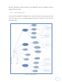
UML............................................................................................................................ 69
Evaluation ........................................................................................................................... 70
6.1
Program Code Testing................................................................................................ 70
6.1.1
Incremental testing ............................................................................................... 70
6.1.2
Class Tests.............................................................................................................. 70
6.1.3
General Tests for a different situations and selected options .............................. 71
6.1.3.1
Descriptive Statistics for one patient .......................................................... 72
6.1.3.2
Patients with different lengths of stay ........................................................ 72
6.1.3.3
Testing the analysis functionalities ............................................................. 72
8
6.1.3.4
Comparing Alive and Dead Patients ............................................................ 72
6.1.4
User test ................................................................................................................ 73
6.1.5
Tests with a large amount of data ......................................................................... 73
6.2
User Evaluations ........................................................................................................ 74
6.2.1
Analyst ................................................................................................................... 74
6.2.2
Preliminary clinician testing .................................................................................. 75
6.2.3
Statistical Feedback ............................................................................................... 77
6.2.4
Final clinician evaluation ....................................................................................... 79
7
Conclusions ......................................................................................................................... 80
8
Future Work........................................................................................................................ 81
8.1
Significant transitions points ..................................................................................... 81
8.2
Study the variability ................................................................................................... 81
8.3
Graphical information ................................................................................................ 81
8.4
Categorical variables .................................................................................................. 82
8.5
Checking assumptions ............................................................................................... 82
8.6
Automatic statistical test selection............................................................................ 82
8.7
Comparing days ......................................................................................................... 83
References................................................................................................................................... 84
General Bibliography ................................................................................................................... 86
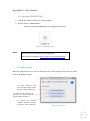
Appendix A. User Manual............................................................................................................ 87
A.1. Opening I-PREDICTOR ...................................................................................................... 87
A.2. Main screen ..................................................................................................................... 87
A.3. Consult or modify the field values ................................................................................... 88
A.3.1. Modify Hypothesis levels ......................................................................................... 89
A.3.2. Modify Medical Categories ...................................................................................... 90
A.3.3. Read file.................................................................................................................... 90
A.4. Consult, read or modify the Data Base ............................................................................ 91
A.4.1. Read the patient data............................................................................................... 92
9
A.4.2. Read the temporal data ........................................................................................... 92
A.5. Execute statistical functions ............................................................................................ 93
A.5.1. Select options ........................................................................................................... 93
A.5.2. Run the analysis........................................................................................................ 96
A.5.3. Results ...................................................................................................................... 96
A.6. Log file.............................................................................................................................. 97
Appendix B. Maintenance Manual .............................................................................................. 98
B.1. Dependencies .................................................................................................................. 98
B.2. Installing I-Predictor......................................................................................................... 98
B.3. Compile and build the system ......................................................................................... 98
B.4. Zip file .............................................................................................................................. 99
B.5. Source code ................................................................................................................... 100
B.5.1. In_Out package....................................................................................................... 100
B.5.2. Configuration package............................................................................................ 101
B.5.3. Data package .......................................................................................................... 101
B.5.4. Domain package ..................................................................................................... 102
B.5.5. Presentation package ............................................................................................. 103
B.5.6. Program package .................................................................................................... 104
B.6. UML Design .................................................................................................................... 105
B.7. System Configuration .................................................................................................... 107
B.8. Directions for future improvements .............................................................................. 109
B.9. Bugs and things to solve ................................................................................................ 112
Appendix C. Glossary of Terms.................................................................................................. 113
Appendix D. Tests Results ......................................................................................................... 114
D.1. TEST: Descriptive statistics for one patient ................................................................... 114
D.2. TEST: T-test .................................................................................................................... 117
D.3. TEST: Mann-Whitney U Test.......................................................................................... 118
D.4. TEST: Pearson correlation test ...................................................................................... 119
10
D.5. TEST: Patients with different lengths of stay ................................................................ 120
D.6. TEST: Comparing Alive and Dead Patients .................................................................... 121
Appendix E. Example of data set: Master File ........................................................................... 122
Appendix F. Example of data set: Slave File .............................................................................. 123
Appendix G. Use Cases Specification ........................................................................................ 124
Appendix H. UI Design ............................................................................................................... 135
Appendix I. Project Time Table ................................................................................................. 143
Appendix J. I–PREDICTOR Preliminary Evaluation .................................................................... 144
Appendix K. User test ................................................................................................................ 146
K.1. Definition ....................................................................................................................... 146
K.2. Template ........................................................................................................................ 147
K.3. Results 1 ......................................................................................................................... 152
K.4. Results 2 ......................................................................................................................... 157
Appendix L. “I PREDICTOR” versions ......................................................................................... 162
L.1. Version 1.0 ..................................................................................................................... 162
L.2. Version 2.0 ..................................................................................................................... 163
L.3. Version 3.0 ..................................................................................................................... 164
Appendix M. Statistical Research .............................................................................................. 165
M.1. Types of data ................................................................................................................ 165
M.2. Descriptive statistics ..................................................................................................... 167
M.2.1. A single variable .................................................................................................... 167
M.2.2. More than one variable......................................................................................... 170
M.3. Inferential statistics ...................................................................................................... 173
M.3.1. Sample selection ................................................................................................... 173
M.3.2. Normal distribution ............................................................................................... 173
M.3.3. Confidence intervals.............................................................................................. 175
M.3.4. Hypothesis testing ................................................................................................. 175
M.3.5. Correlation and regression.................................................................................... 181
11
Table of Figures
Figure 1 - Typical ICU Monitoring Equipment (1) ........................................................................ 17
Figure 2 - A-E Score(2) ................................................................................................................. 17
Figure 3 - Confusion Matrix for this domain (2) .......................................................................... 18
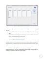
Figure 4 - SPSS viewer ................................................................................................................. 24
Figure 5 - SPSS data editor .......................................................................................................... 25
Figure 6 - Statgraphics application .............................................................................................. 25
Figure 7 - Use Cases Diagram ...................................................................................................... 39
Figure 8 - Non-functional requirements definition (11) ............................................................. 40
Figure 9 - Three Tier Architecture ............................................................................................... 43
Figure 10 – Controllers ................................................................................................................ 43
Figure 11 - Program flow ............................................................................................................. 44
Figure 12 – I-PREDICTOR Descriptive Statistics Tab (Statistical screen) ..................................... 47
Figure 13 - Hypothesis data example .......................................................................................... 48
Figure 14 - I-PREDICTOR: Correlation and Regression Tab (Statistical screen) ........................... 49
Figure 15 - I-PREDICTOR: Statistical tests Tab (Statistical screen) .............................................. 50
Figure 16 – I-PREDICTOR: Time Period Tab (Statistical screen), selecting days .......................... 50
Figure 17 - Comparing two natural days ..................................................................................... 51
Figure 18 - Comparing 24h period .............................................................................................. 51
Figure 19 - Whole stay for patients with different lengths ......................................................... 52
Figure 20 - I-PREDICTOR: Patients Tab (Statistical screen), selecting patients ........................... 52
Figure 21 - Time points during 24 hours ..................................................................................... 53
Figure 22 - Running averages over each hour (moving window = 4) .......................................... 53
Figure 23 - Running averages over each time point (moving window = 4)................................. 53
Figure 24 - Master and slave file ................................................................................................. 56
Figure 25 - I-PREDICTOR: Data Base screen, reading files........................................................... 57
Figure 26 - Example deducted missed value ............................................................................... 58
Figure 27 - Example of errors in the master file.......................................................................... 59
Figure 28 - Example of errors in the slave file ............................................................................. 59
Figure 29 - Read CSV process ...................................................................................................... 60
Figure 30 - Format Results .......................................................................................................... 64
Figure 31 - Netbeans Palette ....................................................................................................... 65
Figure 32 - I-PREDICTOR: main screen ........................................................................................ 65
12
Figure 33 - Navigation Map ......................................................................................................... 66
Figure 34 – Wait() (25) ................................................................................................................ 67
Figure 35 - Notify()(25) ................................................................................................................ 67
Figure 36 - Wait and Notify ......................................................................................................... 68
Figure 37 - System UML .............................................................................................................. 69
Figure 38 - Netbeans: Program structure ................................................................................... 70
Figure 39 - Tests data package .................................................................................................... 71
Figure 40 - Tests In_Out package ................................................................................................ 71
Figure 41 - Tests domain package ............................................................................................... 71
Figure 42 - I_PREDICTOR.jar file .................................................................................................. 87
Figure 43 - Main screen ............................................................................................................... 87
Figure 44 - Manage field values screen ....................................................................................... 88
Figure 45 - Modify hypothesis levels screen ............................................................................... 89
Figure 46 - Modify medical categories screen ............................................................................ 90
Figure 47 - Example of the CSV field file ..................................................................................... 90
Figure 48 - Data Base screen ....................................................................................................... 91
Figure 49 - Data Base read .......................................................................................................... 91
Figure 50 - Execute statistical functions screen .......................................................................... 93
Figure 51 - Select time period ..................................................................................................... 93
Figure 53 – Select statistical tests ............................................................................................... 94
Figure 52 - Select descriptive statistic ......................................................................................... 94
Figure 54 - Select correlation and regression ............................................................................. 95
Figure 55 – Information about the elected options .................................................................... 96
Figure 56 - Analysis Results ......................................................................................................... 96
Figure 57 - Log file ....................................................................................................................... 97
Figure 58 - Ctrl_Program UML .................................................................................................. 105
Figure 59 - UML Data Tier ......................................................................................................... 105
Figure 60 - UML Domain Tier .................................................................................................... 106
Figure 61 - Presentation UML ................................................................................................... 106
Figure 62 - System UML ............................................................................................................ 107
Figure 63 - Adding statistical options ........................................................................................ 109
Figure 64 - Test results (1.1) ...................................................................................................... 115
Figure 65 - Test results (1.2) ...................................................................................................... 116
Figure 66 - Test results (1.3) ...................................................................................................... 116
Figure 67 - Results t-Test ........................................................................................................... 117
13
Figure 68 - Results Mann-Whitney Test .................................................................................... 118
Figure 69 - Results Pearson Test ............................................................................................... 119
Figure 70 - Mean for different patients .................................................................................... 120
Figure 71 - Comparing Alive and Dead Patients ........................................................................ 121
Figure 72 - Example of data set: Master File ............................................................................. 122
Figure 73 - Example of data set: Slave File ................................................................................ 123
Figure 74 - Volere requirements template ............................................................................... 124
Figure 75 - I-PREDICTOR timetable ........................................................................................... 143
Figure 76 - Example of temporal data ....................................................................................... 166
Figure 77 - Bar chart .................................................................................................................. 167
Figure 78 - Pie chart .................................................................................................................. 167
Figure 79 - Stacked bar chart .................................................................................................... 170
Figure 80 - Grouped bar chart ................................................................................................... 170
Figure 81 - Box plots .................................................................................................................. 170
Figure 82 - Linear relationship .................................................................................................. 171
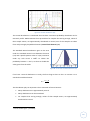
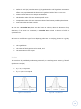
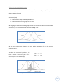
Figure 83 - Normal distributions (30) ........................................................................................ 174
Figure 84 - Area under normal distribution (31) ....................................................................... 174
Figure 85 - Confidence intervals (32) ........................................................................................ 175
Figure 86 - One sided test ......................................................................................................... 176
Figure 87 - Two sided test ......................................................................................................... 176
Figure 88 - Diagram to choose an appropiate test statistic (15) ............................................... 177
Figure 89 - Comparison of the means for two populations(29)................................................ 179
Figure 90 - Comparison of means, One side test ...................................................................... 179
Figure 91 - Simple Linear Regression (15) ................................................................................. 182
14
Table of Tables
Table 1 - Input data types ........................................................................................................... 31
Table 2 – Risk: Delivery date ....................................................................................................... 33
Table 3 – Risk: Speed ................................................................................................................... 33
Table 4 – Risk: Large data base ................................................................................................... 34
Table 5 – Risk: Incompatibility with the client’s computer ......................................................... 34
Table 6 – Risk: Incompatibility with the Java Statistical Library.................................................. 35
Table 7 – Risk: No time to make a good UI ................................................................................. 35
Table 8 – Risk: User requirements .............................................................................................. 36
Table 9 – Risk: Lack of information ............................................................................................. 36
Table 10 - User: Clinician ............................................................................................................. 37
Table 11 - User: Analyst............................................................................................................... 37
Table 12 - Summary of use cases ................................................................................................ 40
Table 13 - System tasks ............................................................................................................... 45
Table 14 - Descriptive functions for the project data ................................................................. 48
Table 15 - Hypothesis Codification.............................................................................................. 48
Table 16 – Example of running averages .................................................................................... 49
Table 17 - Comparing two natural days ...................................................................................... 51
Table 18 - Comparing 24h time period ....................................................................................... 51
Table 19 – Whole stay for patients with different lengths ......................................................... 52
Table 20 - Comparasion between statistical Java libraries ......................................................... 62
Table 21 - Suggestions analyst evaluation .................................................................................. 75
Table 22 - Tasks realized at the second evaluation..................................................................... 76
Table 23 – Clinicians’ suggestions, first evaluation ..................................................................... 77
Table 24 – Statistician’s suggestions ........................................................................................... 78
Table 25 – Clinicians’ suggestions, second evaluation ................................................................ 79
Table 26 - Netbeans: Open project ............................................................................................. 98
Table 27 - Zip folders ................................................................................................................... 99
Table 28 - I-PREDICTOR packages ............................................................................................. 100
Table 29 - In_Out package......................................................................................................... 101
Table 30 - Configuration package.............................................................................................. 101
Table 31 - Data package ............................................................................................................ 102
Table 32 - Domain package ....................................................................................................... 102
15
Table 33 - Presentation package ............................................................................................... 103
Table 34 - Program package ...................................................................................................... 104
Table 35 - Patient 2121 data ..................................................................................................... 114
Table 36 - Patient 2121 temporal data ..................................................................................... 114
Table 37 - Steps results ............................................................................................................. 151
Table 38 - Steps results ............................................................................................................. 156
Table 39 - Steps results ............................................................................................................. 161
Table 40 - I PREDICTOR v1.0 ...................................................................................................... 162
Table 41 – I PREDICTOR v2.0 ..................................................................................................... 163
Table 42 - I PREDICTOR v3.0 ...................................................................................................... 164
Table 43 - Statistical types of data ............................................................................................ 165
Table 44 – Frequencies.............................................................................................................. 167
Table 45 - Cumulative percentages ........................................................................................... 167
Table 46 - Different distributions .............................................................................................. 169
Table 47 - Contingency table..................................................................................................... 170
Table 48 - Types errors .............................................................................................................. 177
16
1 Introduction
1.1 Overview
The Intensive Care Unit (ICU) at
Glasgow Royal Infirmary is a section
within the hospital which looks after
patients who are critically ill, or
unstable,
and
require
intensive
treatment and monitoring to help
restore
them
to
more
normal
physiological ranges. Examples of
conditions encountered in an ICU are:
Heart
surgical
attack,
stroke,
complications,
pneumonia,
burns
or
Figure 1 - Typical ICU Monitoring Equipment (1)
various traumatic incidences. About
350 patients a year are admitted at ICU at Glasgow Royal Infirmary, with an average stay 7
days. However, a big difference exists between the average stay in the ICU at Glasgow Royal
Infirmary and the rest of Scottish ICUs (1).
INSIGHT is a tool which supports domain experts exploring, and removing, inconsistencies in
their conceptualization of a task. INSIGHT allows a domain expert to compare two perspectives
of a classification task. The ICU at Glasgow Royal Infirmary has developed a 5-point scoring
schema: A to E (A means that the patient is ready to be discharged and E means that the
patient is extremely ill) (2).
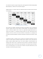
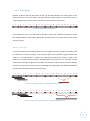
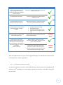
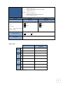
E
D
C
B
A
Patient is highly unstable with say a number of his physiological parameters (e.g., blood
pressure, heart rate) having extreme values (either low or high).
Patient more stable than patients in category E but is likely to be receiving considerable
amounts of support (e.g., fluid boluses, drugs such as Adrenaline, & possible high doses of
oxygen).
Either more stable than patients in category D or the same level of stability but on lower
levels of support (e.g., fluids, drugs & inspired oxygen)
Relatively stable (i.e., near normal physiological parameters) with low levels of support.
Normal physiological parameters without use of drugs like Adrenaline, only small amounts of
fluids, and low doses of inspired oxygen.
Figure 2 - A-E Score(2)
17
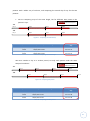
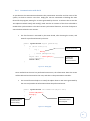
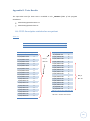
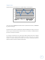
One example of a patient’s progress during hourly reporting periods would be: E, E, D, E, D, D,
D, C, D, C, D, C, C,... Where we can see a positive progress.
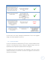
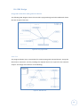
INSIGHT displays in a confusion matrix the information about the instances which have been
misclassified (2).
Figure 3 - Confusion Matrix for this domain (2)
Score systems are needed to determine the severity of the patients. They can provide the
clinicians a regular summary of each patient’s overall condition. Such information would be
useful to determine whether there has been any appreciable progress/deterioration (2).
Another score, Apache II, is created once during a patient’s ICU stay, usually 24 hours after
admission, but does not take into account the effect of interventions on a patient(2). The
information produced by INSIGHT is collected at specified time periods and recorded in a data
base.
An additional program is needed to help to analyse the information produced by the ICU’s
systems: A-E Score, patient’s predicted mortality and the Apache II scores; jointly with the
patient's medical condition (Sepsis, Burns, etc.) and the patients’ outcome (patient's ICU
discharge status: dead or alive). In particularly the ICU clinicians are interested in analyse the
relation between patient scores and their other parameters. The required system will make it
easy for clinicians/analysts to run these sorts of studies. The system should be easy to be
extended to include further types of analyses.
18
1.2 Motivation
1.2.1
Why do the clients need a new program?
The clinicians and the analysts of Glasgow Royal Infirmary’s ICU want to do statistical studies of
their patients using the available information. There are many existing statistical programs that
could be used for this purpose (for example, SPSS1), so why do they need a new program?
Most of the existing statistical programs are general purpose and hence they are complex to
use. We must bear in mind that the clinicians aren’t experts in informatics or statistics, and
some of them may have problems in working with a computer. So, how can they work with a
program having many features? What statistical methods should they choose?
Another factor that we must bear in mind is that these programs require specific input data
formats and if we want to use them, we must adapt our data to the required format. The ICU
of Glasgow Royal Infirmary has the patient data in a format produced by their systems. So
what if these data are not in the appropriate input format for the statistical programs?
Transforming the data to a specific format takes time and needs to be done every time we are
going to do a study with a different dataset.
1.2.2
My project
The objective of my project is to solve these problems with a new computer program which is
able to read the data in the format used by the INSIGHT system, is intuitive and is easy for the
clinicians to use. The program has been created to help the target audience to achieve specific
objectives, and provides the necessary statistical tools.
1
See section 3.1.1 (SPSS)
19
1.3 Objectives
1.3.1
Clinicians’ objectives
The clinicians have specific types of clinical research questions that they would like answered
by the tool. The clinicians’ objectives include the following:

Determine the earliest time in all patients’ stays at which it would be possible to find a
significant discrimination between patients who leave the ICU alive and those who die.

Determine for each patient the significant transition points for one of its parameters
(e.g. A-E Score1), when it changes value from one category to another, and remains
stable at the new category for a period of time.
However, the above objectives are defined in general terms, so we need specific objectives for
our statistical program, to define what it’s going to do. We have identified a number of
primary goals and these should be covered by the end of the project. Additionally, we have
some secondary goals, the optional points for the project. These secondary goals will be
addressed if there is time.
1.3.2
Primary goals
(a) Read and store the data of the patients in the original format.
(b) Provide a tool to calculate the averages of the temporal data, for various time intervals
and for selected patients.
(c) Provide a tool to study the discrimination between the two groups of patients (Dead
and Alive upon leaving the ICU). The tool should examine different time periods,
parameters, and medical categories.
(d) Provide a tool to study the relation between the different physiological parameters of
the patients for each of the different medical categories.
(e) Create a report with the results of the study.
(f) Provide an interface for the user.
1
See Figure 2 - A-E Score.
20
1.3.3
Secondary goals
(g) Ability to exclude an initial period of H hours for all the patients when calculating the
average of the temporal data.
(h) Ability to exclude certain patients from the analysis.
(i) Ability to analyze the last N days of each patient’s records.
(j) Ability to present the results graphically.
(k) Provide a tool to report the running averages of the temporal data and to have the
ability to define the size of the moving window, for a various time intervals and for
each patient.
(l) Report the important transition points of the running averages, where the analyst
should be able to specify the threshold of interest and the number of time points that
the value has to remain stable to be significant.
(m) Provide a tool to report the number of records associated with each patient.
(n) Report descriptive information for each of the main diagnostic categories.
21
2 Background
2.1 Statistical background
2.1.1
Biostatistics
Statistics deals with the methods and procedures for collecting, classifying, summarizing and
analyzing data; as well as making inferences in order to make predictions and to assist
decision-making. Therefore we could classify Statistics as descriptive, when results of the
analysis are not beyond the dataset and as inferential statistics when the objective of the study
is to extrapolate the conclusions reached about the sample to the population.

Descriptive statistics: Describes, analyzes, and represents a group of data using
numerical and graphical methods to summarize and present the information
contained therein.

Inferential statistics: Based on the calculation of probabilities and based on sample
data, makes estimates, decisions, predictions, or other generalizations about larger
population.
Biostatistics is a branch of statistics, sometimes considered to be a branch of medical
informatics, which deals with problems in life sciences such as biology, medicine, etc. Some of
the applications of biostatistics are (3):

In medicine and epidemiology, the design and analysis of different types of study, for
example, clinical trials (to evaluate interventions) or cohort studies (studying the
natural history of disease and the factors that determine it).

In public health, to describe the health of the population or to assess the impact of
intervention programs.

In biology, to relate the characteristics of the phenotype with the genotype.

In order to improve agricultural crops and livestock.
Biostatistics has become one of the basic sciences of medicine. This is mainly due to doctors’
requirements, for example, to predict whether a patient might be cured by a given treatment.
22
They also want to know how the disease will develop. These predictions are only possible using
the tools of biostatistics.
2.1.2
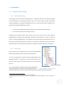
Performing statistical studies
When we perform a statistical study, we have to carry out a given process in order to achieve
the desired results (4):

What do we want to study?

Decide what data has to be collected (variables), from what population and how to
select the sample to be used for the study.

Collect the data.

Analyze the collected data.

Study the resulting information data and draw conclusions.
2.1.3
Statistical Research
A large part of my project is to implement statistical functions. Before start designing and
implementing the system to perform and statistical study, an extensive research for the
different parts of statistics relevant for my program has been done. This information has been
used to make design decisions. This research can be found in Appendix M.
2.2 Similar systems
In addition to reviewing the statistical background in this report, we need to recognize the
existing statistical programs on the market. These programs will be discussed further in the
next section, since they must be analyzed before proceeding with the design of the
application.
We can find a lot of statistical programs to download from the Internet. Since it is impossible
to study and analyze each one of them, we are going to study some of the more important
ones that are used commercially:

IBM SPSS Statistics

Statgraphics

Microsoft Excel
23
3 Analysis
3.1 Evaluation of similar systems
If there are existing statistical programs on the market, why not use them?
What problem does the client have with them?
What are the important differences between existing programs and the program we are
designing?
To answer these questions, we have to analyze the different existing statistical programs. In
this analysis we can study and appreciate the complexity of these programs and also extract
some ideas for our system.
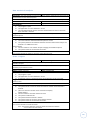
3.1.1
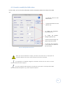
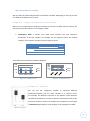
SPSS
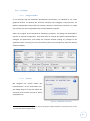
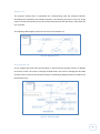
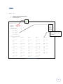
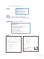
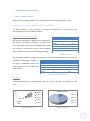
Statistical Package for the Social Sciences (5) (by SPSS Inc.) is a very popular statistical
program used in many studies and different companies. The program has all the functionalities
to report Descriptive Statistics, Bivariate Statistics and Predictions, and has the capability to
present the information graphically and to work with sizeable data bases. It offers various
modules for the different types of functions that can be purchased separately.
The program can deal with
several different data files
(including Excel and Lotus
spreadsheets, and database
tables
from
various
sources). Version 14.0 has
eight different windows to
process
the
data
display
the
results
and
of
studies, and each of these
windows has its own menu
(See Figure 4 and Figure 5).
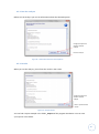
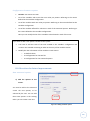
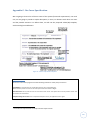
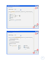
Figure 4 - SPSS viewer
24
In
fact,
SPSS
is
very
complete and capable of
performing
all
the
calculations and statistical
analysis that we need. We
can get an idea of its
functionality by consulting
the user manual (for the
version 14.0) which has
more than 800 pages (6).
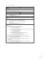
Figure 5 - SPSS data editor
3.1.2
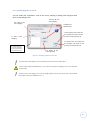
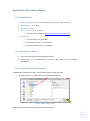
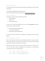
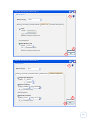
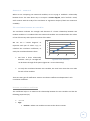
Statgraphics
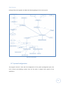
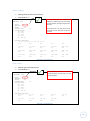
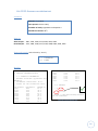
Another available statistical program is STATGRAPHICS (7) (by StatPoint Technologies, Inc.).
There is an online version (8), which performs some calculations, but this version has
restrictions concerning the size of files.
Figure 6 - Statgraphics application
25
This program can read several different formats for input data, but although it has fewer
functionalities than SPSS, it is still complicated to use. Statgraphics basic functionalities are:
analysis of variance, basic graphics development, categorical data analysis, comparison of two
or more samples, descriptive methods, experimental designs, life data analysis, multivariate
methods, regression analysis, statistical process control and time series analysis. Knowing that
it has a manual of 300 pages, and looking at the program’s features (Figure 6), we can gain a
sense of its complexity.
3.1.3
Microsoft Excel
Another existing program that we can consider when we want to do a statistical study is
Microsoft Excel. It seems to be an appropriate program if the data is provided in a worksheet.
However, Excel is not a simple program to use, much less so if we are conducting a complex
statistical study in which we want to change the input data easily, and which takes different
time periods into account. In considering Excel it is important to be aware that it is not a
statistical program, but rather a data analyses system. It has less than a quarter of the
statistical functionalities of the other programs mentioned above and so it is limited to the
basic ones. What it does have is the ability to generate many types of graphical reports,
although some of them would require the user to consult the manual to enter the data
correctly.
3.1.4
Conclusions
We could use an existing statistical program to do the required analysis, as they contain all the
functionality needed. But with a general statistical program, the user must know what data to
select, and how to select it, for each of the statistical functions to be applied. A person familiar
with the computer and statistical procedures may be able to use existing systems without any
problem, but may have to devote some time to adapting the data. But a person unaccustomed
to working with computers or a person with little statistical knowledge may need to study
statistical theory and large program manuals. This is not appropriate for this particular
problem domain.
A further program with these tools is data preparation. In the ICU domain, large volumes of
data are produced by patient monitoring equipment. Adapting data to work with these
statistical packages would be extremely time consuming and not practical.
26
3.2 Project purpose
3.2.1
The users’ requirements
The first thing we have to analyze is the users’ requirements, in order that the program can be
appropriate for the users’ needs. As we have discussed above, the clinicians find it difficult to
use the existing statistical programs, which are complex and have too many features. In
addition to having problems using the current statistical programs, the clinicians wish to avoid
transforming the collected data into another format. We have a particular type of data
(temporal data1), which needs to be handled in specific ways defined by the clinicians.
The client wants a computer program for processing their patient data in a particular format.
This program should be intuitive and easy to use, and should have a number of statistical
functions focused on the objectives set out below.
3.2.2
Analysis of objectives
Finally, we have to analyze the objectives of the (statistical) analyses that the client wants to
perform. It is very important to have defined objectives from the beginning, to avoid the
possibility of the project being misdirected. We have previously defined two objectives2:

Determine the earliest time in all patients’ stays at which it would be possible to find a
significant discrimination between patients who leave the ICU alive and those who die.

Determine for each patient the significant transition points for one of its parameters
(e.g. A-E Score), when it changes value from one category to another, and remains
stable at the new category for a period of time.
1
2
See chapter 3.4.2. (Second file)
See chapter 1.3.1. (Clinicians’ objectives)
27
3.3 Constraints
3.3.1
Environment
We must be aware that the program should be able to be used on the hospital and analysts’
computers. So, when we are developing it we have to be sure that it works properly on the
following operating systems and versions: Windows XP, Windows Vista, and Windows 7.
3.3.2
Project planning
The project time schedule shall be adjusted to the time frame defined by the department of
Computing Science of the University of Aberdeen for the project (12 weeks). We must be
realistic when we are specifying the functionalities of the program, in order that we have
enough time to complete the development and evaluation of the system. To organize it, it is
necessary to make a project plan which is appropriately scheduled. We need to plan all tasks,
their sequencing and the estimated time for each one. The timetable made for "I PREDICTOR"
can be found in Appendix I.
3.3.3
Economic restrictions
Another thing to bear in mind is that we have no budget to develop the program. That is, any
application or external tool to be attached or used in our project, must be available free of
charge.
28
3.4 Input data
One of the things that we must analyze is the nature of the datasets to be processed. This is
important for designing their input to the system and the way that they will be saved. It also
provides information about which statistical functions should be applied to achieve the desired
results. The population for this study comprises patients of the ICU at Glasgow Royal Infirmary.
The data has been collected anonymously, according to the requirements of the Data
Protection Act 1998 (9), from a sample of patients, for each medical category to be studied.
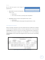
The data are provided in two CSV files. The first file contains the static data for each patient,
that is to say, only those variables that have only one value per patient (e.g. patient’s medical
category). The second file contains the temporal data of the patients, that is, those variables
whose value changes over time (e.g. patient’s severity score).
3.4.1
First file1
To begin, we will analyze the file containing the static data.
It comprises, N lines
corresponding to N different patients, and has six columns (but only five of them are of
interest to us):

Patient-ID: represents the identifier of the patient.

Outcome: indicates the patient's ICU discharge status and can take the values Dead or
Alive.

Apache II: this variable determines a score, based on the Apache scale [16], which is a
range of integers from 0 to 71.

Predicted Mortality: this is a percentage value derived from the patient’s Apache II
score and the patient’s medical category.

1
Medical Diagnostic: indicates the patient's medical status.
We can find an example of this input file in Appendix E.
29
3.4.2
Second file1
As previously stated, the second file contains the temporal data of the patients. This file will
have as many lines of temporal data per patient as the number of occasions that temporal
data have been collected for him, and the data for each patient is in time sequence and
appears together in the file. The file has three columns of interest to our study:

Patient-ID: represents the identifier of the patient and appears only on the first line of
the patient.

Time of Time point: indicates the date and time at which the value was collected.

Hypothesis2: The ICU at Glasgow Royal Infirmary has developed a five-point scoring
schema (A means that the patient is ready to be discharged and E means that the
patient is extremely ill). The values of this variable can be: A, B, C, D, E. This will be the
default scale in our study, but could be modified in further studies.
3.4.3
Comments about the input data
Initially, the input data consisted of only one input file containing all patient data, and also
contained one attribute less for each patient. The real format of the data (two files and a new
field), was not presented to me until the first week of December (10th week of my project),
when the reading data, the database and the program interface were already completed.
This change led to me modify the reading of the CSV files, to be able to read the separate
information and modify the data base by adding a new variable for the patients. I also had to
modify the interface of the program, to be able to select the two types of file and extend the
respective screens to add the new variable.
1
We can find an example of this input file in Appendix F.
2
The variable Hypothesis refers to the A-E Score. See Figure 2 - A-E Score.
30
3.4.4
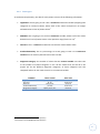
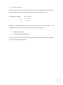
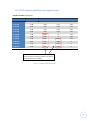
Data types
As we discussed previously, the data for each patient consists of the following information:

Hypothesis: we are going to use it like a continuous numerical variable (mapping their
categories to numerical values), where each of the values correspond to an integer
and determines a level of patient status1.

APACHE II: we are going to use it like a continuous variable, where each of the values
determines a level of patient status in the Apache II range (from 0 to 71)2.

Outcome: This is a nominal variable that can take the values Dead or Alive.

Predicted Mortality: This is a percentage, so we are going to treat it as a continuous
variable that can take any decimal value from 0 to 100.

Diagnostic Category: The number of values that this nominal variable can take is the
as the number of medical categories in use. All the studies that we will do in the
project are for the different diagnostic categories, so these categories won’t be
compared and we do not need to treat it as a numerical variable.
VARIABLE
Hypothesis
Apache II
Outcome
Predicted Mortality
Diagnostic Category
INPUT VALUES
A, B, C, D, E (1,2,3,4,5)
[0..71]
Dead, Alive
[0..100]
Sepsis, Burns, etc.
DATA TYPE
Continuous
Continuous
Nominal
Continuous
Nominal
Table 1 - Input data types
1
2
See section 5.3.1 (I-PREDICTOR assumptions).
See section 5.3.1 (I-PREDICTOR assumptions).
31
3.5 Risk management
During the development of any project, there may be external factors that can impact on
objectives to a greater or lesser degree. We can encounter two different types of risks:
Negative risks and Positive risks.
It is an important to define the means by which we can manage the negative risks. We could
apply three different methods (10):

Avoid: Plan the project in such a way that it would not be affected.

Mitigate: Identify ways to minimize either the likelihood or the affect of the risk.

Transfer: Organize the project to divert the risk.
For the positive risks, we could apply three different methods (10):

Exploit: Plan the project in such a way that the risk would occur.

Enhance: Identify ways to maximize either the likelihood or the affect of the
opportunity.

Share: Identify a third party who is better placed to utilize the opportunity on behalf of
the project.
It’s necessary to identify the assumed risks and to define them and their contingency plan
correctly. In our project, the assumed risks are the following:
32
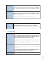
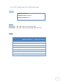
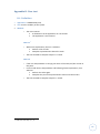
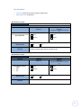
3.5.1
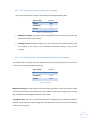
The system may not be ready for the agreed date
It may not be possible to have the system ready for the agreed delivery date.
Type of Risk
Internal
Impact
High
Probability
5%
Priority
1
Table 2 – Risk: Delivery date

Mitigation Strategy: the project will be well planned with reference to the tasks and
the time devoted to each of them.

Contingency Plan: Identify in advance any minor features that could be omitted from
the program in the event of any unforeseen eventuality causing a delay to the
schedule.
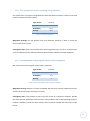
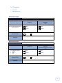
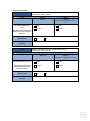
3.5.2
The system speed is reduced when dealing with a large database
The system works too slowly when the data base has more than 150 patients with a mean of
170 time points of temporal data per patient.
Type of Risk
Internal
Impact
Medium
Probability
25 %
Priority
0.25
Table 3 – Risk: Speed
Mitigation Strategy: we will perform tests with various quantities of data to check the speed
of the system. However, the preference for the system is to work with a large amount of data,
but sometimes this could affect the speed of the system.
Contingency Plan: We can try to perform the analysis separately for the different statistical
options and the different medical categories. We could also increase the amount of memory
available to the program.
33
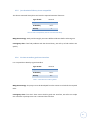
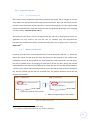
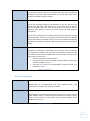
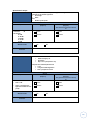
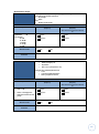
3.5.3
The system freezes when analyzing a large database
The system does not support a large date base with 150 patients and with a mean of 170 time
points of temporal data per patient.
Type of Risk
Internal
Impact
Medium
Probability
Priority
15 %
0.7
Table 4 – Risk: Large data base
Mitigation Strategy: we will perform tests with different amounts of data to check the
functionality of the system.
Contingency Plan: If the system breaks down with a large data base, we can try to perform the
analysis separately for the different statistical options and the different medical categories.
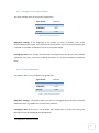
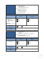
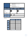
3.5.4
Incompatibility of the program with the client’s computers
We cannot execute the program on the client’s machines.
Type of Risk
External
Impact
Low
Probability
5%
Priority
1
Table 5 – Risk: Incompatibility with the client’s computer
Mitigation Strategy: develop a system compatible with the most common operating systems,
and be sure that the client is using one of them.
Contingency Plan: If the problem is due to the Java version on a particular computer, provide
the client with the appropriate version of Java. If the problem is due to the operating system or
hardware available, provide the client with the list of resources needed and where they can be
found.
34
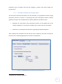
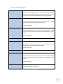
3.5.5
Java Statistical Library is not compatible
The chosen statistical library does not have the required statistical functions.
Type of Risk
Internal
Impact
Medium
Probability
30 %
Priority
1
Table 6 – Risk: Incompatibility with the Java Statistical Library
Mitigation Strategy: Study and thoroughly test some different libraries before selecting one.
Contingency Plan: If we find problems with the chosen library, we will try to find another one
quickly.
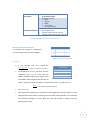
3.5.6
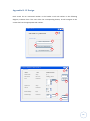
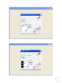
No time to make a good user interface
It is not possible to develop a good interface.
Type of Risk
Internal
Impact
Low
Probability
50 %
Priority
0.1
Table 7 – Risk: No time to make a good UI
Mitigation Strategy: The project must be developed from the outset to include all the required
tasks.
Contingency Plan: If we don't have time to build a good user interface, we will use a simple
user interface or perhaps even use a command line interface.
35
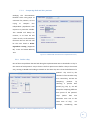
3.5.7
Changes in user requirements
The client changes some of the system requirements.
Type of Risk
External
Impact
High
Probability
30 %
Priority
0.75
Table 8 – Risk: User requirements
Mitigation Strategy: at the beginning of the project, we have to develop a list of the
functionalities of the system. If the client wants a feature that was not previously defined, this
is treated as a possible modification, but not as a required change.
Contingency Plan: If the changes are discussed at the beginning of the project, they could be
considered, but if they arise in the middle of the project, it may not be possible to implement
them.
3.5.8
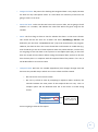
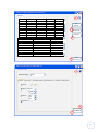
Lack of information
The patients’ data is not provided by the agreed date.
Type of Risk
External
Impact
High
Probability
70 %
Priority
0.75
Table 9 – Risk: Lack of information
Mitigation Strategy: The patient data from the ICU at Glasgow Royal Infirmary should be
obtained as early as possible so as to avoid such problems.
Contingency Plan: If the data is not provided with enough time to realize the testing, the
planned tests will be developed with pseudo data1.
1
See Appendix C. Glossary of Terms.
36
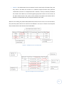
4 Requirements
4.1 Product users
The clients are a very important aspect of our system, because the purpose of our project is
that the system will be finally used by them. When we have more than one user, we have to
bear in mind that they may have different knowledge and different experience concerning the
problem. This means taking many decisions while we are designing the program. In our case
we have two different types of users to analyze:
User Name
Clinician
Role
Final user of the software
Technology experience
Low
Statistical experience
Low
Table 10 - User: Clinician
User Name
Analyst
Role
Final user of the software
Technology experience
Statistical experience
High
Medium
Table 11 - User: Analyst
4.2 Functional requirements
4.2.1
What the system does
After the analysis of user requirements, the existing statistical programs and the data that the
system has to analyze, we have to define the functionalities of the system.
The first important functionality is to read the patient data to perform a statistical analysis. As
previously discussed, this information is separated into two different CSV files, one with the
static information for each patient, and the other one with the temporal data for each patient.
So, the user has to be able to manage the data base, with these actions:
37

Read the static patient data

Read the temporal data

Delete the data base (to be able to read different data files in the same execution).
Another thing we have to consider is that the values of the data base have to be correct and
the system has to check it by reading the files. However, the user could want to modify the
restrictions for some of these values in later studies, so we have to consider the functionality
for managing the field values. The field values that the user has to be able to modify are the
hypothesis levels and the list of medical categories. To make the functionality useful, the user
should be able to:

Restore the default values.

Modify the values of the hypothesis and medical category manually.

Read the new values for the hypothesis and medical category from a CSV file.
The most important functionality of the application is the performance of statistical analysis.
The user has to be able to select the medical category, the patients, and the time period for
the study. We consider the time period as a range of days, with the possibility to exclude an
initial period of N hours. Referring to the statistical functions that can be realized, three
important groups should be available: Descriptive Statistics, Statistical Tests to compare the
selected Dead and Alive patients, Correlation and Regression to compare two variables of the
selected patients. The user has to be able to select the confidence intervals1 and the variables
to study.
The application has to check the selected options for the study, to inform the user about
possible things to consider before running the analysis. Additionally, the application has
provide the user the option to print the results in a file. So the user will be able to:

Select the options and the data for the analysis.

Check the selected options.

Run the analysis.

Print the results.
1
See section M.3.3. Confidence intervals (Appendix M).
38
We must remember the basic functions of the application: open the program, close the
program and consult help.
4.2.2
Users and Use Cases
The system functionalities are basically the use cases of the system. They interact with each
other and with the user. The following diagram shows the existing use cases and their
interrelationships:
Figure 7 - Use Cases Diagram
39
The specification of each use case is in Appendix G. For each one there is a simple description,
its actor, its relationships with other use cases and possible scenarios.
1
2
3
4
5
6
7
8
9
10
11
12
13
14
15
16
17
Open program
Close program
Consult help
Manage field values
Restore default field values
Read the new values from a file
Modify medical categories
Modify hypothesis levels
Manage data base
Clear data base
Read patients data
Read temporal data
Execute statistical analysis
Select the data and the options
Check selected options
Run statistical analysis
Print a report
Table 12 - Summary of use cases
4.3 Non-functional requirements
Non-functional requirements are the properties that the functions must have, such as
performance and usability. These requirements are as important as the functional
requirements for the product's success.
Figure 8 - Non-functional requirements definition (11)
4.3.1
Appearance

A very important aspect of a program is that the style of all screens is consistent.

The system should be user friendly, so that the user can move easily through the
screens. In order that the users can offer their opinions, we will present them with a
preliminary design of the system.
40
4.3.2
Usability

The program should be simple and intuitive to use.

The user will not need any previous information to move through the system.

In each screen the user will be offered a help tool for any problem.

Since the program is designed for the ICU of the Glasgow Royal Infirmary, the language
of the interface and all related documentation will be in English.

The system must help the user avoid mistakes in entering the data.

The decimal numbers will be represented with a point. Example: 9.10.

All presented non-integer data will be rounded to two decimal places.
4.3.3

Performance
The system should support at least 15 patients with a mean of 100 time points of
temporal data.

The system should carry out the statistical calculations in a maximum of 5 seconds.
4.3.4

Environment
The system should be compatible with any computer that supports java and with the
operating system: Windows XP, Windows Vista and Windows 7.
4.3.5
Support and maintenance

The system should be expandable.

The system, should not have unexpected errors, but if an error occurs, the system
should recover appropriately (whenever possible).
4.3.6

Security
The system should check the data entered by the user, because incorrect data will lead
to incorrect and unexpected results.
4.3.7

Legal
The patient data provided by the Glasgow Royal Infirmary must not violate the Data
Protection Act 1998(9).
41
5 Design and Implementation
5.1 Application Language
5.1.1
Why JAVA?(12)
Java is an object-oriented language and there are a number of reasons for deciding to use Java
to implement a computer program:

It is a distributed language.

It is an interpreted language: this slows the program, but gives flexibility.

It is a robust and reliable language.

It is an important tool for developing distributed applications because it is a
multiplatform language (portable).

A program developed with Java does not need to be compiled again to be executed on
any platform with the corresponding JRE version installed.

Offers a big reutilization of code, with the possibility of finding many free libraries.

High performance.

It is concurrent (allows the execution of multiple threads).

It is a simple language, without using pointers or the manipulation of memory.
5.1.2
Java Version
The Java version used to develop the application is the version: 1.6.0_20. To be able to run the
program on another computer, it has to have Java version 1.6.
5.2 Architecture
5.2.1
Tiers architecture
When designing a system and its components, it is a good practice to use design patterns. Each
design pattern has specific characteristics and objectives. The design pattern based on tiers (or
layers), has the advantage that it makes exchangeability easy, is easy to extend, can be
maintained with relative ease and can be restructured. However, it can lead to redundant
coding (13).
42
An architecture based on tiers has the following properties:

The components of the system are grouped by tiers.

The communication is only allowed between elements of the same tier or contiguous tiers.
The most common architecture is the well-known Three-Tier architecture which is designed as
follows:
Presentation Tier
Responsible for displaying the data to the user, but ignores the internal
working of the system.
Domain Tier
Responsible for meeting the requests of the user, but ignores how the
data are stored and how they are presented to the user.
Data Tier
Knows how data is stored in the system, but ignores how the data will
be treated or how they will be presented to the user.
Data Base Management System
Figure 9 - Three Tier Architecture
With this structure we can achieve the objective of only affecting the corresponding layer
when possible changes occur in the representation of the data, in the interface, etc...
5.2.2
Tiers Controllers
Our system will be based on the
PROGRAM
CONTROLLER
architecture described previously
but with some additional features.
Sometimes we need a class to
group
the
other
ones
and
coordinate their functionalities.
DATA
CONTROLLER
DOMAIN
CONTROLLER
PRESENTATION
CONTROLLER
These classes are called the
Figure 10 – Controllers
43
Controllers. These controllers will help us to organize the logic of the program and to enable
communication between the tiers. We are going to use one controller for each tier, and an
additional one responsible for maintaining the flow of the program and to coordinate the
other controllers. The different tiers will not communicate directly, they will communicate
with the rest of the system through the general controller and the corresponding tier
controller1.
5.2.3
Tiers communication and program controller
To communicate between the different layers of the system, we have a general controller,
called the program controller, which contains instances of the other controllers enabling
communication to be established between them.
The main function of this controller is responsible for carrying out the flow of the program.
This flow is controlled by a loop which, in each execution, performs a task and collects the next
task to be carried out.
The following box shows the scheme to control the flow of the program:
task = Execute Main Screen
while(true){
switch(task){
case 1:
EXECUTE TASK 1
task = new task
break;
case 2:
EXECUTE TASK 2
task = new task
break;
.....
case N:
EXECUTE TASK N
task = new task
break;
}
}
Figure 11 - Program flow
1
Tiers and controllers design: See section B.6. (Appendix B) for more information.
44

Each of the tasks will be performed by a particular controller.

For tasks carried out by the Data controller, the Domain controller and the Program
controller, the next task is specified and is always the same (e.g. After reading the
temporal data file, the data will be displayed on the Data Base screen).

However, for most of the tasks realized by the Presentation controller, the next task to
be executed will be defined by the user (e.g. After displaying the Data Base screen the
user can choose to return to the main screen, clear the data base, read the file with
the patient data or read the temporal data file.)
The following table shows all tasks that can be performed by the program, along with their
responsible controllers and succeeding tasks.
Task
number
0
Task
Controller
Next task
Execute main screen
Presentation
Controller
1
Execute field values screen
Presentation
Controller
2
Execute data base screen
Presentation
Controller
3
Execute statistical analysis screen
10
Reset field values
11
Read the file with the new field values
Presentation
Controller
Presentation
Controller
Data Controller
Defined by the
user
(1,12,32)
Defined by the
user
(0,10,11,12,13)
Defined by the
user
(0,21,22,23)
Defined by the
user
1
12
Set field values to the field values screen
13
22
Save the field values defined in the field values
screen
Delete all the values in the data base of the
system
Read the patients data file
23
31
Read the temporal data file
Check statistical options
32
33
Get information for the statistical view
Execute statistical functions
34
Print a report
21
12
Presentation
Controller
Data Controller
1
Data Controller
2
Data Controller
2
Data Controller
Data Controller +
Domain Controller
Data Controller
Data Controller +
Domain Controller
Program Controller
2
3
0
3
3
3
Table 13 - System tasks
45
5.3 Statistical decisions
5.3.1
I-PREDICTOR assumptions
The different patients’ scores raise issues referring to their treatment. As it’s impossible to
cover all the possible statistical tests to apply to the patients’ data for the realization of this
project, we are going to make the following assumptions for the input data:

The A-E Score1 (Hypothesis variable) represents a continuous score in the scale 1 to 5,
where the A represents the level 1 in the score and E represents the level 5. The jump
from one category to its next’s category (e.g. A to B) represents the same jump in
illness severity (e.g. D to E). A value between two discrete values (e.g. 1.7) represents a
score between these two values (e.g. 1.7 = value between 1 and 2 (~B)).

The Apache II2 score represents a continuous score in the scale 0 to 71.

With a large amount of data, we can assume that these variables are normally
distributed3.
5.3.2
Statistical functions to apply to the data
In our case, we don’t have to decide anything about the population, the chosen sample or the
variables that have to be collected, as all of these have been determined previously. The only
thing that we have to do is to determine what statistical techniques to use, according to the
nature of the data and the objectives of that study.
5.3.2.1
What do we want to study?
In our case, we want to determine whether there is a significant discrimination between the
two types of patient outcomes (Alive and Dead) in relation to the different parameters, and to
determine the relation between the different variables, for each medical category4.
Additionally, we would like to find the significant transition points for one of the patient
1
See Figure 2 - A-E Score and section 3.4.2 (Second file)
See section 3.4.1. (First file)
3
See Central limit theorem at section M.3.2. Normal distribution (Appendix M)
4
See chapter 1.3.1. (Clinicians’ objectives)
2
46
parameters, when it changes value from one category to another and remains stable for a
period of time1.
5.3.2.2
Descriptive Statistics for the project data
The most basic statistical functionality, but still potentially, of my application will be to apply
descriptive statistics to the data. In considering what type of descriptive statistics could be
applied to the input data I realized that this could be applied in two different ways:

Separately for each patient, where descriptive statistics can be applied only to the
variable "Hypothesis", since all other variables have a unique value for each patient.

Collectively, to provide general information regarding the Medical Categories.
After reviewing the information we have and the client's objectives, the Table 14 shows the
functions that I considered appropriate to include in the application.
Figure 12 – I-PREDICTOR Descriptive Statistics Tab (Statistical screen)
1
See chapter 1.3.1. (Clinicians’ objectives)
47

Each patient

Each Medical Category




Number of time points
in the temporal data
Hypothesis variable
 Mean
 Median
 Mode
 Percentages
 Running Averages
Number of patients treated
Percentage survival
Average length of stay of survivors
Average length of stay of those who die
Table 14 - Descriptive functions for the project data
Example: Hypothesis Averages
To calculate the average of "Hypothesis",
we must assign a value to each category.
A-E Score
A
B
C
D
E
Codification
1
2
3
4
5
Table 15 - Hypothesis Codification
Example:

In this example the mean would be:

To calculate the median, we must sort the
categories (A, B, C, D, E). In this case the
median would be equal to the mean of the
Number or occurrences
of each category
A
0
B
0
C
3
D
9
E
12
Figure 13 - Hypothesis data example
two middle values (because the data has 24
values). These two values correspond to observations 12 (D = 4) and 13 (E = 5).

The mode is ‘E’.

One of the client's objectives is to determine "the significant transitions points" for the
temporal data of the patient, specifying the size of the moving window. If we calculate
the "Running Averages” for these data, the user will be able to identify them by
analyzing the results
48
Values for the variable at
consecutive time points
Running averages
(moving window = 3)
2
2 3
2.3
3
4
4
3
2
3
2
2
2
2
2
1
2
3
3
3.66
3.66
3
2.66
2.3
2.3
2
2
2
1.66
1.66
2
2.3
Table 16 – Example of running averages
5.3.2.3
The relation between two variables
To determine the relationship between different variables of patients, we are going to use the
techniques discussed in chapter M.3.5. Correlation and regression (Appendix M): correlation
and simple linear regression. This study will be available for the following variables:
Hypothesis, APACHE II, Outcome (mapping their categories to numerical values) and Predicted
Mortality.
Figure 14 - I-PREDICTOR: Correlation and Regression Tab (Statistical screen)
49
5.3.2.4
Studying
the
Comparing dead and alive patients
discrimination
between these two groups of
outcomes for patients, we are
trying
to
compare
two
independent populations with
respect to a particular variable.
This variable will always be
numeric, or at least we will
treat it as such, so the statistical
functions that we will use will
be the ones listed in M.3.4.
Hypothesis testing (Appendix
M): T-test and Mann-Whitney
Test.
Figure 15 - I-PREDICTOR: Statistical tests Tab (Statistical screen)
5.3.3
Define a day
One of the main problems that we had during the implementation was to how define a ‘day’ in
the context of each patient’s stay in the ICU. The first option was to define a day in the normal
way, starting at 00:00h and ending at 23:59h on the same day. But is that the definition of a
patient’s day used by the
clinicians? If we consider a day
as a natural day, and we are
comparing
selecting
a
patients
by
specific
time
period (e.g. Day 2), we will
always be comparing different
time points of the patients'
stays
(unless
their
unit
admission time was at the
same time of day).
For
example,
two
considering
Figure 16 – I-PREDICTOR: Time Period Tab (Statistical screen), selecting days
50
patients with a whole stay of 72 hours, and comparing the second day of stay for the two
patients:

We are comparing stays of the same length, but for different time points in the
Patient’s stay
Selected time period
patients’ stays.
1997
Day 1
Day 2
Day 3
Day 4
Day 2
Day 3
Day 4
1998
Day 1
Figure 17 - Comparing two natural days
Patient
Input time
Time period: Day 2
Length Time Period
1997
01/01/2011
13:00
01/01/2011
23:00
02/01/2011 00:00 to
02/01/2011 23:59
02/01/2011 00:00 to
02/01/2011 23:59
24h
1998
24h
Time points of the
stay
From hour: 12
To hour: 35
From hour: 2
To hour: 25
Table 17 - Comparing two natural days
We must consider a day as a 24-hour period, to study each patient under the same
temporal conditions:
Patient’s stay
Selected time period
1977
Day 1
Day 2
Day 3
Day 4
1998
Day 1
Day 2
Day 3
Day 4
Figure 18 - Comparing 24h period
Patient
Input time
Day 2
Length Time Period
1997
01/01/2011
13:00
01/01/2011
23:00
02/01/2011 13:00 to
03/01/2011 12:59
02/01/2011 23:00 to
03/01/2011 22:59
24h
1998
24h
Time points of the
stay
From hour: 25
To hour: 48
From hour: 25
To hour: 48
Table 18 - Comparing 24h time period
51
5.3.4
Patients with different lengths
However, what happens when we are comparing patients with different length’s stay? We will
be comparing two different lengths of time period, for example if we are studying their whole
stay.
1997 (Stay = 154 h)
1998 (Stay = 25 h)
Figure 19 - Whole stay for patients with different lengths
Patient
1997
1998
Input time
01/01/2011 13:00
05/03/2010 23:00
Whole stay
01/01/2011 13:00 to 07/01/2011 22:59
05/03/2011 23:00 to 06/03/2010 23:59
Length of Time Period
154 hours
25 hours
Table 19 – Whole stay for patients with different lengths
This is something that we cannot control, so the data used to develop a study over a specific
time period, will be the available data for each patient during this time period.
We have to study what to do in the following situation:

Studying more than one patient with different lengths of stay,
and for the time period: Day X to Day Y,
and for a temporal variable,
and there may be one or more patients with less than X days of stay (this means that
these patients do not have any temporal data for the selected time period).
If we are in this situation, we
need to ensure that the patients
without data in the selected time
period, will not be included in
the study.
Important Note: if we have
chosen to ignore an N-hour initial
period of the patients, to be
included in the study a patient
should have at least X days and
(N+1) hours of stay.
Figure 20 - I-PREDICTOR: Patients Tab (Statistical screen), selecting
patients
52
5.3.5
Time points
Another problem with the input data is that the intervals between the time points of the
temporal data can vary. That means we could have no temporal data for some of the hours in
a day (24h period), or we can have more than one time point for some hours.
1
2
3
4
5
6
7
8
9
10
11
12
13
14
15
16
17
18
19
20
21
22
23
24
Figure 21 - Time points during 24 hours
As we defined in 5.3.4, the data used to develop a study over a specific time period, will be
the available data for each patient during this time period (not just those which occurs at the
start of an hour).
Running Averages
As the time points in the temporal data are not at regular intervals, we have to consider how
to calculate the running averages. If the temporal data was recorded at regular intervals we
could us a moving window to define the required time period (as shown in Figure 22).
However, in our data this may lead to missing values in the input data. To avoid this, we will
calculate the running average over the number of time points rather than the number of hours
(as shown in Figure 23). This will result in calculating running averages over different periods of
time but will avoid the problem of missing values.
1
2
3
4
5
6
7
8
9
10
11
12
13
14
15
16
17
18
19
20
21
22
23
24
20
21
22
23
24
...
Figure 22 - Running averages over each hour (moving window = 4)
1
2
3
4
5
6
7
8
9
10
11
12
13
14
15
16
17
18
19
...
Figure 23 - Running averages over each time point (moving window = 4)
53
5.3.6
Average Hypothesis
When performing a statistical test for a group of patients and a specific time period, we must
choose the variables of study. Each patient must have a single value for this variable in order
for the analysis to be conducted. There is no problem for the variables that have a single value
for each patient, but what happens with the temporal variables that can have missing values?
We must carry out a previous step to calculate for, each patient, the average of the temporal
variable (in this case the hypothesis variable) and then apply the test to this value. As we
defined in the section 5.3.1 (I-PREDICTOR assumptions), the variable has been considered as
continuous (numerical), and assuming a normal distribution18 the average can be calculated as
the mean19 of all values reported in that actual period.
Example:

T-Test comparing a set of alive patients and a set of dead patients, studying the
Hypothesis variable in the selected time period.

Calculate for each patient, the average of their hypothesis values for the selected time
period.
E.g. Patient: 1667
Hypothesis values for the selected time period: C D D C D . . . . . . . . . B A
Numerical values for the Hypothesis values:
Average for the selected time period:

3 4 4 3 4.........2 1
3.63
Perform the test with the calculated values:
Alive Sample
Patient-ID Hypothesis Average
1667
3.63
1933
2.88
1969
2.77
2174
3.3
Dead Sample
Patient-ID Hypothesis Average
1713
3.84
1883
3.83
18
See section 5.3.1 (I-PREDICTOR assumptions)
See section M.2.1. A single variable page 168 (Appendix M) for details.
Switching between the use of means, medians or modes for the studies of this variable, is easy to do.
See the maintenance manual (Appendix B) section B.8. Directions for future improvements.
19
54
5.4 Data Tier20
The first tier of the program we are going to design is the data tier. We need to know how to
read and save the data21 in order to carry out the analysis.
5.4.1
Store the data sets
5.4.1.1 Categorical data and numerical data
Some of the packages and statistical libraries have problems in representing and working with
numerical data. We are going to assign numerical codes for each category of these variables,
whether they are to be treated as numerical data or as categorical data:

Consecutive numbers for the variables with more than two values, beginning from
number one: 1, 2, 3, 4, ...

For the binary data (yes/no), we are going to use the codification 1 and 0.
There aren’t any problems with the numerical data, so the statistical packages can treat them
correctly.
5.4.1.2
Persistent data base or temporal Java objects?
It is essential to define how we will save the data in our application, and we must choose
between two options: use a persistent data base or store the information in temporal Java
objects.
Persistent data base: Storing the data in a persistent way means that we can use it in more
than one execution of the application. But it also means that we must take into account
security aspects, in order that these data cannot be modified or consulted by outsiders. One of
the disadvantages of this option is that each time the user wants to change the permitted
values for the variables of the patients, it will be necessary to create a new database with the
new restrictions defined and to re-establish the communication with the system.
Temporary Java objects: I found this a more suitable option because we do not need to store
persistent data, we can treat the data appropriately for our study, we do not need to be
worried about safety issues and restrictions can be more easily modified.
20
21
The UML design for the data tier can be found in section B.6. UML Design (Appendix B)
See section 3.4 (Input data)
55
5.4.2
Read the data sets
5.4.2.1
Java CSV Library 2.0
We have previously studied the input data provided to the system and its storage, so now we
must define how we read these data using the Data Controller. We know we have to read in
CSV files, so we could write a class to do this or reuse an existing library. The first option would
require considerably more time and would not have any significant advantage, so we are going
to use the library: Java CSV Library 2.0(14).
The library has two classes, one for reading the CSV files and one for writing them, but for our
application we only need to use the first one. To facilitate easy and comprehensive
communication between the library and the Data Controller, we are going to use a new class:
ReaderCSV22.
5.4.2.2
Master and slave file
By having two input files, we must decide which of them should be read first, i.e. which one
will be the master file and which the slave file. Having two files instead of one, increases the
probability of errors in the input data. So, after reading the second of the files, we will inform
the user of possible errors by merging the information of the two files. Noting the internal
representation of the data we have defined, we realize that we can only add temporal data to
a patient if this patient was previously created23. So the first file we have to read is the patient
file, and the second, the file with the temporal data. The patient identifier will be the link
between the two files.
STEP 1 – Master File
STEP 2 – Slave File
Patient-ID,Outcome, APACHE II,Predicted ...
2644, Alive,10,25,All
Patient-ID,Time of Timepoint,Hypothesis
2644,18/09/2009 4:02,C
...
...
 Creates the patients in the system.
 Adds the temporal data to the patients.
Figure 24 - Master and slave file
22
23
See section B.5.1. In_Out package (Appendix B).
The patient is created directly with their non-temporal attributes.
56
Figure 25 - I-PREDICTOR: Data Base screen, reading files
After reading the files, we will inform the user of the following errors, related to the linking of
the files:

The patient with identifier YYYY, exists in the system but does not have any temporal
data.

The patient with identifier ZZZZ, has temporal data in the files, but doesn’t exist in the
system, so his temporal data has not been saved.
5.4.2.3
What to do with an incorrect file?
Each time that the user tries to read a CSV file, the system will check that the file headers are
the expected ones. If not, the file will not be read, and the system will notify the user of the
error.
5.4.2.4
Incorrect values
When the input data is not of the expected format, the program will detect an error. The
following are common errors which the program manages:
57

Categorical Data: The process for checking the categorical data is very simple, because
the data can only take specific values. If a value does not match any of them we are
going to treat it as an error.

Numerical Data: To be sure that we have read a correct value, we are going to check
whether it is a number, and whether the value falls within the given range for the
variable.

Dates: The first thing we have to check is whether the data is in the correct format.
This format will be the same for all dates and times (dd/MM/yyyy HH:mm) and
defined by the Java class “SimpleDateFormat” *52+ to be interpreted by our program.
However, the data can be in the correct format but could contain an invalid date (e.g.
31st of February) or be out of time sequence within the patient dataset. To solve this,
we are going to save the dates in the system as a Java Object (Date [53]), as this class
does not accept incorrect dates. Before saving the temporal data, we have to be sure
that the time point is in sequence with the temporal data of the patient. If it is not, it
will be identified as an incorrect value.

Temporal Data: We have one variable (Hypothesis) that changes through time and
there are two possible ways in which its incorrect values could be treated:
o
We can treat it as an incorrect value.
o
We can try to find its value by comparing its adjacent values. However, the
intervals between the time points of the temporal data can vary. This is a
complex option and the deduced value has to be correct to avoid wrong
results.
Timepoint
Timepoint 1
Timepoint 2
Timepoint3
Value
3
5
Missed Value.
Possible deducted
value: (3+5)/2 = 4
Figure 26 - Example deducted missed value
So we are going to take the first option.
58

Outliers: “Are observations that are distinct from the main body of the data”(15), and
they have to be taken into account in a statistical analysis because their presence
could lead to incorrect or unexpected results. However, if we try to identify and delete
the outliers of the data set, we could be ignoring important results. For this reason, all
the data will be stored in the system, and to identify the patients with outliers and to
decide to exclude them from the analysis will be the user’s task.
When we are reading the patient data (Master file) and we find an error in one of the values,
the particular patient will not be stored in the database. If an error is found in the temporal
data, the data will not also be stored in the database.
Figure 27 - Example of errors in the master file
Figure 28 - Example of errors in the slave file
59
5.4.2.5
Process reading the input data?
This is the process to read and store the input data:
Figure 29 - Read CSV process

We will be able to select a directory to read all files it contains. The process of reading
the file will be the same for each one and only the CSV files will be read.

The data stored in the system will not be deleted when reading a new file. The new
correct data will simply be added to the database.
60
5.5 Domain Tier24
5.5.1
Java statistical libraries
To implement the statistical functions, we are going to use an existing Java library. To choose
an appropriate one, we have done an extensive search of available Java stats libraries.

Colt(16): is a free Java tool, to develop high performance calculations. The “package”
contains:

o
Data structures to work with numerical data.
o
Mathematical and statistical tools.
o
Tools to format the numbers to be printed.
o
Ability to perform some functions concurrently.
Commons Math(17): Apache API self-sufficient in mathematical and statistical content,
capable of performing calculations of variance, linear regression, interpolation,
differential equations, statistical tests, etc... More than enough for our requirements.

Jsci(18): contains all the necessary tools concerning statistical functions, as well as
providing tools to generate graphs. Personally, I consider that the library has a bad
function and data structure (i.e. Difficulty finding the required functions).

JSC(19): (Java Statistical Classes) a library that includes tools for generating graphics,
interface elements for Java, basic and complex functions for statistical analysis.

Uncommons Maths(20): well-structured Java library, it would certainly be adequate
for performing descriptive statistics, but its functions in other areas are limited (e.g.
The library does not have tools to perform statistical tests).

R-java(21): Java library of R-project. Certainly there are no missing functionalities, but
its complexity is too great to be considered in this project.

JMSL Numerical Library(22): famous library of “Visual Numeric, Inc.” written 100% in
Java, in which we could find all the features we need, but it is not free, so we reject it.
24
The UML design for the domain tier can be found in section B.6. UML Design (Appendix B)
61
Free Need/Complexity Relation Graphics Library Structure
Colt

Commons Math

Jsci


JSC



Uncommons math
R-java
-
JMSL
-
-
Table 20 - Comparasion between statistical Java libraries
At first, I decided to work with the Commons Math library because it was one of the free
libraries, its complexity was adequate, its structure seemed to be very good, and although it
does not include graphical routines, this was not a problem as these were not to be included in
the application at that moment (Given time to perform the graphics, I would look for another
library later). The problem was that the statistical functions that my system had to develop
were not defined at that moment. I later realized that I needed the statistical test “MannWhitney U test” (or Wilcoxon Sum test) which the library did not have. So then I had to look
for another library for my program. The only library that had the required test was the JSC,
which also offered good performance and the tools to add graphics as a possible extension.
5.5.2
Communication with the statistical libraries
Once a statistical library has been chosen, working with the library is not very complicated if
we have the correct data. However, the methods in the library will return incorrect values and
throw exceptions if we try to apply a test incorrectly. The following should be checked before
using the library:

Sufficient data: We need to verify that we have the amount of data that the library
requires to perform the test.

Confidence interval: We must verify that the confidence interval selected is accepted
by the library.

Correct data: We must make sure that we are sending correct data to be analyzed.
Incorrect data could appear when considering a patient with no temporal data for the
selected time period. If this case arises, the patient will be excluded from the study.
62
5.6 Presentation Tier25
5.6.1
Results
5.6.1.1
How to show the results?
One of the functionalities of the system is to print a report with the results of the analysis.
However the system is going to show the results on the screen before offering the option to
print the report.
5.6.1.2
Format results
----- REPORT Wed Jan 05 08:17:05 GMT 2011 ----1. SELECTED OPTIONS
- Medical Category: All Categories
- Patients :
1667 1713 1883 1933 1948 1969
2121 2138 2174 2188 2189 2284
2303 2342 2585 2644
- Time Period: D1 to D35
Whole period selected? YES
Ignore initial period of 0 hours
Creation date
Selected options for
the analysis
1.1. DESCRIPTIVE STATISTICS
-
Mean of Hypothesis for the selected period and each patient.
Median of Hypothesis for the selected period and each patient.
Mode of Hypothesis for the selected period and each patient.
Percentages of Hypothesis for the selected period and each patient.
Number of timepoints for the selected period and each patient.
General Information of the actual medical category.
Running Average of Hypothesis for the selected period and each patient.
Size Moving Window = 5
1.2. STATISTICAL TESTS
TTEST:
- Confidence interval: 95.0%
- Variable to study: Hypothesis
- Between two unrelated samples: Dead / Alive
1.3. CORRELATION AND REGRESSION
REGRESSION:
- Variables to study: Predicted Mortality and Outcome
25
The UML design for the presentation tier can be found in section B.6. UML Design (Appendix B)
63
The results of the analysis start here.
2. DESCRIPTIVE STATISTICS
2.1. INFORMATION SELECTED MEDICAL CATEGORY
Medical Category: All Categories
- Number of patients treated: 16
- Percentage Survival: 43.75
- Average length of stay of survivors: 13.86
- Average length of stay of those who die: 11.56
Descriptive Information for the
medical category selected.
Descriptive information for
one patient.
2.2. INFORMATION FOR EACH SELECTED PATIENT
Variable: Hypothesis
PATIENT: 1667
- Mean:
3.63
- Median:
4.0
- Mode:
4.0
- TimePoints:
- Percentages:
A: 0.0%
B: 21.93%
C: 16.67%
D: 37.72%
E: 23.68%
114
- Running Averages:
(1..5)
(2..6)
5.0
5.0
(6..10)
5.0
(7..11)
5.0
(3..7)
5.0
(4..8)
5.0
(8..12)
5.0
(9..13)
5.0
(5..9)
5.0
(10..14)
4.8
....
3. T-TEST
Samples used
3.1. PREVIOUS INFORMATION
for the t-test
- Study for the variable: Hypothesis
- Between 2 unrelated groups: Alive patients and Dead patients
- Confidence interval: 95.0%
Information of samples:
- Alive Sample:
1667
3.63
1933
2.88
1969
2.77
2174
3.3
2303
2.84
2342
3.2
2644
3.48
Sample Size
N1: 7
- Dead Sample:
1713
3.84
1883
3.83
1948
4.83
2121
4.82
2138
3.92
2188
4.97
2189
4.04
2284
4.2
2585
4.54
Sample Size
N2: 9
3.2. RESULTS
Results of the
0.01 < 0.05
TRUE -> Significant Difference between the two groups.
test.
Figure 30 - Format Results
64
5.6.2
UI design
5.6.2.1
Swing and AWT
As we working with the Netbeans development environment, we decided to use Java's
graphical libraries to develop the interface: AWT(23) and Swing(24). These libraries are
platform independent and provide the necessary elements to build user interfaces in a simple
way and they are also integrated directly into the Netbeans program.
AWT is the original Java framework for developing interfaces, and Swing was developed to
improve its previous components. They allow users to override the default implementations,
configure the appearance, and modify the interface without making any changes to the
application code. Currently (as of Java version 6.12) we can mix components from two libraries
without problems.
Figure 31 - Netbeans Palette
5.6.2.2
Screens
We designed the screens before the
implementation of the presentation tier.
This design helps us to be clear about the
structure of the screens and can be found
in Appendix H26.
Figure 32 - I-PREDICTOR: main screen
26
Some of the final screens have been shown during this chapter (Chapter 5). Details for each screen
are in the User Manual (Appendix A).
65
5.6.2.3
Navigation Map
To illustrate the navigation between screens, we can see the following navigation map:
Figure 33 - Navigation Map
66
5.6.3
Communication with the UI
To synchronize the communication between the presentation controller and the views of the
system, we had to create a new class: Reply.java. We are interested in blocking the main
thread of the program, waiting for an event generated by the user. To achieve this we use the
Java objects methods: wait() and modify(). Each view has an instance of this class to be able to
establish the synchronization. The class has two synchronized functions, and a list of objects to
store the data related to user actions:

The first function is executed by the main thread, after showing the screen, and
waits for a performed action by the user.
public synchronized Object getAction()
{
if (lista.size()==0)
{
try {
wait();
} catch (Exception e){}
}
Object dato = lista.get(0);
lista.remove(0);
return dato;
}
Blocks the thread.
Collects the
information
about the event.
Figure 34 – Wait() (25)
Once notified that the user has performed some action, the information about the action
will be collected and returned to the view, and then to the presentation controller.

The second function helps us to notify the object about a new event generated by
the user and provide the information about the performed action.
Unlock the thread
blocked by the
method wait().
public synchronized void addAction(Object dato)
{
lista.add(dato);
notify();
}
Adds the event
information to the
list of objects.
Figure 35 - Notify()(25)
67
So we will have two concurrent threads at runtime:
View
Controller(main thread)
View
1
Show screen
2
Wait()
3
Notify()
4
Event
data
Event
data
Figure 36 - Wait and Notify
68
5.7 UML
The design of the system classes can be found in Appendix B (Maintenance Manual). Putting all
the parts together we obtain the following design for the entire system:
Figure 37 - System UML
69
6 Evaluation
6.1 Program Code Testing
6.1.1
Incremental testing
The program has not been fully implemented in a single step, because we have been adding
new functionalities on finishing the previous step. As a result, there has been incremental
testing throughout the program development. That is, every time we made a change to the
program we checked two different aspects:

The functions implemented and tested earlier continued to working properly.

The new functionality was working correctly.
Following this procedure rather than leaving all the tests until after the final stage of
implementation, provides many advantages. When we find a mistake, it is easier to correct if
we have recently implemented it. This approach also ensures that the new features are not
built upon wrongly functioning code. However, we need to do a general test at the end of the
implementation, to ensure that all classes interact properly and that results are as expected.
6.1.2
Class Tests
Some of classes in the program have to be tested independently
before being used by others or by the system in general.
To carry out these tests, we have used tests generated by the
Netbeans platform27. They help us to test each function of the
classes and we tested all possible situations for each individual
function.
GENERATED TEST PACKAGE
As it is not possible to test the interface by this method, the
Figure 38 - Netbeans: Program structure
only classes tested in this way are those belonging to the
data tier, domain tier, and the classes used to carry out the input and output of the data28.
27
The tests can be found in the test folder of the application.
Referring to the internal implementation of the system, the tested packages are: data, domain and
In_Out.
28
70
Figure 40 - Tests In_Out package
Figure 39 - Tests data package
Figure 41 - Tests domain package
6.1.3
General Tests for a different situations and selected options
Since it is impossible to test all the situations that can arise in the system, we have created a
number of possible sets, to test different functionalities of the system. The variable of study is
the “Hypothesis”, because it is the most important. The other variables have also been tested,
but the process is simpler and included in the process used for the “Hypothesis”. For this
reason, the results of these tests will not be included in this report.
71
The input data used for these tests is available in the _DataSets folder of the program
distribution:

data-demog-pseudo-master.csv

data-demog-pseudo-slave.csv
6.1.3.1
Descriptive Statistics for one patient
The most important aspect of the system is that the mean of the temporal data for each
patient is calculated correctly, because this value will be used in the other more complex
statistical tests. To be able to check that the results are as expected, we are going to run the
descriptive statistics for one patient with a small amount of data and over different time
periods. The data and the results are the first test in Appendix D (D.1. TEST: Descriptive
statistics for one patient). With these tests, and others that we have done but are not included
in the report, we can be sure that the descriptive statistics works correctly and that the data
used for the analysis is correct.
6.1.3.2
Patients with different lengths of stay
When we are performing an analysis for more than one patient and a time period other than
the whole stay, it is possible that some of the patients do not have any data for the selected
period. We have to be sure that the system informs us about such missing data. In the fifth
test in Appendix D (D.5. TEST: Patients with different lengths of stay), we can find a table with
the calculations of means for different patients and different time periods.
6.1.3.3
Testing the analysis functionalities
The reader can find the details of the results of different situations and tests in Appendix D
(D.2. TEST: T-test; D.3. TEST: Mann-Whitney U Test; D.4. TEST: Pearson correlation test). The
programs Statgraphics and Excel were used so as to cross check the results obtained.
6.1.3.4
Comparing Alive and Dead Patients
Other interesting results can be found for the sixth test in Appendix D (D.6. TEST: Comparing
Alive and Dead Patients). We have compared the two populations of patients for various time
periods. With these results we can analyze at which moment a significant difference appears
between the two groups.
72
6.1.4
User test
In addition to testing that the program functions correctly, the usability of the system will also
be evaluated. This type of testing is important because it gives us information about how well
a user interacts with the system, whether he needs to use the manual, or has problems in
using the program.
The test will be applied to the last version of the application (v3.0, defined in Appendix L), with
two different types of user:


User conversant with the system (computer scientist who had used the application
previously).
Clinician (first time user).
The description and template for the test can be found in Appendix K, as can the results from
the two users. After the completion of the user test by the two users, we can say that the
application is intuitive and easy to use, and with a little explanation of its performance, the
users were able to carry out all the program tasks.
6.1.5
Tests with a large amount of data
During the previous tests, we were able to check the functionality of the program using a small
dataset. However, we also need to check how well the program works when using larger
datasets, in particular:

Whether the application supports a large amount of data.

Whether the application works at an acceptable speed when reading large input files.

Whether the application works at an acceptable speed when performing the statistical
analysis.
Although important, this test was unable to be performed as the ICU at Glasgow Royal
Infirmary were unable to provide a larger dataset in time for the study. Subsequently, the
program has only been tested on a smaller dataset containing some pseudo data.
73
6.2 User Evaluations
To be able to improve the application, it has been submitted to some evaluations by a number
of potential users. The aim of these evaluations is:

To evaluate the usability of the tool.

To evaluate whether I-PREDICTOR provides adequate (statistical) features to perform
the required analyses.
Before starting the evaluations, the program had the functionalities as defined version 1.0 in
Appendix L. Evaluations of my project were received from:

An analyst

A clinician

A statistician

A clinician again (for the final version)
6.2.1
Analyst
The first evaluation of my project was by my supervisor Derek Sleeman on 12th December. He
played the role of an analyst, and because of his greater knowledge about the functionalities
of the system, his feedback was more extensive than the other evaluations.
After some tests carried out on the first version of the application:

Descriptive Statistics

Statistical Tests

Patients with different lengths

Etc.
He suggested some possible new functionalities. Because of the availability of time, it has not
been possible to implement all the suggested changes, so some are proposed for further work.
74
NEED / PROBLEM
The program only had the ability to
select patients which are in a
range, he suggested adding the
ability to exclude certain patients
from the analysis.
SUGGESTION
Allowing the analyst to choose which patients
he wants from a list.
Analyse partial record sets.
Facility to analyze the last N days of each
patient’s records.
It could be useful to have an
additional descriptive statistic.
Ability for the system to report the number
of records associated with each patient.
It could be useful to report general
information about a medical
category.
IMPLEMENTED
Collect the following information:
 Number of patients treated
 Percentage survival
 Survivors’ average length of stay
 Non-survivors’ average length of
stay.
It could be useful to present some
information graphically.
Show graphical plots of patient scores and
their running averages.
Determine for each patient
significant transition points when
their temporal variable changes
e.g. from Category-1 to Category-2
and remain stable for at least N
time-points.
(Further objective)
Add the ability to report the running
averages for the patients, defining the size
of the “moving window”.
Report when a significant threshold is
passed for, say, M out of N time-points,
where the analyst should be able to specify
the threshold of interest (e.g. E lower).
FURTHER
WORK
FURTHER
WORK
Table 21 - Suggestions analyst evaluation
After the implementation of some of the suggested changes, we obtained the second version
of the application, shown in Appendix L.
6.2.2
Preliminary clinician testing
The second evaluation of version 1.0 was undertaken by a clinician of the ICU of Glasgow Royal
Infirmary at 15th December. As I was unable to attend this session Dr. Laura Moss carried out
this interview:
75

At the beginning of the evaluation, the interviewer showed the clinicians the three
functionalities29 of the I-PREDICTOR system and explained each section in detail.

To evaluate the usability of the tool, the ICU consultant was given three tasks to
perform with the tool:
Task 1
Perform a T-Test analysis and
to generate the mean for
each patient’s stay.





Use all categories of
patients
Use all patients
Use the whole of the
patient’s stay
Exclude the first five
hours of the patient’s
stay
View the results of the
test
Task 2
Perform a linear regression
test.
 Use all categories of
patients
 Use a subset of patients
 Use the first three days of
the patient’s stay
 Save the file
 Choose parameters to be
compared
Task 3
Perform a Spearman’s
correlation test
The consultant was asked to:
 Use all categories of
patients
 Use all patients
 Use the whole of the
patient’s stay
 View the results of the
test.
Table 22 - Tasks realized at the second evaluation
Results

The clinician was able to perform all 3 tasks without any problems.
Comments

The clinician commented that the tool was “very easy to use”.

The clinician was not sure whether the patient data is normalised. It was agreed that
we should discuss this issue further with a statistician.
Suggestions
The following table, shows the suggested functionalities or changes, and whether they have
been implemented or not.
29
See Appendix L (v.1.0).
76
NEED / PROBLEM
SUGGESTION
When selecting the patients, it is
difficult to find them, because
they are sorted in the order in
which they have been read.
Sort the patient identifiers
numerically in the drop
boxes.
An additional descriptive statistic
could be useful.
Some of the clinicians think
that the Hypothesis variable
should be considered as
categorical, rather than
numerical.
The predicted mortality
parameter is derived and is
not independent.
IMPLEMENTED
Add an option to calculate
the percentages for the
different categories of the
Hypothesis variable (for each
patient).
For example: Patient xxx, A –
15%, B – 5%, C- 50%, D- 10%,
E – 20%.
Add a statistical test for
categorical variables.
FURTHER
May be important for some
statistical tests.
THE USER DECIDES WHICH
TESTS SHOULD BE
APPLIED TO THE
VARIABLES HE SELECTS.
WORK
Table 23 – Clinicians’ suggestions, first evaluation
The final version of the system, following the implementation of some of the suggested
changes, can be found in Appendix L (version 3.0).
6.2.3
Statistical Feedback
Less than one week before the submission date (13th January), I received a feedback from the
statistician of the Glasgow Royal Infirmary. Although the suggested changes could not be
implemented, they are important for possible extensions of the program.
The statistician was sent the UI design with a short explanation of each screen, and the
available functionalities to be performed. The comments and suggestions received from the
statistician are the following:
77
Suggestions
NEED / PROBLEM
Descriptive Statistics Tab
SUGGESTION
IMPLEMENTED
It does not make sense to calculate the
mean since the data are not normally
distributed.
Do not offer to calculate the
mean for non-normal
distributed data.
USER
DECISION
Ability to study the variability.
i.e. The interquartile range
Useful to present the data graphically.
e.g. Present the A-E
responses for individual
patients across the time
period over which they were
monitored.
FURTHER
WORK
FURTHER
WORK
Statistical tests Tab
The A-E scores will not be normally
distributed, so the t-test is not appropriate.
Only the Mann-Whitney test
should be offered for nonnormal distributed data.
USER
DECISION
Correlation and regression Tab
A-E score should not be offered as the Y
variable in simple linear regression because
this procedure assumes a normal
distribution. Likewise, Pearson correlation
should not be calculated for A-E score
variable.
Only the Spearman
correlation should be offered
for non-normal distributed
data.
USER
DECISION
Table 24 – Statistician’s suggestions
Most of the comments from the statistician are referred to the distribution of the data for the
variable hypothesis. However, all the performed tests are over small datasets, but if we are
using large datasets, we can assume that the data are normally distributed30. Further, IPredictor offers the option to perform all its available tests for all the patients’ variables, and
the decision to select the tests and their variables will be for the user.
Comments for the Hypothesis variable average
Another comment of the statistician referred to the issue of calculating the mean of the A-E
Score (or 1-5 Score): “There's no interpretation of a score of 2.88(e.g.). If the scale represented
a continuous score then it would have a meaning, but it doesn't. The 1-5 values are discrete
30
See Central limit theorem at section M.3.2. Normal distribution (Appendix M)
78
from one another, and a jump from 2 to 3 doesn't necessarily represent the same jump in
illness severity as a jump from 3 to 4. Therefore it doesn't make sense to have scores in
between these values because they have no interpretation.”
At the beginning of the project we make some assumptions31 about this variable, and all the
work was based on these assumptions. However, if in the future it is decided that these
comments are right, switching between the use of means, medians or modes for the studies of
this variable, is easy to do.
6.2.4
Final clinician evaluation
The final evaluation of my system took place on 11th January with a senior ICU clinician. He
viewed version 3.0. As part of the evaluation, the clinician undertook a user test32. The user
test and results can be found in Appendix K.
Results

The clinician was able to perform all the tasks without any problems.
Comments

He commented that once he had performed one task with the program, the next ones
were really similar and easy to carry out.
Suggestions
The following table shows further suggested functionality for the program. This was added to
the further work, because it was suggested only one week before the submission date for this
project.
NEED / PROBLEM
Ability to compare two new groups of
patients: the ones that improved
between two specific days and the
ones that deteriorated.33
SUGGESTION
Add a tool to identify and
compare the new groups of
patients.
IMPLEMENTED
FURTHER
WORK
Table 25 – Clinicians’ suggestions, second evaluation
31
See section 5.3.1: I-PREDICTOR assumptions.
See section 6.1.4 (User test).
33
See section 8.7 (Comparing days)
32
79
7 Conclusions
At the end of the project, we can say that all the primary goals defined in section 1.3.2, have
been completed (i.e. Goals a to f). Most of the secondary goals defined in section 1.3.3, have
been completed too (i.e. Goals: g, h, i, k, m and n), as have some of the additional
functionalities proposed by the evaluators. The features that have remained unimplemented
are outline in the future work, as new issues that arose during the project evaluation.
As we could demonstrate with the user test and during the several evaluations with the
clinicians at the ICU at Glasgow Royal Infirmary, we can conclude that we have achieved a
friendly user tool. I-PREDICTOR is easy to extend, but some statistical issues referring to the
patients’ data must be clarified before developing a new version.
80
8 Future Work
In this chapter, we are going to develop a list of new functionalities that could be added to the
program in the future. Some of them were proposed by the evaluators, others are either the
extensions that we didn’t have time to develop or ideas for possible extensions that have
arisen during the development of the program.
For the extensions which we have examined in greater depth, the suggestions for how they
may be added to the program are presented in the maintenance manual.
8.1 Significant transitions points
For a temporal variable, the final version reports the running averages through the time
points, specifying the size of the moving window. The user is able to identify significant
transition points for one patient and a temporal variable, looking at the results of the running
averages.
One possible extension for the program is to report automatically when a significant threshold
is passed for, say, M out of N time-points, where the user should be able to specify the
threshold of interest (e.g. the transition from ‘E’ to ‘D’).
8.2 Study the variability
As was suggested by one of the evaluators, it could be useful to provide a tool to study the
variability of the data (i.e. Interquartile range). This extension applies to the descriptive
statistics’.
8.3 Graphical information
The final version of the program displays all the results in tables or text. For the user, it could
be really useful to find some of the results graphically. The statistical library (JSC) that we used
to develop the statistical functionalities has the tools to develop some graphics, so it can be
used to perform the extension.
81
8.4 Categorical variables
Some of the clinicians think that some of the variables have to be treated as categorical rather
than numerical. All the statistical tests of I-PREDICTOR are for numerical variables (mapping
the categorical ones to a numerical scale), so it will be useful to add new tests to the system
focused to the categorical variables.
8.5 Checking assumptions
I-PREDICTOR gives the user the decision to select a parametric or a non-parametric test, and
applies the selected tests to the selected data without checking their assumptions. Sometimes
the user is not sure about the nature of the data and this decision could be complicated.
I-PREDICTOR has been prepared for the implementation of checking the following assumptions
about the data: normal distribution, equal variance and linear relationship.
8.6 Automatic statistical test selection
Due to the number of existing tests and the different situations where they can be applied, it
could be difficult for a non-statistical user to determine which test he has to use for specific
data. A potential extension could provide the clinicians with semi-automatic guidance in
choosing a relevant statistical test for their data. The functionalities for this new tool will be
based on:

Analyzing the patient dataset to determine whether the data is categorical or
numerical (or ask the user for the data type).

Determining which statistical test should be applied.
To develop the extension the flowchart (Figure 88) included in the statistical research chapter
could be useful.
82
8.7 Comparing days
It could be of interest to analyse, for each patient, the relation between two specific days and
determine whether the patient had become better (a) or had become worse (b):
e.g. Hypothesis variable:
Day 1  Day 3
a)
D
 B
b)
A
 B
Studying this relation together with the Outcome of the patients we could obtain a new
variable in execution time, to divide the patients into two different groups:

The improved patients.

The patients who had deteriorated.
The statistical tests to compare two different groups of patients (Alive and Dead), could also be
used to compare these two samples.
83
References
1. Moss, Laura. Explaining Anomalies: An Approach to Anomaly-Driven Revision of a Theory,
Chapter 2 - Intensive Care Unit Domain. University of Aberdeen : Explaining Anomalies: An
Approach to Anomaly-Driven Revision of a Theory, 2010.
2. Sleeman, D., et al. A system to detect inconsistencies between a domain expert’s different
perspectives on (classification) tasks; pp. 293-314. Studies in Computational Intelligence, ISSN
1860-949X. 2010, Vol. 263.
3. Wikipedia. Bioestadística. [Online] http://ca.wikipedia.org/wiki/Bioestadística.
4. Universidad de Málaga. Apuntes y vídeos de Bioestadística. [Online]
http://www.bioestadistica.uma.es/baron/apuntes/.
5. SPSS. SPSS Inc. [Online] http://www.spss.com/software/statistics/.
6. SPSS Inc. SPSS support. [Online] https://support.spss.com.
7. StatPoint Technologies, Inc. Web Statgraphics. [Online] http://www.statgraphics.com/.
8. —. Statgraphics Online. [Online] http://www.statgraphicsonline.com/.
9. Data Protection Act 1998. [En línea]
http://www.legislation.gov.uk/ukpga/1998/29/contents.
10. Eclipse .org. Concept of risks. [Online]
http://epf.eclipse.org/wikis/openup/core.mgmt.common.extend_supp/guidances/concepts/ri
sk_AF5840DA.html.
11. Antoni Olivé, Universitat Politècnica de Catalunya. Enginyeria de Requisits, notes del curs.
2008/2009.
12. Oracle. Java official page. [Online] http://www.oracle.com/technetwork/java/index.html.
13. Ageno, Alicia, y otros. Arquitectra en tres capes i OO. 2008.
14. Java CSV Library. [Online] http://www.csvreader.com/java_csv.php..
15. Petrie, Aviva and Sabin, Caroline. Medical statistics at a glance. s.l. : Malden, Mass.;
Oxford: Blackwell Pub, 2005. 9781405127806.
16. Colt Library. [Online] http://acs.lbl.gov/software/colt/.
17. Apache Commons Math Library. [Online] http://commons.apache.org/math/.
18. Jsci Java Library. [Online] http://jsci.sourceforge.net/.
19. JSC Java Library. [Online] http://www.jsc.nildram.co.uk/.
20. Uncommons Math Library. [Online] https://uncommons-maths.dev.java.net/..
21. R-project. [Online] http://www.r-project.org/.
22. JMSL Java Library. [En línea] http://www.vni.com/products/imsl/jmsl/.
84
23. Oracle. Api AWT. [Online]
http://download.oracle.com/javase/1.4.2/docs/api/java/awt/package-summary.html.
24. —. Api Swing. [Online] http://download.oracle.com/javase/1.5.0/docs/guide/swing/.
25. Wait and Notify. [Online] http://www.chuidiang.com/java/hilos/wait_y_notify.php.
26. The free dictionary. [En línea] http://www.thefreedictionary.com.
27. Medical Dictionary (The free dictionary). [En línea] http://medicaldictionary.thefreedictionary.com.
28. Volere. [Online] http://www.volere.co.uk/.
29. T.Le, Chap. Introductory Biostatistics. s.l. : Wiley. 0-471-41816-1.
30. Wikipedia. Normal Distribution. [Online]
http://en.wikipedia.org/wiki/File:Normal_Distribution_PDF.svg.
31. Standard Normal Distribution Table. [Online] http://www.mathsisfun.com/data/standardnormal-distribution-table.html.
32. Wikipedia. Intervalo de confianza. [Online]
http://es.wikipedia.org/wiki/Archivo:ConfIntervNormalP.png.
33. —. Regressió lineal. [Online] http://ca.wikipedia.org/wiki/Regressió_lineal.
85
General Bibliography
34. Viquipèdia. Java (llenguatge de programació). [Online]
http://ca.wikipedia.org/wiki/Java_(llenguatge_de_programació).
35. Wikipedia. Statgraphics. [Online] http://en.wikipedia.org/wiki/Statgraphics.
36. —. SPSS (es). [Online] http://es.wikipedia.org/wiki/SPSS.
37. —. SPSS (en). [Online] http://en.wikipedia.org/wiki/SPSS.
38. Free statistics. Free Statistical Software. [Online]
http://www.freestatistics.info/en/stat.php.
39. Wikipedia. List of statistical packages. [Online]
http://en.wikipedia.org/wiki/List_of_statistical_packages..
40. —. Comparison of statistical packages. [Online]
http://en.wikipedia.org/wiki/Comparison_of_statistical_packages.
41. Arteaga, Blanca. Series temporales y números índices. [Online]
http://www.est.uc3m.es/esp/nueva_docencia/comp_col_get/documentacion/metodos_estadi
sticos/doc_get_grupo1/archivos/tema4nuevo.pdf.
42. Wikipedia. AWT. [En línea] http://en.wikipedia.org/wiki/Abstract_Window_Toolkit.
43. Mundo Java. [Online] http://mundojava.blogspot.com/2010/04/alternativas-parahaceranalisis.html.
44. Java Numerics. [Online] http://math.nist.gov/javanumerics/.
45. Wikipedia. Java lenguaje de programación. [Online]
http://es.wikipedia.org/wiki/Java_(lenguaje_de_programación).
46. —. Java (programming language) - Swing application. [En línea]
http://en.wikipedia.org/wiki/Java_(programming_language)#Swing_application..
47. Díaz, Francisca Ríus, et al. Bioestadística: métodos y aplicaciones. [Online]
http://www.bioestadistica.uma.es/libro.
48. Wikipedia. Swing. [Online] http://es.wikipedia.org/wiki/Swing_(biblioteca_gráfica).
86
Appendix A. User Manual
A.1. Opening I-PREDICTOR

Copy all the content of the CD on to the computer.

Execute the file I_PREDICTOR.jar.
o
The file is located at the dist folder of the program distribution.
Figure 42 - I_PREDICTOR.jar file
NOTE:
Java version 1.6 is needed to run the application.
This version is available at: http://www.java.com/en/download/
A.2. Main screen
When the program starts, you can see the main screen of the program, where you can select
from three different options:
To consult, modify or read
from a file the range of values
for each variable. [Section 4]
To consult, read or delete the
patients in the system and their
temporal data. [Section 5]
To execute the available
statistical functions, produce
and print a report. [Section 6]
Figure 43 - Main screen
87
A.3. Consult or modify the field values
In this screen, you can see the information and the restrictions about the values of the data
set.
To reset the values to their
default values.
To read new values from a file
[Section 4.3].
To modify the Hypothesis
levels [Section 4.1].
To modify the Medical
Categories [Section 4.2].
To discard all the changes and
return to the main screen.
To save the new restrictions
in the system and return to
the main screen.
Figure 44 - Manage field values screen
When you read the datasets for analysis, the values of the fields have to comply with the
restrictions defined in this screen in order that they can be stored in the system.
The “Hypothesis” and “Medical Categories” enumerations need at least one value. You cannot
save new restrictions with an empty list.
You cannot modify the field restrictions if the data base of the system is not empty. Please delete
the data base beforehand [Section 5.3], and then repeat this operation.
88
A.3.1. Modify Hypothesis levels
You can modify the “Hypothesis” scale in this screen, deleting or adding new categories with
their corresponding levels.
The level for the
new category.
The name of the
new category.
To delete the
selected level.
To discard the new values for
the variable and return to the
previous screen [Section 4].
To add a new
category.
To preserve the new values for
the variable and return to the
previous screen [Section 4].
A associated with level 1
B associated with level 2
C associated with level 3
D associated with level 4
E associated with level 5
To delete all the
existing levels.
Figure 45 - Modify hypothesis levels screen
The name of the new category: cannot already exist in the list and cannot be a blank.
You can add an empty level (defined by “-”), but it does not represent a category, and is not a valid value
for input data.
The level for the new category: has to be an integer (greater than 0) and cannot have any associated
value (Value in the list and different from “-”).
89
A.3.2. Modify Medical Categories
You can add or delete medical categories in this screen.
The name of the
new category.
To delete the
selected category.
To discard the new values for
the variable and return to the
previous screen [Section 4].
To add a new
category.
To preserve the new values for
the variable and return to the
previous screen [Section 4].
To delete all the
existing categories.
Figure 46 - Modify medical categories screen
The name of the new category: cannot already exist in the list and cannot be a blank.
A.3.3. Read file
You can load the new field values from a CSV file.
2,1,4,2,2,2,2
-,Level1, Level2, -, Level4
-,-,-,Category1, Category2
-,Figure 47 - Example of the CSV field file
Template location:

The template can be found in the folder _FieldValues of the program distribution. You
can save your CSV files with new field values in this folder.
90
A.4. Consult, read or modify the Data Base
In this screen you can read the datasets to be studied and analysed. First of all, you have to
read the patient data [Section 5.1.], and afterwards read the temporal data [Section 5.2.] for
the patients. Additionaly, you can delete all the data from the system.
To delete all
the data from
the system.
To to read the
patient data.
To read the
temporal data.
To finish
managing the
data base and
return to the
main screen.
Figure 48 - Data Base screen
Figure 49 - Data Base read
91
A.4.1. Read the patient data
You can find an example of this input file in the folder _DataSets of the program distribution:
“data-demog-pseudo-master.csv”. You can save your CSV files with the patient data in this
folder.
After reading the patient data, you can see the data stored in the system on the same screen.
The field values of this file should comply with the restrictions defined in the Field Values screen. If
there is an error in one of the values, the patient corresponding to the line on which the error occurs
will not be stored in the data base.
A.4.2. Read the temporal data
You can find an example of this input file in the folder _DataSets of the program distribution:
“data-temporal-pseudo-slave.csv”. You can save your CSV files with the temporal data in this
folder.
After reading the temporal data, you can see the data stored in the system on the same
screen.
Read the temporal data for the patients after you have read the corresponding patient data [Section 5.1].
Otherwise the data will not be saved.
The field values of this file should comply with the restrictions defined in the Field Values screen. If there is
an error in one of the values, the temporal data for the patient corresponding to that time point will not be stored
in the data base.
92
A.5. Execute statistical functions
In this screen, you can execute the different statistical functions.
A.5.1. Select options
1.
Select the
medical category
to study.
The first patient number should be less
than or equal to the second patient number.
2.
Select the
patients for the
study.
To execute a
statistical
analysis.
Figure 50 - Execute statistical functions screen
3.
Select the time
period for the
study.
To finish the
analysis
and
return to the
main screen.
The first day number should be less than
or equal to the second day number.
The initial time period should
be an integer greater than 0.
Figure 51 - Select time period
93
4.
5.
Descriptive
Statistics for
the selected
medical
category.
Select the
descriptive
statistics
for each
patient.
The value for the moving window
should be an integer greater than 0.
Figure 52 - Select descriptive statistic
6.
7.
t-Test to compare
the selected Dead
and Alive
patients.
The confidence interval has to be a
number between 50 and 100, both exclusive.
You can select non-integer numbers, and the
decimal point should be represented by “.”.
Mann Whitney U
Test to compare
the selected Dead
and Alive
patients.
Figure 53 – Select statistical tests
Both tests need at least 2 observations for each group. If you have insufficent data, you will not obtain a
result for them.
t-Test: the assumptions of the normal distribution and equal variance for this test have not been
checked.
94
8.
9.
Simple linear
regression for two
patient’s
variables.
You must select two different variables for
each study.
Pearson
correlation for
two patient’s
variables.
The confidence interval has to be a
number between 50 and 100, both exclusive.
You can select non-integer numbers, and the
decimal point should be represented by “.”.
10. Spearman
correlation for
two patient’s
variables.
Figure 54 - Select correlation and regression
 Regression needs at least 2 observations for each group, and the variable X must have more than one different
value.

Pearson and Spearman tests need at least 4 obervations for each group, and the variables must have more
than one different value.
If you have insufficent data, you will not obtain a result.
Regression: the assumptions of the normal distribution, equal variance and linear relationship for this test have
not been checked.
Pearson correlation test: the assumptions of the normal distribution for this test have not been checked.
95
A.5.2. Run the analysis
Before run the analysis you can see information about the selected options.
Change the options to
perform another
analysis.
Run the analysis.
Figure 55 – Information about the elected options
A.5.3. Results
When you run the analysis, you will see the results in the screen.
Change the options to
perform another
analysis.
Print a report with the
results.
Figure 56 - Analysis Results
You can find a report example in the folder _Reports of the program distribution. You can save
your reports in this folder.
96
A.6. Log file
You can find the logger of the application at the folder _Logger of the program distribution.
Every time that the application starts, a log file is created. The name of the file contains the
date and the time when the log is created, so each log file has a unique name.
Figure 57 - Log file
97
Appendix B. Maintenance Manual
B.1. Dependencies

Operating System: any operating system supporting Java SE 6.

Disk space: ~250 MB

Memory: ~2GB

Java version: SE 6 (or over).


This version is available at: http://www.java.com/en/download/
Libraries:

Java CSV Library 2.0. (provided)

Java Statistical Library 1.0. (provided)

Commons Math Library 2.1. (provided)
B.2. Installing I-Predictor
a) Extract the contents from the compressed folder.
b) Execute the file I_PREDICTOR.jar. (Location: dist folder of the program
distribution).
B.3. Compile and build the system
I-PREDICTOR is a Netbeans project. To open the project with the IDE select:
 File > Open Project > I_PREDICTOR_v3.0 (program distribution)
Table 26 - Netbeans: Open project
Netbeans offers all the tools to compile and build the system.
98
B.4. Zip file
You can find the following folders in the zip file:
I_PREDICTOR
_DataSets
Contains one example of each of the input data file in a .csv format, and their
corresponding .xls file. The default path selecting the input data is redirected
to this folder.
_FieldValues Contains the template and one example of the file to read the new field
values (.csv file). The default path selecting the file to read the new field
values is redirected to this folder.
_images
Contains the images used to develop the UI.
_Libs
Contains the libraries used to develop the system.
_Logger
Log files of program executions are held in this folder.
_Reports
Contains an example of the report with the statistical results generated by
the system. The default path selecting the location of a new report is
redirected to this folder.
build
 Contains the .class of the Java files (/build/classes).
GENERATED BY NETBEANS
dist
This folder contains the distribution of the system:

I_PREDICTOR.jar

Used libraries (/dist/lib)

JavaDoc of the application.
GENERATED BY NETBEANS
nbproject
Contains the configuration for the Netbeans IDE and this application.
GENERATED BY NETBEANS
src
Contains all the source code of the system.
GENERATED BY NETBEANS
test
Contains the tests for each single class of the packages: data, domain and
In_Out; and some files used to develop these tests.
Library used to develop the tests: JUnit 4.5.
GENERATED BY NETBEANS
Table 27 - Zip folders
All the files in the last five folders in the table, support the Netbeans configuration and are
generated automatically by the IDE.
99
B.5. Source code
The source code is composed of the following packages:
In_Out
Contains the classes needed to read the CSV files and print the Report and
the Logger file.
configuration
Contains the classes with the configuration and the constants of the system.
data
Contains the data tier classes: the tier controller and data base classes.
domain
Contains the domain tier classes: the tier controller and the class to perform
the statistical analysis.
presentation
Contains the presentation tier classes: the tier controller and the views of
the application.
program
Contains the main class, the program controller and another classes used to
develop the general structure of the program.
Table 28 - I-PREDICTOR packages
In the following sections you can find a short description for each class of the system. If you
want to consult specific information of any function, you can see the JavaDoc of the
application (located in the dist folder).
B.5.1. In_Out package
Logger.java
Application logger.
Responsible for creating the program’s new log file every time that the
application starts. The program will not have any instance of this class and
all its functions will be static, in order that any of the other classes can write
the same file without creating an instance of the class.
It has the necessary functions to add events, errors and warnings to the log
file. It has a FileWriter[56] object to print the log in a persistent file. We
have two different types of file: one for a computer expert, and a another
one for the normal user.
Note: to configure the creation of the logger files, see the section: System
configuration.
Printer.java
Application printer.
Responsible for creating and writing a new file with the results of the
analysis. The class disposes of one File’s object (from the package java.io),
which represents the file, and a PrintWriter’s object (from the package
100
java.io) to write the text in a persistent file.
The functions of this class are basically three: one to create and initialize the
printer, one to close the printer, and another one to write the text in the
file.
ReaderCSV.java
Application reader CSV files.
Helps the system to communicate with the Java CSV Library 2.0. It has the
necessary functions to associate the library with a CSV and to read the
headers and lines of the file.
RESPONSIBLE FOR COMMUNICATION WITH: Java CSV Library 2.0.
Table 29 - In_Out package
B.5.2. Configuration package
Configuration.java Class with the application's configuration.
Note: the details of this file are in the section: System configuration.
Constants.java
Class with the application's Constants.
Table 30 - Configuration package
B.5.3. Data package
Ctrl_DataTier.java
Data tier controller.
Contains the Database and the constraints for the data base values. This
class is responsible for reading the input files, checking and storing the
data, and interacting directly with the rest of the system.
This class provides the necessary operations to read the CSV files
containing the patient data, the temporal data, and the restrictions of
the fields, and to store the information in the system. It also has
operations to perform queries on the Database.
DataBase.java
Application’s data base.
Responsible for storing all Patients and to carry out all necessary
requests of them.
This class provides the necessary operations to manage the patients in
the system, add temporal data to them, consult their attributes, and
consult patient groups with respect to a given attribute.
Day.java
Patient’s day.
101
Class to represent the days of patients, which stores the temporal data
of a particular patient and for a particular day. The class provides the
necessary functions to add temporal data, to consult these data and to
consult the missed values for the day.
Patient.java
Patient’s information.
One of the important things in the database is the way we store the
patient data. We have some data with a single value for each patient,
and also temporal data for each of them. Thus, we have a class to
represent each patient, in such a way that we do not have duplicate
information.
The class has an attribute to represent each of the variables with a single
value per patient, and a set of Day objects that will contain the temporal
data of the patient, according to days. This class provides the necessary
operations to manage the patient, add temporal data and consult all its
values.
Restrictions.java
Field restrictions.
Manages the restrictions of the fields and stores the numeric codes for
the categorical variables. The class has an attribute to represent the
constraints of each of the variables that can be found in the input data
and its basic functions are:
 Getters and setters of the attributes.
 An operation for each of the fields to check whether a new value
for that variable is correct.
 Functions to consult the corresponding numerical value of a
categorical value.
Table 31 - Data package
B.5.4. Domain package
Statistics.java
Application statistics class.
Responsible for communicating with the statistical library and
returning the results to the domain controller.
Ctrl_DomainTier.java Domain tier controller.
Responsible for communicating with the rest of the system and the
class defined above, to check the data selected for analysis, and to
return all the results to the system (into a Report object) to be
displayed to the user.
Table 32 - Domain package
102
B.5.5. Presentation package
Ctrl_PresentationTier.java Presentation tier controller.
Controller to manage the views, send them the information
necessary to show to the user, collect user events and actions
from the view, and communicate with the rest of the system.
DataBase_View.java
Corresponds to the Data Base screen.
Responsible for offering to the user all the functionalities related
to the data base and collecting the user actions.
Extends: View.java
FieldValues_View.java
Corresponds to the Field Values screen.
Responsible for offering to the user all the functionalities related
to the restrictions of the field values and collecting the user
actions.
Extends: View.java
HelpInformation.java
Contains the application's help.
Main_View.java
Corresponds to the main screen.
Responsible for offering to the user the three functionalities of
the application and collecting the user action.
Extends: View.java
Reply.java
Class to synchronize the views with the tier controller.
Statistics_View.java
Corresponds to the Statistical analysis screen.
Responsible for offering to the user all the functionalities related
to the statistical analysis of the system and collecting the user
actions.
Extends: View.java
View.java
Abstract view with the principal functions for all screens.
Extends: javax.swing.JFrame.java
Table 33 - Presentation package
103
B.5.6. Program package
Ctrl_Program.java
General controller of the program.
Responsible for maintaining the flow of the program, for
receiving requests from the presentation layer, for requesting the
data from the data layer and for providing these data to the
domain layer to perform statistical functions.
The program controller contains an instance of the other
controllers in the system, to establish communication, plus some
additional objects for some system functions (print reports and
store the statistical options that the user wants to perform).
Main.java
Main class of the application.
Report.java
Statistical analysis results.
Responsible for storing the statistical results in a text format.
Helps us create a report with a certain format for all sections. It
has functions to add sections and sub-sections to the report, to
print lists in the report, to consult the created text, etc.
StatisticsInformation.java
Class to store the data and functions that the user has selected
for the statistical analysis.
We need to check the data selected for the statistical analysis
and then perform this analysis, so we need to store the data and
functions that the user has selected.
In order not to fill the program controller with additional
information and make it over-complicated, we will create the
“Statistics Information” class to store this information. Its
functions are basically the getters and setters to manage this
information.
comparePatients.java
Class to compare two patients' identifiers.
Extends: java.util.Comparator.java
functionsPredictor.java
Class with useful functions to I-PREDICTOR.
Table 34 - Program package
104
B.6. UML Design
Program controller and general classes
The following UML diagram shows the controller's program design and other additional classes
that are not part of the tiers.
Figure 58 - Ctrl_Program UML
Data Tier
The program domain layer is responsible for communicating with the CSV libraries, storing the
data and its restrictions, and for providing the required data to the system for the statistical
analysis. The design of the data tier is the following:
Figure 59 - UML Data Tier
105
Domain Tier
The program domain layer is responsible for communicating with the statistical libraries,
developing the calculations and statistical analysis, and returning the result to the rest of the
system. On the one hand we have a class which communicates with the library, and further the
tier controller.
The following UML diagram shows the structure of the domain tier:
Figure 60 - UML Domain Tier
Presentation Tier
As our program has three basic functionalities, it will have three principal screens, in addition
to the main screen: the screen to manage the field values, the screen to manage the data base
and the screen to execute the statistical analysis. The following diagram shows the UML for the
presentation layer:
Figure 61 - Presentation UML
106
Final Design
Putting all the parts together we obtain the following design for the entire system:
Figure 62 - System UML
B.7. System Configuration
The program contains a class with the configuration of the system (configuration.java). This
class contains the following sections that can be used to change some aspects of the
application:
107
General Configuration

Location: Line 10 to Line 51.

Relative path to the folder distribution.

You need to change the path if you are not executing the program with the .jar

Relative path to the application folders.

Configuration for the logger files.

Choosing whether to create the user logger.

Choosing whether to create the user logger.
Variables Configuration

Location: Line 53 to Line 94.

Array with the name of the patients’ parameters, equivalent to:

The required headers for the input data.

The names of the variables on the screen.
You can change the names of the variables here.

For each variable, its index in the variables names array. To refer to the name of one of the
variables in the code: Configuration.NAMES_VAR[VAR_INDEX]
e.g. Configuration.NAMES_VAR[MORTALITY_INDEX]
Default values

Location: Line 97 to Line 140.

The default values for the variables.
You can change these values in this part of the file.
Configuration CSV files

Location: Line 152 to Line 207.

The delimiter for the CSV files.

The headers for the patient data file (master file). Referring to the names defined at
the variables configuration.

The headers for the temporal data file (slave file). Referring to the names defined at
the variables configuration.

The column numbers in the files for each variable. If the format of the input data
changes, you should modify these numbers to coincide with the correct columns.
108
Configuration Statistics options

Location: Line 210 to Line 262.

List of the variables with more than one value per patient. Referring to the names
defined at the variables configuration.

List of the variables with one value per patient. Referring to the names defined at the
variables configuration.

List of the variables offered for selection in each of the statistical options. Referring to
the names defined at the variables configuration.
Here you can modify the list of the variables to be selected in each of the tests.
If you want to add a new patient variable to the system:

You have to add the name of the new variable in the variables’ configuration and
create a new variable containing its index in the array of the variables names.

Modify the new information of the variable in each section:
o
Its default values.
o
Its configuration for the CSV file.
o
Its configuration for the statistical options.
B.8. Directions for future improvements
New statistical options
a) Add the options to the
screen.
You need to add to the statistical
screen the new options, to be
selected by the user. You can add
these new options in the existing
tab or you can create a new one.
Figure 63 - Adding statistical options
109
b) Collect and receive the information of the new options.
The list of tasks you have to perform to add a new statistical function to the system are:
Task 1
Class
Function
Comments
At least one statistical option needs to be selected to run the analysis.
Statistics_View.java
selectedOption()
You should modify this checking with your new option.
Task 2
Class
Function
Comments
Check the possible errors produced by the user entering the data.
Statistics_View.java
run_MouseReleased()
Example: checking the coefficient of the ttest at line 1948.
Task 3
Class
Function
Comments
Return the information of the new function.
Statistics_View.java
run_MouseReleased()
You should add the selected options to the variable information.
This object is a HashMap, and is send to the system with all the selected
options, each time that the user selects to run a statistical analysis. You
should add all the needed information in this HashMap to collect it later. To
identify the new options in the HashMap, you can define the used keys in the
constants.java class.
Example: adding the data of the ttest at the line 1950.
Task 4
Class
Function
Comments
Receiving the selected options.
StatisticsInformation.java
setInformationOptions(HashMap datain, Report report)
You should create new variables to store the new values in this class, with the
corresponded getters and setters.
You should add the information of the selected options to the Report object.
Task 5
Class
Function
Comments
Check statistical options.
Ctrl_Program.java
checkStatisticalOptions(HashMap datain)
If it’s needed you should check the data for the statistical analysis.
Task 6
Class
Function
Comments
Execute statistical functions.
Ctrl_Program.java
executeStatsFunctions()
The execution of the new function is carried out at this point and the results
have to been added to the Report object.
110
Graphical Information
The statistical library (JSC) used to develop some statistical functionalities has tools to develop
some graphics.
Use the package: jsc.swt (Statistical Windowing Toolkit)
Consult the web page of the API for more information: http://www.jsc.nildram.co.uk
Check the assumptions
The program is prepared to check the following assumptions:

Normal distribution

Equal variance

And Linear Relationship.
You only need to modify the following functions for the class Ctrl_DomainTier, using the
necessary tests of the statistical libraries:

private String checkNormalDistribution()

private String checkEqualVar()

private String checkLinearRelationship()
You should need the class Statistics.java to establish the communication with the statistical
libraries.
Change the Hypothesis average
When we are performing a statistical test for the Hypothesis variable, for a group of patients
and a specific time period; the program uses the mean of all values reported in the selected
time period to calculate the average value for each patient.
Switching between the use of means, medians or modes for the studies of this variable, is easy
to do. You only need to keep “uncommented” one of these lines in the code (Class:
Ctrl_Program.java; Function: calculateAverages):
L432. double x = cDomain.executeMean(values);
L433. //double x = cDomain.executeMedian(values);
L434. //double x = cDomain.executeMode(values);
111
B.9. Bugs and things to solve
Deleting the Data Base
When the user selects to delete the data base in the Data Base screen, the system doesn’t ask
for any confirmation. Although this data is only a copy in the application of the real data, and it
could be read again, it could be a good idea for the user to confirm the action.
Analysis without temporal data
Analyses between non-temporal variables are available in the application, but we are only able
to carry out them if we select at least one patient with temporal data. The temporal data is not
needed in this case, so in a new version, the system should always permit the user to perform
analyses with non-temporal data without the necessity of selecting a time period to analyse.
Bug restarting the application
If an unexpected problem occurs during the execution of the program, the Main class restarts
the application again showing an error. This error is reported twice.
Hided screen
Sometimes, when the system is displaying more than one screen at the same time, the last
created screen is hidden behind one of the others.
112
Appendix C. Glossary of Terms

API - Application programming interface.

Coefficient of correlation - a statistic representing how closely two variables co-vary.(26)

Confidence interval - an interval of values bounded by confidence limits within which the
true value of a population parameter is stated to lie with a specified probability. (26)

CSV - Comma-separated values files. Represents the data in a table format, where the
columns are separated by commas and the rows by newlines.

Dataset - A collection of related data records.

GUI - graphical user interface.

INSIGHT – A system which supports domain experts exploring, and removing,
inconsistencies in their conceptualization of a classification task.

Missed values – A time slot which does not have associated patient temporal data.

Moving window – Constant number of values used when calculating running averages.

Parametric statistic - any statistic computed by procedures that assume the data were
drawn from a particular distribution.(26)

Pseudo data – data which has the form of real data but it’s not (completely) authentic.

Regression coefficient - when the regression line is linear (y = ax + b) the regression
coefficient is the constant (a) that represents the rate of change of one variable (y) as a
function of changes in the other (x); it is the slope of the regression line. (26)

Running Averages - a series of averages over time, based on a constant number of values,
by including the next instalment of data, and excluding the oldest data. (27)

Transition points – (for a temporal variable) when it changes value from one category to
another, and remains stable at the new category for a period of time. (e.g. A B A B C C C C).

UI – user interface.
113
Appendix D. Tests Results
The input data used for these tests is available in the _DataSets folder of the program
distribution:

data-demog-pseudo-master.csv

data-demog-pseudo-slave.csv
D.1. TEST: Descriptive statistics for one patient
Data In
patient-ID
Outcome
APACHE II
Predicted Mortality
Med Diag
2121
Dead
30
55
All
Table 35 - Patient 2121 data
Time of Timepoint
Hypothesis
15/04/2009 9:00
E
14/04/2009 13:00
B
15/04/2009 9:22
E
14/04/2009 14:00
C
15/04/2009 10:00
E
14/04/2009 15:00
D
15/04/2009 11:00
E
15/04/2009 12:00
E
Day 1
NT: 25
14/04/2009 16:00
D
14/04/2009 17:00
E
15/04/2009 13:00
E
14/04/2009 18:00
E
15/04/2009 14:00
E
14/04/2009 19:00
E
15/04/2009 15:00
E
14/04/2009 20:00
E
15/04/2009 16:00
E
14/04/2009 21:00
E
15/04/2009 17:00
E
14/04/2009 22:00
E
15/04/2009 18:00
E
14/04/2009 23:00
E
15/04/2009 19:00
E
Day 2
15/04/2009 0:00
E
15/04/2009 20:00
E
NT: 13
15/04/2009 1:00
E
15/04/2009 21:00
E
15/04/2009 2:00
E
15/04/2009 22:00
E
15/04/2009 3:00
E
15/04/2009 23:00
E
15/04/2009 4:00
E
16/04/2009 0:00
E
15/04/2009 5:00
E
16/04/2009 1:00
E
15/04/2009 6:00
E
15/04/2009 7:00
E
15/04/2009 8:00
E
Table 36 - Patient 2121 temporal data
NOTE: NT = Number of time slots
114
Results
Whole stay

Without ignored initial period

Size Window = 5
PATIENT: 2121
-
Mean:
4.82
Median:
5.0
Mode:
5.0
TimePoints:
Percentages:
A: 0.0%
B: 2.63%
C: 2.63%
D: 5.26%
E: 89.47%
0 A’s
1 B’s
1 C’s
2 D’s
34 E’s
38
After the time point 5
the Hypothesis value is
always E.
- Running Averages:
(1..5)
(2..6)
3.6
4.2
(3..7)
4.6
(4..8)
4.8
(5..9)
5.0
(6..10)
5.0
(7..11)
5.0
(8..12)
5.0
(9..13)
5.0
(10..14)
5.0
(11..15)
5.0
(12..16)
5.0
(13..17)
5.0
(14..18)
5.0
(15..19)
5.0
(16..20)
5.0
(17..21)
5.0
(18..22)
5.0
(19..23)
5.0
(20..24)
5.0
(21..25)
5.0
(22..26)
5.0
(23..27)
5.0
(24..28)
5.0
(25..29)
5.0
(26..30)
5.0
(27..31)
5.0
(28..32)
5.0
(29..33)
5.0
(30..34)
5.0
(31..35)
5.0
(32..36)
5.0
(33..37)
5.0
(34..38)
5.0
Figure 64 - Test results (1.1)
115
Day 1 to Day 1

With ignored period of initial 6 hours

Size Window = 5
We can see how the results are
different, observing only the values
of the first day and ignoring the first
6 hours.
PATIENT: 2121
-
Mean:
5.0
Median:
5.0
Mode:
5.0
TimePoints:
Percentages:
A: 0.0%
B: 0.0%
C: 0.0%
D: 0.0%
E: 100.0%
From the hour 7, all the values are E.
And we can see that the results are
correct.
19
- Running Averages:
(1..5) (2..6) (3..7) (4..8) (5..9)
5.0
5.0
5.0
5.0
5.0
(6..10)
5.0
(7..11)
5.0
(8..12)
5.0
(9..13)
5.0
(10..14)
5.0
(11..15)
5.0
(12..16)
5.0
(13..17)
5.0
(14..18)
5.0
(15..19)
5.0
(11..15)
5.0
(12..16)
5.0
(13..17)
5.0
(14..18)
5.0
(15..19)
5.0
Figure 65 - Test results (1.2)
Last 1 days

Without ignored initial period

Size Window = 5
The quantity of results is reduced
now, because the last day has only
13 time points.
PATIENT: 2121
-
Mean:
5.0
Median:
5.0
Mode:
5.0
TimePoints:
Percentages:
A: 0.0%
B: 0.0%
C: 0.0%
D: 0.0%
E: 100.0%
13
- Running Averages:
(1..5)
(2..6)
5.0
5.0
(6..10)
5.0
(7..11)
5.0
(3..7)
5.0
(4..8)
5.0
(8..12)
5.0
(9..13)
5.0
(5..9)
5.0
Figure 66 - Test results (1.3)
116
D.2. TEST: T-test
Situation
Patients: All patients
Time period: Day 20 to Day 35
Variable of study: Hypothesis
Confidence interval: 95 %
Data In
Alive Sample: 1667, 1933, 1969, 2174, 2303, 2342, 2644
Dead Sample: 1713, 1883, 1948, 2121, 2138, 2188, 2189, 2284, 2585
Expected results (Calculated by Statgraphics)
Comparison of Means
95,0% confidence interval for mean of Col_1: 2,295 +/- 9,33906
[-7,04406, 11,6341]
95,0% confidence interval for mean of Col_2: 3,815 +/- 1,08003
[2,73497, 4,89503]
95,0% confidence interval for the difference between the means
assuming equal variances: -1,52 +/- 3,18353 [-4,70353,
1,66353]
t test to compare means
Null hypothesis: mean1 = mean2
Alt. hypothesis: mean1 NE mean2
assuming equal variances: t = -2,05434 P-value = 0,176306
Do not reject the null hypothesis for alpha = 0,05.
We can see how the patients
without data for the selected days
are excluded from the analysis.
See section: 5.3.4 - Patients with
Results
different lengths
Sample Size
N1: 2
2. T-TEST
2.1. PREVIOUS INFORMATION
Study
for
the
variable:
Hypothesis
- Between 2 unrelated groups: Alive
patients and Dead patients
- Confidence interval: 95.0%
Information of samples:
- Alive Sample:
2303
1.56
2644
3.03
- Dead Sample:
1883
3.9
2138
3.73
Sample Size
N2: 2
2.2. RESULTS
0.18 >= 0.05
FALSE
->
Non
Significant
Difference between the two groups.
Figure 67 - Results t-Test
117
D.3. TEST: Mann-Whitney U Test
Situation
Patients: All patients
Time period: Whole stay
Variable of study: Hypothesis
Confidence interval: 95 %
Data In
Alive Sample: 1667, 1933, 1969, 2174, 2303, 2342, 2644
Dead Sample: 1713, 1883, 1948, 2121, 2138, 2188, 2189, 2284, 2585
Expected results (Calculated by Statgraphics)
Comparison of Medians
Median of sample 1: 3,2
Median of sample 2: 4,2
Mann-Whitney (Wilcoxon) W-test to compare medians
Null hypothesis: median1 = median2
Alt. hypothesis: median1 NE median2
Average rank of sample 1: 4,0
Average rank of sample 2: 12,0
W = 63,0 P-value = 0,00103309
Reject the null hypothesis for alpha = 0,05.
Results
2. MANN WHITNEY U-TEST
2.1. PREVIOUS INFORMATION
Study
for
the
variable:
Hypothesis
- Between 2 unrelated groups: Alive
patients and Dead patients
- Confidence interval: 95.0%
Information of samples:
- Alive Sample:
1667
3.63
1933
2.88
1969
2.77
2174
3.3
2303
2.84
2342
3.2
2644
3.48
Sample Size
N1: 7
- Dead Sample:
1713
3.84
1883
3.83
1948
4.83
2121
4.82
2138
3.92
2188
4.97
2189
4.04
2284
4.2
2585
4.54
Sample Size
N2: 9
2.2. RESULTS
0.0 < 0.05
TRUE -> Significant Difference
between the two groups.
Figure 68 - Results Mann-Whitney Test
118
D.4. TEST: Pearson correlation test
Situation
Patients: All patients
Time period: The last 1 Day
Variables of study: Hypothesis and Apache II
Confidence interval: 95 %
Data In
Alive Sample: 1667, 1933, 1969, 2174, 2303, 2342, 2644
Dead Sample: 1713, 1883, 1948, 2121, 2138, 2188, 2189, 2284, 2585
Expected results (Calculated by Excel)
r =
0.355961583
p=
0.1765
Results
2. PEARSON CORRELATION TEST
2.1. PREVIOUS INFORMATION
- Between variables: Hypothesis and
APACHE II
- Confidence coefficient: 95.0%.
- Values for the Correlation test:
2188
2189
2284
2303
2342
2585
2644
4.96
4.96
4.21
4.19
4.09
4.28
3.45
30.0
30.0
30.0
10.0
10.0
30.0
10.0
2.2. RESULTS
Id-Patient
1667
1713
1883
1933
1948
1969
2121
2138
2174
Hypothesis
4.96
3.04
4.46
3.58
4.83
4.44
4.72
3.86
1.64
APACHE II
10.0
30.0
30.0
10.0
30.0
10.0
30.0
30.0
10.0
- r: 0.36
0.18 >= 0.05
FALSE -> Non Relationship between
the two variables.
Figure 69 - Results Pearson Test
119
D.5. TEST: Patients with different lengths of stay
Variable of study: Hypothesis
patient-ID
1667
1948
2121
2585
5
1
2
3
av D1-D1
4.96
4.83
4.72
4.28
av D1-D2
4.54
4.83
4.82
4.51
av D1-D3
4.26
4.83
4.82
4.54
av D1-D4
3.85
4.83
4.82
4.54
av D2-D2
4.08
NaN
5
4.73
av D2-D3
3.88
NaN
5
4.76
av D2-D4
3.45
NaN
NaN
4.76
Av D3-D3
3.67
NaN
NaN
5
Av D3-D4
3.14
NaN
NaN
5
Av D3-D5
2.92
NaN
NaN
5
Number of days
If we select a time period where the patient
does not have any temporal data, the system
displays NaN (not a number).
Figure 70 - Mean for different patients
120
D.6. TEST: Comparing Alive and Dead Patients
Situation
Patients: All patients
Variable of study: Hypothesis
Confidence interval: 95 %
Data In
Alive Sample: 1667, 1933, 1969, 2174, 2303, 2342, 2644
Dead Sample: 1713, 1883, 1948, 2121, 2138, 2188, 2189, 2284, 2585
Results
Time Period
T-Test
Mann Whitney U Test
Significance difference
Significance difference
D1
No
No
D1-D2
No
Yes
D1-D3
Yes
Yes
Last 1 day
Yes
Yes
Last 2 days
Yes
Yes
D20-D35
No
No
Whole stay
Yes
Yes
Figure 71 - Comparing Alive and Dead Patients
121
Appendix E. Example of data set: Master File
Patient-ID,Start/Fin,Outcome,APACHE II,Predicted Mortality,Med Diag
2644,1/794,Alive,10,25,All
1667,795/914,Alive,10,25,All
1713,915/1171,Dead,30,55,All
1883,1172/2087,Dead,30,55,All
1933,3880/4063,Alive,10,25,All
1948,4064/4076,Dead,30,55,All
1969,4077/4278,Alive,10,25,All
2121,4279/4317,Dead,30,55,All
2138,4318/5009,Dead,30,55,All
2174,5010/5241,Alive,10,25,All
2188,5242/5274,Dead,30,55,All
2189,5275/5507,Dead,30,55,All
2284,5508/5846,Dead,30,55,All
2303,5847/6532,Alive,10,25,All
2342,6533/6769,Alive,10,25,All
2585,6770/6827,Dead,30,55,All
Figure 72 - Example of data set: Master File
122
Appendix F. Example of data set: Slave File
Patient-ID,Time of Timepoint,Hypothesis,Troponin
2644,18/09/2009 4:02,C,
,18/09/2009 6:00,E,
,18/09/2009 6:15,,0
,18/09/2009 7:00,C,
,18/09/2009 8:00,D,
,18/09/2009 9:00,D,
,18/09/2009 11:33,B,
,18/09/2009 13:00,B,
,18/09/2009 14:00,B,
,18/09/2009 15:00,B,
,18/09/2009 16:00,B,
,18/09/2009 17:00,D,
,18/09/2009 18:00,C,
,18/09/2009 19:00,D,
,18/09/2009 20:00,D,
,18/09/2009 20:51,,
,18/09/2009 21:00,D,
,18/09/2009 22:00,D,
,18/09/2009 23:00,D,
,18/09/2009 23:25,,
,19/09/2009 0:00,D,
,19/09/2009 1:00,D,
,19/09/2009 2:00,D,
,19/09/2009 3:00,D,
,19/09/2009 4:00,D,
...
Figure 73 - Example of data set: Slave File
123
Appendix G. Use Cases Specification
We are going to show a list of the use cases of the system (functional requirements). For each
one, we are going to provide a simple description, its actor, its relations with other use cases
and the possible scenarios. To define them, we will use the proposed Volere(28) template,
with some slight modifications.
Figure 74 - Volere requirements template
1
Extensions Note
All the use cases of the program have the following extensions of the principal scenario.
Consult Help: at any time the user could utilize the use case “Consult Help (3)”.
When it finishes, the flux returns to the same point where the extension began.
Close the Screen: at any time the user can close the current screen. The system returns to the previous screen and
the current use case finishes.
Exception during the use case: if an unexpected exception occurs, the application starts again.
1
The functional requirements are always essential requirements.
124
Open program
Requirement #: 1
Requirement Type: Essential
Description: The user (Analyst or Clinician) wants to develop a statistical analysis and he
runs the program.
Rationale: To develop a statistical analysis, we obviously have to open the program.
Customer Satisfaction: 1
Customer Dissatisfaction: 5
Actors: Analyst, Clinicians
Scope: I-PREDICTOR
Preconditions:
1. The user has not opened the program before.
Trigger: The user wants to open the program to execute statistical analysis.
Satisfaction Condition: The user has been able to open the program.
Principal Scenario:
1. The user opens the program.
2. The program is executed and the system returns to the user the principal screen.
Alternative Scenarios: -
Close program
Requirement #: 2
Requirement Type: Essential
Description: The user (Analyst or Clinician) has finished using the program and wants to
close it.
Rationale: The user has to be able to close the system.
Customer Satisfaction: 1
Customer Dissatisfaction: 5
Actors: Analyst, Clinicians
Scope: I-PREDICTOR
Preconditions:
1. The program is open.
2. The program is in the main screen.
Trigger: The user wants to close the program when he finishes using it.
Satisfaction Condition: The system is closed.
Principal Scenario:
1. The user closes the program.
2. The application finishes.
Alternative Scenarios: -
Consult help
Requirement #: 3
Requirement Type: Essential
Description: The user (Analyst or Clinician) wants to consult Help in the current screen.
Rationale: In each of the screens, an inexpert user could need a little help to perform the
different options. If he can access a help function in each screen, he does not need to look
at the user manual each time.
Customer Satisfaction: 3
Customer Dissatisfaction: 2
Actors: Analyst, Clinicians
Scope: I-PREDICTOR
Preconditions:
1. The program is open.
Trigger: The user wants to consult the help of the actual screen.
Satisfaction Condition: The help corresponded to the actual screen is showed.
Principal Scenario:
1. The user selects consult the help.
2. The system shows the help screen.
3. The user closes the help screen.
Alternative Scenarios: -
125
Manage field values
Requirement #: 4
Requirement Type: Essential
Description: The user (Analyst or Clinician) wants to see or change the field values for the
patient data.
Rationale: The system has default values for the patient fields. The user could want to
change these values to perform an analysis or could want to see them to know which
values are permitted for each of the fields.
Customer Satisfaction: 5
Customer Dissatisfaction: 5
Actors: Analyst, Clinicians
Scope: I-PREDICTOR
Preconditions:
1. The program is open.
2. The application is in the main screen.
Trigger: The user wants to change the field values.
Satisfaction Condition: The user has been able to consult the values for the fields, and to
modify them.
Principal Scenario:
1. The user selects the option to manage the field values.
2. The system shows the screen of “Manage Field Values”.
{Select option}
3. The user selects the option to cancel all the changes.
4. The system shows the main screen.
Alternative Scenarios:
{Select option}
3.1. The user selects the option to save the new values.
3.1.1. The system saves the new values.
3.1.1.1. Return to point 4.
3.1.2. The field values can’t be modified because the data base of the system is
not empty. The system shows the error.
3.1.2.1. The user closes the error.
3.1.2.1.1. Return to point 4.
3.1.3. Error with the new values. The system shows the error.
3.1.3.1. The user closes the error.
3.1.3.1.1. Return to point {Select option}.
3.2. The user selects the option to restore the default values (Use Case 5).
3.2.1. Return to point {Select option}.
3.3. The user selects the option to read the new values from a file (Use Case 6).
3.3.1. Return to point {Select option}.
3.4. The user selects the option to modify the “Medical Categories” values
(Use Case 7).
3.4.1. Return to point {Select option}.
3.5. The user selects the option to modify the “Hypothesis” values (Use Case 8).
3.5.1. Return to point {Select option}.
126
Restore default field values
Requirement #: 5
Requirement Type: Essential
Description: The user (Analyst or Clinician) wants to use the default field values for the
next statistical analysis.
Rationale: The system has default values for the fields. The user could want to use these
values after modifying them, so with this functionality, he does not have to restart the
application.
Customer Satisfaction: 3
Customer Dissatisfaction: 2
Actors: Analyst, Clinicians
Scope: I-PREDICTOR
Preconditions:
1. The program is open.
2. The application is in the screen for “Manage Field Values”.
Trigger: The user clicks the button to restore the default values.
Satisfaction Condition: The field values of the screen “Manage Field Values” are the
default ones.
Principal Scenario:
1. The system changes the field values of the screen with the default ones.
Alternative Scenarios: -
Read the new values from a file
Requirement #: 6
Requirement Type: Essential
Description: The user (Analyst or Clinician) wants to read the new values for the field
from a file.
Rationale: The system has default values for the patient fields. The user could want to
change these values to perform an analysis. With this function, the user could have a file
containing new values, read the new values from this file and use it more than once.
Customer Satisfaction: 3
Customer Dissatisfaction: 1
Actors: Analyst, Clinicians
Scope: I-PREDICTOR
Preconditions:
1. The program is open.
2. The application is in the screen for “Manage Field Values”.
Trigger: The user clicks the button to read a file.
Satisfaction Condition: The field values of the screen “Manage Field Values” are the new
ones read from the file.
Principal Scenario:
1. The system opens screen to select the file.
2. [The user selects the file to read.]
{Select Option}
3. The user selects open the file.
{Check file}
4. The system reads the new values from the file.
5. [The system shows the errors of the new field values.]
6. The system shows the “Manage Field Values” with the values read from the file.
Alternative Scenarios:
{Select Option}
3.1. The user selects cancel the action.
3.1.1. The system closes the screen to select the file.
3.1.1.1. The system shows the screen “Manage Field Values” with the
previous values.
{Check file}
4.1. Error of incorrect file. The system shows the error.
4.1.1. The user closes the error.
4.1.1.1. The system shows the screen “Manage Field Values” with the
previous values.
127
Modify medical categories
Requirement #: 7
Requirement Type: Essential
Description: The user (Analyst or Clinician) wants to modify the values for the medical
categories.
Rationale: The system has default values for the medical categories. The user could want
to delete categories or add new categories before conducting a statistical analysis.
Customer Satisfaction: 3
Customer Dissatisfaction: 3
Actors: Analyst, Clinicians
Scope: I-PREDICTOR
Preconditions:
1. The program is open.
2. The application is in the screen for “Manage Field Values”.
Trigger: The user clicks the button to modify the medical categories.
Satisfaction Condition: The field values for the “Medical Categories” of the screen
“Manage Field Values” are the new ones that the user has defined.
Principal Scenario:
1. The system shows the screen to change the medical categories.
2. [The user writes a new medical category.]
3. [The user selects one of the existent medical categories.]
{Select Option}
4. The user selects keep the new specified values.
5. The system shows the “Manage Field Values” screen with the new values for the
medical categories.
Alternative Scenarios:
{Select Option}
4.1. The user selects cancel the action.
4.1.1. The system closes the screen to modify the values and shows the screen of
“Manage Field Values” with the previous values.
4.2. The user selects the option to delete all the values.
4.2.1. The system deletes all the values from the list of medical categories.
4.2.1.1. Return to {Select Option}
4.3. The user selects the option to delete the selected medical category.
4.3.1. The system deletes the selected medical category from the list of medical
categories.
4.3.1.1. Return to {Select Option}
4.4. The user selects the option to add a new medical category.
{Check new value}
4.4.1. Incorrect new value. The system shows the error.
4.4.1.1. The user closes the error.
4.4.1.1.1. Return to {Select Option}.
4.4.2. Correct value. The system adds the new value to the list of medical
categories.
128
Modify hypothesis levels
Requirement #: 8
Requirement Type: Essential
Description: The user (Analyst or Clinician) wants to modify the values for the
“Hypothesis” levels.
Rationale: The system has default values for the levels of the “Hypothesis”. The user could
want to delete levels or add new levels before conducting a statistical analysis.
Customer Satisfaction: 3
Customer Dissatisfaction: 3
Actors: Analyst, Clinicians
Scope: I-PREDICTOR
Preconditions:
1. The program is open.
2. The application is in the screen for “Manage Field Values”.
Trigger: The user clicks the button to modify the hypothesis levels.
Satisfaction Condition: The field values for the “Hypothesis” levels of the screen “Manage
Field Values” are the new ones that the user has defined.
Principal Scenario:
1. The system shows the screen to change the levels.
2. [The user writes a hypothesis value with their corresponding level.]
3. [The user selects one of the existent levels.]
{Select Option}
4. The user selects keep the new specified values.
5. The system shows the “Manage Field Values” screen with the new values for the
hypothesis levels.
Alternative Scenarios:
{Select Option}
4.1. The user selects cancel the action.
4.1.1. The system closes the screen to modify the levels and shows the screen of
“Manage Field Values” with the previous values.
4.2. The user selects the option to delete all the values.
4.2.1. The system deletes all the values from the levels list.
4.2.1. Return to {Select Option}
4.3. The user selects the option to delete the selected level.
4.3.1. The system deletes the value for the selected level from the list of
hypothesis levels.
4.3.1.1 Return to {Select Option}
4.4. The user selects the option to add a new level.
{Check new value and new level}
4.4.1. Incorrect new value or new level. The system shows the error.
4.4.1.1. The user closes the error.
4.4.1.1.1. Return to {Select Option}.
4.4.2. Correct value. The system adds the new value for the specified level to the
list.
129
Manage data base
Requirement #: 9
Requirement Type: Essential
Description: The user (Analyst or Clinician) wants to consult or modify the data base. With
this use case, he can consult, read more data, or delete the data base.
Rationale: To be able to perform statistical analysis with different sets of data, the system
has to have the option of reading these data, and in the similarly, the option to delete it.
Customer Satisfaction: 1
Customer Dissatisfaction: 5
Actors: Analyst, Clinicians
Scope: I-PREDICTOR
Preconditions:
1. The program is open.
2. The application is in the main screen.
Trigger: The user selects the option of manage the data base.
Satisfaction Condition: The user has been able to consult and modify the data base of the
system.
Principal Scenario:
 The system shows the screen “Manage Data Base”.
{Select Option}
2. The user selects to finish managing the data base.
Alternative Scenarios:
{Select Option}
2.1. The user selects the option to delete the data base. (Use Case 10).
2.1.1. Return to {Select Option}
2.2. The user selects the option to read the patients for the study. (Use Case 11).
2.2.1. Return to {Select Option}
2.3. The user selects the option to read the temporal patients’ data for the study. (Use
Case 12).
2.3.1. Return to {Select Option}
Clear data base
Requirement #: 10
Requirement Type: Essential
Description: The user (Analyst or Clinician) wants to clear the data base.
Rationale: To be able to perform statistical analysis with different sets of data, the system
has to have the option of deleting the previous data base, in order to be able to read
another one, without running the application.
Customer Satisfaction: 3
Customer Dissatisfaction: 3
Actors: Analyst, Clinicians
Scope: I-PREDICTOR
Preconditions:
1. The program is open.
2. The application is in the “Manage Data Base” screen.
Trigger: The user selects the option to clear the data base.
Satisfaction Condition: The data base of the system has been deleted.
Principal Scenario:
1. The data base of the system is clear, and the system shows the empty data base
in the screen.
Alternative Scenarios: -
130
Read patients data
Requirement #: 11
Requirement Type: Essential
Description: The user (Analyst or Clinician) wants to read the patient data for the
statistical analysis.
Rationale: To be able to perform statistical analysis the user needs to read the patient
data.
Customer Satisfaction: 1
Customer Dissatisfaction: 5
Actors: Analyst, Clinicians
Scope: I-PREDICTOR
Preconditions:
1. The program is open.
2. The application is in the “Manage Data Base” screen.
Trigger: The user selects the option to read the patients for the study.
Satisfaction Condition: The user has been able to read the patients for the statistical
analysis.
Principal Scenario:
1. The system shows a screen to select the patients file.
{Select Option}
2. The user selects cancel the action.
Alternative Scenarios:
{Select Option}
2.1. The user selects the file.
2.1.1. The system reads the file.
2.1.1.1. Incorrect File. The system shows an error.
2.1.1.1.1. The user closes the error.
2.1.1.2. The system shows the errors related to the data in the file, and
shows the correct patients’ data read in the screen.
2.1.1.2.1. [The user closes the error.]
Read temporal data
Requirement #: 12
Requirement Type: Essential
Description: The user (Analyst or Clinician) wants to read the temporal data of the
patients for the statistical analysis.
Rationale: To be able to perform statistical analysis the user needs to read the patients’
temporal data.
Customer Satisfaction: 1
Customer Dissatisfaction: 5
Actors: Analyst, Clinicians
Scope: I-PREDICTOR
Preconditions:
1. The program is open.
2. The application is in the “Manage Data Base” screen.
Trigger: The user selects the option to read the temporal patients’ data for the study.
Satisfaction Condition: The user has been able to read the temporal patients data for the
statistical analysis.
Principal Scenario:
1. The system shows a screen to select the temporal data file.
{Select Option}
2. The user selects cancel the action.
Alternative Scenarios:
{Select Option}
2.1. The user selects the file.
2.1.1. The system reads the file.
2.1.1.1. Incorrect File. The system shows an error.
2.1.1.1.1. The user closes the error.
2.1.1.2. The system shows the errors related to the data in the file, and
shows the correct temporal patients’ data read in the screen.
131
2.1.1.2.1. [The user closes the error.]
Execute statistical analysis
Requirement #: 13
Requirement Type: Essential
Description: The user (Analyst or Clinician) wants to perform statistical analysis with the
data from the data base.
Rationale: The objective of the application is to perform a statistical analysis of the
provided data.
Customer Satisfaction: 1
Customer Dissatisfaction: 5
Actors: Analyst, Clinicians
Scope: I-PREDICTOR
Preconditions:
1. The program is open.
2. The application is in the main screen.
Trigger: The user selects the option to perform a statistical study.
Satisfaction Condition: The user has been able to perform statistical analysis about the
data base of the system.
Principal Scenario:
1. The system shows the “Statistical” screen.
2. The user selects in the screen the data and the options to the statistical analysis.
(Use Case 14)
{Select Option}
3. The user selects finish the action.
Alternative Scenarios:
{Select Option}
4.1. The user selects run the analysis. (Use case 15)
4.1.1. Return to {Select Option}.
Select the data and the options
Requirement #: 14
Requirement Type: Essential
Description: The user (Analyst or Clinician) wants to perform different statistical functions
with different patients and different time periods.
Rationale: The objective of the application is to provide a tool to develop various
statistical functions selecting different information.
Customer Satisfaction: 1
Customer Dissatisfaction: 5
Actors: Analyst, Clinicians
Scope: I-PREDICTOR
Preconditions:
1. The program is open.
2. The application is in the “Statistical screen”.
Trigger: The user wants to select the options and the data for the statistical analysis.
Satisfaction Condition: The data and the statistical options for the study are selected.
Principal Scenario:
1. The user selects the medical category for the study.
2. The system shows the patients for this category.
3. The user selects the patients for the study.
4. The system shows the possible times periods for these patients.
5. The user selects the time period for the study.
6. The user selects the options for the descriptive statistics.
7. The user selects the options for the statistical tests.
8. The user selects the options for the regression and the correlation tests.
Alternative Scenarios: -
132
Check selected options
Requirement #: 15
Requirement Type: Essential
Description: The user (Analyst or Clinician) wants to perform a statistical analysis with the
selected data and the selected options, but before this, the options will be checked.
Rationale: The objective of the application is to perform different statistical analyses with
correct options.
Customer Satisfaction: 3
Customer Dissatisfaction: 2
Actors: Analyst, Clinicians
Scope: I-PREDICTOR
Preconditions:
1. The program is open.
2. The application is in the “Statistical” screen.
Trigger: The user clicks the button to run the statistical analysis.
Satisfaction Condition: The user has been able to develop a statistical analysis with the
selected options and the selected data.
Principal Scenario:
{Check Selected Options}
1. The selected statistical options are right and the system doesn’t need to show
any error.
{Check Assumptions}
2. There aren’t non checked assumptions in the selected tests and the system
doesn’t need to show any warning.
{Check Missed Values}
3. There aren’t any missed values for the selected patients in the selected time
period and the system doesn’t need to show any warning.
4. The system shows a screen with the selected options and to select the next
action.
{Select Option}
5. The user selects to run the analysis. (Use Case 16)
Alternative Scenarios:
{ Check Selected Options }
1.1. The selected statistical options are wrong. The system shows an error.
1.1.1. The user closes the error.
{ Check Assumptions }
2.1. There are non checked assumptions in the selected tests and the system shows a
warning to the user knowledge.
2.1.1. The user closes the warning.
2.1.1.1. Return to {Check Missed Values}
{Check Missed Values}
3.1. There are missed values for some selected patients in the selected time period and
the system shows a warning to the user knowledge.
3.1.1. The user closes the warning.
3.1.1.1. Return to Point 4.
{Select Option}
5.1. The user selects the option to change the options to the statistical analysis.
5.1.1. The system closes the screen of the selected options.
133
Run statistical analysis
Requirement #: 16
Requirement Type: Essential
Description: The user (Analyst or Clinician) wants to perform a statistical analysis with the
selected data and the selected options.
Rationale: The objective of the application is to perform different statistical analyses.
Customer Satisfaction: 1
Customer Dissatisfaction: 5
Actors: Analyst, Clinicians
Scope: I-PREDICTOR
Preconditions:
1. The program is open.
2. The application is in the “Statistical” screen.
3. The selected statistical options has been checked before and the screen with
these selected is showed.
Trigger: The user clicks the button to run the statistical analysis in the screen of the
selected options.
Satisfaction Condition: The statistical analysis with the selected options is performed.
Principal Scenario:
1. The screen with the selected statistical options is closed.
2. The system performs the statistical functions and the results of the analysis are
showed in an additional screen.
{Select Option}
3. The user selects to run another analysis changing the statistical options.
4. The system closes the screen with the results.
Alternative Scenarios:
3.1. The user selects the option to print the report (Use case 17).
Print a report
Requirement #: 17
Requirement Type: Essential
Description: The user (Analyst or Clinician) wants to print a report with the results of the
statistical analysis.
Rationale: To retain the results of the different analyses that the user can perform, it is
necessary to print them in a file.
Customer Satisfaction: 1
Customer Dissatisfaction: 5
Actors: Analyst, Clinicians
Scope: I-PREDICTOR
Preconditions:
1. The program is open.
2. The application is in the “Statistical” screen.
3. A statistical analysis is performed and a screen with the results is showed.
Trigger: The user clicks the button to print the results of the statistical analysis in the
results screen.
Satisfaction Condition: The results have been printed in a file.
Principal Scenario:
1. The system shows a screen to select the location and the name of the file is
showed.
2. [The user chooses a location and a name for the report].
{Select Option}
3. The user selects to save the results in the file.
4. The system creates the file.
5. The system writes the results in the file.
6. The system closes the screen to select the file location.
7. The system closes the screen with the results.
Alternative Scenarios:
3.1. The user selects to cancel the action.
3.1.1. The system closes the screen to select the location of the file.
3.1.1.1. Return to Use Case 13.
134
Appendix H. UI Design
Each screen has an associated number in the header. Each red number in the following
diagram, indicates that if the user clicks the corresponding button, he will navigate to the
screen that has the appropriate title number.
MAIN PAGE (0)
5
WELCOME TO I_PREDICTOR
Select one option
1
Consult or Modify Field Values
2
Consult, Read or Modify Data Base
3
Execute Statistical Functions
CONSULT OR MODIFY FIELD VALUES (1)
Fields Values
FIELDS
5
TYPE
FORMAT & VALUES
Patient Number
Integer
[0…*]
Date and Time
Date + Time
dd/MM/yyyy HH:mm
Score
Enumeration
Apache Score
Integer
Outcome
Enumeration
Predicted Mortality
Medical Category
Integer
Enumeration
A
B
C
D
E
Reset Values
Read values
from a file
MODIFY
8
7
[0…71]
Alive
Dead
[0…100]
6
Sepsis
Burns
0
MODIFY
Cancel
0
Save
135
CONSULT OR MODIFY FIELD VALUES (1)
MODIFY MEDICAL CATEGORIES (6)
5
New Value
ADD
CLEAR
Value 1
Value 2
Value 3
DELETE
1
Cancel
1
OK
CONSULT OR MODIFY FIELD VALUES (1)
MODIFY SCORE (8)
New Value
with level
5
X
ADD
1
2
3
4
5
6
7
Value
Value
Value
Value
1
CLEAR
2
3
DELETE
1
Cancel
4
1
OK
136
CONSULT, READ OR MODIFY DATA BASE (2)
Data Base
5
Patient_Number
APACHE_Score
Outcome
Predicted Mortality
Diagnostic_Category
Clear
Data Base
7
Read Patients
Read Data
Patient_Number
Date_and_Time
7
A-E_Score
0
Done
EXECUTE STATISTICAL FUNCTIONS (3)
Statistical Options
5
Sepsis
Medical Category
Patients
Time Period
Descriptive Statistics
Statistical Tests
Correlation and Regression
107
Patient
Patients from 101
to 150
Patients
107
108
109
All patients
9
Run Analysis
0
Back
137
EXECUTE STATISTICAL FUNCTIONS (3)
Statistical Options
5
Sepsis
Medical Category
Patients
Time Period
Day
D3
Days
from D1
Last
3
Descriptive Statistics
Statistical Tests
Correlation and Regression
to D5
days
Whole stay
Initial Period of
6
hours NOT included
9
Run Analysis
0
Back
EXECUTE STATISTICAL FUNCTIONS (3)
Statistical Options
5
Medical Category
Patients
Sepsis
Time Period
Descriptive Statistics
Statistical Tests
Correlation and Regression
For the selected medical category
General Information
For each patient and selected period
Number of Time points
Variable:
Hypothesis
Mean
Percentages
Median
Running Averages
Mode
timepoints
9
Run Analysis
0
Back
138
EXECUTE STATISTICAL FUNCTIONS (3)
Statistical Options
5
Sepsis
Medical Category
Patients
Time Period
Descriptive Statistics
Statistical Tests
Correlation and Regression
T-Test
APACHE Score
Variable:
95
% of Conficence Inteval
Between two samples: Dead and Alive
NON PARAMETRIC
Mann Whitney U Test
Variable:
95
A-E Score
% of Conficence Inteval
9
Between two samples: Dead and Alive
Descriptive Statistic
Mean
Run Analysis
Median
Mode
For “A-E Score” for each
patient and selected 0
period
Back
EXECUTE STATISTICAL FUNCTIONS (3)
Statistical Options
5
Sepsis
Medical Category
Patients
Time Period
Descriptive Statistics
Statistical Tests
Correlation and Regression
Simple Linear Regression
Variables: X:
Y:
Outcome
A-E Score
Pearson Correlation
Variables: Outcome
95
and A-E Score
% of Conficence Inteval
NON PARAMETRIC
Spearman Correlation
Variables: Outcome
95
9
and A-E Score
Run Analysis
% of Conficence Inteval
0
Back
139
EXECUTE STATISTICAL FUNCTIONS (3)
INFORMATION ABOUT THE STISTICAL OPTIONS (9)
Change Options
3
Run Analysis
10
EXECUTE STATISTICAL FUNCTIONS (3)
RESULTS (10)
Change Options
3
Print Report
7
140
(X)
SELECT FILE OR FOLDER / CREATE NEW FILE (7)
Look at:
File name:
X
X
Open
Cancel
(X)
ERROR OR EXCEPTION
ERROR IN THE CURRENT VIEW OR ACTION
141
(X)
HELP (5)
HELP FOR THE CURRENT VIEW
142
Appendix I. Project Time Table
Figure 75 - I-PREDICTOR timetable
143
Appendix J. I–PREDICTOR Preliminary Evaluation1
I-PREDICTOR Preliminary Evaluation
15th December 2010
Aim:


To evaluate the usability of the tool.
To evaluate whether I-PREDICTOR provides adequate (statistical) features to perform
the required medical studies.
Method:
At the beginning of the evaluation, the interviewer showed the Intensive Care Unit (ICU)
consultant the 3 components of the I-PREDICTOR system and explained each section in detail.
To evaluate the usability of the tool, the ICU consultant was given three tasks to perform with
the tool. The outcome (success problem(s)) of the task was noted. Afterwards a discussion was
held with the consultant to gain further feedback.
Task 1: Use I-PREDICTOR to perform a T-Test analysis and to generate the mean for each
patient’s stay.
The consultant was asked to:





1
Use all categories of patients
Use all patients
Use the whole of the patient’s stay
Exclude the first five hours of the patient’s stay
View the results of the test
Developed by Laura Moss.
144
Task 2: Use I-PREDICTOR to perform a linear regression test
The consultant was asked to:





Use all categories of patients
Use a subset of patients
Use the first three days of the patient’s stay
Save the file
Choose any parameters to compare
Task 3: Use I-PREDICTOR to perform a Spearman’s correlation test
The consultant was asked to:




Use all categories of patients
Use all patients
Use the whole of the patient’s stay
View the results of the test.
Results
The consultant was able to perform all 3 tasks without any problems. In fact, they commented
that the tool was “very easy to use”.
In the general discussion the consultant suggested the following enhancements to the system:


The patient numbers listed in the drop down boxes should be sorted numerically.
An additional descriptive statistic would be useful: the percentage (of the patient’s
session) that the patient was in each of the A-E categories. For example: Patient xxx, A
– 15%, B – 5%, C- 50%, D- 10%, E – 20%.
The consultant also thought that the A-E score (even when converted to a number) may be
considered as categorical, rather than numerical. Additionally, the consultant wasn’t sure
whether the data was normally distributed. We agreed that we should speak further to the
statistician about this. The consultant said that the predicted mortality parameter is derived
and is not independent (which may be important information for some statistical tests).
145
Appendix K. User test
K.1. Definition



Application: I-PREDICTOR (v3.0)
Aim: Test the usability of the system.
Method:
o
The user receives:
 A distribution of the application in a CD format.
 The application’s user manual.
STEP N.a1
o
With a little explanation, the user is asked to:
 Perform a list of tasks.
 Complete a questionnaire about the tasks.
o
The time needed to complete step N.a. is noted.
STEP N.b
o
o
o
1
If the user had problems in carrying out some of the tasks, he/she can ask at
this point.
For the tasks that he had problems and following further explanation, he is
asked to:
 Perform the tasks again.
 Complete the part of the questionnaire referred to these tasks.
The time needed to complete step N.b. is noted.
N refers to each step: 1, 2, 3.
146
K.2. Template


User role:
Date of the test:
Questionnaire step 0:
TASK
Install and run the application.
Results
Obtained
(Step 0.a.)
Expected
Obtained
(Step 0.b.)
*Only if the result is incorrect in the step
0.a.
The user can see the main screen
of the application.
Manual needed
Correct
Correct
Incorrect
Incorrect
Yes
No
Comments
Questionnaire step 1:
TASK
Add and save the medical category “All”.
Results
Obtained
(Step 1.a.)
Expected
Obtained
(Step 1.b.)
*Only if the result is incorrect in the step
1.a.
List of medical categories:

Sepsis

Burs

All
Manual needed
Correct
Correct
Incorrect
Incorrect
Yes
No
Comments
147
Questionnaire step 2:
TASK
Read the patient data file: data-demog-pseudo-master.csv
Located in the folder: _DataSets
Results
Obtained
(Step 2.a.)
Expected
Obtained
(Step 2.b.)
*Only if the result is incorrect in the step
2.a.
The input data didn’t have
errors.
Correct
Correct
Incorrect
Incorrect
The patient data have been read
and the user can see the data on
the screen.
Manual needed
Yes
No
Comments
TASK
Read the temporal data file: data-temporal-pseudo-slave.csv
Located in the folder: _DataSets
Results
Obtained
(Step 2.a.)
Expected
Obtained
(Step 2.b.)
*Only if the result is incorrect in the step
2.a.
The input data had some errors.
The temporal data have been
read and the user can see the
data on the screen.
Manual needed
Correct
Correct
Incorrect
Incorrect
Yes
No
Comments
148
Questionnaire step 3:
TASK
For the patient: 1667, and the days 3 to 5 of patient’s stay,
calculate for the variable Hypothesis:

Percentages

Mean
And

Number of time points
Results
Obtained
(Step 3.a.)
Expected
Obtained
(Step 3.b.)
*Only if the result is incorrect in the step
3.a.
- Mean: 2.92
- TimePoints:
64
- Percentages:
A: 0.0%
B: 39.06%
C: 29.69%
D: 31.25%
E: 0.0%
Manual needed
Correct
Correct
Incorrect
Incorrect
Yes
No
Comments
TASK
For



Medical Category: All
All patients
Days 1 to 3 of the patient’s stay
Compare Alive and Dead patients with

t-Test

using the variable Hypothesis

95 % of confidence interval
Results
Obtained
(Step 3.a.)
Expected
Obtained
(Step 3.b.)
*Only if the result is incorrect in the step
3.a.

0.06 >= 0.05
Correct
Correct

FALSE -> Non Significant
Difference between the two
groups.
Incorrect
Incorrect
Manual needed
Yes
No
Comments
149
TASK
For



Medical Category: All
Patients 1713 to 2174
The last 3 days of the patient’s stay
Compare Alive and Dead patients with

t-Test

using the variable Hypothesis

90 % of confidence interval
And print a report with the results.
Results
Obtained
(Step 2.a.)
Expected
Obtained
(Step 2.b.)
*Only if the result is incorrect in the step
3.a.


0.0 < 0.01
TRUE -> Significant
Difference between the two
groups.
Correct
Correct
Incorrect
Incorrect
And be able to consult the
printed report.
Manual needed
Yes
No
Comments
TASK
For



Perform


Medical Category: All
All patients
Whole patient’s stay (ignoring initial period of 6 hours)
Simple Linear Regression
Variables: Hypothesis(Y) and Outcome(X)
Results
Obtained
(Step 3.a.)
Expected
Obtained
(Step 3.b.)
*Only if the result is incorrect in the step 3a.
y = 2.1 + (1.14 * x)
Manual needed
Correct
Correct
Incorrect
Incorrect
Yes
No
Comments
150
TASK
For



Perform



Medical Category: All
Patients: 1713 1906 1969 2174 2303 2585
Whole patient’s stay
Pearson Correlation test
Variables: Outcome and Predicted Mortality
95 % of confidence interval
Results
Obtained
(Step 3.a.)
Expected
Obtained
(Step 3.b.)
*Only if the result is incorrect in the step 3a.
(6 patients for the analysis)
Correct
Correct
Incorrect
Incorrect
r: 1.0
0.0 < 0.05
TRUE -> Relationship between
the two variables.
Manual needed
Yes
No
Comments
Steps results:
Time of realization
Number of tasks
completed
A
STEP 0
B
A
STEP 1
B
A
STEP 2
B
A
STEP 3
B
Table 37 - Steps results
151
K.3. Results 1


User role: Related user (second time using the application)
Date of the test: 11/01/2011
Questionnaire step 0:
TASK
Install and run the application.
Results
Obtained
(Step 0.a.)
Expected
Obtained
(Step 0.b.)
*Only if the result is incorrect in the step
0.a.
The user can see the main screen
of the application.
Manual needed
Correct
Correct
Incorrect
Incorrect
Yes
No
Comments
Questionnaire step 1:
TASK
Add and save the medical category “All”.
Results
Obtained
(Step 1.a.)
Expected
Obtained
(Step 1.b.)
*Only if the result is incorrect in the step
1.a.
List of medical categories:

Sepsis

Burs

All
Manual needed
Comments
Correct
Correct
Incorrect
Incorrect
Yes
No
Needed a reminder to save the new medical category.
152
Questionnaire step 2:
TASK
Read the patient data file: data-demog-pseudo-master.csv
Located in the folder: _DataSets
Results
Obtained
(Step 2.a.)
Expected
Obtained
(Step 2.b.)
*Only if the result is incorrect in the step
2.a.
The input data didn’t have
errors.
Correct
Correct
Incorrect
Incorrect
The patient data have been read
and the user can see the data on
the screen.
Manual needed
Yes
No
Comments
TASK
Read the temporal data file: data-temporal-pseudo-slave.csv
Located in the folder: _DataSets
Results
Obtained
(Step 2.a.)
Expected
Obtained
(Step 2.b.)
*Only if the result is incorrect in the step
2.a.
The input data had some errors.
The temporal data have been
read and the user can see the
data on the screen.
Manual needed
Comments
Correct
Correct
Incorrect
Incorrect
Yes
No
Change the text of the button to read the temporal data.
New Name: Temporal Data
153
Questionnaire step 3:
TASK
For the patient: 1667, and the days 3 to 5 of patient’s stay,
calculate for the variable Hypothesis:

Percentages

Mean
And

Number of time points
Results
Obtained
(Step 3.a.)
Expected
Obtained
(Step 3.b.)
*Only if the result is incorrect in the step
3.a.
- Mean: 2.92
- TimePoints:
64
- Percentages:
A: 0.0%
B: 39.06%
C: 29.69%
D: 31.25%
E: 0.0%
Manual needed
Correct
Correct
Incorrect
Incorrect
Yes
No
Comments
TASK
For



Medical Category: All
All patients
Days 1 to 3 of the patient’s stay
Compare Alive and Dead patients with

t-Test

using the variable Hypothesis

95 % of confidence interval
Results
Obtained
(Step 3.a.)
Expected
Obtained
(Step 3.b.)
*Only if the result is incorrect in the step
3.a.

0.06 >= 0.05
Correct
Correct

FALSE -> Non Significant
Difference between the two
groups.
Incorrect
Incorrect
Manual needed
Comments
Yes
No
Couldn’t find the medical category to select.
154
TASK
For



Medical Category: All
Patients 1713 to 2174
The last 3 days of the patient’s stay
Compare Alive and Dead patients with

t-Test

using the variable Hypothesis

90 % of confidence interval
And print a report with the results.
Results
Obtained
(Step 2.a.)
Expected
Obtained
(Step 2.b.)
*Only if the result is incorrect in the step
3.a.


0.0 < 0.01
TRUE -> Significant
Difference between the two
groups.
Correct
Correct
Incorrect
Incorrect
And be able to consult the
printed report.
Manual needed
Yes
No
Comments
TASK
For



Perform


Medical Category: All
All patients
Whole patient’s stay (ignoring initial period of 6 hours)
Simple Linear Regression
Variables: Hypothesis(Y) and Outcome(X)
Results
Obtained
(Step 3.a.)
Expected
Obtained
(Step 3.b.)
*Only if the result is incorrect in the step 3a.
y = 2.1 + (1.14 * x)
Manual needed
Correct
Correct
Incorrect
Incorrect
Yes
No
Comments
155
TASK
For



Perform



Medical Category: All
Patients: 1713 1906 1969 2174 2303 2585
Whole patient’s stay
Pearson Correlation test
Variables: Outcome and Predicted Mortality
95 % of confidence interval
Results
Obtained
(Step 3.a.)
Expected
Obtained
(Step 3.b.)
*Only if the result is incorrect in the step 3a.
(6 patients for the analysis)
Correct
Correct
Incorrect
Incorrect
r: 1.0
0.0 < 0.05
TRUE -> Relationship between
the two variables.
Manual needed
Yes
No
Comments
Steps results:
Time of realization
A
1 min
Number of tasks
completed
1/1
B
-
-
A
1 min
0/1
B
1 min
1/1
A
2 min
2/2
B
-
-
A
10 min
5/5
B
-
-
STEP 0
STEP 1
STEP 2
STEP 3
Table 38 - Steps results
156
K.4. Results 2


User role: Clinician (first time using the application)
Date of the test: 11/01/2011
Questionnaire step 0:
TASK
Install and run the application.
Results
Obtained
(Step 0.a.)
Expected
Obtained
(Step 0.b.)
*Only if the result is incorrect in the step
0.a.
The user can see the main screen
of the application.
Manual needed
Comments
Correct
Correct
Incorrect
Incorrect
Yes
No
Problems to find the folder with the executable version.
Questionnaire step 1:
TASK
Add and save the medical category “All”.
Results
Obtained
(Step 1.a.)
Expected
Obtained
(Step 1.b.)
*Only if the result is incorrect in the step
1.a.
List of medical categories:

Sepsis

Burs

All
Manual needed
Correct
Correct
Incorrect
Incorrect
Yes
No
Comments
157
Questionnaire step 2:
TASK
Read the patient data file: data-demog-pseudo-master.csv
Located in the folder: _DataSets
Results
Obtained
(Step 2.a.)
Expected
Obtained
(Step 2.b.)
*Only if the result is incorrect in the step
2.a.
The input data didn’t have
errors.
Correct
Correct
Incorrect
Incorrect
The patient data have been read
and the user can see the data on
the screen.
Manual needed
Yes
No
Comments
TASK
Read the temporal data file: data-temporal-pseudo-slave.csv
Located in the folder: _DataSets
Results
Obtained
(Step 2.a.)
Expected
Obtained
(Step 2.b.)
*Only if the result is incorrect in the step
2.a.
The input data had some errors.
The temporal data have been
read and the user can see the
data on the screen.
Manual needed
Correct
Correct
Incorrect
Incorrect
Yes
No
Comments
158
Questionnaire step 3:
TASK
For the patient: 1667, and the days 3 to 5 of patient’s stay,
calculate for the variable Hypothesis:

Percentages

Mean
And

Number of time points
Results
Obtained
(Step 3.a.)
Expected
Obtained
(Step 3.b.)
*Only if the result is incorrect in the step
3.a.
- Mean: 2.92
- TimePoints:
64
- Percentages:
A: 0.0%
B: 39.06%
C: 29.69%
D: 31.25%
E: 0.0%
Manual needed
Correct
Correct
Incorrect
Incorrect
Yes
No
Comments
TASK
For



Medical Category: All
All patients
Days 1 to 3 of the patient’s stay
Compare Alive and Dead patients with

t-Test

using the variable Hypothesis

95 % of confidence interval
Results
Obtained
(Step 3.a.)
Expected
Obtained
(Step 3.b.)
*Only if the result is incorrect in the step
3.a.

0.06 >= 0.05
Correct
Correct

FALSE -> Non Significant
Difference between the two
groups.
Incorrect
Incorrect
Manual needed
Yes
No
Comments
159
TASK
For



Medical Category: All
Patients 1713 to 2174
The last 3 days of the patient’s stay
Compare Alive and Dead patients with

t-Test

using the variable Hypothesis

90 % of confidence interval
And print a report with the results.
Results
Obtained
(Step 2.a.)
Expected
Obtained
(Step 2.b.)
*Only if the result is incorrect in the step
3.a.


0.0 < 0.01
TRUE -> Significant
Difference between the two
groups.
Correct
Correct
Incorrect
Incorrect
And be able to consult the
printed report.
Manual needed
Yes
No
Comments
TASK
For



Perform


Medical Category: All
All patients
Whole patient’s stay (ignoring initial period of 6 hours)
Simple Linear Regression
Variables: Hypothesis(Y) and Outcome(X)
Results
Obtained
(Step 3.a.)
Expected
Obtained
(Step 3.b.)
*Only if the result is incorrect in the step 3a.
y = 2.1 + (1.14 * x)
Manual needed
Correct
Correct
Incorrect
Incorrect
Yes
No
Comments
160
TASK
For



Perform



Medical Category: All
Patients: 1713 1906 1969 2174 2303 2585
Whole patient’s stay
Pearson Correlation test
Variables: Outcome and Predicted Mortality
95 % of confidence interval
Results
Obtained
(Step 3.a.)
Expected
Obtained
(Step 3.b.)
*Only if the result is incorrect in the step 3a.
(6 patients for the analysis)
Correct
Correct
Incorrect
Incorrect
r: 1.0
0.0 < 0.05
TRUE -> Relationship between
the two variables.
Manual needed
Yes
No
Comments
Steps results:
Time of realization
A
1 min
Number of tasks
completed
0/1
B
1 min
1/1
A
2 min
1/1
B
-
-
A
3 min
2/2
B
-
-
A
15 min
5/5
B
-
-
STEP 0
STEP 1
STEP 2
STEP 3
Table 39 - Steps results
161
Appendix L. “I PREDICTOR” versions
L.1. Version 1.0
I PREDICTOR v1.0
Manage field values



Reset values
Read values from a CSV file
Modify values manually
Select time period







Descriptive statistics

One patient
Range of patients
All patients
One day
Range of days
Whole stay
Ignore initial period of N
hours
Mean
Statistical tests





T-test
Mann-Whitney test
Pearson test
Spearman test
Simple linear regression
Modify Hypothesis levels
Modify Medical categories
Manage data base
Read patient data
Read temporal data
Delete data base
Execute
statistical Select patients
options
Correlation and regression
Table 40 - I PREDICTOR v1.0
162
L.2. Version 2.0
I PREDICTOR v2.0
Manage field values
Modify Hypothesis levels
Modify Medical categories
Manage data base



Reset values
Read values from a CSV file
Modify values manually









One patient
Range of patients
Selection of patients
All patients
One day
Range of days
Last M days of the stay
Whole stay
Ignore initial period of M
hours
Information medical category
Number of time points
Mean
Running averages
T-test
Mann-Whitney test
Pearson test
Spearman test
Simple linear regression
Read patient data
Read temporal data
Delete data base
Execute
statistical Select patients
options
Select time period
Descriptive statistics
Statistical tests
Correlation and regression









Table 41 – I PREDICTOR v2.0
163
L.3. Version 3.0
I PREDICTOR v3.0
Manage field values
Modify Hypothesis levels
Modify Medical categories
Manage data base



Reset values
Read values from a CSV file
Modify values manually









One patient
Range of patients
Selection of patients
All patients
One day
Range of days
Last M days of the stay
Whole stay
Ignore initial period of N
hours
Information medical category
Number of time points
Mean
Median
Mode
Percentages
Running averages
T-test
Mann-Whitney test
Pearson test
Spearman test
Simple linear regression
Read patient data
Read temporal data
Delete data base
Execute
statistical Select patients
options
Select time period
Descriptive statistics
Statistical tests
Correlation and regression
Table 42 - I PREDICTOR v3.0












164
Appendix M. Statistical Research
M.1. Types of data
In statistics we have basically two types of data: Categorical and Numerical. The Categorical
data are those which represent categories or qualities (e.g. Civil state), there are two types of
Categorical data (these types of data are dichotomous when there are only two possible
categories):

Nominal, if the different categories are mutually exclusive and unordered.

Ordinal, if the different categories are mutually exclusive and ordered.
Numerical data also has two types:

Continuous, when the variable can take any value in the given range.

Discrete, when the variable can take only certain values in a given range.
Categorical
Variables
Nominal
Ordinal
Numerical
Continuous
Discrete
Table 43 - Statistical types of data
There are some types of data in medical fields, which can be treated as continuous variables:
percentages, ratios or quotients, rates and scores.
165
Temporal data
Temporal data are a set of measures of a variable ordered in a time sequence.
5
4,5
4
3,5
3
2,5
2
1,5
1
0,5
0
Figure 76 - Example of temporal data
A time series may be discrete (measurements taken at specified time intervals), or continuous
(e.g. Patients’ vital signs).
The forecast of future events is usually based on what has happened in the past. So we can say
we have a type of statistical inference about the future of a variable (or variables) based on
past events: the analysis of serial data.
In an analysis of serial data we can study several aspects: identify points that are beyond
normal, detect trends, seasonal variations (influence by seasons, days, years, etc.), irregular
variations or variations caused by other variables. The next step is to determine whether the
sequence of values is random or related to another factor.
166
M.2. Descriptive statistics
M.2.1. A single variable
When we have a single variable, we can study it in different ways according to its type:
Categorical data and some discrete numerical data
For these variables, it can be useful to calculate the frequency of occurrence (or the
percentage) for each of the different values.
Frequencies and percentages
Frequency (24h)
Percentages (24h)
Value 1
0
0
Value 2
0
0
Value 3
3
12.5
hours (one value per hour). The following table shows
Value 4
9
37.5
the number of occurrences of each of the different
Value 5
12
50
Total
24
100
We may be interested in studying the frequencies of
the values of a patient’s variable for a period of 24
values (frequency) and its corresponding percentage.
Table 44 – Frequencies
For an ordered variable, we might be interested in calculating the cumulative frequencies and
cumulative percentages, because it
can give us information about how
many times the score was under one
specific value.
Cumulative Frequency (24h)
Cumulative Percentages (24h)
Value 1
0
0
Value 2
0
0
Value 3
3
12.5
Value 4
12
50
Value 5
24
100
Table 45 - Cumulative percentages
Graphics
To draw the information of the frequency table, we can use a bar chart, a histogram or a pie
chart.
15
10
5
0
Value 1
Frequency
(24h)
Figure 77 - Bar chart
Frequency (24h)
Value 2
Value 1
Value 3
Value 2
Value 4
Value 3
Value 5
Value 4
Figure 78 - Pie chart
167
Numerical
From the numeric variables we can obtain more information. In addition to the tables, we have
other measures that help us to summarize the information.
Averages
When we have a numerical variable, one of the things that can be interesting is around which
value the data is grouped.

Arithmetic mean: is calculated by adding up the values and dividing this sum by the
number of values in the set.

Geometric mean: the arithmetic mean is inappropriate if our data are skewed. In this
case, we have to use the geometric mean producing a distribution that is more
symmetric if we take the logarithm of each value.

Weighted mean: this type of mean is use when some values are more important than
others.

Median: is the middle value of the ordered data. When the number of observations is
odd, the median is the observation number
, but if the number of observations is
even, we calculate it as the mean of the two middle observations.

Mode: is the value that occurs most frequently in the data set.
Spread
Another measure that can be interesting is the spread. Although this is not the case in our
study, we are going to explain the different measures for this:

Variance: to determine the extent to which each observation deviates from the
arithmetic mean.

Standard deviation: is the square root of the variance.

Percentiles, quartiles, deciles: if we order the data, we can group into equals portions
or percentages.

Range: this is the difference between the largest and smallest values in the
observations.
168
When we have to use each one?
Depending on the distribution, we'll use different measures to study the data:
Normal Distribution
Mean = Median = Mode
USE:


Negative skewness
Mean
Standard Deviation
Mean < Median < Mode
USE:


Positive skewness
Median
Inter-Quartile Range
Mean > Median > Mode
USE:


Median
Inter-Quartile Range
Table 46 - Different distributions
169
M.2.2. More than one variable
We can study the relationship between two different variables. Depending on the type of each
one different techniques can be used:
Categorical – categorical (or discrete with few values)
When we are comparing two categorical variables (or discrete variables with few values), we
usually show the observations in a contingency table.

Contingency table: a double entry table which presents the joint frequency
distribution of the two variables. For example, we can represent jointly the medical
category of the patients and their outcome (Dead or Alive):
MEDICAL CATEGORY
SEPSIS BURNS OTHER TOTAL
Outcome Dead
300
100
240
640
Alive
50
150
160
360
TOTAL
350
250
400
1000
Table 47 - Contingency table
Such tables can be drawn with different diagrams:
600
400
Alive
200
Dead
0
400
300
200
100
0
Dead
Alive
SEPSIS BURNS OTHER
Figure 79 - Stacked bar chart
Figure 80 - Grouped bar chart
Categorical – numerical
We can use the categorical variable to represent different
populations/samples and the other variable as a numeric result.
For example, the different outcomes of the patients could represent
the different populations and we can perform a descriptive study of the
numerical variable in each of the samples and compare the results with
two Box Plots generated for each category of the categorical variable.
Figure 81 - Box plots
170
Numerical – numerical
When we are comparing two numerical variables, we are trying to establish a relationship
between them. The most direct way is to inspect a scatter diagram, and if we find a trend,
we’ll continue with the study of the correlation or regression analysis (if both are continuous
variables).
The correlation between two vari ables
The correlation indicates the strength and direction of a linear relationship between two
random variables. It's considered that two numerical variables are correlated when the values
of one of them vary with respect the values of the other.
We can use a "scatter diagram" to
represent each pair of values <x,y>, or
calculate the correlation coefficient, to
study the correlation between them.
6
5
4
3
2
1
0
0

2
4
6
We have a linear relationship
between x and y if a straight line
Figure 82 - Linear relationship
can be drawn through all the points (Figure 82 - Linear relationship).

To study the correlation between two variables, we must have more than one value
for each of the variables.
There are two types of coefficients: Pearson correlation coefficient and Spearman’s rank
correlation coefficient.
Pearson correlation coefficient
This coefficient helps us to measure the relationship between the two variables and has the
following properties (15):

-1 < r < 1

Sign:

Positive r: where one variable increases as the other increases.
171

Negative r: where one variable decreases as the other increases (inverse
relationship).

Magnitude: how close the points are to the straight line.

r = +1: perfect positive correlation.

r = -1: perfect negative correlation.

r = 0: no linear correlation.

It has no units of measurement.

Valid only within the range of values of x and y in the sample.

x and y can be interchanged.

The correlation does not necessarily imply a “cause and effect” relationship.
We can’t use the Pearson correlation coefficient if (15):

There is no linear relationship.

The data includes more than one observation for each individual.

The data contains outliers.

The data consists of subgroups.
Spearman’s rank correlation coefficient
It is a direct nonparametric counterpart of Pearson’s correlation coefficient and we are going
to use it if we have one of these cases (5):

One (or both) of the variables is measured on an ordinal scale.

Neither x nor y is Normally Distributed.

The sample size is small.

We require a measure of the association between two variables when their
relationship is non-linear.
And has the following properties (15):

Provides a measure of the association between two variables, which may not be linear.

The same properties as Pearson’s Correlation.
172
M.3. Inferential statistics
The purpose of a statistical study is usually to draw conclusions about a population. In most
cases, the population is too large and cannot be studied in its entirety, so the conclusions have
to be based on consideration of a sample drawn from that population. How can we deduce
probabilities for a particular variable of a population when we only have information about a
sample? The fundamental task of inferential statistics is to make inferences about the
population from a sample.
The estimator (or statistic) of a parameter θi is any
which is calculated from a random
sample and aims to approximate the value of θi, and so it is not an accurate value, but an
estimate based on a sample of the population.
By making statistical inference we must face two problems:

Sample selection

Extrapolation of the conclusions drawn about the sample to the rest population
(inference).
M.3.1. Sample selection
The most important type of sampling is random sampling, in which all elements of the
population have the same probability of being selected. Although depending on the problem,
and to reduce costs and increase accuracy, other types of sampling are often considered.
Greater detail is not included in this report, since the data to study will be collected and
provided by the Glasgow Royal Infirmary.
M.3.2. Normal distribution
The Normal distribution or Gaussian distribution is one of the probability distributions of a
continuous variable that most often appears in real phenomena.
The graph of its density function is bell-shaped and is symmetric about a certain parameter.
The distribution with μ = 0 and σ 2 = 1 is called the standard normal and is commonly
designated by letter z (29).
173
Figure 83 - Normal distributions (30)
The normal distribution is considered the most basic continuous probability distribution and is
extremely useful. Mathematicians have proved that for samples that are big enough, values of
their sample means, are approximately distributed as normal, even if the samples are taken
from really strangely shaped distributions (Central limit theorem)(29).
The Standard Normal Distribution gives us the area
under the standard normal curve between the mean
(z=0) and a specific positive value of z (29). Total area
under any such curves is 100%. To obtain the
probability between –z and z, we have to double the
value given from the table.
1
Figure 84 - Area under normal distribution (31)
If we have a normal distribution to study, the first thing we have to do is to convert it to a
standard normal distribution:
This distribution plays an important role in statistical inference because:

Many distributions are approximately normal.

Many distributions can be normalized.

For samples that are big enough, values of their sample means, are approximately
distributed as normal.
1
Area of shaded region = probability.
174
M.3.3. Confidence intervals
A confidence interval is a pair of numbers between which it is estimated that the unknown
value will fall with a given probability of success. These numbers determine a range, which is
calculated using data from the sample. The probability of success in the estimate is
represented by 1 - α and is called the confidence level. α is called the random error or
significance level (probability of failure in the estimation by this interval).
A confidence interval of (1 – α) % to estimate a
population
parameter
θ
follows
a
certain
probability distribution, and is an expression of the
type *θ1, θ2+ such that
P *θ1 ≤ θ ≤ θ2+ = 1 – α
Figure 85 - Confidence intervals (32)
where P is the probability distribution function of θ. There is a close relationship between
confidence intervals and hypothesis testing. Many of the hypotheses that are tested may be
rejected if the hypothesis establishes a value for the parameter that does not belong to the
confidence interval.
M.3.4. Hypothesis testing
Although a lot of medical research is related to the collection of data for descriptive purposes,
there is another part that is focused on collecting information to answer specific questions.
When we are doing a hypothesis test, we are establishing possible values for a specific
parameter and we are calculating the probability of obtaining discrepant samples, under the
assumption that the hypothesis is true. If this probability is very low (below the established
significance level) the hypothesis will be rejected.
The hypothesis that we are testing should be understood as a statement, not as a question.
We have to declare a null hypothesis and an alternative hypothesis, which will be deduced by
rejecting the first one.
In a hypothesis test we have to follow these steps (15):
175

Define the null (H0) and alternative (H1) hypotheses. The null hypothesis assumes no
effect in the population and the alternative hypothesis holds if the H0 is not true.

Collect relevant data from a sample of individuals.

Calculate the value of the test-statistic specific to H0.

Compare the value of the test statistic to values from a known probability distribution.

Interpret P-value and other results.
We can use a two-tailed test, when we don’t know in advance, about the direction of any
difference, if one exists. Or sometimes, a one-tailed test in which a direction of effect is
specified in H1.
We have to use different type of test depending what we are studying, because it is greatly
influenced by:

The type of data

The nature of the hypothesis to be tested, and

The distribution of the sample
P-value
The P-value is the probability of obtaining our results, or something more extreme, if the null
hypothesis is true.(15)

If p < α, H0 is rejected

If p >= α, H0 is not rejected
Figure 86 - One sided test
Figure 87 - Two sided test
176
Errors
We can make two types of error during the
hypothesis test:

Type I error: We reject the null hypothesis
Reject H0
Do not Reject H0
H0 true
Type I error
-
H0 false
-
Type II error
Table 48 - Types errors
when it is true.
 Denoted by α.
 If our P-value is less than α, we will reject the null hypothesis.

Type II error: We do not reject the null hypothesis when it is false.
 Denoted by β.
 (1-β) is the probability of rejecting the null hypothesis when it is false.
Choosing the test-statistic
When we are doing a statistical test, we must consider what kind of variables we are studying
and the nature of the population we have, to choose an appropriate test. If we are comparing
numerical data, we must bear in mind if we are making a hypothesis about a single group or
about more than one group and whether they are independent or not. If we are comparing
categorical data, we must consider which categories we have. Then we can be in the following
situations:
Figure 88 - Diagram to choose an appropiate test statistic (15)
177
Assumptions
Many of the tests make some assumptions about the data before reaching conclusions. But
what happens if these assumptions are not true? The results could be misleading or unreliable.
The most common of the distribution assumptions is to suppose a Normal Distribution. We
can verify this assumption with different procedures (15):

Graphically: Dot plot, histogram, stem-and-leaf plot, box plot or Normal Plot.

Tests: Kolmogorov-Smirov, Shapiro Wilk.
Another thing that can be important to verify is whether two or more groups of data have the
same variance. We can use various tests with the null hypothesis that all the variances are
equal, to checking it: Levene’s test, Bartlett’s test, or F-test. The last important thing to verify is
whether two variables are linearly related. We can study it with a simple diagram, plotting one
variable against the other (15).
If the assumptions are not satisfied, we can apply an appropriate transformation to the data to
satisfy the assumptions, or we can use a non-parametric analysis (study without assumptions
about the distribution of the data).
Statistical Situation: Two unrelated groups with one numerical variable of
interest
Here we are only going to identify and explain the specific tests for our study. We are going to
treat all the variables as a numerical variable1, as we are comparing data from two unrelated
groups of patients (Alive and Dead). We want to study for each medical category, the
difference between two populations of patients (Dead / Alive) using a numerical variable. For
this study we can use two different tests: “T-Test” and “Mann Whitney U Test” (or “Wilcoxon
Rank Sum Test”).
1
See chapter 3.4.4: Data types (main report).
178
T-Test for two unrelated groups
This test determines whether the means of two sets of scores are significantly different from
each other, follows the t-distribution and is used when the two sets of scores come from two
different groups of people.
Assumptions(15):

The variable to study is Normally Distributed.

The variances of the two groups are the same.
We are going to study two unrelated groups, one of size n1 and mean m1, and one with size n2
and mean m2; and to consider the null hypothesis: H0: µ1 = µ2.
Figure 89 - Comparison of the means for two populations(29)
We are going to determine whether the means of the populations fall into the rejection
section to reject H0.
To select the alternative hypothesis, we
have to decide if we are studying a oneside test (a) or a two sided test (b):
(a) H1: µ2 > µ1
(b) H1: µ1 != µ2
Figure 90 - Comparison of means, One side test
179
Calculating the value of test statistic t to H0, and referring it to the t-distribution table (for a
two-sided test) with a chosen critical significance level (α), we are going to obtain the critical
value and the p-value. If the t value falls into the reject section, it means that the differences
between the means of the two populations are significant, so we can reject the null hypothesis
and say that the two populations are significantly different.
We can define a confidence interval for the difference in the two means to assess whether the
difference between the two mean values is clinically important.
Mann Whitney U Test
The T-test depends on certain assumptions about distributions in the population. It assumes
that the variable is normally distributed, but what happens if we can’t make that assumption?
In these circumstances, we use the Mann Whitney U Test, a non-parametric hypothesis test for
comparing two independent samples of observations.
Assumptions(15):

All observations from both groups are independent of each other.

The data has an ordinal measurement scale.
This test cannot be used for comparing frequency distributions.
We are going to consider the hypotheses:
H0: the distributions of both groups are the same.
H1: the distributions of the two groups are different.
Obtaining the value of test statistic U to H0, and referring it to the corresponding statistical
table with a chosen critical significance level (α), we are going to obtain the critical value and
the p-value. For large samples, we have to use the normal distribution to obtain the p-value.
180
M.3.5. Correlation and regression
Regression is a technique for investigating relationships between different variables. It helps us
understand how the typical value of the dependent variable changes when any one of the
independent variables is varied, while the other independent variables are held fixed.
Regression models involve the following variables:

The unknown parameters.

The independent variables.

The dependent variable.
The assumptions for the regression analysis include (15):

The sample is representative of the population for the inference prediction.

The error is a random variable with a mean of zero conditional on the explanatory
variables.

The independent variables are measured with no error.

The predictors are linearly independent.

The errors are uncorrelated.

The variance of the error is constant across observations.
There are many different types of regression, but in this case, we are going to study only the
Simple Linear Regression, and the Pearson’s or Spearman’s Coefficient.
Simple linear regression
In a variety of applications, the dependent variable is a continuous variable that we may
assume to be normally distributed. The regression model describes the mean of that normally
distributed variable Y as a function of the predictor or independent variable X, and the
mathematical equation which estimates the simple linear regression line is(33):

X is the independent, predictor or explanatory variable.

Y is the dependent, outcome or response variable.

is the intercept of the estimated line.

is the slope or gradient of the estimated line.
181
Figure 91 - Simple Linear Regression (15)
The assumptions of a Linear Regression study are (15):

There is a linear relationship between x and y.

The observations in the sample are independent.

For each value of x, there is a distribution of values of y in the population; this
distribution is Normal.

The variability of the distribution of the y values in the population is the same for all
values of x.

The x variable can be measured without error.
Testing of independence
Regression data can also be used to test for independence between the two variables under
investigation. We can make a statistical test through the coefficient of correlation (Pearson or
Spearman1) with the hypothesis:
H0: ρ = 0
H1: ρ != 0
1
See chapter M.2.2. More than one variable (Appendix M)
182