Download 86-R8 - Virginia Department of Transportation

EVALUATION OF SIGNAL TIMING AND COORDINATION
Volume I:
Technical
PROCEDURES
Report
by
E. D. A•nold, Jr.
Research Scientist
(The opinions, findings, and conclusions expressed
are those of the author and not necessarily
the sponsoring agencies.)
report
in this
those of
Virginia Highway & Transportation Research Council
(A Cooperative Organization Sponsored Jointly by the Virginia
Department of Highways & Transportation and
the University of Virginia)
In Cooperation with the U. S. Department of Transportation
Federal Highway Administration
Charlottesville, Virginia
September
1985
VHTRC 86-R8
TRAFFIC
A.
L.
JR., Chairman,
THOMAS,
ADVISORY
RESEARCH
State
Highway
COMMITTEE
Safety Engineer,
Traffic
VD•&T
J.
B.
DIAMOND,
D.
C.
NARRIS,
C.
O.
LEIGH,
T.
W.
NEAL,
W.
C.
NELSON,
H.
E.
District
TSM
&
Traffic
Programs Engineer,
Engineer,
Maintenance
JR.,
VDH&T
FHWA
VDH&T
Chemistry Laboratory Supervisor,
JR., Assistant
PATTERSON,
Engineer,
Senior
Traffic
Traffic
&
VDN&T
Safety Engineer,
Engineer, Dep8rtment
of
VDN&T
Public
Norfolk, Virginia
R.
L.
PERRY,
F.
D.
SHEPARD,
L.
C.
TAYLOR
Assistant
Transportation Planning Engineer,
Research
II, District
Scientist,
Traffic
VH&TRC
Engineer,
ii
VDH&T
VDH&T
Works,
TABLE OF CONTENTS
ABSTRACT
INTRODUCTION
1
PURPOSE AND SCOPE
2
FORMAT AND USE OF REPORT
2
INVENTORY OF
EQUIPMENT
2
FOR PRETIMED SIGNALS AT ISOLATED
INTERSECTIONS
7
TIMING FOR ACTUATED SIGNALS AT ISOLATED
INTERSECTIONS
36
TIMING
TIMING FOR SIGNAL SYSTEMS
63
SIGNAL TIMING COMPUTER PROGRAMS
89
ACKNOWLEDGEMENTS
95
REFERENCES
97
APPENDIX A.
INVENTORY OF SIGNAL EQUIPMENT IN VIRGINIA
APPENDIX B.
TECHNIQUE FOR MEASUREMENT OF DELAY
AT INTERSECTIONS
APPENDIX C.
CALCULATIONS
FOR NETWORK COORDINATION
iii
A-1
ABSTRACT
Based on a review of available literature, recommended procedures
timing the various types of signals are provided. Specifically,
procedures are included for both pretimed and vehicle-actuated
controllers located at isolated intersections and at intersections in a
signal system. Simplicity and ease of use are emphasized as the targeted
users are field technicians and those responsible for signals in small
cities and towns. A separate Field Manual has been prepared which is
intended to provide a concise and easily applied set of procedures.
Detailed theory and logic behind the procedures are provided in the
Technical Report, as are brief descriptions of current computer programs
which provide timing information.
The Technical Report also presents the results of a questionnaire
survey which had the objective of determining the types of signal
equipment used in Virginia.
for
V
4130185
To
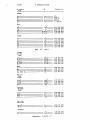
SI CONVERSION
FACTORS
Multiply By
To
Convert
From
Length:
2.54
0.025 4
0.304 8
0.914 4
609 344
ft
yd
ml
AEes
2
Hectares
Hectares
sere
6.451
9.290
8.361
2.589
4.046
600
304
274
988
856
2.957
4.731
9.463
3.785
1.638
2.831
7.645
353
765
529
412
E+O0
E-02
E-OI
E+02
E-O1
Volume
m
oz.
m
qt,
m
m
m
m
yd
m
NOTE:
Volume
per Unit
Time
ft•/s--in./mln,
yd =/mln,
gs I/min,
oz
Ib
ton
Im
3
1,000
(2000 ib)-
E-05
E-04
E-04
E-03
706 E-05
685 E-02
549 E-01
L
m•/sec
•3
ft
3
3
3
3
3
3
3
m3/sec----m3/sec----m3/sec---/sec"
•
4.719 474 E-04
2.831 685 E-02
2.731 177 E-07
1.274 258 E-02
6.309 020 E-05
ks,
kg
ks,
kg
2.834
1.555
4.535
9.071
952
174
924
847
E-02
E-O3
E-01
E+02
4.394
2.767
1.601
5.932
185
990
846
764
E+OI
E+04
E+OI
E-Of
3.048
4.470
5.144
1.609
000 E-01
400 E-Of
444 E-01
344 E+O0
6.894
4.788
757
026
E+03
E+O1
1.000
1.000
000
000
E-06
E-Of
Mesa per
Unit
Volume:
Ib/yd•
lb/±.•
lb/f•
g/m 3
kg/m
kg/m
lb/yd
3
Velocity:
(Includes
Speed)
ft/e.
mi/h.
knot
km/h
mt/h.
Force
Unit
Per
Area:
Ibf/ln•
lbf/ft
z
Viscosity:
m2/s
cS
pt
Ps ",•
Temperature
°F-32)5/9
°C
AN EVALUATION OF SIGNAL TIMING AND COORDINATION
Volume I:
Technical
PROCEDURES
Report
by
E. D. Arnold, Jr.
Research Scientist
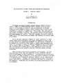
INTRODUCTION
The Manual on Uniform Traffic Control Devices (MUTCD) defines a
traffic signal as a power-operated traffic control device by which
traffic is alternately directed to stop and permitted to proceed.
Signals are most commonly used at street intersections to control the
assignment of vehicular or pedestrian right-of-way; thus, they exert a
significant influence on traffic flow. Signals that are warranted and
are properly designed, installed, and operated provide for the orderly,
efficient movement of traffic. They also increase the traffic handling
capability of the intersection and reduce the frequency of certain types
of accidents.
One of the most important elements of signal operation is signal
can be defined as the proper assignment of time to the
various vehicular or pedestrian movements at a particular intersection.
As compared to a correctly timed signal, a signal timed improperly can
result in increases in delay, in gasoline consumption and air pollution,
and in certain types of accidents.
Signal timing has received a great
deal of attention in recent years as the importance of utilizing the
existing transportation system in the most efficient manner has been
timing, which
recognized.
There are many signal timing procedures and strategies, and they
vary according to the type and capability of the controller and the
traffic requirements at the intersection.
Pretimed and vehicle-actuated
controllers are timed differently, as are the signals located at isolated
intersections, at intersections along an arterial, and at intersections
in a system network.
Further, the timing procedures range from simple,
manual techniques to comprehensive techniques applicable to mainframe or
minicomputers. Techniques are available or are being developed for the
microcomputer.
PURPOSE AND SCOPE
Accordingly, the main purpose of the study was to compile in a
single document recommended procedures for timing the various types of
signals. Specifically, procedures are included for both pretimed and
vehicle-actuated controllers located at isolated intersections and at
intersections in a signal system. Simplicity and ease of use are
emphasized in the procedures as the targeted users are field technicians
and those responsible for maintaining signals in small cities and towns.
The procedures are based on a synthesis of the pertinent literature.
Finally, brief descriptions of popular computer programs which calculate
timing are included.
A secondary purpose was to survey jurisdictions responsible for
signals in Virginia to determine the types of equipment being utilized.
The survey was conducted through a mail-back questionnaire to all cities
and towns, the two counties that maintain signals, and the Department of
Highways and Transportation's field offices.
FORMAT AND USE OF REPORT
A separate Field Manual sets forth the recommended procedures in a
simplified, steR-by-step manner exclusive of detailed, background
discussion.
Designed for the most part to stand by itself, the Field
Manual is intended to provide the user with concise and easily applied
procedures for timing the various types of signals. The Technical Report
provides the user with the theory and logic underlying the summarized
procedures in the Field Manual and should be reviewed to obtain a
thorough understanding of timing.
Also, some of the definitions and timing procedures are applicable
In these cases, the information is
to more than one category of signals.
often duplicated for the convenience of the user.
INVENTORY OF
EQUIPMENT
A survey was conducted to determine the types of control equipment
The questionnaire in Appendix A was
use in the state of Virginia.
65
and
the
2
cities
counties that maintain signals, and
sent to
towns,
the 9 construction districts of the Virginia Department of Highways and
Transportation. Responses were received from 26 cities, 16 towns, 2
counties, and 9 construction districts. Following is a summary of the
survey results.
in
Manufacturers
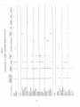
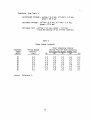
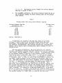
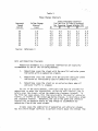
Table 1 shows the responding jurisdictions and the manufacturers of
the signal controllers that each has. The most commonly used controllers in Virginia were manufactured by Crouse Hinds, Automatic Signal, or
Eagle. It is interesting to note that the Department utilizes the
largest variety of manufacturers, partly because of the large number it
maintains and partly because it continually purchases equipment on a low
bid basis.
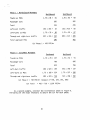
Isolated Intersections
Based on the responses received, essentially all of the Department's
signalized intersections are actuated
approximately 20% operate semiactuated, 50% operate fully actuated, and 30% operate fully actuated with
volume-density timing. On the other hand, local jurisdictions, especially small cities and towns, maintain a significant number of pretimed
signals. Seventeen percent of the isolated intersections are under
pretimed control, whereas 26% are semi-actuated, 48% are fully actuated,
and 9% are fully actuated with volume-density timing.
Signal Systems
The
Department maintains
46 systems,
all of which
are
arterial
Approximately 200 intersections are included in these systems,
and the majority of these operate semi-actuated.
Twenty-six of the
systems utilize time-based coordinators, whereas the other 20 are
hard-wired through a street master controller.
systems.
Local jurisdictions reported a total of 82 systems with 919
intersections.
Sixty-three are arterial systems. Fifty-nine percent of
the intersections in the systems operate pretimed, 25% operate
semi-actuated, 13% operate fully actuated, and 3% operate fully actuated
with volume-density timing. Only 13% are coordinated through time-based
coordination; the remaining 87% have hard wire interconnection. Eightytwo percent of the interconnected systems are controlled by a street
master, 14% by a central computer, and 2% by a time clock.
3
•,4
•
X
X
XX
4
XX
Auxiliary Equipment
Tn recent years the functions performed by auxiliary, stand-alone
equipment have been incorporated into the signal controller itself. The
Virginia Department of Highways and Transportation, as well as several
local jurisdictions, reported that the stand-alone equipment is being
phased out as quickly as possible. Of the stand-alone equipment
remaining, the most common types by far are minor movement controllers
and coordination
units.
Detectors
type of detector in use in Virginia is the inductive
Six of the Department's construction districts reported
actual numbers of detectors, and 80% are loop detectors and 20% are
magnetic detectors. For the districts providing estimated percentages of
each kind of detector, the average percentages are 65% loops, 30%
magnetics, 2% magnetometers, and 3% radar.
The most
detector.
loop
common
For those local jurisdictions which reported actual numbers of
was found that 77% of the detectors are loops, 13% are
magnetics, 8% are magnetometers, and 2% are pressure sensitive. For
those 7 •urisdictions reporting a percentage breakdown by tyDe of
detector, the average percentages are 80% loops and 50% magnetics.
detectors, it
Availability
o#
Computers
Computers are becoming increasinaly available at
the Department, four of the districts reported
microcomputer.
Within
a
the local level.
the availability of
At the local level, 6!% of the respondents indicated the
of a computer, with 30% of those havinQ access to a
mainframe, 7% to a mini, and 63% to a microcomputer. The various models
of IBM computer are the most common.
Of particular note is the tact that
10 of the 17 microcomputers are IBM.
availability
Conclusions
Based
on
the results of the questionnaire survey regarding types of
in the state, the following general conclusions can be
signals utilized
made.
Controllers manufactured
Technologies), Automatic
by Crouse-Hinds {now called Traffic Control
Signal, and Eagle are the most common in
Virginia. This is the
obtained in 1976.
finding reported
same
in
an
inventory
Department maintains only 4 pretimed signals at isolated
On the other hand,
are actuated.
approximately 17% of the signals at isolated intersections reported
by local jurisdictions are pretimed. Old, pretimed equipment is
quite common in the small cities and towns. Therefore, it is still
important to discuss timing procedures for pretimed signals.
The Department maintains 46 signal systems, whereas 44 of the 67
local jurisdictions maintain 82 systems. All of the Department's
systems are arterial systems, whereas 63 of the local systems are
arterial systems.
The remaining 19 are grid systems.
The
intersections; the remainder
Over 1,100 intersections are known to be in a system. The
majority of the local jurisdictional intersections operate pretimed,
whereas the majority of the Department's intersections in a system
operate semi-actuated. This is explained by the fact that the 19
grid systems reported by local jurisdictions contain predominantly
pretimed intersections.
Of the Department's 46 systems, 26 use the new time-based
coordination.
Only 11 of the local jurisdictional systems use
time-based coordination.
This is explained by the fact that the
Departmen• is continually upgrading and expanding its signal
systems. Due primarily to budget constraints, cities and towns
cannot do this on a routine basis.
Auxiliary, stand-alone equipment is generally being phased out
through modernization programs as the functions performed by this
equipment are built into the new replacement controllers.
Auxiliary equipment that is still commonly found includes minor
movement
controllers
and coordination units.
Inductive loop detectors are the most commonly used type.
For those
respondents reporting actual numbers of detectors, it was found that
there are approximately 5,700 loops, or 78% of the total number of
detectors.
The next most common, at 1,200 and 17%, are magnetic
detectors.
detectors.
Computers
There
are
only
a
few magnetometers,
radar, and pressure
level.
are available to a limited extent at the local
Seventeen of the responding jurisdictions have microcomputers,
whereas another 10 have access to a mini or mainframe computer.
Only 4 of the Department's construction districts reported the
availability of a microcomputer; however, the other 5 should be
receiving micros shortly. Thus, the use of signal timing computer
programs
Virginia.
is feasible
for many of the
agencies maintaining signals
in
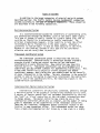
TIMING FOR PRETIMED SIGNALS AT ISOLATED INTERSECTIONS
Background
A pretimed controller operates according to a predetermined
schedule; that is, it has a fixed cycle length which is subdivided into
discrete, preset phases to accommodate required individual traffic
This type of equipment is best suited when traffic patterns
movements.
are predictable and do not vary significantly.
flexibility in timing as most controllers allow for at least
independent timing plans, which are generally based on time
and volumes
of week variations
in the traffic
patterns.
There is
three
of day or
some
day
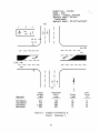
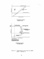
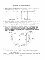
Definitions
See
1.
2.
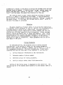
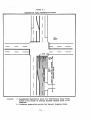
The following definitions are applicable to timing pretimed signals.
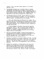
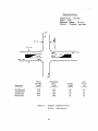
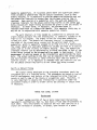
Figure 1.
Timing plan a unique combination of cycle length and split.
Cycle • the time required for one complete sequence of signal
indications.
that part of a signal cycle allocated to any combination of
traffic movements simultaneously receiving the right-ofway during one or more intervals.
3. Phase
one
or
4. Interval
5.
signal
Split
phases.
more
a discrete portion of the
indications remain unchanged.
the
percentage of
a
signal cycle during
cycle length allocated
which the
to each
of the
Cycle
Phase l
Main St.
Second
St.
G
R
Red
Interval
Figure
1.
Timing
Y
•
Interval
sequence for
R
G
Yel 1 o'w
Interval
simple two-phase controller.
Objective
The major objective of signal timing is to assign the right-of-way
traffic movements so that all vehicles are accommodated with
alternate
to
Short cycle
of delay to any single group of vehicles.
minimum
amount
a
lengths minimize average delay, or delay to single groups of vehicles,
provided the capacity of the cycle to pass vehicles is not exceeded. If
there is a constant demand, however, long cycles will accommodate more
vehicles over a given period of time because there is a lower frequency
of starting delays and clearance intervals between phases. Satisfying
the objective of signal timing, therefore, results in conflicting
requirements for the cycle length. Thus, the objective should be
restated to that of determining the shortest cycle length which will
accommodate the traffic demand, within certain limits.
Timing
Procedures
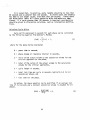
A summary of the recommended procedures for timing a pretimed signal
The basic concepts for each step along with appropriate
is listed below.
examples of using the procedures are described in the remainder of this
Because of the relationships among physical data, type of
section.
equipment, timing plans, and phasing, it may be necessary to undertake
steps i through 3 simultaneously if a new signal is being installed.
timing plans needed.
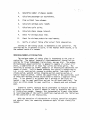
1.
Determine the number of
2.
Collect necessary information at the intersection.
Y
Determime
number of
phases needed.
equivalents.
4.
Calculate passenger
5.
Find critical
6.
Calculate optimum
7.
Calculate cycle splits.
8.
Calculate
9.
Check #or minimum
phase
I0.
Check for minimum
pedestrian requirements.
11.
Verify
or
car
lane volumes.
cycle length.
phase change interval.
time.
ad.iust timing after actual field observation.
of the timing values is dependent on the controller.
be in percent of cycle, to the nearest whole second,
the nearest tenth of a second.
Setting
settings may
Determine Number of
Timing
The
or
to
Plans
The maximum number of timing plans is determined by the tvpe of
controller.
The typical three-dial electromechanical cnntroller can
provide for three independent timing plans, one per dial. The modern
microprocessor-based controller is generally capable of a total of 12
plans, a combination of at least four cycles and three splits. The
variation or pattern of traffic demand at an intersection determines the
number of plans.
Traffic demand patterns are typically categorized as
a.m. or p.m. peak period, average or midday Deriod, late night or low
volume period, weekend period, shopping period, evening period, or
special function period. Within the capabilities of the controller, each
of these well-defined periods would normally receive a separate timing
plan. It can generally be assumed that a minimum of two plans are
needed
Two
one for peak conditions and one for off-peak conditions.
plans are often needed for peak condition
inbound peak and outbound
peak.
Extensive traffic counting may be undertaken to evaluate the daily
weekly variations in traffic demand in order to determine the number
of timing plans needed.
However, this determination is most often based
knowledge of the traffic conditions coupled with the limitations
on local
or
of the controller at the intersection.
and
With the exception of information on existing controller equipment
physical data, the remaining procedures appl.v to each timing plan
needed.
Collect
Necessary
Intersection
Information
Basic information concerning the intersection must be obtained in
order to apply the actual timing procedures described later. Following
is a description of the minimum data needed to calculate signal timing.
Effective timing is dependent upon the accuracy of the input data.
Control
Equipment
Knowledge of the control equipment already at the intersection
equipment to be installed is mandatory. The controller's timing
or
functions and their characteristics and limitations must be known.
In
the case of equipment already at the intersection, information on its
timing, especially the number of timing plans and phases, is important to
know.
Physical
The
geometrics
Data
following
information
at the intersection
Number of
or
should be obtained.
approaches
Number of lanes and
turn,
concerning the physical dimensions and
combination)
type of flow (through, right turn, left
per lane for each approach
Width of lanes and medians
grade
4.
Percent
5.
Speed limits
6.
Location of
zones, etc.
Traffic and Pedestrian
on
approaches,
if
severe
parking, crosswalks, stop bars,
bus stops,
loading
Data
In order to apply the timing procedures described later, hourly
traffic volumes and pedestrian counts are needed on every approach to the
intersection.
Further, the approach traffic should be categorized into
the number of vehicles turning left, going straight through, and turning
right. It. is also necessary to count and record the number of buses and
large trucks per hour on each approach. Finally, the average speed of
traffic approaching the intersection on each leg should be obtained.
I0
hourly information is needed for each timing plan determined
For example, a three-dial controller may have a timing plan for
the morning peak period, a lunch or midday period, and an afternoon peak
period. In order to calculate the timing for each plan, the above
described hourly information representative of these three periods must
Likewise, traffic and pedestrian data for weekends, nights,
be obtained.
and special functions must be obtained in order to calculate the timing
for these periods.
It is noted that data collected on Tuesdays,
Wednesdays, and Thursdays are more representative of average weekday
conditions than those collected on Mondays and Fridays.
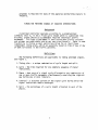
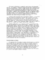
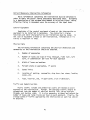
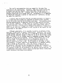
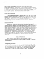
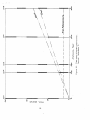
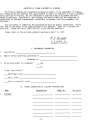
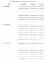
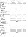
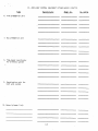
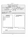
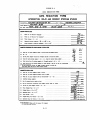
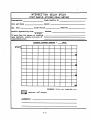
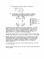
A typical data collection form is provided in Figure 2. It is noted
that the volumes are tabulated by one-half hour intervals during the
This
earlier.
normal mornino and afternoon rush hours. This enables a more accurate
determination of peak-hour statistics than would be possible with
one-hour summaries.
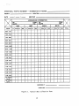
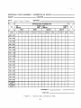
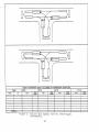
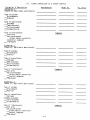
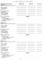
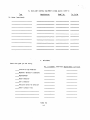
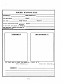
Volume counts by 15-minute intervals would be the
Figures 3 and 4 show other common forms used to summarize
most accurate.
the data for 3-1egged and 4-1egged intersections, respectively.
Although undesirable, it is possible to derive an estimate of the
peak-hour volume based on general relationships. Generally, the 12-hour
volume between 7:00 a.m. and 7:00 p.m. is from 70% to 75% of the 24-hour
volume and the peak-hour volume is from 10% to 12% of the 24-hour volume.
Thus, if either a !2- or 24-hour count is conducted or known, then the
peak-hour volume can be estimated. Further, approximately 60% of the
traffic volume during the peak hour is in the heavier direction in
suburban areas.
In central areas the approximatepercentage in the
heavier direction of flow is 55%. As an example of the usage of these
relationships, a 12-hour count at an intersection in a suburban setting
shows a volume of 700 vehicles.
Thus, the 24-hour volume can be
estimated at 1,000 vehicles and the peak-hour volume, which generall.y
Finally, the
occurs in the afternoon, can be estimated at 100 vehicles.
approach
volumes
be
estimated
vehicles
60
and
40
vehicles.
two
It
at
can
is emphasized that actual traffic counts provide much better timing than
counts estimated from these relationships.
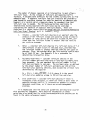
Determine Number of Phases
As a general rule, the number of phases should be kept to a minimum.
Cycle lenqths that are long result in delays to individual groups of
vehicles awaiting the green indication; therefore, there are practical
limits to cycle lengths in order to avoid these intolerable d•lays.
Accordingly, additional phases tend to decrease the available green time
for other phases since they must be accommodated within the practical
maximum cycle length.
Also, there is additional lost time throuqh
delays
and
phase
change or clearance intervals over the course
start-up
of a c.vcle as the number of phases increases.
11
DIRECTIONAL
INTERSECTION
MOVEMENT
TRAFFIC
OF
ROUTES
LOCATION
COUNTY
DATE
WEATHER
/.--..--
I
ON
ROUTE
EAST
HOURS
THRU
RT.
INTERSECTION
APPROACHING
FROM
THE
WEST
PED.
LT.
JTHRUI
RT.
FROM
THE
ON
ROUTE
SOUTH
NORTH
PED.
LT.
THRL•
RT.
PED.
LT.
6:00.7:00
7:00
7:30
7:30
8:00
8:00
8:30
S:30
g:00
9:00- 10:00
10:00- 11:00
11:00
12:00
12:00. 1:00
1:00
2:00
2:00
3:00
3:00
4
4:00
4:30
4:305:00
5:30
5;30
6:00
12 HOUR
"I'•TAL
24 HOUR
TOTAL
RECORDED BY
SUPERVISOR
Figure 2.
Typical
data collection
12
form.
THRLJ
RT.
PED.
TOTAL
EIGHT MAXIMUM
TIME
RTE.
TO
FROM
HOUR
VOLUMES
OF APPROACH
RTE.
VEH.
RTE.
VEH.
CROSS.
VEHICLES
FED.
CROSS.
TOTAL
VEH.
PEO.
CROSS.
TOTAL
Figure
3.
Typical
data
intersection.
summary
13
form for
three-legged
VEH.
PED.
CROSS.
EIGHT
TIME
FROM
VOLUMES
PED.
VEH.
CROSS.
OF
APPROACH
VEHo
PED.
CROSS.
VEHICLES
TOTAL
RTE.
RTE.
RTE.
RTE.
TO
HOUR
MAXIMUM
VEH.
PED.
CROSS.
VEH.
PED,
CROSS.
TOTAL
Figure
4.
Typical
data
summary
intersection.
14
form for
four-legged
VEH.
PED.
CROSS.
The number of phases required at an intersection is most often a
left-turn issue. As the volumes of left-turn and opposing traffic
increase, it becomes more difficult for the traffic turning left to find
adequate gaps. A separate left-turn lane can alleviate the problem to
some degree by providing storage for vehicles awaiting an adequate gap;
however, at a certain point a separate phase for movement from that
left-turn lane is needed.
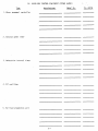
The following guidelines applicable to
intersections having separate left-turn lanes may be used when
considering the addition of separate left-turn phases. These are
contained in a recent report entitled Guidelines for Exclusive/Permissive
Left-Turn
Signal Phasina, by
Volumes
consider
B. H.
Cottrell, Jr.(•)
phasing
left-turn
on
an
approach
when
the
product of the left-turn volume and opposing volume divided bv
the number of lanes during the peak hour exceeds 50,@00, provided that the !eft-turn volume-is qreater than two vehicles
per cycle on average.
Delay
consider left-turn phasing if a left-turn delay of ?.0
vehicle-hours or more occurs in the peak hour, provided that
the left-turn volume is greater than two vehicles per cycle on
Also, the average dela.v per left-turning vehicle must
average.
be at least 35 sec.
See Appendix B for a procedure for
determining intersection delay.
Accident experience
consider left-turn phasing if the
critical number and resulting rate of left-turn accidents have
been exceeded.
For one approach the critical number is five
left-turn accidents in one year. The accident rate, as defined
by the annual number of left-turn accidents per I00 million
left-turn plus opposing vehicles, must exceed the critical rate
determined by the equation
Rc
32.6
left-turn
+
1.645-•32.6/M
0.5 M, where M is the annual
in I00 million vehicles.
plus opposing volume
consider left-turn phasing if there is
inadequate sight distance, if there are three or more lanes
opposing through traffic, if intersection geometrics promote
hazardous conditions, or if there are access management
problems.
Site conditions
It is emphasized that
engineering #udgement.
guidelines plus guidelines
with
found
the above are guidelines and should be
More detailed information on these
for using protected/permissive phasing
in the above referenced report.
15
of
coupled
can
be
Calculate
Passenger
Car
Equivalents
The timing procedures described later require that volumes be known
The use of PCEs
in terms of passenger car equivalents (PCE) per hour.
accounts for the negative impacts of trucks, buses, and turning vehicles
Trucks and buses
on the traffic handling capability of an intersection.
also require more
but
they
automobile,
than
only
not
an
occupy more space
Trucks having 6
characteristics.
acceleration
their
time
due
to
start-up
equivalent of
the
considered
should
be
intercity
buses
and
tires
or more
of the
the
vicinity
stopping
in
Local
buses
1.75 passenger cars.
intersection have even greater negative impacts than do intercit• buses,
and should be estimated to be the equivalent of 5.0 passenger cars.
Turning vehicles also have an adverse impact on intersection
operation. Left-turning vehicles which must yield to oncomi•q vehicles
should be considered the equivalent of 1.•5 passenger cars, and rightturning vehicles .yielding to pedestrians on the cross street should be
estimated at 1.25 passenger cars •f the number of right turns is more
It is noted that
than 1•% or the number of pedestrians is significant.
the
above factors
however,
used;
equivalency
sometimes
factors are
other
later. See
described
procedures
with
the
timing
are recommended for use
Table 2 for a summary of the PCE factors.
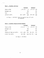
Table 2
Passenger
Type
Trucks
of Vehicle
(6
or
more
Intercity Buses
Local
or
Car
Equivalents (PCE)
PCF Factor
Movement
tires)
!e.g., Trailways/Greyhound)
1.75
1.75
5.O0
Buses
Left-turns with
Factors
Opposing
1.75
Traffic
Right-turns Conflicting with Pedestrians (more
than 10% right turns)
16
1.25
As an example, consider the case of an intersection having
significant pedestrian flow and a total approach volume on one leg of
1,000 vehicles, of which 10% are intercity buses and trucks, 2% are local
transit buses, 15% are left turns, and 12% are right turns. The
following steps illustrate the calculation of PCEs for the approach.
Adjust for vehicle types
Number of
intercity
Number of local
buses and trucks
PCEs
buses
PCEs
Number of passenger
Adjust for turning
100
880
PCEs
1.0
880
PCEs
175+100+880
1,155
1,155
174
305
or
left-turning vehicles
right-turning
PCEs
vehicles
PCEs
Number of
through vehicles
880
x
15%
1.75
12%
1.25
x
x
x
x
174
1,155
•
139
174
842
842
1,155-174-139=
PCE•
Total Approach PCEs
Find Critical
27
movements
Number of
Number
100
175
1,000-100-20
cars
Total
10% x 1,000
1.75 x 100
2% x 1,000
5.0 x 20
1.0
x
842
305+174+842
1,321
Lane Volumes
A critical lane volume (CLV) is the highest lane volume in vehicles
(vph) for a particular phase. In this step the CLV for all
hour
per
phases must be determined and then summed over the entire intersection.
If enough green time is provided to handle the lane having the highest
volume during a phase, then there automatically is sufficient green to
accommodate other lanes of traffic moving during that phase.
The
following general rules apply to calculating the CLV.
I.
CLVs
are
calculated in PCEs.
Right-turn and left-turn movements are considered part of
through movement unless there are exclusive turn lanes.
17
the
Exclusive left-turn and right-turn lanes without separate
phasing should be assigned the appropriate number of PCEs as
determined by the 1.75 factor for opposing traffic to
left-turns or the 1.25 factor when right turns are more than
10% or pedestrian flow is significant. The turning volumes
should then be compared directly with the through volumes to
determine the CLV.
If the left-turn movement is protected from conflict with
separate phasing, the adjustment factor of 1.75 is not applied.
When 2 approach lanes handle through traffic, it should be
assumed that the critical lane carries 55% of the volume.
Likewise, for 3 approach lanes the critical lane is assumed to
carry 37% of the volume.
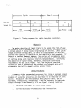
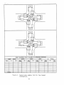
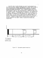
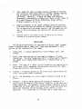
As
Following
an
example,
are
consider the intersection shown in Figure 5.
the steps necessary to obtain the CLV for each phase.
18
Characteristics
Pedestrians
Buses
none
minimal
Approach speeds
25 mi/h
Control
2-phase, pretimed
375
28
ft..__•
N
44 ft.
747
864
•
290
Approach
Northbound
Southbound
Eastbound
Westbound
Total
Vo ume
Passenger
Cars
Trucks
Left
Turns
290
375
864
747
255
322
786
695
35
53
78
52
10
12
20
25
Figure 5.
(vph)
(vph)
Example intersection A.
Source:
19
Reference
2.
(%)
North/South Movement
1
Phase
Southbound
Northbound
Trucks
1.75
PCEs
as
x
35
61
1.75
53
x
93
Passenger Cars
255
322
Total
316
415
10%
Left-turn traffic
Left-turns
Through
Total
1.75
PCEs
as
x
right-turn
approach PCEs
and
x
90%
traffic
x
316
32
12%
32
56
1.75
316
284
88%
PCEs
Passenger
Cars
1.75
x
78
Total
Through
as
and
PCEs
right-turn
CLV Phase 2
As
a
x
415
365
Westbound
738 PCE/hr
1.75
52
91
786
695
923
786
185
25%
x
786
197
1.75
x
185
324
1.75
x
197
345
80%
x
923
738
75%
x
786
590
+
738
of 738, 324, 345,
590)
1,190 PCE/hr
second example, consider the intersection shown in
are the steps necessary to obtain the CLV for each
20
x
923
(largest
452
137
x
traffic
CLV Total
Following
87
20%
Left-turn traffic
Left-turns
50
x
452 PCE/hr
1
East/West Movement
as
50
452
Eastbound
Trucks
415
340
CLV Phase
Phase 2
x
Figure 6.
phase.
Pedestrians
Buses
none
minimal
3-phase, pretimed
Approach speed 45 mi/h
north/south.
Approach speed 55 mi/h east/west
Control
710
1
2
3
1,036
Approach
Northbound
Southbound
Eastbound
Westbound
Total
Volume
Passenger
Cars
Trucks
831
710
748
625
995
891
83
85
(vph)
(vph)
1,036
948
Figure 6.
Example
Source:
21
intersection B.
Reference 2.
(vph)
41
57
Left
Turn
(%)
12
14
19
24
s
East/West Left-Turns
Phase 1
Eastbound
Trucks
as
PCEs
Passenger
cars
1.75
x
Left-turn traffic
CLV Phase
I
19%
(factor
238 PCE/hr
are
East/West
Phase 2
Through
and
applied
not
unopposed)
Right
as
PCEs
Passenger
cars
1,067
991
203
since
24%
x
41
Total
Citical
81%
lane traffic
x
55%
CLV Phase 2
22
991
x
238
left turns
Movements
1.75
Through and right-turn traffic
100
891
Eastbound
Trucks
57
x
995
1,067
x
1.75
72
41
Total
Westbound
x
Westbound
72
x
57
100
995
891
1,067
991
1,067
864
864
475
475 PCE/hr
1.75
76%
55%
x
x
991
753
753
414
North/South Movement
Phase 3
Trucks
as
PCEs
Passenger
cars
1.75
x
83
Total
Left-turn traffic
Left-turns
Through
Total
as
and
1.75
x
85
149
748
625
893
774
12%
x
893
107
14%
x
774
108
1.75
x
107
187
1.75
x
108
189
88%
x
893
786
86%
x
774
666
right-turn traffic
approach
Critical
PCEs
145
PCEs
973
lane traffic
55%
x
973
535
855
55%
x
855
470
CLV Phase 3
535 PCE/hr
CLV Total
238 + 475 + 535
1,248
Calculate
Optimum C•¢le Length
As stated earlier, the specific objective of timing a pretimed
is to determine the cycle which minimizes average delay and will
also accommodate the traffic demand. One such technique, Webster's
Method, accomplishes this through the equation
signal
1.5L
1-Y
23
+
5
(1)
where
C
cycle length
in seconds which minimizes
delay
at the
intersection,
L
total
lost time per
seconds/phase,
cycle
in seconds,
typically
4.0 to 5.0
and
total of the ratios of the actual volume to the saturation
volume for the critical approaches, with saturation volume
typically
in the range
1,700
to
1,800 vph.
The delay at the intersection is reasonably constant in the range of
0.75 C to 1.50 C; therefore, a good estimate of C can still be obtained
If
even when simplifying assumptions are made for the above equation.
the lost time per phase is assumed to be 4.0 seconds and the saturation
volume is assumed to be 1,800 vph, then equation 1 is modiified as
follows.
6N+5
1
CLVT
(2)
1,800
where
before,
C
as
N
number of
CLV T
phases,
and
sum of CLVs per phase in PCEs/hr for
the intersection.
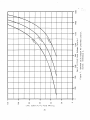
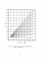
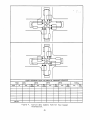
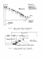
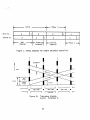
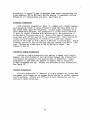
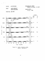
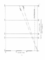
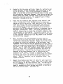
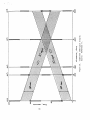
graphical solution to equation 2 is presented in Figure 7, and in
cases the optimum cycle can be determined directly from the graph.
As an example of the use of Figure 7, consider the previous example
intersections A and B. Intersection A has 2-phase control and a CLV T of
1,190,
1,190 PCEs/hr. If Figure 7 is entered on the horizontal axis at
vertical
axis
from
the
read
be
cycle
of
50
seconds
optimum
across
can
an
from the 2-phase curve. Similarly, the 1,248 PCEs/hr at the 3-phase
intersection in example B has an optimum cycle of 75 seconds.
A
most
24
(•es) t4•Bual aLDZD *•L•C]
25
ttlntucU.LIN
It is noted that, in practice, cycle lengths should be no less than
In recent years the tendency
40 seconds and no greater than 120 seconds.
has been to use longer cycles, even more than 120 seconds. Timing above
and below these limits will cause excessive delay and motorists impaIf a cycle greater than 120 seconds is required, consideration
tience.
should be given to alternative solutions, such as intersection modifications.
Calculate
C•cle Splits
Cycle splits expressed in seconds for each phase
by the following equation from Webster's Method.
(G+A)
Y
-(C-L)
+
can
be calculated
(3)
I,
Y
where for the
phase being considered
G
green time in seconds,
A
phase change
y
ratio of the actual volume to.the saturation volume for the
critical approach for the phase.,
Y
total
or
clearance
interval
of the ratios of the actual
volume for the critical
approaches,
in
volume to the saturation
C
cycle length
L
total lost time per cycle in seconds,
seconds per phase, and
l
lost time for the
in
seconds,
seconds,
typically 4.0
to 5.0
phase.
As before, the above equation can be modiified if an average lost
time of 4.0 seconds and a constant saturation volume is assumed for all
phases.
(G+A)
CLV(C-4N)
CLV T
26
+
4,
(4)
where
(G+A)
phase
time in seconds
CLV T
C
of CLVs per
sum
cycle length
in
phase
PCEs/hr,
in
in PCEs/hr for the intersection,
seconds, and
phases.
number of
N
defined before,
phase being considered
CLV for
CLV
as
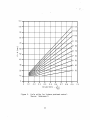
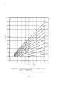
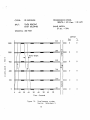
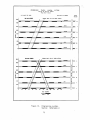
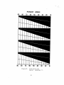
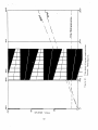
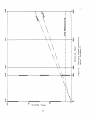
Graphical solutions to equation 4 are presented in Figures 8 through
10 for 2-, 3-, and 4-phase control, respectively.
In most cases splits
The total of the phase times
can be obtained directly from the graphs.
should equal the known cycle length. Again, the previously described
intersections A and B can be used to exemplify the use of the graphs.
2-phase,
Intersection A:
50 sec, CLV
1
738 PCE/hr, CLV T
CLV 2
CLV1/CLV T
452/1,190
452 PCE/hr,
C
0.38 and
1,190 PCE/hr
CLV2/CLV T
738/1,190
0.62
Therefore, from Figure 8,
Entering 0.38
Entering 0.62
to the 50 sec
to the 50
sec
line, (G+A) 1
line, (G+A) 2
Total
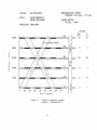
3-phase,
Intersection B:
CLV 2
CLV T
CLV1/CLV T
CLV3/CLV T
20 sec,
30 sec, and
50
sec.
75 sec, CLV
238 PCE/hr,
1
475 PCE/hr, CLV 3
535 PCE/hr,
C
1,248 PCE/hr
238/1,248
0.19,
535/1,248
0.43
CLV2/CLV T
475/1,248
0.38, and
Therefore, from Figure 9,
to the 75
sec
line, (G+A)
1
16 sec,
0.38 to the 75
sec
line, (G+A)
2
28 sec,
0.43 to the 75
sec
Entering 0.19
Entering
Entering
27
line, (G+A) 3 31
Total
and
sec,
75
sec.
II0
C=120
I00
C:110
9O
C=lO 0
8O
C
90
C
80
7O
•
+
C= 70
C= 60
50
4O
3O
2O
I0
0.I
0.2
0.3
0.5
0.4
Volume
Figure
8.
Ratio
Cycle splits
Source:
for 2-phase
Reference 2.
28
0.7
0.6
0.8
V
VTOT
pretimed control.
0.9
1.0
II0
I00
C=120
//•//C=IO0
C=IlO
9O
8O
7O
•
60
C= 70
+
/
50
C
60
4O
3O
2O
I0
0
Figure
0.I"
9.
0.2
0.3
0.4
Volume
for 3-phase
Reference 2,
Cycle splits
Source:
0.5
Ratio
29
0.6
0.7
0.8
V
VTOT
p•etimed
control.
0.9
1.0
II0
100
C=120
9O
8O
C=IO0
70
•
+
60
C
50
70
40
30
lO
0.I
0.2
0.3
0.4
0.5
0.6
Volu.le Ratio
Figure
lO.
Cycle splits
Source:
for
Reference
30
0.7
0.8
0.9
V
VTOT
4-phase pretimed
2.
control.
1.0
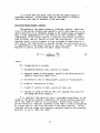
It is noted that the phase times include the phase change
clearance interval. Actual green time for each phase is found
subtracting that time as obtained in the next step.
Calculate Phase
Chan•e
or
by
Interval
The purpose of the phase change or clearance interval, which consists of the yellow interval and, possibly, an all-red interval, is to
advise motorists of an impending change in the right-of-way assignment,
that is; the commencement of a red interval on their approach.
Upon
commencement of the change interval, a motorist should have sufficient
time to either stop his vehicle or clear the intersection.
At a given
approach speed, a certain amount of time is needed to decelerate to a
safe stop at the intersection or proceed through the intersection prior
to commencement of the green interval on the cross street.
The following
equation is used to calculate the phase change interval.
CP
t
+
v
2a+64,4g+
w+__LL
(5)
V
where
a
change period in seconds,
perception/reaction time, usually 1.0 second,
approach speed in feet/second, typically the 85th percentile
speed or prevailing speed limit,
deceleration rate in feet/second 2, usually 10 feet/second 2,
W
width of intersection
L
length
CP
t
V
g
of vehicle
in
in
feet,
feet, usually 20 feet, and
percent of grade divided by 100, with upgrade being positive
and
downgrade being negative.
It is important that motorists have a reasonable expectation of the
of the yellow interval; therefore, the yellow interval should be
the range of from 3.0 to 5.0 seconds.
Within these limits, the
interval is often set according to the time it takes to decelerate
to a stop; that is, the first two terms in the above equation.
Yellow
intervals that are longer than necessary decrease capacity and encourage
motorists to try to "beat the light."
length
set in
yellow
31
The time needed to clear the intersection as calculated by the last
term in the above equation should be included in an all-red interval
Required stopping time
where all approaches receive a red indication.
above 5.0 seconds should also be included in the all-red interval.
phases do not typically have an all-red interval.
phase follows the exclusive turn movement;
through-movement
a
therefore, motorists receiving the green directly face straggling
left-turners and can safely yield the right-of-way. An all-red interval
may be needed, however, at a high-speed intersection or at an
Exclusive turn
Normally,
intersection with
a
wide median.
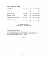
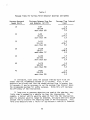
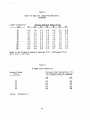
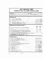
Equation 5, minus the grade factor, coupled with the aforementioned
rules regarding the phase change interval have been used to develop the
information in Table 3. For a given approach speed, the yellow change
interval plus the total phase change interval for various intersection
The all-red interval is the difference between the
widths are presented.
intervals.
It
is sometimes the practice to round up the
given
two
intervals to the nearest 0.5 second.
As an example of the use of Table 3,
described intersections A and B.
Intersection A:
again consider
approach speed,
25 mi/h
north/south
street
east/west street
all
previously
the
approaches
ft, (G+A) 1 20 sec
30 sec
44 ft, (G+A) 2
28
Therefore, from Table 3,
north/south
st.
yellow
green
yellow
east/west st.
green
Intersection B:
3.0 sec, all-red
15.4 sec
1.6 sec,
3.0 sec, all-red
25.8 sec
1.2 sec,
approach speed, north/south
mi/h approach speed, east/west
56 ft, (G+A)
north/south through
76 ft, (G+A) 2
east/west through
45 mi/h
55
east/west left
32
(G+A)
1
16
sec
31
3
28
sec
sec
Therefore, from Table 3,
north/south through
yellow
4.3 sec, all-red
25.2 sec
green
east/west through
yellow
5.0 sec, all-red
22.0 sec
green
east/west left
yellow
{note
5.0 sec, green
11.0
the absence of an all-red
1.5 sec,
1.0 sec,
sec
interval)
Table 3
Phase
Change
Intervals
Total Clearance Interval
(Yellow Plus
for Crossing
Approach
Speed
(mi/h)
Yel low Change
Interval
( sec
30
50
20
25
30
35
40
45
5O
55
3.0
3.0
3.2
3.6
3.9
4.3
4.7
5.0
4.2
4.2
4.3
4.5
4.8
5.1
5.3
5.7
4.9
4.7
4.8
4.9
5.1
5.4
5.6
5.9
Source:
Reference 3.
33
All-Red Clearance)
Street Widths (ft)
70
90
5.5
5.3
5.2
5.3
5.5
5.7
5.9
6.2
6.2
5.8
5.7
5.7
5.8
6.0
6.2
6.4
II0
6.9
6.4
6.2
6.1
6.1
6.3
6.4
6.7
Check for Minimum Phase Time
For safety reasons, due primarily to motorists' expectations, there
minimum values on the timing of the phases at an intersection operating under pretimed control. These minimums, including the clearance
interval, are 15 seconds for through movements and 12 seconds for turning
A quick review of the timing derived for the example intermovements.
sections will show no violation of these minimums.
are
Should these minimums be violated, the phase timing should be
increased to the minimum and the time added to the total cycle length.
Check •or Minimum Pedestrian
Requirements
Pedestrian movements at a signalized intersection
accommodated by one of the following methods:
Pedestrians cross the street with the
indication with no pedestrian signals.
Pedestrians
indication
parallel
are
typically
vehicular green
with the parallel vehicular
by special pedestrian signals.
cross the street
as instructed
Pedestrians cross the street
vehicular traffic is stopped.
on
an
exclusive
green
phase when all
For any of the above methods, sufficient time must be provided for
to enter the intersection, called the walk interval, and to
safely cross the street, called the pedestrian clearance interval. In
the first two cases above, the time needed for pedestrians occurs while
the parallel vehicular traffic, or traffic on the street not beina
crossed, is receiving a green and clearance interval. Therefore, the sum
of the green and clearance interval for an approach should be long enough
to accommodate any pedestrian flow on the cross street.
pedestrians
In man.v cases the combination of pedestrian and vehicular volumes
may not create enough conflicts to warrant a check for the minimum time
At locations where there are significant
needed by pedestrians.
pedestrian volumes or pedestrians require special attention, such as near
elderly housing, it is necessary, however, to calculate the needed
crossing time and compare it with the time allocated to the movement of
parallel vehicular traffic. The walk interval, or time needed by a
pedestrian to perceive the signal change and move into the intersection,
The higher values
is generally assumed to be from 4.0 to 7.0 seconds.
clearance
pedestrian
high.
The
pedestrian
volumes
when
used
are
are
interval is dependent upon the width nf the street being crossed and the
walking speed of the pedestrian, which is generally assumed to be 3.5 to
The slower speeds are used when pedestrian volumes are
4.0 feet/second.
high or in special cases such as in the vicinity of elderly housing.
34
Except for the special 'situations mentioned, the following general
equation is applicable. Field measurement of walking speeds at the
intersection would provide the best data.
(G+A•min.
5
(6•
W/4,
+
where
IG+A)
minimum green
approach
width
W
median.
interval
in seconds
on
being crossed.
in feet of the street
of very wide streets with a median, it may be judged
allow
only enough time for pedestrians to safely reach the
to
The entire crossing would then require the timing of two cycles.
In the
acceptable
not
plus phase change
being crossed, and
case
I s the phase in question does not meet the minimum pedestrian
requirements, the timing should be increased to the minimum and the cycle
length adjusted accordingly.
The previous
of eauation 6.
example intersections
north/south
Intersection A:
north/south
(G+A)
28 ft,
street
east/west street
Check:
be used to illustrate
can
44
28/4
5
+
+
44/4
(G+A)?
ft,
12
sec
20
1
30
the
use
sec
sec
less than 30
so
o.k.
east/west
5
east/west through
north/south
Check:
east/west
or
#t, (G+A) 3
76 ft,
(G+A)•
(G+A)
east/west !eft
5
16
1
56/4
5
+
+
76/4
less than 20
sec
56
north/south throuqh
Intersection
Verify
16
19
24
31
28
o.k.
so
sec
sec
sec
sec
sec
less than 58
less than 31
sec
sec
so
so
Adjust Timing
The signal
considered only
timing developed by
a starting point.
as
the preceding procedures should he
The procedures are based on typical
35
Ook.
o.k.
performance, and factors at the intersection being timed may
modify some of the theory or assumptions used. Therefore, it
is very important to observe the intersection in operation under the
calculated timing in order to either verify the settings or adjust them
traffic
negate
or
if necessary.
TIMING
FOR ACTUATED SIGNALS AT ISOLATED
INTERSECTIONS
Background
A traffic-actuated controller operates in response to traffic
demand.
Detectors on the roadway "advise" the controller of the Dresence
of vehicles, and that oarticular movement or phase receives a green
That phase retains the green as long as sufficient demand
indication.
exists, or until a preset maximum time has been reached. Then the
controller switches the areen to another phase which has been called due
Thus, within the constraints of the
to the detection of a vehicle.
preset maximum times, the controller provides continuously variable cycle
lengths and phases in accordance with actual demand. This type of
control is very efficient as it allocates the right-of-way based on real
time demand, not on the basis of an assumed demand distribution as is the
It is interesting to note that when the
case with pretimed control.
traffic flow is heavy for all movements, the actuated controller
functions in pretimed operation with the cycle length and phase times
being governed by the preset maximumtimes.
Definitions
The
signals.
following qeneral definitions
Cycle
the time
indications.
required
for
are
one
apolicable
complete
to
timing actuated
sequence
of
signal
Phase
that part of a siQnal cycle allocated to any
combination of one or more traffic movements simultaneol•sly
receiving the right-of-way during one or more intervals.
Detector
a device which detects the passage or presence of a
vehicle with the purpose of advising a controller of the need
For purposes of this project,
for a green indication.
detectors will be categorized as either small area detectors or
large area detectors. Small area detectors provide passage,
point, motion, or unit detection. These detectors simply
register the passage of a vehicle. It is noted that a 6 x
Large area
6-foot loop is often used as a point detector.
These detectors
detectors provide presence or area detection.
36
register the presence of a vehicle in the zone of detection.
As will be discussed later, the timing can vary with the type
and location of the detectors.
Gap
distance between successive vehicles crossing a point
the roadway.
For signal timing the "distance" is usually
measured in seconds.
Types
Equipment
of
The three distinct types of actuated
subsections.
following
Semi-actuated
on
equipment
are
described
in the
Controllers
The best use of a semi-actuated controller at an isolated
intersection is where the major street volumes are high compared to the
minor street volumes.
The major street phase is not actuated; therefore,
the right-of-way always returns to the major street when there are no
vehicles present on the minor street or when the minor street's maximum
This type of operation is also used where
green time has been reached.
the controller is incorporated into a signal system. The nan-actuated
phase is coordinated with ad.iacent intersections while the actuated
phases are allowed to respond to detected demand within certain
limitations.
Followingis a list of characteristics of semi-actuated
control.
Detectors are located
the intersection.
on
only
the minor street
The major phase, or non-actuated
minimum green interval.
The major phase green extends
a call from the minor street.
phase, receives
approaches
a
to
preset
indefinitely until interrupted
The minor phase receives a green
if the major phase has completed
bv
indication after it is called
its minimum green interval.
The minor phase receives a preset minimum green; however, the
green will be extended by additional calls until a preset
maximum green time is reached or until a preset gap in traffic
occurs.
If the green time is terminated by the Dreset maximum, a memory
feature automatically returns the right-of-way to the minor
street once the ma,!or street receives its minimum green.
37
The yellow change and all-red clearance
for each phase.
intervals
are
preset
Full-actuated Controllers
Full-actuated control has traffic actuations for all phases. This
is used at isolated intersections where traffic volumes
significantly
throughout the day and where there is not a large
vary
The
difference between volumes on the major and minor streets.
operational characteristics were generally defined in the previous
Following are specific characteristics of
section on background.
full-actuated operation.
type of control
I.
Detectors
are
located
on
all
approaches
to the
intersection.
Each phase receives a preset minimum green; however, the green
w•ll be extended by additional calls until a preset maximum
green time is reached or until a preset gap in traffic occurs.
The yellow change and all-red clearance
for each phase.
intervals
are
preset
Volume-density Controllers
Volume-density
control is also fully actuated; however, added
enable
features
a more comprehensive evaluation o •, and thus response to,
The
traffic conditions than does the basic full-actuated operation.
actual
the
accommodate
be
extended
minimum
to
oreset
so as
green can
Likewise, the preset gap.
number of vehicles awaiting the right-of-way.
reduced
time,
be
measured
in
which is
so as to be more sensitive to
can
offers particular
volume-density
features
flow.
The
of
traffic
use
detectors
approaches
where
high-speed
advantages on
are located several
characteristics
Specific
the
intersection.
hundred feet from
are as
follows:
1.
Detectors
are
located
on
all
approaches
to the
intersection.
Each phase receives a minimum green which can be extended
additional vehicles queue up at the red indication.
Once the minimum or extended minimum green is
green is maintained by additional calls until
is reached or a preset gap in traffic occurs.
volume-density control, the preset gap can be
period of time so that the green is terminated
occurrence of a smaller gap than necessary at
38
as
reached, the
a preset maximum
In the case of
reduced after a
at thp
first.
The yellow change and all-red clearance
for each phase.
Phase Control
Each phase on
control functions
intervals
are
preset
Functions
actuated controller has several switches which
modes of operation for that phase. Although these
specifically
related to timing, it is important to be
functions are not
Following is a brief description of the modes.
aware of their operation.
an
or
Lock Detector
When a vehicle actuates a detector on a phase which is set in the
lock detector m•de, that call is "locked in" the memory of the controller
until such time as that phas• is serviced, or receives a green
Small area or point detectors require that the controller be
indication.
set in this mode.
Non-lock Detector
A phase set in the non-lock detector mode sends a call to the
controller only if a vehicle is present in the detection zone. Once the
vehicle moves out of the zone, the call for-service is cancelled.
Large
This mode of operation
area or presence detectors require this setting.
is appropriate for locations where right-turn-on-red occurs and for
left-turn phases with exclusive-permissive control.
Non-actuated
A phase set in the non-actuated mode automatically operates under
semi-actuated control, with that phase controlling the ma.ior street or
non-actuated traffic flow.
Recall
When the recall switch on a phase is on, the controller
If all recall
returns to that phase during each cycle.
switches are activated, the controller automatically cycles through all
phases. Tn this case the controller operates in a pretimed manner and
all advantages of actuated control are lost.
•f no recall switches are
activated, the controller stays in the last serviced phase indefinitely
until a call is received from another phase.
automatically
There are several variations
is set when the detectors
recall"
of this mode.
are
39
functioning,
If "minimum vehicle
the controller
automatically returns to the phase to service the minimum green and then
operates based on demand. A "vehicle recall to max" setting causes the
phase's maximum green interval to time out. Finally, a "pedestrian
recall" setting causes the pedestrian intervals to time out.
The "vehicle recall to max" switch should be activated to ensure
It may be beneficial
service to a phase if the detectors are broken.
during periods of low volume to have the controller "resting" in green
•n this case the "minimum vehicle recall" switch on
the major street.
the main line phase is activated.
on
Objective
The ma•or objective of signal timinQ is to assign the right-of-way
traffic movements so that all vehicles are accommodated with
alternate
to
Actuated control is
•f delay to any single group.
minimum
amount
a
responsive within certain limitations to traffic demand, and thus can
provide very efficient operation at an intersection. Unlike pretimed
control, cycles and phases vary in timing and sequence. Thus, timing
actuated controllers involves the understanding of and setting of the
preset intervals, or timing parameters, alluded to in the previous
These parameters must be set for
discussion on types of controllers.
each phase in the cycle.
Timing
Procedures
As indicated earlier, the essential part of timing actuated
intersections is the setting of values for the timing parameters.
Several other steps are necessary, however, and following is a list of
The basic concepts and, if applicable,
the recommende• procedures.
described
in the remainder of this section.
suggested settings are
information
at the
intersection.
1.
Collect necessary
2.
Determine number of
3.
Determine
values
4.
Verify
ad.•ust timing after field observation.
or
for
phases needed.
timing parameters.
Setting of the timing values is dependent
settings may be to the nearest whole second or
second.
40
the controller.
The
tenth
of
the
nearest
to
on
a
Collect
•ecessary Intersection Information
Basic information concerning the intersection must be obtained in
order to apply the actual timing procedures described later.
Following
is a description of the minimum data needed to calculate signal timing.
Effective timing is dependent upon the accuracy of the input data.
Control
Equipment
Knowledge of the control equipment already at the intersection
equipment to be installed is mandatory. The controller's timing
or
functions and their characteristics and limitations must be known.
In
the case of equipment already at the intersection, information on its
timing is important to know.
Physical Data
The
following
geometrics
information
at the intersection
Number of
concerning
the physical
should be obtained.
dimensions
approaches
Number of lanes and type of flow (through, right turn,
turn, or combination} per lane for each approach
Width
left
of lanes and medians
grade
4.
Percent
5.
Speed limits
6.
Location of
zones,
and
on
approaches,
if
severe
parking, crosswalks, stop bars, bus stoDs, loading
etc.
Type, location, and,
if
applicable,
size of detectors.
Traffic and Pedestrian Data
Hourly traffic volumes and pedestrian counts are needed on every1
approach to the intersection. Further, the approach traffic should be
categorized into the number of vehicles turning left, going straight
through, and.turning right. It is also necessary to count and record the
number of buses and large trucks per hour on each approach.
Finally, the
speed
of
traffic
approaching
intersection
the
each
leg should
average
on
he obtained.
41
The traffic and pedestrian data are needed for the peak-flow
Typically, peak flow occurs during the
condition at the intersection.
afternoon rush period; however, side street peak flow may occur at
another time during the day. Likewise, peak flow at the entrance to a
shopping center may occur around 9:00 p.m. Accordingly, it is important
to obtain the data over a period of time which will definitely include
the peak-flow condition.
data collection form was provided previously in Figure 2.
It is noted that the volumes are tabulated by one-half hour intervals
during the normal morning and afternoon rush hours. This enables a more
accurate determination of peak-hour statistics than would be possible
Volume counts by 15-minute intervals would be
with one-hour summaries.
Figures 3 and 4 showed other common forms used to
the most accurate.
summarize the data for 3-1egged and 4-1egged intersectiops, respectively.
These figures have been reproduced in this section of the report for the
convenience of the reader.
A
•ipical
Although undesirable, it is possible to derive an estimate
peak-hour volume based on general relationships. Generally, the
of the
12-hour
volume between 7:00 a.m. and 7:00 p.m. is from 70% to 75% of the 24-hour
volume and the peak-hour volume is from 10% to 12% of the 24-hour volume.
Thus, if either a 12- or 24-hour count is conducted or known, then the
peak-hour volume can be estimated. Further, approximately 6•% of the
traffic volume during the peak hour is in the heavier direction in
In central areas the approximate percentage }n the
suburban areas.
heavier direction of flow is 55%. As an example of the usage of these
relationships, a 12-hour count at an intersection in a suburban settipg
Thus, the 24-hour volume can be
shows a volume of 700 vehicles.
estimated at 1,000 vehicles and the peak-hour volume, which generally
Finally, the
occurs in the afternoon, can be estimated at 100 vehicles.
It
two approach volumes can be estimated at 60 vehicles and 40 vehicles.
is emphasized that actual traffic counts provide much better timing than
counts estimated from these relationships.
42
DIRECTIONAL
MOVEMENT
TRAFFIC
INTERSECTION
ROUTES
LOCATION
COUNTY
_.._._1•
DATE
OF
/•
WEATHER
APPROACHING
ON
ROUTE
EAST
HOURS
6:00
7:00
7:00
7:30
LT.
THRU
RT.
INTERSECTION
FROM
ON
THE
ROUTE
WEST
PED.
LT,
THRU
RT.
FROM
THE
SOUTH
NOR TH
PED.:
LT.
THRLJ
RT.
PED.
7:30. 8:00
8:00
8:30
8:30
g:O0
9:00. 10:0•
10:00
11
11:00
12:0•
12:00
1:00
1:00
2:00
2:00
3:00
3:00
4:00
4:00
4:30
4:30- 5:00
5:00
5:30
5;30
12 HOURTOTAL
24 HOUR
TOTAL
RECORDED BY
SUPERVISOR
Figure
2.
Typical
data
43
collection
form.
LT.
THRU
RT.
PED.
TOTAL
I_mJ
EIGHT MAXIMUM
FROM
VEH.
TO
VOLUMES
OF APPROACH
PEO.
CRO,•.•.
VEHICLES
TOTA L
RTE.
RTE.
RTE.
TIME
HOUR
VEH.
VEH.
CRO•.
PED.
CROSS.
TOTAL
Figure
3.
Typical
data summary
intersection.
44
form
for
three-legged
VEH.
PED.
CROSS.
EIGHT
TIME
FROM
VEH.
VOLUMES
PED.
CROSS.
VEH.
OF
APPROACH
PED.
CROSS.
VEH.
VEHICLES
RTE.
RTE.
RTE.
RTE.
TO
HOUR
MAXIMUM
PED.
CROSS.
VEH.
TOTAL
PED.
CROSS.
TOTAL
Figure 4..,Typical
data summary form for
intersection.
45
four-legged
VEH.
PED.
CROSS.
Determine Number of Phases
As a general rule, the number of phases should be kept to a minimum.
Cycle lengths that are long result in delays to individual groups of
vehicles awaiting the green indication; therefore, there are practical
limits to cycle lengths in order to avoid these intolerable delays.
Accordingly, additional phases tend to decrease the available green time
for other phases since they must be accommodated within the practical
maximum cycle length. Also, there is additional lost time through
start-up delays and phase change or clearance intervals over the course
of a cycle as the number of phases increases.
The number of phases required at an intersection is most often a
left-turn issue. As the volumes of left-turn and opposing traffic
increase, it becomes more difficult for the traffic turninq left to find
adequate gaps. A separate left-turn lane can alleviate the problem to
some degree by providing storage for vehicles awaiting an adequate pap;
however, at a certain point a separate phase for movement from that
The following guidelines applicable to
left-turn lane is needed.
intersections having separate left-turn lanes may be used when
considering the addition of separate left-turn phases. These are
contained in a recent report entitled Guidelines for Exclusive/Permissive
Left-Turn Signal Phasing, by B. H. Cottrell, Jr.(•)
consider left-turn phasing on an approach when the
of the left-turn volume and opposing volume divided by
the number of lanes during the peak hour exceeds 50,000,
provided that the left-turn volume is greater than two vehicles
per cycle on average.
Volumes
product
consider left-turn phasing if a left-turn delay of 2.0
vehicle-hours or more occurs in the peak hour, provided that
the left-turn volume is greater than two vehicles per cycle on
Also, the average delay per left-turning vehicle must
average.
See Appendix B for a procedure for
be at least 35 sec.
determining intersection delay.
Delay
cnnsider left-turn phasing if the
Accident experience
critical number and resulting rate of left-turn accidents have
For one approach the critical number is five
been exceeded.
The accident rate, as defined
left-turn accidents in one year.
by the annual number of left-turn accidents per 100 million
left-turn plus opposing vehicles, must exceed the critical rate
determined by the equation
Rc
32.6
left-turn
+
1.645-•32.6/M
0.5 M, where M is the annual
in 100 million vehicles.
plus opposing volume
46
consider left-turn phasing if there is
inadequate sight distance, if there are three or more lanes
opposing through traffic, if intersection geometrics promote
hazardous conditions, or if there are access management
problems.
Site conditions
of
It is emphasized that the above are guidelines and should be coupled
engineering, judgement. More detailed information on these
guidelines plus guidelines for using protected/permissive phasing can be
with
found in the above referenced report.
Determine
Values
for the TiminQ
Parameters
In recent years, traffic control equipment has become reasonab!.v
standardized by the National Electrical Manufacturers Association (NEMA).
Thus, the models of equipment manufactured in recent years have basicall.v
the same dials and settings, and employ the same terminology.
Accordingly, the following discussion on timing parameters will focus on
the NEMA controllers; however, information on pre-NEMA equipment will
also be presented where possible.
It is very important to be familiar
with the timing functions of the equipment being retimed or being
considered in the case of a new installation.
The phase timing for a NEMA traffic-actuated controller is shown
Figure 11, and a typical phase timing for older equipment is shown in
Figure 12. Both of these figures are referenced in the following
discussion of timing parameters.
in
The following general rules concerning the timina of
traffic-actuated controllers are often cited. These are contained in the
International Municipal Signal Association's Traffic Signal Manual.(•)
Make all timing ad.iustments during
controller will then automatically
traffic efficiently.
heavy traffic.
take
care
of the
The
light
Set the dials at values considered correct after evaluating
detector spacing, relative volumes, and desired results.
Then,
adjust or "tune" the controller to accommodate the heaviest
traffic.
After the dials have been set, take steps
unauthorized persons cannot change them.
The tendenc.v is to set the times
settings produce snappier,
operation.
Timing parameters
must
more
be established
47
too
high.
efficient
to
ensure
In
that
general, lower
intersection
for each phase.
"X"
Detector Actuation
Phase wdh
Right-of.Way
The Initial Stale
ngN-of-way
tl•e
time. It will De
Minimum Green t•me, tl•e
Passage
time. the AdO•
Indial t•me
(in V•u•e Density aoplicat•ons)
Unexpired Portions of
t•e sum of the Walk an• P•estnan
Passage Time Pe•od.
CleM•¢e time, wh•ev•
longest.
timing.
Start of Gree•
Figure ii.
Typical timing diagram
NEMA controller.
for a full-actuated
Reference 5.
Source:
Maximum
Initial
Figure 12.
Reset
Vehicle
Minimum Green Time
Interval
i I
/
TimingM°del 80"NDiagram
Typical timing diagram
non-NEMA controller.
48
for a full-actuated
Reference 2.
Source:
Passage
Time
For the typical, low-speed intersection, the passage time, which has
also been referred to as the vehicle interval or unit extension interval,
is defined as the time needed for a vehicle moving at average speed to
travel from the detector to and through the intersection. As shown in
both Figures 11 and 12, this interval begins to retime itself when a
vehicle actuates the detector.
Retiming continues upon each actuation
until such time as the maximum time setting is reached; then, the
controller switches to another phase that has been called. This operation is referred to as "force off" or "max out." If a vehicle does not
receive a full passage time interval because of being forced off or an
actuation is received during the yellow change interval, the controller
Thus, the green is
assumes the vehicle did not clear the intersection.
automatically returned to that phase at the earliest opportunity. On the
other hand, if a gap in traffic is large enough such that the passage
time is reached before being re-actuated, then the phase ends and the
controller switches to another phase that has been called. This is often
called a "gap out." Accordingly, the passage time has two functions
it allows vehicles to travel from the detector through the intersection,
and it establishes the gap, measured in seconds, at which green is
terminated.
At intersections where speeds are 35 mi/h or less, and where small
area or point detectors are used, the needed passage time is calculated
by dividing the distance between the intersection and the detector by the
However, the gap required to retain
average approach speed of traffic.
the green must also be cbnsidered.
Bumper-to-bumper traffic produces
of
from
2.0
3.0
seconds,
with
the former being indicative of
to
gaps
fast-paced, urban areas and the latter being more likely in rural areas.
Passage times set in this range make the operation too sensitive to gaps.
On the other hand, gaps greater than about 5.0 seconds cater to the
"stragglers" in the traffic stream and cause a reduction in efficiency.
Detectors are typically located such that the passage time falls in this
Therefore, the passage time interval at intersections where
range.
speeds are 35 mi/h or less and point detectors are used should be set to
the nearest tenth of a second as calculated by dividing the detector
spacing by the average approach speed; however, it should be no less than
3.0 seconds and no more than 5.0 seconds.
Table 4 summarizes these
rules.
49
Table 4
Passage Times for Various Point
Average Approach
Speed (mi/h)
15
20
Distance Between
and Detector (d)
30
35
40
45
Stop
(ft)
Bar
Spacings
and
0-111
112-181
more than
3.0
d/22.0
5.0
3.0
0-89
90-i45
than
Speeds
Passage Time Interval
(sec)
0-67
68-108
more than 108
more
25
Detector
d/29.3
145
5.0
3.0
d/36.7
!81
5.0
0-134
135-217
more than 2].7
d/44.0
0-156
157-253
more than 253
d/51.3
0-179
180-290
more than 290
d/58.7
0-201
202-326
more than 326
d/66.0
In slow-paced, rural areas the passage time may have
higher than the recommended minimum of 3.0 seconds. Also,
3.0
5.0
3.0
5.0
3.0
5.0
3.0
5.0
to be set
if the
detectors are placed such that the needed passage time is •reater than
5.0 seconds, it may be necessary to set the passage time interval abow
Doing this will decrease
the recommended maximum for safety purposes.
the efficiency of the intersection.
If large area or presence detectors are used at the stop bar, very
For
little time is needed for a vehicle to clear the intersection.
example, a typical vehicle would be about 20 feet into the intersection
•vhen its presence would no longer be detected, and would need only enough
Also,
passage time to traverse the remaining width of the intersection.
large area detectors have a "built-in" gap because a vehicle is detected
50
for a finite period of time as it traverses the detector.
This gap can
be calculated by adding the length of the loop and an assumed 20 feet for
the length of the vehicle and dividing by the average speed of vehicles
The built-in gaps for various lengths of detectors and
on the approach.
approach speeds are given in Table 5. Accordingly, when large area
detectors are used at intersections having speeds of 35 mi/h or less, the
following procedures should be undertaken to determine the passage time
interval.
Select the gap required to retain the green, which, as
discussed above, should be between 3.0 and 5.0 sec. As a
general guideline, a gap of from 3.0 to 4.0 sec is good for
•ast-paced, urban areas or where snappy operation is desired,
and a gap of from 4.0 to 5.0 sec is qo•d for slow-paced, rural
areas.
From Table 5 determine the built-in gap for the size of the
detector used and the average speed.
Calculate the setting for the passage time interval by
subtracting the built-in gap from the gap required to retain
the green selected in step 1. This setting is usually between
1.5 and 3.0 sec in most applications.
In the case of very long
detectors and slow speeds, the detector's built-in gap may be
the same or even exceed the gap selected to retain the green;
therefore, the setting on the passage time dial conceivably
could be zero.
high-speed intersections, defined generally as
having speeds greater than 35 mi/h, is treated somewhat differently. Since most high-speed intersections are controlled by the Virginia Department of Highways and Transportation, the two most common
types of operations are described in this report. The first treatment
considers the fact that at high speeds the decision to stop or continue
at the onset of a yellow clearance interval becomes a much more critical
issue than at slow speeds.
The area in which this indecision occurs is
called the dilemma zone. Motorists caught outside the dilemma zone, or
away from the intersection, generally reach the decision to strip when a
yellow indication is observed. Motorists inside the dilemma zone, or
toward the intersection, generally decide to proceed through the
intersection.
The boundaries of the dilemma zone are given in Table 6.
The passage time at
those
.51
Table 5
Built-ln Gaps for Large Area Detectors
(Seconds)
Average Approach Speed (mi/h)
Length of Detector
(ft)
15
20
25
30
35
40
45
20
30
40
50
60
70
80
90
100
110
120
1.8
2.3
2.7
3.2
3.6
4.1
4.5
5.0
5.5
5.9
6.4
1.4
1.7
2.0
2.4
2.7
3.1
3.4
3.8
4.1
4.4
4.8
1.1
1.4
1.6
1.9
2.2
2.5
2.7
3.0
3.3
3.5
3.8
0.9
1.1
1.4
1.6
1.8
2.0
2.3
2.5
2.7
3.0
3.2
0.8
1.0
1.2
1.4
1.6
1.8
1.9
2.1
2.3
2.5
2.7
0.7
0.9
1.0
1.2
1.4
1.5
1.7
1.9
2.0
2.2
2.4
0.6
0.8
0.9
Based on the formula [length of detector
1.47 ft/s.
and I mi/h
(ft)
+
1.1
1.2
1.4
1.5
1.7
1.8
2.0
2.1
20]/speed (ft/s)
Table 6
Dilemma Zone Boundaries
from Intersection (ft)
for Probabilities of Stopping
Approach Speed
Distance
(mi/h)
35
40
45
50
55
Source:
Reference 6.
52
10%
90%
102
122
152
172
234
254
284
327
353
386
Two small area or point detectors are used on each approach lane.
The first is placed a distance corresponding to a travel time of from 2.0
to 4.0 seconds at the average speed outside an imaginary line located
within the dilema zone at which 90% of the motorists will decide to
proceed through the intersection. This is the 10% probability of stopping distance in Table 6. The second detector is placed the same 2.0 to
4.0 seconds of travel time beyond the first detector. This configuration
is shown in Figure 13. The passage time is then set at the same 2.0 to
4.0 seconds, and actuation of either detector will cause the interval to
retime itself. A single vehicle traveling at the average speed will be
ensured consecutive 2.0- to 4.0-second intervals which will place the
vehicle at the aforementioned 90% line when a yellow clearance signal is
received.
Likewise, a single vehicle traveling above or below the
average speed will find itself inside or outside the dilemma zone,
respectively.
Detector
2.0
(2.0
4.0
4.0
2.0
sec
x
1
ft/s)
d
(2.0
Detector
4.0
4.0
sec
x
10% Probability
of Stopping
Distance
for
Approach Speed
Figure
13.
High-speed approach detection.
53
ft/s)
2
advantage of dual detection is that there are more chances of
the green for that phase. Since the phases having dual
detection receive favored treatment, this type of design is most often
used when the main line volumes and speeds are high as compared to those
An
extending
of the side street.
In summary, if this
the passage time should
design must be reviewed
of obtaining the setting
by the average approach
slow down after crossing
design is encountered in a retiming situation,
The original
be set at 2.0 to 4.0 seconds.
Another method
setting.
determine
the
to
proper
is to divide the distance between the detectors
speed. If there is a tendency for vehicles to
the second detector, for example in the case of
the passage time may be set up to 1.0 second
that there is less chance of motorists being
right-turning vehicles,
design time so
caught in the dilemma zone.
above the
If traffic volumesat a high-speed intersection are approximately
the same on all approaches, a volume-density operation is often employed.
The NEMA controllers have four or
This operation was described earlier.
volume-density
operation, three of which
for
five timing parameters
before reduction, the time
the
These
time
time.
involve the passage
are
the passage time of from
operation,
In
and
the
minimum
to reduce,
gap.
previously
for low-speed
described
determined
seconds,
3.0 to 5.0
as
needed
controls
the
to retain the
with
detectors,
point
intersections
gap
latter period
this
reduction"
Once
"time
period.
before
green during the
"time to
the
during
incrementally
decreases
the
times out,
passage time
reduce" period until the "minimum gap" is reached. This gap then
controls the phase until gap out or force off is attained. The lower
portion of Figure 14 shows gap reduction in a schematic form. Note that
gap reduction is initiated when a call is received on a conflicting
phase.
Since the gap reduction feature is intended to increase the
controller's response to traffic demand, it is necessary that these
settings be established based on field observations during the period of
Initial settings which should be adjusted on-site are
heaviest demand.
generally made based on logical considerations rather than a specific
methodology. The main purpose of gap reduction is to make the controller
increasingly sensitive to the traffic flow on the phase being serviced in
recognition of the waiting time a motorist on a conflicting phase is
experiencing.
54
VEHICLE ACTU&TIONS
EXPLANATORY DIAGRAM
VARIABLE INITIAL
Turn41
l'e,-- 11
RlgJllrlliOn
Co•ll•¢t•|
Of Slrvlclll•le
RIAI. TIM41 (Stcondl)
EXPLANATORY DIAGRAM
GAP REDUCTION
Figure 14.
Volume-density timing
Source:
Reference 2.
55
functions
(NEMA).
The controller is most sensitive to traffic flow when operating with
the minimum gap, and should maintain green only during bumper-to-bumper
traffic. Thus, a minimum gap setting of from 2.0 to 3.0 seconds will
usually be effective. If the phase being considered is relatively minor,
then the time to reduce can be rather short, e.g., 15 to 20 seconds. On
the other hand, the time to reduce on a major phase may be set at 30
seconds or more. The time before reduction is useful in delaying gap
reduction until slow-moving traffic such as large trucks can get in
motion. Another general rule of thumb is that the minimum gap should be
reached by the time the phase is at 80% of its maximum green time. The
split between time before reduction and time to reduce can be determined
according to the general logic just discussed.
Minimum Green
Actuated Phase
The minimum green interval for an actuated phase is set to allow
vehicles stopped between the detector and the intersection to get started
If small area or point detectors are
and move into the intersection.
being used, there is a finite distance between the detector and the
intersection in which vehicles can be stored while awaiting a green
indication. When the green is received, a minimum amount of green time
is needed to ensure that these stored vehicles can start up and move into
the intersection in case there are no further actuations to initiate
timing of the passage time interval. Studies have indicated that for a
single.line of vehicles, the time in seconds needed to accomplish this
can be estimated by the formula 2.1 n + 3.7, where n is the number of
vehicles. Assuming the average length of a vehicle is 20 feet, then the
number of vehicles can be estimated as the distance between the
intersection and the detector divided by 20 feet.
The minimum green timing parameter is shown schematically in
It is important to note from Figure 12 that for
11 and 12.
pre-NEMA controllers, the minimum green is the sum of a setting called
In this case,
initial interval plus the vehicle (passage time) interval.
the minimum green is calculated as described above, and the initial
interval is set by subtracting the vehicle interval.
Figures
In summary, the
is utilized
detection
procedure
is
as
for
determining
minimum green when
point
follows.
Determine the maximum number of vehicles, n, that can be stored
in a single lane between the stop bar and the point detector by
dividing the distance in feet between the two by 20 and
rounding up.
2.
Determine
the minimum green
56
setting by applying the formula
Application of this formula
n + 3.7.
spacings is given in Table 7.
2.1
for various
detector
For pre-NEMA controllers, the initial interval should be set as
the difference between the above minimum green and the passage
time interval.
Tabl
Minimum Green Time
versus
Distance Between Stop Bar
and Detector !ft)
7
Point Detector
Spacing
Minimum Green
(sec
0-40
41-60
61-80
81-100
!•I-120
121-140
Source:
e
7.9
10.0
12.1
14.2
16.3
18.4
Reference 3.
If detectors are located at the stop bar, there is no finite
distance in which a vehicle can be stored w•thout being detected.
Accordingly, the minimum green conceivably could be set at zero. There
considerations, most related to motorists' expectations,
are practical
however, which require that a minimum green time of between 4.0 and 7.0
seconds be set.
For high-speed intersections, the point detectors are typically
located a considerable distance from the intersection to allow a passage
time interval setting between 3.0 and 5.0 seconds.
A minimum green based
the
assumed
of
vehicles
that
results in excess
in
distance
storage
on
nreen being given to that phase when traffic is !iqht and the storage
In this case, a volume-density controller
space is not fully utilized.
is frequently used.
In order to utilize the volume-density function, an
additional timing parameter called "seconds per actuation" needs to be
Some NEMA controllers also have a parameter called "maximum added
•et.
initial". In operation, a minimum green time based on one vehicle is
set, that is, 2.1 seconds plus 3.7 seconds, or 5.8 seconds. Each
additional vehicle approaching the intersection during the nongreen time
will actuate the detector and increase the minimum green by the preset
seconds per actuation until such time as the maximum added initial green
time is reached.
This operation is depicted schematically in the upper
portion of Figure 14. In theory, the seconds per actuation should be set
at 2.1 seconds and the maximum added initial should be set to accommodate
the maximum storage in a single lane, as given by the previously
57
described formula, 2.1
This procedure is satisfactory for
in the case of a multi-lane approach,
should be set at 1.0 second.
n
+
3.7.
single-lane approach; however,
seconds per actuation
a
the
Again, volume-density settings should be based on field
Further, pre-NEMA controllers may have slightly different
for additional vehicles approaching the intersection;
account
to
ways
therefore, it is most important to review the instructions for the
specific controller being retimed.
observations.
Non-actuated Phase
Minimum Green
The minimum green interval for a non-actuated phase is applicable to
the major street at an intersection under semi-actuated control on which
there are no detectors to call or advise the controller of the presence
The major street is guaranteed a minimum green even if
of vehicles.
calls for service are incoming from the side street or from pedestrians.
If the side street demand is occasional and occurs randomly throughout
the day, then a relatively short setting of from 25 to 40 seconds should
On the other
be used to prevent excessive delay on the side street.
hand, in a situation where the side street discharges large numbers of
vehicles at certain times during the day, e.g. from a factory, with
almost no demand at other times, a relatively long setting of from 40 to
This ensures that the major street is not
60 seconds is appropriate.
interrupted too frequently during the period of heavy side street demand.
Minimum green should be calculated based on the relative traffic
volumes at the intersection. To accomplish this, it is assumed that
pretimed control exists, and minimum green on the major street, or for
the non-actuated phase, is compared with the maximum green for the side
street, or for the actuated phase. Then, the procedures for timing
pretimed controllers presented elsewhere in this report should be used.
The green time calculated for the non-actuated phase should be set on the
dials for both minimum green and maximum green on that phase. Other
settings are determined based on the actuated signal procedures.
Maximum Green
The maximum green interval
continuously moving traffic
been received
traffic flow
on
are
can
longest time that
signal once a call
operation, when gaps in
determines the
hold the green
a conflicting phase.
sufficiently small to
In
has
the
cause the passage time interval to
retime itself, the green is forced off because the maximum
value is reached rather than because the gap required to retain the green
If the passage time has been set correctly, the force-off
is exceeded.
condition is attained only during times of heaviest traffic flow at the
continuously
58
As mentioned previously, the controller is operating
intersection.
essentially in a pretimed fashion during heavy flow conditions because
all phases are being forced off at the preset maximum times.
Accordingly, the maximum green per phase for actuated control should be
determined in the same manner as the green time per phase is determined
for pretimed control. The reader is referred to the section of the
report on pretimed control.
Figures 11 and 12 depict schematically how the maximum green is
timed. As shown in Figure 11, the maximum green for NEMA controllers
begins timing upon receipt of a call on a conflicting phase. As shown in
Figure 12, the maximum interval for older controllers begins after the
initial interval has timed out. While it is not critical to take these
differences into account when setting the maximum green, it is important
to be aware of how the controller is timing when field checks are being
made.
Finally,
providing two
it should be noted that some controllers are capable of
maximum green intervals per phase. A time clock or other
external control selects the interval to be used. The timing would be
determined from two sets of volumes and pedestrian counts. An example
would be the use of a longer maximum green during peak hours than during
the remainder of the day.
Change
Yellow
and Red Clearance
The purpose of the phase change or clearance interval, which
consists of the yellow interval and, possibly, an all-red interval, is to
advise motorists of an impending change in the assignment of
right-of-way; that is, the commencement of a red interval on their
approach. Upon commencement of the change interval, a motorist should
have sufficient time to either stop his vehicle or clear the
intersection. At a given approach speed, a certain amount of time is
needed to decelerate to a safe stop at the intersection or proceed
through the intersection prior to commencement of the green interval on
the cross street. The previously presented equation 5 is used to
calculate the phase change interval.
CP
t
V
+
2a±64.4g
+
W+L,
V
where
CP
t
change period in seconds,
perception/reaction time, usually
59
1 second,
(5)
a
approach speed in feet/second, typically the 85th percentile
speed or prevailing speed limit,
deceleration rate in feet/second 2, usually 10 feet/second 2,
W
width of intersection
L
length
V
g
It is
of vehicle
in feet,
usually
in feet,
20 feet, and
percent of grade divided by 100, with upgrade being positive
downgrade being negative.
important that motorists have a reasonable expectation of the
and
length of the yellow interval; therefore, the yellow interval should be
Within these limits, the
set in the range of from 3.0 to 5.0 seconds.
yellow interval is often set according to the time it takes to decelerate
Yellow
to a stop; that is, the first two terms in the above equation.
intervals that are longer than necessary decrease capacity and encourage
motorists to try to "beat the light."
The time needed to clear the intersection as calculated by the last
term in the above equation should be included in an all-red interval
Required stopping time
where all approaches receive a red indication.
above 5.0 seconds
should also be included in the all-red interval.
Exclusive left-turn phases do not typically have an all-red
interval. Normally, a through-movement phase follows the exclusive turn
movement; therefore, motorists receiving the green directly face
straggling left-turners and can safely yield the right-of-way. An
all-red interval may be needed, however, at a high-speed intersection or
at an intersection with a wide median.
Equation 5, minus the grade factor, coupled with the aforementioned
rules regarding the phase change interval were used to develop the
information in Table 3. This table has been reproduced in this section
For a given approach speed, the
for the convenience of the reader.
yellow change interval plus the total phase change interval for various
The all-red interval is the
intersection widths are presented.
difference between the two given intervals.
60
Table 3
Phase
Approach
Speed
Total Clearance Interval
Plus All-Red Clearance)
for Crossin 9 Street Widths (ft)
(Yellow
Yellow Change
Interval
(mi/h)
(sec)
30
50
70
90
110
3.0
3.0
3.2
3.6
3.9
4.3
4.7
5.0
4.2
4.2
4.3
4.5
4.8
5.1
5.3
5.7
4.9
4.7
4.8
4.9
5.1
5.4
5.6
5.9
5.5
5.3
5.2
5.3
5.5
5.7
5.9
6.2
6.2
5.8
5.7
5.7
5.8
6.•
6.2
6.4
6.9
6.4
6.2
6.1.
6.!
6.3
6.4
6.7
20
25
30
35
40
45
50
55
Source:
Change Intervals
Reference 3
Walk and Pedestrian
Clearance
Pedestrian movements at a signalized intersection
accommodated by one Of the following methods:
Pedestrians cross the street with the
indication with no pedestrian signals.
Pedestrians
indication
cross the street
as instructed
are
typically
parallel vehicular
with the parallel
vehicular
by special pedestrian signals.
Pedestrians cross the street
vehicular traffic is stopped.
on
an
exclusive
green
Qreen
phase when all
For any of the above methods, sufficient time must be provided for
to enter the intersection, called the walk interval, and to
the street, called the pedestrian clearance irterval.
In
the first two cases above, this time occurs while the parallel vehicular
traffic, or traffic on the street not being crossed, is receiving a green
and clearance interval.
Therefore, the sum of the green and clearance
interval for an approach should be long enough to accommodate any
pedestrian flow on the cross street.
pedestrians
safely cross
In many cases the combination of pedestrian and vehicular volumes
may not create enough conflicts to warrant concern about the minimum time
61
needed by pedestrians.. At locations where there are significant pedestrian volumes or pedestrians require special attention, such as near
elderly housing, it is necessary to provide pedestrian actuation and set
the pedestrian intervals to ensure that the minimum crossing time is
received.
Upon receipt of a pedestrian call, the walk and pedestrian
clearance intervals for the phase controlling traffic on the street not
being crossed will begin timing and extend the green to the set values if
In other werds, if necessary, the minimum green is
necessar,v.
reestablished based on a pedestrian demand. This separate timing may or
may not be in conjunction with separate pedestrian siqnals.
The walk interval, or time needed by a pedestrian to perceive the
and move into the intersection, is generally assumed to be
The higher values are used when pedestrian
from 4.0 to 7.0 seconds.
volumes are high. The pedestrian clearance interval is dependent upon
the width of the street being crossed and the walking speed of the
pedestrian, which is generally assumed to be from 3.5 to 4.0 feet/second.
The slower speeds are used when pedestrian volumes are high or in special
Thus, the pedestrian
cases such as in the vicinity of elderly housing.
clearance interval can be determined by dividing the width in feet of the
Field
street being crossed by the assumed walking speed in feet/second.
measurement of walking speeds at the intersection would provide the best
data. The actual setting on the dial can be reduced by the yellow change
and red clearance intervals as these intervals must time out before a
It is important to remember that the intervals are set
conflict occurs.
traffic on the street no___•t being crossed.
controlling
the
phase
for
signal change
Verify
or
Adjust Timing
The signal timing developed by the preceding procedures should be
considered only as a starting point. The procedures are based on typical
traffic performance, and factors at the intersection being timed may
negate or modify some of the theory or assumptions used. Therefore, it
is very important to observe the intersection in operation under the
calculated timing in order to either verify the settings or adjust them
if necessary.
TIMING
FOR SIGNAL SYSTEMS
Background
A
signal system
consists of two
or
more
signalized
intersections
operated in coordination; that is, that have a f•xed time relationship
This relationship is based on the fact that vehicles at a
each other.
signal
are
released
in
platoons,
or
groups,
62
upon
receipt
of
a
green
to
indication and then travel in these platoons to the next signal. Thus,
it becomes desirable to establish a fixed time relationship between the
beginning of the green interval at the first intersection and the
beginning of the green interval at the second intersection such that the
platoon receives the green interval just as it arrives at the second
intersection.
This permits the continuous or progressive flow of traffic
along the street. When the coordinated intersections are located along a
single route, the term "arterial system" is applied. When two or more
routes cross at a common intersection, the result is a "signal network".
An open network has only one common intersection, whereas a closed
This latter network is
network has two or more common intersections.
often referred to as a "grid system," and is commonly found in the
Determination of the fixed time relationship
centers of large cities.
becomes increasingly difficult as the number of intersections in an
arterial system and the number of common intersections in a network
increase.
The effectiveness of coordinated control depends on whether traffic
be
kept in platoons between intersections. The ability to maintain
can
platoons depends on traffic characteristics, topography, condition of the
roadway, and roadside friction. As the distance between intersections
increases, the effects of these factors become more pronounced, and the
probability of platoon dispersal increases. The Manual on Uniform
Traffic Control Devices states that, "Traffic control signals within
0.5 mile of one another along a major route or in a network of
"
interconnecting major routes should be operated in coordination
Although this suggests a maximum spacing between signalized intersections
of 0.5 mile for effective coordination, there are many examples of
effective coordination where signals are spaced up to a mile apart,
particularly where roadside friction is minimal, speeds are high, and
signals are visible for some distance in advance of the intersection.
Generally, it is best to attempt to coordinate intersections if at all
possible to maintain traffic flow in platoons.
The following advantages of providing coordination among signals
listed in the Transportation and Traffic Engineering Handbook.(7)
higher level of traffic service
higher overall speed and reduced
A
is provided in terms
number of stops.
Traffic should flow more smoothly, often with
capacity and decrease in energy consumption.
an
are
of
improvement
in
Vehicle speeds should be more uniform because there will be no
incentive to travel at excessively high speed to reach a
signalized intersection before the start of the green interval,
yet slower drivers will be encouraged to speed up to avoid
having to stop for a red light.
63
There should be fewer accidents because platoons of vehicles
will arrive at each signal when it is green, thereby reducing
the possibility of red-signal violations or rear-end
collisions.
Naturally, if there are fewer red intervals
displayed to the majority of motorists, there is less likely to
be trouble because of driver inattention, brake failure,
slippery pavement, and so on.
Greater obedience to the signal commands should be obtained
from both motnrists and pedestrians because the motorist will
try to keep within the green interval, and the pedestrian will
stay at the curb because the vehicles will be more closely
spaced.
Through traffic
instead of
or
will
parallel
tend to stay on the arterial
minor streets.
street
Definitions
The
Figure
1
following definitions are applicable to timing signal systems.
depicted some of these, and it has been reproduced in this
section for the convenience of the reader.
1.
Timing plan
a
unique combination
of
cycle length, split,
and
offsets.
the time required for one complete sequence of signal
indications.
The term "background cycle" is often used to identify
the common cycle length established for all intersections in a
Cycle
system.
Phase
one
or
that part of a signal
more traffic movements
of-way during
4.
Interval
sigral
5.
Split
phases.
one
or
more
cycle allocated
of
of
intervals.
a discrete portion of the
indications remain urchanqed,
the percentage
to any combination
simultaneousl.v receiving the right-
a
signal cycle during
cycle length allocated
which
to each
the
of the
the passage or presence of a
•etector
a device which detects
vehicle with the purpose of advising a controller of the need for a
For purDoses of this project, Hetector• will be
green indication.
categorized as either small area detectors or large area detectors.
Small area detectors provide passage, point, motion, or unit
detection.
It is noted that a 6 x 6-foot loop is often used as a
64
point detector. These detectors simply register the passage of a
vehicle. Large area detectors provide presence or area detection.
These detectors register the presence of a vehicle in the zone of
detection.
Sampling detectors
count the vehicles
computer which is
are placed upstream
provide volume data
operating the system.
and
of the intersection
to the controller
to
or
Offset -the time difference in seconds or percentage of cycle
length between the start of the green interval at one intersection
and the start of the green indication at another intersection, or
from another system reference point.
See Figure ].5..
Yield point
associated with actuated controllers, a reference
point in the cycle where the controller ",yields" the right-of-way
It marks the end of the non-actuated phase on
an opposing phase.
the major street and establishes the background cycle for
to
coordination.
go
Time-space diagram
representation of a signal system
a graphical
showing cycles, splits, offsets, and distance relationships of the
intersections.
It is also used to manually determine offsets and
the progressive flow characteristics.
See Figure 15.
10.
the speed which a platoon needs to
or band speed
travel in order to progress or continue from intersection to
intersection in the system without being stopped.
It is the slope
of the band lines in Figure 15.
11.
the amount of time in seconds
or through band
between the first and last vehicles traveling at the band speed
which can progress through the system without stopping.
The
efficiency of the timing plan is often measured by the band width
See Figure 15.
a percentage of the cycle length.
Progression
Band, band width,
65
as
_I_
Cycle
Hain St.
Second
IY
G
St.
IY
R
R
G
Phase 1
G
R
Green--•
Interval
Yelldw
Interval
Figure 1. Timing
sequence
R
Phase
Interval
simple two-phase controller.
for
BANDWIDTH
TIME
RED
PHASE
CYCLE
GREEN
PHASE
L_
O,STANCE
Figure
15.
Time-space diagram.
Source:
66
Reference 8.
- -•
Y
•
2
Types
of
S•stems
In addition to the broad categories of arterial and grid systems
described earlier, the Traffic Control Devices Handbook(6) categorizes
systems according to the type of hardware components. TBese categories
are described in the following subsections.
Noninterconnected
are
S•stem
In a noninterconnected system the controllers or coordinating units
synchronized through the 60-hertz cycle of the area's power supply.
This type of system is usually limited to a simple timing plan, and
such has no flexibility in adjusting to traffic conditions.
The
principal disadvantage, however, is the inability to hold the offset
relationship due to fluctuations in the power supply. Whenever a
controller is "out-of-step," it must be reset manually in the field.
Because of this problem, systems of this type are not considered
effective and are rarely seen in practice.
Time-based Coordinated
as
S•stem
The time-based coordinated system is relatively new and also
noninterconnected.
Synchronization is maintained through extremely
accurate digital timing and control devices called time-based
coordinators at every intersection. New controllers.may have this
function built in. Time-based coordinators can be programmed with a
time-of•day and day-of-week schedule for implementing timing plans. This
allows some flexibility to adjust to traffic patterns and demand
conditions; however, each timing plan and schedule must be set manually
The main advantage is the potential
at every intersection in the system.
savings in cost of not having to physically interconnect the controllers.
Also, if one of the coordinators fails, the remaining signals in the
system maintain coordination.
Interconnected, Master Controlled System
Intersection controllers are physically connected, generally through
hard
wire buried in the ground or carried along overhead utility wires.
a
A variety of "master controllers" can implement coordination by advising
the "local" or "slave" controllers at the individual intersections when
The master controller may simply be one of the
to change phases.
intersection controllers which acts as a master, and the number of timing
plans is dependent on the capabilities of the individual controllers.
There may be a separate, independent master controller located in the
field or in some convenient office. This independent master can range
from a simple electromechanical dial driven by a time clock to a highly
67
sophisticated, programmable controller having the capability of
scheduling a number of timing plans. Traffic patterns, however, should
be constant over time since the timing plans are prescheduled. This type
of system is relatively simple and has the capability of changing timing
plans at one location; however, the interconnection may be costly,
especially for systems where intersections are far apart.
Traffic
Adjusted System
adjusted system is characterized by the fact that timing
according to changing traffic conditions by an analog
adjusted
are
computer receiving volume information from sampling detectors located on
Based on the traffic demand, the computer, within certain
the roadway.
constraints, selects the best system cycle length, offsets, and splits.
plans
A traffic
Additional
expense
is incurred
because of the need for detectors.
Computerized System
Computerized systems are characterized by centralized control
through a digital computer and two-way communication between the computer
and the individual intersection controllers and detectors. The most
common control approach is to let the computer handle all of the timing
functions based on traffic demand and use the intersection controllers to
merely change the signal display lamps. These systems offer practically
unlimited flexibility in implementing signal timing plans. They also
offer additional advantages, including the ability to monitor system
performance and to detect system malfunction. The disadvantages of
computerized systems are the high costs of installation and maintenance,
and the complexity, which generally requires additional personnel
expertise.
Types
There
four
are
progression, through
general
an
ways
arterial
of
Progression
in which continuous flow,
is achieved.
signal system
or
These
are
discussed below.
Simultaneous
Progression
If simultaneous progression is used, all signals along the route
which are in the system operate with the same cycle length and display
the green indication a• the same time. All traffic moves at one time,
and a short time later all traffic stops at the nearest signalized
intersection to allow cross street traffic to move. This type of
68
progression is typically used in downtown areas where intersections are
close together, 300 to 500 feet, and the spacing is reasonably uniform.
Offsets at all intersections are zero. See Figure 16.
Progression
Alternate
With alternate progression, there is a common cycle length; however,
each successive signal or group of signals along the route which are in
the system shows opposite indications.
If each signal alternates with
those immediately adjacent, the progression is called single alternate.
If pairs of signals alternate with adjacent pairs, the progression is
called double alternate, and so on. Again, this type of progression is
associated with uniform spacing of the intersections.
Ideal spacing for
single alternate progression is O.25-mile, or 1,320 feet; however,
spacing in the range of from 1,000 to 2,000 feet is satisfactory. Double
alternate spacing is best suited-with spacings ranging from 500 to 1,000
See
feet. Offsets are either zero or 50% of the cycle length.
Figures 17 and 18.
Limited
or
Simple Progression
simple progression also employs a common cycle length;
Simple
vary because the spacing of the intersections is nonuniform.
progression is used where the pattern of traffic flow is relatively
uniform throughout the day. Offsets are different at each intersection.
See Figure 19.
Limited
or
however, the relationships of the indications between the intersections
Flexible
Progression
Flexible progression is identical to simple progression, except that
the common cycle length can be changed during the day to reflect changing
traffic patterns.
Offsets are different at each intersection and for
each cycle length being used.
69
PROGRESSION
90 SECONDS
CYCLE:
1500/36
70/30 PERCENT
63/27 SECONDS
SPLIT:
SPEED:
42
ft/sec.
28 MPH
BAND WIDTH:
30%
27 sec.
300 FEET
SPACING:
OFFSET
Seco
1500
5th
1200
Band
Width
4th
900
3rd
600
2nd
300
Z
1st
0
45
90
45
90
Time
Figure
16.
45
90
45
90
Seconds
Simultaneous system.
Source:
Reference 9.
7O
0
0
0
0
PROGRESSION
60 SECONDS
CYCLE:
50/50
30,/30
SPLIT:
1200/'30
PERCENT
SECONDS
SPEED:
40
ft/sec.
27 MPH
BAND WIDTH:
30 Sec.= 50%
1200 FEET
SPACING:
OFFSET
%
Sec.
6th
6000
3O
5O
0
0
30
50
0
0
30
50
0
0
E•and Width
5th
4800
4th
3600
U
2400
2nd
1200
0
30
60
30
30
60
Time
Figure •7.
60
30
60
Seconds
Single
Source:
71
alternate system.
Reference 9.
CYCLE:
PROGRESSION SPEED:
.60 SECONDS
1200/30
50/50 PERCENT
30/30 SECONDS
SPLIT:
SPACING:
=40
ft/sec.
27 MPH
BAND WIDTH:
25%
15 sec.
600 FEET
OFFSET
See.
6th
0
3000
Band Width
2400
4th
1800
50
3rd
U
O
3O
5O
1200
2nd
600
1st
0
30
60
30
60
Time
Figure
18.
30
60
30
60
Seconds
Double alternate system.
Source:
Reference 9.
72
Z
TRAFFIC
PROGRESSIVE
TWO-WAY
I•l.q
MILIrS
ONE
PIN
VS.
CONTROL
ONE
SYSTEMS
STR([TS
HOUN
TI•
GI•L[
SO
SECONDS
STREETS
OMAHA
N•WARN
SO
SO
Figure
19.
Progressive system.
Source:
73
Reference
2.
Objective
The major objective of signal timing is to assign the right of way
to alternate traffic movements so that all vehicles are accommodated with
The specific objective of
a minimum amount of delay to any single group.
through a series of
vehicles
of
facilitate
movement
signal
is
system
to
a
intersections. This is accomplished by coordinating the
individual intersections in the system, primarily through the
establishment of fixed time relationships between intersections.
signalized
Timing
Procedures
Timing procedures for signal systems become very time-consuming and
complex once simple system configurations are exceeded. In recent yeers
computerized procedures for timing systems have been developed, and a
separate section of this report presents summary information on the most
Manual techniques are useful for relatively
common of these programs.
simple systems and when a computer is not available, and these are
presented in the remainder of this section. Specifically, procedures for
the following types of systems are discussed.
Arterial
system
spacing, two-directional
Cycle length not predetermined
Cycle length predetermined
Nonuniform block spacing
Uniform block
Two-directional
One-directional
Signal
flow
flow
flow
network
1.
Open network
2.
Closed network
to note that. due to the wide variety of hardware
feasible to relate timing parameters to specific
is
it
not
components,
dial settings. Therefore, the instructions for the equipment being
utilized must be reviewed closely and related to the timing parameters
developed. Generally, cycle lengths and phase parameters are set on the
controllers, while offsets and force offs are set on coordinating units.
It is
important
74
Data Collection
Depending on the type of equipment being used, the data requirements
previously for pretimed and actuated signals are also
applicable to systems. A plot of 15-minute or hourly volumes by
direction on the major arterial is a useful tool in setting system
timing. A graph of this nature allows an easily visualized determination
of when cycle lengths and offsets should be changed and if one-way or
two-way progression is acceptable. Threshold volumes for changing the
cycle length and offsets can also be selected directly from the graph.
discussed
Arterial
Systems
It is feasible to manually develop timing plans for simple arterial
Two categories of arterial systems can be identified for
purposes of timing--those with uniform block spacing and those with
nonuniform block spacing.
Following are procedures for these categories.
The procedures have been excerpted from the Institute of Transportation
Engineer's Transportation and Traffic En•ineerin 9 Handbook, dated
1976,(10) and from the University of Texas' Center for Transportation
Researc-'}T report entitled Adding Signals to Coordinated Traffic Signal
systems.
Systems.(11)
Uniform Block
Predetermined
Spacing
Two-directional
Flow, Cycle Length Not
The following methodology is used when a street that is not part of
any other system and when the cycle length is restricted only by the
traffic requirements at individual intersections along the route.
I.
Select
Compute
speed.
a
desired
the time
speed of progression for the system.
required to travel one block at the desired
Select a single, double, or triple alternate system on the
basis of time required for a round-trip from the first
If
intersection to the second, third, or fourth intersection.
a round-trip to the second intersection results in an
acceptable cycle length that satisfies the traffic requirements
at all intersections, use the single alternate system; if the
trip to the third intersection and back gives a good cycle
length, use the double alternate system; if the round-trip to
the fourth intersection gives a better cycle length, use the
triple alternate system.
75
Example:
Uniform block spacing of 400 ft
Desired speed of 25 mi/h
36.7 ft/s
25 mi/h
400 ft
Travel time per block
36.7 ft/s
Round-trip to second intersection
Round-trip to third intersection
Round-trip to fourth intersection
In this example, a double alternate
lengtb
10.9
21.8
43.6
65.4
sec
sec
sec
sec
system with
a
would be used if the 45-sec cycle satisfies
conditions at the individual intersections.
45-see cycle
the traffic
The offsets for all signals would be either zero or one-half
the cycle length.
For example, in a double alternate system
with a 45-sec cycle, the first two intersections would have
zero offset, the next pair 22.5-sec offsets, the next pair
Non-signalized intersections are included when
zero, etc.
determining offsets.
The division of the cycle length, i.e., green, yellow,
intervals, for individual intersections is obtained by
lyzing each case. Thus, although the beginning of the
interval is synchronized to provide coordinated flow,
of the green interval may present a slightly irregular
and red
ana-
green
the end
pattern.
through band width depends on the system that has been
For a single alternate system, the width of the
through band is equal to the shortest green plus yellow period;
for a double alternate, the width is one-half the green plus
yellow; and for the triple alternate, the width is one-third
the green plus .yellow. The triple alternate should be used
sparingly because of the reduction in the efficiency of the
The
selected.
system.
Uniform Block
Spacing
Two-directional
Flow, Cycle Length Predetermined
The following methododology is used when the cycle length is
predetermined, e.g., one intersection may be part of an intersecting
coordinated system.
I.
Obtain block
spacing
and
cycle length.
76
speed of progression by dividing the block spacing by
one-half, one-fourth, and one-sixth of the cycle length,
respectively, for single, double, or triple alternate systems.
Determine
Example:
Uniform block
Cycle length
spacing
of 50
of 400 ft
sec
400 ft
Single alternate
16 ft/s
or
10.9 mi/h
32 ft/s
or
28.0 mi/h
48 ft/s
or
32.7 mi/h
(50 sec)
400 ft
Double alternate
Triple alternate
example,
In this
(50
sec)
400 ft
•(50
a
sec)
double or,
system would be used, depending
Spacing
Nonuniform Block
possibly,
Two-directional
on
a
triple alternate
speed.
the desired
Flow
A time-space diagram is used to develop a timing plan for a system
with nonuniform block spacing.
Before the diagram can be constructed,
however, the background or common cycle for the system and the needed
splits at each intersection must be determined. Normally, the cycle
required to handle the traffic at the highest volume intersection in the
system is chosen as the background cycle. For a pretimed intersection,
the optimum cycle length is calculated as described in the previous
section on pret•med signals at isolated intersections.
In the case of
actuated control, the intersection is considered to operate at maximum
loading, or in a pretimed manner, and thus the cycle length is also
determined as described previously for pretimed control.
Once the cycle
length is determined, the splits are then calculated as described under
pretimed control. Again, actuated signals are assumed to operate at
force off or pretimed conditions.
a desired speed of progression and the tolerable variations
speed must be specified. The character of the arterial and
surroundings will guide the decision concerning reasonable speeds.
Also,
from th•s
In the
case
of two-directional flow, equal
be given to each direction.
progression should
77
opportunity for
Specifically, the
its
objective
is to have the
same
case in
direction; such is the
split
is about the
speed of progression
the off-peak hours
and band width in each
when the directional
same.
A general graphical solution for determining the timing plan for
off-peak signal timing was developed by James H. Kell. Symmetry in the
slope and width of the through band on the time-space diagram is attained
by centering either the red or the green arterial signal interval on a
reference point such that the beginning of artery green will be offset
properly for a speed of progression within the tolerable range.
The procedure for constructing a time-space diagram for an off-peak
timing plan by Kell's Method is illustrated in the following steps for
the series of intersections spaced as shown in Figure 20. For this
example, the required cycle length is 80 seconds and the percentage of
cycle time that will be allocated to artery green is given at the top of
the diagram. The tolerance range for progression speed is from 25 to
The yellow phase-change interval is included in the artery
30 mi/h.
green.
signalized intersection along the horizontal axis
such that all intersections in the section will
scale
a
60 ft) and draw a
fit on the long axis of the sheet (1 in
Identify each intersection A
vertical line at each location.
through E and note the cumulative distance from the beginning
Write the percentage of
of the section to each intersection.
cycle time allocated to artery green at the top of each
vertical line which locates the intersection.
Locate each
using
Locate a vertical scale which makes 2 in equal to 80 sec (40
divisions per in) and graduate the vertical line at the first
See Figure 20.
intersection into 80-sec time intervals.
Calculate the time, T, required to travel the full
the section (5,000 ft) at 25 mi/h and at 30 mi/h.
T25
T30
(5000)(3600)/(25)(5280)
(5000)(3600)/(30)(5280)
136
sec
114
sec
length
of
Draw a speed-of-progression line from the origin to each of
these times measured along the vertical time line at the
5,000-ft location. Note the speed on each line. See
Figure 20.
78
79
Carefully fold the cycle split aid, Figure 21, vertically and
crease the paper at each percentage green value shown at the
top of the diagram. This aid was developed by Professor
Clyde E. Lee at the University of Texas at Austin in the 1960s
With the aid folded, the
for constructing time-space diagrams.
shading along the crease indicates artery green time by white
and artery red time by black. The center of each of these
intervals is marked
on
the aid.
Place the aid, folded at 50%, adjacent to the vertical time
line at intersection A with the beginning of artery green
(white on aid) at the origin. Mark heavy bars on the diagram
along the vertical time line to show artery reds (black on
aid), being careful to start and end these bars accurately.
Also mark the center of the first green interval and draw a
horizontal line on the diagram to serve as a reference time at
NOTE: The aid may be used at the
the other intersections.
5,000-ft intersection to locate the horizontal reference time
The successive green and red
line accurately on the diagram.
signal indications that will be viewed by drivers on the artery
as they approach intersection A are thus shown on the vertical
time axis of the diagram.
to the percentage of artery green at
intersection B and align the crease beside the vertical time
line at this intersection location. Adjust the aid vertically
to center the artery red indication on the horizontal time
referenc• line and notice that the beginning of artery green is
offset for a speed of progression of approximately 26 mi/h and
that most of the artery green remains to accommodate a platoon
from A. This is within the tolerable speed range; therefore,
centering artery red is accepted for defining the offset at
this intersection.
Draw bars on the diagram at B with red
centered on the time reference line to indicate the red
If green is centered on the time
intervals on the artery.
reference line, only a few seconds of artery green will remain
for the platoon from A and a very narrow band width would
See
result. This is, therefore, not an acceptable offset.
Figures 22 and 23.
Next, fold the aid
in 6 above for each signalized
Either artery red or artery green
intersection in the system.
The decision as
must be centered on the time reference line.
to which is based on the objective of allowing an acceptable
speed of progression with a maximum band width (a function of
See Figure 24.
the end of artery green).
Repeat the procedure described
80
PERCENT
9O
9O
8O
8O
70
?0
Figure 21.
60
GREEN
50
40
50
60
40
3O
30
Cycle split
Source:
81
aid.
Reference
ll.
2O
10
10
L
82
Oo
84
Now, the uniform speed of progression for a platoon moving from
A to E is determined by fitting a sloping straight line through
the beginning of the.two artery greens that will provide the
highest speed of progression. In the example, B and E control
this speed.
The band width is the time allowed for a platoon of vehicles to
completely through the system at uniform speed and is
measured on the diagram along, the vertical time axis. On the
diagram, the band width is determined graphically by fitting a
line parallel to the speed of progression line through the end
of the artery green that limits the band width most.
In the
example, the band width for the platoon from A to E is
controlled by the end of green at A. Draw the parallel line to
define the band width. The actual band width can be measured
in seconds on the diagram with a scale (I in
40 sec).
The
band width is 36 sec in the example.
See Figure 25.
move
10.
An exact mirror image of the through-traffic band from A to E
can be drawn on the diagram for traffic moving from E to A.
The controlling times are indicated by circles on the diagram.
See Figure 25. This completes the construction of the
time-space diagram.
11.
Offsets for setting the signal controller at each intersection
can be scaled from the diagram with adequate precision for
practical purposes, but they can also be calculated from the
relative time values shown on the diagram.
Nonuniform Block
Spacing
One-directional
Flow
Progression for one-directional flow is applicable in systems on
one-way streets or where there is heavy directional flow on the artery in
the morning and evening peak periods.
The procedure is to offset the
beginning of the artery green at each intersection such that it coincides
with the arrival of the lead vehicle in a platoon traveling on the artery
Traffic in the other direction may or
at the desired progression speed.
The construction of a
may not experience progression through the system.
time-space diagram for the case of one-directional flow is illustrated in
the steps below.
Before beginning, however, the cycle length and splits
flow. Likewise, the
are determined as they were for two-directional
speed of progression must be specified.
layout for a time-space diagram
signalized intersections located along
A basic
85
is prepared with all
the horizontal scale.
line is drawn across the diagram with a slope
the
desired
speed of progression. This line is the
to
bottom line of the through band.
A construction
equal
The phases are then constructed at each intersection so that
the beginning of a green phase is placed on the construction
line at each intersection.
no
The top line of the through band is placed parallel to the
If all signals have the same phase length, then
bottom line.
the through band width is equal to the green plus yellow
portion of the cycle. If the phase is not the same at all
signals, the through band width is equal to the shortest green
plus yellow period in the system.
are determined by measuring the displacement of the
beginning of the green interval at individual intersections
from the beginning of the green interval at the master station.
For the example system, assume a cycle length of 60 sec, a
speed of progression of 25 mi/h, and direction of progression
Offsets
from A Street to R Street.
ao
bo
Co
do
eo
Line A is first constructed with a slope
with a 60-sec cycle. See Figure 26.
%ignal phases
beginning of
equal
to 25
mi/h
laid out at each intersection with the
green placed on line A.
are
The top line of the through band is then drawn.
Since in
the example system there is a uniform split of 50%, the
through band is equal to the green plus yellow period of
30 sec.
Assuming A Street to be
offset, the individual
in Figure 26.
the master intersection with zero
intersection offsets are as shown
It should be noted that although no recognizable through
band exists in the opposite direction, opposing traffic
may still travel through the system, but it will be
stopped
at
one
or
more
87
signals.
Time-space diagram for Main Street
evening p•ak hour 60.second cvc!e
• 17.7
•
Diszance in fz
Main Street
Figure 26.
Completed time-space diagram favoring
Source:
Signal
one
direction of flow.
Reference 10.
Network
procedures described thus far relate to systems along
As discussed previously, if two or more routes cross at
intersection, the result is a signal network.
The
route.
single
a
a
common
Open Network
An open network contains only one common intersection and, in
the cycle length for the network is fixed by the requirements at
this common intersection. The cycle length and splits at the common
intersection are determined as described previously for pretimed control
This cycle is then used to calculate the
at isolated intersections.
splits at all other intersections in the network, again using the
general,
88
previously described procedures for pretimed control. Development of the
timing plan for each route then proceeds independently as described for
arterial systems; that is, a progression speed is specified and the
appropriate time-space diagram is constructed.
Closed Network
A closed network, or grid system, contains two or more common
•ntersections. All signals in the network should have the same cycle
length, which is the longest cycle required by any intersection in the
network. After the cycle length is selected, the timing of each route
should be developed separately.
If necessary, adjustments are then made
to the offsets or green and yellow times, or both, to achieve a balance.
!r other words, the sum o# the offsets plus the green and yellow times
taken in sequence around a closed network must be equal to the network
cycle length or multiple thereof. Manual application of these procedures
is difficult and generally not needed by the targeted group for this
study; therefore, the procedures are not described further. In practice,
those responsible for grid systems usually have access to a computer and
the timing programs described in the next section of the report.
However, a manual procedure for analyzing a simple closed network is
provided in Appendix C. This procedure has been reproduced from the
course notebook for a signal workshop conducted by the Georgia Institute
of Technology.(12)
SIGNAL TIMING COMPUTER PROGRAMS
There are a variety of computer programs which calculate siQnal
timing. There may be versions of the same program that run on mainframe,
mini, or microcomputers, and the programs may be in the public domain,
which are free except for processing charges, or may be for sale by
private companies.
The
following general points
should be made about
signal timing
computer programs.
The procedures used by the computer programs are essentially
the same as described in this report, and thus require the same
data. The advantage, obviously, is that the procedures can be
performed
Several
used
very
quickly.
of the programs
properly, produce
have been used
valid results.
89
extensively and, when
Several
of the programs
developed for
use
on
are
available for
microcomputers.
The programs do not replace the
him with a valuable tool.
or
are
being
engineer; rather, they provide
brief descriptions of several of the most commonl.v
The information, which is primarily from
programs.
Transportation Research Circular No. 287(13), is intended merely to
acquaint the reader wlth t.he programs, "t "-T s n o.t comprehensi ve enough to
allow one to determine whether the program is applicable to his specific
needs.
Following
known computer
are
SOAP 84
SOAP is a macroscopic analysis with the primary objective of
developing signal control plans for individual intersections. It
develops cycle lengths and splits which minimize a performance index.
SOAP can analyze up to 48 time periods of from 5 to 60 minutes each,
Inputs include traffic flows
and one intersection is simulated per run.
per approach, truck and bus composition, left-turn data, signal-related
data, and saturation flow rates. Basic outputs include delay, percent
saturation, maximum queue, percent stops, excess fuel, and left-turn
conflicts. More are available on request.
use.
Program documentation is well written and the
It has been used extensively and is available
program is easy to
for the micro.
MAXBAND
is a hand width optimization proqram that calculates signal
settings on arterials and triangular networks. The program produces
cycle lenqths, offsets, speeds, and phased sequencing to maximize a
weighted sum o • band widths. It can handle as many as PO signals.
MAXBAND
Basic inputs include the range of cycle lengths, network geometry,
traffic flows, saturation •!ows, left-turn patterns, queue clearance
times, and range of speeds. Outputs include a data field manual and a
solution report that contains cycle time and band widths, selected phase
sequencing splits, offsets, and travel times and speed on links.
The main advantage is the freedom to provide a range for the cycle
time and speed.
The main disadvantage is its use of band width as its
90
optimization criterion. Other disadvantages include the limited
experience with field testing and the lack of incorporated bus flows
the optimization.
It runs only on the mainframe computer.
in
PASSER II-80
PASSER II-80 is a band width optimization program that calculates
signal timings on linear arterials. The program uses a fixed-time scan
search to produce the cycle length, phase sequencing, splits, offsets,
and band speed that maximize band width in both directions for up to 20
intersections. A modified version of Webster's delay equation is used to
approximate platoen effects.
Basic inputs include the range of cycle lengths, movement #lows,
saturation flows, left-turn patterns, queue clearance times, desired
speeds, minimum green times, allocation of band width by direction, cross
Outputs include
street phase sequences, and intersection distances.
cycle length, band widths, band speeds, a time-space diagram, delay,
probability of queue clearances, offsets, splits, phase sequences, and
volume-to-capacity ratios.
Its main advantage is its flexibilit• to vary cycle length and band
speed and its ability to consider multiphase operation under a variety of
sequencing strategies. Other advantages are ease of input and low run
times.
The main disadvantage is its use of band width as its
optimization criterion. Also, it does not accommodate closed networks,
and fuel consumption and emissions are not included.
It has been used
extensively and is available for the micro. PASSER II-8• is also
available.
PASSER Ill
PASSER Ill produces the cycle length, splits, and phasing sequence
a pretimed diamond interchange that minimize average delay per
vehicle, using a macroscopic, deterministic time scan optimization. It
for interchange signals along a
can also determine splits and offsets
frontage road, using a band width procedure.
for
Inputs in addition to those required for PASSER I!-80 include the
interchange description for the isolated case and interchange spacing and
progressive speed for the progression case. Outputs include signal
settings plus value for delay, degree of saturation, etc. For the
progression case, band width, speeds, efficiency, and time-space diagrams
The main disadvantage is its use of band width as the
are provided.
progression criterion.
91
SIGOP
SIGOP produces the cycle length, splits, and offsets of signals in
grid network that minimize a delay in disutility function by using a
macroscopic traffic flow model. It can handle up to 150 intersections.
a
Inputs include arrival flows and saturation flows (in terms of
minimum green times, yellow times, special phase times, and
passenger car equivalent factors for trucks, buses, and turning vehicles.
Outputs include time-space plots along selected arterials and !ink
headways),
statistics.
Signals with up to four phases can be modeled. Disadvantages
include run times for larqe networks that are no shorter than other
programs, and SIGOP If! {the latest version) lacks extensive field
testing.
TRANSYT
TRANSYT produces splits and offsets for signals in a network that
minimize a performance index by-using a hill-climbing procedure and a
macroscopic, deterministic flow mod•l. Its dimensions are usually set to
Numerous versions of the
handle uD to 50 intersectiens and 300 links.
Tn most
and others.
both
its
originator
produced,
by
have
been
program
versions, the performance index is a user-specified balance between delay
Phasing and cycle length are not optimized in most versions.
and stops.
Basic inputs include cycle length, phasing, perfnrmance index
weights, lost time, link lengths, either link travel times or speeds,
Basic link outputs
link flows, turning movements, and saturation flows.
include percent saturation, total travel, travel time, delay, rate of
stops, maximum queue lengths, offsets, and splits. Network outputs
Flow
include similar statistics plus the value of the performance index.
profile plots are optional.
TRANSYT-TF uses North American nomenclature on input and output
(rather than English). It also produces a time-space plot and estimates
A recent revision optimizes cycle lenQths and
of fuel consumption.
identifies potential intersection blockages.
TRANSYT's main advantage is that it uses a fairly realistic flow
The main disadvantage is
model without requiring outrageous run times.
It has been used extensively and
the extensive data collection required.
is available in a microcomputer version.
92
Sources of Information
Detailed information on the previously mentioned programs
programs not mentioned can be found in the following sources.
Developments
in Traffic Signal
Circular Number 282, July 1984.
Handbook of
Computer
Systems, Transportation
Models for Traffic
Technology Sharing Report FHWA-TS-82-214,
Application
Federal
of Traffic Simulation Models,
Transportation Research Board, 1981.
Microcomputers
Record 932,
in
Microcomputers
in
Research Board,
Transportation
Research
Highway
Special Report 194,
Transportation, Transportation
Transportation
other
Operations Analysis,
Administration, December 1982.
The
plus
Research
1983.
Software and Source Book, UMTA
Program, Urban Mass Transportation
Administration, February 1985.
Technical Assistance
STEAM
As part of the Federal Highway Administration's technical
assistance activities, a user support group for microcomputer
applications in traffic engineering has been established. The
following information on the services, provided by this group, which
is called the Safety and Traffic Engineering Applications for
Microcomputers (STEAM) User Group, is summarized from its
newsletter.
Software
Exchange
To increase the availability of public-domain software to
members of the User Group, a clearinghouse has been established to
distribute Federally developed software and also to collect, review
and distribute software contributed by members.
STEAM members can
obtain software, documentation, and installation instructions at
little cost.
Software
Support
Federally-developed software packages and certain contributed
packages are fully supported by the STEAM Support Center. Full
support means that the packages will be maintained by correcting
Consultation and updates to users
errors and making enhancements.
will also be provided.
93
User
Group
Software
Software
fully supported
packages that are submitted to
can be copied and distributed
"as-is" condition.
staff.
Software
The
cost of
Technical
Limited assistance will
the center and not
to members in the
be given by the center's
Costs
pricing policy
is to
charge small
fees
to
help defray
the
diskettes, handling, and making copies of documentation.
Assistance
User Group members can write, visit or call the SuPport Center
with general questions about the User Group and Support Center, or
with technical questions regarding hardware and software selection
and use.
Data Base Information
Service
The Support Center can serve as a liaison between users having
Contacts
similar problems with or questions about certain programs.
with actual users of a program can be very beneficial.
Notice
Effective October 1, 1985, the Support Center for the STEAM user
group is in trarsition to, as of this writing, an undetermined location.
It is anticipated that the Support Center will be established in its new
In the meantime, the aforementioned services
location by early 1986.
provided by the STEAM Support Center can be handled to a limited ext•nt
by the Federal Highway Administration's Systems and Software Support
Team (HTO-23), located in the Office of Traffic Operatiens, 400 7th
Street, S.W., Washington, D.C., 20590. The telephone number is
(202)426-0411.
94
ACKNOWLEDGEMENTS
Many people assisted the author during the course of the study.
Special recognition and appreciation are extended to Mark Hodges,
Bob Yates, and Travis Bridewell for providing infomation on the
Department's procedures and on practical applications of the procedures.
Further, the author is indebted to Dr. Jim Hurley for his assistance with
Thanks also go to the Department's district
the pretimed procedures.
highway and traffic safety engineers for their review of the procedures,
and to John Shelor, Steve Blackwell, and Gwen Harris for assistance in
analyzing the survey questionnaire. Finally, appreciation is extended to
Jan Kennedy for typing the draft of the report, to Neal Robertson for his
critique, and to Harry Craft and his staff for editing and preparing the
final
report.
95
REFERENCES
Cottrell, B. H., Jr., "Guidelines for Exclusive/Permissive Left-Turn
Signal Phasing," VHTRC 85-R19, Virginia Highway and Transportation
Research Council, Charlottesville, Virginia, January 1985.
Manual on Traffic Signal Timing, prepared by the Virginia Section,
Institute of Transportation Engineers, sponsored by the Virginia
Department of Transportation Safety, January 1982.
Kell, James H., and Iris J. Fullerton, Manual of Traffic Signal
4.
•,
Institute of
Traffic
2nd ed.,
Signal
Texas,
Transportation Engineers, 1982.
Manual of Installation and Maintenance Procedures,
International Municipal Signal Association, Fort Worth,
1981.
Principles of Traffic Actuated Signal Control, Traffic Control
Division, Automatic Signal, LFE Corporation, May 1984.
Traffic Control Devices Handbook, U.S.
Federal Highway Administration, 1983.
Transportation
of
and Traffic
Department of Transportation,
En•ineerin• Handbook,
Transportation Engineers, 1982.
2nd ed.,
Institute
Be
Traffic Control S•stems.Handbook, Implementation Package 76-10, U.S.
Department of Transportation, Federal Highway Administration, June
1976.
go
Signal System Timing, excerpt from a course notebook, The Traffic
Institute, Northwestern University, Evanston, Illinois.
Transportation
11.
and Traffic En•ineerin• Handbook, Institute of
Engineers, 1976.
Machemehl, Randy B., and Clyde E. Lee, "Adding Signals to
Coordinated Traffic Signal Systems," Research Report Number 260-1F,
Center for Transportation Research, Bureau of Engineering Research,
The University of Texas at Austin, August 1983.
12.
Manual
10.
Traffic
13.
Calculations for Network Coordination, excerpt from a
notebook, Georgia Institute of Technology, Atlanta, Georgia.
"Developments
in Traffic
Signal Systems," Transportation
course
Research
Circular, Number 282, Transportation Research Board, July 1984.
97
APPENDIX A
INVENTORY OF SIGNAL
EQUIPMENT
A-1
IN VIRGINIA
INVENTORY OF SIGNAL
EQUIPMENT
IN VIRGINI.A
Virginia Highway •nd Transportation Research Council of the Department of Highways
has prepared this questionnaire to obtain an inventory of signal equipment
being utilized in Virginia. We are interested in both the kinds of equipment and their
Specifically, the •nventory has been divided into the categories of
modes of operation.
controllers at isolated intersections, controllers in systems, auxiliary equipment, and
The
and
Transportation
de te c to
rs.
Please
Your assistance in completing the questionnaire would be greatly appreciated.
Thank you in advance for
free to add sheets if the space provided is not adequate.
Please call me at (.804) 293-1931 if you have any questions.
your help.
feel
Please
return
in the
enclosed, postpaid envelope by April 12, 1985.
E. D.
Arnold, Jr.
Research
I.
BACKGROUND
Scientist
INFORMATION
Jurisdiction
Name of person
completing questionnaire
telephone
Do you have
access
to
a
computer?
no.
__yes
no
If yes, what
kind(s)?
Mainframe, brand
Mini, brand
Micro
or
personal, brand
II.
Mode
Pretimed
SIGNAL
CONTROLLERS AT ISOLATED
Manufacturer
INTERSECTIONS
Model
No.
No.
Uni ts
II.
Mode
2L
Semi-Actuated
Fully-Actuated
4.
Volume-Density
SIGNAL CONTROLLERS
AT ISOLATED
Manufacturer
INTERSECTIONS
(CONT.)
Model
No.
No. Units
III.
System
System
(Check.
Type
SIGNAL
Description
applicable descriptors)
No.
No.
all
&
CONTROLLERS
IN A SYSTEM
Model
Manufacturer
of system:
Grid/network
Arterial
Type
of controllers:
PretCmed
Semi -actuated
Ful ly-actuated
Vol
ume-density
Type
of interconnect:
Hard wi re
How coordinated?
Street master controller
Central computer
Time-based
System
(Check
No. 2
all applicable
Comments
descriptors)
Type
of system:
Gri d/network
Arterial
Type
of controllers:
Pretimed
Semi-actua.ted
Fully-actuated
Volume-density
Type
of interconnect:
Hard wi re
How coordinated?
Street master controlle,r
Central
=CT•e-
System
Comments
computer
base d
No. 3
(Check all applicable descriptors)
Type
of system:
Grid/network
Arterial
Type
of controllers:
Preti med
Semi-actuated
•Ful ly-actuated
Vol ume-dens
Type
ity
of interconnect:
Hard wire
•ow coordinated?
Street master controller
Centra computer
Time-based
Comments
No.
No.
Units
III.
System
System
CCheck.
Type
of
SIGNAL CONTROLLERS
Description
No. &
No. 4
all applicable
IN A SYSTEM
(CONT'D)
Manufacturer
Model
descriptors)
system:
___.Grid/network
Arterial
Type
of controllers:
Pretimed
Semi-actuated
Fully-actuated
___Volume-density
Type
of interconnect:
Hard wi re
How coordinated?
Street master controller
Central computer
Comments
Time-based
System
(Check
No. 5
all applicable
descriptors)
Type
of system:
Gri d/network
Arterial
Type
of controllers:
Pretimed
Semi -actuated
Fully-actuated
_•_Vol
ume-
dens i ty
Type
of interconnect:
Hard wi re
How coordinated?
Street master controller
Central computer
Comments
Time-based
System
No. 6
(Check all applicable descriptors)
Type
of system:
Grid/network
Arterial
Type
of controllers:
Pretimed
Semi-actuated
Ful ly-actuated
_•Vol ume-dens • ty
Type
of interconnect:
Hard wire
How coordinated?
Street master controller"
Central computer
T--•-•e- based
Comments
No.
No.
Units
III.
S,vstem
Sxstem
(Check.
Type
of
SIGNAL
No. & Description
No. 7
all applicable descriptors)
CONTROLLERS
(CONT'D)
IN A SYSTEM
Model
Manufacturer
system:
___Grid/network
Arterial
Type
of controllers:
Pretimed
Semi-actuated
•Fully-actuated
___Volume-density
Type
of interconnect:
Hard wi re
How coordinated?
Street master cont'roller
Central computer
Time-based
Sxstem
(Check
No. 8
all applicable
Commen ts
descriptors)
Type of system:
Gri d/network
Arterial
Type
of controllers:
Pretimed
Semi -actuated
Ful ly-actuated
Vol ume-density
Type
of interconnect:
Hard wi •e
How coordinated?
Street master controller
Central computer
Comments
Time-based
Sxstem
No. 9
(Check all applicable descriptors)
Type
of system:
Gri d/network
Arte ri al
Type
of controlle•s:
Pretimed
Semi -actuated
•Ful ly-actuated
Vol u•-dens •" ty
Type
Comments
of interconnect:
Hard wi re
How coordinated?
Street master, controller
Central computer
Time-based
A-6
No.
No.
Units
IV. AUXILIARY
Type
CONTROL
EQUIPMENT (STAND ALONE)
Manufacturer
I. Minor movement controller
2. Advance
green
3, Pedestrian
timer
interval
timer
4. All-red timer
5. Railroad
preemption
unit
A-7
Model
No.
•,Io. Units
IV. AUXILIARY
CONTROL EQUIPMENT
Manufacturer
6. Fire preemption
7. Bus preemption
8.
Time-based
for wireless
unit
unit
coordinator
system
9. Coordination unit
hard wire system
I0. Other
(please list)
for
(STAND ALONE) (CONT'D)
Model
No.
•o.
Units
IV. AUXILIARY CONTROL EQUIPMENT
Type
lO. Other
Manufacturer
Model
No.
•,Io. Uni t•
(continued)
V.
Check
(STAND ALONE) (CONT'D)
the types you
are
DETECTORS
using.
No.
•Inductive loop
detector
Magnetic detector (standard)
Magne
tome ter
Radar detector
Sonic
detector
Pressure
Other
sensitive
detector
(please list)
THANK YOU
A-9
(if known),
Otherwise
Approximate
% of Total
APPENDIX
A
TECHNIQUE
FOR MEASUREMENT
B
OF DELAY
AT
INTERSECTIONS
excerpted from the user's manual which was developed as
part of a research project conducted by JHK and Associates, "Definition
and Measurement of Delay at Intersections."
The project was conducted
This
appendix
is
under contract DOT-FH-II-8835.
The user's manual
inexpensive and accurate method for measuring intersection
for
The
FHWA
final
report
Volume
of
the
No.
project
FHWA
No.
FHWA-RD-76-135
FHWA-RD-76-136
FHWA-RD-76-137
1
2
3
Source:
research
is
in
three
presents
an
performance.
volumes.
Short
Title
Technical Report
Data Summaries
User's Manual
for Estimating Highway User Costs, Fuel
Consumption and Air Pollution," U.S. DOT, FHWA, Office of
Traffic Operations, Washington, D.C., May 1980.
"Procedure
B-I
1.
1.1
MEASURES
INTRODUCTION
OF PERFORMANCE
In traffic engineering work it often becomes necessary to
report on the efficiency of operation of intersections controlled
by traffic signals. The 1965 Highway Capacity Manual I describes
intersection performance in terms of load factor and ratios of
volume to service volume.
More direct and practical measures of intersection performance
are vehicle delay and the percentage of vehicles having to stop.
There are two fundamental reasons why delay and stops are good
motorists are keenly aware
measures of intersection performance:
of and sensitive to the number of stops they are forced to make and
to the length of time they are delayed; and, measures of stops and
delay can readily be applied to estimates of road-user costs, fuel
consumption, and environmental impacts of traffic flow.
1.2
SUMMARY
OF THE METHODS
instructions for {he applidation
to estimates of vehicle delay and stops
It is recommended that
o• approaches to signalized intersections.
the two methods be applied simultaneously in the field, with a
minimum of one observer used for each method.
This manual contains
of two methods which lead
The
complete
stopped delay (see
incurred by
The study is based on
section.
Its use in traffic engineering
reported by Berry and Van Til. 2
The
of
for
The
each
normally
1
2
total
vehicle-seconds,
in
of delay is termed
an estimate
This technique gives an estimate
Section 2 for definition of terms),
vehicles passing through an intersample of stopped vehicles.
a point
studies was originally developed and
field method which yields
the "Intersection Delay Study."
field study of delay requires a one- or two-person team
intersection approach and the duration of study will
be from 13 to 30 minutes.
Highway Capacity Manual, Highway Research Board
Special Report 87, Washington, D.C., 1965
"A Comparison of Three Methods for Measuring Delay
at Intersections," Proceedings, California Street
and Highway Conference, 1954
B-2
In performing the study the field team records the number of stopped
vehicles on the approach at a given instant termed the "sampling
point." After waiting a set interval of time, such as 13 seconds,
the team again records the number of stopped vehicles.
The sampling
continues for the duration of the study period and the total stopped
delay for all vehicles is computed as the product of the interval
between samples, in seconds, and the sum of the number of vehicles
included in the samples.
This product is then multiplied by a
modifying factor of 0.923 to yield an estimate of stopped delay.
field method which gives a measure of stops and also an
of total volume is termed the "Percent Stopping" Study.
This study leads to an estimate of the number of vehicles having
to make at least one stop on the intersection approach, as a
percentage of the total number of vehicles entering the intersection.
The same study also gives an estimate of total volume.
The
estimate
As noted before, it is recommended that the Percent Stopping
Study be conducted simultaneously with the Intersection Delay
Study. One or two observers are assigned to the Percent Stopping
Study for an intersection approach and they count all vehicles
which cross the STOP line and move into the intersection during
the period of study.
Each vehicle is classified into one of two
categories and is counted only once, regardless of the number of
The two
stops or amount of delay the vehicle may have suffered.
categories
categories
used with
delay
or
are
"stopping"
an estimate
results from
approach delay
and "not stopping."
By summing the two
of total volume is obtained and can be
the Intersection Delay Study to put stopped
vehicle" basis.
on a "per
Volume 1 of this report contains research findings which explain
various, delay types and their interrelationships.
Specifically,
the 0.92 and 0.96 modifying factors for converting field data
from the Intersection Delay Study and the Percent Stopping Study,
respectively, to accurate estimates of the true value for each
measure
are
developed.
B-3
2.
Following
Delay Study and
are
the
DEFINITIONS
definitions for terms used
Percent Stopping Study.
in the
:ntersection
Delay
The total amount of time, in vehicle-seconds,
by vehicles due to traffic conditions on the approach
For an individual vehicle,
to a signalized intersection.
approach delay is the amount of time used to pass through
the approach minus the amount of time used by an unimpeded
vehicle moving at free flow speed to pass through the
approach.
Approach
lost
Approach Delay Per Vehicle
number
during
Interval
approach delay divided by the total
of vehicles passing through the intersection approach
of time, in vehicle-seconds per vehicle.
a period
Between
successive
Samples
the time, in seconds, between
point sample of stopped vehicles taken
Delay Study.
Intersection
No
each
in the
t Stopping --a vehicle which proceeds along the intersection
approach and enters the intersection without coming to
a
stop.
of Vehicles Stopping
the proportion of the approach
volume expressed as a percent, which has stopped one or
times on the intersection approach.
Percent
Point
Sample
a
instant
Sampling Point
in
of
count
the
approach
intersection
more
number of vehicles stopped on the
in designated lanes at a given
or
time.
the
instant
in
time
at
which
a
point sample
is
taken.
Stopped
Time
the time, in vehicle-seconds, during which
is stopped with locked wheels on the intersection
a
vehicle
approach.
Stopped Delay
the total amount of stopped time, in vehicle-seconds,
all vehicles using an intersection approach during a given
period of time.
-for
Stopped Delay
Per Vehicle
stopped delay divided by the total number
of vehicles passing through the intersection approach during
of time, in vehicle-seconds per vehicle.
a period
Stopping
a vehicle
intersection
which
comes
to
a
stop
approach.
B-4
one
or
more
times
on
the
3.
3.1
INTERSECTION
DELAY
STUDY
STUDY OBJECTIVES
principal objective of the Intersection Delay Study is
data on the approach to a signalized intersection such that
an accurate estimate of approach delay per vehicle and stopped
delay per vehicle can be made. The Percent Stopping Study (see
Section 4 for description) must be taken simultaneously with the
delay study in order to calculate these two measures of performance
The
to
collect
on
a
3.2
"per
vehicle" basis.
STUDY
REQUIREMENTS
A step-by-step approach
Intersection
Delay Study.
an
considered.
should be followed in the design
The following elements must be
of
for most applications a peak
Period To Be Studied
traffic period and an off-peak period should be studied
to give a balanced view of intersection operation.
Select
Time
Select
Length of
Study
Period
samples should
a minimum of 60 point
each study.
This represents a 15- or 13-minute
period, depending on the interval between samples used. If
intersection is to be studied, it is recommended
an entire
that each approach be observed for 60 point samples, with
the field crew moving from approach to approach until all
have been studied.
This procedure can be repeated to obtain
additional
60
point
samples on each approach if time
an
It is recommended that lengths of studies be either
permits.
60, 90, or 120 point samples.
be
taken
for
Samples4
if a signal is operating in a
13-second interval for cycle
of 45, 60, 75, 90, 105, 120, 135, or 150 seconds.
For all other cycle lengths in a pretimed or system mode, use
interval between samples.
For all traffic actuated
a 15-second
signals not operating in a system, use a 15-second interval.
Determine
Interval
pretlmed
lengths
Select
or
Between
system mode,
use
a
Usually the best location is on the
Point
of the approach, in the shoulder or sidewalk
if the site is hilly, other locations may be
B.I shows possible locations.
If a vehicle is
used it must be positioned so as not to be conspicuous or
hazardous to traffic using the intersection.
Rooftops or
Observation
rlght-hand side
However,
area.
better.
Figure
buildings offer good locations.
4
traffic signals operating on a fixed cycle length, the
interval between samples should not be an even divisor of
the cycle length.
This restriction is not important when
the cycle length is greater than 150 seconds.
For
B-5
FIGURE
LOCATION
Legend:
i
P•commended
OF
FIELD
B.I
OBSERVATION
POINTS
observation •oint for Intersection Delay
of average maximum stopped queue
midway along length
2
observed.
Preferred
observation
points
B-6
for
Percent
Study,
to
Stopping Study.
be
4.
4.1
PERCENT
STOPPING
STUDY
STUDY OBJECTIVES
objectives
The
develop
an
estimate
of
of
the
the
Percent
"percent
Stopping Study
of vehicles
are:
stopping"
to
on
signalized intersections; and, to develop an estimate
of total volume on these approaches.
The volume estimate is used
with values derived from the Intersection Delay Study (see Section 3)
to report delay on a "per vehicle" basis.
approaches
to
4.2
REQUIREMENTS
STUDY
Because the Percent Stopping Study will almost always be
performed in conjunction with the Intersection Delay Study• much
the study design will be accomplished as part of the delay study.
Hand
Counters
each
percent
stopping
observer
may
be
equipped
of
with
The counter is used to register two
counters.
categories of count: stopping and not stopping. If such
counters are not available, the observers simply use tally
marks to record the count on the field data sheet.
two
Timin•
Other
hand
it is recommended
Device for Sampling Points (i per team)
battery-powered
recorder
other
that a small
cassette
or
audio device be used to provide an audible cue at each
sampling point. The tape should start with the word "begin"
Then, a cue (the word
to signify the zero point of study.
"now" is suggested) is given at each sampling point.
each team member needs a clipboard, pencils,
Each
data sheets for the periods to be studied.
sheet accommodates 120 point samples.
A blank sheet is
at the end of this Appendix.
Equipment
enough
B-7
and
data
found
5.
DATA
REDUCTION
In the office, a data reduction form is filled out for each study period.
This form, an example of which is given as Figure B.4, contains space for
reduction of data from both the Intersection Delay Study and the Percent
Stopping Study. A blank data reduction form is found at the end of this
Appendix.
Step
i
the values for stopping and not stopping are taken from
the percent stopping study field data sheets (Figure B.3) and
If two observers
entered on lines i and ii of Figure B.4.
used to perform the Percent Stopping Study, the sum
were
of the values from both observers is used.
Lines i and ii
summed to give a value for total volume (line iii,
are
Figure B.4).
Step 2
the
a
Step
3
measure
line
iv
comment
vehicles
Step
4
for "stopping is divided
of percent stopping (line
value
by total
iv).
volume
give
to
multiplied by 0.96 (see footnote 3, page
this factor) to be an estimate of percent
on
stopping (line v).
for
is
the total volume on line iii
data reduction form so that
"per vehicle" basis.
Step 5
using data from the field
delay study (Figure B.2),
Step 6
if
is
entered
can be
delay
on
line
computed
of
of the
on
a
data sheet for the intersection
lines i and 5 are filled in on
the data reduction form.
If two observers were used for
the Intersection Delay Study, it will be necessary to add
the values from each of their field sheets to arrive at
for the entire study approach.
a total
point samples are missed in the field, a
one
or more
correcting procedure is used (lines • through •, middle
section of the data reduction form).
The average value
for all samples taken during eac__h period of 30 samples
is used as the estimate for any missing values during
that same period, and is entered on line 6.
Step 7
lines 7
the data
through
13
reduction
are
form
completed
itself.
B-8
as
per
instructions
on
B.2
FIGURE
INTERSECTION
DELAY
STUDY,
INTERSECTION
POINT
Intersection
Approaching
If
than
SHEET
STUDY
DELAY
study
•/
From
DATA
SAMPLE, STOPPED DELAY METHOD
r•c•7•/Pd/ZI •Jd-/
Traffic
FIELD
Traffic
On
Weather
N,S,E,W
more
same
approach,
one
person
explain
is studying
division of
responsibilities.
INTERVAL
B•
SAMPLES
START
OISEIIVEO
DENOTES
30
TM
SAMPLE
B-9
TOTA•.AL•
SAMPLES/¢•7
FIGURE
PERCENT
STOPPING
PERCENT
Day, Da•e
•.
A•.
•,/•
Traffic
Approaching
If
than
more
same
one
approach,
explain
.responsibilities.
SHEET
STUDY
Study Traffic
On
Y•C•
Peri•/•-/•
•/Y•.
Obse•er
•. •e
N,E,S,W
is studying
division of
STOPPING
IS
DATA
•/
From
person
•l • IF TAI.I.T MARK
s•y
STUDY, FIELD
STOPPING
•/•d/2•'•S•.
•$On
Intersection
B.3
•k
USED,
TOTAl.
NOT
DENOTES
STOPPING 7•_
•
.COMMENTS
B-10
A
COUNT
OF
STOPPING
"5"
TOTAL
NOT
STOPPING
FIGURE
REDUCTION
DATA
DATA
Total.
(Ll)
%'oral
o+
(1££)
Total
vol•mm
(:Lv)
Ct:•trv•d
(v)
Actual. l•'cmn¢ o• Ve•Lclem
CORJI•ZOM
o• ,reALties
.Pli•l•Jl•
PERCENT
FORM
STOPPING STUDIES
°stoppinq"
(1)
(1)
FORM
REDUCTION
DELAY AND
INTERSECTION
v•t•.c.tes
B.4
"noc
mr.oppusq"
,.9#
8•. %
(J.£)
s.,-•u•q
•)lt NZSS•D
•)
+
S•:opp&nq
S,M•L•S
(lll)]
(iv)
I•1 9•.,AY
zoo
0.•
S
S'L'UOY
/87"
•..
B-II
6.
The
PRESENTATION
OF
RESULTS
which can be estimated from the Intersection
and the Percent Stopping Study are (note that "line"
refer to data reduction form):
measures
Delay Study
numbers
Stopped (line v)
Percent
Stopped Delay,
in vehicle-seconds
Approach Delay, in vehicle-seconds
Stopped Delay
(line 12)
Per
Vehicle•
The
latter
the Percent
two
This
measures
volume
in vehicle-seconds
require
count
(line I0)
in vehicle-seconds
Approach Delay Per Vehicle•
(line 13)
computation.
(line 9)
will
a
volume
normally
per
per
vehicle
vehicle
count for their
be obtained by
using
Stopping Study.
In presenting results, an explicit identification of the delay type
is essential and the above mentioned terms, rather than the vague
term "delay", should be used.
B-12
INTERSECTION
DELAY STUDY
SAMPLE,STOPPED DELAY METHO0
POINT
Intersection
Study Traffic
City an•
Agency
Day,
S•ate
Study Period
Date
Traffic
Approaching
If
•han
On
Observer
Weather
From
N,S,E,W
more
one
person
explain
same approach,
responsibilities.
is studying
division of
INTERVAL
BETWEEN
SAMPLES
OBSERVED
DENOTES
30
TM
SAMPLE
COMMENTS
B-13
SECS.
TOTAL, ALL SAMPLES
PERCENT
STOPPING
STUDY
Znt•rsection
Study Traffic
City
and
A•ency
Day,
Date
Traffic
State
On
Study Period
Approaching
Observer
Weather
From
N,E,S,W
If
more
than
one
person
is
studying
explain division of
same approach,
responsibilities.
STOPPIN(3
:k IF TAt.I.Y
MARK
•
NOT
USED
•
O[NOT£$
TOTAL 870PPING..._
IS
.COMMENTS
B-14
A
COUNT
OF
STOPPING
"5"
TOTAl.
NOT
STOPPING
DATA
INTERSECTION
DELAY
REDUCTION
AND PERCENT
FORM
STOPPING
STUDIES
7ehg.
B-15
APPENDIX
CALCULATIONS
Source:
Reference
FOR NETWORK COORDINATION
12.
C-I
CALCULATIONS
FOR NETWORK
When •wo streets having siEnal
This may be an "open network,"
COORDINATION
systems intersect, we have
or a "closed network."
CLOSED NETWORK
NETWORK
In a closed network,
studied to maintain
the
some
timing in each
progression in
direction on each street must
each direction, if possible.
Time-space diagrams should be developed for each
to
desirable
determine
offsets
at
is difficult to show
systems, it is possible to use
notations at each intersection
each through movement, and the
point. For example,
Since
5.
it
In order
for
this
"siEnal network."
C
8
OPEN
a
example
each
separately
along a street.
street
intersection
be
in order
time-space diagrams for a network of siEnal
line drawings of the street network, with
of the length of "green plus yellow" for
time
network
to
offset
be
in relation
to
a
time
reference
coordinated,
OB(AB ) + GB(AB ) + OC(BC ) + GC(BC ) + OD(CD ) + GD(CD ) + OA(DA ) + GA(DA )
must
where
OB(AB )
offset
be
equal
to
NC
in seconds
of
the
C-2
green
at
intersection
B, along
street
AB.
from the start
This offset is measured
of the network.
GB
(AB)
(plus yellow,
green
C
length
N
a
Since
it
is
of
whole
cycle
time
of green
in seconds
at
at
the
i• tersection
first
intersection
B, along
number.
seen
Example
•oO'
Eequired:
0
B
(AB)
600
30
20sec.
C
(BC)
900
30
30
sec.
20
sec.
30
sec.
i00
sec.
Offsets
Determine
r.
N
trial
offsets
2
If
Try
C
time
and offsets
offsets
OD(CD )
OA(DA )
C=
cycle
calculate
Calculate
0
(2)
AB.
in seconds
GB(AB ) + GC(BC ) + GD(CD ) + GA(DA ) must be equal to two cycles
C(N-2)
that OB(AB ) + OC(BC ) + OD(CD + OA(DA
) NC-2C
)
(i)
street
(A)
cycle length:
lO___qO
N-2
C
I00
C
50
C
33.3
50
C-3
Very high
Very
low
2C,
or
C
E Offsets
N-2
",3)
Check
equation•
adjust
and
offsets
+
lOO
2(50)- 4(50)
+
2C
if necessary:
NC
200
200
(4)
offsets
No adjustment is necessary since system is balanced.
The following line diagram illustrates the offset and
green time notations which balance this network:
o- •'5"
20-•
0
+20
=20
+25
=45
+30
=75
oo'
offset AB
start of gr. at B
green at B
end of gr. at B
offset BC
start of gr. at C
o- Zb"
The first
The notations at each intersection are called "designators."
number is the offset from the previous intersection; the second is the
If any number exceeds a cycle length, C
time at the end o• the green.
is subtractedfrom it to keep the numbers small; for example, at C the
start of green is at 75 seconds as measured from start of green at A;
however, 75-50
25 is used at C as the fi=st designator.
This problem
provided we
indicated that we can have our desired
to have a cycle length of
are satisfied
speed of 20 mph: 30 fps
33
or
50
or
i00 seconds.
that it is necessary to use a 70-second cycle at these
because of capacity requirements or because these streets
must coordinate with other intersections operating at a 70-second cycle.
In this case it is necessary to adjust the offsets in order that the
network will still balance; this adjustment will in turn change the
speed of progression.
Suppose, however,
intersections
C
G
70
35,
seconds; cycle split still is 50-50; desired speed still is 30 fps.
R
35
secs.
Calculate offsets
has not changed:
desired;
they
are
C-4
the
same
as
before
because
speed desired
.OB(A• )
OC(BC)
OD(CD )
OA(DA )
2O
0
•20
20
+35
55
+30
30
20
off
G
.....
off
30
-70
15
35
50
+20
70
-70
0
+35
35
+30
65
35
100
-70
30
30- &Y
A
•oo
o
3•-
o
The final desisnator
green at A, along AB,
We choose the smaller
around the network 30
Adjusted
O
0
C
new
AB
and
CD:
BC
and
DA:
So
a
off
C
G
off
G
C
•
Fo
of 30-65 means that our offsets have given
that is 30 seconds too late (or 40 seconds
of the •wo, and adjust our offsets to move
seconds faster:
a
start of
too soon).
traffic
offsets:
600 ft.
14 sec.
900 f•.
21 sec.
C
49
35
84
-70
14
43
fps
43 fps
70 will
result
29
35
84
-70
14
mph
29 mph
in
speeds higher
C-5
than
the
C
off
4-T
speeds:
required
-70
20
G
0
14 off
14
35 G
49
21 off
70
-70
C
0
35 G
35
14 off
Check
55
+35
35
35
G
7---•
C
G
-70
0
desired
20
mph.