1
MAP BASED COMPARISON OF POPULATION IN MAJOR CITIES OF
UNITED STATES OF AMERICA
_______________
A Thesis
Presented to the
Faculty of
San Diego State University
_______________
In Partial Fulfillment
of the Requirements for the Degree
Master of Science
in
Computer Science
_______________
by
Suman Krishna Saripally
Fall 2010
iii
Copyright © 2010
by
Suman Krishna Saripally
All Rights Reserved
iv
DEDICATION
To my father Srinivasa Reddy, my mother Radha, my brother Sandeep, family,
roommates Prasad, Siva, Siva Bhaiyya, Koti, Rajiv, Santosh, Abhishek, Rakesh and friends
who have always given me endless support and love.
v
ABSTRACT OF THE THESIS
Map Based Comparison of Population in Major Cities of United
States of America
by
Suman Krishna Saripally
Master of Science in Computer Science
San Diego State University, 2010
Rising population has been one of the biggest challenges over few decades, and it has
been affecting almost everything from the tillable land, rain forests, and metallic ores to the
current job situation, the crime rate and the current economy. There are various reasons for
population growth like lack of birth control and cultural traditions in less developed
countries, increased longevity and medical advances in developed countries to name a few.
We need to talk about this (population growth) serious challenge to the younger
generation and make them aware of what is going on around them and start educating them
so that when they grow up they don't end up making the mistakes their elders have done. We
don't want a day when we have to go the museum to see a piece of coal or pictures of forests.
My thesis focuses on the above topic of population growth but locally on some of the
major cities in the United States of America and more locally on the county of San Diego's
crime rate which is one of the effects of population growth. It has been developed as a
teaching aid for one of the geography teachers at Helix Charter High School who can also do
some analysis on San Diego using the tool apart from just population and crime rate
information.
Data and numbers might not make much sense when shown just on a piece of paper
or a text file, instead if it is put into some kind of pictorial form it would definitely grab more
attention. Technology has advanced so much in the past few decades and there are so many
tools out there which can process the output to produce a nice pictorial representation of the
data which has been fed. Students can be kept interested in the topic by showing the changes
in the population via a graph or a picture and the teacher can talk about the factors
influencing the changes in the population.
GIS (Geographic Information System) has been on the rise for the last two decades
and is a mixture of geography and computer technology. It has been used to make web maps
interactive and interesting. GIS allows us to analyze, understand, and visualize data in many
ways. Most GIS software available is expensive and many schools don't feel like spending
much or might not have funds. The teacher and the students will get their hands on a product
or tool which is state of the art.
vi
TABLE OF CONTENTS
PAGE
ABSTRACT ...............................................................................................................................v
LIST OF TABLES ................................................................................................................. viii
LIST OF FIGURES ................................................................................................................. ix
ACKNOWLEDGEMENTS .................................................................................................... xii
CHAPTER
1
INTRODUCTION .........................................................................................................1
2
RISE IN THE POPULATION IS A SERIOUS ISSUE ................................................3
3
TECHNOLOGIES USED ..............................................................................................6
3.1 Java ....................................................................................................................6
3.2 MAP OBJECTS Java Edition ............................................................................6
4
REQUIREMENTS .........................................................................................................8
5
DATA PREPARATION ................................................................................................9
6
DATA COLLECTION ................................................................................................13
7
NETBEANS AND MAP OBJECTS ...........................................................................23
8
APPLICATION DEVELOPMENT .............................................................................29
8.1 Map Area .........................................................................................................29
8.2 Table of Contents .............................................................................................29
8.3 Toolbar .............................................................................................................31
8.3.1 Measure Tool ..........................................................................................31
8.3.2 XY Tool ..................................................................................................33
8.3.3 Hotlink Tool ............................................................................................34
9
CONCLUSION ............................................................................................................36
10 FUTURE ENHANCEMENTS ....................................................................................38
BIBLIOGRAPHY ....................................................................................................................39
APPENDICES
A LIST OF ACRONYMS ...............................................................................................41
B USER MANUAL: PREREQUISITES CHECK ..........................................................43
vii
C USER MANUAL: KNOWING THE TOOL ...............................................................45
viii
LIST OF TABLES
PAGE
Table 2.1. World Historical and Predicted Populations (in millions) ........................................3
Table 2.2. Major Cities in the United States of America ...........................................................4
Table 6.1. Population Data URL‟s ...........................................................................................13
ix
LIST OF FIGURES
PAGE
Figure 5.1. Original map of the United States of America. .....................................................10
Figure 5.2. Selecting “Editor” tool to start editing. .................................................................10
Figure 5.3. Alaska and Hawaii are selected. ............................................................................10
Figure 5.4. Original map after deleting Alaska and Hawaii. ...................................................11
Figure 5.5. Selecting “Editor” tool again to stop editing. ........................................................11
Figure 5.6. Dialog for saving the edits. ....................................................................................11
Figure 5.7. Screenshot of major US cities CSV file . ..............................................................12
Figure 5.8. Screenshot of San Diego County cities CSV file. .................................................12
Figure 6.1. San Diego‟s population bar chart. .........................................................................14
Figure 6.2. Los Angeles‟s population bar chart. ......................................................................14
Figure 6.3. San Francisco‟s population bar chart. ...................................................................14
Figure 6.4. Seattle‟s population bar chart. ...............................................................................15
Figure 6.5. Dallas‟s population bar chart. ................................................................................15
Figure 6.6. Phoenix‟s population bar chart. .............................................................................15
Figure 6.7. Denver‟s population bar chart. ..............................................................................16
Figure 6.8. Chicago‟s population bar chart. .............................................................................16
Figure 6.9. St. Louis‟s population bar chart.............................................................................16
Figure 6.10. Bismarck‟s population bar chart. .........................................................................17
Figure 6.11. New Orleans‟s population bar chart. ...................................................................17
Figure 6.12. Birmingham‟s population bar chart. ....................................................................17
Figure 6.13. Atlanta‟s population bar chart. ............................................................................18
Figure 6.14. New York City‟s population bar chart. ...............................................................18
Figure 6.15. Philadelphia‟s population bar chart. ....................................................................18
Figure 6.16. Detroit‟s population bar chart. .............................................................................19
Figure 6.17. Carlsbad crime rate bar chart. ..............................................................................20
Figure 6.18. Chula Vista crime rate bar chart. .........................................................................20
Figure 6.19. Coronado crime rate bar chart. ............................................................................20
x
Figure 6.20. El Cajon crime rate bar chart. ..............................................................................21
Figure 6.21. Escondido crime rate bar chart. ...........................................................................21
Figure 6.22. La Mesa crime rate bar chart. ..............................................................................21
Figure 6.23. National City crime rate bar chart. ......................................................................22
Figure 6.24. Oceanside crime rate bar chart. ...........................................................................22
Figure 6.25. San Diego City crime rate bar chart. ...................................................................22
Figure 7.1. File menu in NetBeans IDE. ..................................................................................24
Figure 7.2. Choose project category dialog. ............................................................................24
Figure 7.3. Project name and location dialog. .........................................................................25
Figure 7.4. New project. ..........................................................................................................25
Figure 7.5. Dialog when right clicked on “Libraries”. ............................................................26
Figure 7.6. Add library dialog..................................................................................................26
Figure 7.7. Create new library dialog. .....................................................................................26
Figure 7.8. Customize library dialog. ......................................................................................27
Figure 7.9. Showing the JAR files within “lib” folder. ...........................................................27
Figure 7.10. Showing the new library which has been added. ................................................28
Figure 8.1. Tool showing the continental US map. .................................................................30
Figure 8.2. TOC showing three layers. ....................................................................................30
Figure 8.3. Measure tool and the tooltip text. ..........................................................................31
Figure 8.4. Open file dialog. ....................................................................................................33
Figure 8.5. San Diego‟s population chart pop-up. ...................................................................34
Figure B.1. Checking Java version at command prompt. ........................................................44
Figure C.1. Tool when it is opened initially. ...........................................................................47
Figure C.2. File menu. .............................................................................................................47
Figure C.3. Add layer dialog....................................................................................................47
Figure C.4. Print dialog. ...........................................................................................................48
Figure C.5. Legend editor dialog. ............................................................................................48
Figure C.6. Theme menu. ........................................................................................................48
Figure C.7. Attribute table. ......................................................................................................49
Figure C.8. LayerControl menu. ..............................................................................................49
Figure C.9. Help menu. ............................................................................................................49
Figure C.10. View help. ...........................................................................................................51
xi
Figure C.11. Toolbar. ...............................................................................................................51
Figure C.12. Print dialog from the toolbar. ..............................................................................51
Figure C.13. Add layer dialog from the toolbar.......................................................................52
Figure C.14. Dialog for adding files. .......................................................................................52
Figure C.15. Identify results dialog. ........................................................................................53
Figure C.16. Find dialog. .........................................................................................................53
Figure C.17. Query builder dialog. ..........................................................................................53
Figure C.18. Buffer dialog. ......................................................................................................54
Figure C.19. Attributes dialog. ................................................................................................55
Figure C.20. TOC. ...................................................................................................................55
Figure C.21. Map with two layers. ..........................................................................................56
xii
ACKNOWLEDGEMENTS
I thank Dr. Carl Eckberg and Sean Morris, who gave me the opportunity to work on
this project and for their constant support till the end.
I would like to express my sincere thanks to Dr. Lewis and Dr. Pascale Joassart for
taking time and being on the thesis committee.
I thank God for giving me the opportunity to go to San Diego State and for everything
which he has given me.
1
CHAPTER 1
INTRODUCTION
There have been various methods of teaching and transferring knowledge over
centuries, of which teaching by showing a picture or an example of a real object has proved
to be a very effective way. Remember how you were taught alphabets when you were a kid
by showing the pictures next to letters on charts, books and so on. Students could easily
relate the topic to the pictures already imprinted in their heads while they were being taught
which in turn is good for them on their tests and in real life application as well.
The purpose of this thesis is to provide an interactive state of the art tool to students
and teachers, who can use it to analyze their surroundings or locality while learning about the
population. GIS (Geographic Information Systems), which is a perfect blend of geography
and computer technology, allows us to view, understand, question, interpret and visualize
data in many ways which reveal relationships, patterns, and trends in the form of maps,
reports and charts [29] (see Appendix A for a list of acronyms).
This tool has been developed in NetBeans IDE (Integrated Development
Environment) [14] using the powerful yet simple features of Map Objects API (Application
Programming Interface) [12] in the Java programming language. The thesis has been
developed as a customized teaching aid to Mr. Sean Morris who is one of the geography
teachers at Helix Charter High School, La Mesa, California. He now can teach population
changes in major cities of United State of America very effectively by showing the patterns
in population charts on the interactive web based map. Moreover he can easily add or remove
cities over time, a feature not available with textbooks, introduction to the thesis is given in
chapter one. Rise in population is a serious issue; chapter two talks about the issue and also
about the cities selected within the United States of America; chapter three talks about the
technologies used for the development of the thesis. Requirements for the development are
covered in chapter four, while the data preparation for the United States of America base
map, longitude and latitude values of the major cities in a CSV (Comma Separated Values)
file is covered in chapter five. Population and crime data were collected for the major cities
2
in the United States of America and San Diego County, and is discussed in chapter six. The
process of configuring Map Objects in NetBeans IDE is discussed in chapter seven. Chapter
eight discusses how the application was developed. The thesis is concluded in chapter nine,
and chapter ten has some future work ideas.
3
CHAPTER 2
RISE IN THE POPULATION IS A SERIOUS ISSUE
Rising population has been a large challenge over the last century, and it has been
affecting almost everything from the tillable land, rain forests, and metallic ores to the
current job situation, the crime rate and the current economy. Today the current world
population is expected to be 6.6 billion and is expected to be 9 billion by the year 2050 [30].
There are various reasons for population growth like lack of birth control and cultural
traditions in less developed countries, increased longevity and medical advances in
developed countries to name a few.
Although total world population is growing, Russia and other European countries are
facing steep declines in population. Some reasons for population decrease in Russia and other
places are drugs, alcoholism, sexually transmitted diseases, education, birth control, and safe
abortion. It is believed that 15% of Russian couples are infertile and about 75% of women
experience serious medical problems during pregnancy [3]. Along with the above reasons,
declining births and life expectancy are also adding to the serious decline in the population.
Table 2.1 shows world historical and predicted populations (in millions) [30].
Table 2.1. World Historical and Predicted Populations (in millions)
Region
World
Africa
Asia
Europe
Latin
American
and
Caribbean
Northern
America
Oceania
1500
458
86
243
84
39
1600
580
114
339
111
10
1700
682
106
436
125
10
1750
791
106
502
163
16
1800
978
107
635
203
24
1850
1262
111
809
276
38
1900
1650
133
947
408
74
1950
2521
221
1402
547
167
1999
5978
767
3634
729
511
2008
6707
973
4054
732
577
2050
8909
1766
5268
628
809
3
3
2
2
7
26
82
172
307
337
392
3
3
3
2
2
2
6
13
30
34
46
4
As world population is a very broad topic, some major cities in the United States of
America have been selected for detailed discussion. Table 2.2 lists the major cities selected.
Table 2.2. Major Cities in the United States of
America
REGION
West Coast
South West
Mid-West
South
North East
CITY
San Diego
Los Angeles
San Francisco
Seattle
Dallas
Phoenix
Denver
Chicago
St. Louis
Bismarck
New Orleans
Birmingham
Atlanta
New York City
Philadelphia
Detroit
From the above listed cities there are a few cities whose population has certainly
changed over the last few years, namely San Diego, Los Angeles, Dallas, Detroit, and
Bismarck. Cities like San Diego, Los Angeles and Dallas which are closer to the border have
seen the rise in population over the years due to illegal immigration. There were like 11
million illegal immigrants in the United States in the year 2008 according to the Center for
Immigration Studies [13], of which 56% were from Mexico. Looking at the numbers we can
apply the same population rise theory to these three cities which share the border with the
other county.
As population increased over time, cities have expanded their boundaries to
accommodate the rise. It would have been more accurate if we could normalize the
population growth by area, but that data would be hard to get. Most of the population data
5
used in this thesis has been collected from the internet which mostly is the census data
published by the United States Census Bureau.
Bismarck is North Dakota‟s capital and the situation is similar in Bismarck, as it is in
North Dakota. The state has seen a constant decline in the population, especially among the
younger generation with college and university degrees. Lack of skilled jobs for graduates
and bad weather are some of the reasons for the decline in the population in North Dakota.
When the world economy tumbled recently, people started being watchful on their
spending and started using alternative ways to go out, other than using their vehicles. Detroit
was a symbol of a dynamic United States economy [23] and was the home for many auto
makers. After the economy went down, people started losing jobs as auto production was not
that great. And the city which is known for putting the United States on wheels had nothing
much to offer when the auto production was slow but to cut jobs, and as a result the city has
seen serious emigration.
When we talk about each city, we try to identify issues which influenced the
population of the city. By showing the data to the students on graphs using this tool, Mr.
Morris can pass on more information, more effectively.
6
CHAPTER 3
TECHNOLOGIES USED
3.1 JAVA
Java has been selected for developing this tool for the following features:
1. Java is "simple, object oriented and familiar". The whole thesis is divided and
developed as classes which can be instantiated using objects. Mr. Morris asked for a
few changes once the thesis was almost ready, and since it was divided into classes it
was easy to make the changes very effectively and quickly.
2. Java is "Platform Independent". This tool is developed for Mr. Morris, but can also be
used by other teachers at Helix Charter High School. The tool has to run on different
platforms as you never know which teacher uses which platform/operating systems.
As Java is platform independent, the tool can be run on almost all the platforms, and
at many schools besides Helix.
3. Availability of Map Objects Java Edition". Map Objects Java Edition has lots of
features which are fairly easy to learn and are also easy to implement [12].
4. Open Source: Java can be downloaded for free from the internet and so a good
development environment. As this thesis will be used as a teaching aid, students
might come up with better ideas, and future enhancements can be done easily without
worrying about spending money on the software and the environment (checking the
version of Java is discussed in Appendix B).
3.2 MAP OBJECTS JAVA EDITION
Map Objects Java Edition is a set of API classes, which when combined with Java
gives lots of features to the developer. Its features are powerful and yet are easy to implement
to create web-based map applications. It has a small footprint and allows almost arbitrary
customization. And by being Java based it is easily deployed. For these reasons it was a good
choice for the GIS technology for this thesis.
Following are some of the features of Map Objects Java Edition:
1. Both desktop and web-based map applications can be created using it.
2. Applications creating using Map Objects can be run on any machines irrespective of
the platform [12].
3. It allows users to easily navigate through maps [22].
4. Ad-hoc queries can be run on spatial data and can also perform geometric operations.
7
5. It allows easy customization of maps [12].
6. Multiple data sources can be accessed using Map Objects [22].
7. Map Objects Java Edition API can be easily integrated into NetBeans IDE, which is
the environment used for this thesis development. Development, testing and
deployment can be done easily in the NetBeans IDE [12].
8
CHAPTER 4
REQUIREMENTS
This thesis is a teaching aid tool for Mr. Morris, one of the teachers in the Social
Studies Department at Helix Charter High School. Mr. Morris has been the primary
contributor for this thesis and the thesis has been customized as per his needs. Dr. Carl
Eckberg has been the driving force behind the idea of using GIS technology for the
development of this tool [11].
Listed are the requirements for my thesis:
1. Map Objects Java edition should be used for tools‟ development.
2. Tool should be visually appealing as the whole idea behind the development is to
attract students and provide them valuable information.
3. Customized base map of the United States of America should be displayed when the
tool is opened.
4. Instructions should be provided under the help section within the tool, so that students
can use the tool effectively without any difficulty.
5. User should be able to input the data as a CSV (Comma Separated Values) format
file.
6. The tool can be adapted by a teacher for any set of input files as long the file has data
in the correct format.
7. Based on the data in input files points (cities) should be plotted on the base map.
8. Once cities are plotted, users should be able to label them, change their shape, color
so on and so forth.
9. Users should be able to see the position of the cursor and also the distance between
the cities.
10. Upon clicking on a certain city, a population chart for that particular city should popup.
11. Users should be able to click a button on the pop-up for a city and be able to see the
particular city‟s details on Wikipedia.
12. Users should be able to add different shapefiles and should be able to perform some
analysis.
13. Users should have the capability of saving the analysis result as a different shapefile.
14. The tool should run on multiple platforms.
9
CHAPTER 5
DATA PREPARATION
The base map used for this tool has been customized as per the requirements. As the
main concentration is on the major cities of the United States of America, Alaska and Hawaii
have been removed from the map.
The shapefile (one of the GIS file formats) for the United States of America has been
taken from the „Samples‟ folder within the Map Objects installation folder [28]. Below are
the steps followed to get the customized base map from the original map:
1. Use ArcMap, which is one of the programs in ArcGIS Desktop software ( acquired
from Dr. Piotr Jankowski, Dept. of Geography, San Diego State University) to open
the original map for editing. Figure 5.1 shows it.
2. Next, Alaska and Hawaii have to be removed from the map. To do so:
a.
From the toolbar select the “Editor” tool and click “Start Editing”, as shown in
Figure 5.2.
b.
When the tool is active and ready, hold the “Shift” key on the keyboard and click
on Alaska and Hawaii on the map. Now you can see that both Alaska and Hawaii
are selected, shown in Figure 5.3.
c.
With Alaska and Hawaii selected, hit “Delete” key on the keyboard to delete
them from the map. Figure 5.4 shows the map after the deletion.
d.
Now from the toolbar select the “Editor” tool again and click “Stop Editing”, as
shown in Figure 5.5.
e.
Click “Yes” when asked for saving the edits, Figure 5.6 shows the save dialog.
Now that we have the required custom base map, we need to create CSV (Comma
Separated Values) files for the major cities of the United States of America and San Diego
county cities; these files will be the input files for the tool which will in turn convert them to
point shapefiles.
Information such as latitude and longitude from “http://maps.google.com“ was used
to create the CSV file for the major cities of the United States of America. Figure 5.7 shows
the screenshot of the file.
Similarly the CSV file for San Diego county cities has been created using the
information from http://maps.google.com; Figure 5.8 shows the screenshot of the file.
10
Figure 5.1. Original map of the United States of America.
Figure 5.2. Selecting “Editor” tool to start editing.
Figure 5.3. Alaska and Hawaii are selected.
11
Figure 5.4. Original map after deleting Alaska and Hawaii.
Figure 5.5. Selecting “Editor” tool again to stop editing.
Figure 5.6. Dialog for saving the edits.
12
Figure 5.7. Screenshot of major US cities CSV file.
Figure 5.8. Screenshot of San Diego County cities CSV file.
13
CHAPTER 6
DATA COLLECTION
Population data for the major cities of the United States of America has been
collected from various sources available on the internet. After collecting the data for each of
the cities, it has been put together in the form of a bar chart using Microsoft Excel. Bar charts
make more sense to the students as they can visually see what the numbers actually mean.
Microsoft Excel which is one of the programs in Microsoft Office suite has been used
to create the bar charts. Table 6.1 [2, 4, 5, 6, 8, 9, 10, 15, 17, 18, 19, 20, 24, 25, 26, 27] shows
the various links from which the population data has been collected.
Figures 6.1 to 6.16 are the bar graphs for the population data collected.
Table 6.1. Population Data URL’s
REGION
CITY
URL USED
West Coast
San Diego
Los Angeles
San Francisco
Seattle
Dallas
Phoenix
Denver
Chicago
St. Louis
Bismarck
New Orleans
Birmingham
Atlanta
New York City
Philadelphia
Detroit
http://en.wikipedia.org/wiki/San_Diego
http://en.wikipedia.org/wiki/Los_Angeles
http://www.sfgenealogy.com/sf/history/hgpop.htm
http://en.wikipedia.org/wiki/Seattle
http://en.wikipedia.org/wiki/Dallas
http://en.wikipedia.org/wiki/Denver
http://en.wikipedia.org/wiki/Phoenix,_Arizona
http://en.wikipedia.org/wiki/Chicago
http://en.wikipedia.org/wiki/St._Louis,_Missouri
http://en.wikipedia.org/wiki/Bismarck,_North_Dakota
http://en.wikipedia.org/wiki/New_Orleans
http://en.wikipedia.org/wiki/Birmingham,_Alabama
http://en.wikipedia.org/wiki/Atlanta
http://en.wikipedia.org/wiki/New_York_City
http://en.wikipedia.org/wiki/Philadelphia
http://en.wikipedia.org/wiki/Detroit
South West
Mid-West
South
North East
14
Figure 6.1. San Diego’s population bar chart.
Figure 6.2. Los Angeles’s population bar chart.
Figure 6.3. San Francisco’s population bar chart.
15
Figure 6.4. Seattle’s population bar chart.
Figure 6.5. Dallas’s population bar chart.
Figure 6.6. Phoenix’s population bar chart.
16
Figure 6.7. Denver’s population bar chart.
Figure 6.8. Chicago’s population bar chart.
Figure 6.9. St. Louis’s population bar chart.
17
Figure 6.10. Bismarck’s population bar chart.
Figure 6.11. New Orleans’s population bar chart.
Figure 6.12. Birmingham’s population bar chart.
18
Figure 6.13. Atlanta’s population bar chart.
Figure 6.14. New York City’s population bar chart.
Figure 6.15. Philadelphia’s population bar chart.
19
Figure 6.16. Detroit’s population bar chart.
San Diego County‟s law enforcement agencies including the police department
publish their crime statistics on the ARJIS (Automated Regional Justice Information System)
website, which in turn is a division of SANDAG (San Diego Association of
Governments) [1].
Crime data can be downloaded from the ARJIS website by clicking on “Crime
Statistics” from the menu. The data can either be downloaded or printed and also you have
options to enter begin and end date to get data within those dates. Data goes 2 years prior
from the current year and current month, so you can only get the data for years 2008, 2009
and 2010.
Again Microsoft Excel program has been used to create the bar charts from the
downloaded crime data. Below are the links for San Diego Police Department‟s crime
statistics page and ARJIS:
San Diego Police Department Crime Stats. http://www.sandiego.gov/police/
stats/index.shtml [21].
ARJIS. http://www.arjis.org/ [1].
Crime Stats on ARJIS. http://crimestats.arjis.org/ [7].
Figures 6.17 to 6.25 are the crime data bar graphs for cities of San Diego County.
20
Carlsbad
Figure 6.17. Carlsbad crime rate bar chart.
Chula Vista
Figure 6.18. Chula Vista crime rate bar chart.
Coronado
Figure 6.19. Coronado crime rate bar chart.
21
El Cajon
Figure 6.20. El Cajon crime rate bar chart.
Escondido
Figure 6.21. Escondido crime rate bar chart.
La Mesa
Figure 6.22. La Mesa crime rate bar chart.
22
National City
Figure 6.23. National City crime rate bar chart.
Oceanside
Figure 6.24. Oceanside crime rate bar chart.
San Diego City
Figure 6.25. San Diego City crime rate bar chart.
23
CHAPTER 7
NETBEANS AND MAP OBJECTS
Application development has been done using NetBeans IDE, it is free to acquire
from the internet and is also easy to use and configure add on libraries [14]. Map Objects
libraries can be easily configured into the IDE [14]. Below are the steps followed to
configure Map Objects libraries into the IDE:
1. Download and install NetBeans from the internet, it is free [16].
2. Acquire Map Objects Java Edition from Dr. Carl Eckberg and install it.
3. Start NetBeans IDE.
4. Start a new project from the file menu or hold Ctrl+Shift+N, as shown in Figure 7.1.
5. Choose the project category as “Java”. Figure 7.2 shows choosing project category
dialog.
6. Click “Next” and then give a meaningful name for the project to be stored in the
desired location. Figure 7.3 show the name and location dialog.
7. Click “Finish” to open the new project which has been created. Figure 7.4 shows the
new project opened.
8. Right click on “Libraries” sub-node under JavaApplication4 node, as shown in
Figure 7.5.
9. Click on “Add Library” and the add library dialog will show up as Figure 7.6.
10. Click on “Create” button, which will open “Create New Library” dialog. Type in a
meaning name for the ESRI library in which all the Map Objects Libraries will be
saved. Figure 7.7 shows create new library dialog.
11. Click “Ok” which will open “Customize Library” dialog, as shown in Figure 7.8.
12. Click on “Add Jar/Folder” button and browse to the “lib” folder within Map Object‟s
installation directory, as shown in Figure 7.9.
13. Click on “Add JAR/Folder” button and then “Ok” at “Customize Library” dialog to
add this new library to the list of available libraries. Figure 7.10 shows the new
library “ESRI_MapObjects_2.0.Y” under available libraries.
24
Figure 7.1. File menu in
NetBeans IDE.
Figure 7.2. Choose project category dialog.
25
Figure 7.3. Project name and location dialog.
Figure 7.4. New project.
26
Figure 7.5. Dialog when right clicked on
“Libraries”.
Figure 7.6. Add library dialog.
Figure 7.7. Create new library dialog.
27
Figure 7.8. Customize library dialog.
Figure 7.9. Showing the JAR files within
“lib” folder.
28
Figure 7.10. Showing the new library which
has been added.
29
CHAPTER 8
APPLICATION DEVELOPMENT
Application was developed in various iterations, each time a prototype was created.
After the prototype was created it was reviewed by Mr. Morris and further requirements were
given, and he also gave some ideas.
The application can be divided into four parts:
1. Menu Bar.
2. Map Area.
3. Table of Contents (TOC).
4. Toolbar.
Menu bar and its contents have been discussed in Appendix C. We will concentrate
more on the other parts.
8.1 MAP AREA
This is where you will see the base map and all other map layers if added, and this is
where you can edit, select, analyze and view the results using different tools. The base map is
added to a Java container called JPanel.
When you add a layer to the map, you are adding the shapefile which always has .shp
extension. There are other files which support this shapefile; you can‟t see the map unless
you have all these files. Below are the files types which you need to see a map:
“.shp” Stores the geometry of the features, which can be polygons, points or lines.
“.shx” Stores indexes of features for easy lookup and retrieval.
“.dbf” Stores all the data related to each shape in the form of columnar attributes.
Figure 8.1 displays the application, where you can see the continental United States
map in the map area.
8.2 TABLE OF CONTENTS
Table of contents is the panel on the left side of map area and is like the real table of
contents where you can see all the layers contained in the application. Figure 8.2 shows the
table of contents with three layers; you can turn the layer on and off by selecting and
30
Figure 8.1. Tool showing the continental US map.
Figure 8.2. TOC showing three layers.
31
deselecting the checkbox beside the layer. The following code is used to add to add the table
of contents to the container.
com.esri.mo2.ui.bean.Toc toc1 = new
com.esri.mo2.ui.bean.Toc();
toc1.setMap(map1);
add (toc1, java.awt.BorderLayout.WEST);
8.3 TOOLBAR
All the tools on the toolbar are covered in Appendix C, most of which are the general
tools. But the following tools are customized tools and needs some discussion:
Measure Tool.
XY Tool.
Hotlink Tool.
8.3.1 Measure Tool
This tool looks like a ruler with two arrows separated by a “?” symbol and is usually
used to measure the distance from point A to point B. In this application say if we add a state
capitals layer which is a point layer and if we want to want to measure the distance between
two state capitals then we can use this tool to measure the distance. Figure 8.3 shows the icon
of the tool and also the tool tip text assisting the users with the usage and the functionality.
Figure 8.3. Measure tool and the tooltip text.
The following code will calculate the distance based on the origin point x and y
coordinates and destination x and y coordinates:
class DistanceTool extends DragTool {
int startx,starty,endx,endy,currx,curry;
com.esri.mo2.cs.geom.Point initPoint, endPoint,
currPoint;
double distance;
public void mousePressed(MouseEvent me) {
startx = me.getX(); starty = me.getY();
initPoint = QuickStartXY.map.transformPixelToWorld
(me.getX(),me.getY());
32
}
public void mouseReleased(MouseEvent me) {
// now we create an acetatelayer instance and draw a
line on it
endx = me.getX(); endy = me.getY();
endPoint = QuickStartXY.map.transformPixelToWorld
(me.getX(),me.getY());
distance = (69.44 / (2*Math.PI)) * 360 * Math.acos(
Math.sin(initPoint.y * 2 * Math.PI / 360)
* Math.sin(endPoint.y * 2 * Math.PI / 360)
+ Math.cos(initPoint.y * 2 * Math.PI /
360)
* Math.cos(endPoint.y * 2 * Math.PI / 360)
* (Math.abs(initPoint.x - endPoint.x) <
180 ?
Math.cos((initPoint.x endPoint.x)*2*Math.PI/360):
Math.cos((360 –
Math.abs(initPoint.x endPoint.x))*2*Math.PI/360)));
System.out.println( distance );
QuickStartXY.milesLabel.setText("DIST: " + new
Float((float)distance).toString()+ " mi ");
QuickStartXY.kmLabel.setText(new
Float((float)(distance*1.6093)).toString() + "km");
if (QuickStartXY.acetLayer != null)
QuickStartXY.map.remove(QuickStartXY.acet
Layer);
QuickStartXY.acetLayer = new AcetateLayer() {
public void paintComponent(java.awt.Graphics g)
{
java.awt.Graphics2D g2d =
(java.awt.Graphics2D) g;
Line2D.Double line = new
Line2D.Double(startx,starty,endx,endy);
g2d.setColor(new Color(0,0,250));
g2d.draw(line);
}
};
Graphics g = super.getGraphics();
QuickStartXY.map.add(QuickStartXY.acetLayer);
QuickStartXY.map.redraw();
}
Public void cancel() {};
}
33
8.3.2 XY Tool
This tool will let you add the CSV files to the application; these CSV files will have
the latitude and longitude values which represent certain points on the globe. Figure 8.4
shows the dialog which opens when you click on the “XY” tool.
Figure 8.4. Open file dialog.
The following lines will let you open the dialog to choose the file:
File dirInit = new
File("c:\\esri\\MOJ20\\Suman\\Source");
JFileChooser jfc = new JFileChooser();
jfc.setCurrentDirectory(dirInit);//initial folder
jfc.showOpenDialog(this);
File file = jfc.getSelectedFile();
The next two lines will read the file:
FileReader fred = new FileReader(file);
BufferedReader in = new BufferedReader(fred);
And after reading the file, each line is broken down into tokens and these tokens are
stored into variables. The following lines show adding the point after they have been stored
into variable x and y:
StringTokenizer st = new StringTokenizer(s,",");
str = st.nextToken();
System.out.println("1:"+str);
x = Double.parseDouble(str);
str = st.nextToken();
System.out.println("2:"+str);
y = Double.parseDouble(str);
xpoint.addElement(new Double(x));
ypoint.addElement(new Double(y));
34
bpa.insertPoint(n++,new com.esri.mo2.cs.geom.Point(x,y));
Color, shape and size of the points which will be added as a layer to the map are set
using the following three lines. Using the following lines we can get yellow circular points
with a width of 15.
sms.setType(SimpleMarkerSymbol.CIRCLE_MARKER);
sms.setSymbolColor(new Color(255,255,0));
sms.setWidth(15);
8.3.3 Hotlink Tool
When the user clicks on this tool, the cursor will change to a bolt symbol like
. The
basic idea behind this tool is to open up a picture or a file associated with a point, provided a
hotlink has already been defined for that point.
In this application when you add the CSV file with the major cities of the United
States, it gets converted into the point layer and will be added on top of the base map. When
you click on the hotlink tool, the cursor will change to a bolt symbol indicating that the
hotlink tool is active and so you can click on the cities. Hotlinks have been defined for these
cities already, so when you click on a city, that city‟s population graph will pop up. Figure
8.5 shows the population graph for San Diego which pops up when one clicks on San Diego
on the map.
Figure 8.5. San Diego’s population chart pop-up.
You cannot always see the hotlink image as the point where you click matters a lot.
The following lines were used in the tool to determine whether the point clicked is close
35
enough to the actual point or not. The graph will pop up if the point is close enough to the
actual point, if not you will not see anything.
if((point.x <= ( x + 0.05) && point.x >= (x -0.05)) &&
(point.y >= (y -0.05) && point.y <= (y + 0.05)))
{
System.out.println(addXYtheme.s5.get(i));
Image image =
Toolkit.getDefaultToolkit().getImage((String)
addXYtheme.s5.get(i));
HotImage hotimage = new HotImage(image);
hotimage.setVisible(true);
}
On the pop-up dialog you can see a button labeled as “Go to Wikipedia”, when
clicked you will be taken to the city‟s Wikipedia webpage.
36
CHAPTER 9
CONCLUSION
This thesis is a teaching aid for Mr. Morris, Department of Social Studies, Helix
Charter High School. Dr. Carl Eckberg, Department of Computer Science, San Diego State
University has been a great help and has played an important role along with Mr. Morris in
shaping the project.
1. Customer Requirements: Customer is the king and the project has to be developed
according to the customer requirements; there is no point in developing if the project
doesn‟t meet the requirements.
2. Gathering Requirements: All the requirements were not gathered in just one sitting.
Initially some requirements were given and when the development was done based on
those requirements, new set of requirements were given after review by Mr. Morris
based on the development process. The same routine continued until he was finally
satisfied with the project.
3. Schedules: Our schedules never matched as I was working and also going to the
school at the time. Had to take some time off on some occasions to meet and show the
project progress.
4. Technical Challenges: Application development took a fairly good amount of time;
requirements were just given out, which were then converted into technical
terminology. Following are some of the technical challenges faced during phases of
development:
a.
New Environment: As the project is meant to be used in the school, it has to be
fairly easy for Mr. Morris to use and also should be portable and platform
independent so that he can take it anywhere and can run it on any machine.
NetBeans was used, which was completely new at the beginning. Configuring
Map Objects in NetBeans has been explained in Chapter 6 of this document.
b.
Points on the map: When the user adds the CSV file with latitude and longitude
values, the project will convert the file and then add the points to the map. In
order to work with “Hotlink” you have to click almost as accurately as you can
on the point, for which you might have to zoom-in few levels. Mr. Morris
wanted me to change that feature as students would get frustrated doing so
every single time. But if the feature is changed then the point upon which
“Hotlink” clicks might not be the point which actually it is. So, we spoke about
it and later decided to keep the feature as is.
5. Data Preparation and Collection: Lots of time was spent on data preparation and data
collection. Base map was customized to take away Alaska and Hawaii to just show
37
the continental states. Latitude and longitude values were collected for all the cities
being considered within the project. Population and crime data for the cities in
consideration was collected from the internet and then was put together to create bar
graphs which were then converted into GIF image files.
The thesis made me learn new software and work in new environments. I got a
chance to get my hands on useful software: ArcGIS Desktop and one of the best
environments, NetBeans. Last but not least I got a chance to explore Map Objects to a good
extent.
Working with a real time customer Mr. Morris, was fun and also was a good learning
experience and Dr. Carl Eckberg‟s guidance was very useful as well.
38
CHAPTER 10
FUTURE ENHANCEMENTS
Most of the requirements were given by Mr. Morris, Helix Charter High School, as
this thesis has been developed for him to assist in his teaching with is geography and history
classes. Most of the requirements have been listed under “Requirements” section of this
document but again there can be some future enhancements done, like:
1.
Much more GIS functionality can be added by adding various toolbars.
2.
Privilege can be given to the user to add on the fly hotlinks by adding latitude and
longitude values right from the tool without needing to add another CSV file.
3.
More buttons can be added to the dialog to show more details about the city rather
than just the city‟s “Wikipedia” page.
4.
Quizzes can be included within for testing on the skills learnt.
5.
Can be extended to topics like economy, revenue, traffic and so on.
6.
Customized reports can be created from the analyzed data.
7.
If possible crime data, from all the years for which population is given, could be
gathered to better correlate crime data with population data.
39
BIBLIOGRAPHY
WORKS CITED
[1] ARJIS Home. ARJIS, http://www.arjis.org, accessed August 2010, n.d.
[2] Atlanta. Wikipedia, http://en.wikipedia.org/wiki/Atlanta, accessed September 2010, n.d.
[3] BBC News. Russian population in steep decline. News Release, Oct. 24, 2000.
http://news.bbc.co.uk/2/hi/europe/988723.stm, accessed October 2010.
[4] Birmingham. Wikipedia, http://en.wikipedia.org/wiki/Birmingham,_Alabama, accessed
September 2010, n.d.
[5] Bismarck. Wikipedia, http://en.wikipedia.org/wiki/Bismarck,_North_Dakota, accessed
September 2010, n.d.
[6] Chicago. Wikipedia, http://en.wikipedia.org/wiki/Chicago, accessed September 2010,
n.d.
[7] Crime statistics. ARJIS, http://www.arjis.org/, accessed September 2010, n.d.
[8] Dallas. Wikipedia, http://en.wikipedia.org/wiki/Dallas, accessed September 2010, n.d.
[9] Denver. Wikipedia, http://en.wikipedia.org/wiki/Denver, accessed September 2010, n.d.
[10] Detroit. Wikipedia, http://en.wikipedia.org/wiki/Detroit, accessed September 2010, n.d.
[11] C. Eckberg, Notes on Map Objects – Java edition, CS537 handout, San Diego State
University, San Diego, CA, 2007.
[12] Environmental Systems Research Institute, Inc., Map Objects Java Objects
Programmers Reference Guide Version 2.0, n.d.
[13] Illegal immigration to the United States. Wikipedia, http://en.wikipedia.org/wiki/
Illegal_immigration_to_the_United_States, accessed October 2010, n.d.
[14] Information on Netbeans. Netbeans IDE 6.9.1 software, Help option.
[15] Los Angeles. Wikipedia, http://en.wikipedia.org/wiki/Los_Angeles, accessed September
2010, n.d.
[16] NetBeans IDE 6.9.1. NetBeans, http://www.netbeans.org/downloads/indexB.html,
accessed March 2010, n.d.
[17] New Orleans. Wikipedia, http://en.wikipedia.org/wiki/New_Orleans, accessed
September 2010, n.d.
[18] New York City. Wikipedia, http://en.wikipedia.org/wiki/New_York_City, accessed
September 2010, n.d.
[19] Philadelphia. Wikipedia, http://en.wikipedia.org/wiki/Philadelphia, accessed September
2010, n.d.
40
[20] Phoenix. Wikipedia, http://en.wikipedia.org/wiki/Phoenix,_Arizona, accessed
September 2010, n.d.
[21] Police Department crime statistics and maps. The City of San Diego,
http://www.sandiego.gov/police/stats/index.shtml, accessed September 2010, n.d.
[22] Review: ESRI MapObjects – Java Edition 2. Java Boutique, http://javaboutique
.internet.com/reviews/ESRI/, accessed October 2010, n.d.
[23] Time. Michigan: Decline in Detroit. News Release, Oct. 27, 1961. http://www.time.com
/time/magazine/article/0,9171,873465,00.html, accessed October 2010.
[24] San Diego. Wikipedia, http://en.wikipedia.org/wiki/San_Diego, accessed September
2010, n.d.
[25] San Francisco population. San Francisco Geneology, http://www.sfgenealogy.com/sf/
history/hgpop.htm, accessed September 2010, n.d.
[26] Seattle. Wikipedia, http://en.wikipedia.org/wiki/Seattle, accessed September 2010, n.d.
[27] St Louis. Wikipedia, http://en.wikipedia.org/wiki/St._Louis,_Missouri, accessed
September 2010, n.d.
[28] Welcome to ArcGIS Desktop Help 9.3. ESRI, http://webhelp.esri.com/arcgisdesktop/9.3/
index.cfm?TopicName=welcome, accessed August 2010, n.d.
[29] What is GIS? ESRI, http://www.esri.com/what-is-gis/index.html, accessed September
2010, n.d.
[30] World population. Wikipedia, http://en.wikipedia.org/wiki/World_population, accessed
September 2010, n.d.
WORKS CONSULTED
R. P. Greene and J. B. Pick, Exploring the Urban Community: A GIS Approach, Prentice
Hall, Upper Saddle River, New Jersey, 2006.
J. M. Rubenstein, The Cultural Landscape: An Introduction to Human Geography, Prentice
Hall, Upper Saddle River, New Jersey, 2001.
A. Mitchell, The ESRI Guide to GIS Analysis, volume 1: Geography Patterns &
Relationships, Environmental Research Institute, Inc., Redlands, California, 1999.
A. Mitchell, The ESRI Guide to GIS Analysis, volume 2: Spatial Measurements & Statistics,
Environmental Research Institute, Inc., Redlands, California, 1999.
41
APPENDIX A
LIST OF ACRONYMS
42
The acronyms below have been used throughout the thesis:
IDE Integrated Development Environment
GIS Geographic Information Systems
ESRI Environmental Systems Research Institute
PDF Portable Document Format
JDK Java Development Kit
JAR Java Archive
GIF Graphics Interchange Format
CSV Comma Separated Values
SANDAG San Diego Association of Governments
ARJIS Automated Regional Justice Information System
SDPD San Diego Police Department
43
APPENDIX B
USER MANUAL: PREREQUISITES CHECK
44
Java 1.4 or higher version should already have been installed on the machine. If Java
is not installed, it should be installed. Follow below steps to check the version of Java, if it is
already installed.
B.1 WINDOWS MACHINES
1. Open command prompt (cmd) on the machine from start menu.
2. Write “Java –version” at the prompt, as shown in Figure B.1 and hit “Enter” key on
the keyboard.
3. Now you can see the version of Java as “1.x.x_xx”, if it‟s installed. It is 1.6.0_22 in
the Figure B.1.
4. If Java is not already installed you will get a command line message saying unknown
command. Java can be downloaded for free from the link following:
http://www.java.com/en/download/manual.jsp.
Figure B.1. Checking Java version at command prompt.
B.2 MACINTOSH MACHINES
Java is pre-installed on machines which run on Mac OS X operating system, to check
the version of Java follow below steps:
1. Open “Terminal” from Application Utilities.
2. Write “java –version” at the prompt and hit “Enter” key on the keyboard.
3. Now, you should see the version installed on the machine.
45
APPENDIX C
USER MANUAL: KNOWING THE TOOL
46
Below are the steps to get hands on and work around with the tool:
1. Get the installation CD.
2. Copy all the folders on to local hard drive.
3. Browse to “QuickStartXY.jar” file which is within the “dist” folder.
4. Double click the “QuickStartXY.jar” file to start the tool. As shown in Figure C.1.
5. Now that the tool is up and running, we should get to more about the tool.
6. The tool has 4 parts:
a. Menu Bar.
b. Toolbar .
c. Table of Contents (TOC).
d. Map.
6.1
Menu Bar: Menu bar the following items:
6.1.1
File: File menu has following items under it, as shown in Figure C.2.
a. Add Layer: Will let you add new layers. Figure C.3 shows the add
layer dialog.
b. Print: Will let you print the map. Figure C.4 shows the print dialog.
c. Remove Layer: Will let you remove the selected layer.
d. Legend Editor: Will let you edit the selected layer. You can set the
labels, change the font and size of the labels, add effects to them,
change the position of labels, etc. Figure C.5 shows the legend
editor dialog.
6.1.2 Theme: Theme menu has following items under it, as shown in
Figure C.6.
a. Open Attribute Table: Will show you the attributes for the selected
layer. Figure C.7 shows the attribute table screenshot for States in
the United States of America.
b. Create Layer From Selection: Will let you create a separate layer
from the selection made on the map.
6.1.3
LayerControl: LayerControl menu has the following items under it, as
shown in Figure C.8.
a. Promote Selected Layer: Will promote the selected layer one level
up.
b. Demote Selected Layer: Will demote the selected layer one level
down.
6.1.4 Help: Help menu has only view help under it, as shown in Figure C.9.
47
Figure C.1. Tool when it is opened initially.
Figure C.2. File menu.
Figure C.3. Add layer dialog.
48
Figure C.4. Print dialog.
Figure C.5. Legend editor dialog.
Figure C.6. Theme menu.
49
Figure C.7. Attribute table.
Figure C.8. LayerControl menu.
Figure C.9. Help menu.
50
a. View Help: Has the help instructions about using the tools in the
toolbar. Figure C.10 shows the screenshot of the view help.
6.2
Toolbar: Toolbar has the following items, as shown in Figure C.11.
6.2.1
Print: Will let you print the map. Figure C.12 shows the print dialog.
6.2.2
Add Layer: Will let you add new layers. Figure C.13 shows the add
layer dialog.
6.2.3
Pointer: Will change the cursor to pointer if the cursor is something
else.
6.2.4
Measure: Will let you measure the distance from point A to point B.
You can see the distance in “Miles” and also “Kilometers” below the
map.
6.2.5
XY: Will let you add CSV files as long as they are in the right format.
These CSV files will be converted into point layers. Figure C.14
shows the dialog for adding files.
6.2.6
Hotlink: Will change the cursor to “bolt”. When clicked on a hotlink
will open a picture.
6.2.7
Previous Extent: Will take you to the previous extent from the current
extent, it‟s just like the undo button.
6.2.8
Next Extent: It‟s just like the redo button, will take you to the next
extent.
6.2.9
Zoom to Active layer: When clicked it will zoom to the active layer
when the layer is active on the TOC and if you can‟t see it.
6.2.10 Zoom to Full Extent: If you zoom into a particular area and then want
to go back and see the whole map, click on this.
6.2.11 Zoom In: Will let you zoom in.
6.2.12 Zoom Out: Will let you zoom out.
6.2.13 Pan: Will let you move all over the map.
6.2.14 Pan One Direction: Will let you move in one direction, either North
or South or East or West.
6.2.15 Identify: Will show you the details about particular part of the map,
when clicked on that part. Figure C.15 shows the identify results for
North Dakota state.
6.2.16 Search: Will let you search within the map.
6.2.17 Find: Will let you find a value within a layer. Figure C.16 shows the
find dialog.
6.2.18 Query Builder: Will let you perform various ad-hoc queries on the
fields within the layers. Figure C.17 shows the query builder.
51
Figure C.10. View help.
Figure C.11. Toolbar.
Figure C.12. Print dialog from the
toolbar.
52
Figure C.13. Add layer dialog from the
toolbar.
Figure C.14. Dialog for adding files.
53
Figure C.15. Identify results dialog.
Figure C.16. Find dialog.
Figure C.17. Query builder dialog.
54
6.2.19 Select Features: Will let you select parts of the map or the entire map
using rectangle or circle or line or polygon features.
6.2.20 Clear All Selection: Suppose you have used the rectangle feature to
select some part of the map, by clicking this you can clear all the
selection.
6.2.21 Buffer: Will let you create a buffer around the selection so that you
can do further analysis. Figure C.18 shows the buffer dialog.
6.2.22 Attributes: Will show you the attributes for the selection on the map.
Figure C.19 shows the attributes for the city Bismarck.
6.3
Table of Contents (TOC): Table of contents is the one that holds all the map
layers. A particular layer can be turned on and off by selecting and deselecting
the checkbox beside the layer name on the TOC. Figure C.20 shows the TOC
with three layers.
6.4
Map: Map is the area where we can see all the layers which are added to the
TOC. Figure C.21 shows the map with the continental United States and the
major cities in the United States.
Figure C.18. Buffer dialog.
55
Figure C.19. Attributes dialog.
Figure C.20. TOC.
56
Figure C.21. Map with two layers.