1
Chapter 4
Viewing Output
With IRIS Explorer
CHAPTER 4: Viewing Output With IRIS Explorer
But I Know Nothing About Explorer!
What is Explorer?
IRIS Explorer is a high-level programming system designed for the creation of complex
applications to visualize scientific data. The code was developed by Silicon Graphics,
Inc. (SGI) and is now owned and under continued development by the Numerical
Algorithms Group (NAG). It runs on many UNIX and NT Platforms. The visualization
routines convert data files to three-dimensional images. The application is designed to
be extremely flexible to conform to a multitude of analysis tasks. Data may be viewed
in three dimensions or any one- or two-dimensional subset of the data may be selected
for analysis. For example, Poly3D output can be rendered as an image of the fault
plane, calculation grid, and stress and displacement fields (Figures 29).
Figure 29a:
Perspective view of
two overlapping,
semi-circular cracks.
Grid on floor and walls
show spacing of
observations in the
volume.
A Tutorial-Based Users’Manual for Poly3D
37
CHAPTER 4: Viewing Output With IRIS Explorer
Figure 29b:
Principal stresses on
an observation plane
in the region between
two overlapping
normal faults. Colored
arrows show the
direction and magnitude of the max.
tensile stress. Ticks
define the directions
of the inter. and min.
principal stresses.
Grey shading represents the location of
the fault planes, made
transparent so that
observations behind
the planes can be
viewed.
Any component of the stress tensor or displacement vector may be viewed and any
combination of components may be displayed together. The user may view the output
from any angle or distance from the fault plane(s) and can change viewpoints on the fly.
Throughout this overview, I will illustrate the use of Explorer with example files of output
from the boundary-element code Poly3D. Explorer is, of course, not limited to visualizing Poly3D output, and has been used at Stanford to display digital elevation models
and 3-D attributes from seismic data — and has potential for many other uses.
How Do I Use IRIS Explorer?1
There is an on-line user’s manual and tutorial for Explorer developed by NAG. You can
find it under Online Books in the Help directory on SGI workstations, or check the man
pages or help files for use on other machines. After reading this overview, you may wish
to run through the Explorer tutorial. It is useful to have the on-line help beside you as
you learn to use Explorer and the companion applications, DataScribe and
ModuleBuilder.
To use Explorer, you must have access to this software and a data set to
work with. A sample data set is available by anonymous ftp from:
bishop.stanford.edu
in the directory:
/pub/p3dexplorer
1
Chapter 4 was written by Juliet Crider in November 1996 for the Stanford Rock Fracture Project and
has been updated for use in this users’manual.
A Tutorial-Based Users’Manual for Poly3D
38
CHAPTER 4: Viewing Output With IRIS Explorer
Understanding Data Scribe
DataScribe Modules to Read Poly3D Output
Juliet Crider has written three DataScribe modules to convert Poly3D output to Explorer lattice format. Each module requires the user to make minor modification to the
Poly3D output file to run properly. These modules are available via anonymous ftp
from:
bishop.stanford.edu
in the directory
/pub/p3dexplorer
These tools may be periodically updated. Please refer to the .help files for each
module for details on their function and for troubleshooting hints. (Access Help for
any module by clicking the right mouse button with the mouse positioned over the name
of the module in the IRIS Explorer Librarian) Use these modules to convert your
Poly3D data or as templates to design your own modules to read other types of data.
Input Fault Module (inputFault)
This module reads a single planar fault from Poly3D output geometry of the fault. To
use: extract output geometry for each fault and save as a separate file. Juliet suggests
the extension “.fault1” or “.fault2” (etc.) with the original file name. (Be sure to
indicate “print_elt_geom = yes” in the Poly3D input file before you run the model.)
Add a line:
f-resolution: <x> <y> <z>
in the header with dimensions of the fault array replacing “<x>”, “<y>”, and “<z>”.
This is the text flag for the DataScribe resolution vector and the vector itself. For a
circular or elliptical fault with 10 concentric rings of 4-sided elements (e.g. a fault
meshed via Poly3D Forms), the resolution is 20 20 5. Finally, remove the dashed line
which separates the header information from the fault data. The last characters before
the data should be “X3” (no quotes).
Figure 30 illustrates modifications to the Poly3D output file necessary to run
inputFault. Figure 31 shows an overview of the module.
If you have more than one fault in your model, read them with separate copies of the
inputFault module. It is possible to render them together in Explorer.
A Tutorial-Based Users’Manual for Poly3D
39
CHAPTER 4: Viewing Output With IRIS Explorer
Figure 30:
Modifications to
Poly3D output file
necessary so that it
may be read by the
DataScribe module
inputFault.
Figure 31:
DataScribe module to
read fault geometry
data from Poly3D
output.
A Tutorial-Based Users’Manual for Poly3D
40
CHAPTER 4: Viewing Output With IRIS Explorer
Displacement Input Module (inputDisp)
This module reads displacement magnitudes in x, y and z from Poly3D output file. To
use, add a line:
d-resolution: <x> <y> <z>
to the header of the Poly3D output file. The resolution is the same as the number of
observation points in each dimension (from the observation grid of the Poly3D input
file). Remove the dashed line which separates the header information from the principal
stress data. the last characters before the data should be “U3” (no quotes). Note: if the
file also contains information regarding displacement on the fault, this flag is not unique.
Change U3(-) and U3(+) to something else (see Figure 32).
Figure 32 illustrates modifications to the Poly3D output file necessary to run inputDisp.
Figure 32:
Modifications fo
Poly3D output file
necessary so that it
may be read by the
DataScribe module
inputDisp.
A Tutorial-Based Users’Manual for Poly3D
41
CHAPTER 4: Viewing Output With IRIS Explorer
Figure 33 shows an overview of the module.
Figure 33:
DataScribe module to
read displacement
data from Poly3D
output.
A Tutorial-Based Users’Manual for Poly3D
42
CHAPTER 4: Viewing Output With IRIS Explorer
Principal Stress Input Module (inputPrStrss)
This module reads the principal stress magnitudes and directions from Poly3D output.
It separates sigma 1, sigma 2 and sigma 3 into separate lattices so that each can be
treated as separate graphical elements. To use, add a line:
s-resolution: <x> <y> <z>
to the header of the Poly3D output file. The resolution is the same as the number of
observation points in each dimension (from the observation grid of the Poly3D input
file). Remove the dashed line which separates the header information from the principal
stress data. The last characters before the data should be “SIG3” (no quotes). Note: if
you have also calculated the general stress tensor at each point, modify the STRESSES
header so that SIG33 reads S33 (see Figure 34).
Figure 34 illustrates modifications to the Poly3D output file necessary to run
inputPrStrss.
Figure 34:
Modifications to
Poly3D output file
necessary so that it
may be read by the
DataScribe module
inputPrStress.
A Tutorial-Based Users’Manual for Poly3D
43
CHAPTER 4: Viewing Output With IRIS Explorer
Figure 35 shows an overview of the module.
Figure 35:
DataScribe module to
read principal stress
data from Poly3D
output.
A Tutorial-Based Users’Manual for Poly3D
44
CHAPTER 4: Viewing Output With IRIS Explorer
Starting With IRIS Explorer
Building Tools to Visualize Your Data
To start Explorer type explorer at the prompt.
Your task when using Explorer to build a visualization tool is to assemble and link a
group of computational modules which can:
s Read your data.
s Transform the data into appropriate graphical elements.
s Allow you to select what is to be displayed.
s Render the data in an interactive 3D environment.
Explorer has three windows:
1. Librarian which holds a list of all modules and maps
2. Log which lists operations and error messages
3. Map Editor which acts as the graphical interface for building and
running visualization tools.
Drag and drop modules from the Librarian to the Map Editor. Use the right mouse
button to connect modules. Once saved, module “maps” are also included in the
Librarian and can be dragged-and-dropped to open.
To learn Explorer, begin by experimenting with examples provided by NAG or the
Poly3D visualization tools described on the next page.
A Tutorial-Based Users’Manual for Poly3D
45
CHAPTER 4: Viewing Output With IRIS Explorer
Tools for 3D Visualization of Poly3D Output
Juliet Crider has written several tools to visualize parts of the Poly3D output file. Each
of these can be combined and linked to a single Render module to display any combination of parameters. For example, use viewFault, and viewPrStress to render the
images in Figure 29. Any of these maps may be easily modified to specific applications.
The maps are available via anonymous ftp from:
bishop.stanford.edu
in the directory
/pub/p3dexplorer
These tools may be periodically updated. Please refer to the .help files for each map
for details on their function and for troubleshooting hints. (Access Help for any map
by clicking the right mouse button with the mouse positioned over the name of the map
in the IRIS Explorer Librarian)
Installing Maps and Modules on your Workstation
To facilitate the use of these maps, create a new directory in the /explorer directory called poly3d. The path to this new directory depends on where Explorer is
installed on your machine. The path to the new directory is likely to be:
/usr/explorer/poly3d
Place all the map and module files in this directory. Then modify each user’s
.explorerrc file with the line:
category Poly3D /usr/explorer/poly3d
(Substitute the appropriate path to the Explorer directory if necessary.) The maps and
modules will now appear in the IRIS Explorer Librarian under the heading Poly3D.
A Tutorial-Based Users’Manual for Poly3D
46
CHAPTER 4: Viewing Output With IRIS Explorer
Viewing Faults (viewFault.map)
This simple combination of modules renders a single fault in 3D space. Combine two or
more with a single Render module to show two or more faults. Figure 36 gives an
overview of the map.
Figure 36:
Explorer map
viewFault to render
fault plane from
Poly3D. See text for
description
of the modules.
The function of each module is described below:
FileListBrowse:
select the fault data you wish to view
inputFault:
DataScribe module to read fault output geometry from Poly3D output files (see
above)
Triangulate2D:
maps data to triangular grid, removes duplicate points
PyrToGeom:
Converts data to geometric elements. Choose dimension 0 to show only vertices, dimension 1 to show triangular grid (does NOT correspond to Poly3D
polygonal elements), dimension 2 to show solid plane. Read in a colormap for
colors other than white.
Render:
renders the fault in interactive 3D (see below).
A Tutorial-Based Users’Manual for Poly3D
47
CHAPTER 4: Viewing Output With IRIS Explorer
Viewing Displacement Fields (viewDisp.map)
This map produces contours of U1, U2 or U3 displacement magnitude on any x, y or z
slice through the observation volume. Figure 37 gives an overview of the map.
Figure 37:
Explorer map
viewDisp to contour
displacement magnitudes from Poly3D
output. See text for
description
of the modules.
The function of each module is described below:
FileListBrowse:
Select the displacement data you wish to view
inputDisp
DataScribe module to read displacement data from Poly3D output files (see
above).
BoundBox:
Shows boundary of data volume. Toggle max or min on or off for each dimension to
plot grid on “walls”, “floor” or “ceiling” of the bounding box. Default color is white.
OrthoSlice:
Extracts 2D slices from 3D data. i slice is normal to x (x1), j to y (x2)and k to z
(x3). Slice Number moves you up and down or back and forth among the slices.
Contour
Contours values in x, y and z axes. Choose range, number of levels (contour lines,
maximum 10) and data channel. In this example, choose channel 1 for U1
values, channel 2 for U2 values, and channel 3 for U3 values. To show 3D
contour surfaces (wire frame) omit OrthoSlice. Rainbow color (red low,
violet high) is default. To change, read your own colormap into the module (see
users guide and GenerateColormap module).
Render:
bounding box in interactive 3D (see below).
A Tutorial-Based Users’Manual for Poly3D
48
CHAPTER 4: Viewing Output With IRIS Explorer
Viewing Principal Stresses (viewPrStress.map)
This map creates vectors which indicate the direction of a principal stress. The color of
the vectors is related to the stress magnitude. View all data or selected slices or
volumes. Combine three of these maps with one inputPrStrss module and one
Render module to view all 3 principal stresses. Figure 38 gives an overview of the
map. The function of each module is described below:
Figure 38:
Explorer map
viewDisp to contour
displacement magnitudes from Poly3D
output. See text for
description
of the modules.
FileListBrowse:
select the Poly3D data you wish to view
inputPrStrss:
DataScribe module to read principal stress magnitude and direction from Poly3D
output files (see above). Wire only one lattice (SigmaOne, SigmaTwo, or
SigmaThree) to each SampleCrop module.
BoundBox:
Shows boundary of data volume. Toggle max or min on or off for each dimension
to plot grid on “walls”, “floor” or “ceiling” of the bounding box. Default color is
white.
SampleCrop:
Choose the volume of data you wish to view. When max and min values are the
same for any one dimension, you will see a planar slice. Set Sample to 1 to view
every data point in the selected volume; sample 2 displays every other observation point, etc.
ChannelSelect:
Select channel 4 to extract stress magnitude.
A Tutorial-Based Users’Manual for Poly3D
49
CHAPTER 4: Viewing Output With IRIS Explorer
MultiChannelSelect:
Select channels 1 2 3 for direction cosines of the stress vector.
Vectors:
Creates geometric elements from magnitude and direction data. Wire the direction
cosines (MultiChannelSelect) to the VectorField. Wire stress magnitude (ChannelSelect) to the ScalarField. Choose a scale factor less than
1 when displaying all data. Choose vectors for fast-rendering 1D lines with
arrowheads, tubes and arrows for slower 3D images (tubes have no heads).
Vectors<2>:
To produce double-headed arrows centered on each observation point, wire this
second module as above, but with a scale factor equal in magnitude but opposite in
sign.
GenerateColormap:
Colors vectors according to stress magnitude. Wire magnitude
(ChannelSelect) to DataIn; wire outputLattice to Colormap of both
Vector modules.
Render:
Renders vectors and bounding box in interactive 3D (see below).
A Tutorial-Based Users’Manual for Poly3D
50
CHAPTER 4: Viewing Output With IRIS Explorer
A Quick Guide to Using the Render Model
The Render module is the interactive 3D viewer which permits you to spin, zoom,
translate, and fly-through your data. You can output the view to be used with any
OpenInventor viewer. Here’s a quick guide to traveling through your on-screen data in
Explorer mode:
left mouse button (cupped hand):
3d rotate or spin around the center of the field of view.
center mouse button (flat hand):
translate in-plane up-down, side-to-side or diagonally
left + center mouse buttons (pointing hand):
zoom! Pull the mouse towards you to zoom in , away to zoom out
Ctrl + left mouse button (vortex):
spins in 2d; displays center of rotation and radius of spin arm.
Right mouse
controls pop-up menus to alter attributes of the viewing window and environment:
sViewing allows manipulation of the image
sDecoration puts tools in the frame of the viewer:
arrow: edit/manipulate the image (see Manips menu)
hand: change viewing position (default, see above)
?: starts help
house: home view
house with arrow: re-set home view
eye: fit to window
crosshair: move selected point to center (and center of rotation)
box: toggle perspective or ortho view
sHeadlight changes lighting conditions (see Lights menu)
A Tutorial-Based Users’Manual for Poly3D
51
CHAPTER 4: Viewing Output With IRIS Explorer
Using Images in Other Applications
This section addresses porting images from Explorer to other applications and formats.
There are two easy ways to capture an Explorer image : analog and digital.
Analog Capture
Take a photograph (with a real camera) of the image on the screen. This method yields
high resolution, good results. Place camera on tripod a few feet from the screen. Use
the self-timer or a cable release to avoid shaking the camera when taking your photos.
Take photos in a darkened room, shutter speed 4 (1/4 second). Previous had success
making prints with 100 and 200 speed film at a range of f-stops.
Digital Capture
“Print” from the Render module to a file. On an SGI computer, you have the choice
between PostScript and RGB. PostScript is not entirely WYSIWYG. RGB is
not compatible with many applications.
OR: Take a screen capture with the snapshot tool (see Figures 31, 33, and 35-38).
Snapshot saves images in the SGI rgb format. The image can be viewed in SGI’s
Imgview. Type imgview <filename> at the > prompt. Compview can
compress the image file using JPEG compression. Imgworks is a Photoshop-like tool
to alter your image on the SGI. Snapshot and all the Img* applications have extensive man pages; refer to them for further instructions.
To convert the image to TIFF format for export to other platforms (such as Mac) or
software (such as photoshop or Canvas), use imgcopy and specify TIFF format with
the extension .tif on the outfile name as follows:
imgcopy infile.rgb outfile.tif
A Tutorial-Based Users’Manual for Poly3D
52
CHAPTER 4: Viewing Output With IRIS Explorer
Figure 39:
Contours of vertical
displacement on the
free surface above
two normal faults.
(The default black
background has been
changed to white for
ease of printing)
IRIS Explorer Information On-line
Numerical Algorithms Group (UK)
http://www.nag.co.uk/Welcome_IEC.html
the main web center for Explorer — includes example applications, links to user
groups, FAQ, etc.
IRIS Explorer Centers (US)
http://www.nag.com/1/IEC
includes introductory information and a tutorial\
NOTE: IRIS Explorer is just one of many commercially available software packages
for visualizing scientific data. Poly3D’s single column-formatted text output is compatible with most visualization tools. Other software packages used successfully to view
Poly3D output include Fortner Transform (now Noesys), Mathematica, GoCAD, and
Deltagraph.
A Tutorial-Based Users’Manual for Poly3D
53