Download Tutorial - Introduction to LabScribe and the IX-ELVIS

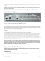
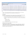
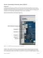
Tutorial - Introduction to LabScribe and the IX-ELVIS
Background
In addition to its prototyping capabilities, the iWorx Bioinstrumentation Breadboard for the National
Instruments Educational Laboratory Virtual Instrumentation Suite (IX-ELVIS) also provides users with
the ability to use physiological electrodes and transducers in the LabScribe software environment, and
to directly measure physiological parameters in a series of basic experiments.
Electrode and Transducer Connections (Figure 1-1)
Figure 1-1: IX-ELVIS electrode and transducer connections.
Channels 1 and 2 of the IX-ELVIS are set up as bioamplifiers and accept pin connectors such as those
on the snap electrodes used in measuring electrocardiograms (ECGs), electroencephalograms (EEGs),
and electromyograms (EMGs). The Channel 1 connectors are red (positive) and black (negative), while
Tutorial – IX-ELVIS
T-NI-1
the Channel 2 connectors are white (positive) and brown (negative). The green connector is a common
ground.
Channels 3 and 4 of the IX-ELVIS are transducer amplifiers. These accept mini-DIN connectors. The
gain is set by the transducer.
The IX-ELVIS board also includes two DAC stimulator outputs. These accept BNC connectors.
Rear Panel Connectors (Fig 1-2)
Figure 1-2: Back of IX-ELVIS showing USB and power jacks.
The USB connector is on the rear of the IX-ELVIS, as is the power cord jack and the power switch for
the unit. Both this power switch and the switch on the right side of the top of the unit must be switched
on in order to use the IX-ELVIS prototyping board.
Software
Use the supplied DVD to install the LabScribe software onto your computer.
Once installed, the LabScribe software usually resides in the iWorx folder in the Program Files folder
on the computer's hard drive. The software permits electrical signals to be displayed on the computer
screen in a format that resembles a traditional chart recorder. Each peripheral device may produce
signals of a different size and duration. You need to be able to adjust the software so that the signals are
the appropriate size and shape on the screen. This tutorial describes how to make these adjustments and
how to make simple measurements from traces.
In future experiments, you will open the software and find that many recording parameters have been
set for you. This permits you to collect data quickly and efficiently, making only minor adjustments to
obtain the best response. Over time, you may forget how to perform certain tasks; so, you can use this
tutorial or the LabScribe User Manual to refresh your memory.
Experiment 1: LabScribe2 - A Tutorial
LabScribe allows data to be accumulated, displayed and analyzed on a computer screen in a format
similar to a traditional chart recorder.
Equipment Setup
1. Place the IX-ELVIS unit on the bench, close to the computer.
Tutorial – IX-ELVIS
T-NI-2
2. Connect the IX-ELVIS to the computer with the supplied USB cable.
3. Insert the power plug into the rear of the IX-ELVIS and plug the transformer into the electrical
outlet. Turn on the power switches on the rear and on the upper right side of the top of the unit
and confirm that the LEDs are illuminated.
Start the Software
1. Click on the LabScribe icon on the Desktop, or click the Windows Start menu, click Programs
and open the iWorx folder and select LabScribe.
2. When the program opens, select Load Group from the Settings menu.
3. When the dialog box appears, select ELVISNI.iwxgrp and then click OK.
4. Click on the Settings menu again and select the Tutorial-LS2 settings file from the Tutorial
folder.
5. After a short time, LabScribe will appear on the computer screen as configured by the TutorialLS2 settings (Figure 1-3).
The LabScribe software has a few different views:
•
Main window: Record incoming signals and perform data analysis.
•
Analysis window: Perform data analysis.
•
XY Plot: Allows for plotting channel vs. channel data as in PV Loop Analysis.
•
FFT: Spectral analysis of data such as advanced EEG or HRV recordings.
•
Journal window: Type notes and insert recordings to create lab reports.
•
Marks: Review annotations entered during data acquisition.
•
Preview Mode: Examine incoming signals without recording them.
The Main window is displayed when LabScribe is first opened (Figure 1-3). Notice that each channel
has its own (white) recording area, with a title area at the upper left corner, AutoScale and add function
buttons, and the Value of the voltage at the upper right. Above the Voltage value is a Time value and the
Record button for starting and stopping the recording. The sampling Speed and the Display Time are
also located on the left. The Mark button and the comment entry line are located in the center of the
screen.
Tutorial – IX-ELVIS
T-NI-3
Figure 1-3: The LabScribe Main window (with computed rate channel added).
Connect the Hardware
The output from a pulse plethysmograph will be used as a signal source for this exercise.
1. Plug the pulse plethysmograph (PTN-104) into Channel 3's mini-DIN input (Figure 1-4).
2. Place the plethysmograph on the volar surface (where the fingerprints are located) of the distal
segment of the middle finger or the thumb, and wrap the Velcro strap around the end of the
finger to attach the unit firmly in place. Make sure it is not too tight.
Tutorial – IX-ELVIS
T-NI-4
Figure 1-4: IX-ELVIS with pulse plethysmograph connected.
Recording with LabScribe
The Signal
1. Click Record and record the finger pulse for at least 1 minute.
2. Click AutoScale in the Pulse channel (Channel 1) and see the rhythmic signal almost fill the
channel recording area.
3. Click Stop to halt recording; your recording may look like the top window in Figure 1-3.
The Screen Time
The default value for the time for a signal to cross the screen is 10 seconds. This value is displayed as
Display Time in the area above the Channel 1 title area. The Display Time can be changed by clicking
the display controls in the LabScribe toolbar (Figure 1-5).
To demonstrate the display controls:
1. Click the left icon (big single mountain – half display time) and notice that the trace spreads
out; the display time is now five seconds.
2. Click the right icon (small mountains – double display time) twice and see that the rhythmic
peaks get closer; the display time is now 20 seconds.
Tutorial – IX-ELVIS
T-NI-5
3. Click the left icon once to return to a 10-second display time.
Figure 1-5: The icons and functions in LabScribe.
The Sampling Rate
The default value for the number of samples taken per second is 200. This value is displayed above the
Channel 1 recording window. While this value is acceptable for most experiments, it can be changed by
selecting Preferences in the Edit menu and adjusting the sampling rate. Such a change does not alter the
screen display time.
Making Marks on a Record
Many experiments are divided into a series of exercises. It is convenient to annotate each exercise, so
that during subsequent review of your data file it is possible to determine what was done at any
particular stage during recording.
Entering Marks while Recording:
Marks can be entered “on-the-fly” while data are being recorded. Use the keyboard to type comments
on the line next to the Mark button. Press the Mark button, or the Enter key on the keyboard, and a
vertical line will be placed on the recording and that line will be associated with the comment typed on
the line. Try this:
1. Click Record.
2. Type “Mark#1” using the keyboard and notice that the words appear on the line to the right of
Mark button.
3. Press the Enter key on the keyboard and notice that:
•
the words disappear
•
a vertical line appears in the LabScribe window.
4. Type “Mark#2” and repeat step #3.
Tutorial – IX-ELVIS
T-NI-6
5. Repeat to enter a total of five different comments, pressing the Enter key after each.
6. Click Stop.
Entering marks when not recording:
When data have been recorded, two vertical lines or cursors appear on screen. These lines can be used
to make measurements such as V2-V1 and T2-T1. However, if you use the keyboard to type a comment
on the line next to the Marks button and press the Enter key, the comment will be entered in the lower
margin at the left cursor.
The last mark may be seen in the lower margin of the recording window.
This is helpful if you need to annotate the recording after the fact based on something observed within
the data file.
Saving a LabScribe File
It is wise to save work in any computer application and LabScribe is no exception:
1. Click on the File menu and select Save As.
When the Save As panel appears, type the name of the file. Choose a destination on the computer in
which to save the file. Click the Save button to save the file (as an *.iwxdata file).
Data Analysis of Your LabScribe File
Data analysis can be done in the either the Main or the Analysis window. Access to these windows can
be gained by clicking on the appropriate icon on the LabScribe toolbar (Figure 1-6).
Figure 1-6: The LabScribe icons in the toolbar.
Data Analysis in the Main Window
Navigating the Main Window
There are two ways to navigate around a data file in the Main window: the scroll bar, or the down
arrow to the left of the Marks button.
Scrolling
1. Move the cursor to the scroll bar in the lower margin of the Main window.
2. Click the arrows or move the slide to scroll the screen to the left or right. The typed marks
appear in the lower margin of the window.
Tutorial – IX-ELVIS
T-NI-7
Marks
1. Click the down arrow next to the Marks button. Once clicked, you will see a list of your typed
comments.
2. Click on one of the comments, and the software will automatically move to that section of
recorded data.
The comments associated with a mark can be moved vertically and placed anywhere on the recording
by clicking on the comment and dragging the mouse. Comments in a given view can be reset to the
lower margin by selecting Reset Marks using the down arrow to the left of the Marks button.
Figure 1-7: The cursor and display time icons in the LabScribe toolbar.
Making Measurements on the Main Window
Measurements are taken using the cursors. These are the vertical lines that address all channels and can
be called using one of the cursor icons (Figure 1-7) in the LabScribe toolbar.
Using a Single Cursor:
Click the 1-Cursor icon (single vertical bar). A vertical line appears over the recording window. Click
and drag the line to the left or right to make measurements of:
•
the absolute Time from the beginning of the trace, which is shown in the top right margin as
Time = .
•
the absolute Value of the voltage, which is displayed on the upper right margin of each channel
as Value = .
Using Two Cursors:
1. Click the 2-Cursor icon (two vertical bars). Two vertical lines appear over the recording
window (Figure 1-7).
2. Click and drag the lines left and right to display the difference in:
•
time between the positions of the two cursor lines. This difference is labeled as T2-T1 and is
shown in the top right margin.
•
voltage between the intersects of the two cursor lines on the trace. This difference is labeled
as V2-V1 and is shown on the upper right margin of each channel.
Tutorial – IX-ELVIS
T-NI-8
Figure 1-8: Cursors placed around the section of pulse recording selected for use in the Analysis
window. Note the Zoom Between Cursors button between the mountain icons.
The Journal
The Journal is a window that can be used as a notebook. Notes can be typed into the Journal, data and
traces can be copied and pasted into it, and the contents of the Journal can be printed.
•
Open the Journal by clicking the Journal icon (clipboard) on the LabScribe toolbar (Figure 1-6).
•
To transfer a recording to the Journal, use the Tools menu to select what you want copied to the
Journal:
•
Add title to Journal
•
Add all data to Journal
•
Add image to Journal
Return to the Main window by clicking on in the Journal icon again.
Data Analysis in the Analysis Window
Additional data analysis features are available through the Analysis window (Figure 1-9). Before the
Analysis window can be opened, you may wish to select a section of data in the Main window by
placing the two vertical cursors around the data of interest and clicking the Zoom Between Cursors
button on the LabScribe toolbar (Figure 1-7).
Tutorial – IX-ELVIS
T-NI-9
Figure 1-9: A finger pulse recording in the Analysis window.
To select the data to be displayed in the Analysis window:
1. Click and drag the two vertical cursors left and right so that the section of the recording to be
used in the Analysis window is between the cursors. Place the cursors so that 5 complete pulse
cycles are selected.
2. Click the Zoom Between Cursors button (between the mountain peaks).
3. Open the Analysis window by clicking the Analysis icon on the LabScribe toolbar (Figure 1-7).
Channel Display in the Analysis Window
In this window, the recordings from all available channels are displayed under one another.
If two or more channels are displayed in the Analysis window, the traces can be stacked or
superimposed over each other by clicking the Stacked box on the lower left margin of the Analysis
window.
Screen Display in the Analysis Window
The display time in the Analysis window can be changed in the same manner it is in the Main window.
Clicking on the Display Time icons (mountains) will double or half the display time for each click
(Figure 1-4). The trace can also be scrolled horizontally by using the arrows or slider on the lower
margin of the window.
Data Values in the Analysis Window
Data functions and values for all the channels are displayed across the upper margin of each channel in
the Analysis window. The accuracy of the values (number of decimal places) can be set by using the
Edit > Preferences > Options menu and changing the Data Display Precision.
The functions displayed across the top margins of the channel in the Analysis window can be added by
clicking on the add function button. The titles of the functions and the matching data can be copied into
Tutorial – IX-ELVIS
T-NI-10
the Journal by clicking the Tools menu or clicking the down arrow to the left of the channel name and
selecting either the Add Titles to Journal or Add Data to Journal item from this menu.
Sample Data Measurement
Determine the subject’s heart rate from the finger pulse data displayed in the Analysis window. Also,
copy the trace displayed in the Analysis window to the Journal:
1. Move the cursors so each cursor is located on a peak of an adjacent finger pulse. The time
between the cursors is the period of the pulse cycle.
2. Select Title and T2-T1 from the add functions list.
3. Click the Journal icon on the toolbar (Figure 1-7).and then click the down arrow to the left of
the Pulse channel. Select Add Title to Journal and Add Ch Data to Journal to transfer the title of
the channel (Pulse) and the value measured (T2-T1) to the Journal.
4. Click Tools and Add Image to Journal. The trace in the Analysis window will now appear in the
Journal.
5. Calculate the subject’s heart rate by dividing 60 (as in 60 sec/min) by T2-T1 (secs/heart beat).
T2-T1, is the period of each heart beat cycle.
6. Return to the Main window by clicking the Main window icon on the toolbar (Figure 1-7).
Channel Features
Additional features for each channel are available from the add functions menu in the Main window.
These calculated channels can all be set up prior to data collection. Some of the functions available
include: rates, integrals, filters, units conversions, scaling, and mathematical manipulations.
To demonstrate the usefulness of one of these functions, integrate the finger pulse signal to display the
heart rate from the finger pulse:
1. On Channel 1 (Pulse) click the add function button and choose Periodic > Rate. When the new
window opens, just click OK to set the new channel features.
•
Note the 2 blue horizontal cursors shown in the popup window. These can be adjusted to
make sure they are intersecting the peaks of the pulse waves only. Just click and drag them
to the correct location if they need to be moved.
2. If necessary, click AutoScale for new Rate calculated channel to display the Heart Rate from the
pulse data on the screen.
3. Click the 2-Cursor icon (Figure 1-8). Two vertical lines appear over the Main window.
4. Drag the cursors to the left and to the right to select 5 pulse cycles between the two blue lines.
Click the Zoom Between Cursors button.
5. Open the Analysis window by clicking the Analysis icon on the LabScribe toolbar (Figure 1-7).
6. Make the following measurements from recordings displayed in the Analysis window (Figure
1-10) using the Title, V2-V1, T2-T1, and Mean functions listed in the add functions list in the
Analysis window:
Tutorial – IX-ELVIS
T-NI-11
•
Amplitude of the Pulse Wave: Place the cursors on the trough and the peak of a pulse wave
and look at the Title and V2-V1 on the Pulse channel. This value is measured in volts.
•
Period of the Pulse Wave: Place the cursors on the peaks of two adjacent pulse waves. The
value for T2-T1 is the pulse period, which can be used to mathematically calculate the heart
rate.
•
Mean Heart Rate over a period of time: Use the double display time icon to show the entire
recording on screen. The icon may need to be clicked more than once. Once the entire
recording is shown, place the cursors on either end of the recording. The value for Mean is
the heart rate for the subject over the period of time shown in T2-T1.
Figure 1-10:Finger pulse (upper trace) and the heart rate (lower trace).
In the future, you will use functions available in the Analysis window to determine values for arterial
blood pressure, relative blood flow, heart rate, lung volumes, nerve conduction velocity, and more.
Tutorial – IX-ELVIS
T-NI-12