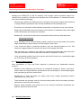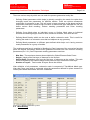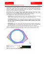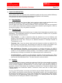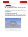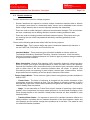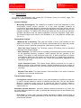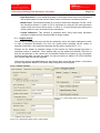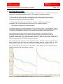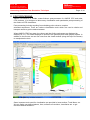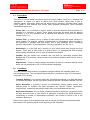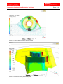
1
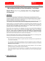
FH D
Fachhochschule Düsseldorf
University of Applied Sciences
FMDauto
Institut für Produktentwicklung
und Innovation
Harvesting-Combine-Flow Simulation Technique
Page 1/14
Harvesting-Combine-Flow Simulation Technique
Madhur Bhaiya, Prof. Dr.-Ing. Andreas Jahr, B.Eng. Holger Happel
FH Düsseldorf
1
ABSTRACT
CFX 11.0 is a Computational Fluid Dynamics (CFD) program for simulating the behavior
of systems involving fluid flow, heat transfer, and other related physical processes. It works by
solving the equations of fluid flow (in a special form) over a region of interest, with specified
(known) conditions on the boundary of that region.
This tool is used here to analyse the straw cutter which is used to comminute the straw which
is left standing in the field after stripper header has stripped the grains from the crops.
Stripper Header is a new technique different to conventional harvester machines and it is still
under development and testing. It works on the principle in which grains are first stripped off
from the head of the standing crop which helps in much reduced intake freeing up the
separation systems to handle a larger volume of grains.
But with this, the new problem of the disposal of the long, uncut straw left after stripping of
grains arose. So a straw cutter is used after the stripper header stage in this Combine
Harvester, where the rotor is equipped with pressed steel blades and rotates towards the
crop, i.e., it cuts and lifts the straw over the top. This technique is environment friendly
because previously farmers would have to burn the long, uncut straw standing in the fields
while in this case mulched straw can be used for min-till systems.
This rotor based straw cutting machine is analysed here which helps us in increasing power
efficiency and comminution rate and quality of cut straw particles.
Here fluid flow simulation has been preferred over particle simulation:
-
CFX 10.0 tool is not very effective for particle simulation techniques and computation time
is increased considerably.
-
It’s very hard to realize particle simulation in CFX 10.0 because we have to define size
and properties of each particle and besides this wall conditions would have to be defined
differently for every boundary.
-
Besides this, it’s hard to realize cutting effect with straw particles in CFX 10.0 which
otherwise would be comminuted in real life conditions.
-
The results obtained from fluid simulation are validated using experimental results and
found to be nearly the same which clearly contradicts any need of performing particle
simulation.
2 MESH GENERATION
FH D
Fachhochschule Düsseldorf
University of Applied Sciences
Harvesting-Combine-Flow Simulation Technique
FMDauto
Institut für Produktentwicklung
und Innovation
Page 2/14
Meshing tool ICEM-CFD is used for meshing. This involves various important steps to be
realized during meshing. Geometry was imported from CAD software i.e. Autodesk Inventor
and it was modified accordingly.
-
Whole body is defined into different parts by grouping of geometric entities which allows us
to assign different parameters and boundary conditions on the individual parts.
-
Even these can be used to define different parameters on individual curves and surfaces.
-
Using these prescribed points and surfaces, the locations of tetrahedral nodes and edges
in the critical areas of the mesh are controlled.
-
Besides this, various factors like mesh smoothness and fineness are dealt with ease.
Repairing Geometry
-
“Build Topology” tool is executed which creates a series of curves and points from surface
edges depending on the proximity of surface edges to each other.
-
If the curves are within a geometric tolerance, they are merged together as one. This
tolerance is approximately one-tenth of the size of the average mesh size.
-
This tool helps us to diagnose the model for geometrical problems like gaps and holes.
They take automatic colours to show their association to adjacent surfaces.
-
If any geometrical problem found, then various tools like fill, blend, trim, match/stitch edges
etc. are used to fix these problems.
2.2
Meshing Requirements
Here combination of Tetra and Prism elements is preferred over Hexahedral element
because:
-
Despite of more efficiency and accuracy of hexahedral meshes (in terms of grid size),
these meshes are highly difficult to generate and time consumption is considerably higher
than generating a tet-prism combo mesh.
-
Combination of Tetra and Prism can easily mesh even complex geometries without
affecting accuracy very much.
-
Tetra elements are generally used for volume meshing while closer to boundary prismatic
elements are used for better meshing.
-
Regions where boundary layer effects are to be resolved, sometimes excessively fine
grids are needed close to the wall.
2.3
Meshing Parameters
FH D
Fachhochschule Düsseldorf
University of Applied Sciences
FMDauto
Institut für Produktentwicklung
und Innovation
Harvesting-Combine-Flow Simulation Technique
Page 3/14
There are various ways by which we can mesh the present geometrical entity like:
-
Defining Global parameters which helps in globally controlling the mesh size rather than
changing mesh size parameters for different entities. There are various refinements
techniques for elements in gap. This will result in larger elements on flat planar surfaces
and smaller elements in areas of high curvature or within small gaps. Besides this, we can
define various Shell meshing, Volume meshing parameters and Prism meshing
parameters.
-
Defining Curve Mesh sizes on individual curves or Surface Mesh sizes on individual
surfaces and defining height, minimum size, maximum deviation, tetra size ratio etc.
-
Defining Mesh Density which can be used to define volumetric mesh. This is useful for
refining the mesh in a volumetric zone that isn't adjacent to any geometry
-
Defining Mesh parameters on different parts defined which helps us in having common
mesh parameters for a group of entities.
The technique used here in meshing is ‘Meshing by Parts’ because of the convenient fact that
parts are defined accordingly where some geometrical entities can have common meshing
parameters.(Pic 2.3.1) Some important meshing parameters used are:
-
Max Size: The maximum element size multiplied by Global Element Scale Factor.
Height: Height of the first layer of elements on the surface.
Height Ratio: Expansion ratio from the first layer of elements on the surface. This ratio
will be multiplied by the element height of the previous layer to define the next layer.
Number of Layers: Total number of layers above the surface.
After definition of all parameters, volumetric mesh is computed of Tetra/Mixed Mesh type.
After that Prism type mesh is computed using the parameters defined for prism elements in
certain parts where wall effects are to be considered.
Picture 2.3.1: Meshing Parameters by Parts.
2.4
Mesh Editing
FH D
Fachhochschule Düsseldorf
University of Applied Sciences
Harvesting-Combine-Flow Simulation Technique
FMDauto
Institut für Produktentwicklung
und Innovation
Page 4/14
Mesh editing is required for improving its quality. For Hexa mesh, the ideal element will be a
cuboid, and in case of Tetra mesh, the ideal element is a tetra with equal side lengths and
equilateral triangles for each face. Edit Mesh has the tools required for modifying all those
elements which are not similar to the ideal element.
Mesh Editing tools are mostly automatic in ICEM. Three factors are taken care of while
editing meshes which are Quality, Aspect Ratio and Determinant. Quality having value
more than 0.3 is considered to be good and same goes for other two factors.
Some important tools used for improving these mesh factors are:
-
Check Mesh: Here mesh is checked for various errors like Duplicate Element, Uncovered
Faces, Missing Internal Faces, Periodic Problems, and Hanging Elements etc.
-
Smooth Mesh Globally: This automatically improves the quality of the mesh depending
on various kinds of smoothening algorithm available in ICEM for different kind of mesh
elements. Following parameters to be looked upon like Number of Iterations, Up to Quality
and Quality factor.
-
Repair Mesh: There are various mesh repairing tools used for manually editing parts of
the mesh which are not of good quality. Some of the relevant tools are Remesh Bad
Elements, Find/Close Holes in Mesh, Stitch Edges, and Smooth Surface Mesh etc.
After this, being satisfied with mesh quality and other factors like fineness of mesh, mesh is
ready to be imported in CFX-Pre as mesh files (*.msh & *.gtm) for simulations (Pic 2.4.1).
Picture 2.4.1: Meshed geometry with quality histograms.
FH D
Fachhochschule Düsseldorf
University of Applied Sciences
Harvesting-Combine-Flow Simulation Technique
FMDauto
Institut für Produktentwicklung
und Innovation
Page 5/14
3 PHYSICS DEFINITION
Here meshes which are imported and assembled together as they were meshed differently
and after that basic physical models and settings are applied on the assembly.
This procedure is done in following various steps:
3.1
Importing Mesh
Meshes are imported using ‘Import Mesh’ option and then various mesh transformation tools
are used like translation, rotation, scaling etc. to assemble meshes together.
We can import more than one mesh per ANSYS CFX-Pre simulation. After we have imported
all our meshes and created all our domains, the domains should be joined together, either by
gluing them together, or by using domain interfaces.
3.2
Simulation Type
Here it is decided whether the simulation type is steady (time independent) or transient (time
dependent). Time dependent behavior for transient simulations in ANSYS CFX is specified
through following Transient Scheme:
-
Time Duration: In order to determine when the transient run is to be finished, total
duration of the simulation in real time is mentioned here. It can be set to any one of these
parameters like Total Time, Times per run, Maximum Number of Timesteps, Number of
Timesteps per run etc.
-
Timesteps List: Here we set the actual real time intervals at which the ANSYS CFXSolver solves for the flow field. The timesteps we select are needed to be based on the
time scale of the transient behavior that we want to resolve in our flow simulation.
-
Max. Iterations per Timestep: At each timestep in a transient simulation, the ANSYS
CFX-Solver performs several coefficient iterations or loops, either to a specified maximum
number or to the predefined residual tolerance. The maximum number of iterations per
timestep may not always be reached if the residual target level is achieved first.
-
Transient Scheme: It defines the discretization algorithm for the transient term. There
are two schemes available in transient simulation, which are First Order Backward Euler
and Second Order Backward Euler. The latter scheme is used as default.
3.3
Domains
Domains are regions of space in which the equations of fluid flow or heat transfer are solved.
Here we define the type of region whether fluid, solid or porous. We can select varieties of
fluids and solids available in the Materials list, or we can create a new material by defining its
properties. Various Fluid Models are available for definition like Turbulence Models, Heat
Transfer Models and Combustion Models. Turbulence model used here is Shear Stress
Transport (SST).
For any given CFD problem, more than one domain may be defined. Each time we create or
edit a domain, the physical models (fluid lists, heat transfer models, etc.) are applied across
all domains of the same type (e.g., fluid or solid). Besides this, Domain Motion is also defined.
Each domain can be independently stationary or rotating. For rotating domains, the angular
velocity and axis of rotating are defined for each domain.
FH D
Fachhochschule Düsseldorf
University of Applied Sciences
Harvesting-Combine-Flow Simulation Technique
3.4
FMDauto
Institut für Produktentwicklung
und Innovation
Page 6/14
Boundary Conditions
Boundary Conditions are to be applied on all the bounding region of our domains (Pic 3.4.1).
Following Boundary types are available in CFX.
-
Inlet: Fluid flowing into domain. There are many different types of inlet boundary
condition combinations for the mass and momentum equations. Basically, it can be set
into two different parameters, Subsonic and Supersonic.
-
Outlet: Fluid flowing out of domain. The hydrodynamic boundary condition specification
(that is, those for mass and momentum) for a subsonic outlet involves some constraint on
the boundary static pressure, velocity or mass flow. It can also be set into two parameters,
Subsonic and Supersonic.
-
Opening: Fluid can simultaneously flow both in and out of the domain. This is not
available for domain with more than one fluid present.
-
Wall: Impenetrable boundary to fluid flow. Walls allow the permeation of heat and
additional variables into and out of the domain through the setting of flux and fixed value
conditions at wall boundaries. There are three options for the influence of a wall boundary
on the flow, namely, No Slip, Free Slip and Counter Rotating Wall.
-
Symmetry: A plane of both geometric and flow symmetry.
Picture 3.4.1: Mesh Assembly with applied boundary conditions.
FH D
Fachhochschule Düsseldorf
University of Applied Sciences
Harvesting-Combine-Flow Simulation Technique
3.5
FMDauto
Institut für Produktentwicklung
und Innovation
Page 7/14
Domain Interfaces
Domain interfaces are used for multiple purposes:
-
Domain Interfaces are required to connect multiple unmatched meshes within a domain
(for example, when there is a hexahedral mesh volume and a tetrahedral mesh volume
within a single domain) and to connect separate domains and assemblies.
- These are used to model changes in reference frame between domains. This occurs when
we have a stationary and a rotating domain or domains rotating at different rates.
-
These are used for creating periodic interfaces between regions. This occurs when you
are reducing the size of the computational domain by assuming periodicity in the
simulation.
These are the following parameters which fulfils the above purposes:
-
Interface Type: This is used to define the type of connection between two domains. It
can be Fluid Fluid, Fluid Solid, and Fluid Porous etc.
-
Interface Models: There are three types of models available to choose, which are
Translational Periodicity, Rotational Periodicity, General Connection. In this simulation
General Connection is preferred because it is useful to apply a pressure change condition
to a general domain interface.
-
Mesh Connection: General Grid Interface (GGI) connection method is used even when
there is a direct (one-to-one) correspondence in nodes on either side of the interface.
General Grid Interface (GGI) connections refer to the class of grid connections where the
grid on either side of the two connected surfaces does not match. In general, GGI
connections permit non-matching of node location, element type, surface extent, surface
shape and even non-matching of the flow physics across the connection.
- Frame Change Model: There are three types of frame change/mixing models available in
ANSYS CFX:
- Frozen Rotor: The frame of reference is changed but the relative orientation of the
components across the interface is fixed. The two frames of reference connect in such a
way that they each have a fixed relative position throughout the calculation. This model is
used in Steady State simulations.
- Stage: It’s an alternative to Frozen Rotor model. Instead of assuming a fixed relative
position of the components, the stage model performs a circumferential averaging of the
fluxes through bands on the interface. Steady state solutions are then obtained in each
reference frame.
- Transient Rotor Stator: It’s important to account for transient interaction effects at a
sliding interface. It predicts the true transient interaction of the flow between a stator and
rotor passage as rotor blades change there positions as in real time. This model is used
for transient simulation problems.
FH D
Fachhochschule Düsseldorf
University of Applied Sciences
Harvesting-Combine-Flow Simulation Technique
3.6
FMDauto
Institut für Produktentwicklung
und Innovation
Page 8/14
Solver Control
It is used to set parameters that control the CFX-Solver during the solution stage. The
settings are divided into three classes:
-
Common Settings:
-
-
Monitoring Convergence: The residual is a measure of the local imbalance of each
conservative control volume equation. It is the most important measure of
convergence as it relates directly to whether the equations have been solved. We can
select to use RMS (Root Mean Square) or MAX (Maximum) normalized values of the
equation residuals. The ANSYS CFX-Solver will terminate the run when the equation
residuals calculated using the method specified is below the Residual Target value.
The Residual target value used in this simulation is 1e-4 with RMS as residual type
(Pic 3.6.1).
Steady State Settings:
-
Maximum No of Iterations: This sets the number of outer loop iterations for the
ANSYS CFX-Solver. The ANSYS CFX-Solver will terminate the run after this number
of iterations, even if specified convergence criteria have not been reached.
-
Fluid Time Scale Control: The Timescale used by CFX-Solver can be controlled
using one of the three methods:
- Auto Timescale: This option uses an internally calculated physical time scale based
on the specified boundary conditions, initial guesses and the geometry of the
domain. This option is used as default option as it is often conservative to ensure
convergence. While using this option for fluid domains in a steady-state simulation,
the Length Scale Option may also be set. These are conservative, aggressive and
specified length scale.
- Local Timescale Factor: This option allows different timescale to be used in
different regions of the calculation domain. Smaller timescales are to the regions of
flow where local timescale is very short and large where local timescale is relatively
very large.
- Physical Time Scale: This option allows a fixed timescale to be used for selected
equations over the entire flow domain.
-
Transient State Settings:
- Convergence Control: Default value of 10 is used in Maximum Coefficient Loops; this
is used to set the maximum number of iterations per time step. We can also enable
Minimum Coefficient Loops option as it restricts the solver to perform atleast a
minimum number of iterations whether desired convergence is achieved or not. Its
default value is 1.
-
Advection Scheme Selection: Advection means transport phenomenon in a fluid. We
can select different schemes in order to calculate the advection terms in the discrete finite
volume equations.
- First Order: It is First order accurate scheme equivalent to specify a blend factor of
0.0. It gives the most robust performance of the Solver but it suffers from the problem
of Numerical Diffusion.
FH D
Fachhochschule Düsseldorf
University of Applied Sciences
Harvesting-Combine-Flow Simulation Technique
FMDauto
Institut für Produktentwicklung
und Innovation
Page 9/14
- High Resolution: It’s the preferred setting; in this blend factor values vary throughout
the domain based on local solution field in order to enforce a boundness criterion.
- Blend Factor: This selection allows us to select a blend factor between 0.0 and 1.0 for
the advection scheme. A value of 0.0 is equivalent to using the first order advection
scheme and is the most robust option. A value of 1.0 uses second order differencing
scheme which is more accurate but less robustness.
- Central Difference: This scheme is available when using large eddy simulation
turbulence models and it’s recommended for those models.
3.7
Output Control
This is used to manage the way how files are written by solver. All default settings are used,
in case of transient simulations, the user can control which variables will be written to
transient result files (*.res) and how frequently the files will be created (Pic 3.7.1).
Results can be written at particular stages of the solution by writing backup files after a
specified number of iterations. These backup files can be loaded into ANSYS CFX-Post so
that the development of the results can be examined before the solution is fully converged.
Particle tracking data can also be written for post processing in ANSYS CFX-Post. Besides
this, surface data can also be exported.
After this all settings and parameters are well chosen then solver files are written (*.def) which
are then exported to ANSYS CFX-Solver where equations are calculated.
Picture 3.7.1: Basic Steady State Output Control
Settings
Picture 3.6.1: Basic Steady State Solver Control settings
FH D
Fachhochschule Düsseldorf
University of Applied Sciences
FMDauto
Institut für Produktentwicklung
und Innovation
Harvesting-Combine-Flow Simulation Technique
Page 10/14
4 SOLVING EQUATIONS
The component that solves the CFD problem is called the Solver. It produces the required
results in a non-interactive/batch process. A CFD problem is solved as follows:
- The partial differential equations are integrated over all the control volumes in the
region of interest. This is equivalent to applying a basic conservation law (for example,
for mass or momentum) to each control volume.
- These integral equations are converted to a system of algebraic equations by
generating a set of approximations for the terms in the integral equations.
-
The algebraic equations are solved iteratively.
An iterative approach is required because of the non-linear nature of the equations, and as
the solution approaches the exact solution, it is said to converge. For each iteration, an error,
or residual, is reported as a measure of the overall conservation of the flow properties.
How close the final solution is to the exact solution depends on a number of factors,
including the size and shape of the control volumes and the size of the final residuals.
Complex physical processes, such as combustion and turbulence, are often modeled using
empirical relationships. The approximations inherent in these models also contribute to
differences between the CFD solution and the real flow.
The solution process requires no user interaction and is, therefore, usually carried out as a
batch process. One can also use parallel processing features of the solver for faster
processing. Besides this, it is also used to monitor residuals and convergence (Pic 4.1).
The solver produces a results file (*.res) which is then passed to the post-processor for
further processing and interpretation of results.
Picture 4.1: Monitoring Mass-Momentum and Turbulence (KO) residuals for steady state solution
FH D
Fachhochschule Düsseldorf
University of Applied Sciences
Harvesting-Combine-Flow Simulation Technique
FMDauto
Institut für Produktentwicklung
und Innovation
Page 11/14
5 POST PROCESSING
ANSYS CFX-Post is a flexible, state-of-the-art post-processor for ANSYS CFX and other
CFX products. It is designed to allow easy visualization and quantitative post-processing of
the results of CFD simulations.
Post-processing includes anything from obtaining point values to complex
animated sequences. There are various visualisation tools which are used to obtain and
interpret results to get the desired answer.
When ANSYS CFX-Post starts, the viewer and the Outline workspace are displayed by
default (Pic 5.1). The viewer displays an outline of the geometry and other graphic objects. In
addition to the mouse, we can use icons from the viewer toolbar (along the top of the viewer)
to manipulate the view.
Picture 5.1: Sample Ansys CFX-Post Interface
Some important tools used for visualisation are provided in Insert toolbar, Tools Menu, etc.
We can make user defined planes, lines, surfaces of revolution, isosurfaces etc. to get
results at desired locations.
FH D
Fachhochschule Düsseldorf
University of Applied Sciences
Harvesting-Combine-Flow Simulation Technique
5.1
FMDauto
Institut für Produktentwicklung
und Innovation
Page 12/14
Insert Menu
This menu is used to create new objects (such as locators, tables, charts, etc.), variables and
expressions. A locator is a place or object upon which another object uses to plot or
calculate values. With every object we can adjust colour, geometry, reduction factor, scale
(local, global or user defined) and various other graphical parameters. Some important
visualisation objects are:
-
Vector Plot: It is a collection of vectors drawn to show the direction and magnitude of a
variable on a collection of points. These points are known as seeds, and are defined
allocation. It is a very important tool to visualise flow direction of the fluid at different
locations.(Pic 5.1.1)
-
Contour Plot: A contour plot is a series of lines linking points with equal values of a
given variable. For example, contours of height exist on geographical maps and give us
an impression of gradient and land shape. This is very important tool in visualising
pressure magnitudes, YPlus magnitudes, Velocity magnitudes, etc.(Pic 5.1.2)
-
Streamlines: It is the path that a particle of zero mass would take through the fluid
domain. These start at each node on a given locator. It is assumed that flow is steady
while creating streamlines, even in case of transient simulations.
-
Variable: We can define new variables and use them for calculating desired data.
Besides this CFX provides a large number of pre defined variables which can be used in
expressions.
-
Expressions: It can be used to define expressions in order to calculate desired values
which are not predefined in CEL (CFX Expression Language).
5.2
Tools Menu
The tools window offers access to quantitative analysis utilities, the animation editor and
the timestep selector. The Command Editor dialog box is available to enter CFX Command
Language (CCL) directly.
-
Timestep Selector: For transient results file, this dialog box allows us to load the results
for different timesteps. We can use various features like Add Timesteps, Multiple Files etc.
-
Quick Animation: It provides a means to automatically sweep objects across their
defined range to visualise the data throughout the domain. Planes, Isosurfaces,
turbosurfaces, streamlines and particle tracks may all be animated with this tool.
-
KeyFrame Animation: We can make animations based on keyframes. Keyframes define
the start and end points of each section of animation. Keyframes are linked together by
interpolating a number of intermediate keyframes, the number of which is set in the
Animation dialog box.
These are the some of the important tools used to analyse and interpret the desired results
and answer to the question posed at the beginning of the simulation.
FH D
Fachhochschule Düsseldorf
University of Applied Sciences
Harvesting-Combine-Flow Simulation Technique
Picture 5.1.1: Vector plot of Velocity in Stationary Frame
Picture 5.1.2: Pressure contour plot of Blade profile
FMDauto
Institut für Produktentwicklung
und Innovation
Page 13/14
FH D
Fachhochschule Düsseldorf
University of Applied Sciences
FMDauto
Institut für Produktentwicklung
und Innovation
Harvesting-Combine-Flow Simulation Technique
Page 14/14
6 CONCLUSION
CFX proves to be a quite flexible software for fluid simulations. Besides having limitations
with particle simulation technique, it is good for fluid simulation. These steps are quite vital
for any simulation and the experimental results are validated with simulation results.
Tetra-Prism combo mesh is preferred over Hexa elements considering time factor and ICEM
has quite efficient smoothening algorithms to improve the quality of the mesh.
Pre settings are different in case of Solver control and Output control for Steady state
simulation and transient state simulation, while it’s same in rest parameters.
Post processor tools are very important to get the desired results and answer to the posed
question for which simulation is done. There are various effective graphical tools to get an
insight of the fluid flow process in the desired domain.
7 REFERENCES
-
8
ANSYS CFX Release 11.0 User Manual, Released on December 2006
AUTHORS:
MADHUR BHAIYA ([email protected])
Cand. B. Tech. in Mechanical Engineering
Prof. Dr.-Ing. Andreas Jahr ([email protected])
Professor for Mechanical Design and Mechanics
B.Eng. Holger Happel ([email protected])
Scientific Coworker
The authors have been members of FMDauto – Institute of Product Design and
Innovation.
Die Autoren waren Mitglieder von FMDAUTO - Institut für Produktentwicklung und
Innovation der FH Düsseldorf (www.fmdauto.de).