Download Program Tutorial

AFMG SysTune
Developed by
AFMG Ahnert Feistel Media Group
The creators of EASE and EASERA
www.AFMG.eu
Software Manual, Rev. 5, May 2014
Copyright © 2006-2014 AFMG Technologies GmbH
- Contents
Contents
Contents ...................................................................................................................................... 2
Preface......................................................................................................................................... 6
General Program Information ..................................................................................................... 7
SysTune's capabilities include: ........................................................................................... 7
The Pro version of SysTune adds the following features: .................................................. 7
Equipment Requirements .................................................................................................... 8
Software Support ................................................................................................................ 8
SysTune Installation and Licencing ................................................................................................ 9
1. Installation Instructions ........................................................................................................... 9
1.1. Microsoft .NET Framework 2.0....................................................................................... 9
1.2. SysTune Startup ............................................................................................................... 9
AFMG SysTune .................................................................................................................. 9
AFMG Licence Manager .................................................................................................... 9
NGINX Webserver ............................................................................................................. 9
1.3. SysTune User Files .......................................................................................................... 9
1.4. Licencing the Software .................................................................................................... 9
2. Licencing Instructions ........................................................................................................... 10
2.1. Online Licencing ............................................................................................................ 10
2.2. Licencing by File ........................................................................................................... 10
Reference File ................................................................................................................... 10
Licence File ....................................................................................................................... 10
2.3. AFMG Licence Manager Program ................................................................................ 11
Licence Status ................................................................................................................... 11
Online Licencing ............................................................................................................... 12
Licencing by File – Licence Tab ...................................................................................... 13
Licencing by File – Terminate Tab ................................................................................... 14
Licencing by File – Import / Export Tab .......................................................................... 15
Proxy Server Configuration Window ............................................................................... 15
Program Tutorial ........................................................................................................................... 16
1. Introduction ........................................................................................................................... 16
Preface................................................................................................................................... 16
Starting the Software............................................................................................................. 16
Screen Layout ....................................................................................................................... 17
2. Measurements with a Single Input Channel ......................................................................... 19
Selecting the Input Channel .............................................................................................. 19
2.1. Time Signal .................................................................................................................... 20
Calibrating an Input Channel ............................................................................................ 21
Adjusting the View Limits ................................................................................................ 25
Summary ........................................................................................................................... 27
2.2. Input Spectrum ............................................................................................................... 28
Choosing the FFT Size...................................................................................................... 33
Averaging over Time ........................................................................................................ 34
Checking the Calibration .................................................................................................. 35
Summary ........................................................................................................................... 37
2.3. Spectrogram ................................................................................................................... 37
2
- Contents
Synchronizing Views ........................................................................................................ 40
Storing and Recalling Views ............................................................................................ 40
Summary ........................................................................................................................... 41
3. Measurements with an Excitation Signal .............................................................................. 42
3.1. Excitation Signal ............................................................................................................ 42
Choosing a Stimulus Signal .............................................................................................. 42
Activating the Output Channel ......................................................................................... 45
Frequency Response Measurements ................................................................................. 45
Summary ........................................................................................................................... 46
3.2. Capturing and Comparing Measurements ..................................................................... 47
Overlay Properties ............................................................................................................ 48
Active Curve ..................................................................................................................... 50
Saving, Removing and Loading Overlays ........................................................................ 51
Averaging Measurements ................................................................................................. 52
Adding Cursors ................................................................................................................. 54
Displaying Harmonics ...................................................................................................... 58
Summary ........................................................................................................................... 58
4. Dual-FFT Measurements ...................................................................................................... 59
Setup with Internal Reference ........................................................................................... 59
Setup with External Reference.......................................................................................... 60
4.1. Transfer Function Measurements .................................................................................. 61
Measuring Principles ........................................................................................................ 61
Computation of the Transfer Function .............................................................................. 62
Real-Time Deconvolution (RTD™) ................................................................................. 63
Transfer Function in SysTune ........................................................................................... 64
Example ............................................................................................................................ 65
Summary ........................................................................................................................... 67
4.2. Impulse Response .......................................................................................................... 67
Trouble-Shooting .............................................................................................................. 69
Impulse Response Measurements ..................................................................................... 70
Delay Alignment of Loudspeakers ................................................................................... 73
Saving Impulse Responses ................................................................................................ 75
Level Meters ..................................................................................................................... 76
Summary ........................................................................................................................... 77
4.3. ETC ................................................................................................................................ 77
Analyzing Reflections ....................................................................................................... 78
Summary ........................................................................................................................... 79
4.4. Magnitude ...................................................................................................................... 80
Relationship between Transfer Function and Impulse Response ..................................... 80
Magnitude of the Transfer Function ................................................................................. 80
Coherence and IR Stability ............................................................................................... 83
Adjusting the Gain Offset ................................................................................................. 85
Averaging Transfer Functions .......................................................................................... 86
Exporting Graph Data ....................................................................................................... 89
Introduction to Windowing ............................................................................................... 89
Windowing in SysTune..................................................................................................... 90
Windowing Options and Options Window ....................................................................... 94
TFC Window™ .............................................................................................................. 101
3
- Contents
Processing Windowed Data ............................................................................................ 103
Summary ......................................................................................................................... 103
4.5. Phase ............................................................................................................................ 104
Meaning of Phase Data ................................................................................................... 104
Using the Phase Graph for Delay Alignment ................................................................. 105
Smoothing and Wrapping Phase ..................................................................................... 111
5. Further Measurements ........................................................................................................ 113
5.1. Noise Level Measurements .......................................................................................... 113
Noise Criteria NC ........................................................................................................... 113
Additional Noise Criteria RNC, NR, RC Mark II .......................................................... 114
Summary ......................................................................................................................... 115
5.2. SPL and LEQ Measurements ....................................................................................... 115
SPL and LEQ Monitor .................................................................................................... 115
Histo Graph ..................................................................................................................... 117
Health Regulations Plug-In ............................................................................................. 119
Summary ......................................................................................................................... 123
5.3. Measurements using Multiple Signal Channels ........................................................... 123
Changing Soundcard and Driver ..................................................................................... 124
Status Bar ........................................................................................................................ 125
Multi-Channel Measurements ......................................................................................... 126
Mapping Input Channels ................................................................................................. 127
5.4. Reverberation Time and Speech Intelligibility ............................................................ 128
Reverberation Time ........................................................................................................ 128
Speech Intelligibility ....................................................................................................... 134
Extended Speech Intelligibility Measurements .............................................................. 135
Summary ......................................................................................................................... 137
5.5. Measurements using Speech and Music Signals ......................................................... 137
Basic Noise Suppression Tools ....................................................................................... 139
Spectrally Selective Accumulation (SSATM) Filter ........................................................ 140
Advanced Settings for SSA Filter ................................................................................... 142
5.6. Virtual Equalizer (Virtual EQ)..................................................................................... 144
Using the Virtual EQ ...................................................................................................... 144
Locking Overlays ............................................................................................................ 148
Advanced EQ .................................................................................................................. 148
Summary ......................................................................................................................... 151
5.7. Delay Analysis ............................................................................................................. 151
Functional Overview ....................................................................................................... 152
Using Delay Analysis ..................................................................................................... 155
Summary ......................................................................................................................... 157
5.8. Web Interface ............................................................................................................... 157
Using the Web Interface ................................................................................................. 158
Summary ......................................................................................................................... 162
5.9. AUBION X.8 Input Gain Compensation ..................................................................... 162
5.10. Plug-Ins ...................................................................................................................... 164
Using a DSP Plug-In ....................................................................................................... 164
R1 Integration – Importing/Exporting Filter Settings ..................................................... 165
Normalization Plug-In .................................................................................................... 167
Summary ......................................................................................................................... 169
4
- Preface
5.11. Lake Controller Integration........................................................................................ 170
5.12. Impedance .................................................................................................................. 176
5.13. Off-Line Analysis ...................................................................................................... 178
6. Additional Topics................................................................................................................ 179
6.1. Menu Structure............................................................................................................. 179
6.2. Keyboard Short Cuts .................................................................................................... 181
6.3. View Limits and Graph Formatting ............................................................................. 182
Default and Current View Limits ................................................................................... 183
Graph Layout .................................................................................................................. 184
Curve Properties.............................................................................................................. 185
6.4. Trouble Shooting ......................................................................................................... 186
Graph Reference ......................................................................................................................... 188
Graphs [All] ............................................................................................................................ 188
Buttons ............................................................................................................................ 188
Mouse.............................................................................................................................. 188
Graphs [Input] ......................................................................................................................... 190
Time Signal ......................................................................................................................... 190
Spectrum ............................................................................................................................. 191
Spectrogram ........................................................................................................................ 192
Graphs [Levels] ....................................................................................................................... 193
NC {Noise Criteria}............................................................................................................ 193
Histo {Histogram} .............................................................................................................. 194
SPL {Sound Pressure Level} .......................................................................................... 194
LEQ {Level Equivalent} ................................................................................................ 194
Graphs [Transfer Function]..................................................................................................... 195
IR {Impulse Response} ...................................................................................................... 195
ETC {Energy Time Curve} ................................................................................................ 196
Mag {Magnitude} ............................................................................................................... 197
Phs {Phase}......................................................................................................................... 199
Graphs [Results]...................................................................................................................... 201
RT {Reverberation Time} .................................................................................................. 201
STI {Speech Transmission Index } .................................................................................... 202
5
- Preface
Preface
Since its introduction in 2007, SysTune has become a worldwide recognized standard for realtime measurements in audio and acoustics. Providing a broad tool set for system analysis and
monitoring, the software is aimed at all people involved with acoustic measurements and system
tuning, especially in live sound applications. SysTune offers novel, innovative and exciting
features. While frequency displays for input spectrum and transfer function have become an
accepted standard, SysTune sets new benchmarks with its patented real-time impulse response
displays and analysis tools.
Going beyond the implementation of accurate fundamental measurements, numerous functions
using cutting-edge technology and algorithms have been developed to save time and effort.
Optimum delay alignment of subwoofers and sound systems can be accomplished very easily
using the new Delay Analysis module of SysTune. By means of the unique Web Interface of
SysTune, you can make measurements with your smartphone or tablet while walking around in a
venue. Integration with the new AUBION X.8 soundcard and microphone preamp allows
keeping the calibration intact while changing input gains.
Other powerful features include the Virtual EQ for off-line system tuning, the patent-pending
SSATM Filter for improved results when using music and speech signals as well as the plug-in
interface for external software applications like DSP controllers. SysTune also includes a module
for monitoring SPL in compliance with local health regulations.
A whole range of free upgrades to SysTune have been published since its first release, hopefully
making your job easier all the time. Your comments and ideas are important to us, so please do
not hesitate to contact us if you would like to share them.
The Team at AFMG.
Ahnert Feistel Media Group
Arkonastr. 45-49
13189 Berlin
Germany
Web: www.afmg.eu, systune.afmg.eu
Email: [email protected]
6
- General Program Information
General Program Information
SysTune's capabilities include:
 8-channel, 8 kHz to 192 kHz sampling rates
 Real-Time data acquisition & display in both time and frequency domains at high refresh
rates using live sound, pink noise, sweeps or other stimulus signals
 Real-Time Deconvolution (RTD™) for analysis of impulse response and complete
frequency response based on a signal channel and a reference channel (Dual-Channel
FFT)
 Real-time impulse response, magnitude, phase and group delay displays. Newly
developed time-frequency-constant (TFC™) window to investigate early energy arrivals
in detail
 Precise real-time spectrogram display for feedback analysis
 Input spectrum and frequency response of up to 8-channels can be averaged (MultiChannel-FFT)
 Patent-pending Spectrally Selective Accumulation (SSA™) filter for improved
processing of speech and music signals
 Virtual equalizer to simulate the effect of a DSP controller off-line
 Plug-in interface to allow external software such as for a DSP controller to be used from
within SysTune
 Monitor SPL measurements and estimate compliance with local health regulations
 Delay Analysis module for instant calculation of optimum delays for aligning
loudspeakers in time
 Web Interface for remote control of measurements from mobile devices
 Measured data (Impulse Response) results can be easily exported to EASERA and
EASERA Pro for additional post processing and in depth analysis
 Live RT and STI calculations instantly
 SPL, LEQ and NC measurements; Level histograms.
 Coherence and IR stability displays allow quick and easy time alignment of loudspeakers
using real-time impulse response data
 Integration with AUBION X.8 soundcard
 Cursors and overlays for easier comparison of captured curves
 Integrated signal generator for log-sweep, linear sweep and pink noise stimuli of standard
FFT time lengths
 Windows Direct Sound, Wave/MME, ASIO audio drivers; interface to EASERA
Gateway; Multi-threaded, full support for multi-processor computers
The Pro version of SysTune adds the following features:




Calibration to current and impedance measurements
Calculation of harmonics in input spectrum
Noise criteria RC, PNC, NR
STI signal and noise masking effects according to standard IEC 60268-16
7
- General Program Information






Channel mapping to allow use of any combination of 8 channels of the soundcard
Changing curve display properties, such as color, line width and font size
Analysis of recordings off-line, like in a real-time measurement on-site
Advanced virtual EQ with more functions
Normative reference for transfer function
Custom frequency ranges for calculation of optimum loudspeaker delays
Equipment Requirements
SysTune runs under Windows XP, Windows Vista, Windows 7 and Windows 8/8.1 operating
systems on PC's with a minimum graphics resolution of 960 x 720; 1024 x 768 resolution is
preferred.
CPU should be at least 1 GHz, available memory (RAM) should be at least 256 MB (excluding
the OS) and at least 1 GB or more of free hard disk space should be available. Support for the
Intel SSE instruction set is recommended.
A soundcard is required. SysTune supports all common soundcards with up to 8 input channels,
bit-resolutions up to 32 Bit and sampling rates of up to 192 kHz. Windows, DirectSound, Wave
and ASIO drivers are supported, if more than two input channels will be used, ASIO drivers are
required. For one or two input channels Direct Sound (MSDirectX) can be used as well as
Wave/MME drivers (MS Windows Audio-API). For more information see also
http://systune.afmg.eu.
For precision measurements an AUBION X.8 high performance AD/DA converter/preamp is
recommended. For more information see http://aubion.com.
Software Support
If you have questions about operating the software, please search this document and refer to the
textbooks and papers listed in the respective chapters. In addition please visit our dedicated
SysTune website http://systune.afmg.eu and the AFMG internet forum www.afmg-network.com
as well as the website of your SysTune distributor:
Worldwide distribution by AFMG Technologies GmbH: www.afmg.eu
Distribution by Renkus-Heinz, Inc.: www.renkus-heinz.com
Distribution by Bosch Security Systems: www.boschsecurity.com
Educational version through ADA-Foundation gGmbH: www.ada-foundation.com
Copyright/Manufacturer: AFMG Technologies GmbH: www.afmg.eu
8
SysTune Installation and Licencing - Installation Instructions
SysTune Installation and Licencing
1. Installation Instructions
1.1. Microsoft .NET Framework 2.0
Please note that you need to have .NET Framework 2.0 installed before installing SysTune. If
necessary it can be downloaded from the following website:
http://www.microsoft.com/downloads/details.aspx?FamilyID=0856eacb-4362-4b0d-8eddaab15c5e04f5&displaylang=en
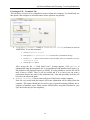
1.2. SysTune Startup
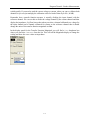
Run the Setup file (setup.exe) to launch the SysTune Startup application. Follow the instructions
on the screen to install SysTune, the NGINX webserver and the AFMG Licence Manager.
AFMG SysTune
This will create a folder (C:\Program Files\AFMG\EASERA SysTune) for the program
and place an AFMG SysTune icon on the Windows Desktop.
The installer will also automatically create two sample file subdirectories; the directory
\Signals\ contains a selection of excitation signals, the directory \IRs\ contains a set of
impulse responses.
AFMG Licence Manager
This will create a folder (C:\Program Files\AFMG\AFMG Licence Manager) for the
program and place an AFMG Licence Manager icon on the Windows Desktop.
NGINX Webserver
This will create a folder (C:\Program Files\AFMG\NGINX Webserver) for the
program. The webserver is a prerequisite for the SysTune Web Interface.
1.3. SysTune User Files
Finally, open the SysTune User Files zip file and run the included file. Select Typical to
install with the preferred settings. This will make the software licence available to all users of
this computer. Select Customize if you would like to change this preset to a different location.
The installer will then create a folder for the user files and allow you to use the AFMG Licence
Manager installed above to register a licence for the software.
1.4. Licencing the Software
Please follow the steps in the next section in order to register the program.
9
SysTune Installation and Licencing - Licencing Instructions
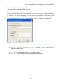
2. Licencing Instructions
Double-Click the AFMG Licence Manager icon on the Windows Desktop in order to license the
software.
2.1. Online Licencing
Online licencing allows you to easily download a SysTune licence via internet (being online with
your SysTune computer assumed). This means the software sends the computer's reference
information to our web application, which creates licence information on our server. This
information is then automatically downloaded and installed. So with a single button push on
Download Licence you can unlock SysTune.
By subscribing to the licence agreement you are entitled to install the program on a number of
computers equal to the number of licences (user keys) you have acquired. After performing that
number of installations, e.g. two, additional licences must be purchased if you intend to run the
software on more machines at the same time.
Please note: If you intend to uninstall SysTune from one or all of the original computers then
please upload the licence information from that computer by clicking on Upload Licence. This
will send the license to our server, allowing you to download this licence again and then unlock
SysTune on a different computer at your convenience. As a matter of fact, keeping licenses in
our server is more secure than in any computer.
2.2. Licencing by File
You should only use this option if you are not able to use the online licencing functions.
Reference File
The Reference File is a file generated by the AFMG Licence Manager program and placed
in the SysTune LicenceFiles folder. This file is different for each installation. If you have
more than one computer each will have its own Reference File. To order a licence you
must send the Reference File to AFMG ([email protected]) by E-Mail.
Licence File
The Licence File is a file generated by AFMG, which is linked to the Reference File.
The Licence File is supplied to you by E-Mail. Loading this file into the AFMG Licence
Manager with Install Licence unlocks the particular SysTune version purchased.
If you intend to uninstall SysTune from one or both of the original computers then remove the
licence information from that computer before by using the Termination. Terminate
Licence creates a Termination File which you must send to AFMG by E-Mail. This
will allow you to order a new licence for the terminated one and unlock SysTune on a different
computer or computers. There can be only as many operational programs at the same time as you
have licenses!
10
SysTune Installation and Licencing - Licencing Instructions
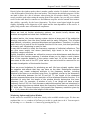
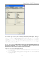
2.3. AFMG Licence Manager Program
This program allows the licencing of SysTune.



Proxy Settings: Opens the proxy server configuration window. It allows adjusting
proxy server settings for online licencing through a proxy server.
see also:
Proxy Server Configuration Window
About: Shows information about the currently installed AFMG Licence Manager.
Exit: Closes the AFMG Licence Manager window.
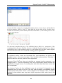
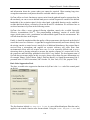
Licence Status
 Online Licencing: Shows the Online Licencing Tab in the right part of the
AFMG Licence Manager.
 Licencing by File: If it is not possible for you to be online with your computer a
SysTune licence can be ordered via email instead. To do that, generate a reference file
and send this file to AFMG ([email protected]). As a response you will receive a licence
file from AFMG which is needed to unlock SysTune.
This button enables three tabs in the right part of the AFMG Licence Manager labeled
Licence, Terminate, and Import/Export. See below for instructions on how to
use these tabs.
11
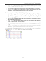
SysTune Installation and Licencing - Licencing Instructions





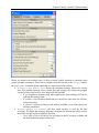
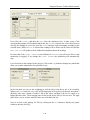
Software Product: This field shows the AFMG software product selected for
licencing.
Registered Company: This field shows the company name for which the installed
licence is registered.
Number of Licences: This field shows how many licences are available on this
computer.
Licenced Version: This field shows which software version is unlocked.
Refresh Licence Info: Reloads the licence information.
Online Licencing



Info: Checks the SysTune licence database on the AFMG web server and downloads
information about the user registration, the purchased version and the number of licences
still available.
Download Licence: Downloads one licence from the AFMG web server. The
number in the Number of Licences field will be increased by one.
Upload Licence: Terminates all available licences. The licences will be uploaded
to the AFMG web server and will be available for new downloads later. If you intend
hard disk manipulations or to buy a new computer you should use this procedure to
prevent a licence being lost. It just means a licence backup for a certain time. After this
procedure SysTune will reset to an unlicenced mode.
12
SysTune Installation and Licencing - Licencing Instructions
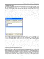
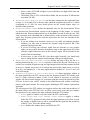
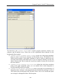
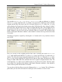
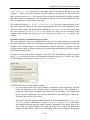
Licencing by File – Licence Tab
This tab allows a licence to be installed on this computer. You should only use this option if this
computer is not online and a licence download is not possible.


Create Reference File: Creates a Reference File (*.erf format) to send to
AFMG/SDA. To use the command:
1.
Click on Create Reference File.
2.
This opens a Save Reference File window after a confirmation message.
3.
Use the Save In portion of the window to select the folder where you would like to save the
Reference File.
4.
Click on the Save button.
After saving the file, a "Send Email now?" prompt appears. Click on Yes to
automatically send a licence order with the reference file as an attachment using an
installed email client (e.g. MS Outlook or MS Outlook Express) to AFMG. It is also
possible to save the file and to mail it later attached to a licence order to AFMG.
Install Licence: Click to load a licence file (*.elf format) and install a licence for
SysTune. To use this command: Click on Install Licence.
1.
This opens an Open Licence File window.
2.
Use the Look In portion of the window to find the folder containing the licence file.
3.
Click on the Licence File name.
4.
Click on the Open button.
If the reference signature in the Licence File matches this computer, the licence will
be installed. The licence information and parameters will be shown in the Licence Status
frame.
13
SysTune Installation and Licencing - Licencing Instructions
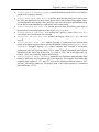
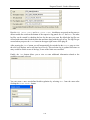
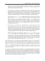
Licencing by File – Terminate Tab
This tab allows a licence to be uninstalled or removed from this computer. You should only use
this option if this computer is not online and a licence upload is not possible.


Terminate Licence: Creates a Termination File (*.etf format) to send to
AFMG/SDA. To use the command:
1.
Click on Terminate Licence.
2.
This opens a Save Termination File window after a confirmation message.
3.
Use the Save In portion of the window to select the folder where you would like to save the
Termination File.
4.
Click on the Save button.
After saving the file, a "Send Email now?" prompt appears. Click on Yes to
automatically send the termination file as an attachment using installed email client (e.g.
MS Outlook or MS Outlook Express) to AFMG. It is also possible to save the file and to
mail it later to AFMG. There it will be verified and if it is correct you can order a
replacement licence any time for the terminated one. After this procedure SysTune will
be reset to an unlicenced mode.
Remove Licence: Click to remove all traces of the licence on this computer.
Note: Be very careful with this button! All licence information will be deleted from the
computer. This option should only be used in case of general licencing problems due to
software or hardware errors. Please contact AFMG before using this command or your
SysTune licence may be lost completely.
14
SysTune Installation and Licencing - Licencing Instructions
Licencing by File – Import / Export Tab
This functionality is not supported by SysTune.
Proxy Server Configuration Window
If you are running SysTune in a secured intranet, access to the internet for online licencing may
be blocked by a firewall, depending on your network’s configuration. Configuring AFMG
Licence Manager to use the local proxy server on your network may resolve this issue. If you are
unsure of the appropriate proxy server settings, please consult your network administrator.
Use the following proxy server
 Server Name [:Port] : Proxy server name or IP address and port number for
internet access.
 Server requires Authentication: Check if the proxy server needs an
additional authentication.
 Account Data: User name and password to authenticate on the proxy server.
 OK: Accepts configuration settings and closes the window.
 Cancel: Discards configuration settings and closes the window.
15
Program Tutorial - Introduction
Program Tutorial
1. Introduction
Preface
This part of the SysTune Tutorial is a guide that explains step-by-step all of the important
functions of the software and their background in acoustic measurements. It is recommended that
you work through this guide at least once if you are a beginner with SysTune or with measuring
software in general. Advanced users can also gain new insights from the following exercises,
because the software represents a new approach to making live-sound measurements in several
respects.
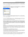
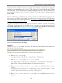
The next sections will assume a fresh installation and the software in its default configuration. If
you have already worked with the software before, make sure you reset all of the configuration
data first by selecting AFMG SYSTUNE (USE DEFAULT SETTINGS) from the Windows Start Menu
under AFMG  EASERA SYSTUNE . Otherwise some displays and calculation results may
look different from the ones presented here.
For simpler printing, our explanations use screen shots based on the standard system colors
scheme, rather than the default color scheme with bright colors on a black background. To use
the same colors as we do, go to the menu labeled CONFIGURE, the sub menu COLOR SCHEME and
then select the menu item SYSTEM COLORS.
At this time let us agree about a convention for references to the graphic user interface of the
software: We will describe items by the sequence of labels in the hierarchy of the controls in the
user interface. In the above case, the full reference would be CONFIGURE|COLOR SCHEME|SYSTEM
COLORS. In simpler cases we may just refer, for example, to the OK and CANCEL button of a
window in the same manner.
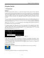
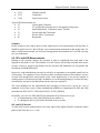
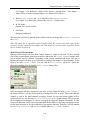
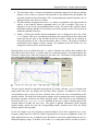
Starting the Software
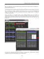
To start the software click (or double-click) on the AFMG SysTune icon on your desktop.
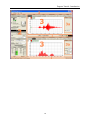
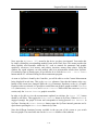
Upon start-up SysTune will show you a screen like the following:
16
Program Tutorial - Introduction
Note that the right figure already shows the program window in system colors. We switched to
this alternative, printer-friendly color scheme using the menu command CONFIGURE|COLOR
SCHEME|SYSTEM COLORS.
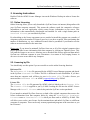
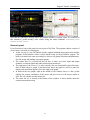
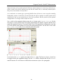
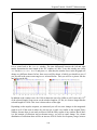
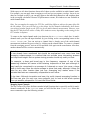
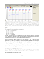
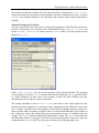
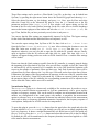
Screen Layout
Let us first have a look at the general screen layout of SysTune. The program window consists of
several areas, each with its own purpose:
 At the very top (1) you will find the window caption including the program name and the
program version number which is often helpful when you need software support. The
menu is located in the same area and gives access to all general functions and parameters,
like file saving and loading or program options.
 The control area (2) is located on the left; here is where you select input and output
channels, excitation signals and other measurement parameters.
 The right part of the screen (3) is split vertically into two functionally equivalent areas.
Each of them shows a graph, a selection menu above the graph as well as a panel for
display and calculation options (3a) to the right of the graph.
 In between the two graphs, right in the middle of the window, there is a bar (4) that
displays the current coordinates of the mouse and gives access to the mouse modes as
well. We will call this area the mouse bar.
 The status bar (5) is located at the bottom of the window. It shows details about the
current measurement setup.
17
Program Tutorial - Introduction
18
Program Tutorial - Measurements with a Single Input Channel
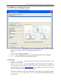
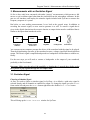
2. Measurements with a Single Input Channel
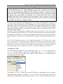
One of the most basic measurements one can do with a PC and a soundcard is monitoring an
input channel. This is what we want to do first; we will look at the signal at the input of the
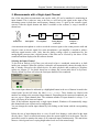
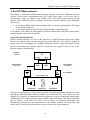
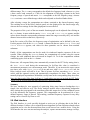
measuring system in both time and frequency domain views. To pick up the acoustic signal,
convert it into the digital domain and make it available to the software, a setup is needed as
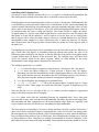
shown here:
Sound Wave
Microphone
Pre-Amplifier
ADC
PC
Analog-Digital
Converter
Computer +
Software
A measurement microphone is used to record the acoustic signal of the sound pressure field and
convert it into an electric signal. For most microphones a pre-amplifier is needed to achieve
sufficient signal-to-noise ratio. After that the analog voltage signal is transformed by the
analog/digital converter into a digital stream of bits that can be received by the driver of the
soundcard and then displayed in the software domain.
Selecting the Input Channel
To do such an analysis in SysTune you only need to have a soundcard connected to or built
inside your computer. When the software is started it will automatically choose the audio device
that is already selected as the default device for audio playback and recording in Windows
(please see chapter 5.3 for details about how to change the current audio driver in SysTune).
Also by default, SysTune will select the first input channel of the soundcard.
The current input channel is indicated by a highlighted button in the row of buttons located in the
control panel on the left below the label SIGNAL CHANNEL. These buttons are labeled with
numbers according to the associated input channels. Depending on the connected soundcard you
may see up to 8 input channels here. The minimum number of input channels is always 2, so
there will always be at least two buttons.
Note: If the hardware supports only a single input channel, Windows will automatically image
this channel and create a quasi-stereo configuration.
You can change the current input channel by left-clicking on the button with the corresponding
number.
Below the row of input buttons there is a row of small level displays, each related to the input
directly above. These so-called mini-meters show the current signal level at the input. They are
particularly useful to monitor the status of all connected inputs simultaneously. The mini-meter
shows a vertical green bar of varying height when levels are in the normal range.
19
Program Tutorial - Measurements with a Single Input Channel
However, when the signal at the port of the A/D converter is greater than the maximum that is
possible for the electronics, the input signal is clipped upon conversion. The mini-meters indicate
proximity to clip level by yellow color, for –6 to –1 dB below clip level, and by red color, for
signals of –1 dB below clipping and higher. To ensure the data validity of your measuring
system, make sure that you do not exceed clip level at any time. It is good practice to adjust the
gain control in such a way that the peaks of the signal are maximally in the yellow range.
Hint: Because clipping can happen for only very short periods of time, such as during signal
peaks, you may not always be able to catch the red bar lighting up with your eyes. For this
reason, the frames of the mini-meters remember the last clip state in the order of green-yellowred until reset with a mouse click directly on the mini-meter.
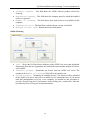
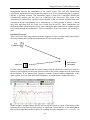
2.1. Time Signal
Now let us look at the input signal as it arrives in the software domain. In the default
configuration, the software starts with the TIME SIGNAL button selected for the top graph. Along
with the graphs SPECTRUM and SPECTROGRAM in the same group, this display can be used
immediately for any kind of INPUT signal without adjustment of additional parameters.
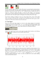
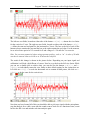
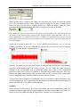
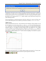
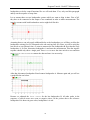
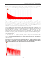
If there is no signal except for noise at the input, the graph will look similar to the following
picture and it will be continuously moving from the right to the left.
If the graph does not change with time, make sure you have started the real-time analysis, it is on
by default for the very first program start. To do that look at the control panel to the left, right
below the INPUT section. If the first large button is labeled START ANALYSIS, the real-time
functions of SysTune are currently suspended. Left-click on the button to restart the analysis. If
the button is already labeled STOP ANALYSIS and it is highlighted, the TIME SIGNAL graph
should be updating continuously. If this is not the case, please refer to the trouble shooting
section at the end of the tutorial.
20
Program Tutorial - Measurements with a Single Input Channel
Let us return to the TIME SIGNAL graph. The horizontal axis shows the time passed by,
maximally for the period of the current FFT block size; we will come back to that a little bit
later. The vertical axis shows the signal amplitude in digital units, also called full-scale (FS).
Because generally SysTune does not know which hardware is being used, it cannot display realworld numbers like Pascals (Pa) or Volts (V) directly. But the software can be calibrated very
easily. Calibration here means giving the software a relationship between digital values, which is
the only thing the software really knows about, and physical values, as they can be measured in
the real-world.
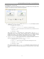
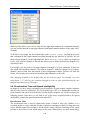
Calibrating an Input Channel
Now we would like to calibrate the first input channel. If you have switched to a different
channel in the meantime, click on the button labeled 1 to activate the first channel again. Right
below the mini-meters, the software shows an area related to the properties of the input that is
currently selected. The fields GAIN and DELAY, as well as the PEAK and AUTO buttons, correspond
to parameters that we will investigate in a little while; we will first focus on the calibration. It
can be started by a left-click on the CALIBRATE button below the PEAK button. Note that the
current calibration status is always shown to the left of the CALIBRATE button. If the input has not
yet been calibrated the label will show DIGITAL FS.
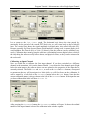
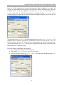
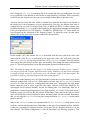
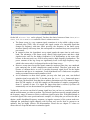
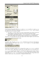
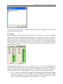
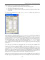
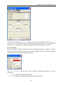
After pressing the CALIBRATE button the CALIBRATION window will open. It shows the ordinal
number of the input channel selected for calibration in the window caption.
21
Program Tutorial - Measurements with a Single Input Channel
Since we will be performing an acoustic measurement with a microphone, we need to tell
SysTune the relationship between pressure units, Pascals or dBSPL, and digital units, full-scale
or dBFS. This is exactly what happens on the first tab USE PRESSURE, the second tab USE
VOLTAGE can be used for electrical measurements. A third tab labeled USE CURRENT is only
available in the Pro version and can be used to generate impedance displays. How to do this will
be discussed in chapter 5.12.
The upper part of the CALIBRATION window displays the state of the CURRENT CALIBRATION. The
sound pressure level that is equivalent to a defined full scale level is shown in the dBSPL text
field. Later on, if you know the calibration for an input channel you can enter it directly here.
The check box labeled RMS (SINE) allows you to toggle between the display of the peak or the
RMS numbers for a sinusoidal signal.
For a full acoustic calibration do the following:
 put a microphone calibrator on the microphone,
 click on the START CALIBRATION MEASUREMENT button,
 wait until the value in the RMS LEVEL [dBFS] text field settles and then press the STOP
CALIBRATION MEASUREMENT button,
22
Program Tutorial - Measurements with a Single Input Channel

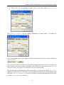
finally enter the corresponding pressure value in the field labeled RMS PRESSURE
[dBSPL], such as 114, and click on APPLY.
The CURRENT CALIBRATION will be updated immediately as shown below. To confirm the
calibration and close the window press OK.
Your measurement setup is now calibrated and the control panel will show the new calibration
state PRESSURE.
Hint: If you do not have a calibrator at hand while going through this tutorial, try to whistle into
the microphone and enter a value of 80 dBSPL. This will likely be right within an error of +/-20
dB and will allow you to follow the subsequent steps for calibrated data.
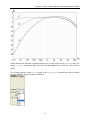
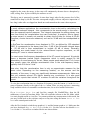
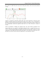
Having calibrated our measurement system successfully, we can now switch the TIME SIGNAL
display to a physical unit. To do that go to the right panel and change the current setting for the
unit from DIGITAL FS to PRESSURE. In case of a voltage or current calibration this list will allow
selecting VOLTAGE or CURRENT instead.
23
Program Tutorial - Measurements with a Single Input Channel
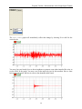
The TIME SIGNAL graph will immediately reflect that change by showing Pa or mPa for the
vertical scale.
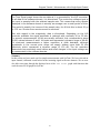
You may clap your hands close to the microphone or generate some other impulse-like noise to
see the effect in the graph. You may even let the input clip just for this moment. Have a short
look at the mini-meter and how it reacts to the changing input signal.
24
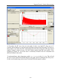
Program Tutorial - Measurements with a Single Input Channel
In the TIME SIGNAL graph you will notice that the vertical axis is scaled automatically to a larger
section to show all of the data that arrives. However, it does not automatically collapse to the
original range after the spike has left the displayed period of time. That is because the program
expects more signals of that order of magnitude and therefore remembers the maximum view
limits. To reset the view just double-click on the graph.
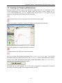
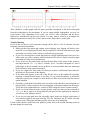
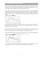
Adjusting the View Limits
Now it is time to look more closely at the scaling of the diagram. By default, the current mouse
mode is the ZOOM mode, as indicated in the mouse bar.
In this mode you can use the left mouse button to zoom into the graph with respect to the
horizontal axis. To do that, left-click on the start value for the new view limits and keep the
mouse button pressed while dragging the mouse pointer to the stop value. While dragging, the
program will indicate the current start and stop values by vertical lines or zoom markers. Finally,
release the mouse button to confirm the new view window. Also in ZOOM mouse mode, you can
use the right mouse button to select the view limits in a similar way for the vertical axis.
Hint: The zoom markers snap to the lines of the graph. To freely select the zoom area, keep the
Alt key pressed while dragging the mouse.
Let us try out the DRAG mouse mode, too. Select this mouse mode by first clicking on the button
labeled DRAG in the Mouse bar, then left-click on the graph and keep the left mouse button
pressed. When you now move the mouse you can shift the current view port freely. The PEEK
mouse mode is the third mouse mode available for all graphs, but we will come back to it at a
later point of time, when there is more meaningful data to peek at.
At any time you may return to the full view limits by double-clicking in the graph area or by a
left click on the auto-scale button in the upper left corner of the graph.
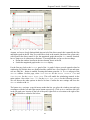
In addition to changing the view limits with the mouse, you can also enter them directly as
numerical values. To do this we need to open the view limits section with a left click on the
triangle button in the lower left corner of the graph.
This command slightly rescales the graph vertically to create some space for a new panel; the
view limits section, shown in the next picture.
25
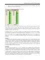
Program Tutorial - Measurements with a Single Input Channel
The left two text fields, located on either side of the button <-Y[PA]->, denote the view limits
for the vertical or Y-axis. The right two text fields, located on either side of the button <-X[S]>, define the start and end point for the horizontal or X-axis. The box to the left of each of the
buttons always contains the start and the box to the right contains the end value. For the moment,
let us select a time period of 1.2 seconds for X and a range of +/-30 mPa for Y to exercise.
Hint: You can enter numerical values using exponent prefixes, such as “m”. A value of 30 mPa
can thus be entered either as 0.030 or as 30 m into the text field.
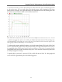
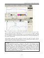
The result of this change is shown in the picture below. Depending on your input signal and
calibration it will look a bit different, of course. Now let us go back to the full view limits. While
you can use a double-click to achieve that, you can also use the buttons <-X[S]-> and <Y[PA]-> to individually return the view limits to their default setting for the current data set.
Left click on <-X[S]-> to scale the horizontal axis to contain all data points, left click on <Y[PA]-> to do the same for the vertical axis.
Now that you have learned all of this you should be able to pick up a signal with the microphone,
stop the analysis for a while, zoom into the sound event to look at it as a function of time, zoom
back to the full view and start the real-time analysis again.
26
Program Tutorial - Measurements with a Single Input Channel
Tech-Note:
The Time Signal graph shows the raw data as it is generated by the A/D converter.
As all data in the software domain, it is discretized. The continuous voltage signal at
the input is sampled with the selected sample rate. This means that every sample
displayed in the software domain is actually an average over a small period of time.
This period is exactly the inverse of the sample rate, for 48 kHz this is about 20 μs
or 0.02 ms. Shorter time events cannot be resolved.
Also with regard to the magnitude, data is discretized. Depending on the A/D
converter available the signal amplitude is rastered with nominally 16 to 32 bits.
For acoustic measurements 16 bits are usually sufficient, this corresponds to about
32,000 values between 0 and 1 full-scale and represents a dynamic range of 96 dB.
For electronic measurements a higher resolution is often desirable, although
soundcards in the normal price range will supply seldom more than 20 bits
effectively which represents a dynamic range of 120 dB. The bit resolution
determines how accurately small values and small changes in the input voltage can
be represented in the software domain.
Summary
In this section we have made our first simple measurements with SysTune. We have selected an
input channel, calibrated it and looked at the incoming signal in the time domain. We are now
also able to navigate through the displayed area of the TIME SIGNAL graph with functions that
work the same for all graphs in SysTune.
27
Program Tutorial - Measurements with a Single Input Channel
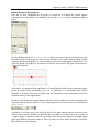
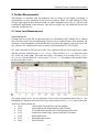
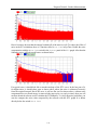
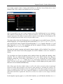
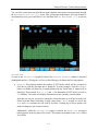
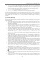
2.2. Input Spectrum
We just looked at the input data in the time domain; now let us take a look at the same data in the
frequency domain. In the default configuration, SysTune starts with SPECTRUM selected for the
bottom graph. This view shows the frequency data that corresponds to the time data in the upper
graph TIME SIGNAL.
By default, the diagram is shown as a bar display in 1/12th octave resolution and with no
weighting applied. Depending on the dynamics of the input signal you will also see a second
curve, namely the peak hold curve. It shows the short time history of the spectrum curve.
Note that the default view for the vertical axis includes a range of -90 to 0 dB. If your soundcard
has a very low noise floor the graph may show only a small part of the curve or nothing at all. To
see more, you may have to change the view limits to a range of -120 to 0 dB, for example, or
increase the level of the input signal alternatively.
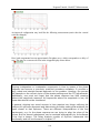
Peak hold
In the right panel on the DISPLAY tab you can select settings different from the above and we will
go through them now briefly. The first selection that can be made is the WEIGHTING applied to the
28
Program Tutorial - Measurements with a Single Input Channel
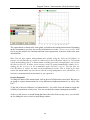
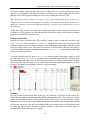
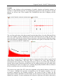
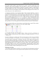
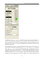
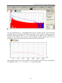
frequency data. The three weightings A, B, C superimpose different correction curves to take into
account the characteristics of human hearing.
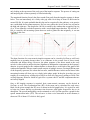
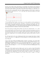
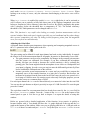
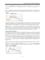
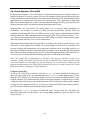
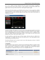
The human ear is less sensitive to signals at low and high frequencies compared to the mid-range
around 500 Hz to 4 kHz. Therefore, sound level measurements do not correspond directly to the
perceived loudness of a signal. Weighting curves have then been developed so that broadband
level values correlate more closely to the human hearing. A weighted display of the input
spectrum accounts for this effect as it shows the levels as they would be perceived according to
the A, B or C weighting standards (ANSI S1.4 (A, B, C) or IEC 61672-1 (A, C, Z)). In fact, the
different weighting functions have their background in different types of signals, like pure tones
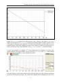
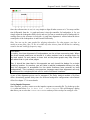
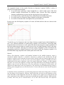
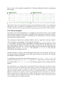
or noise, which are – again – perceived differently by the human hearing system. The following
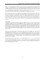
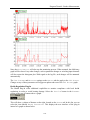
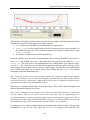
picture shows the A, B and C weighting filters as a function of frequency.
29
Program Tutorial - Measurements with a Single Input Channel
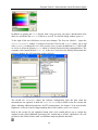
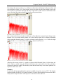
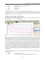
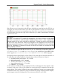
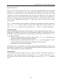
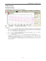
Switch between the different weighting functions to see their effect on the SPECTRUM data. The
setting Z (NONE) will always take you back to the unweighted (also called zero, flat or linear)
graph.
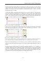
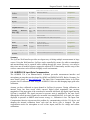
The second parameter in the DISPLAY panel is the RESOLUTION. It controls how wide the bands
are over which the frequency data is combined.
30
Program Tutorial - Measurements with a Single Input Channel
The result of applying an FFT to the time data is frequency data with linear spacing, which
means equal spacing between adjacent frequency data points. To display this data in fractional
octave bands like 1/1 or 1/12 all of the data points lying in one band are summed to a single
value to obtain the level for that frequency band. The FULL resolution is the only resolution
where the data is displayed raw, although it is seldom used.
Tech-Note:
Pink noise has the characteristic property that it is a flat curve when shown in
summed fractional octave bands. This type of view corresponds to the power
contents of the signal. The same holds true for other pink signals, which are signals
with a 3 dB drop of power density per octave band, like a log-sweep. In contrast,
signals with constant power density over frequency, like White noise, show levels
increasing with frequency in such a summation graph.
When using the Full resolution graph the behavior will change, because now the
program displays power densities instead of powers, that is, summed power
densities. In this kind of graph White noise is represented by a flat function of
frequency and Pink noise as a curve decreasing in level by 3 dB per octave.
31
Program Tutorial - Measurements with a Single Input Channel
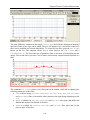
Finally, the SPECTRUM display can be shown in two ways, either as a bar graph or as a curve
graph. Use the check box BAR DISPLAY to toggle between them. While it is more common to use
a bar graph for fractional octave diagrams, it is often more difficult to use this kind of view for
analysis purposes. Especially looking at overlaid curves which we will discuss in detail below is
much easier for lines only. Note that there is no BAR DISPLAY for the FULL resolution setting.
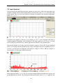
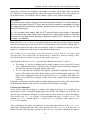
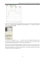
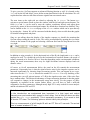
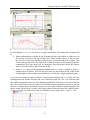
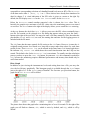
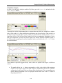
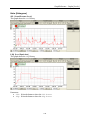
For now, let us choose no weighting, 1/3rd octave bands and a curve display. As we have also
already calibrated the input channel, we may also select PRESSURE as the UNIT. After making
these selections you should see a screen like the one below.
Also this display is still based on the raw data from the input, just with different calculation
parameters for the post processing. The original time domain data is continuously retrieved by
32
Program Tutorial - Measurements with a Single Input Channel
the program, transformed into the frequency domain and displayed as a spectrum, which is level
as a function of frequency.
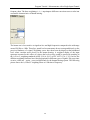
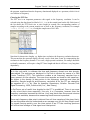
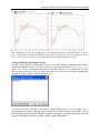
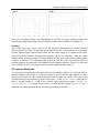
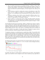
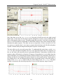
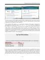
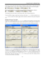
Choosing the FFT Size
The FFT size is an important parameter with regard to the frequency resolution. It can be
selected using the drop down list labeled FFT SIZE in the control panel on the left. Each item of
the list shows the FFT block size or time length in seconds, the corresponding number of
samples according to the current sample rate as well as the frequency resolution, for example
1.49 S; 65536; 0.67 HZ, if using the sample rate of 44.1 kHz.
Note that for shorter time lengths, e.g. higher time resolution, the frequency resolution decreases.
This means that the spectrum display can only resolve short time events by compromising the
resolution in the frequency domain. Vice versa, a high spectral resolution, for example desirable
to identify resonances, will require a long FFT time length and thus it will have a very long time
dependency.
Tech-Note:
As in the real world, in software the time and frequency domain are also strongly
interrelated. The spectrum as displayed in SysTune is derived by means of a Fast
Fourier Transform (FFT). This transform creates a set frequency samples from a
given amount of time samples. The more time samples are used for the transform,
the higher is the density of data points in the frequency spectrum and thus the
resolution. Sample length Δt and frequency resolution Δf for the FFT are related by
the equation Δf = 1 / Δt. (See for example: Oppenheim, Schafer: Discrete-Time
Signal Processing, 1999, Prentice-Hall, Inc., New Jersey)
In SysTune a set of useful time lengths for the FFT is predefined. There is no sense
in very short block sizes especially, like only 4 or 8 samples, because then the
frequency resolution becomes far too low. Very long block sizes like several minutes
are also not available, because the measuring times become impractical.
Since each frequency data point is derived from all time samples of the given block,
the resulting data must be understood as an average over the full time length used.
For signals varying quickly over the time period of an FFT the resulting spectrum
will be the time-average of that signal over that period.
33
Program Tutorial - Measurements with a Single Input Channel
Another important point with respect to the FFT is that generally some windowing
must be applied to the FFT block. Because a cyclic FFT is used for the transform
from the time domain, any abrupt changes between the start and the end of the
block will cause disturbing artifacts in the frequency domain. A flat-top window
applied to the FFT block helps to smoothen this transition and is particularly needed
for signals that are smooth and periodic, like a sine wave, but with a period
different from the FFT block length. (See for example: Fredric J. Harris: On the Use
of Windows for Harmonic Analysis with the Discrete Fourier Transform, Proceedings
of the IEEE, Vol. 66, No. 1, January 1978)
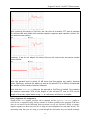
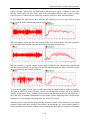
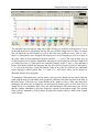
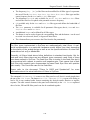
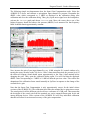
Let us have a look at the effect of changing the FFT size. Select a time length of 3 seconds or so
and create a sharp, loud impulse at the microphone. You will see that the spectrum increases
immediately, stays elevated for the time of the FFT block length and then drops to its original
state. Now switch to a short FFT block length, such as about 0.2 seconds. Again, create an
impulse and watch the spectrum rise and decay. In practice, there will seldom be a need for FFT
sizes beyond these lengths.
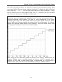
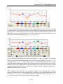
Also, have a look at the frequency resolution at this time. For an FFT size of 0.2 s the spacing
between frequency points is about 5 Hz. You will recognize that at the low end of the spectrum,
the graph looks stepped and very rough. This roughness in frequency is due to the fine resolution
in time. However, in practice you will seldom need frequency resolutions much higher than 5
Hz.
Hint: The FFT calculation requires a lot of computer performance. Your PC may not be suited
for very short FFT sizes. If that is the case, audio samples of the input or output audio streams
might be lost. Whenever using small FFT sizes make sure to check the status bar at the bottom of
the window. It will show a warning when samples are being dropped. On standard computers
this typically happens in the range of a size of 512 or 1024 for a sampling rate of 48 kHz.
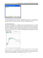
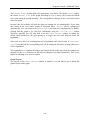
Averaging over Time
The second important parameter for the calculation of the INPUT SPECTRUM is the number of
AVERAGES. You will find the drop down list right below the FFT SIZE selection in the
PARAMETERS section. This list shows the number of FFT blocks to be averaged and the
corresponding overall time length.
The number of AVERAGES defines how many FFT blocks are transformed into the frequency
domain and then averaged to yield the SPECTRUM. The longer you average the data, the less
significant will singular time events affect the overall SPECTRUM. Also, the signal-to-noise ratio is
34
Program Tutorial - Measurements with a Single Input Channel
increased by 3 dB for every doubling of the number of averages. On the other hand, just like the
FFT block size, a long averaging time reduces the temporal resolution. When you average over
20 seconds of time, you will not be able to identify a peak of a few milliseconds length.
Tech-Note:
The overall time is what counts for the acquired spectrum data. The main reason to
split the time length into an FFT block size and into a number of averages is to keep
the performance requirements practical, because they can become too high for very
large FFT block sizes.
So, for the same time length, half the FFT size and twice the number of averages
will yield about the same result. Note that this will change the frequency resolution
and some of the data as well because a different number of FFT windows – one per
average - are applied.
Below the label AVERAGES there is a small horizontal meter that shows the time that has elapsed
since the measurement was last started and it is shown relative to the overall averaging time. It
indicates how much of the data in the current display actually is valid data. At any time you may
hit the RESET button next to the meter to restart the measuring process.
Hint: Assume you are performing a spectrum analysis in a venue and you are using a long
averaging time. Now, unexpectedly, the measurement is disturbed by someone shutting a door,
then just push the Reset button to restart the data gathering process.
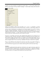
At the bottom of the list of AVERAGES you will find additional selections, EXP and INF:
 The setting INF lets the averaging process simply continue forever instead of covering
only a limited period of time. This option may be helpful when the maximum number of
Averages does not provide enough signal-to-noise ratio.
 The EXP item also runs infinitely but it applies exponential weighting to the averaging
process. This makes time blocks further in the past less important than recent ones. The
slope of the weighting function can be selected in the OPTIONS window. This function is
useful if you would like to monitor average levels with a smooth roll-off of high peaks
over time.
Remember in this respect that the regular averaging settings provide a hard cut-off, which makes
peaks disappear abruptly when they leave the time period selected for averaging.
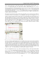
Checking the Calibration
So far we have only been looking at a random noise signal at the input. It is certainly just as
interesting to see how a sinusoidal signal appears in SysTune. The simplest way to do that is to
take the same microphone calibrator we used a little bit earlier and put it on the microphone.
Also, switch to an FFT SIZE of about 1.5 second length and select 1 for the AVERAGES. The
frequency RESOLUTION should still be 1/3 and no WEIGHTING should be used, return to a BAR
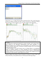
DISPLAY for a moment.
After switching on the signal, you should see a fairly large horizontal bar in the TIME SIGNAL
graph and a distinguished peak above some noise floor in the SPECTRUM. You may have to
double-click into each drawing to get back to the full view. If you have calibrated the input as
35
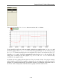
Program Tutorial - Measurements with a Single Input Channel
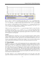
described before, you can also switch the current UNIT to PRESSURE for both top and bottom
graphs. They will then look approximately like the following.
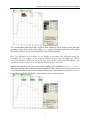
If the input was calibrated correctly, then the Spectrum should now show a peak at the
calibration frequency (here 1000 Hz). For that frequency band, the sound pressure level of the
bar should be the same as the level you calibrated to (here 114 dBSPL), maybe it will be off by a
tenth of a dB. You can verify this by zooming into the area of interest, but there is an easier way
as well. You may have already noticed that whenever you move the mouse over the graph a
green cross is following the mouse, tracking precisely the current curve. The values that
correspond to the location of the tracking cross on the horizontal and vertical axis can be viewed
on the mouse bar; it is centered between the top and the bottom graph. Note that the read-outs are
always related to the graph where the mouse is hovering. Carefully move your mouse close to
the location of the peak. Let the tracking cross settle on the top of the peak and look at the mouse
bar. It should now be showing the frequency and level of the peak.
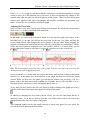
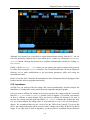
For further analysis, stop the measurement for a while (STOP ANALYSIS on the left side) as well
as the calibrator and zoom into the upper graph, the TIME SIGNAL. If you zoom in (drag using the
left mouse button), you will immediately recognize that the horizontal bar is actually a
graphically compressed sine wave signal. Again, use the mouse tracking cursor, find the
maximum and read it off the mouse bar.
36
Program Tutorial - Measurements with a Single Input Channel
In our case we find approximately 14.2 Pa which equals 117 dBSPL. At first glance, this seems
wrong as we measured a 114 dBSPL before in the frequency domain. However, here we need to
distinguish between peak values, like the maximum shown in the TIME SIGNAL, and RMS (rootmean-square) average values, like shown in the SPECTRUM. For a sinusoidal wave the peak value
is 3 dB higher than the RMS value and that is exactly what we found.
Hint: Repeat this relationship in your mind for a moment, because we will encounter this more
often while working with the software. It is important to understand that some parts of the
program show peak values, while others will use RMS values. It depends on the purpose which
type of value is needed or used. Regarding measuring platforms it can happen that errors sneak
into reports or analyses when it is not clearly distinguished between peak and RMS. If you talk
about the level of a signal, make sure you always mention what kind of level you refer to.
Summary
We have introduced the input spectrum as another way to look at the data recorded by the
microphone. We have talked about various display parameters like the weighting curve and the
resolution. We have also introduced the measuring parameters FFT size and number of averages.
In this respect we discussed about the trade-off between time resolution and frequency
resolution, this relationship will become even clearer in the next section when we look at the
spectrogram. Finally, we looked at the signal of an external sine wave generator in both time and
frequency and verified the calibration.
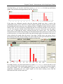
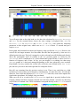
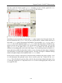
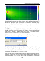
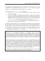
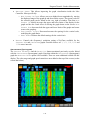
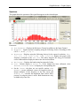
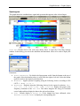
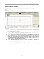
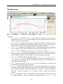
2.3. Spectrogram
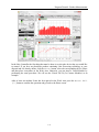
The SPECTROGRAM is the third type of graph available for input data. Switch the upper graph from
TIME SIGNAL to SPECTROGRAM to see it. Rather than a line or bar graph the display now shows a
color map that is continuously moving from the bottom to the top. But only at first glance it
looks much different from the Spectrum graph that we investigated a little earlier.
37
Program Tutorial - Measurements with a Single Input Channel
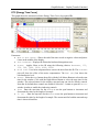
You will notice that on the right hand we also have the selections for WEIGHTING, RESOLUTION
and UNIT. For the moment please choose the same settings as displayed here: NONE for
WEIGHTING, 1/12 for RESOLUTION and DIGITAL FS for UNIT. Also return the measuring
parameters to their original state, which were an FFT SIZE of about 1.5 seconds and just a
single AVERAGE.
In the graph, the horizontal axis shows the frequency range just like the SPECTRUM. However, the
vertical axis no longer measures level but rather the time that has passed by, from now to a
defined point in the past. The level is mapped to a color scale and you will find that scale directly
above the spectrogram itself. In contrast to the two previous graphs we looked at, the
SPECTROGRAM can be considered to be a three-dimensional graph because it shows level as a
function of frequency and of time. In fact, you can imagine it as nothing else than many
SPECTRUM graphs in a chain and arranged depending on the time when they were recorded.
Equivalently, you may consider the vertical axis as the time axis defined in the TIME SIGNAL
plot, but now you can see the whole spectrum for each point of time.
But still, our reasoning from the previous section is true. There is no such thing as a high
resolution of events in time and in frequency simultaneously. To make this clear, we will run a
short test. First switch the displayed RESOLUTION to 1/96. After that, create some impulse-like
signal at the microphone, for example, clap your hands.
What you will see as a result in the SPECTROGRAM is a signal that is precisely defined in the
frequency domain and that is strongly smeared out in the time domain - note the very thin long
vertical lines of constant color. These resolutions correspond directly to the FFT SIZE selected
before.
38
Program Tutorial - Measurements with a Single Input Channel
Now, change the FFT SIZE to something like 0.05 seconds and clap your hands again. You will
see a signal that is well defined in time but has a rough frequency resolution. This is especially
visible for the low frequencies where you can see long horizontal lines of the same color.
You may not see exactly the same results as printed here; naturally the actual levels depend on
the sensitivity of the microphone, on your soundcard etc. However, the default color scale is
configured to be very wide, covering a range from –90 dBFS to 0 dBFS. To obtain a better color
resolution check the SPECTRUM graph at the bottom for the approximate minimum and maximum
levels you would like to see. This might be –120 dBFS to –60 dBFS for 1/12th octave bands, the
levels depend on the resolution of the frequency bands. To adjust the colors for that range,
double-click on the color scale to open a window like the one below:
In this window, the value entered for MIN is associated with the lower end of the color scale
(blue) and the value for MAX is associated for the upper end of the color scale (red). Note that
under COLOR MAPPING you can also switch from RGB to GRAYSCALE if needed. This will map the
lower end of the scale to black and the upper end to white. Now change the limits as desired and
press OK. This will immediately rescale the spectrogram plot and use the new colors.
Hint: The ability to change the color range is very useful in practice. It allows you to “zoom in”
to a range of levels and recognize differences more clearly. Similarly, you may select wide limits
to suppress details and get a fast overview over the dynamic range of the input signal. The
grayscale is useful e.g. for generating black & white result graphics.
With respect to the frequency axis, all of the functions to select the view port can be used: mouse
functions, manual entry, full view etc. With regard to the time axis, the SPECTROGRAM is limited
in so far, as it does not allow for a starting time other than zero. Consequently the right mouse
button cannot be used to select a specific time range. Only the overall time length for the
spectrogram can be entered manually, but not its starting point. It is noteworthy, that due to
performance reasons the spectrogram data is not kept explicitly. As a result, if you zoom in into a
frequency region you will lose the data outside of that range. Upon return to the full view blank
areas will be shown for those frequencies where the history data was not recorded. Remember,
that you can stop the SPECTROGRAM at any time using the button STOP ANALYSIS in the control
panel on the left.
Only for the SPECTROGRAM there is a command called SWITCH ORIENTATION which allows you to
swap the vertical and horizontal axes. Depending on the type of investigation and the available
screen area you might be interested in more screen space for the frequency domain or for the
time domain. The default configuration is with the horizontal axis showing frequency. This
39
Program Tutorial - Measurements with a Single Input Channel
makes it easier to align the view to the SPECTRUM when that graph is shown as a second display
above or below the SPECTROGRAM.
As we outlined earlier, the main purpose of the SPECTROGRAM is to have a history of the input
spectrum over time. On the one hand, this is very useful to obtain an impression of the spectral
distribution of a sound event after it has already disappeared in the SPECTRUM graph. On the other
hand, the SPECTROGRAM can be employed in the frequency domain to search and investigate
resonances and find feedback situations.
Synchronizing Views
You may have noticed that the SPECTROGRAM graph and the SPECTRUM graph now show another
icon in the upper left corner, right below the auto-scale icon:
This so-called SYNC icon allows you to synchronize the horizontal view limits of the two current
graphs if they have the same axis, like here for SPECTROGRAM and SPECTRUM. The function is
available for both the time and frequency domain. Note that synchronization is defined as a state
function, that means that two graphs can either be synchronized or not. If synchronization is on,
both SYNC buttons are highlighted:
To try this out, use the mouse ZOOM to zoom into the frequency axis of the SPECTROGRAM graph.
Then press the SYNC button. As a result the SPECTRUM view will be switched to the same view
limits for the frequency axis. From now on, the software will keep the two views synchronous
with respect to the view limits. Whatever you do, they will be changing simultaneously until you
deselect either SYNC button. For example, use the auto-scale icon to return to the full view and
then zoom into the SPECTRUM graph. You will find that the SPECTROGRAM follows immediately.
Storing and Recalling Views
Let us use this opportunity to talk a bit more about manipulating the views of the upper and
lower graph. For example, right now we are looking at the SPECTRUM in the top graph and at the
SPECTROGRAM in the bottom graph. Assume you have adjusted the view in a way that is
particularly useful, for example, in looking for feedback in the mid-frequency range. The two
graphs could be synchronized as explained a bit earlier and they may be showing a bandwidth
from 250 Hz to 4 kHz.
There are a couple of different ways to save these view settings in order to recall them at a later
point of time. On the one hand, you can select SAVE VIEW FILE from the FILE menu. This
command will open a dialog window that allows you to save a view settings file (.stview) to your
hard disk. Using the OPEN VIEW FILE command from the FILE menu you can load this setting at
any later point of time. To try that out, save the current view and then change the view limits of
the frequency axis. After loading the view file back in, you will find that the original view limits
are restored. Loading the file will also restore the selected graphs for the upper and lower panels.
For example, the SPECTRUM view will be recreated if you had switched the upper graph from
SPECTRUM to TIME SIGNAL in the meantime.
40
Program Tutorial Another way to store and load view settings is by means of the VIEW menu. Notice that the menu
shows a set of 10 items at the top, labeled 1 through 10. Each of these memory slots can store a
particular view setting.
Saving a view setting to a slot is very easy. Select STORE CURRENT VIEW from the VIEW menu
and then choose the desired slot from the submenu below. After that, a small dialog window will
ask you to enter a label for the view setting just saved. In this example, let us use slot 5 and enter
the name “Spectrum Mid-Range”. Note that you can use the menu command RENAME VIEW to
assign a new label to any stored view setting. You can recall any saved view by just selecting the
desired menu item from the VIEW menu. Note that, initially, the first four items of the VIEW menu
already contain some simple presets that can be replaced as needed.
In practice, you will find yourself quite often switching among different views and using a set of
preferred view limits. The above procedures will help you to maintain some presets. But for even
more efficient working, SysTune provides a set of short cuts for storing and recalling views as
well. Press Ctrl+Shift+[N] to store a view in the Nth slot, where N is a number between 0 and 9
and 0 is assigned to the 10th slot. Use the key combination Ctrl+[N] to restore the view quickly.
Hint: It is most efficient to use only the first 9 slots for views that you use often for analysis or
creating reports. Use the 10th slot (short cut with 0) for storing views temporarily, e.g. when you
have to switch between graphs for just a moment and then go back to the exact same setting.
Summary
This section explained the third graph that is dedicated to the signal at the input, namely the
Spectrogram. Being a 3D graph it uses a color map to represent levels as a function of frequency
and time. We have seen how strongly interrelated time and frequency resolution are. We have
also discussed how view settings can be synchronized, stored and recalled.
41
Program Tutorial - Measurements with an Excitation Signal
3. Measurements with an Excitation Signal
So far we have only been concerned with rather “passive” measurements, which means we did
not use a real excitation signal other than the sinusoidal from the microphone calibrator. In this
part we will introduce and employ the stimulus signals included with SysTune to measure the
frequency response of a system.
But before we start making measurements, let us look at the general setup. In addition to
recording the acoustic signal, we now want to generate it as well. To convert a signal that is
given in the digital domain into the acoustic domain, an output chain must be established that is
similar to the input chain introduced earlier.
PC
DAC
Computer +
Software
Digital-Analog
Converter
Amplifier
Loudspeaker
Sound Wave
The software on the computer provides the driver of the soundcard with the signal to be played.
Then the digital/analog converter of the soundcard creates a voltage signal from that digital data
stream. The electric signal is amplified and passed to a loudspeaker which radiates a sound wave,
finally.
For the next steps you will need to connect a loudspeaker to the output of your soundcard,
preferably to the first channel.
Important: Make sure the gain of the amplifier or loudspeaker is turned down before using
the software to play signals through the new output chain.
3.1. Excitation Signal
Choosing a Stimulus Signal
At first, we need to choose a stimulus signal in SysTune. As a default, a pink noise signal is
selected already and all channels are enabled for output. To change the signal, go to the OUTPUT
frame on the left and press the SELECT button right below the disabled PLAY SIGNAL button.
This will bring up the SIGNAL SELECTION window for SysTune.
42
Program Tutorial - Measurements with an Excitation Signal
On the left, a SIGNAL TYPE can be selected: You have the choice between a linear SWEEP, a LOG
SWEEP, PINK NOISE or a CUSTOM audio file. Here is a short overview:
 The linear sweep is a very common signal; sometimes it is also called a chirp or timestretched pulse (TSP). Like all sweeps, this signal consists of a sinusoidal signal that
changes its frequency with time. More precisely, the frequency of the linear sweep
increases linearly with sweep time, this corresponds to a constant sweep rate (swept Hertz
per second).
 In contrast to that, the logarithmic sweep signal spends the same time in each octave
band. The advantage of the linear sweep, namely high signal power and thus a high
signal-to-noise ratio for the higher frequencies is its disadvantage at the same time,
because it does not work very well for more sensitive high-frequency loudspeakers. The
power contents of the log sweep are significantly lower in the high frequency range,
which is the reason why it is often preferred over the linear sweep.
 However, many times sweep-like signals cannot be employed since they are considered
quite annoying due to their characteristic sound structure. Therefore, pink noise has
become a common choice as well. It provides decreased signal levels for the higher
frequencies and due to its continuous, evenly distributed level it finds more acceptance
among occasional listeners and bystanders as well.
 As an alternative to these three options you may also load your own, user-defined
stimulus signal as an audio file. To do that press the SELECT FILE… button and open a
file from your hard disk. Note that due to memory limitations such files cannot be longer
than 524,288 samples. At a 48 kHz sample rate this number of samples corresponds to
about 11 seconds of time. If a signal file longer than that is selected, SysTune will
automatically cut it to the maximum size possible upon loading.
Technically, you can use any kind of custom signal here, but you have to consider its purpose
and the measurements you want to perform. The selected signal must provide enough contents in
the frequency range of interest to achieve sufficient signal-to-noise ratio. With band-limited or
even tonal signals, like some speech and music samples, it is likely that you will not be able to
obtain a usable broadband frequency response (or impulse response) of the system under test.
Although the predefined signals shipping with SysTune may not be ideal to present to an
audience, they are highly effective for measurements. Please also see chapter 5.5 where we
discuss the use of speech and music as stimulus signals.
43
Program Tutorial - Measurements with an Excitation Signal
Hint: If you are not certain about the spectrum of a custom signal, look at its frequency response
at a high resolution. (We will discuss a bit later how to do that in SysTune.) If you find deep gaps
of significant width within the frequency range of interest, do not use that signal for the
measurement.
If you do not have the desired excitation signal available as an audio file, but only as a track on a
CD or if you want to utilize any other signals external to the software program, you can play
them right away and watch the result at the microphone input in SysTune. For transfer function
measurements with external signals please refer to the next chapter of the tutorial.
Tech-Note:
The measurement world is rich with tools and many of them use their own, custombuilt excitation signals. Besides the linear and logarithmic sweeps, there are sweep
signals with other weightings too. Time Delay Spectrometry (TDS) uses a sort of
linear (or white) sweep. For loudspeaker measurements, so-called weighted sweeps
have been introduced by EASERA. These sweeps are attenuated by about 20 dB for
the high frequencies, but they do not drop as far down as the log sweep does.
Also, maximum length sequences (MLS) are well-known stimulus signals. They are
comparable to random white noise but have a deterministic character that allows
them to be processed very quickly. This was especially important some years ago
when computing power was more limited.
For real-time measurements the signals that are most often useful provide a kind of
self-similarity. That means, if you look at a section of the signal that is much
shorter than the signal itself, the spectrum looks similar. This is not the case for
any kind of sweep signal, but is the case for all typical noise signals. This property
of self-similarity allows you to choose time frames, that is, FFT sizes, for
investigation times shorter than the time duration of the signal.
But sweeps have advantages too, specifically when measuring slightly unstable
systems. We will come back to the choice of the right signal, when we talk about
the measurement of transfer functions.
On the right hand side of the SIGNAL SELECTION window you find additional PARAMETERS to be
selected. At the top, the current SAMPLE RATE is shown. Below that you may adjust the output
GAIN in dB for any type of signal. Because SysTune does not provide any level controls in the
software, this parameter is useful if you do not want to touch the gain settings of the soundcard
or amplifier. At the bottom of the PARAMETERS frame, you can choose between two different
options that define the LENGTH of the signal in seconds. The setting USE FFT LENGTH will
always select a signal length that equates to the current FFT size. The setting USE FIXED LENGTH
allows using an arbitrary signal length independent from the actual FFT size. These options are
not available for CUSTOM signals, because their length is read directly from the audio-file.
For our purposes here, make sure that the selected signal type is PINK NOISE, enter a GAIN of –6
dB and choose USE FFT LENGTH for the LENGTH. Press OK to confirm these settings. After
return to the main window your choice is immediately reflected by the software. It now shows
the type and length of the signal close to the SIGNAL label.
44
Program Tutorial - Measurements with an Excitation Signal
If you select USE FIXED LENGTH and a signal length that does not equal the current FFT SIZE,
the program will show a warning like the one below:
Generally, your FFT SIZE should never be larger than the time period of the excitation signal, if
the signal is periodic. The FFT SIZE can be shorter than the signal periodicity if a smaller
section of the signal still covers the frequency range of interest. For example, pink noise can be
used with FFT sizes shorter than the signal length, but sweeps cannot. For the next steps we will
switch back to an FFT SIZE of about 3 seconds, it should have the same length as the pink noise
signal we just selected.
Hint: To switch the current FFT size to the length of the selected signal you can also use the
short cut Ctrl+Shift+F.
Activating the Output Channel
Secondly, we need to choose the output port for the stimulus. This happens using the PLAY
CHANNEL drop down list; it is located directly below the area where we have just selected the
excitation signal. This list shows ALL CHANNELS as a default, we would like to change that to the
desired output channel, in our case to 1. If you are not certain which channel is actually
connected or if you want to feed several loudspeakers with the same signal output, keep ALL
CHANNELS instead.
Later on, you might be seeing more than just the ordinal numbers in the list of output channels.
For some drivers, SysTune will also show the name for each channel if available.
You may have noticed that there is a small box just between the PLAY CHANNEL label and the
selection list. It is another mini-meter, similar to the ones we introduced for the input ports. But
this one monitors the output signal. It will warn you in the same manner if the output signal gets
too close to the clipping thresholds and might be distorted.
Frequency Response Measurements
Now, we are all set to make some measurements. Once more check your level settings and then
press PLAY SIGNAL to start the output.
45
Program Tutorial - Measurements with an Excitation Signal
When SysTune plays a signal to the output, the mini-meter will awake and show the current
level. Like the input, the meter shows yellow when the signal level is above –6 dBFS and it
shows red when you are close to clipping, namely at -1 dBFS and higher. Again, the frame
remembers the last threshold passed and can be reset by a mouse click on the meter.
Hint: Make sure you are always safely in the green area. It depends on the sound hardware and
the quality of the digital/analog converters how high the digital signal amplitude can be. For
some configurations, you may need to be below –6 dBFS even with the peaks to ensure that the
conversion process does not create any distortion at the output. This is especially important for
noise-like signals.
Switch the top graph to show the TIME SIGNAL and the bottom graph to SPECTRUM for the
following discussion. If you are calibrated you should also see the level at the microphone
displayed in Pa and dBSPL, as shown below.
Naturally, the graphs on your screen will look a bit different from these pictures, depending on
your exact measurement setup. But in any case the SPECTRUM shows the actual frequency
response of the system under test. As mentioned before, this is one of the characteristic
properties of pink noise, when it is summed in fractional octave bands like in the view here.
Because the signal itself produces a flat spectrum, what you see is caused by the system under
test. For magnitude-only evaluation you do not need a reference channel.
You may move the microphone or loudspeaker a bit to see the effect on the measurement. You
can also change delay, EQ or gain settings for the loudspeaker, but remember that changing any
gain on the input side will invalidate your calibration.
Summary
In this section we have taken a first look at the output side of the measurement chain. We
selected the stimulus signal and the output channel to excite the system under test. Finally, we
briefly reviewed the graphs showing the signal that is currently received at the input.
46
Program Tutorial - Measurements with an Excitation Signal
3.2. Capturing and Comparing Measurements
Having created a working setup for measuring the system under test, we would like to make
several measurements, store them and compare them. For easier viewing, disable the BAR
DISPLAY and maximize the SPECTRUM graph to full screen. If the SPECTRUM graph is at the
bottom, use the following tool button from the menu bar:
The tool button just to the left of it can be used to maximize the top graph:
When you maximize a graph the window will change to a layout like the following:
The visible graph may be toggled using this tool button:
To later get back to the split view use the tool button:
Now, let us capture the current measurement. Press CAPTURE MEASUREMENT once - you will find
the button in the left control panel below the PARAMETERS section. Immediately, the software
creates a copy of the current measurement data, switches the tab below from LEVELS to OVERLAYS
and adds a new element to the list of overlays.
By default, the new item is named “OV1” and a color is assigned to it automatically. Afterwards
the overlay list and the graph will look approximately like this:
47
Program Tutorial - Measurements with an Excitation Signal
The captured data is shown in the same graph, overlaid on the running measurement. Depending
on the circumstances you may also see the peak hold curve for the CURRENT MEASUREMENT. Feel
free to stop the analysis for a moment and start it later again when we need to make some more
measurements.
Hint: You can also capture measurements more quickly using the short cut Ctrl+Space. In
practice you will find this very useful as it allows you to leave the mouse where it is. To perform
a fresh measurement, that is, a measurement excluding previously averaged data, you can use
the short cut Ctrl+F5. It allows you to execute a series of actions automatically, namely RESET,
waiting for the AVERAGES to be accumulated again and then CAPTURE. You can also use
Ctrl+Alt+Space to replace the most recent measurement overlay. This is useful if for some
reason the measurement was not correct, like the wrong loudspeakers were switched on, or a
loud noise contaminated the measurement as you captured it.
Overlay Properties
To change the name of the measurement, click in the text field and enter a new label. Because we
are going to capture measurements for a few different microphone positions let us call it “Mic
Pos 1”.
To the left of the text field there is a button labeled V for visible. Press the button to toggle the
visibility of a particular overlay curve. You can even hide the current (running) measurement.
At the very left, there is a second button that shows the color of the overlay curve, you can click
on it to change the curve color in a small dialog window.
48
Program Tutorial - Measurements with an Excitation Signal
In addition to picking the COLOR directly from a map you may also enter a hexadecimal value
under NEW and define the OPACITY of the curve as well. To close the dialog window, press OK.
To the right of the text field there are two more buttons. The first one, labeled …, opens the
OVERLAY PROPERTIES window. It consists of two tabs. The first tab DISPLAY allows you to add
some COMMENTS, to change the NAME of the overlay curve, to enter an additional GAIN value in dB
as well as to select the primary COLOR, which we already discussed in the paragraph above. The
secondary color button labeled COLOR SEC is the curve color used for displays that include the
reference channel. We will come back to that a bit later.
The second tab PARAMETERS shows the software configuration from the time when the
measurement was captured. A third tab SIGNAL/NOISE is only available in the Pro version and
allows adjusting additional parameters for STI measurements. See chapter 5.4 for more details.
Right now, we do not want to change anything here in this window, press OK to close it.
Back in the overlay list, the rightmost button with a lock symbol allows you to exclude the
captured overlay from additional processing, like windowing or off-line equalization. We will
get back to this a little bit later when we talk about analyzing transfer functions.
49
Program Tutorial - Measurements with an Excitation Signal
This LOCK button replaces the button with the red record symbol which was introduced in
SysTune v1.0 that allowed you to overwrite the particular measurement. This function is still
available through a left-click on the overlay while holding the Ctrl key pressed. Then a new data
set is captured from the running analysis. This command is similar to CAPTURE MEASUREMENT, but
it stores the data directly in the selected overlay instead of creating a new list item.
Hint: This function is particularly useful if you have multiple measurement locations. After a first
series of measurements, you can update entries individually if the acquired data was erroneous.
You may even prepare a measurement sequence by capturing empty (nonsense) overlays first,
label them and then replace them step by step with real data. By the way, as an alternative to
using Ctrl+left-click, you may select an overlay from the list and press Ctrl+Shift+Space to
replace it with the current measurement. This allows you replacing data sets without touching
the mouse.
Active Curve
You may have noticed already that the graph now includes a new curve, and its legend was also
extended to display the name of the additional overlay. Furthermore, there is a green frame
around the label. It indicates which curve is active and thus supports several special functions. At
first, the active curve is always drawn in the foreground. You can switch between curves by
simply clicking on another label in the legend. Also, the tracking cursor refers to the active
curve, which means that the coordinates displayed in the mouse bar are always related to the
active overlay.
There are a few more means to switch the active curve, for example, by a click in the
corresponding text field in the OVERLAYS list. Alternatively, you can use the + and - keys to
switch between curves. Note that for this last function the graph where you want to change the
active curve must be active, only then can it accept key strokes specific to the graph. To activate
a graph, simply click on it, it will then display a red vertical bar at the very left to show that it
can receive key commands.
The following two pictures show the SPECTRUM graph with the CURRENT MEASUREMENT active and
with the captured measurement “Mic Pos 1” active. For the latter, the graph has been activated
also, so that key strokes for that graph can be used. Finally, you can see that the tracking cross is
always located on the active curve.
50
Program Tutorial - Measurements with an Excitation Signal
Hint: Sometimes you will be working with a set of measurements in a crowded display. In such a
case, a particular curve might be hidden by some other overlaid curves. By activating each of the
curves one by one you can browse through them and investigate them more closely.
Saving, Removing and Loading Overlays
In many cases, captured measurements must be saved for further evaluation, processing or
comparison. Below the list of overlays, you find a row of buttons labeled LOAD, AVERAGE, SAVE
and REMOVE. To save a measurement from the overlay list, just press SAVE and select the overlay
that you want to write to a file. All curves that have not yet been saved will be automatically
selected when the window is opened. Then press OK.
To clean up the list of overlays, you can do a similar thing. Press REMOVE to open a list of
measurements to remove from the internal memory. All curves that are not visible will be
automatically selected when the window is opened. Then press OK. Before that, make sure that
you have saved the measurements if they contain valuable information.
51
Program Tutorial - Measurements with an Excitation Signal
To load measurements into the overlay list is straight forward, too, press LOAD and select a file
from your hard disk. There are a number of different file types that can be loaded such as
SysTune overlays (*.sto), audio files (*.wav,*.etm, *.efr, *.emd) and other formats.
Averaging Measurements
The AVERAGE button allows you to calculate an average from multiple overlays. To use this
command in a meaningful way, we would like to have a few more measurements. So, change the
measurement setup a little bit, for example move the microphone to another location, capture a
second overlay and label it “Mic Pos 2”. Repeat the same and create an overlay with the name
“Mic Pos 3”. Note how the overlay captured last always appears at the top of the list of overlays.
Also, assign colors to the curves as you like. You will finally end up with a display similar to the
one shown below.
Now we would like to create a representative frequency response for the covered microphone
positions. Press AVERAGE to open the dialog for that and select all three overlays for processing.
After you have confirmed with OK the program will calculate the average spectrum for the
selected measurements and add the result as a new item to the OVERLAYS list.
52
Program Tutorial - Measurements with an Excitation Signal
After that, the SPECTRUM graph will look similar to the picture below. Have a closer look at the
average curve and how it relates to the other overlays. You can give it a name and a different
color, if you like. To store it for later use, save it to a file, just like we have done before.
Tech-Note:
The average that we have just computed is a power average, which means that the
power spectra of the individual measurements have been averaged. In a
logarithmic display such an average will be dominated by the maximum curve for
any given frequency data point, so that the resulting average curve is not exactly
centered among all curves.
The power average is the most common way to average data in our application
domain. In contrast, complex (or vector) averaging as well as magnitude-only
averaging assume coherent signals and cannot be used to derive a representative
frequency response of a room or listening area. They find more usage for very low
frequencies or when electronic signal chains are involved.
Capturing, loading and averaging overlays all require PC memory for storage. When using
overlays extensively, at some point in time you will encounter the following message:
53
Program Tutorial - Measurements with an Excitation Signal
This happens when the next step is going to exceed the maximum memory that is available for
overlay curves. In this case, it is recommended that you save and remove some of the
measurements from the list. The maximum memory is set to 80% of the physical RAM available;
this default can be changed in the OPTIONS window, which we will look at more closely in one
of the following sections.
For the next function, we should clean up the overlay list a little bit. So, remove all of the curves
you have added during this exercise and leave just one data set and the CURRENT MEASUREMENT.
Adding Cursors
When we introduced the mouse bar - the bar that shows the coordinates of the tracking cross and
the tool buttons to access the mouse modes ZOOM and DRAG - we left out the third mouse mode
PEEK. At this time, we want to make up for that and introduce you to the powerful functions
associated with PEEK. To explain all of these features clearly, you should have only a single
overlay in addition to the running measurement, displayed in a maximized SPECTRUM graph (If
you forgot how to get there just follow the first part of the previous section once more). We also
want to look at a band resolution of 1/3rd octaves with no weighting. You should see a picture
like the following:
Now switch to the mouse mode PEEK using the button located in the mouse bar. You may have
noticed that for a maximized graph the mouse bar is placed right below the menu.
54
Program Tutorial - Measurements with an Excitation Signal
As in all mouse modes, you have the tracking cross that shows the mouse coordinates projected
on the active curve. In PEEK mode, when you drag the mouse while keeping the left mouse
button pressed, a display will appear that shows the differential between the starting point and
the current cursor location for both vertical and horizontal axis.
Hint: With the Peek function you can even read out level differences between two curves. Use the
+/- buttons to toggle the active curve while you hold the left mouse button. The tracking cross
will automatically switch from one curve to the next. Note, that these short cuts only apply to the
active graph, which is indicated by a red vertical line.
To evaluate and compare multiple locations, use the right mouse button. With each click a fixed
cursor is placed in the graph. It shows the position of the cursor on the horizontal axis as well as
the magnitude value of the vertical axis for each overlaid curve. The color of a numerical value
corresponds to the color of the associated overlay curve. You can insert cursors at any time, with
the analysis stopped or running.
To practice this, try to insert 3 cursors at 125 Hz, at 1000 Hz and at 8 kHz. The final graph with
cursors will look approximately like in the following picture.
55
Program Tutorial - Measurements with an Excitation Signal
If you have not captured exactly the right frequencies, it is easy to start over again. For that, look
at the CURSORS list on the right, it is hidden on the tab behind the DISPLAY tab. It shows all of the
cursors inserted into the graph:
To clear the list, simply press REMOVE ALL and the cursors will be deleted. Individual cursors
may be removed using the X button on the right. You can toggle visibility of a particular cursor
without deleting it by clicking on the #NUMBER button on the very left.
But the most powerful function hides behind the R button. It allows you to select one cursor to be
the reference for all others. What that means is that with a reference cursor all other cursors
display their magnitude values relative to that reference. For a moment, make the first cursor the
reference and you will see a graph like this:
56
Program Tutorial - Measurements with an Excitation Signal
The second and the third cursor have switched from absolute levels to relative levels. Note that
all relative values always show a sign, either + or – in front of the numerical value. In the graph,
the current reference cursor can be identified by the solid background.
Hint: The differential cursor display is very helpful to determine level differences along the
horizontal axis. For example, in the frequency domain you may easily investigate the relative
level of the harmonics when you feed a sine wave signal to the system. In the time domain, you
can check exactly how pressure or voltage decrease or increase over time.
Another important function can be activated by enabling the checkmark RELATIVE TO ACTIVE.
While the reference cursor function displays magnitude values relative to a selected cursor, that
is, a point on the horizontal axis, this option calculates the values relative to the active curve. A
typical display with the first overlay as the reference curve is shown below.
57
Program Tutorial - Measurements with an Excitation Signal
As a result, instead of absolute levels the red curve labels show levels relative to the green curve.
Also here, the magnitude values that are used as a reference have a solid background. Click on a
different curve in the legend to change the active curve and thus the reference curve.
Hint: Displaying cursors relative to the active curve is particularly useful if you would like to
compare levels of several measurements or monitor the running measurement relative to a
loaded file. You may even use both differential displays, reference cursor and reference curve at
the same time.
At the end of this section, we would like to emphasize that the overlay and cursor functions are
available for all 2D graphs in SysTune. Repeat part of the above steps or all of them for another
graph if you would like to practice a bit.
Displaying Harmonics
In the Pro version of SysTune you will see another couple of items to control the cursors for the
INPUT SPECTRUM. The command SHOW HARMONICS automatically inserts up to 6 cursors at the
frequencies that are the next integer multiples of the fundamental represented by the last cursor
in the list. If that cursor is also selected as the reference R, this provides a display of the relative
level of the higher harmonics. In addition, the option RELATIVE IN % can be used to translate the
display from level to percent.
To try this function out, first press REMOVE ALL to clear the graph, then place a cursor at 1000
Hz. After that, press SHOW HARMONICS to insert cursors automatically at 2000 Hz, 3000 Hz, 4000
Hz and so forth. Select the cursor at 1000 Hz as the reference by clicking on the related R button
in the cursor list. Now the relative levels of the harmonics of the fundamental frequency of 1000
Hz can be evaluated. See the display below for a typical example.
Summary
We have visited and discussed some of the very core functions of SysTune in this section. We
learned how to capture measurements, label them and manipulate them. The concept of overlay
graphs was introduced and the concept of the active curve as well. We have seen how stored
measurements can be saved to and loaded from the hard disk and how they can be removed from
the program’s memory. Also, we have calculated the power average from a set of measurements
to obtain the representative frequency response. Finally, we used the Peek mouse mode to
compare curves and to add cursors to a graph.
58
Program Tutorial - Dual-FFT Measurements
4. Dual-FFT Measurements
This chapter is concerned with the main measuring functions of SysTune. While the previous
sections covered basic measurements with just a single input signal, we will now look at
measurements using two channels. One channel will be the signal channel and the second
channel will be called the reference channel. Note that the reference channel can be established
in two ways:
 as a virtual loopback in the software domain, that is, using the signal played to the output
as the reference signal, or
 as an external signal, provided to the software through a second input port.
Let us shortly review these two configurations, before we discuss how an impulse response and a
transfer function can be derived from that.
Setup with Internal Reference
With an internal reference, we will use the software as a signal generator and feed the signal
back to the software after it passed through the system under test. The reference channel is
purely virtual; you can imagine it as a loopback linking the software output to the input. For this
type of measurement the reference signal is exactly the same signal as the one sent to the
physical output of the soundcard.
Computer +
Software
PC
Output
Input
DAC
ADC
Digital-Analog
Converter
Analog-Digital
Converter
Pre-Amplifier
System Under Test
Loudspeaker
Sound Wave
Microphone
This type of configuration is most useful for transfer function measurements when there is only
one physical input and output channel available. If the soundcard (DAC, ADC) allows for more
channels, it is generally recommended that the loopback be a physical connection, which means
establishing a direct cable connection between another input and output. This has the advantage
that the effects of the DAC and ADC, such as latency or frequency dependence, are
automatically removed from the measurement of the transfer function. Of course, this only
makes sense if you do not consider the converters as a part of the system under test.
59
Program Tutorial - Dual-FFT Measurements
Setup with External Reference
With an external reference, we use a second physical input to provide the reference signal. This
can either be an electric signal, for example from a console, or it can be an acoustic signal, from
another microphone in the room. It can also be the physical output of the soundcard. If set up in
this way, the software can still be used as a signal generator, but it will not directly take into
account the signal played. It will only use the reference supplied externally.
Computer +
Software
PC
External Source
Output
Input
Analog-Digital
Converter
ADC
Amplifier
Pre-Amplifier
System Under Test
Loudspeaker
Sound Wave
Microphone
Computer +
Software
PC
Output
Input
Analog-Digital
Converter
ADC
Pre-Amplifier
Pre-Amplifier
System Under Test
Microphone
External Source
Sound Wave
60
Microphone
Program Tutorial - Dual-FFT Measurements
4.1. Transfer Function Measurements
Given a measurement setup that provides a signal channel and a reference channel we may now
derive the transfer function for the system under test. But before we go into the details, let us
once more clarify the term transfer function. It is generally used in two different ways and to
prevent confusion the following should be emphasized:
 In general system theory, the transfer function is a fairly abstract entity. It can be any
kind of mathematical expression that describes the output of a system in response to an
input. This specifically includes all kinds of domains, like frequency and time, etc.
 In our field, the transfer function is used mainly with a more precise meaning, namely
that it is a complex-valued frequency response which describes the spectral response of
the system under test to an ideal, impulse-like input. The impulse response is considered
as the equivalent of the transfer function in the time domain.
In the following we shall only refer to the second definition, it is more commonly used and it
will not lead to misunderstandings.
Measuring Principles
To explain measurements with either of the two setups above, we want to repeat briefly what an
impulse response and a transfer function is in our sense here. First of all – what are we
measuring? So far we have spoken rather mysteriously about the system under test (SUT).
We need to define more clearly that we always mean linear, time-invariant systems. In this
respect, linearity can be simply understood to be, that a linear system responds to a signal at its
input with a signal at its output that is proportional to that input.
Input
Output
SUT
The output can be higher in level, equal or lower, but the relationship is always linear:
Output = Input x Factor
This basically means that the relationship or the factor between output and input does not depend
on the level of the input. In the same way, time-invariance means that this factor does not change
over time as well. It has exactly the same value whenever a signal is applied.
For better understanding, here are a few examples:
 A system clipping the signal at a threshold is not a linear system.
 A system with a feedback loop is not a linear system.
 A system with a high noise floor is not a linear system.
 A system with dynamic EQ is not a time-invariant system.
 An open venue with a sound reinforcement system and a strong wind blowing is not a
time-invariant system.
 An electronic enhancement system (reverberator) with continuously changing filters is
not a time-invariant system.
Another point to add here is that in acoustics, a system cannot usually be described only by a
single factor of proportionality. In fact, the factor above is normally a function of frequency. This
61
Program Tutorial - Dual-FFT Measurements
function is what we call the transfer function of the system. It should also be emphasized that this
mentioned factor can be a complex number, consisting of a real and imaginary part or of
magnitude and phase. The equivalent of the transfer function in the time domain is called the
impulse response.
Tech-Note:
The process that the linear, time-invariant system applies to the input signal is
called convolution in system theory. The input signal is convolved with the transfer
function (or impulse response) of the system to yield the output signal. In this
sense, the convolution is equivalent to a complex multiplication in the frequency
domain and to the numerically more difficult evaluation of the convolution integral
in the time domain.
At this time, we remark that in practice, systems can only be approximately linear and timeinvariant. You should be aware of the fact that the accuracy of the measurements you make with
SysTune also depends on how close the system under test is to a linear, time-invariant system.
Computation of the Transfer Function
All that being said, how can we actually derive the transfer function from a measurement? The
principle idea is very simple; we take the equation defined above and simply resolve it for the
factor – for our transfer function:
Factor = Output / Input
What this means is that we just need to feed the system under test with an input signal and
measure the output signal. If we know both of them we can immediately calculate the transfer
function of the system. It is also obvious, that we cannot derive a transfer function for
frequencies where there is no input to the system under test, or simply put, we cannot divide by
zero.
We denote that for all of this seemingly simple math we need to be in the frequency domain. The
direct derivation of the impulse response (transfer function in the time domain) is possible, but
more difficult and costly with respect to performance.
Tech-Note:
The process of deriving the transfer function (or impulse response) of a system
from the input and output signal is called deconvolution in system theory. It is
equivalent to a complex division in the frequency domain.
Measurement platforms based on the deconvolution principle can only derive the
transfer function of the system for frequencies that are excited by the input signal.
If the stimulus is band limited or contains only singular tones, some frequencies are
not included. For these frequencies the deconvolution would correspond to a
division by zero which is not defined.
In SysTune this problem is resolved by applying an adapted WIENER algorithm. It
basically puts a threshold on the input signal and disregards any data for
frequencies too low in level. Of course, this algorithm only overcomes formal
62
Program Tutorial - Dual-FFT Measurements
problems associated with those undefined frequency bands; it still cannot derive
the system transfer function for them.
Because of the complexity involved with the time domain, SysTune calculates the transfer
function in the frequency domain. We have already seen in the first chapters that time data is
acquired and transformed into frequency data using the Fast Fourier Transform (FFT). Exactly
the same method is used here, but twice, namely for the signal channel and for the reference
channel. For both of them, the FFT block is taken, its spectrum calculated and finally the signal
spectrum is divided by the reference spectrum to obtain the transfer function. Based on the
transfer function then the impulse response can be calculated using an inverse FFT (iFFT).
Tech-Note:
The deconvolution concept introduced above is applied to each FFT block of input
and output. But it is important to emphasize that for most real-world systems the
output is to some extent delayed compared to the input and this has to be
considered for the deconvolution.
Imagine that the audio streams for the signal (output of system under test) and for
the reference (input to system under test) are continuously cut into FFT blocks of
equal size. For both signal and reference, the start of each block is initially located
at the same point of time. After that, the complex division is applied as described
earlier. Under such circumstances, if the output is now slightly delayed compared to
the input, it is clear that some samples are lost for the deconvolution. The FFT block
of the output will be missing the very last samples of the processed input at the
end, and it will contain some samples belonging to the previous block at the start
instead. With increasing delay time, the correlation between the input and output
blocks decreases. For a delay that is larger than the FFT size, the correlation is lost
entirely (unless the signal fed is periodic).
It is obvious that for maximal measuring accuracy the actual delay must be found
in order to adjust the two channels against each other time-wise. Only then, the
FFT blocks for signal and reference will be optimally correlated. In SysTune this is a
very simple process: First you usually measure with a long FFT size in order to
determine the delay. This value can then be entered for any subsequent
measurements, whether it is with longer or shorter FFT size. This ensures
synchronicity of FFT blocks from input and output.
Real-Time Deconvolution (RTD™)
There are various measuring systems available and many of them can derive an impulse response
and a transfer function for the system under test. Currently however, only SysTune is capable of
calculating the full impulse response of a real-world system in real-time. In fact, the
implemented algorithms are patent-pending.
There are two aspects to that. On the one hand, SysTune has to calculate the spectra of the signal
and reference channel via the FFT and then apply the iFFT to obtain the impulse response. On
the other hand, this process not only has to be done once but continuously and at a high refresh
rate.
63
Program Tutorial - Dual-FFT Measurements
On standard personal computers, this functionality is only possible by exploiting modern
processor architecture and utilizing the fastest compiler available. Extensive use of multithreading guarantees that the graphic user interface remains responsive while these enormous
calculations are performed in the background.
Tech-Note:
Having been developed for high-performance applications, SysTune exploits much
of the low-level functionality available in modern processor architecture. This
specifically includes SSE instruction sets and vector optimization.
To keep the graphic user interface (GUI) responsive even when significant
performance is needed to run the real-time deconvolution, SysTune relies heavily
on multi-threaded programming. This means that processes for audio streaming,
data transfer, calculation of results and user interaction work independently from
each other and are distributed over several processors if available. The resulting
gain in performance and comfort on multi-core processor systems is remarkable,
although the development of multi-threaded applications is significantly more
difficult.
Transfer Function in SysTune
In SysTune the transfer function and the impulse response are presented in several ways:
 In the time domain, you can view the impulse response directly. This is an important
function for aligning delays of sound sources but also to investigate how the system
responds to an input signal time-wise.
 Also in the time domain, you can view the log-squared impulse response as a curve
displayed in dB. Called an energy time curve (ETC) in SysTune, this presentation relates
better to our hearing system and lets you identify reflections for example.
 In the frequency domain, the magnitude of the transfer function is available as a graph. It
is probably the most important display for tuning loudspeaker systems, because it gives
you insight into how the system under test actually transfers a signal. A fairly flat
frequency response is one of the criteria for a well-tuned system.
 Another aspect of the transfer function is the phase; it is available as a graph as well. The
phase response is particularly useful to analyze frequency-dependent delay times, which
is not directly possible with the broadband impulse response. Phase data can also be
viewed as group delay, which is a frequency-dependent function as well.
 Based on the impulse response, some basic acoustic results can be derived as well,
namely the reverberation time (RT) and the speech intelligibility (STI). For the sake of
simplicity both measures are implemented only in a limited manner, if further data is
needed more dedicated processing tools like the EASERA software should be employed.
It is important to note that in real-world venues, neither the transfer function nor the impulse
response are simple functions. They will usually show a lot of detail and they will of course
depend on the location of the microphone (or any other receiver at the output of the system under
test) and the loudspeakers (or any other sources at the input of the system under test).
64
Program Tutorial - Dual-FFT Measurements
Example
Before we start looking at the measurement of transfer function and impulse response in
SysTune, we shall briefly repeat the very fundamentals of what these data are good for. For that
purpose we will use one of the example files, FinalMP2New.etm, that is shipping with the
program.
Such a typical impulse response measurement is shown below.
The very first peak in time is the direct sound, located at about 80 ms. Over the following 300 ms
there are a number of peaks, identified as first-order reflections from the ceiling, the floor and
some side walls. After that, the statistical decay takes place, which means the reflections become
dense and cannot be separated anymore; in this regard one also speaks of the diffuse field. That
part is very obvious in the ETC graph below.
After about 2 seconds this ETC display also shows a constant noise floor which is typical for all
room-acoustic measurements. This noise floor is related to the noise floor during the
measurement in the actual venue. The higher the noise is, the less you will be able to precisely
measure direct sound, reflections and the decay tail. In addition, the late part will clearly show
any measuring errors (here two spikes at 2.5 seconds) and possibly distortion effects, because in
the late section they are not covered by the main signal.
The picture to the right of the ETC shows the magnitude of the transfer function, smoothed to
1/12 octaves. Although this spectrum corresponds to the full impulse response, it is not
necessarily connected to our listening experience. The reason for that is simple: for the
impression of tonality and balance our ears mainly use the energies arriving early, but not the full
length of the response. A better correlation to the subjective experience can often be achieved by
65
Program Tutorial - Dual-FFT Measurements
only looking at the spectrum of the early part of the impulse response. The process of cutting out
and analyzing this section separately is called windowing.
The magnitude function for only the direct sound (first peak) from the impulse response is shown
below. You can immediately see a fairly wide gap with a level drop of about 10 dB located at
around 500 Hz. It is quite probable that this dip can be recognized by the audience, so in practice
one would think about counter-measures. Do not worry about the cut-off at the low end and at
the high end right now. The drop below 100 Hz is caused by the window that we applied. Its size
of ca. 30 ms naturally excludes frequencies with a wavelength longer than that. The roll-off at 7
kHz is caused by the measuring system that was used to gather the data originally; it was not
SysTune in this case.
The phase function of a room-acoustic impulse response can be viewed in SysTune as well, but it
normally has no meaning because there is no coherence in the overall sum of direct sound,
reflections and diffuse energy. However, the phase response of the direct sound or the early
arrivals is often useful to analyze the time alignment of loudspeaker components in the frequency
domain. A typical graph for the windowed phase is shown above, to the right of the graph of the
windowed magnitude. When a sound system consists of multiple sources covering different parts
of the frequency spectrum, like a horn and a woofer, small differences in their arrival times at the
measuring location will show up very clearly in the phase graph. In the plot given here one can
roughly see a steady decay of phase up to 500 Hz as well as a rising curve starting at 2 kHz. This
varying frequency behavior would be typical for a system with LF and HF components that are
not exactly aligned.
Once a full impulse response is acquired, basic room-acoustic measures can be derived in
SysTune, as well. The reverberation time (RT) of the room can be calculated for each octave
band, for the given example the RT curve is shown in the left graph below. It is typical for midto large-size venues that the reverberation time decreases with higher frequencies due to air
absorption. The speech intelligibility can be estimated as well, SysTune provides a graph for the
speech transmission index (STI). The red curve is what we are interested in at the moment; it
shows an STI of about 0.53 which is fairly good.
66
Program Tutorial - Dual-FFT Measurements
These two calculation options are implemented in SysTune, for more advanced results and
detailed processing options please refer to another software, like EASERA or EASERA Pro.
Summary
This section gave you a quick overview of the theoretical background for transfer function
measurements in SysTune. To determine the transfer function of a system under test, it is needed
to know both the input signal into the system and the output signal as its response to the input.
Therefore transfer function measurements generally require two channels, called the signal
channel and the reference channel. The latter channel can be purely virtual if the excitation signal
is known in advance. We emphasized that at present SysTune is the only software that can
perform real-time measurements of full-length acoustic impulse responses. Finally, we discussed
some examples for the use of acquired data in system tuning and room analysis.
4.2. Impulse Response
To exercise the measurement of a transfer function and impulse response, we will start with an
internal stimulus and use that as a reference signal as well. In the previous chapters we have
already covered how the input channel and the excitation signal are selected. We want to stay
with that choice for the moment, so please select input 1 as the SIGNAL CHANNEL, pink noise of
about 3 seconds length at – 6 dB as the stimulus signal and choose output 1 as the PLAY
CHANNEL. The FFT SIZE should also be about 3 seconds and the number of AVERAGES just 1.
After that, the control panel on the left will look approximately like this:
67
Program Tutorial - Dual-FFT Measurements
For the moment, disregard the fields for GAIN and DELAY OFFSET as well as PEAK and AUTO, we
will come back to them later. Below these items, the REFERENCE CHANNEL can be selected.
Essentially, there are two choices available:
 The setting OUT tells the software to use the excitation signal as the reference, this is the
virtual loopback we spoke about in the previous section. It is selected by default.
 By selecting the input channel numbers 1 up to a maximum of 8 an external reference
signal can be enabled. (The maximum number is determined by your sound hardware.)
Activate OUT to use the pink noise sent to the output as the reference signal as well. We do not
need to connect another physical input for that.
Immediately after setting the REFERENCE CHANNEL, the button rows at the top of each graph are
unlocked completely. The buttons under TRANSFER FUNCTION and RESULTS are only available
with a reference signal.
If you have not started the analysis yet, it is time to do so: press START ANALYSIS at the left.
Also, we have to play a signal again, so ensure that your output gains are at a safe setting. Press
PLAY SIGNAL to start the output. After that, switch the upper graph (we assume a split view here)
to the impulse response: select IR under TRANSFER FUNCTION in the button row at the top. Then
uncheck the WRAP TO HALF LENGTH check box in the display panel. We will get back to this
function a little bit later. Now you should see a display like the ones below:
68
Program Tutorial - Dual-FFT Measurements
There should be a stable graph with one major peak that corresponds to the direct sound path
from the loudspeaker to the microphone. If you are using multiple loudspeakers you may see
several peaks. Also, depending on the room, you will see some reflections and the decay
behavior we introduced in the previous section. You may want to zoom in to investigate the
impulse response more closely like we have shown in the display above on the right.
Trouble-Shooting
If you do not see that or if you experience strange effects, here is a list of solutions for some
frequently encountered problems:
 Make sure that your inputs and outputs are not clipping. Any clipping will lead to noise
in the IR, severe clipping will destroy the IR completely. Check the mini-meters for input
and output to be always in the yellow or preferably the green range.
 If you see a moving peak or a peak that jumps to a totally different point of time once in a
while, make sure you are using a reliable soundcard. This effect is mostly caused by input
and output not being clock-synchronized.
 If you do not see any peaks, make sure that the total delay of the output of the system is
not longer than the FFT SIZE (here 3 seconds). In air, 3 seconds correspond to 1 km of
path length, so this is normally not the problem. It is more probable that your measuring
chain includes a delay setting somewhere.
 If you see a high noise floor, make sure that your system is sufficiently linear and timeinvariant (see first section of this chapter).
 If the main peak appears at the end of the IR, the driver of the soundcard is possibly
reporting a wrong internal latency to SysTune. Try to restart the analysis, to restart the
software or reboot your computer to reset the driver. Make sure you have the latest driver
update installed.
 Generally, a peak shifted toward the end or located at a time that does not correspond to a
physical delay is often caused by the time alignment of the input compared to the output.
Verify that your soundcard drivers, console or DSP settings do not use extensive delays.
 If you see several identical peaks at equal spacing, make sure that you have selected an
FFT SIZE that is equal to or shorter than the time period of the signal played. Otherwise
you will see such “phantom echoes”.
 If you are not using pink noise but a periodic signal, make sure that the repeat time of
your stimulus signal is not larger than the FFT size. Otherwise the FFT block will only
contain a part of the signal and thus possibly only a part of its bandwidth.
If none of these points could resolve the problem, please refer to the trouble-shooting section in
the next chapter for more help.
69
Program Tutorial - Dual-FFT Measurements
Impulse Response Measurements
Now that we have established the IR graph, we would like to examine the various options
associated with it. By default, you should see on the right a DISPLAY panel configured as shown
below.
The first display option, WRAP AT HALF LENGTH, allows you to move the zero point of time to the
horizontal center of the graph. We will see later that this is very useful when working with IR
windows. But for room analysis, it is more common to have the starting point located at the very
left of the graph. For right now, activate this check box again and the IR graph will change to a
form as shown below:
A bit earlier we emphasized the significance of considering the delay between input and output.
In the IR graph of this measurement you can see that there is a remarkable delay indeed.
Normally, it consists of the time of flight from the loudspeaker to the microphone and of the
electronic latency in the signal chain.
In order to synchronize the signal channel with the reference channel we need to determine the
delay and enter it into the software. In the control panel on the left you find a text field labeled
DELAY OFFSET.
By default, it will show only zeros. Here the delay of the input channel should be entered in ms
relative to the reference channel. To determine the exact delay of a channel up to the accuracy of
a single sample is sometimes difficult, especially when the system consists of multiple signal
paths with different frequency behavior. However, there are some simple functions in SysTune
that will take you close enough.
70
Program Tutorial - Dual-FFT Measurements
In many cases, the delay of the system under test corresponds to the maximum value of the IR. In
many other cases, the time of the IR’s maximum value will be at least close to the actual delay.
So, in any case this would be a good value to start with. Press the button PEAK below the DELAY
field on the left to automatically detect the absolute maximum in the IR and to transfer the
associated time value to the DELAY OFFSET text field. This will move the peak to zero time
within a few seconds.
To try out different delay settings, you may enter a new value manually or use the spin buttons to
adjust the delay time in sample increments. The button 0 will always reset the delay. The button
AUTO switches an automatic mode that tracks the peak continuously and changes the DELAY
OFFSET accordingly. However, to work properly this function requires the peak of the IR, that is,
the delay between the two channels, to move slowly and smoothly.
Hint: How quickly the tracking function follows the peak can be adjusted under OPTIONS. This
time constant should be of the same order as the change in the physical environment, such as the
moving of the sound system or receiver. Quicker response times usually lead to the dominance of
noise and other effects and will not provide stable results. Slower response times may cause
unnecessary waiting times or even a tardiness that makes setting the delay obsolete in the first
place.
We will come back to the topic of adjusting the delay between signal and reference channel
when we look at the PHASE graph later on. For the moment, we will leave the delay set to the
time of the peak.
So far we have only looked at broadband impulse responses. In SysTune, you can also apply
standard octave filters to an IR. To do that, select an octave center frequency from the OCTAVE
drop down list. By default it is set to BROADBAND, but octave filters from 125 HZ to 8000 HZ are
also available. At this point, it is noteworthy that these filters are only applied for display
purposes. Like the setting WRAP AT HALF LENGTH they do not affect the underlying data or any
other graph.
Hint: The real-time impulse response display can be used very easily to align full-bandwidth
loudspeaker systems in time. The octave filtered IR graph can be utilized to align components of
a system that work in the same frequency range if they are hidden or covered by other sources in
the broadband IR. Additionally, the Delay Analysis feature of SysTune is also capable of
assisting you with the delay alignment of such systems. Please refer to chapter 5.7 for more
information.
71
Program Tutorial - Dual-FFT Measurements
To give a preview, SysTune supports an advanced filtering function as well. It is located on the
TOOLS tab on the left and allows you to define custom band limits for the IR calculation. We will
explain that later when we talk about reference signals from an external source.
The next items on the right side are related to adjusting the IR WINDOW. The button MARK
activates a special mouse mode to place the window with the left and right mouse buttons. The
fields FROM and TO can be used to enter the window coordinates directly and adjust them
precisely by means of the associated spin buttons. By default these functions are disabled. They
can be enabled on the IR WINDOW tab page of the OPTIONS window which can be open directly
by pressing the … button. We will be concerned with that shortly, when we talk about the graphs
for windowed magnitude and phase.
Since we are talking about the display of the impulse response we should also mention that
SysTune allows setting the unit for x-axis. This can be accomplished by opening the view limits
section at the bottom of the graph and selecting a different unit from the drop-down list at the
very right.
In addition to using seconds (S) for the horizontal axis of the IR, the length units M or FT can be
employed as well. To calculate the scale for the horizontal axis based on distance, the speed of
sound is assumed to be fixed at 340 m/s. Note that depending on the environmental conditions
during the actual measurement, there may be slight deviations between displayed and real
distance values.
Of course, as for all measurements before, the panel on the left controls the measurement
parameters. Noteworthy here is that the signal-to-noise ratio for the impulse response can be
increased significantly by choosing longer measuring periods. This can happen in two ways,
either increase the FFT SIZE or increase the number of AVERAGES. For every doubling of the
measuring time you will gain an increase of 3 dB in the signal-to-noise ratio, if the noise floor
has a random nature. The obvious disadvantage of longer measuring durations is that the graphs
will respond to changes in the measurement setup more slowly. For the purpose of delay
alignment, as explained in the section further below, you will have to find a sufficient
compromise for these parameters, although mostly high S/N is only needed for room analysis
and the calculation of RT and STI.
Tech-Note: Using Short FFT Sizes
In the introduction we emphasized how important it is that input and output
channels are synchronized with regard to their delay. Just a little bit above we also
applied the DELAY OFFSET practically. This is especially necessary, if you want to look
at shorter FFT sizes. The following pictures should clarify this principle.
This is a measurement of a full-length IR with an FFT Size of 3 seconds. The arrival
time is located at about 175 ms.
72
Program Tutorial - Dual-FFT Measurements
After entering this delay in SysTune, we can look at a smaller FFT size of perhaps
90 milliseconds and obtain the accurate impulse response and transfer function for
this shorter time section:
However, if we do not adjust the delay first we will receive the erroneous results
shown below:
Now, the general level is about 10 dB lower and the graphs are mainly showing
noise. Obviously, without the ability to look at the actual IR it is difficult to estimate
the validity of the transfer function obtained.
Note that the DELAY OFFSET that can be entered in SysTune is limited. Its modulus
can assume maximally 25% of the length of the current FFT size or 25% of the
length of the play signal when using OUT as reference, whichever is smaller.
Delay Alignment of Loudspeakers
Similar to the INPUT graphs, overlays can be captured for the TRANSFER FUNCTION graphs as
well. In fact, a captured overlay always consists of all data available to the program at the time
when it was stored. In the following short excursion we will use SysTune’s ability to capture
impulse responses to show how easy it is to align several loudspeakers to each other in time. The
measuring setup that you are using to work through this document may not include multiple
73
Program Tutorial - Dual-FFT Measurements
loudspeakers or delay control functions like we will need them. If so, only read this paragraph
and try out the sequence of steps later.
Let us assume there are two loudspeaker systems which we want to align in time. First of all,
they have to be connected to the output of our soundcard in order to make measurements. The
impulse response with both loudspeakers active might look like this:
Assuming that we can only apply additional delay to the loudspeakers, we will have to delay the
loudspeaker arriving first (A) compared to the one arriving later (B). Since we will be using the
last arrival as our reference time, we want to measure the late loudspeaker B first, then the early
loudspeaker A. So first, disconnect loudspeaker A and start the measurement. Then the impulse
response should only show a single peak. Press PEAK to move the time arrival to zero and then
press CAPTURE MEASUREMENT to capture the data and store it as an overlay.
After that, disconnect loudspeaker B and connect loudspeaker A. Measure again and you will see
a graph like the one below.
Because we adjusted the DELAY OFFSET for the last loudspeaker B, all other peaks in the
sequence of arrivals must now occur at negative times. In the picture above the reference
loudspeaker B is shown in green color, loudspeaker A in red.
74
Program Tutorial - Dual-FFT Measurements
Once the reference time is set, it is very simple to align all other sources to it. You may read the
time differential from the IR graph and enter it into the controller for loudspeaker A. Or you
simply adjust the loudspeaker delay slowly and use SysTune to watch the peak of loudspeaker A
coming closer to the reference in real-time. A good time alignment is reached when the direct
sound peaks of the loudspeakers A and B match sufficiently.
Hint: You can use the same method for aligning subwoofers. For that purpose, you have to
enable an octave filter, like 125 Hz, to exclude any other sources from the IR that are radiating
sound in the mid- and high-frequency range.
Tech-Note:
In reality, the time alignment of loudspeakers can be a time-consuming task. When
the direct sound peaks are not similar it is often unclear how to arrange them for
the best match. In such cases, a closer look at the phase graph may help. We will
talk about that in just a few pages.
Also, it should be clear that in this example we only tuned the delays for a single
receiving location. In practice, you will have to adjust loudspeaker delays in a way
that the alignment is acceptable for the whole audience area covered by both
loudspeakers. This is always a compromise, because exact time alignment can only
be achieved for a single spot but not for a set of different locations.
A part of this alignment process can be automated. The Delay Analysis module of SysTune
allows determining optimal delay times for different loudspeaker configurations with minimal
effort. See chapter 5.7 for more details.
Saving Impulse Responses
Once acquired, you may want to save the impulse response as an audio file. To do that go to the
FILE menu and select SAVE TO AUDIO FILE | IMPULSE RESPONSE. This will bring up a dialog
that allows you to select the CURRENT MEASUREMENT and any of the overlays for saving to a file.
75
Program Tutorial - Dual-FFT Measurements
You may then use these files in a different software, like EASE or EASERA, or load them in
SysTune at a later point of time.
Level Meters
In the last chapters we have worked quite a bit with OVERLAYS already. You may have wondered
what the second tab is about that hides behind the OVERLAYS tab and is called LEVELS. This tab
shows two large meters to allow better control of the levels at the inputs for signal and reference.
With respect to their functionality, the two meters are similar to the mini-meters, but not
identical with them. A picture is shown below; you may have to increase your overall window
size a little bit to see it better. It displays our current setup with the reference being the pink noise
signal at a gain of –6 dB.
Remember that we selected a SIGNAL CHANNEL and a REFERENCE CHANNEL a short while ago. The
levels at these two inputs are shown here. Since the main purpose of these level meters is to
check for clipping and to obtain an impression of the signal dynamics, they always display in
digital units, that is, full-scale (FS) numbers. In fact, two values are shown for each channel:
 The PEAK value as a number and as a vertical bar. The upper part of the bar will turn from
green to yellow when a level of –6 dBFS is exceeded. Should the level reach –1 dBFS
and more, the highest part of the bar will be filled with red color. By default, the hold
time is 3 seconds. This setting can be adjusted in the OPTIONS window.
76
Program Tutorial - Dual-FFT Measurements

The RMS value as a number and as a black horizontal line on the vertical bar. This is the
RMS value over the last FFT block.
The next picture shows the level meters at clip level.
Hint: Make sure that you are always in the green range with both signals. During your first
measurements it will occur more often than you may think that you find the reference channel
clipping. This happens commonly because you cannot hear the reference signal when using an
internal loopback or electronic input.
In addition to the LEVELS tab, there is another way to monitor the level of the reference channel.
It is especially comfortable in a dual-channel setup. By enabling the REFERENCE CHANNEL, both
TIME SIGNAL and SPECTRUM graph will show another check box in the DISPLAY panel. It is
labeled SHOW REFERENCE and it adds the reference channel as a second curve to the graph when
activated.
Summary
To summarize, the acquisition and analysis of impulse response data was the main point of this
section. We have described a simple measuring configuration using the stimulus signal directly
as the reference. Advice was given to overcome potential problems in gathering the impulse
response. After that, we demonstrated briefly how real-time impulse response measurements can
be used to align loudspeakers in time. We also saved IR measurement data to a file. At the end
we looked at the level meters in SysTune.
4.3. ETC
In SysTune, the energy-time-curve, or ETC, is defined as the logarithm of the squared impulse
response, displayed in dB. Compared to the IR, its biggest advantage is the display of levels on a
logarithmic scale. This corresponds better than the linear scale of the impulse response to what
we hear and how we perceive sound over time. From the ETC graph engineers experienced in
room-acoustics can immediately estimate the overall structure of the room, its reverberation
time, early reflections and its suitability for music and speech performance. We have already
discussed typical characteristics in the introductory section of this chapter.
77
Program Tutorial - Dual-FFT Measurements
Because the ETC graph is closely related to the IR graph, you will find the ETC button under
TRANSFER FUNCTION, as well. A typical display like you may be seeing now is shown here:
The DISPLAY panel to the right is very similar to the DISPLAY panel of the IR graph. The only
difference is that the option SHOW SCHROEDER can be enabled here. When active, the Schroeder
backward integral is added to the plot. This is particularly useful to analyze the reverberation
time of a room more deeply and the decay of the energy in the volume in general. We will
explain RT measurements and the associated parameters a little bit later.
The ETC graph is also a good indicator for the signal-to-noise ratio of the measurement. You
only need to estimate the average level of the noise floor from the end of the curve (here ca. -60
dB). Since the peak of the ETC is always normalized to 0 dB, you have the S/N ratio
immediately. Good acoustic measurements tend to have about 50 dB S/N. Significantly more
than 60 dB is usually not possible with standard test equipment and reasonable measuring times.
Analyzing Reflections
As stated before the ETC graph is particularly useful to analyze reflections in detail. The
CURSORS function is of great help in that. We already introduced it when we spoke about the
INPUT SPECTRUM.
For a better overview please switch to the maximized graph now. For that, remember to use the
small buttons in the menu bar at the top and very right. Then, zoom in to the first 300-400 ms
which is normally the period of time where strong discrete reflections are visible.
78
Program Tutorial - Dual-FFT Measurements
Now change the mouse mode to PEEK (left-most of the three tool buttons in the mouse bar) and
use the mouse to insert 3 or 4 fixed cursors: move the mouse to place the tracking cross at the
direct sound or a prominent reflection and make a right click to add a cursor at the location of the
cross. After that, the window should look similar to the picture below:
We are interested in the level and time difference of the reflections compared to the direct sound.
Because it is very useful in this context, let us also briefly repeat how to display differential
values using the inserted cursors. To select a reference cursor open the CURSORS tab to the right
(hidden by the DISPLAY tab) and left-click on the R button in the first row.
After that, the cursors in the ETC graph are shown with differential values, for both time and
level. Check at which times the selected reflections arrive and which level they still have
compared to the direct sound. The later they come and the louder they are the more probable it is
to perceive them as an echo.
Summary
In SysTune, the log-squared impulse response is called energy time curve or ETC. The display
options available for the ETC are similar to the IR. We have shown that the fixed cursors can be
easily used to analyze the ETC with respect to its structure in time and level.
79
Program Tutorial - Dual-FFT Measurements
4.4. Magnitude
So far, we have discussed the time domain results of a dual-channel measurement, now we
would like to look at the frequency domain, namely, the TRANSFER FUNCTION. To the right of the
buttons for IR and ETC you will find the buttons for MAG (magnitude) and PHS (phase) as well.
We have already explained that the transfer function of an electronic or acoustic system is
usually a complex function, which consists of a real part and an imaginary part. Equivalently,
and practically much more useful, the complex transfer function can be separated into magnitude
and phase. We should emphasize that these two entities - although often related due to the
underlying physics - are independent and cannot be derived from each other. Magnitude and
phase data individually represent only half of the whole transfer function.
Relationship between Transfer Function and Impulse Response
The complex transfer function as defined in the introduction of this chapter can be derived from
the impulse response by means of a Fourier transform. Vice versa, the impulse response (IR) can
be directly calculated from the complex transfer function (TF). It must be underlined that these
two functions are equivalent representatives of the same thing, the response of the system under
test to an ideal impulse. The conversion between IR and TF is a lossless, purely technical
process. Therefore, measuring one of them always gives you the other one too.
This relationship is sometimes confused in commercial documentation, where due to historical
reasons of available computing power or memory the transform between time and frequency
domain is understood as a lossy process. But loss of information happens only when a cut, a
window or a filter is applied to the data and the actual remainder is transformed to the other
domain. In SysTune, time domain and frequency domain views are principally equivalent views.
They only show the response of the system in different ways. In SysTune, like in the real world,
any change of the system in the frequency domain will be visible in the time domain as well and
vice versa.
In the same manner, the resolution and size of IR and TF are controlled by the same measuring
parameters, namely sample rate and FFT size. The length of the impulse response is defined by
the length of the FFT block, and the resolution of the IR by the sample rate. The size of the
transfer function, that is the upper frequency limit, is determined by the sample rate and the
resolution of the TF by the FFT size. So, changing either parameter will affect the resulting data
in both domains.
Magnitude of the Transfer Function
The magnitude display of the transfer function of the system under test is probably one of the
most important views of any acoustic measuring platform. If available in real-time, as in
SysTune, changes of the system during the measurement can be monitored continuously. In
practice and especially with respect to loudspeaker systems this has two important consequences.
On the one hand, the system can be watched passively and its performance verified before and
during an event. On the other hand, the system can be configured and tuned actively, all changes
to the setup become visible immediately while the system is operating.
80
Program Tutorial - Dual-FFT Measurements
The magnitude display of the transfer function (or frequency response) fulfills a variety of
purposes in acoustic measurements:
 It is useful when equalizing a single loudspeaker or a whole sound system. This often
includes multiple measurements for different spots, because like delay alignment,
frequency equalization in a room can also only be perfect for a single spot.
 It is useful to detect comb filtering effects which distort the listening impression.
 It is useful in the low frequency range to identify and measure room modes.
 It is useful to determine the overall gain of the system under test.
In most cases, the full frequency response of a room will look similar to the curve shown in the
introduction.
Toward the very low frequencies the level drops, because a normal room with loudspeakers is
not a very efficient transmitter of sound energy around 20 Hz and below. Toward the high
frequencies the level decreases as well, on the one side because the power output capabilities of
the sound reinforcement system are usually lower at the very high frequencies, and on the other
side because in medium- and large-size rooms the energy absorption of the air attenuates the
propagating sound more at higher frequencies. How flat or volatile the frequency response is in
the intermediate range depends on the sound system and on the room.
Remark:
Often a flat frequency response with minimal variation in the audible frequency range is
considered optimal. However, it should be said that as outlined in the introduction the full
frequency response of the room does not necessarily coincide with our listening impression. The
frequency characteristics of only the early part of the impulse response, including the direct
sound and the first major reflections seem to be equally important. Already, you may imagine
that these two criteria are difficult to satisfy at the same time and for all listening locations. In
addition, time arrivals and directions of the first reflections are important. Room modes will
influence the impression at the low frequencies. The sensitivity of the human hearing system as
another point of significance was discussed earlier. Various other factors enter into the equation
as well.
It should be clearly stated that for a good listening impression many more things play a role than
just the flatness of the frequency response. And beyond that, not only are the properties of the
room and audio system important, but also the contents of the signal to be used. Speech and
music performances have different requirements and different optimal conditions. Different kinds
of music, like rock, jazz or classical music, do as well. Last but not least, the subjective
81
Program Tutorial - Dual-FFT Measurements
impression must not be underestimated. Objective measurements of a venue may yield close-toperfect results, but still the audience may not like the sound. Also, a room may sound awful to
one person, but someone else may like it.
As a conclusion, we cannot give a general guideline here for how to create a perfect-sounding
loudspeaker system or room. We can only describe the tools to analyze a sound system and to
understand it and we can explain how to solve basic problems. But the question of the optimal
configuration is to a large extent a subjective issue.
Now, switch to the magnitude display using the MAG button under TRANSFER FUNCTION. For the
next steps it is most useful to have the upper graph display the impulse response and the lower
graph the magnitude function. The picture below shows the approximate configuration, note that
we work with the same settings as for the IR measurements before. For the IR we have used
WRAP AT HALF LENGTH and PEAK to center the peak in the graph.
Let us look at the DISPLAY panel to the right of the MAG graph. The first row shows a check box
to toggle between the magnitude display for the FULL transfer function and for the WINDOWED
transfer function. We will return to windowed measurements in just a few paragraphs.
82
Program Tutorial - Dual-FFT Measurements
The next display options are labeled SHOW COHERENCE and IR STABILITY. These two check
boxes are related, each of them adds a curve to the graph that describes the validity of the
measured data. Before we explain these functions in detail, we want to mention the last control
here, labeled SMOOTHING. This drop down list provides a number of bandwidths in fractional
octave steps, from 1/1 down to 1/96. In SysTune, smoothing just means that each data point is
calculated as an average value over the chosen bandwidth. This helps to remove undesired
details and noise from a plot, but sometimes it can also hide problems, when working with a
resolution that is too coarse.
Coherence and IR Stability
Back to the options SHOW COHERENCE and IR STABILITY. Activating either check box draws an
additional curve in the graph to indicate for which frequencies the measured data is valid and for
which not. To understand this precisely, we need to come back to the introduction at the
beginning of this chapter. There we defined that the transfer function in SysTune can only be
measured for a linear, time-invariant system. We also stated that all real-world systems are
nonlinear and time-variant, to a small degree at least. So the question arises, how do we
determine if our transfer function measurement is correct and what kind of error is related to it?
The functions called coherence and IR stability provide a limited answer. They allow us to
estimate how valid individual data points of the transfer function are. Both of them use the data
from the signal and reference inputs to calculate the degree of linearity and time-invariance of
the system. Ideally, for each frequency point the ratio between system input and system output is
constant for all times and for any magnitude of the input signal. The basic idea of the coherence
and IR stability functions is to quantify how much the actual measurements deviate from this
ideal situation.
The coherency function is a well-defined entity in system theory, for the mathematical
expression we refer you to standard text books. Essentially, it measures the correlation between
signal and reference, output and input, respectively, of the system under test. This results in a
frequency-dependent function with values between 100% and 0%, which represents the level of
linearity and constancy of the measured system. There are some fundamental properties worth
mentioning with respect to the software implementation.
83
Program Tutorial - Dual-FFT Measurements




First, its evaluation relies on the set of available FFT blocks. Coherency is always 100%
if there is only a single FFT block included with the measurement, which is 1 average. In
SysTune for this situation, you may only see values different from 100% if the reference
signal is not defined for a particular frequency. For these frequencies the coherency will
be 0%.
Second, coherency accumulates variation and occurrences of nonlinearity over time. That
means, the more averages you include in the measurement the lower will be the
coherency, as every additional second of measuring time will always pick up a little bit of
noise.
In practice, a coherency value of 100% or close to that will be difficult to achieve. For a
small number of averages, normally a coherency of 50% is a good value, for a large
number of averages about 25% will usually be sufficient.
Because coherence is a good measure for the validity of the data acquired, it obviously
makes sense to use it as a processing filter for capturing valid data only. This function
was implemented as part of the patent-pending SSA filter explained in chapter 5.5 and it
is named the coherence filter.
The IR stability function has been developed by AFMG to complement the coherency function.
It also measures the correlation between input and output of the system under test. But in
contrast to coherency it does not relate signal and reference directly to each other, rather it is a
differential quantity that describes the similarity of subsequently measured impulse responses or
transfer functions. Here the value is also given as a percentage between 0% and 100%. IR
stability is available for any number of averages and because it continuously compares only the
last two measurements, it indicates temporal variations in the data quickly.
To summarize, coherency is a standard measure to quantify data validity. It is especially useful
to indicate band limitations in the excitation signal or transmission chain, effects of noise and
changes in the system under test. IR stability was developed by the SysTune software team to
indicate fast changes in time. For both functions, a value close to 0% represents invalid data
points; a value close to 100% confirms data validity. However, these tools are not the Holy Grail.
They cannot show every problem in the measuring chain and sometimes they may indicate errors
which are practically irrelevant.
The following picture shows our current measuring setup with the stimulus muted. Note that we
have temporarily switched to a number of 2 AVERAGES in order to show meaningful coherency
values.
By default, both coherence and IR stability are displayed in the top quarter of the magnitude
graph. If you would like to work at a higher or lower vertical resolution, you may adjust the area
84
Program Tutorial - Dual-FFT Measurements
used under OPTIONS|COHERENCE|COHERENCE DISPLAY|COHERENCE GRAPH COVERAGE. When
looking at an overlay of curves, only the coherence data belonging to the active curve will be
shown.
When SHOW COHERENCE is enabled, the switch DISPLAY MASK right below it can be activated as
well. It allows you to partially or fully hide those parts of the displayed magnitude curve that
belong to frequencies with a coherency value that is too low. By default, magnitude data points
with a coherency below the threshold have a transparency of 74%. The default coherency
threshold is 50%. Both parameters can be changed under OPTIONS.
Hint: This function is very useful when looking at transfer function measurements with an
external stimulus. Music and speech signals especially are not broadband and they often change
their spectral composition over time. By hiding invalid frequency points from the magnitude
curve you can focus on valid data only.
Adjusting the Gain Offset
A program feature that has great importance when capturing and comparing magnitude curves is
the GAIN parameter in the control panel to the left.
The gain setting can be defined for each input channel and each overlay individually. It controls
the relative level of the measurement data for all graphs. In practice its functionality is two-fold:
 The gain parameter can be used to compensate for changes in the external gain structure
after the system was calibrated. For example, if you have calibrated the microphone
already, but later you decide to decrease the overall sensitivity a bit by reducing the
preamp gain. The reason might be that the microphone is now closer to a loudspeaker and
your input is clipping. In such a case you can just enter the differential gain into SysTune
and re-establish the calibrated state of the software.
 Assume you make several measurements in a venue and you would like to compare the
magnitude curve of the transfer functions in a joint plot of overlays. But because you
measured at locations from the front to the back of the room, the curves are spread over a
level range of 10 dB or more. By entering a gain value only for display purposes you can
move the curves to a common range of levels.
For each input channel the GAIN can be entered directly as a numerical value into the text field.
You can use the spin buttons to adjust it precisely in steps of 0.1 dB if needed. To reset the gain
press the 0 button.
The equivalent control for a measurement that has already been stored is the GAIN text field in
the OVERLAY PROPERTIES window. Press the … button in the OVERLAYS list at the bottom of the
control panel to open it. Feel free to go back to chapter 3 to repeat the details of using this
window.
Before we proceed with a detailed application of this function, let us practice it quickly to
become familiar with it. You should still have the IR graph displayed at the top and the MAG
graph at the bottom of the window. Make sure you are playing pink noise at –6 dB gain with an
FFT SIZE of about 3 seconds and just 1 AVERAGE. Verify that your REFERENCE CHANNEL is set to
85
Program Tutorial - Dual-FFT Measurements
OUT. The MAG graph should be showing the FULL transfer function with SHOW COHERENCE and IR
STABILITY disabled. The SMOOTHING bandwidth is set to 1/12 octave. Check also if the GAIN is
still 0 dB.
Now, we would like to capture a measurement and call it “Gain Offset Zero”. After that, enter a
GAIN of -10 dB into the text field for the current input channel. You should see a picture like the
following.
The program attenuates the current input channel by 10 dB. Because we did not add any gain
externally, the graph will show exactly that reduction in the measurement. Just to practice, adjust
the captured overlay “Gain Offset Zero” to match the current measurement again: Press the …
button in the OVERLAYS list and enter -10 dB into the GAIN text field. Press OK to confirm and
close the window. As a result, the captured curve (green) and the current measurement curve
(red) will be at the same level again. If you like, play a little bit with the gain functions. But
before moving on with the next section, clear the list of overlays using the REMOVE button.
Averaging Transfer Functions
For the majority of applications where you are tuning sound systems, you will not be measuring
at a single spot only. You may take the microphone to several locations and record a transfer
function for each of them or use multiple microphones to measure a set of transfer functions
simultaneously. A representative frequency response for the whole audience area or for a part of
it is often useful to make some judgments about the need for equalization. Like earlier for the
INPUT SPECTRUM we will use the AVERAGE function to calculate that transfer function but we will
also use the GAIN setting to adjust the individual measurements before actually taking the
average of them.
Make three measurements for different microphone locations and label them “Meas 1”, “Meas 2”
and “Meas 3”. Then stop the analysis and hide the CURRENT MEASUREMENT. The resulting graph
will show 3 curves, each with different frequency dependence. An example is shown below, it
uses a SMOOTHING of 1/3 octave.
86
Program Tutorial - Dual-FFT Measurements
We know that curves with higher level will receive more weight in the average than curves with
lower level. In the end, this is what averaging is about. But still, we would like to use the
averaging process to extract the characteristics that are common to all of the curves. For that to
work we have to make sure that they enter equivalently into the average.
In the example picture given, we see some correlation between 400 Hz and 3 kHz. Based on that,
our intention is to remove specific variations and end up with a curve which represents all
included measurements in their fundamental properties. In the given example, we would first
change the SMOOTHING to 1/1 octave in order to be able to estimate the gain needed for each
curve.
In the frequency range of interest, we find that we have to use a gain of about 1 dB for the 3rd
measurement and a gain of about -1.5 dB for the 2nd measurement in order to align them
approximately to the 1st measurement.
Hint: Such correction values you can just read from the graph, but you can also use the PEEK
mouse mode, the tracking cross or the fixed cursors as well. Remember that all of these functions
allow you to determine absolute or relative magnitude values for the given graph.
Having determined the offsets, we enter these dB values into the GAIN field of the corresponding
OVERLAY PROPERTIES window and switch back to a SMOOTHING of 1/3.
The overlays will be adjusted according to their gain setting and we can finally calculate the
average of them. Press AVERAGE to open a window to select the overlays to include.
87
Program Tutorial - Dual-FFT Measurements
Activate all of the overlays for averaging and confirm with OK. A new data set will be added to
the list of overlays. Label it “Avg 1-3”, pick dark red for the color and set all other curves
invisible for the moment (switch visibility with the second button V). The resulting curve for our
example looks like this:
It is obviously smoother than any of the individual curves, which is a consequence of the
averaging process, of course. But also, because we adjusted the gains properly, it is a data set
representative for all of the included overlays; it is not similar only to the ones with the highest
level. Therefore this result can be considered a starting point for equalization.
Tech-Note:
As explained earlier, when we introduced the input spectrum, in SysTune an
averaged curve is the power average of the included measurements. Naturally, it
does not take into account phase or time alignments.
Because of that, SysTune does not calculate an average impulse response or an
average phase. It is worth mentioning, that the corresponding access buttons are
disabled for averaged curves. In overlay plots with other data sets these curves will
not be displayed.
The choice of gains for the individual curves is not trivial. It depends on the
bandwidth that you want to look at. You may even use gains to emphasize certain
measurements and lessen others in their weight for the average curve. A location
centered in the audience area may have higher importance than seats close to the
side wall.
88
Program Tutorial - Dual-FFT Measurements
Exporting Graph Data
To make use of the graph data in an external application we can export it into a text file. To do
that, go to the menu FILE|EXPORT DATA AS TEXT|FROM LOWER GRAPH when you are still in the
split view with two graphs. A file dialog will open, that allows you to save the contents of the
graph to a text file. Note that this works for any of the graphs and includes all of the overlaid
data currently displayed.
However, using this command the data will be saved in the native resolution of that graph. For a
transfer function, as we have derived it, it is often more practical to export it as fractional octave
data and possibly invert it for later application in an equalizer. The menu command
FILE|EXPORT DATA AS TEXT|FREQUENCY RESPONSE does just that. It opens the following
window to select further export options:
In our example, we would like to export the data of the TRANSFER FUNCTION, not of the INPUT
SPECTRUM and the data should not be WINDOWED. We would also like to activate the switch
INVERTED, it is off by default. The FREQUENCY RESOLUTION can be one of various fractional
octave selections, at this time we want to export 1/3 octave data. Because we need only the data
for the average curve “Avg 1-3”, we activate that entry in the list below and deactivate all others.
Press OK to confirm these options and then select a save location for the text file.
Introduction to Windowing
An important function that we have not discussed in detail yet is windowing. So far it has been
mentioned only briefly, but in this and the following section we will explain the background for
windows as well as their application in SysTune.
In the specific sense of audio measurement platforms we understand windowing as a process in
the time domain that is used to isolate part of the impulse response for further analysis and at the
same time exclude the rest of the data. A window is basically a weighting function in the time
domain with values between 0 and 1. It consists of an area where it is 0; this is the part that is
removed from the original data, and an area where it is greater than 0, which remains in some
89
Program Tutorial - Dual-FFT Measurements
form. Often windows include a range where they are exactly 1; there the original data is left
unchanged. Along with the definition of how the window is exactly curved its starting point
relative to the data to be windowed must be defined also. Applying a window to a data set means
to simply multiply each value of the original data with the respective value of the window
function. Of course, this must happen with consideration of the starting point of the window. The
result of this process is the windowed data set.
A commonly used window is the rectangular window. This is a function which has a value of 1
for a defined period of time and a value of 0 otherwise. Only the data of the section where the
window is 1 is let through, the rest of the data, namely where the window is 0, is discarded.
However, because the rise and the decay of the rectangular window is very steep - better said,
there is an abrupt change from 0 to 1 or 1 to 0 - it may cause some undesired artifacts when
processing the resulting data later on. As a consequence, a variety of windows has been
developed to overcome such flaws and to instead provide a smooth transition. A common choice
is the Tukey or flat-top window. It consists essentially of a part where the weighting function is 1
and a part where it is zero with a gentle roll-off in between which is based on a cosine function.
In the next picture the blue curve between the two vertical lines shows a typical Tukey window.
In this example, the window is constant over 50% of the window length.
For a complete overview see for example: Fredric J. Harris, On the Use of Windows for
Harmonic Analysis with the Discrete Fourier Transform, Proceedings of the IEEE, Vol. 66, No.
1, January 1978.
In general, windowing is a complex topic. There are many aspects to it and a variety of textbooks
are concerned with that. We would like you to refer to such literature if you would like to learn
all about the details of windowing. To summarize, the choice of the window mostly depends on
the specific application and the data to be windowed. SysTune offers a small set of windows too,
but generally we recommend using the Tukey windows. There is only one exception; in typical
audio applications the new TFC window can be more effective. This window function was
developed by AFMG to resolve some of the shortcomings of general-purpose windows which
are specifically obvious in acoustic measurements. We will explain this window type after we
have become familiar with the windowing process in SysTune.
Windowing in SysTune
To show how to apply windows in SysTune, let us come back to the measurement setup that we
last used. We had the IR shown in the top graph and the magnitude shown in the bottom graph.
90
Program Tutorial - Dual-FFT Measurements
Assume, we have a clearly distinguished time arrival of the direct sound; this is normally the first
and highest peak in the IR. Now we would like to look at the transfer function of the system only
with regard to the direct sound. So far, the magnitude graph showed the FULL transfer function,
but we want to see it without any reflections. To accomplish that, we have to do two things:
 Define the window location in the time domain, that is in the IR,
 Switch the magnitude graph to the WINDOWED display.
For the first step, look at the DISPLAY panel of the IR graph. It shows several controls related to
windowing. By default, these are disabled and the window has a fixed length of 50 ms and starts
at 0 ms. Only the … button is enabled. Pressing this button opens the IR WINDOW tab page of the
OPTIONS window. On this page, select USER-DEFINED for the WINDOW STARTING TIME and
USER-DEFINED for the LENGTH AFTER PEEK. This will enable the windowing controls in the
main window. Also select TUKEY 50% for the RIGHT HALF WINDOW for the following exercise.
We will discuss the other options in detail a bit later. Confirm the new settings and close the
OPTIONS window with OK.
The button MARK activates a special mouse mode that lets you place the window start and stop
coordinates with the left and right mouse button respectively. Click on MARK and then left-click
in the IR graph on a location to the left of the peak, right-click on a location to the right of the
peak. You should see a display like below.
91
Program Tutorial - Dual-FFT Measurements
The start and the stop of the window are indicated by two blue vertical lines, we will call them
window markers. The left marker always represents the start and the right marker the end of the
window. You will also see the exact coordinates of both markers in the FROM and TO text fields
directly below the MARK button.
To define the window coordinates more precisely, let us zoom in a little bit. To use the mouse
zoom you would have to deactivate MARK first, but we can do it more easily using the axis
settings. Click on the small triangle in the left bottom of the graph to open the control area and
enter “–20m” for the start of the X view and “200m” for the end. (These values assume that your
IR peak was already centered at a time of 0 using the PEAK button for the delay.)
Again, use the left and right mouse button, but this time left-click on a location just a little bit left
to the main peak and right-click at a time of about 150 ms. Alternatively you can enter “–2” into
the FROM text field and “150” into the TO field.
Note that the window markers are always defined in ms, in contrast to the time axis where we
have entered the range in seconds or added the suffix “m” for milliseconds to the number.
In most real-world applications, you will already see a set of reflections within the first 150 ms
and not just the direct sound. But for now, let us use this window length and adjust it later on
exactly.
Having selected the window location, we switch the magnitude graph to WINDOWED. Actually, we
could have changed that before defining the window, since the order of actions does not matter
in SysTune. Both graphs are always synchronized. After switching, the magnitude graph will
show you a smoother response than before. Because the windowed data includes less of the
environment, the direct sound will dominate the resulting transfer function.
92
Program Tutorial - Dual-FFT Measurements
By activating the WINDOWED view in the MAG graph, immediately a few things have changed with
it:
 When windowed data is displayed, the IR graph will show the window as a blue curve in
the overlay. You can see the typical shape for a Tukey window, there is a flat area over
the first 50% of the time and then a smooth decay toward the end of the window. This
ensures that any data in the first half of the window area enters at full magnitude into the
computation; later data points will be attenuated. Any data points before the window
starts or after the window ends will be discarded.
 In the DISPLAY panel of the magnitude graph the same FROM and TO controls as in the IR
graph are now accessible. This will help you when you do not have the IR visible as the
second graph or when working in a maximized view with just a single magnitude graph.
Let us play a bit with the window controls. Using the spin buttons of the FROM field, move the
starting point of the window toward 0 and even a little bit beyond, like 1 ms. You will notice that
the windowed magnitude does not start changing immediately at the time of zero but a little bit
later. We would expect the direct sound to be excluded from the magnitude response as soon as
the start of window passes beyond the arrival time of the peak. Why does that not happen? The
answer is that SysTune uses a second, small rising window before the actual left window marker.
To see it, zoom in just a little bit into the area around zero time, maybe from –5 ms to + 5 ms.
93
Program Tutorial - Dual-FFT Measurements
Directly before the window marker, there is another, smaller window. By default, it includes just
a few milliseconds of data before the actual marker. This function has multiple purposes. On the
one hand it allows for a bit of tolerance when placing the left window marker. You may not
exactly catch the peak when setting the starting point of the window, but you still get a sensible
result. On the other hand, in contrast to a discontinuous step-like start the smooth onset ensures
data validity, especially for the lower frequencies. The direct sound signal might be spread
slightly, depending on the dispersion of the signal and the time-dependence of the sources. A
gently rising window start will include all components.
Tech-Note:
Before we look at further windowing options, we should briefly discuss why
windows are applied and what their limitations are.
As stated earlier, the human hearing system derives a large part of the subjective
listening impression from the direct sound and the early reflections. This includes
tonal balance, coloration, perceived directions and precedence. Therefore, it is often
useful not only to look at the full transfer function of the room, but also specifically
at its early part. Windowing is used for that.
It may also be useful to study the frequency response of individual reflections. This
can give some insight into where particularly high levels in the low or high
frequency range come from.
Equally important, windows are utilized to remove noise disturbances and distortion
effects from the impulse response. A window allows you to obtain a much cleaner
view of the response behavior of the system under test. All of the noise that we
have seen at the end of the ETC plots earlier can and should be removed for an
accurate investigation of the transfer function.
There are some limitations for windowing as well. We have already spoken about
the negative side-effects that they can have on the data. Rectangular windows
especially may create undesired artifacts in the frequency domain, including
phantom side lobes or an artificial noise floor. In addition, similar to the discussion
of the relationship between the full IR and full TF, the length of the windowed
impulse response determines the resolution of the windowed transfer function. It is
important to note that the length of the window directly determines the lower
frequency limit. For example, a window of only 5 ms length will have a lower
frequency limit of 200 Hz. Here the same relationship applies that we introduced in
the very beginning when we talked about the frequency resolution as a result of the
FFT block size. The lower frequency limit equals the frequency resolution given by
Δf = 1 / Δt, where Δt is the time length of the window.
Windowing Options and Options Window
In this section we would like to look more closely at the available window types. We have not
explained the OPTIONS window of SysTune yet, so this is a good time to do it. You can open it
by selecting OPTIONS from the FILE menu or by pressing the key F9.
94
Program Tutorial - Dual-FFT Measurements
Before we return to the window types, we have to make a small excursion to introduce some
general program parameters. These can be configured on the first tab of the OPTIONS window,
the GENERAL tab. It contains options applicable to various areas of the software:
 RESOURCES|UPPER MEMORY LIMIT defines the maximum memory allowed for overlay
data. This includes captured curves, loaded files and averages. By default, the program
sets this memory limit to 80% of the physical RAM available.
o If you experience problems with other applications when running SysTune try
reducing this memory limit.
o If you have a lot of RAM available and you can still use some more for SysTune,
increase this limit.
o A value of 0 will let SysTune use all memory available, even if this can lead to
software instabilities.
 RESOURCES|MEMORY FOR AVERAGES sets how much memory is used for the time
averaging. The higher this memory allowance, the higher the refresh rate will be and the
more time averages will be available in SysTune.
o Use a value of 64 or 124 MB if you are limited in the PC memory available and
not much interested in high refresh rates.
95
Program Tutorial - Dual-FFT Measurements




o Select a value of 256 MB or higher if you would like to use high refresh rates and
long averaging times.
o The default value is 50% of the RAM available, but not less than 32 MB and not
more than 256 MB.
PROCESSING|DECAY RATE FOR EXP AVG sets the time constant for the exponential time
average EXP in seconds. This is the time after which the weight has decayed to 1/e which
corresponds to -4.3 dB. For more details please see the second chapter where we
introduced this parameter.
PROCESSING|DYNAMIC RANGE defines the threshold value for the deconvolution. When
we discussed the deconvolution concept in the beginning of this chapter, we already
talked about the Wiener method and the use of thresholds to avoid division by zero. This
value represents such a threshold and is defined relative to the maximum of the reference
signal. Any frequency points of the reference data below this level are discarded in the
deconvolution.
o If you are looking at an electronic circuit or a very stable environment (anechoic
chamber) you may want to increase the dynamic range beyond 60 dB, if the
stimulus signal provides that.
o If you are receiving your reference signal from an electronic or even acoustic
input, you may want to decrease the dynamic range to the approximate S/N of the
reference signal. Otherwise noise in the reference signal will be included in the
results of the deconvolution.
o In most cases, a value of 60 dB is just about right. Normally, you should only
have to change that for complex measurements with special requirements.
PROCESSING|AUTO-DELAY RESPONSE CONSTANT defines the limit of how fast the AUTO
tracking function for the DELAY OFFSET can follow a shift of the IR peak. The best way to
set this is to watch the IR peak moving at a high enough refresh rate and estimate the shift
in ms per s. Another way to do it is to estimate the speed of the sound source or receiver
in m per s and multiply by 3. For many applications the default of 1 m/s or 3 ms/s will
work well enough.
WINDOWING|USE WINDOW ON INPUT SIGNAL BEFORE FFT allows applying a window to
the input signal before the FFT converts it into the frequency domain. The window used
here is a Tukey (flat-top) window of 90%. It will seldom be necessary to switch the
window off. One reason to do that is if your input signal has exactly the periodicity of the
FFT size. In such a case, an FFT window is not needed because the window would only
remove valid signal contents. For sweep signals, disabling the FFT window is particularly
important.
The sole purpose of the FFT window is to suppress artifacts due to the non-periodicity of
the input relative to the FFT block size. Its effect is most easily seen when you compare
the spectrum of a sine signal at the input with and without the FFT window.
o ALWAYS applies a window every time before the FFT is performed.
o ALWAYS EXCEPT WHEN USING INTERNAL SIGNAL GENERATOR applies a window
before the FFT is performed. Only when the signal generator of SysTune is used,
the window is disabled since it can be assumed that the signal has the periodicity
of the FFT size. This is the default setting.
o NEVER disables the window that is used before the FFT.
96
Program Tutorial - Dual-FFT Measurements







DISPLAY|LOWEST DISPLAYED FREQUENCY controls the default for the lower view limit for
graphs in the frequency domain.
DISPLAY|LEVEL METER PEAK HOLD TIME defines how long the peak level is shown after
the value was measured. For more details please refer to the section of this chapter where
we introduced the level meters. Note, that for a value of 0, the peak is held infinitely long
(it can still be reset manually by a right mouse click on the meter).
DISPLAY|SPECTRUM PEAK HOLD TIME sets the period of time for which a peak value of
the spectrum is kept and displayed as part of the PEAK HOLD curve.
DISPLAY|SPECTRUM PEAK DECAY RATE defines how quickly a value of the PEAK HOLD
curve drops once its hold time was exceeded.
DISPLAY|USE SPECTRUM PEAK HOLD switches the display of the PEAK HOLD curve on
and off.
DISPLAY|SUPPRESS PHASE JUMPS disables drawing of connection lines between data
points of the phase response that exceed the differential value given by RELATIVE PHASE
DIFFERENCE. Wrapped displays of a phase response that includes a measurable
propagation time will especially show a lot of wraps. Vertical connection lines between
data points at the lower end of the scale, e.g. close to -180°, and at the upper end, e.g.
close to +180°, may clutter the display unnecessarily.
DISPLAY|RELATIVE PHASE DIFFERENCE determines the difference between phase data
points at which they are not connected by a line anymore. For example, 90% means that
neighbor phase values of -175° and 175° will not be connected whereas points at -160°
and 160° will still be connected. The default value is 90% which equates to a maximum
phase difference of 324°.
97
Program Tutorial - Dual-FFT Measurements
The second tab is the IR WINDOW tab. It controls the composition of the IR window. The WINDOW
STARTING TIME allows fixing the starting point of the window at the time of 0 MS in the IR or
employing a USER-DEFINED length. The length of the window can be adjusted, as well, using the
settings under LENGTH AFTER PEAK. The window length can be either fixed at 50 MS, 100 MS or
another specific period of time given by FIXED LENGTH. It can also be USER-DEFINED using the
window markers in the main window.
The LEFT HALF WINDOW is the short window to the left of the left window marker. Its length can
be selected just below in the LENGTH BEFORE PEAK selection area. The RIGHT HALF WINDOW is
the main window whose length you can adjust with the window markers.
For the LEFT HALF WINDOW you have the choice of:
 NONE means no window at all. This would include all data before the actual window start
in the windowed IR.
 RECTANGLE leaves the IR at full magnitude for the length of the short window but discards
everything before that.
98
Program Tutorial - Dual-FFT Measurements



TUKEY 50% is a flat-top window with the weight of the later half being 1 and a rising
cosine for the first half. This is the default.
HANN is a rising cosine window that has non-zero and non-unity gain over its full length.
BLACKMAN is an advanced cosine window and is a common choice in electronic and audio
applications. Please refer to standard textbooks for more information.
The RIGHT HALF WINDOW can be one of the following windows:
 TFC is the new patented windowing function (Time-Frequency-Constant Window),
developed by AFMG. It is actually not a simple window, but a complex weighting
function that corresponds to a window with different lengths for different frequencies.
See the next paragraph below.
 RECTANGLE is a rectangular window from start to stop. It leaves data unchanged between
the starting point and the end point.
 TUKEY 50% is a flat-top window with the weight of the first half being 1 and a decaying
cosine for the second half. This is the default.
 HANN is a decaying cosine window that has non-zero and non-unity gain over its full
length.
 BLACKMAN is an advanced cosine window and is a common choice in electronic and audio
applications. Please refer to standard textbooks for more information.
As an example, the following picture shows a LEFT HALF WINDOW that is a RECTANGLE of 10 ms
length and a RIGHT HALF WINDOW that is a HANN window of 170 ms length.
99
Program Tutorial - Dual-FFT Measurements
The third tab is the COHERENCE WINDOW tab. It controls program parameters related to the
coherence and IR stability curves. Please also see the explanations about coherence for the
background of these options.
 COHERENCE DISPLAY|COHERENCE GRAPH COVERAGE sets the area of the graph (magnitude,
phase etc.) that is used for the coherence and IR stability curves. The default is 25%,
which is the top quarter of the graph. Sometimes it may be useful to enlarge this area,
especially when working with small screens. If you use coherence masking, you may also
want to decrease this value to make the covered area smaller, because you do not need
the exact numbers.
 COHERENCE DISPLAY|THRESHOLD FOR DISPLAY MASK defines the value below which data
points of the graph (magnitude, phase, etc.) are masked, that is made transparent or
invisible depending on the next setting.
 COHERENCE DISPLAY|MASKED TRANSPARENCY is used to select the level of transparency of
data points whose coherence value dropped below the threshold for masking. A value of
100% makes these invalid points fully invisible. With a value of 0% invalid data points
can no longer be distinguished from valid data points.
100
Program Tutorial - Dual-FFT Measurements
A fourth tab labeled SSA FILTER contains advanced parameter settings for the SSA filter and is
only available for Pro version users. It will be explained in chapter 5.5 which describes
applications of the new SSA filter.
TFC Window™
The Time-Frequency-Constant (TFC) window is not really a window but only similar to ordinary
fixed-size windows. In fact, the TFC window consists of a weighting function that depends on
both time and frequency. For each frequency data point there is a different window length,
namely for each doubling of the frequency the window length is cut in half. For example, the
window length at 1 kHz is twice as long as the length at 2 kHz but only half as long as at 500 Hz.
The actual window for each frequency is a Tukey 50% window.
Tech-Note:
In acoustic measurements there is often the need to look at the frequency response
of the direct sound or the early arrivals only. This is difficult, when reflections that
should be excluded are very close in time. On the one hand, you cannot make the
window very short, because then you lose all of the information for the low
frequencies. In this respect we mentioned the limitations of windows in the
previous section. On the other hand, you cannot select a very long window because
then you would include all of the reflections as well, especially in the mid and high
frequencies.
A solution to this is a window that has a longer length for low frequencies and a
shorter length for high frequencies. The TFC window provides this functionality. It
allows you to exclude reflections in the mid-to-high frequency range, because it can
be set as short as needed. But at the same time, it is significantly longer for the low
frequency range. This allows you to extract data for the lower frequencies, which
may include some reflected energy, but that is better than no data at all.
The TFC window also images a characteristic property of our hearing system: Lowfrequency signals have a longer integration time than high-frequency signals.
Although in-depth investigations and listening tests for TFC window applications
have not yet been performed, the usage so far indicates a strong correlation with
our subjective impression of the signal’s frequency content.
Finally, another remarkable property of the TFC window should be mentioned.
Unlike other frequency-depending window implementations available until now, the
TFC window is not based on octave or 1/3rd octave bands. In contrast, it uses a
continuous weighting function that is able to provide a consistent magnitude and
phase response without discontinuities or gaps.
The picture below shows a three-dimensional graph to help visualizing the TFC Window.
101
Program Tutorial - Dual-FFT Measurements
Let us come back to the OPTIONS window. The time differential between the left and right
marker determines the time length of the TFC window at 1 kHz. To try this window out, select
TFC for the RIGHT HALF WINDOW and press OK. After that, the window curve in the IR graph will
change to a different format. In fact, three curves will be shown, of which you should see two if
you are still in the same zoom range as we selected before. Then you will see a picture like the
one below on the left.
In addition to the window curve for 1 kHz it shows the curve for 8 kHz as well. It uses only 1/8 th
of the selected length. Zoom out to see the window length at 125 Hz; it is 8 times longer than the
selected length for 1 kHz. This view is shown above on the right.
Depending on the impulse response you measured you will see some changes in the magnitude
graph as well. If the room is rather dry you may get a result very similar to the original Tukey
window, because there is not much to remove from the IR by means of any window. But if there
is a fair amount of reflections and reverberant energy, you will see some change. For a dense
distribution of reflections there will be an increase in level for the low frequency range, because
102
Program Tutorial - Dual-FFT Measurements
of the greater length the TFC window provides, and a slight decrease in level for the high
frequency range, due to the shortness of the TFC windowing function at higher frequencies.
Processing Windowed Data
Now that we have introduced and applied windows in some detail, we would like to look at a
couple of functions that will help you when working with windows more often.
Firstly, we should discuss the use of the LOCK button that we introduced earlier when explaining
overlays for the first time. Each item in the OVERLAYS list at the left bottom provides such a
button. Its general purpose is to exclude an overlay from further processing. That means, if the
lock is engaged right after capturing, the overlay will not be changed by any subsequent
processing such as windowing. On the other hand, if the lock is engaged after applying a
window, the effect of that window will be maintained and not updated by subsequent changes to
the selected window.
Vice versa, if an overlay is unlocked, it will automatically be subject to the currently active
processing, such as a window. If a window was already applied before the overlay was unlocked,
it will be replaced. If you intend to accumulate the effects of multiple windows, you will have to
window the current measurement, then use FILE | SAVE TO AUDIO FILE | WINDOWED
FREQUENCY RESPONSE and load the file afterwards to apply another window.
Let us try this out briefly. First of all, clean your overlays list using the REMOVE function at the
bottom. Switch to IR for the top graph and MAG for the bottom graph. Then make a measurement
and capture it as an overlay. You may now stop the analysis for a moment. You will find that the
CURRENT MEASUREMENT and the overlay are both unlocked. If you place a window on the IR using
the MARK button and switch MAG to WINDOWED you will see both of them change simultaneously
according to the window parameters.
Now lock the captured overlay by pressing the LOCK button. Then change the window
coordinates again, maybe make the window a little bit longer. You will see that the magnitude
graph shows a difference between CURRENT MEASUREMENT and the locked overlay. If you already
had a very wide window to start with, the difference may be subtle, so you may want to try a
very short window instead.
Just for the exercise you can also capture another overlay and lock it for a different window
configuration. Play with different windows, windowing parameters, exclude or include direct
sound or reflections and compare the effect of these changes on the magnitude of the overlays.
Finally, to save a windowed measurement you can use SAVE TO AUDIO FILE | WINDOWED
FREQUENCY RESPONSE from the FILE menu. Before actually saving the data, this command opens
a dialog window to select the overlays to save.
Summary
This section discussed the measurement and display of the magnitude of the transfer function in
great detail. We have learned how closely transfer function and impulse response are related, that
they are two different views of the same data. We have talked about the reasons to investigate the
103
Program Tutorial - Dual-FFT Measurements
frequency response of the system under test in audio applications. A variety of display options
are available for the magnitude graph. In that regard our concern was mainly about the coherence
and IR stability functions, which help to estimate the validity of results in a dual-FFT setup.
Also, we introduced the gain setting for input channels and overlays and how it can be used to
compensate for external gain changes or for averaging data in a meaningful way. After that we
exported the results to a text file.
In the second part we explained what windowing is in general, where its limitations are and how
you can apply windows in SysTune. We used different windows to look at the direct sound part
of the impulse response. In this respect we also visited the OPTIONS window and talked about all
of the program settings available here. We introduced the TFC window as an important new
development for better windowing results in acoustic measurements. Finally, we demonstrated
how the lock function can be used to compare results and we also saved a windowed transfer
function.
4.5. Phase
The phase response is the second part of the complex transfer function. In SysTune it can be
viewed using the PHASE button under TRANSFER FUNCTION. In contrast to the magnitude graph,
the phase plot is often useless in acoustic measurements unless the measurement is windowed or
it happens to be under special circumstances (electronic measurements, measurements of a very
dry room, loudspeaker measurements). The reason is that the reflections and the reverberant
energy of a room are usually incoherent and thus the phase becomes a random entity when
derived from the whole impulse response or transfer function.
Nevertheless, phase is not meaningless. It is still being discussed widely if we can actually hear
phase or not. This issue has not yet come to an accepted result among professionals. But there is
still much to gain from looking at the phase response. To understand better why, we will talk a
little bit about phase in general in the next section and afterwards we will discuss its practical
usage in SysTune.
Meaning of Phase Data
We already mentioned that it is not quite clear if we can actually hear phase itself. But we can
measure it and use it to analyze and adjust loudspeaker systems. That is possible because at least
in audio applications, phase data consists typically of two components:
 On the one hand, there is the inherent phase of the system, you can think of it as a very
small, frequency-depending delay that changes smoothly and slowly but often
unpredictably over the frequency range of the system under test. For some systems the
inherent phase can be approximately computed from the magnitude data, for so-called
minimum phase systems. For other systems, the phase response is a fundamental property
of their behavior, like filters in analog networks. Nevertheless, more complex systems
like a loudspeaker in a cabinet will show an inherent phase response - as a function of
frequency and of the measurement angle relative to the cabinet - which cannot be
described or calculated in a simple manner.
 On the other hand, there is always a delay included in the phase data, unless it was
removed explicitly already. This delay is frequency-independent and may be composed
of the latency in the electronic part of the system under test and of the time that sound
needs to travel from the loudspeaker to the microphone. Often the electronic latency can
104
Program Tutorial - Dual-FFT Measurements
be measured directly and the time of flight can be estimated based on distance between
source and receiver and the speed of sound. Alternatively, impulse response
measurements can be used to determine the delay as well.
This relationship can be quantified in a very simple equation for the phase of the transfer
function:
Overall Phase = Inherent Phase + Delay Phase
Note, that all three values are still frequency-depending. Fortunately the phase change due to
delay is well-defined, so that we can extend this equation
Overall Phase = Inherent Phase - 2 x PI x Frequency x Delay
This result is a very fundamental relation. We can use it to measure two things: Once the delay is
known exactly, we can remove it from the overall phase and look at the inherent phase of the
system. But we can also draw some conclusions about the delay. Roughly spoken, even if we do
not know the inherent phase response, we know that its values are significantly smaller than the
phase of the delay, at least for typical delays and frequency ranges. So the delay part will be
dominant compared to the inherent phase.
These properties allow for some very practical applications in the tuning of sound systems. We
can use the delay in the phase to align loudspeakers in time because in the phase plot it appears
as a curve with a continuously rising or falling slope. This approach can be more accurate than
the alignment directly in time domain. Also, we can use this property to delay-align components
of loudspeaker systems that cover different frequency ranges. Simply put, the phase response for
a two-way system that is not aligned will show a different slope in the high frequency range than
in the low frequency range. If delay-aligned, the phase curve will show a consistent slope over
the full frequency range.
Tech-Note:
Because phase is so sensitive to small changes of the included delay time, it has
long been considered as a side product only understood by a few enlightened
people. But to be clear, phase itself is no mystery but just another simple number
we can measure.
Like the magnitude, it is calculated from the real and imaginary part of the complex
transfer function. Normally, phase data points are understood as points on a circle.
They can only take values between 0 and 360 degrees, or –180 and +180 degrees
if you like. Once computed, we can use phase to look at the transfer function in yet
another way. Display options like unwrapping make the phase plots even more
usable in practice.
Using the Phase Graph for Delay Alignment
Some pages before we used the IR graph to align loudspeakers in SysTune with respect to their
arrival time. Now, we will come back to that and use the phase graph in addition. Again, let us
start with our standard measuring setup, still using pink noise and the IR in the top graph. But
105
Program Tutorial - Dual-FFT Measurements
this time switch the bottom graph to PHASE. Assuming you have already applied the PEAK
function for the DELAY OFFSET, you will see a picture like the following.
Depending on your measuring environment the FULL phase response may look quite chaotic. We
have not switched to the WINDOWED view yet, but we will do that in a minute. Before that, have a
look at the DISPLAY panel. Most options look familiar. You can enable SHOW COHERENCE and IR
STABILITY like in the magnitude graph. GROUP DELAY shows the phase data in a different way,
namely as delay time versus frequency. We will get back to this a little bit later. You can also
apply SMOOTHING to the phase curve; it is set to 1/12 by default. We will talk about the
subtleties of smoothing phase at the end of this chapter. The second drop-down list labeled WRAP
is new and only available for phase data. It allows you to select how the phase data is displayed.
The default here is to show phase wrapped between –180 and +180 degrees. Additional settings
related to the phase display can be adjusted in the OPTIONS window.
In the previous section we discussed a lot about the delay included in the phase response - here
we can demonstrate this principle easily. Just to exercise, press the 0 button for the DELAY
OFFSET. This will delete the previous delay value for the current input channel and replace it by
0. After that, switch the WRAP drop down list to NONE to look at unwrapped phase and you will
see a graph like this:
106
Program Tutorial - Dual-FFT Measurements
Note, that when we set the DELAY OFFSET to 0, the peak of the IR moved to the right, toward
higher times. At the same time the phase response changed too, because it now includes the full
delay of the impulse relative to zero. The phase graph shows just that. Look back to the equation
above, it is obvious that this relationship is reflected here and one can see how strongly the delay
dominates the phase response. The slope was not so steep before, if there was any at all. You
may press PEAK and after that 0 once more to compare how the delay in the IR affects the phase
response. With the delay uncompensated the phase response is much steeper.
The same effect can be seen with group delay. To understand this entity better, switch GROUP
DELAY on. This will replace the phase curve by a curve that shows delay time over frequency. In
fact, we still look at the same data, but it is presented differently. Group delay is defined as the
(negative) phase differential as a function of frequency. Remember how we just talked about the
slope of the phase curve indicating the amount of delay included. The group delay shown here is
nothing else than the local slope of the phase function at each frequency point. Coming back to
our example above you will find that the group delay corresponds exactly to the delay offset. A
change in the DELAY OFFSET results in the very same change in the GROUP DELAY. The phase
response is maximally flat when the group delay is zero over the frequency range of interest.
107
Program Tutorial - Dual-FFT Measurements
Above, the left graph shows a fairly flat group delay after compensating the approximate DELAY
OFFSET. The right graph shows the group delay without compensating the DELAY OFFSET.
Because group delay is a differential quantity it is more sensitive to noise and other measurement
errors than phase. The two group delay graphs utilize a SMOOTHING of 1/12, but often you will
need a larger bandwidth, like 1/1 or 1/3. For unaligned multi-way systems, the group delay is
normally frequency-dependent, too. This means that the actual time of flight is only defined for a
frequency range but not broadband.
Obviously the point where the phase is flat or the group delay is zero can be used as an indicator
to find the exact time arrival (peak) of one loudspeaker and align other loudspeakers to it to
achieve a coherent response behavior. But in order to avoid measuring errors and include a lot of
data that degrades the accuracy, we need to place a window first. We have already practiced that
in the previous section, and actually you may still have that window in place. Press PEAK to move
the peak of the IR to the center of the top graph. Zoom into an area of –50 ms to 200 ms. Switch
the PHS graph to the WINDOWED view, uncheck GROUP DELAY and enter 0 and 30 as the window
limits. Make sure you are working with the Tukey 50% window, otherwise switch to it under
OPTIONS. You should get a view like this one:
Of course, the phase graph depends on a lot of variables; do not expect yours to look exactly like
the one in the picture. You will also have to rescale the phase plot to view limits adequate for
your data. However, it is important to note, that if the IR has the major peak located at a time of
0 and any other significant peaks are excluded by the window, the phase response will be
approximately flat in the frequency range where data is defined (check magnitude graph and/or
coherence). To determine the delay more accurately than by the maximum value of the IR – that
is what PEAK does – we can manually try to make the phase response even flatter.
We can accomplish this in two ways, either by adjusting the delay of the input channel under
DELAY OFFSET or by manipulating the starting point of the WINDOW. For the moment, use the spin
buttons for the DELAY OFFSET to shift the IR peak slightly to lower or higher times. You will
immediately see an effect in the phase plot as well. The curve will start to change its slope with
every sample that you add. You can keep updating the DELAY OFFSET setting until the phase
108
Program Tutorial - Dual-FFT Measurements
response is maximally flat. When that is the case, the same text field will tell you the exact
overall delay time for that channel. You can keep this measurement and delay setting as a
reference and then align loudspeakers to it in the same manner.
Another way to change the delay time included in the phase response is to manipulate the
starting point of the window. Using the spin buttons close to the WINDOW FROM text field in either
IR or PHASE graph you can adjust the start of the window, which is the reference time for the
windowed phase response as well. However, now your final overall delay will consist of the
delay under DELAY OFFSET plus the delay that was added by shifting the window onset.
Generally, this second option is more useful to investigate the phase response of parts of the IR
that are not located at time zero. The advantage is that you can do that without having to change
the delay compensation for the whole input channel.
Tech-Note:
We would like to emphasize very briefly that this section talks about delay and
phase in a very simplified fashion. There are more subtleties to this topic than it
may seem at first glance, here are some examples:
We already mentioned that you can only delay-align loudspeakers to a single spot
or to a particular direction if you are far enough away. Another point worth
discussion is where and how to place the IR window as it will naturally affect both
magnitude and phase. In addition, it is often hard to examine phase if there are
several peaks of equal level, which are located very close to each other, whether
that is direct sound arrivals or early reflections. In such cases there may be no flat
phase response at all or vice versa different delay settings provide a similarly flat
phase response. Environmental conditions such as temperature and wind affect the
propagation of sound, as well.
All of this should not scare you, but should make you aware of the complexity of
this issue. This software is only a tool and not a silver bullet; only knowledge and
experience will help you to deal with such topics.
The second powerful application of the phase response is the delay-alignment of multi-way or
frequency-shaded loudspeaker systems. As shown above, here the delay in the phase response
also plays the main role. Imagine that we have a raw two-way loudspeaker instead of a finetuned full-range system. Its woofer and horn may not yet be aligned. With the crossover filters in
place, you can imagine that the phase response will show the delay of the woofer in the low
frequency range and the delay of the horn in the high frequency range. To align them precisely in
time is rather difficult using impulse responses, because the peaks have very different shapes.
But often they can be aligned relatively easy using the phase response.
The next picture shows the phase of the transfer function of such a simple two-way loudspeaker.
It is already roughly aligned, but as you can see from the plot, its phase response still contains
two different delay times. There is an approximate plateau up to 1.5 kHz and then, beyond the
crossover range, there is a slope of fairly constant decay between 1.5 kHz and 10 kHz. This
roughly corresponds to the woofer and the horn with the window start being adjusted to the delay
of the woofer.
109
Program Tutorial - Dual-FFT Measurements
An improved configuration may look like the following measurement (notice that the vertical
scale has changed).
Here, both components have an approximately flat phase curve, which corresponds to a delay of
zero. This may be even more obvious in the wrapped display shown below.
Tech-Note:
Aligning loudspeakers or loudspeaker components in time by means of the phase
response has become a commonly practiced procedure nowadays. It provides a
fairly robust and straight-forward approach to the problem. However, the process
still depends on the correct choice of the window settings and the FFT adjustments.
Additionally, one must not forget that the phase response has little meaning
without the magnitude response. At frequencies where the magnitude is low, the
phase data should not be considered.
In general, aligning two sound sources in time requires two things: defining the
criterion for optimum alignment and determining the delay setting that achieves the
result closest to that optimum. There are different interpretations of the first
requirement, e.g. for the phase response we are trying to align the slope of the
curves. But the second requirement can be resolved automatically by the software
if the first is known. The Delay Analysis module of SysTune implements this
functionality and will be discussed in chapter 5.7.
110
Program Tutorial - Dual-FFT Measurements
Smoothing and Wrapping Phase
Previously we have used two options called SMOOTHING and WRAP without much explanation. But
their background is certainly noteworthy and we would like to make up for that here.
Wrapping phase means compressing phase values to a range of 360 degrees. Mathematically this
is an absolutely accurate procedure without loss of information. In fact, when transforming the
complex transfer function from real and imaginary part into magnitude and phase, there are only
phase values in the range of 360 degrees. A process called unwrapping unfolds phase values to
an unlimited range for easier viewing and analysis. The reason for this is simple. By nature,
(wrapped) phase is a circular value which means that on a scale between 0 and 360 degrees the
data points of 0 and 360 are identical, 1 and 361 and so on. In fact, there are no values greater
than or equal to 360 or values less than 0 degrees. However, a smooth function on a circle shows
discontinuities when mapped to a linear, noncircular scale. A small step between 359 degrees
and 0 degrees turns into a large step there, because these two points are on the opposite ends of
the phase axis.
Unwrapping processes the phase values sequentially from the first point to the last. Whenever a
gap of more than 180 degrees is encountered between adjacent data points, the value of all
following points is shifted by 360 degrees, so that the difference between the two neighbor points
is again smaller than 180 degrees in the processed data. The resulting curve will show more
clearly the general trends in the phase response, which are often hidden by the many
discontinuities when wrapped data is displayed on a linear scale.
The available options for WRAP include:
 +/-180 shows the phase wrapped to a range between –180 degrees and +180 degrees.
 0-360 shows the phase wrapped to a range between 0 degrees and 360 degrees.
Depending on where the discontinuities in the wrapped phase data are, this plot may be
more useful than the previous. Remember, that for well-aligned systems you will have a
fairly flat phase response and may not need to unwrap phase significantly.
 NONE shows the phase data unwrapped as explained before.
 +/-360, +/-540 and +/-720 show the unwrapped phase, wrapped back to a larger
range of values. These ranges are useful when the phase response is rough but not very
steep.
Note also that the GENERAL tab page of the OPTIONS window provides settings for suppressing
jumps in the phase response due to wrapping.
SMOOTHING phase works like the smoothing function for magnitude data. Every data point
represents the average value over the selected bandwidth. For phase, the data is unwrapped first,
then smoothed and then wrapped back to the desired display range. However, especially with
respect to phase one must be careful to use smoothing for large bandwidths.
The main purpose of smoothing is to remove details and noise from the response. But before a
phase curve can be smoothed it must be unwrapped first. Only a bit of noise can already make
the unwrapped curve look quite different, if the variation happens in a range where the difference
between adjacent data points is close to 180 degrees. Here smoothing the resulting curve can lead
to almost arbitrary values. Therefore it is strongly recommended to check the continuity of the
phase data before activating wide-band smoothing. Adjacent phase data points should be close to
111
Program Tutorial - Dual-FFT Measurements
each other, generally within 90 degrees on the circular axis. For example, degree values of 90
and 180 or 300 and 30 are allowed for neighbor points, but 30 and 210 are not. If this is not taken
into account, you may see smoothed phase curves that are less coherent than the original phase
curves.
112
Program Tutorial - Further Measurements
5. Further Measurements
This chapter is concerned with investigations that are based on the further processing of
measurements we have introduced in the previous chapters. While our walk through SysTune
from the input signal to the transfer function was rather straightforward so far, we will now look
at additional applications of the software. They will not require any extra hardware but just the
setup that we already have.
5.1. Noise Level Measurements
Noise Criteria NC
In many aspects of daily life we encounter noise as a disturbing effect, whether this is random
noise like street traffic and air conditioning systems or more structured noise from machines and
vibrations. Several standards exist that define how to measure and quantify such noise levels, and
one of them is NC which stands for noise criteria (ANSI standard S12.2-1995 (2008)).
NC can be measured in SysTune very easily. First, make sure that you are not playing any signal
and that you have calibrated your SIGNAL CHANNEL. Then switch to LEVELS|NC from the button
row at the top of the graph. After that, the display will change to an overlay of the CURRENT
MEASUREMENT and the major NC curves from NC20 to NC70. According to the standard, these
are all octave-based curves.
This graph already gives you an indication of how much environmental noise there is. The
broadband NC number derived from the octave data is shown in the DISPLAY panel to the right.
Typical NC measurements are:
 15-18
Concert halls, Opera houses, and Recital halls
 20-25
Large auditoriums, Drama theatres, and Churches
 15-25
TV and Broadcast Studios (close microphone pickup only)
 25-30
Conference rooms (large), Lecture halls and Classrooms
 25-30
Small auditoriums
 25-35
Meeting/banquet rooms
 30-40
Movie theatres
113
Program Tutorial - Further Measurements




30-35
30-35
30-35
40-45
Conference rooms (small) and private offices
Churches (small)
Courtrooms
Restaurants
Be aware that if the SIGNAL CHANNEL is not calibrated or you switch the UNIT to DIGITAL FS
you will still see a curve but you cannot measure NC. Note also, that at present you cannot
capture NC data in an overlay. But as for other graphs, the NC curve can be saved to a text file
using the FILE|EXPORT DATA AS TEXT menu.
Additional Noise Criteria RNC, NR, RC Mark II
In the Pro version of SysTune additional noise criteria are available. You can choose among
them using the NOISE CRITERIA drop-down list.
The previous version of ANSI S12.2-1995, American National Standard Criteria for Evaluating
Room Noise, presented two sets of room noise criteria curves: one termed NCB and the other
RC. The NCB criterion curves were derived from the characteristics of hearing to be consistent
with equal loudness curves and to be consistent with subjective responses. RNC which stands for
Room Noise Criterion is defined in the current version (ANSI Standard S12.2-2008). Another
commonly used standard is called the Mark II Room Criterion (RC Mark II) and is described in
Annex D in the standard. It is derived from an experimental study of the noise in 68 offices
where the heating, ventilating, and air-conditioning (HVAC) systems were the source of noise
and where there were no complaints by the occupants about the HVAC noise. The Noise Rating
NR curves are developed by the International Organization for Standardization (ISO) to
determine the acceptable indoor environment for hearing preservation, speech communication
and annoyance.
Typical RNC measurements are the same as the NC measurements shown above. Typical RC
measurements are:
 25-30
Lecture and classrooms
 25-35
Conference rooms, Meeting/banquet rooms, and private offices
114
Program Tutorial - Further Measurements



25-35
25-35
35-40
Churches (small)
Courtrooms
Large lecture rooms
Typical NR measurements are:
 25
Concert halls, Churches
 25
TV and Broadcast Studios (close microphone pickup only)
 30
Small auditoriums, Conference rooms, Theatres
 35
Lecture halls and Classrooms
 35
Private offices, Courtrooms
 40
Restaurants
Summary
In this section we have shown how to make simple noise level measurements with SysTune. It
should be noted, however, that SysTune is not a measurement instrument in the strong sense. To
make certified measurements you will need an appropriate measurement tool. SysTune can only
give you indications.
5.2. SPL and LEQ Measurements
Relating to the previous chapter, the question of what is considered noise and what is not
depends on the point of view. The audience of a rock concert will usually not think of the music
as noise. However, people living nearby who do not share the enthusiasm for fast guitars and
loud drums will think differently.
In practice, such contradictions can only be solved by an agreement on acceptable sound levels at
various spots. The organizer of an event has to make sure that locations in the audience area are
covered well enough while spots outside of the venue should more or less not be exposed to
sound pressure levels that are too high. In addition, to avoid hearing damage it is often necessary
to monitor the average levels that listeners in the venue are exposed to.
The exact definition for the measurement and averaging of such levels is given by a set of
standards. In SysTune, some of these standardized methods are implemented as SPL and LEQ
measurements (IEC-61672-1:2002 and ANSI_S1.4-1983_(R2006)).
Essentially, you can view SPL and LEQ measurements in SysTune in two ways:
 as an instantaneous value, that is displayed as a number, or
 as a histogram, that is a plot of the measured levels over time.
SPL and LEQ Monitor
To look at the current sound pressure level at the input of the Signal Channel, switch the control
panel on the left to the MONITOR tab.
115
Program Tutorial - Further Measurements
Assuming that your SIGNAL CHANNEL is calibrated to pressure, the upper frame labeled SPL
shows the actual, broadband sound pressure level at the input. Below, the frame labeled LEQ
shows the controls for the measurement of equivalent long-term averaged sound pressure levels.
Most of the items on the MONITOR tab are self-explanatory, but for the sake of clarity let us go
through them step by step.
The first number shown in the SPL frame is the broadband sound pressure level at the input. It is
derived directly from the time signal and uses the TIME CONSTANT and WEIGHTING as selected
below. The TIME CONSTANT is a decay constant that defines how an instantaneous event loses
energy in the level average as time passes by. SLOW denotes a rather long decay time, the event is
remembered in the average level for a while. FAST is a short decay time, thus the average level
changes more quickly. IMPULSE is a time constant with a fast rise and a slow decay. All three
constants have been implemented in SysTune according to the existing standards and are
116
Program Tutorial - Further Measurements
comparable to corresponding selections of a handheld sound level meter or RTA. The WEIGHTING
of the data can be either Z (NONE), A, B or C. These choices have already been introduced in
detail in chapter 2. A visual indication of the SPL value is given as a meter to the right. By
default, the SPL display uses SLOW for the TIME CONSTANT and A for the WEIGHTING.
Below the WEIGHTING controls another numerical value is shown, the PEAK value. This is
basically the sample-wise maximum of all SPL values since the monitoring process was started
or reset last. The RESET button to the right of the display allows you to restart the PEAK metering.
At the very bottom, the check box SAVE TO allows you to save the SPL values continually into a
text file. Its location can be selected via a file dialog that appears when you press the small …
button to the right of the text field. You may also enter a file name manually. Note, that when the
placeholders #DATE# and #TIME# are used, the starting date and time for the logging process is
included with the file name.
The LEQ frame has the same controls for file saving as the SPL frame. However, it stores the Aweighted sound pressure level based on a long term average rather than values for each short
period of time. That AVERAGING TIME can be entered in the same frame. It is located right above
the indicator LEQ RUNNING TIME which shows the overall time duration since the LEQ was last
started. The default value for the AVERAGING TIME is one minute. To actually start the calculation
process you have to press the START LEQ button. In contrast to SPL, this command is needed for
LEQ, because the monitoring requires additional performance and memory that should only be
used when needed.
Histo Graph
In addition to just viewing the instantaneous levels and writing them into a file, you may also
view the level history graphically. This histogram graph is available through the HISTO button
just to the right of NC in the LEVELS group of buttons. The first time you press that button, the
graph for the SPL HISTORY will be shown:
The picture here shows that graph after a monitoring time of over 60 seconds. To the right of the
graph you will find two buttons, SPL, which is active by default, and LEQ, which is off by
default.
117
Program Tutorial - Further Measurements
The graph will switch to LEQ HISTORY when you activate the LEQ button.
If you are still in a split view with two graphs, adjust the top graph to show SPL HISTORY and
the bottom graph to show LEQ HISTORY. You may notice, that if LEQ was not started yet using
the START LEQ button mentioned above, the program will do that for you when you select LEQ
from the DISPLAY panel. It will also automatically switch to the MONITOR tab on the left. We
remark that in contrast to all other graphs, LEQ HISTORY and SPL HISTORY each are only
available for one graph at a time.
By default, the two graphs will only show the first 60 seconds of time. Use the axis settings
(small triangle at lower left of the graph) to change the view to longer time scales like one hour.
Because we are looking into the past, you will have to enter -1:00:00 hours for the start value of
the X-axis. After a time period of one hour the two graphs will look similar to this:
118
Program Tutorial - Further Measurements
Note, that STOP ANALYSIS will also stop the monitoring process. When restarted, the old history
graph will be cleared. Any other changes, such as parameter changes or switching input channels
will also restart the histogram plot. With regard to the log file, such changes will be annotated
automatically.
The TIME CONSTANT and WEIGHTING settings on the MONITOR tab also apply to the SPL HISTORY.
Changes to any of those parameters will trigger an update and reset of the SPL HISTORY graph.
Health Regulations Plug-In
The Health Plug-In offers additional capabilities to monitor compliance with local health
regulations in order to avoid hearing damage. Select the PLUG-INS button in the EXTERNAL
section of the row of buttons above a graph.
This will show a column of buttons on the right, located on the LAUNCH tab. In this list you can
select the item labeled HEALTH REGULATIONS. This displays the user interface of the plug-in
instead of a graph as shown below.
119
Program Tutorial - Further Measurements
First select the COUNTRY and then the NORM from the dropdown lists. A short recap of the
corresponding settings will be shown right below the COUNTRY selection list. If you don’t need to
also log the readings to a text file, press the START button to begin monitoring according to the
selected norm. When MONITOR is selected the readings will be shown on the center left and the
REAL TIME LOG will update to show additional information about the readings.
Be aware that if the SIGNAL CHANNEL is not calibrated to PRESSURE you will not be able to start
monitoring or logging. If you change the SIGNAL CHANNEL the monitoring will automatically
stop.
Let us first look at the settings for the plug-in. Click on the LEQ button to display two panels that
allow you to make adjustments for equivalent levels.
In the left panel you can set the weighting as well the limit value that is not to be exceeded.
When in MONITOR mode, the LEQ value will be displayed in Green for levels that are more than 3
dB below this value, Orange if within 3 dB of this value, and Red if the level is equal to or
higher than this value. The averaging time for the period for the LEQ is also set here. The right
panel allows you to set how often the values are recorded in the log.
Now let us look at the settings for SPL by clicking on the SPL button to display two panels
similar to the ones for LEQ.
120
Program Tutorial - Further Measurements
The checkbox MONITOR SPL VALUES in SPL SPECIFICATIONS adds an additional SPL display
to the MONITOR page, right below the LEQ display. You can set the weighting as well as the time
constant and the limit value that is not to be exceeded. When in MONITOR mode, the SPL value
will be displayed in Green for levels that are more than 3 dB below this value, Orange if within 3
dB of this value, and Red if the level is equal to or higher than this value. The averaging time for
the period for the SPL is also set here. The second panel for SPL on the right allows you to
enable writing to a log file and to set how often the values are recorded. The checkbox at the
bottom of this panel determines whether a value should be written to the log each time the limit
is exceeded.
The third set of panels is opened by selecting the PEAK button and it is very similar to what we
saw for SPL.
Here you can only set the weighting and the limit value. Activating the switch MONITOR PEAK
VALUES adds another panel labeled PEAK to the MONITOR page, just below the LEQ and/or the SPL
display. The colors use a larger range than employed for LEQ and SPL. When in MONITOR mode,
the PEAK value will be displayed in Green for levels that are more than 6 dB below this value,
Orange if within 6 dB of this value, and Red if the level is equal to or higher than this value. The
second panel for PEAK allows you to enable writing to a log file and to set how often the values
are recorded. The checkbox at the bottom of this panel determines whether a value should be
written to the log each time the limit is exceeded.
You can select which log files to create by clicking on the LOG FILES button. This will display a
panel where you can select a file name for each log as well as whether it is active or not.
121
Program Tutorial - Further Measurements
Here the SPL (ABOVE LIMIT) and PEAK (ABOVE LIMIT) checkboxes are grayed out because we
did not enable the switch at the bottom of the respective log panels for SPL and PEAK. The other
log files can be created by checking the box for the ones you want. By default the log files are
created with names that record the start date and time along with the type of log. The log files get
created when you press the START button in the upper right corner of the plug-in.
After pressing the START button you will automatically be switched to the MONITOR page to view
the text level displays and a real-time log of levels. This real-time log is updated each time an
entry would be written to one of the logs, or one of the limits was exceeded.
Finally, the INFO button allows you to view or enter additional information related to the
regulation currently selected.
You can create a new user-defined health regulation by selecting NEW… from the menu after
clicking the STORED NORMS… button.
122
Program Tutorial - Further Measurements
Enter a COUNTRY to list this new regulation under and a short name in the NORM field to identify it.
Use the INFORMATION field to describe the regulation. Then click CREATE to save this new norm
or CANCEL to return to SysTune.
If you modify any of the default settings for an existing Health Regulation, a “*” is added to the
beginning of its name in the NORM dropdown list. You can save this as a new user-defined Health
Regulation by selecting SAVE AS… from the STORED NORMS… button.
Enter a COUNTRY to list this new regulation under and a short name in the NORM field to identify it.
Use the INFORMATION field to describe the regulation. Then click CREATE to save this new norm
or CANCEL to return to SysTune.
If you have a user-defined regulation selected two additional buttons appear in the list for the
STORED NORMS… button. They will allow you to DELETE the selected regulation or SAVE the userdefined regulation using the previously created name.
Disclaimer: Although the data for local health regulations has been acquired with great
care we do not claim that these data are entirely correct. Being a PC-based program,
results from SysTune can only be an indicator in any case. If you are involved in legal
actions, employ dedicated devices that allow you to measure SPL and compliance with
regulations accurately.
Summary
In this section we have demonstrated simple SPL and LEQ measurements. We have also
discussed how SPL and LEQ measurements can be logged to a file for later evaluation. The
Histo graph can be used to view the level history while the program is running. The Health PlugIn can be used in addition to monitor compliance with local health regulation in order to avoid
hearing damage.
5.3. Measurements using Multiple Signal Channels
The previous chapters of this manual were concerned with measurements using a single channel
or two channels with one channel being the reference. But SysTune supports up to 8 channels for
simultaneous monitoring, measuring and display of averaged data.
Imagine a typical stadium with a number of different zones. Using a simple dual-channel setup
you would have to carry the microphone around to make measurements sequentially. Or you
would need a microphone switcher and still you can only use one microphone at a time.
123
Program Tutorial - Further Measurements
In contrast, with SysTune and a multi-channel soundcard you can handle up to 8 microphones at
the same time. The software enables you to monitor all of the channels and to make detailed
measurements with each one of them. You can also look at the averaged spectrum and transfer
function of up to 8 channels in real-time. In this part we will go through these innovative new
features step by step.
Changing Soundcard and Driver
By default, SysTune starts with the Windows default sound driver. This is normally a driver
using the Direct Sound protocol which supports only 2 channels. Up to now, only professional
sound drivers on the basis of Steinberg’s ASIO provide access to more than 2 channels.
Therefore we need to switch SysTune to use a different configuration.
To do that, press SELECT DEVICE … in the CONFIGURE menu. This will open the SELECT DEVICE
dialog window. Note, that immediately when the command is processed the real-time analysis is
stopped.
Through this window all of the control parameters for the configuration of the sound driver can
be accessed. The drop down list to the right of the label PLAY DEVICE allows you to select any of
the available DSOUND (Direct Sound), WAVE or ASIO drivers available for the output from the
software. Similarly, the drop down list labeled REC DEVICE shows the active driver for the input
to the software. Below that, the SAMPLING RATE can be chosen.
On the right hand side, the bit depth for input and the output can be selected as well. This setting
controls the dynamic range used for the analog/digital and digital/analog conversion. For
acoustic measurements 16 BIT is usually enough as this corresponds to 96 dB between the
124
Program Tutorial - Further Measurements
maximum and the minimum value of a sample. For electronic measurements a higher bit
resolution is recommended, such as 24 or 32 bit. However, be aware that for most AD/DA
converters these are just nominal rates. Standard soundcards will not be able to provide more
than an effective number of 20 or 21 bits of resolution. This is equivalent to a dynamic range of
about 120 dB.
Hint: For ASIO drivers, the Select Device window will show an additional button that gives you
direct access to the ASIO control panel. For some devices, you can use that to adjust the gains
and the sample rate of the soundcard. However, it is strongly recommended that any sample rate
changes are made from within SysTune.
If you have a soundcard connected that supports more than 2 channels, select the corresponding
ASIO driver for the input and for the output. If you do not have one at hand, you may as well
stay with the default driver DSOUND: WINDOWS DEFAULT and use its 2 channels for the following
exercise. Here we will use the ASIO driver of the AUBION X.8 AD/DA.
Press OK to confirm and close the dialog.
Status Bar
After the SELECT DEVICE window was closed, the status bar at the bottom of the window will
immediately reflect the changes.
Depending on your current configuration it will show the following text:

With a SIGNAL CHANNEL only:
Live Signal <Name of Rec Device> <Sample Rate> / No Reference

With a SIGNAL CHANNEL and an OUTPUT SIGNAL selected:
Live Signal <Name of Rec Device> <Sample Rate> / No Reference / Play Signal : <
Name of File or Name of Internal Signal> on <Name of Play Device>

With a SIGNAL CHANNEL, an OUTPUT SIGNAL and OUT selected for the REFERENCE
CHANNEL:
Live Signal <Name of Rec Device> <Sample Rate> / Play + Reference Signal : < Name
of File or Name of Internal Signal> on <Name of Play Device>

With a SIGNAL CHANNEL, an OUTPUT SIGNAL and 1 to 8 selected for the REFERENCE
CHANNEL:
125
Program Tutorial - Further Measurements
Live Signal / Live Reference <Name of Rec Device> <Sample Rate> / Play Signal : <
Name of File or Name of Internal Signal> on <Name of Play Device>

With a SIGNAL CHANNEL and 1 to 8 selected for the REFERENCE CHANNEL:
Live Signal / Live Reference <Name of Rec Device> <Sample Rate>

In File Mode:
Opened File: <Name of File>

Otherwise:
Setup not configured.
The status bar will also be updated by the software when you change the REFERENCE CHANNEL or
the SIGNAL.
Hint: The status bar is especially useful to quickly check the current setup with regard to the
currently selected soundcard and sample rate. This means it is not necessary to open the Select
Device window to look it up.
Multi-Channel Measurements
Making measurements with more than a single channel is simple in SysTune. We have already
seen in the second chapter, that the mini-meters right below the SIGNAL CHANNEL buttons allow
you to monitor up to 8 channels. Depending on the current soundcard and driver, this row of
buttons and meters will show up to 8 elements according to the number of input channels. To the
right of the label SIGNAL CHANNEL you will find the MULTI-CHANNEL check box. Select this
check box and then click on another SIGNAL CHANNEL button, like 2.
Now your display will have changed in two ways. At first, when activating SIGNAL CHANNEL 2
the button labeled 1 was not deactivated but it changed its color to green. This means that this
channel is used in the multi-channel averaging. Second, the top and bottom graphs will be
replaced if they are not showing SPECTRUM, SPECTROGRAM or MAG graphs already. That is because
the averaging process happens as a power average in the frequency domain. Essentially, it is the
same calculation that we used on a sequential basis before when we discussed averaging overlays
for the input spectrum or for the magnitude of the transfer function. Therefore, only the buttons
for SPECTRUM, SPECTROGRAM and MAG are available when MULTI-CHANNEL is active.
126
Program Tutorial - Further Measurements
With respect to all other functions almost all of them are also available in multi-channel mode.
For example, you can apply time-averaging as well and you can capture overlays. Just as it was
done for averaged overlays, you can apply gains to the individual channels to add weight to them
in the averaging calculation. Because of performance reasons, IR windows are not available in
multi-channel mode.
Hint: You can employ the settings for FFT Size and Delay Offset to achieve the same effect like
the IR window. First you will have to set the delays for the channels individually, then choose
your desired window length as the FFT size for the multi-channel measurement. However, note
that the FFT block will use either a Tukey 90% window or none, depending on the setting for the
FFT window in Options.
To return to the single-channel mode just deactivate the MULTI-CHANNEL check box. In multichannel mode you can add input channels by just clicking on the corresponding button in the
SIGNAL CHANNEL row. You can activate a channel that is already part of the multi-channel
measurement (indicated by green color) by clicking on the related button. To remove a channel
from the averaging process, activate it first and then click again on the same button. After that,
another channel will be set active automatically.
Tech-Note:
It has already been mentioned but should be emphasized once more here that
averaging measurements is a method that can provide some interesting answers
and improved insight. But no system tuning process should rely solely on that.
For example, a deep and broad gap in the frequency response of one of the
measuring locations will cause a bad listening impression at that spot although it
may hardly be recognized in an average of 4 channels or more. Vice versa, a large
peak in level may cause the whole average to show that peak, although it does not
exist for any other location than just one. Averaging only makes sense if the
included data sets are reasonably comparable to each other.
To be clear: Although innovative and new, the multi-channel averaging function in
SysTune can give you only one more powerful tool to look at the whole system
from yet another perspective. It is not the Silver Bullet.
Mapping Input Channels
The Pro version of SysTune facilitates another helpful function that is especially useful for multichannel soundcards. In the CONFIGURE menu you will find the item CHANNEL MAP. Select this
menu command to open the following window.
127
Program Tutorial - Further Measurements
While SysTune allows you to access only the first eight input channels of a soundcard normally,
you can use this function to map input channels with higher channel numbers to the eight “slots”
available.
To do this is very simple. On the left hand side, under SOFTWARE CHANNEL, you find up to 8 rows
that correspond to the 8 input channels available through the user interface of SysTune. We call
them software channels. On the right hand side, below HARDWARE CHANNEL, there is a drop-down
list for each software channel on the left that allows you to define the hardware channel to be
associated with it.
For example, you may want to use input channels 9 through 16 of your soundcard. In that case
you would select hardware channel 9 for software channel 1, hardware channel 10 for software
channel 2 and so forth. Note that outside of this configuration window SysTune will look like
before. Always make sure you have selected the right channels to work with.
Hint: Mapping channels is also helpful when you use only few inputs. For example, if you are
using inputs 3, 4, 7 and 8 of your soundcard it might be easier to work with them when they are
mapped sequentially from 1 through 4.
5.4. Reverberation Time and Speech Intelligibility
In chapter 4 we have already introduced typical properties of room-acoustic impulse responses
and how they must be understood. The reverberation time (RT) is a fundamental measure in
room-acoustics and can be derived directly from the impulse response, we will discuss this in the
following section. After that, we will look at one of the most accepted measures for speech
intelligibility, namely the speech transmission index (STI).
Reverberation Time
The reverberation time is used to characterize rooms of small to large size, whether it is a
recording studio or a large cathedral. For this, a principle assumption is made: Exciting the room
with a stimulus signal loud enough to fill the whole volume and then switching off the signal
provides a decay curve for the sound energy in the room. When there is no more sound energy
128
Program Tutorial - Further Measurements
supplied to the room, the energy in the room will continuously decrease due to absorption by
walls, ceiling, floor, by the air and by the audience as well.
This decay rate is measured in seconds. It states how long it takes for the pressure level of the
sound field to drop by 60 dB. This time corresponds roughly with our subjective impression of
how long it takes after we clapped our hands once and cannot hear the room echoes anymore.
Tech-Note:
In most software applications the reverberation time is derived by calculating the
Schroeder backward integral - this corresponds to the sound energy in the room –
from the squared impulse response. This integral represents the energy decay over
time from which the reverberation time can be derived. In practice, due to signalto-noise issues it is usually not possible to obtain the full time for a drop of 60 dB.
Therefore, shorter times are measured, such as for 20 dB and then extrapolated to
60 dB.
In SysTune the reverberation time displayed is T20, as defined by ISO standard
3382. It corresponds to the decay time from –5 dB of the Schroeder integral down
to –25 dB and is then extrapolated to include 60 dB of decay. Generally,
calculations are made based on the octave-filtered impulse responses, so the
resulting RT curve is octave-based also.
For most rooms the frequency-dependence of the RT cannot be ignored. It typically
shows a decrease toward higher frequencies which is mainly caused by the
attenuation of sound energy by the air. When people speak about the RT of a room
they usually mean the average reverberation time in the mid-frequency bands,
typically from 500 Hz to 2 kHz.
Note also, that the reverberation time is only an approximate measure for the
whole room. Depending on the measuring location, on the sources and the
geometry of the room, it may vary significantly between measurements. Make sure
that you evaluate several RTs before drawing any conclusions. It is also good
practice for reports that include RT numbers to add the variation throughout the
venue.
To view the reverberation time as a function of frequency, press the button RT in the RESULTS
group of buttons, directly to the right of the PHS button. Since you may not have a measuring
setup available to derive a reasonable reverberation time, let us use a loaded file this time.
Go to FILE|OPEN AUDIO FILE and load the example file FinalMP2New from the IR
subdirectory of your SysTune data folder. This will switch the software to the File Mode, which
is a static program mode to view files. You cannot perform any measurements in this mode, but
you may switch back to the real-time analyzer at any time using the button SWITCH TO LIVE
MODE in the control panel on the left.
After the file is loaded, switch the top graph to ETC and the bottom graph to RT. Make sure that
you have deselected WRAP AT HALF LENGTH for the ETC. For this exercise also disable NOISE
COMP for the RT. You will see a window like the one shown below:
129
Program Tutorial - Further Measurements
At first glance the RT curve does not seem right. It shows very high RT values (up to 15
seconds!) and in addition it is not decreasing for higher frequencies but increasing. The reason is
fairly simple, if you look at the ETC. In the graph you can see that a large part of the log-squared
impulse response consists of noise. We have already spoken about that a bit earlier, at the
beginning of chapter 44. All of this noise is erroneously included in the RT calculation and
therefore influences the results.
To understand better what is happening, enable SHOW SCHROEDER in the ETC view. This will add
the curve for the Schroeder backward integral to the graph, which is nothing but the decay curve
for the overall sound energy in the room as calculated from the impulse response.
130
Program Tutorial - Further Measurements
Here it becomes obvious that the integral contains all of the noise as well. To reduce the effect of
noise in the RT calculation, there is a function called NOISE COMP in SysTune. Enable the noise
compensation with the NOISE COMP switch in the DISPLAY panel of the ETC graph. After that the
Schroeder curve will look much better, as shown below.
For typical cases, it should look like a smooth envelope of the ETC curve. In the late part of it,
for higher times, it should show gaps as shown above where the noise is subtracted correctly
from the original integral. But if the curve is still too flat (as first shown above, without noise
compensation) or too much energy is removed (the gaps occur very early in time), then you will
need an advanced software tool to calculate the RT manually. To verify the noise prediction, you
can also compare the noise value computed by the software with the ETC graph. It is shown
directly below the switch NOISE COMP.
131
Program Tutorial - Further Measurements
The value indicated here is –58 dB RMS which seems to coincide with our visual impression
(remember that we are looking at the RMS, not the peak). At the same time, when you activate
the noise compensation for the ETC, it is activated for the RT graph as well. Although it is
switched on by default, notice that the noise estimation routine requires quite a lot of
performance which is not always desirable especially in the real-time mode.
The resulting RT curve looks correct, finally. We can add the actual RT values to the graph by
activating the switch SHOW VALUES in the DISPLAY panel on the right.
132
Program Tutorial - Further Measurements
Hint: If you see very large values in the RT curve which do not seem right, use the ETC plot to
investigate the reason in more detail. You can view the Schroeder curve for each octave band
individually if you select the corresponding octave filter. Make sure that the noise compensation
in the Schroeder plot yields the right values. Otherwise try to make a measurement with better
signal-to-noise ratio.
Tech-Note:
Note that in the above ETC graphs the propagation time has not been compensated
for. This is normal for room acoustic measurements. But it is also required for
optimal results of the noise calculation algorithms. Putting the direct sound arrival
at zero time may cause the onset of the signal to be wrapped to the end of the
impulse response because it is cyclic. This effect may invalidate the noise estimate
since the calculation is based on the tail of the IR but does not account for the
cyclic property of the IR.
If you would like to export the data to a text file you can do that like for any other graph. Use
FILE|EXPORT DATA AS TEXT and FROM LOWER GRAPH if you would like to export data for the
bottom graph or use FILE|EXPORT DATA AS TEXT and FROM UPPER GRAPH for the top graph.
Reverberation times depend largely on the volume of the room and the absorption materials on
the walls, floor and ceiling. Typical reverberation times in the mid-frequency range are:
 Recording studios, small rooms ~ 0.3-1 second
 Multi-purpose halls ~ 0.8-1.7 seconds
 Theatres, concert halls ~ 1.2-2.2 seconds
 Large stadiums with roof ~ 3-5 seconds
 Cathedrals ~ 4-12 seconds
In this respect we would also like to emphasize that the reverberation time also depends on the
occupancy of the venue. Often, a full stadium has a much reduced RT compared to the same but
empty stadium. This is where SysTune becomes an invaluable tool, because you can measure the
reverberation time with a dual-FFT setup, but instead of playing annoying stimulus signals,
typical program material including trailers, advertisements and music can be used.
133
Program Tutorial - Further Measurements
Until the introduction of SysTune, it was rather difficult to achieve this. Either one would have to
make use of expensive, dedicated hardware or employ an acoustic simulation software, like
EASE, to extrapolate the performance of the venue from the empty state, which was measured,
to the occupied state, which is unknown.
Speech Intelligibility
Speech intelligibility measures describe how the system under test transmits human speech.
Since the perception and recognition of words and whole sentences is a complex task that
involves psycho-acoustic issues as well as subjective effects, one cannot simply derive a formula
that provides accurate results for all applications. However, one particular approach has turned
out to be able to deliver results that correspond reasonably well with a broad range of listening
tests. According to the standard IEC 60268-16 the speech transmission index (STI) defines
intelligibility as a number on a scale from 0 to 1, where higher values are associated with better
intelligibility.
Tech-Note:
The principle concept of the STI makes the assumption that speech can be
considered as a signal with very low modulation frequencies. In consequence, the
STI is derived from the impulse response by evaluating how well the system under
test can transmit modulation frequencies in the range of about 1 to 12 Hz.
Accordingly, a set of 14 discrete modulation transfer function (MTF) values is
computed for each of 7 octave bands. The result is a set of 7 modulation transfer
indices (MTI), where each index quantifies the modulation properties of the system
under test for a particular octave band. The final, single-valued STI number is then
derived from these 7 coefficients as a weighted average.
As described above, the implementation of STI in SysTune follows IEC 60268-16
(R2003) directly. The Pro version of SysTune also supports the correction factors
for signal masking and noise levels, see further below. However, a detailed STI
calculation as well as RaSTI and STIPa calculations will have to be performed with a
dedicated processing tool, like EASERA.
To switch to the STI graph, press the button STI from the RESULTS group of buttons. Like the
RT before, we have used the example file FinalMP2New.etm here as well. The STI graph for
this file will look like this:
134
Program Tutorial - Further Measurements
In this picture we have already activated the switch SHOW VALUES from the DISPLAY panel. This
enables the numerical display of values in the graph. We can see that for this measuring location,
the STI of 0.53 - shown in the DISPLAY panel - is acceptable. Looking at the blue MTI curve, the
higher octave bands seem to contribute to a better intelligibility rather than the lower bands. In
the above picture, the red horizontal line denotes the STI as the weighted average of the MTI
values.
The rating for STI values according to the standard is:
 0.00 – 0.30 unintelligible
 0.30 – 0.45 poor
 0.45 – 0.60 fair
 0.60 – 0.75 good
 0.75 – 1.00 excellent
Note that, this scale is given by the standard, but in the same document STI values greater than
0.5 are considered as sufficient, too. For more details about STI and its background please refer
to the standard IEC 60268-16 as well as to the publications referenced by it.
Hint: Please also see above literature if you are interested in how to improve speech
intelligibility in a venue. Like the tuning of a sound reinforcement system this is a complex task.
Generally, well-aimed and delay-aligned loudspeakers and enough absorption to reduce echoes
and reverberation will increase the STI. There are acoustic simulation software packages
available, like EASE, that allow you to predict the performance of a sound system in a venue.
Like any other data set, this graph can also be exported via the FILE|EXPORT DATA
menu.
AS
TEXT
Extended Speech Intelligibility Measurements
In order to consider cases where masking by noise or the signal itself occurs, the standard IEC
60268-16 (R2003) calls for additional corrections. These are only available in the Pro version
and will be described in the following section.
135
Program Tutorial - Further Measurements
With SysTune Pro you can enable the STI calculation to account for:
 the frequency-dependent hearing threshold of the human hearing system,
 the effect of a bad signal-to-noise ratio and
 the masking of the signal reception in one octave band by the signal in another, louder
octave band.
To access these parameters go to the OVERLAY PROPERTIES window and switch to the
SIGNAL/NOISE tab.
At the top, there is a check box labeled CONSIDER SIGNAL MASKING. Switch it on to include the
effects of signal masking and hearing threshold in the STI. The switch CONSIDER NOISE LEVELS
will take the given S/N levels into account. For either option you have to define the data table
below properly. The SIGNAL [DBSPL] column allows entering the real-world signal levels on
an octave-band basis. This is what you can also read from SysTune’s INPUT SPECTRUM graph in
OCTAVE resolution while the speech signal is being transmitted. The NOISE [DBSPL] column
allows defining octave-based background noise levels as supplied by SysTune when the speech
signal is off.
To see the effect, let us define some meaningful values. To start with, enter 70 dBSPL as the
signal level for each octave band and 60 dBSPL for the noise level. Switch on CONSIDER NOISE
LEVELS and press OK. As expected, the STI decreases to 0.493 due to the fairly low S/N. Now
switch on CONSIDER SIGNAL MASKING as well. You will find that the STI does not change much,
because we use fairly low signal levels but still above any hearing threshold. Now, let us enter 80
dBSPL for the signal level. We expect that with the improved signal-to-noise ratio the STI will
increase as well. This is what we also see in SysTune. The result is an STI of 0.521.
Finally, let us increase the signal level even more, to about 110 dBSPL. The result is that due to
the high signal level the transmitted speech becomes less intelligible for a human, the STI drops
136
Program Tutorial - Further Measurements
to 0.496. You may even switch off CONSIDER NOISE LEVELS now since it makes no difference at
this high S/N. To experience the effect of the hearing threshold, let us do the opposite. Keep
CONSIDER NOISE LEVELS off, but decrease the signal level of each octave band to 40 dBSPL.
We obtain an STI of only 0.491 compared to the value of 0.521 at medium signal levels. The low
frequencies especially will show a stronger decrease since the hearing threshold is highest for
125 Hz.
This exercise was instructive but still quite artificial because we assumed a flat frequency
response for the signal and we did not even touch the noise level. You may want to try out some
different settings. Also, note that the LOAD buttons allow you to select from the list of loaded
overlays and to enter the level information automatically.
In practice, the easiest way to measure STI is to first measure the background noise with the
speech transmission switched off and store it in an overlay. After that switch on a speech-like
signal, adjust the loudspeaker gain to the desired or typical announcement level and capture
another overlay. Finally, measure the impulse response using the speech signal or any other
signal with high S/N and look at the STI.
Summary
Reverberation time and speech intelligibility are primary measures to characterize rooms
acoustically. We have learned how to calculate and display them in SysTune. It is important to
remember that these measures are sensitive to noise and other measuring problems. Results in
SysTune may only be an approximation and the analysis should be extended with more dedicated
platforms as needed.
5.5. Measurements using Speech and Music Signals
In chapter 4 we talked in great detail about the measurement of impulse responses and transfer
functions. In particular, in the beginning of that chapter we introduced two different setups, one
setup was using the internal signal as a reference and the other one was using an external
reference channel. All of the subsequent exercises and functions were fully applicable to both
configurations, because the quality of the measuring results does not depend on whether the
reference signal is internal or external.
However, we should still discuss a little bit about the limitations for speech and music signals
compared to dedicated excitation signals like a sweep or pink noise. We already touched that
topic slightly when we introduced coherency and IR stability as measures to quantify the
linearity and time-constancy of the system under test. In fact, how much the system deviates
from these ideal conditions is not only a matter of the system itself but often also depends on the
stimulus signal, its characteristics, its frequency distribution and its level. You can imagine that
simple, random noise at a fixed level affects the measurement much more when a low level for
the excitation signal is used than with a high level. A better signal-to-noise ratio will provide a
more accurate impulse response and transfer function.
On this basis, we have to look at all uncommon measurement signals like speech and music.
With respect to typical program material, time variance and harmonic distortion in the system
under test are less of a concern. Rather, the signal must provide sufficient S/N over the full
frequency range of interest. To obtain a broadband impulse response, a broadband excitation
137
Program Tutorial - Further Measurements
signal is needed. Signals that are band-limited, like speech, or prefer a number of tones, like
baroque violin music, can only yield a part of the full transfer function. Other types of music,
like rock music or classical music with a full orchestra, suffer less under band limitations.
As an example the next pictures show the time and frequency views of a typical piece of pop
music. Note the dense signal distribution in both domains.
The next example shows the time and frequency data for a baroque dance. Note the systematic
peaks and dips in the frequency domain due to the tonal character of the piece.
The last example is a speech sample. It shows gaps in both the time and frequency domain and
will thus be most sensitive to any kind of noise (the additional peak at 8 kHz is an effect owed to
the conversion from the original recording).
To increase the signal-to-noise ratio one can either make the signal louder or suppress the noise.
The latter is difficult to achieve directly, but time-averaging helps to reduce the noise included
with the measurement. Every doubling of the measurement duration reduces the noise floor by 3
dB, if the noise is randomly distributed. In consequence, longer measuring times can extend the
band limits of a given signal and can increase the overall S/N as well.
Another point of concern when using arbitrary reference signals is the continuity of the signal
contents. Speech and music material, like trailers, advertisements etc., often contain pauses of
several seconds (see last of the examples above). During this time, there is only noise at the input
138
Program Tutorial - Further Measurements
and information about the system under test cannot be acquired. When running long timeaveraged measurements such pauses should be excluded whenever possible.
SysTune offers two basic functions to remove noise from the gathered impulse response data. On
the one hand, you can set a user-defined band-pass to exclude frequencies outside of the defined
bandwidth of the excitation signal. On the other hand, a threshold function can be enabled to
exclude data blocks below a certain level from the IR and TF calculations. We will show how to
use these functions in SysTune in the following section.
SysTune also offers a more advanced filtering algorithm, namely the so-called Spectrally
Selective Accumulation (SSATM). This patent-pending technology consists of several filter
stages which remove noise, perturbation and uncorrelated signals from the measurement. We
will talk about this later in the chapter.
Finally, it should be emphasized that the quality of the measurements also depends on the kind of
source that is used as a reference. A signal that is supplied electronically and comes directly from
the mixing console or control room is mostly free of additional disturbances. But a signal that is
received from a microphone and supplies an acoustic reference will suffer more from
environmental effects and will require more care. It is an especially difficult task to use a
rehearsing choir or playing orchestra to measure the impulse response of a concert hall. So far,
the experience and knowledge published in this field is very limited. The development team of
SysTune has given some papers on this very topic; please refer to them for more information (see
for example Ahnert, Feistel, Miron, Finder: Software-Based Live Sound Measurements Part 2,
presented at the 123 AES convention, 2007 October 5-8, New York, NY, USA, preprint 7304).
Basic Noise Suppression Tools
The place to enable noise suppression functions in SysTune is the TOOLS tab of the control panel
on the left.
The first function, labeled USE BAND-PASS FILTER, is a user-defined band-pass filter that can be
applied to the transfer function after deconvolution. Using the LOWER FREQUENCY LIMIT and
139
Program Tutorial - Further Measurements
UPPER FREQUENCY LIMIT text fields you can either enter the frequencies directly or press the
respective … button to open the frequency selection window. Any changes will only take effect
after you have pressed APPLY. Note, that the filter will only be considered for impulse response
and transfer function computations. The calculation of RT and STI will remain unaffected, since
these use applied octave-band filters in any case.
The second tool called SKIP PAUSES IN REFERENCE SIGNAL activates a gating function. It will
only allow those FFT frames to enter the deconvolution which exceed a certain threshold. If the
reference signal is below the threshold level defined by RMS THRESHOLD for a time longer than
the value specified for MINIMUM LENGTH, the current FFT block will be discarded. When
calibrated, the threshold can also be given in a physical unit. Press APPLY to confirm your
changes.
Spectrally Selective Accumulation (SSATM) Filter
The noise suppression tools just explained allow only for very simple treatment of incoming
audio data. Often they cannot offer any significant improvement of the measurement results, for
example if the excitation signal is very discontinuous in time or frequency or if noise covers an
existing acoustic signal. In contrast, the newly developed and patent-pending SSA filter can take
care of most of these effects.
Let us have a closer look at the user interface of the SSA filter. The primary controls are located
on the TOOLS tab below the band-pass filter and the option to skip pauses. To enable any of the
SSA filter stages you will have to switch on SSA FILTER first.
The filter itself consists of three different stages:
1. As a first step the data at the input channel is compared against a threshold. Any data
below the threshold is not included in the averaging process. This comparison is
performed in the frequency domain, individually for every frequency. This ensures that
music or speech signals that cover a large bandwidth but only small parts of that at any
given time still provide a good result.
This step is called the signal threshold filter and it can be enabled using the USE SIGNAL
THRESHOLD switch. You still have to enter a BROADBAND REFERENCE LEVEL that defines
the threshold spectrum based on a pink frequency distribution. This can be done in two
ways; either you measure the noise floor and add maybe 6 or 12 dB or you measure the
signal level and subtract 12 dB or more depending on the dynamic range of the program
140
Program Tutorial - Further Measurements
material. You can do this directly using the level meter on the MEASURE tab. Typically;
you will end up with a threshold between -40 dBFS and -80 dBFS depending on the
soundcard, the signal and the noise floor.
2. The second step is realized by a so-called excursion filter. This stage compares the
measurement last made against the data that already exists. If the measurement deviates
significantly from the existing average it will be included with small weight or not
included at all. This method is also frequency-dependent. It is very efficient in removing
temporary perturbations of high level, such as a door shutting or somebody shouting.
Use the switch EXCURSION FILTER to activate this filter stage. The item selected in the
drop down list EXCURSION TOLERANCE defines how much a measurement may deviate
from the average. In a very stable environment you will use a SMALL tolerance. If you
work in a slightly unstable environment, such as outdoors, you need enough data for
averaging so you may have to use a LARGE tolerance. Similarly, if you want to track slow
changes in the system under test, such as changing equalizer settings, you will have to
use a larger tolerance as well.
3. The last stage is the coherence filter. Assuming that the two filters before have already
been applied, this filter checks the coherence of every incoming data block. If the
coherence of the new block is lower than a defined threshold, the new data block is
discarded. This frequency-dependent test takes care of noise signals that mask the
acoustic measurement signal but are generally uncorrelated to the reference signal. This
is typically indicated by a low coherence between reference and signal channel.
Enable this filter stage by activating the switch COHERENCE FILTER. The COHERENCE
THRESHOLD then defines how much uncorrelated data is included in the subsequent
averaging process. This may sound simple at first, however, in real-world applications
usually no set of measurement data will be entirely coherent and vice versa you will see
zero correlation only for frequencies where there is no excitation signal. Accounting for
this mixed state, the threshold can be chosen to be LOW, MEDIUM or HIGH.
Note: The SSA filter is a very powerful tool in many applications. However, for successful use it
requires some care and experience with its parameters. Before relying on it in critical situations,
make yourself familiar with its functionality and accuracy. Configuring the parameters of the
SSA filter in a wrong way may lead to the inclusion of too much noise when the thresholds are
too low or to excluding too much useful data with the thresholds set too high. Since in reality
every measurement situation is different, it is difficult to provide an automatic setup that works
under any circumstance.
As a side note we should state that the SSA filter, as it is currently implemented, works best in
the frequency domain. Since at present the frequency-dependent filtering may not generate a
smooth and continuous frequency response but leave undefined gaps, you may be seeing artifacts
or an artificially increased noise floor in the time domain, that is, in the IR or ETC. This happens
particularly when the selected averaging time is short, the thresholds are high and the magnitude
plot thus shows many small gaps in the frequency domain.
141
Program Tutorial - Further Measurements
We remark also that the working of the SSA filter can also be watched in the INPUT SPECTRUM
display. Data that does not pass the signal threshold will not be included in the curve. A frozen
SPECTRUM curve indicates that there is no valid data at the reference input or that the threshold is
too high.
Advanced Settings for SSA Filter
The Pro version of SysTune allows you to configure the parameters of the SSA filter much more
precisely. In particular you can define your own thresholds for the EXCURSION TOLERANCE and
for the COHERENCE THRESHOLD. To do that, open the OPTIONS window (F9) and open the last tab
labeled SSA FILTER.
Under SIGNAL THRESHOLD you can set the spectrum of the signal threshold. This program
version features two choices, a PINK spectrum which is the default and a WHITE spectrum which
is a useful alternative in some cases. Later program versions will allow defining your own
threshold spectrum or using an actual measurement.
The settings adjustable in the EXCURSION FILTER area relate to the weight applied to new
measurement data compared to an existing average. Depending on the difference between the
two a weight is determined for each frequency. Generally the weighting function consists of a
flat top section where no penalty is applied to the new measurement data and a slope outside of
this section that reduces the weight of the new measurement the more it is different from the
average. The WIDTH is defined in differential dB about the average. The DECAY is also defined in
dB differential relative to the edge of the flat section and sets the point where the weight has
been decreased to 1/e or -4.3 dB. For very large deviations the weight approaches zero.
142
Program Tutorial - Further Measurements
The default settings for the parameters of the excursion filter are 1 dB and 3 dB for SMALL, 3 dB
and 6 dB for MEDIUM and 6 dB and 12 dB for LARGE. Select USER-DEFINED from the drop-down
list on the TOOLS tab to utilize the values defined in the OPTIONS window.
The parameters for the COHERENCE THRESHOLD are threefold:
 COHERENCE FILTER THRESHOLD sets the percentage above which a data point is still
included in the average.
 RAW AVERAGES defines how much raw data is used as a basis for the coherence
evaluation. This setting is comparable to the regular averages where an integer quantity
defines the number of FFT blocks included and EXP and INF use an infinite average with
exponential or no decrease respectively over passing time. Note also that the above
EXCURSION FILTER is only available when using the EXP setting for RAW AVERAGES.
 DECAY RATE FOR RAW EXP AVG sets the decay rate for the exponential average used for
the calculation of the coherence before filtering.
By default the coherence filter always uses exponential averaging on the raw data, applied with
the time constant of the FFT block size. This has proven to be a good compromise between
including the history of past measurements for a reliable coherence value and the ability to react
to recent changes sufficiently fast. The default settings for the coherence threshold are 90% for
HIGH, 80% for MEDIUM and 60% for LOW. Select USER-DEFINED from the drop-down on the
TOOLS tab to utilize the values from the OPTIONS window.
Tech-Note:
When the SSA FILTER is enabled the regular AVERAGES setting on the MEASURE tab on
the left is still in effect. However, it changes its meaning slightly. With SSA filter off,
the averaging process simply averages all subsequent FFT blocks up to the number
defined. With SSA filter on, the accumulation only averages over those data points
that have actually passed the filter stages and applies the mentioned weighting as
well.
Therefore the memory of the accumulation process is represented by the time
length of the FFT block size multiplied by the number of averages. Valid data points
before that time are discarded. This means that you have to select a time length
that allows you to accumulate at least two or three valid data points for each
frequency in the bandwidth of interest. Of course, this depends on the actual piece
of music or sequence of words. In many cases a large number of averages work
best. However, if you intend to watch the system being tuned, a smaller number
will be needed in order to be able to react to changes in the system.
The SSA filter is no magic wand. It cannot generate information about the system
under test for a frequency at which the system is never excited.
143
Program Tutorial - Further Measurements
5.6. Virtual Equalizer (Virtual EQ)
In the previous chapters we have discussed at length about measuring the impulse response or
transfer function of an acoustic system. SysTune was designed for this purpose and in particular
for the measurement and optimization of a sound system. Historically, the measurement and the
optimization of a sound system were mostly two separate steps. In a typical process both steps
had to be iterated multiple times. After a measurement, the settings for delay, gain and EQ were
adjusted, then the system was measured again, tuned again and so forth.
With SysTune you can monitor the system under test in real-time while optimizing its
performance, for example, by means of a DSP processor. Beyond that, SysTune offers the
capability of simulating the effect of a DSP processor on the system’s transfer function without
actually having the DSP connected to the measurement chain. This function is called VIRTUAL
EQ. It allows you to model the effect that a given DSP setting would have on the (sound) system
under test, both in real-time or for a saved measurement.
What makes this function especially powerful is its ability to be used on stored overlays. Very
often there is only limited time available for system tuning. In such cases, measurements for
relevant locations and loudspeakers can be taken once and then saved. After that, possibly at a
later time and different location, delay and equalizer settings can be applied to the measurement
data. Afterwards these settings can be saved to a file and imported into the DSP controller onsite. Of course, it is always recommended that you make a verification measurement.
Hint: The Virtual EQ as implemented in SysTune is the general, idealized version of an
equalizer. Usually, its transfer function will not exactly match the filter transfer function of the
real-world equalizer for the same front panel parameters. To overcome this problem, you can
perform a measurement of the DSP transfer function itself and try to make it match the Virtual
EQ filter function by adjusting the DSP parameters.
Using the Virtual EQ
To access the Virtual EQ in SysTune, press the VIRTUAL EQ button located in the button row
above the upper graph at the very right and then select VIRTUAL EQ on the display panel. For the
moment, let us select MAG for the bottom graph to see the effect of the simulated equalizer in the
frequency domain. The window that now opens in the upper graph area is split into two sections,
a diagram at the top that shows the transfer function of the current filter setting and the controls
to adjust the filter parameters below it. If you have worked with DSP control software before,
you will find the available controls and their layout familiar.
By default, the VIRTUAL EQ opens in minimized mode. In this mode you can adjust the
individual filters only with the mouse. The corresponding parameter values are shown in the
bottom section.
144
Program Tutorial - Further Measurements
The available filters are ordered from left to right, like they are typically used in practice. Let us
go through them briefly. Beginning from the left you will find a high-pass (HP) filter, for which
you can adjust the cut-off frequency as well as the filter slope in dB per octave. Next is a lowshelf (LS) filter which can be changed with respect to its cut-off frequency as well as its gain. In
the center, there are four parametric EQ filters, labeled 1, 2, 3 and 4. For each of them you can
set the frequency, the Q (inverse bandwidth) and the gain. At the right you will find a high-shelf
(HS) and a low-pass (LP) filter which are controlled similarly to the HP and LS filter introduced
before. Note that by default, the high-pass and low-pass filter are bypassed, which is indicated by
a [B] below the frequency. In the left bottom corner of the panel you will find two additional
values displayed, namely global filter GAIN and DELAY. How these values can be adjusted is
discussed after the next paragraph.
To manipulate filter parameters with the mouse, grab one of the handles in the transfer function
graph with the mouse. Each handle in the graph has a different color that correlates to the filter in
the table below. Left-click on a square handle in the graph to select a filter and drag while
holding the left mouse key to change the cut-off frequency and the gain. Left-click on a circle to
change the Q for a parametric filter. Once you start changing the filter parameters you will see
that the changes immediately affect the frequency response in the bottom graph. The selected
filter is always indicated by a black frame in light color schemes and by a white frame in dark
color schemes.
145
Program Tutorial - Further Measurements
In order to enter filter parameters explicitly and access further functions let us switch to the
maximized mode. To do that, click on the vertical button at the very right. As a result the filter
graph shrinks vertically and the parameter section is extended. While the filter parameters are
unchanged, you may now edit them directly. Use the spin buttons to apply small changes or type
in new values for cut-off frequency (FREQ), GAIN/SLOPE or Q.
At the very left you will find a section with buttons labeled FILE and VIEW which we will explain
a little bit later. Below these buttons there are controls for the global filter GAIN and DELAY. At
the bottom, there is a BYPASS button which allows you to temporarily disable the effect of the
whole filter without deleting its settings. Note also the row of B and S buttons at the very bottom.
Each pair allows you to either bypass (B) the associated filter or switch it to solo mode (S) which
means bypassing all other filters. To actually clear a filter permanently, right-click on the icon of
the concerned filter above its controls.
While changing filter parameters the magnitude graph in the bottom panel is updated
automatically and shows the result of applying the selected filter to the sound system at any time.
Switch to IR, ETC or PHS to see that these graphs are affected in the same way. The VIRTUAL
EQ acts like a complete DSP inserted in the measurement chain.
146
Program Tutorial - Further Measurements
Finally let us discuss the FILE and VIEW menu. Under FILE you can load and save data. The
command EXPORT FILTER allows you to save a filter bank configuration file in the .xgfb format.
This format is understood by many AFMG software packages and can also be imported in the
DSP control software of various manufacturers, for example, RHAON by Renkus-Heinz. The
data format itself is a simple text format that can also be manually edited or generated by third
parties. To load an existing filter bank configuration file select IMPORT FILTER. The menu
command SAVE TRANSFER FUNCTION can be used to store the combined transfer function of the
filter bank in a file using standard audio formats. In addition, filters can be exported to and
imported from the .rcp format for the R1 DSP controller by d&b audiotechnik. Please see chapter
5.10
(
147
Program Tutorial - Further Measurements
Plug-Ins) for details.
Hint: In some cases you may not be able to load a filter configuration file into your DSP
controller or its transfer function may look significantly different from the filter modeled in
SysTune. To solve this problem, save the transfer function of the filter as your target curve. Then
establish an electronic measurement chain from the input of the DSP device to its output and
compare the overlay of the measured filter and the target filter. Adjust the filter parameters of
the device so that they fit the target transfer function. This is a very simple yet robust way to
ensure that the optimized filter setting is in effect and it does not require any acoustic
measurements.
The VIEW menu provides several methods to configure the appearance of the filter graph. The
menu Y-AXIS LIMITS offers a number of choices for the range of the vertical level axis. The
menu Y-AXIS SPACING allows you to choose between a 3 DB and a 6 DB spacing of grid lines.
Locking Overlays
When we spoke about windowing in the last chapter, we also explained the function of the LOCK
button that is available for each overlay. We mentioned that locking or unlocking an overlay for
modification is generally possible for any processing of overlay data. It works for the VIRTUAL
EQ in the very same way:
 When the overlay is locked, it will not be subject to the VIRTUAL EQ. In locked state any
previously applied filter settings remain unchanged.
 When the overlay is unlocked, the filter of the VIRTUAL EQ will be applied to it. If the
overlay contained any filter setting before unlocking, it will be replaced.
 Loaded files are always locked by default.
This feature can be very powerful, for example, when comparing different filter settings. After
having made a measurement you can apply different filters, store each result in an overlay and
lock it. Then compare the overlays with each other.
Advanced EQ
The Advanced EQ is only available in the Pro version of SysTune. In that case it appears as a
third choice on the right hand side when opening the VIRTUAL EQ panel. Select the ADVANCED
EQ button to access a more flexible and more capable version of the VIRTUAL EQ explained
above.
148
Program Tutorial - Further Measurements
The main difference compared to the simple VIRTUAL EQ is that with this function an unlimited
amount of filters of any type can be added. They are all organized in a vertical list so that each
filter can be modified and viewed individually. To create the first filter, press the ADD FILTER
button on the left. The submenu allows you to select between an IIR FILTER and a
FIR/MEASURED TF. The first is the type of parametric filter as we know it from analog network
design. The second choice provides a way to utilize a discretized, sampled transfer function as a
filter.
The command IIR FILTER creates a new filter panel at the bottom, which allows adjusting the
following parameters of this filter:
 TYPE switches among LOW-PASS, HIGH-PASS, ALL-PASS, PEAK, PEAK SYM, LOW-SHELF
and HIGH-SHELF filters. Note that the other controls to the right change depending on the
TYPE.
 SHAPE is available for LOW-PASS, HIGH-PASS and ALL-PASS filter types and defines the
fundamental analytical definition of the filter.
 ORDER is available for LOW-PASS, HIGH-PASS and ALL-PASS filter types and sets the
order or slope of the filter.
149
Program Tutorial - Further Measurements
 The frequency (FRQ. [HZ]) of the filter can be modified for all filter types. It represents
the cut-off for the LOW-PASS, HIGH-PASS, LOW-SHELF, HIGH-SHELF filter types and the
center frequency for the PEAK and ALL-PASS filter types.
 The alignment (ALIGN) is only available for BESSEL LOW-PASS and HIGH-PASS filters
and sets the filter level or phase at the potential crossover frequency.
 Q is available only for the PEAK and PEAK SYM filter types and defines the bandwidth of
the filter.
 The GAIN parameter is available for all parametric filter types, that is, PEAK and PEAK
SYM, LOW-SHELF and HIGH-SHELF.
 An additional LABEL can be defined for all filter types.
 The button B can be used to bypass the corresponding filter and the button S can be used
to switch it to solo mode, that is, to bypass all other filters.
 The X button allows you to remove the filter from the list permanently.
Tech-Note:
The filter types implemented in SysTune are mathematically ideal filters. A realworld implementation in a particular hardware usually differs from that, depending
on the quality of the analog design as well as on the specific definition of some filter
parameters such as Q or bandwidth.
Generally, all filters listed above follow definitions in standard text books. But for
peak and notch filters there are two different types commonly used. Both of them
have been realized in SysTune. The Peak Sym filter is similar to the Peak filter but it
is symmetrical with respect to positive and negative gain. That means that a Peak
Sym filter with negative gain compensates the same Peak Sym filter with positive
gain exactly. This is not the case for the Peak filter.
Please refer to the document “Filters In EASE and SpeakerLab” for more
information about the actual definition of filters in SysTune.
The command FIR/MEASURED TF creates a new filter panel as well, but it is much simpler than
the one of the IIR FILTER. The button LOAD FIR / MEASURED TF FILE opens a file dialog to
load a file in any standard audio format containing the desired transfer function or impulse
response. The other control elements in the panel work identically to the IIR FILTER explained
above. In fact, FIR and IIR filter panels can also be combined together.
150
Program Tutorial - Further Measurements
The FILE and VIEW menus are equivalent to the menus of the VIRTUAL EQ described earlier.
However, in the ADVANCED EQ you can also display the phase curve in the graph. Use the toggle
SHOW PHASE from the VIEW menu to switch it on or off. Like for the VIRTUAL EQ, the controls
for GAIN and DELAY affect the filter as a whole. The button BYPASS EQ removes the effect of the
whole filter from the transfer function or impulse response temporarily. The switch INVERT
POLARITY allows you to change the polarity of the filter.
Finally, let us have a quick look at the DISPLAY panel on the right. In the Pro version of SysTune
it contains two items, namely VIRTUAL EQ and ADVANCED EQ. You can switch forth and back
between them. Note that only the filters of the item currently open will be applied. The other
item is hidden in the background and automatically bypassed. But it retains all of its settings
until brought back to the foreground.
Summary
We have introduced the Virtual EQ as a new way to develop and optimize equalizer settings
without actually having to measure the system under test during the tuning process. In fact, it is
possible to first measure the sound system and save the measurements and then work on the
crossover and equalizer settings at a different time and place. Later on, the derived filter settings
can be loaded into the DSP controller on-site and a verification measurement can be made.
5.7. Delay Analysis
In chapters 4.2 and 4.5 we have briefly demonstrated the most common methods for delay
alignment of loudspeakers or components of loudspeakers using the Impulse Response and the
Phase graphs. We have also emphasized that although those methods are widely used some of
them might really not be easy to understand or are sometimes subject to windowing errors by the
user, or noise in the measurements. Additionally, for more complex setups the alignment might
be a challenge even for experienced users. This often results in the need for a longer time frame
for system tuning than is normally available in live sound applications. In this section we will
introduce you to a much faster and easier approach developed by the AFMG team to assist you
in such tasks, namely the Delay Analysis.
The Delay Analysis is a new, automated method based on the same goals of the other
approaches: minimum deterioration of the frequency response due to cancellations caused by the
151
Program Tutorial - Further Measurements
misalignment between the components of the sound system. This tool will automatically
calculate the required delay time so that the complex sum of two measured frequency responses
matches a specified criterion. The calculation engine is based on a numerical method that
systematically analyzes the sum curve as a function of the delay time. The result of the
computation is optimized for a quality criterion defined by the user and the optimum delay time
is displayed for the corresponding curve. Alternatively, it is also possible to specify a custom
delay time and check how the result curve would look in real life. These computations are
performed offline with measured overlays, thus reducing the time needed for an excitation signal
to be played through the loudspeakers. Your ears and those of your co-workers will certainly be
glad.
Functional Overview
Take a look at the following practical example. Suppose we have a simple sound system with a
flown top speaker and a ground stack subwoofer, like the one shown below.
Top
Loudspeaker
Measurement
Microphone
Subwoofer
For this setup it is expected that the sound coming from the subwoofer would arrive first at a
listener (or microphone) located some meters in front of the system compared to the sound from
the top speaker. If we measured the frequency response (transfer function magnitude) of the
entire system, as well as each individual loudspeaker, we might obtain a display like below.
In this example, at approximately 100 Hz you can see the crossover region. In this region of the
spectrum the overlap between both speakers is significant. Notice that due to the misalignment
between the loudspeakers at that location, the resulting frequency response (BOTH SPEAKERS ON)
152
Program Tutorial - Further Measurements
has a notch of -6.4 dB. This can be seen easier in the picture below, where we have also inserted
a cursor.
Assume we would like to find the required delay time for the subwoofer so that the system
produces maximum output level in the crossover region. All we have to do is to load the two
measured overlays (for the subwoofer and the top speaker) into the Delay Analysis module and
let it automatically calculate the optimum delay time for us. This will only be a matter of
seconds.
After the calculation is finished, the optimized sum curve that would be produced if the
suggested delay time were applied is immediately displayed in the MAG graph (in this case, NEG
SUM-TF). Notice that at the same cursor position, the result curve now shows a value of +2.8 dB.
A difference of more than 9 dB! You would also be able to verify the effect of other delay times
and judge for yourself which would be best applicable for a given quality criterion.
153
Program Tutorial - Further Measurements
This is a simple example that demonstrates how quick and easy using this tool can be. Notice
that at no point did we need to work with the IMPULSE RESPONSE or PHASE graphs. Although,
one could certainly use them to verify the results or see the effect that the new delay time would
have, for example, by means of entering the selected delay in the Virtual EQ and applying it to
the respective measurement.
Other frequency ranges can also be analyzed, if desired. One could, for instance, find the
optimum delay time between full range speakers or even for defined custom ranges of interest.
Details on how to use the Delay Analysis are presented next.
Tech-Note:
As already mentioned previously, it should be clear that in this example we only
tuned the delays for a single receive location. In practice, you will need to adjust
loudspeaker delays in a way that the alignment is acceptable for the whole
audience area covered by both loudspeakers. This is always a compromise, because
exact time alignment can only be achieved for a single spot but not for a set of
different locations. Because in this program version, Delay Analysis is restricted to a
single location (measurement), it is recommended to select a spot for the receiver
that is representative for the listening zone.
154
Program Tutorial - Further Measurements
Using Delay Analysis
In order to use the Delay Analysis module of SysTune, go to the VIRTUAL EQ tab and select the
DELAY ANALYSIS button.
Then load two overlays representing the two systems between which you would like to adjust a
delay. Click on the DELAY drop down list box and choose one of your overlays. This overlay is to
be delayed compared to the other overlay, which you should select by clicking on the REFERENCE
drop down list box. The SysTune Delay Analysis will start a computation immediately. Notice
that upon completion, SysTune will always display four transfer function magnitude graphs in
the Delay Analysis graph panel, and three numbers in the row labeled with DELAY [MS], below
the colored buttons.
These numbers represent suggested delay times, which are optimal with respect to different
criteria:
 The number below the POS button corresponds to a delay value which yields maximum
output level for input signals with pink frequency distribution fed into the combined
system given by the sum of the two systems under consideration. The corresponding sum
transfer function magnitude curve is displayed with the same color as the POS button in
the graph panel above.
155
Program Tutorial - Further Measurements
 The value below the NEG button corresponds to maximum output level in the case that the
polarity of one of the two systems is inverted (this is also indicated by the disabled, but
activated checkbox below the number). The corresponding sum transfer function curve is
displayed in the color of the NEG button.
 The third number, displayed below the FLAT button, corresponds to the delay needed to
achieve a sum transfer function magnitude that is as flat as possible. That curve is
displayed, as well, in the corresponding button’s color. The state of the checkbox below
the number indicates whether it is necessary to invert the polarity of one of the systems to
obtain the optimally flat curve.
 Finally, a fourth sum transfer function magnitude curve is displayed in the color of the
CUSTOM button. This curve corresponds to the delay time entered in the textbox below that
button and on the state of the checkbox below the textbox, which can be checked to
invert the polarity of one of the measurements, that is, sources. The graph is refreshed
immediately upon changes of these settings. The spinners beside the textbox let you
change the current value by small increments.
Note that there are two red bars below the POS and NEG buttons. One of these bars extends to the
full width of the button above it, and the other bar is somewhat shorter. Its length indicates the
fraction of output power achieved compared to the other case. The button corresponding to the
case with greater output power is selected initially.
The sum system can also be analyzed in more detail. To do this, click the IR or MAG button in the
graph panel that does not display the SysTune Delay Analysis. In addition to the curves
corresponding to the overlays you have activated, there will be one curve corresponding to the
summed system. The delay time and polarity settings used to compute that curve correspond to
the button currently selected in the Delay Analysis panel. This selection is also indicated by
keywords such as POS SUM, NEG SUM, etc. contained in the curve’s name. Clicking again on the
selected button will hide the sum curve. The graph is updated immediately upon selecting
another button, which also puts the corresponding transfer function curve from the Delay
Analysis panel in the top graph.
So far, the output level and “frequency response flatness” have been computed over a lowfrequency range from 50 to 200 Hz, which is a good choice for crossover alignment of subs. For
other applications however, it might be more desirable to restrict the optimization process to a
different frequency range. To do this, click on the RANGE drop-down list box in order to select a
156
Program Tutorial - Further Measurements
different range. The LOW entry corresponds to the default low-frequency band, whereas MID gives
a three octave band centered at 1 kHz for the alignment of full-range systems in the main
frequency range of speech and music. FULL corresponds to the full frequency range, whereas
CUSTOM activates a user-defined range which can be adjusted as described further below.
After selecting a range, the computations are redone, restricted to the chosen frequency range.
The resulting curves in the Delay Analysis panel are also displayed for the chosen range only,
whereas the axes settings for the other graph panel are not affected.
The properties of the y-axis of the sum transfer function graph can be adjusted after clicking on
the VIEW button. A menu with the entries Y-AXIS RANGE and Y-AXIS SPACING appears, and the
values chosen from the corresponding submenus control the range covered by the y axis and the
distance between ticks on that axis, respectively.
In the Pro version of SysTune, the frequency range of optimization can be defined by the user.
For this purpose click on the SETTINGS button. A menu with the two entries CUSTOM CENTER and
CUSTOM BANDWIDTH appears, and values for these quantities can be chosen from attached
submenus.
Finally, all the computations can also be made for windowed impulse responses of the two
systems. When clicking the WINDOWED button, the computations are redone using the current
settings, but with windowed data as discussed in chapter 4.4. To do the computations without
windowing again, click on the FULL button.
Please note: All computed delay times automatically account for the FFT delay setting, that is,
the DELAY OFFSET used during the measurement. In SysTune this value is considered a
measurement parameter, not a measurement result. Therefore, if you measure the same system
two times, once with a DELAY OFFSET of 10 ms and once with a DELAY OFFSET of 0 ms, the
Delay Analysis result will still be 0 ms. That is because SysTune remembers DELAY OFFSET
values with the captured overlay and automatically compensates for them. These values are
normally displayed in parentheses behind the overlay name in the corresponding drop-down lists.
Note also that overlay files from SysTune v1.1 and earlier may not yet include the FFT Delay
setting from the measurement and may therefore give incorrect results.
Summary
We have introduced a new approach of optimizing delay times between loudspeakers in a
simple, fast and effective way. The Delay Analysis module allows determining loudspeaker
delay settings that correspond to the maximum achievable output level of the combined system
or to the maximally flat frequency response. This computation can be performed for a userdefined frequency range of interest. The resulting, combined frequency response for any delay
setting can be viewed in SysTune as well.
5.8. Web Interface
The Web Interface is a tool specially designed to assist you in collecting data in the field at
different locations. It allows you to control the most important SysTune functions related to data
acquisition and to view the measured data from a web browser on a mobile device. Using the
Web Interface the user can start and stop the analysis, capture measurements, manage overlays,
157
Program Tutorial - Further Measurements
view data graphs (such as Input Spectrum, Impulse Response and Transfer Function Magnitude),
change the smoothing for curves and manage the settings for axis limits of the graphs displayed
in the web browser.
Please note that the purpose of the Web Interface is only to let you control SysTune from a
remote location, via a mobile device, providing you at the same time with information regarding
the measured data. The Web Interface is not a standalone measurement tool. The measurement
itself is still performed in the same way as explained in the previous chapters, that is, via a
computer with SysTune installed, an audio interface and a measurement microphone.
A typical example is the measurement of the frequency response of a sound system using a
wireless microphone. With the measurement setup ready and the Web Interface engaged one can
walk around in the venue with a single wireless microphone and a mobile device, such as a tablet
or a smartphone, and capture measurements at different spots. This eliminates the need for
walking back and forth between microphone positions and the location of the laptop running
SysTune. While walking through the venue one can also view the measurement data in real time
on the mobile device.
The communication between the mobile browser and SysTune normally occurs through a
WLAN (Wireless Local Area Network) connection. This means that both the computer with
SysTune and the mobile device with the web browser must be connected to the same local
network. An overview of the communication flow is given below.
WLAN
Mobile
Device
Control
Commands >
PC
Measured Data + Settings
Computer
+ SysTune
Web Browser +
Web Interface
Using the Web Interface
After SysTune has started, go to the PLUG-INS tab and click on the WEB INTERFACE button on
the DISPLAY tab. To use the Web Interface, it is necessary to have the NGINX Webserver
installed. This is normally part of the SysTune installation process as explained in chapter 1.
Please note: If this is the first time the Web Interface is started on your machine and the
Windows Firewall is enabled, the following two warning messages will appear, one after the
other. You must press ALLOW ACCESS for both, SysTune and NGINX Webserver (nginx), in order
to allow the software to communicate correctly with your mobile device on the network. This is
also true if you use a third-party firewall program instead. Access to communication through
your network must be granted for SysTune and NGINX Webserver. If the Web Interface is
running and you cannot access it via your mobile device, but you can via a web browser of the
computer on which SysTune is installed, it is possible that access through your firewall program
has not yet been granted.
158
Program Tutorial - Further Measurements
The same concept is true for public networks. Most of them have their own security measures
and it is likely that they will block some features of SysTune. That being said, a private network
managed by the user himself is always preferred.
After starting the Web Interface a very simple panel containing a URL address is displayed. In
the example shown below, the URL is 192.168.101.105/9000. The URL is composed of
the IP address of your computer on which SysTune is running, and the port number (after the
slash) which is used for communication between SysTune via NGINX Webserver and the
external client. In the unlikely event that you have another web server already running on your
computer before starting the Web Interface, you will be kindly asked to stop that web server and
press the START button in the WEB INTERFACE panel, before a list of URLs, one for each network
adapter installed on your PC, will be displayed.
Now, you just need to type the appropriate URL (the one which corresponds to the network
adapter you actually would like to use for communicating with your mobile device, most likely a
wireless adapter) in the address bar of your mobile device browser. This will open a website as
shown next which enables you to control the basic functionality of SysTune remotely. Of course,
this will only work if your PC and your mobile device are connected to the same local network.
159
Program Tutorial - Further Measurements
As a simple example connect a laptop with SysTune to a Wireless Access Point device via an
Ethernet cable. Next, connect your mobile device to it wirelessly.
Hint: It is possible to run two or more instances of SysTune simultaneously on your computer,
make different measurements with these different instances, start the Web Interface on each
instance and control the different measurements remotely via the different URLs displayed. The
URLs will differ from each other only by the port number used.
The picture above shows the Web Interface as it would appear on you mobile browser. With the
buttons displayed, you can start and stop the measurement (START ANALYSIS or STOP ANALYSIS)
and switch the plot among Transfer Function Magnitude (TF MAG), Impulse Response (IR) and
Input Spectrum (SPECTRUM). The smoothing can also be adjusted. Overlays can be stored by
pressing the CAPTURE MEASUREMENT button.
Note that the impulse response and transfer function display will be disabled if no reference
channel has been chosen in the main program, but will be enabled as soon as a reference is
chosen.
You can adjust view limits by tapping on the textboxes below the graph and inserting values
manually. The two leftmost boxes correspond to the y-axis limits, whereas the other two
textboxes contain the x-axis limits. Press return or APPLY to accept the new values. When
pressing the <-X-> or <-Y-> button, the x- or y-axis limits, respectively, revert to default
values. Just like in the main program, double-clicking or double-tapping on the graph will let
both axes revert to defaults simultaneously.
Hint: Please note that these default values as well as the values currently used are transferred
from the SysTune main program to the browser upon opening or reloading the website. The
values are copied from the values used in the graph panel in the main program which does not
display the Web Interface URL. If you change the default (or current) axes limits in that graph
panel and would like to update the website to use these new values as well, simply reload the
website.
In the impulse response graph (IR) of the Web Interface you will find the checkbox WRAP
160
AT
Program Tutorial - Further Measurements
HALF LENGTH, which is already well-known from the SysTune main program. If enabled, it
shows the end of the time record as negative x-values and places zero time in the middle of the
graph. In most cases it provides a better view of the impulse response graph.
In the lower left of the window you will find the list of overlays. You may toggle their visibility
in the plot using the V button and delete them with X button. You can also change their label by
tapping on the overlay frame and then typing the desired label. Press return or tap elsewhere to
confirm the new name.
Note that all changes affecting the view on the website, such as the chosen graph, the axes limits
and the smoothing, are stored in the main program by the NGINX Webserver. Other changes,
such as starting/stopping the measurement, creating or removing overlays or changing overlay
names and visibility, affect the main program directly. If such changes are made from the main
program, they become visible on the website, as well.
It is also possible to control the same SysTune instance with more than one mobile device
simultaneously. All changes made from any one mobile device or the main program become
visible quickly on all mobile browsers.
Note that performance may be an issue in some cases, when using many overlays or when the
network connection is not good.
Compatibility
The Web Interface works with most common browsers and mobile platforms, regardless of their
brand or model, provided that the browser supports SVG (Scalable Vector Graphics) and the
device supports Wi-Fi. A detailed list of browsers compatible with SysTune Web Interface
technologies can be found below. Please be sure to use compatible browsers.
Web Browser
Version
9 (or higher)
Internet Explorer
8
Internet
Explorer 9 (or higher)
Mobile
7
Platform
Windows: Server 2008, Vista with SP2 and 7 (32 or 64-bit)
Windows: Server 2003 with SP2, Server 2008, XP with SP 2, XP Professional
and Vista (32 or 64-bit)
Mobile devices: Windows Phone 7
Mobile devices: Windows Phone 7
161
Compatibility
Compatible
Incompatible
Compatible
Incompatible
Program Tutorial - Further Measurements
Firefox
Chrome
Skyfire
Xcope
Dolphin Browser
Dolphin
Browser
Mini / HD
Android Browser
Opera
Opera Mini
Safari
Mercury
Web
Browser
360 Browser
BlackBerry Playbook
browser
11 (or higher)
10 (or higher)
17 (or higher)
4 (or higher)
4 (or higher)
6 (or higher)
3.5
(or
Windows: 2000, XP, Server 2003, Vista and 7 (32 or 64 bit)
Mac: OS X 10.5 or higher (32 or 64 bit)
Mobile devices: Android OS 3
Mobile devices: Android OS 2
Windows XP with Service Pack 2, Vista, 7 and Mac OS X 10.5.6 or later (32 or
64-bit)
Linux: Ubuntu 10, Debian 6, OpenSUSE 11 and Fedora 14 (or higher)
Mobile devices: Apple iOS devices
Mobile devices: Android OS 3 (incompatible with Android OS 2)
Mobile devices: Android OS 3 (incompatible with Android OS 2)
Mobile devices: Apple iOS devices
higher)
2.3 / 7.6
Compatible
Compatible
Compatible
Compatible
Compatible
Compatible
Compatible
Mobile devices: Android OS 3 (incompatible with Android OS 2)
Compatible
3 (or higher)
11 (or higher)
7
4 (or higher)
Mobile devices: Android OS 3 (incompatible with Android OS 2)
Compatible
Compatible
Incompatible
Compatible
5 (or higher)
Mobile devices: Apple iOS devices
Compatible
5 (or higher)
Mobile devices: Apple iOS device
Compatible
2
Mobile devices: BlackBerry Playbooks OS 2.0 (incompatible with OS 1.0)
Compatible
(or higher)
(or higher)
Windows: XP or higher
Mac: OS X 10.5 or higher
Linux and FreeBSD: Debian, Fedora, RedHat, Ubuntu, OpenSUSE
Mobile devices: Android, Symbian/S60, MeeGo, Windows Mobile (10), Memo
(labs), Blackberry, iOS devices, etc…
Windows: XP SP2, Vista and 7
Mac: OSX 10.6 or higher
Mobile devices: Apple iOS devices
Summary
The SysTune Web Interface provides an elegant way of taking multiple measurements in large
venues. Using the Web Interface, SysTune can be controlled by means of a tablet or smartphone
and measurements can be captured while walking through the venue. However, care must be
taken since not all mobile browsers support the required SVG functionality and the setup of the
wireless connection can be difficult in highly secure environments.
5.9. AUBION X.8 Input Gain Compensation
The AUBION X.8 is an Ethernet-based, 8-channel pro-audio measurement interface and
microphone pre-amp that was developed by AFMG and DSPECIALISTS, Berlin, Germany. For
more details, please see http://aubion.com. The Input Gain Compensation feature in SysTune
prevents loss of calibration when using the AUBION X.8 device and changing input gains after
calibration.
Assume you have calibrated an input channel in SysTune for pressure. During calibration, an
internal factor has been stored which converts digital signal magnitudes into pressure
magnitudes. If the input gain of the soundcard is increased afterwards, the digital signal entering
SysTune is amplified. The signal converted to pressure units is amplified by the same factor
although the actual (pressure) signal to be measured is not amplified itself, As a result, the values
displayed in pressure or dBSPL units become wrong, i.e., calibration is lost. The Input Gain
Compensation function circumvents this problem by communicating with the X.8 device and
adapting the internal calibration factor each time the device gain is changed. The gain
compensation works for microphone as well as line inputs, and also for voltage and current
calibrations.
162
Program Tutorial - Further Measurements
The following simple test demonstrates how the Input Gain Compensation works. Select the
AUBION X.8 device and calibrate a microphone input channel for pressure. Remember the
dBSPL value which corresponds to -3 dBFS as displayed in the calibration dialog after
calibration and close the calibration dialog. Then, play a pink noise signal over the loudspeaker,
activate the SPECTRUM graph and choose PRESSURE units. Move the cursor above one of the
highest frequency bands and observe the pressure (dBSPL) level measured for that frequency
band. It should remain approximately constant.
Now, increase the gain of your input channel by, say, 10 dB, using the X.8 control window or by
turning the rotary encoder on the X.8 device. After a short transient period, the pressure level of
the observed frequency band should return approximately to the value it had attained before
changing the gain. Then, open the calibration dialog again. You will find that the displayed
dBSPL value corresponding to -3 dBFS is 10 dB less than the previous value. This reflects the
adaptation of the calibration factor stored internally in SysTune in response to the change of the
external device gain.
Note that the Input Gain Compensation is only approximately correct for the initial release
versions of the AUBION X.8. The calibration factor takes the nominal device gains into account.
The actual gains for all the different gain levels have a tolerance of 0.5 dB each. That means that
the deviation of the actual gain from the nominal one varies among different gain levels and
among different devices. Later versions of the AUBION X.8 will carry individual calibration
data that will allow for an increased accuracy of the gain compensation.
163
Program Tutorial - Further Measurements
5.10. Plug-Ins
So far, we have looked at SysTune as a compact and closed measurement software. However,
SysTune also allows external programs to connect with it. This interface facilitates data sharing
between software applications and thus allows for increased efficiency in typical system tuning
applications. In this view, SysTune acts as a server and external software can be understood as a
client. That is the reason why we will call this a plug-in interface. On the one hand it allows third
parties to provide proprietary functions directly from within the graphic user interface of
SysTune. On the other hand, functions of SysTune can be accessed and implemented in an
external user interface.
A typical example is that SysTune facilitates loading the EQ parameters window of your
preferred DSP control software and using it directly from within SysTune. Another example is
that SysTune can be run in the background and export measurement data to the client
application, such as transfer functions or broadband SPL.
Generally, the interface supports:
 Import of external parameter and configuration windows, such as for crossovers,
equalizers and direct hardware control.
 Import of filter transfer functions
 Export of control functions to the client application, such as selecting the current input
channel as well as start and stop commands.
 Export of measurement data, such as the transfer function, LEQ or SPL for further
display or processing outside of SysTune.
There is a variety of software applications that already support the SysTune plug-in interface.
Among them are:
 RHAON by Renkus-Heinz
 IRIS-Net by Electro-Voice
 PodWare by Linea Research, licensed by manufacturers such as FZ Audio, Tannoy,
Turbosound, Outline.
Other interfaces to popular DSP platforms are currently in preparation.
While DSP control software is a typical type of software that can be used as a plug-in, the
functionality of the SysTune plug-in interface is not limited to that. A little bit earlier we already
introduced the HEALTH REGULATIONS plug-in which processes SPL measurements in a specific
way. At the end of this chapter we will discuss another plug-in which is available for Pro version
users. The NORMALIZATION plug-in allows you to load a data file containing an impulse response
or frequency response and use it as a normative reference for the transfer function calculation in
SysTune. These are just two examples of how plug-ins can be used to enhance and modify the
measurements available in SysTune.
Using a DSP Plug-In
To import a control window into SysTune, first install the DSP control software on the PC. After
that, launch SysTune and go to the PLUG-INS panel. Initially, you will see a blank area with two
tabs on the right. The DSP software should now appear in the list on the right, on the tab labeled
LAUNCH. Click on the corresponding button to start the software plug-in. In most cases, this opens
164
Program Tutorial - Further Measurements
the original DSP software application in its own window which allows you to select the device in
use. Please refer to the manual of the particular software as to which controls can be exported to
SysTune and how this is done precisely. Here we will outline it only roughly:
 In RHAON you can use the RMB on a loudspeaker object in the main area. When in
CONTROL mode, RHAON will provide a menu command CONTROL IN SYSTUNE which
transfers the equalizer window belonging to the loudspeaker to SysTune.
 In IRIS-Net you can use the RMB on a NetMax device and select OPEN IN SYSTUNE
from the popup menu.
 In PodWare use the RMB menu command EXPORT CONTROL on any equalizer or
crossover graph to export the panel into SysTune. Because the graph disappears from
Podware while exported, use the command RESTORE CONTROL TO PODWARE to move it
back.
Note that whenever you started a plug-in you will find it in the list on the LOADED tab afterwards.
You can load multiple plug-ins and windows. Switch between them using the items in the list. In
many applications there may be two or more external windows loaded. SysTune gives them
generic names, such as WINDOW 1, but in practice that is sometimes not useful. To change the
display name of a window in the list, hold the LMB on it. After a second the button turns into a
text field and allows entering a descriptive name, such as “Left” or “Right”.
Loaded plug-ins or plug-in windows can be unloaded using the respective X button in the LOADED
list. However, it is strongly recommended to use the software-specific restore command first.
Many plug-in implementations do not support the direct removal by SysTune and may show
errors or malfunctions in consequence.
Tech-Note:
The plug-in interface is a very flexible and powerful way to connect software
applications with SysTune. A software module may be controlled from within
SysTune or a client application may receive measurement data and remotely
control the measurement process itself.
The interface is technically described by a set of functions which can be utilized by a
client program module, may it be a library (DLL) or a standalone executable. If you
are interested in exploiting this functionality please contact AFMG for the SDK and
programming samples.
R1 Integration – Importing/Exporting Filter Settings
R1 is a software program developed by d&b audiotechnik to control and monitor their systems,
allowing the construction of a screen-based virtual control surface, using the d&b Remote
network. The new integration with SysTune allows the user to export and import d&b R1 Filter
Bank settings (*.rcp) to and from SysTune Virtual EQ and Advanced EQ. That is, after defining
the optimal equalizer parameters with the assistance of Virtual EQ or Advanced EQ, the user is
able to transfer the settings to the R1 software that controls the DSP hardware, making the
system optimization process faster.
To try it out, please go to the d&b audiotechnik website and download the latest R1 Examples
Projects. They can be found here:
165
Program Tutorial - Further Measurements
http://www.dbaudio.com/en/downloads/category/detail/software/remote-and-service.html#sschdb-downloads-category-20
After the download is complete, unpack the zip file and double click the Example J R1 project
file. Assuming R1 is already installed on your machine (if not you will need to download and
install it as well) this will open the program and load the example project, revealing the
workspace shown below.
Notice the project is a complete system setup, including different types and models of
loudspeakers for different coverage areas and frequency bands. From this window the user is
able to control and monitor an online system connected to the machine. Our main interest lies on
the EQ tab.
From this tab, parameters pertaining to parametric equalizers for a system can be remotely
controlled, such as the center frequency, the Q, and the gain.
166
Program Tutorial - Further Measurements
Those filter settings can be saved to a Filter Bank (*.rcp) file, so that they can be loaded into
SysTune, by pressing the right mouse button above the desired EQ graph and choosing SAVE.
Select the desired location, e.g. the desktop, and press SAVE. Next, open SysTune and select
either the Virtual EQ or the Advanced EQ plug-in. Press the FILE button next to the EQ
parameters and then select IMPORT FILTER. A new window will appear asking you for the
location of the file to be loaded. Before browsing for the file, make sure to click the dropdown
menu on the bottom right part of the window and select the D&B R1 FILTER BANK (*.RCP) file
type. Then, find the file you have previously saved, select it, and press OK.
You can see that the filter settings are automatically imported to SysTune. The bypass settings
for the whole filter bank and the individual filters are imported, as well.
You can also export settings from SysTune to R1. For that, click on FILE > EXPORT FILTER
from the SysTune VIRTUAL EQ or ADVANCED EQ area. After selecting the location to save the
filter file, make sure to select D&B R1 FILTER BANK (*.RCP) from the SAVE AS TYPE
dropdown, otherwise you won’t be able to open the file with the R1 control software. Finally,
open an equalizer from the R1 software and right click its graph. This time click LOAD. A
window will appear letting you browse to the saved file location. Press OK and the filter settings
will be loaded.
Please note that the Notch setting accessible from the R1 controller is currently ignored during
the importing of the filter bank to SysTune. Also, not all filters available in SysTune Virtual EQ
or Advanced EQ will be exported to R1 controller due to the DSP hardware limitation with
respect to the number of parametric filters and their type. Only Peak Symmetric filters will be
exported from SysTune whenever the *.rcp file type is selected, and no more than four of them.
Furthermore, the ranges of the filter parameters are narrower in the case of the R1 controller than
in the case of SysTune’s Virtual EQ or Advanced EQ. If filters are exported which do not meet
the parameter ranges of the R1 controller, the corresponding parameters will be adjusted to the
closest allowable values, and the user will be notified.
Normalization Plug-In
The NORMALIZATION plug-in is a feature only available to Pro version users. It provides a way to
compare the transfer function measurement in SysTune quantitatively with a given impulse
response or frequency response. This can be useful to compare one measurement location with
another, one configuration of the sound system with another, to normalize the measurement
against a reference curve or to compensate for known but undesired effects in the measurement
chain, such as delay or frequency-dependent attenuation. In particular, the frequency response of
a microphone, loudspeaker or AD/DA can also be compensated.
To open this plug-in, press the PLUG-INS button from the panel above the graph and select the
list item labeled NORMALIZATION on the right. Initially you will only see an empty graph showing
level over frequency. It shows a straight horizontal line at 0 dB because we have not loaded any
file yet. To do so, press the ADD FROM FILE button and select the reference file in the file dialog.
By default, this file will be transformed to the frequency domain, inverted and applied as a filter
to the transfer function measurement.
167
Program Tutorial - Further Measurements
After the file was loaded, SysTune creates a panel below the graph which shows the name of the
selected file on the left. On the right you have three controls:
 BYPASS allows you to disable the normalization curve temporarily.
 INVERT FILTER is on by default because SysTune assumes that you want to normalize to
the loaded reference curve. If the frequency response was already inverted before, switch
INVERT FILTER off.
 Pressing the X button removes the file from the list.
In the same manner you can work with measurements that are already available as an overlay in
the OVERLAYS list. Simply select one of the entries from the drop down list labeled ADD FROM
OVERLAY LIST. This will create a new normalization curve with the name of the chosen overlay,
e.g. “OV1 – copy”. Note, however, that the data set represents a full copy of the selected overlay.
Later changes to the original overlay, such as a gain change, will not affect the normalization
curve. On the other hand, you can safely remove any overlays from the OVERLAYS list without
losing data in the normalization plug-in.
Hint: Using this feature you can also quickly compare the response at different microphone
locations. For instance, you can check the deviation of an under balcony delay speaker relative
to the main cluster. For this purpose, simply add the overlay that corresponds to the main cluster
measurement as a filter to the normalization plug-in.
Note that you can load multiple data sets into the plug-in. They will be summed together and
added to the transfer function in SysTune.
Hint: At first, including several reference curves may not seem useful. However, consider that
you may want to take care of several issues at the same time, such as compensating for a
microphone frequency response and normalizing the measurement against a target curve. This is
much more easily done using individual data files. It also gives you the possibility to exclude and
include different stages of the normalization by means of the BYPASS command.
As a simple exercise, make a transfer function measurement and stop the analysis. Then save the
measurement to an .efr file. Now open the NORMALIZATION plug-in and load that file.
168
Program Tutorial - Further Measurements
Alternatively, you may also select the captured overlay directly from the list. Make sure that
INVERT FILTER is switched on. As a result, the transfer function should now be absolutely flat
and located at 0 dB. That is because we just compensated the measurement with itself.
In some cases you will notice some deviations from a flat 0 dB line. Typically this has at least
one of the following reasons:
 The reference curve is automatically smoothed by the plug-in in order to prevent noise
and small errors from affecting the filtering process. You can switch among different
smoothing resolutions by selecting the SMOOTHING submenu from the SETTINGS button.
For reference curves measured with high S/N or defined with high frequency precision a
narrow smoothing bandwidth should be used. A wide frequency smoothing should be
used if the reference measurement is noisy or includes small discontinuities.
 Upon inversion a threshold must be applied to the reference curve. The result of taking
the reciprocal value is that very small values become very large. Since background noise
should not be amplified, the threshold determines which values are still accounted for and
which are considered noise. Often this corresponds to the dynamic range of the excitation
signal. Select a threshold from the THRESHOLD LIMIT submenu under the SETTINGS
button. Use 60 DB for data with limited bandwidth and small dynamic range. Use 120
DB for electronic reference measurements or accurately given target curves.
The VIEW menu offers the same set of adjustments as the VIEW menu of the VIRTUAL EQ and
ADVANCED EQ. The menus Y-AXIS LIMITS and Y-AXIS SPACING select the display range and
the grid spacing, respectively, of the vertical axis of the graph. The switch SHOW PHASE enables
the display of the phase in addition to the magnitude plot
Summary
In this chapter we have briefly reviewed the plug-in interface of SysTune. It provides a very
powerful way for external programs to connect with SysTune and offers increased working
efficiency to the end user. DSP software plug-ins simplify the tuning process by presenting
control and measurement data in the same window. Other plug-ins may provide further
processing of measurement data or change displayed measurement data according to the user’s
needs.
169
Program Tutorial - Further Measurements
5.11. Lake Controller Integration
The Lake Controller (LC) is a software program specially developed by Lab.gruppen for the
purpose of unifying its audio processing platforms, such as the LM and PLM Series devices and
the legacy Dolby Lake Processor. This software interface allows the audio engineer to remotely
control and monitor the electronic devices network.
The integration between SysTune and the Lake Controller will allow more flexibility and less
window swapping. One click away is the possibility to manage several SysTune parameters and
to visualize measurement results right in the equalizer and crossover windows of the Lake
Controller, making fine adjustments quick and easy.
Installation Notes
To enable this new feature, please make sure that you have SysTune installed as well as Lake
Controller v6.1 or higher. Notice that if you installed the Lake Controller after you installed
SysTune, you have to re-install SysTune in order to add the measurement plug-in to the Lake
Controller program. If in doubt this re-installation can be performed anyway.
Getting Started
To start using this new feature, open SysTune and make sure you have a fully functional audio
measurement setup connected to your computer, which would basically include an audio
interface, a microphone, and a sound source (or sound system).
Set the device levels so that you can perform meaningful measurements. At this point you should
be able to roughly measure and capture your sound source transfer function, and to visualize the
Spectrum and the Transfer Function Magnitude graphs. If you are not yet familiar with these
types of measurements, please see the corresponding chapters in this User Manual for more
information. The picture below shows an example of an input Signal Spectrum and a Transfer
Function Magnitude being measured. Here we have used SysTune default settings along with the
AUBION X.8 audio interface.
Once you are done with SysTune, double click the Lake Controller icon that should be available
on your computer Desktop to open the program. At any moment you can press the small
icon, located in the top right part of the Lake Controller window to minimize the program and
return to your Desktop.
Note that the Lake Controller must be running on the same PC as SysTune. A communication
link between two different computers, one with SysTune and another with the LC, over an
Ethernet network is not available at this moment.
170
Program Tutorial - Further Measurements
In the Lake Controller the first thing that must be done is to select the device that you would like
to control. If you have any hardware product containing Lake Processing technology at your
disposal and it is already online, click the MODULES button, select the corresponding device Frame
and then place it anywhere in the Work Area. Otherwise, you can insert a Virtual Module by
performing the same procedure. We will use the Virtual LM 26 (2x Contour Modules) as an
example.
After at least one module Frame has been placed in the Work Area press the MODULES EXIT
[F3] button to confirm the operation and go back to the Home screen.
171
Program Tutorial - Further Measurements
Next, open the EQ/LEVELS [F2] menu for the device you have just inserted. You can do this
by simply clicking the corresponding module Frame in the Work Area. This menu provides the
most regularly used functions within the LC, such as controls for parametric and graphic
equalizers, crossovers, level meters, and polarity inversion, among many others. From this
window the sound engineer can also manage and view measurement results from SysTune.
Given that SysTune is already open, all you need to do is click the ANALYZER – TAP TO SEARCH
button and the LC will start looking for the measurement program.
As soon as SysTune is found by the Controller, you will be able to see the Current Measurement
being displayed in real time. This is the ANALYZER submenu. Note that the buttons at the very
bottom of the screen have changed. While the PEQ (Parametric Equalizer) or the GEQ (Graphic
Equalizer) tabs are selected, it is possible to switch between all three graphs available: SPECTRUM
RTA (shown next), SPECTROGRAM, and TRANSFER FUNCTION. While inside the crossover (XOVER)
section, only the TRANSFER FUNCTION graph is accessible.
In order to be able to view the measurements updated in real-time, the PAUSE [F5] button
should be off (blue). This toggles the START ANALYSIS button in SysTune. Whenever PAUSE is
engaged (orange) the graph is frozen and corresponds to having pressed STOP ANALYSIS in
SysTune. Pressing the SIGNAL GENERATOR button starts the SysTune internal generator and is
equivalent to pressing the PLAY SIGNAL button in SysTune.
Note that different functions become available in the top part of the screen as you switch
between graphs. The same holds true for the PROPERTIES buttons of the submenu.
172
Program Tutorial - Further Measurements
You can also switch between the different input channels and captured measurements through
the MEASUREMENT SELECTION [F7] menu. After clicking the menu button, select the channel or
measurement overlay you would like to view and then click SET MEASUREMENT [F6] to activate
it.
SPECTRUM RTA
As soon as the SPECTRUM RTA graph is selected, the SPECTRUM PROPERTIES button is activated
(highlighted in blue). Clicking on it will reveal the following calculation and viewing options:
 AVERAGES: This function defines the number of FFT blocks which will be averaged by
SysTune to yield the Spectrum that is displayed. To make changes, click the AVERAGES
button. Available selections for averaging (denoted by the Greek letter Σ, sigma) will be
displayed. These include NONE, 2, 4, 8, and 16 for the number of FFT blocks, as well as
INF (infinite). The status text displays information on the currently selected option.
Note that you can use your mouse to drag the selection frames to scroll the list to the left.
Please note that frames including Average values from 1 to 10 seconds, as well as the
FAST and SLOW selections are not used by SysTune. Clicking any of these options will
make no changes to the current selection.
Additionally, while the SPECTRUM RTA graph is selected, the RESEED AVG (averages)
button appears in the top part of the screen. This button corresponds to the RESET button
in SysTune.
173
Program Tutorial - Further Measurements
 AMPLITUDE RANGE: This allows improving the graph visualization inside the Lake
Controller. More specifically:
o MOVE PRIMARY UP/DOWN: Allows you to see higher/lower magnitudes by moving
the displayed range of the graph up and down on the screen. The (green) scale for
the selected graph can be found on the very right of window. Note that MOVE
PRIMARY UP actually increases the upper and lower limits of the display for the
graph and has the visual effect of moving the graph down on the screen. MOVE
PRIMARY DOWN decreases both the upper and lower limits of the graphs and seems
to move the graph up.
o ZOOM PRIMARY IN/OUT: Decreases/increases the spacing for the vertical scale,
modifying the graph limits.
o RESET RANGE: Restores the default settings for the vertical axis.
 BANDING: Controls the (frequency) resolution setting of SysTune available for the
SPECTRUM RTA and SPECTROGRAM graphs. Possible choices are 1, 1/3, 1/6, 1/12 and
1/24 octave intervals.
SPECTROGRAPH (Spectrogram)
The SPECTRUM PROPERTIES and the RESEED AVG button mentioned previously are also linked
with the SPECTROGRAPH (Spectrogram) graph. Note that within the SPECTROGRAPH (Spectrogram)
graph the AMPLITUDE RANGE option is not available. There are some additional controls for this
display. The color range and graph speed controls are now added at the top of the screen (see the
screen shot below).
174
Program Tutorial - Further Measurements
TRANSFER (Transfer Function)
Whenever performing dual-channel FFT measurements in order to show the Transfer Function, a
different set of related parameters become available in the top part of the screen in addition to
RESEED AVG:
 COHER (%): Sets the threshold value used for the (frequency dependent) Coherence
curve masking, ranging from 0 to 100%. Measurement data within frequency bands that
have coherence below this threshold value are automatically hidden from the graph.
The Coherence curve (red) can be activated from the TRANSFER PROPERTIES submenu.
 Transfer Function Delay Controls:
o DELAY (MS): Controls the Delay Offset located in the INPUT section of the
MEASURE tab in SysTune.
o DELAY +/-: Increase/decrease the current Delay in one sample increments (e.g
0.021 ms for 48 kHz measurement sample rate).
o FIND: Selects the PEAK function of SysTune, located in the INPUT section of the
MEASURE tab in SysTune.
o TRACK: Selects the AUTO feature of SysTune, also located in the INPUT section of
the MEASURE tab in SysTune.
Similar to the SPECTRUM RTA and SPECTROGRAPH graphs, the Transfer Function settings can also
be customized via the TRANSFER PROPERTIES submenu. This includes a few settings related to
the other graphs - the AVERAGES number and the AMPLITUDE RANGE - but it also adds some new
options:
 SMOOTHING: Selects the SysTune smoothing calculation available for transfer functions,
smoothing the energy over the fractional octave bands.
 PHASE: Shows the Phase graph, with a plot ranging from -180 ° to 180 °.
 PHASE PROPERTIES: Can only be modified whenever the Phase graph is activated.
o PHASE NORMAL: Shows the default range (from -180 o to 180 o).
o PHASE ALTERNATE: Shows the Phase graph within a range of 0 o to 360 o.
 INVERT: This operation inverts the Transfer Function magnitude curve. Positive dB
values become negative, and vice versa.
175
Program Tutorial - Further Measurements
Although it is currently not yet possible to capture measurements directly from the LC, you can
still view previously captured curves from within the LC window by clicking the MEASUREMENT
SELECTION button, choosing the desired curve, and then confirming the selection by clicking SET
MEASUREMENT.
Finally, with the ANALYZER – EXIT button you can return to the regular controls of the previous
LC menu, thus leaving the ANALYZER submenu. The Current Measurement will still be displayed,
allowing you to make modifications to the processing parameters while still seeing the
measurement results.
Please refer to the Lake Controller documentation for more information about Lab.gruppen Lake
Products and the software program functionality.
5.12. Impedance
SysTune Pro can measure both the voltage and current simultaneously and then display the
impedance of a loudspeaker on the transfer function magnitude and phase graphs.
First you need to calibrate the channel to be used to measure the voltage using the second tab
labeled USE VOLTAGE in the CALIBRATION window. Refer to chapter 2.1 to refresh your memory
on how to calibrate an input channel. Then you need to calibrate the channel to be used to
measure the current using the third tab labeled USE CURRENT. Calibrate this channel the same
way you would calibrate for voltage where if your generator is set to 1 volt you enter that as 1
ampere. We recommend that you use a device like the VIBox from LinearX. If you use this
device, the voltage and current will be correct for the Lo Range, but will be 40 dB low for the Hi
Range. If you only need to look at impedance you do not need to recalibrate because both are
176
Program Tutorial - Further Measurements
scaled equally. If you need to read the correct voltage or current, either you can re-calibrate both
channels or you can just multiply the calibration value for both of them by 0.001 (-40 dB).
Remember that a transfer function measure is actually dividing the input channel with the
reference channel. We can use this to divide the voltage channel by the current channel and then
display the impedance. SysTune knows that when you select a channel calibrated to a voltage for
the input channel and a channel calibrated for current as the reference channel that it should
change the units of the transfer function magnitude to Ohm.
In the display panel for the Transfer Function Magnitude you will find a UNIT dropdown box
where you can select IMPEDANCE from the list. This will tell the Magnitude display to change the
scaling and show the curve values as impedance.
177
Here we can see the impedance magnitude for a full-range loudspeaker and the corresponding
phase display.
Hint: Quick results can be obtained by using the internal Pink Noise of about 1-2 seconds length,
although you may see variation in the impedance below 250 Hz even with a large number of
averages. Improved results can be achieved by using a long log-sweep with 2 or more averages.
5.13. Off-Line Analysis
The analysis of raw measurement data or a recording at a later point of time is a very powerful
function in many situations. This feature is available for Pro version users of SysTune. It allows
you to load the recording of an acoustic event and process it with SysTune as if you were using a
full measurement setup in real-time.
The recording can contain one or multiple channels, such as a signal and a reference channel.
After selecting the corresponding .wav file using the command FILE | OPEN STREAMING AUDIO
FILE the software will provide the corresponding set of channel buttons in the input area. It will
also start playing the channels of the file at the same time and show this streaming data at the
inputs. When the end of the file is reached, the playback will be automatically started from the
beginning until you press STOP ANALYSIS. The command START ANALYSIS will restart the
playback from the beginning of the file.
All other functions in SysTune remain unchanged in this mode. You can operate SysTune just
like doing real-time measurements on-site. Note that the status bar shows the file currently
providing the streaming audio data.
To switch back to the real-time measurement mode, go to CONFIGURE | SELECT DEVICE. To
switch to file mode select OPEN AUDIO FILE from the FILE menu. However, when in file mode
note that the button SWITCH TO LIVE MODE will return the program to the streaming audio file
analysis.
Hint: This feature is very useful when critical dual-FFT measurements must be made in a short
time frame. You may have SysTune open and running as well as recording software at the same
time. Use the latter to create a backup by storing the audio data stream for the signal and the
reference channel. Similarly you may also store raw measurement data in an acoustically
difficult environment, for example, with strong background noise. This means you have the
option to analyze the recording with better results at a later point of time when you have more
time to optimize the noise suppression tools such as the SSA filter. You are also able to look at
certain passages of the recording repeatedly.
Program Tutorial - Additional Topics
6. Additional Topics
This chapter should serve as an overview and as a reference of commonly used items. It also
explains some elements of the graphic user interface that have not been covered in detail by the
foregoing tutorial chapters.
6.1. Menu Structure
The FILE menu consists of the following entries:
 OPEN AUDIO FILE allows you to load another measurement in a variety of file formats
and switches the program to the File Mode.
 OPEN STREAMING AUDIO FILE allows you to load a recorded audio file and analyze it
like a real-time measurement. This function is only available for Pro version users. See
chapter 5.13 for details.
 SAVE TO AUDIO FILE saves the CURRENT MEASUREMENT or any of the OVERLAYS to a file.
Use the submenu TIME SIGNAL or IMPULSE RESPONSE to save the corresponding
measurement data to a time domain file. Note, that IMPULSE RESPONSE data cannot be
saved, when there is no REFERENCE CHANNEL. Use the submenu WINDOWED FREQUENCY
RESPONSE to save only the windowed part of the impulse response or the submenu
FREQUENCY RESPONSE to save the full impulse response as a frequency domain file.
 SEND [UPPER/LOWER] PICTURE TO saves the current graph to a graphics FILE or to the
CLIPBOARD. In split view, when there is a top and bottom graph, this menu will be split
into separate UPPER and LOWER menu items as well.
 EXPORT DATA AS TEXT|FROM [UPPER/LOWER] GRAPH saves the data of all overlaid
curves of the current graph to a text file. In split view, when there is a top and bottom
graph, this menu will be split into separate UPPER and LOWER menu items as well.
 EXPORT DATA AS TEXT|FREQUENCY RESPONSE saves the INPUT SPECTRUM or the
TRANSFER FUNCTION of the CURRENT MEASUREMENT or of any of the OVERLAYS to a text
file. We have used and explained this function in chapter 4.
 OPTIONS opens the OPTIONS window to adjust general display, performance and
processing parameters of SysTune.
 OPEN SETUP FILE loads a SysTune configuration file. This file contains all general
measurement and display settings in an XML format. Note that under MS Windows
SysTune setup files (.stcfg) are associated with the SysTune program. If you would like
to start SysTune with a specific measurement setup stored in a setup file, just doubleclick on the file in your file browser and it will launch SysTune and load the setup
automatically.
 SAVE SETUP FILE stores the current configuration of SysTune in a file that can be
archived, transferred and loaded again. This file contains all general measurement and
display settings in an XML format.
 OPEN/SAVE VIEW FILE loads or stores a SysTune view settings file, respectively. The
file contains information about which graphs are shown and which view limits are in use.
See chapter 2.3 for a detailed explanation.
 EXIT quits the program.
179
Program Tutorial - Additional Topics
The CONFIGURE menu provides the following functions:
 SELECT DEVICE opens the SELECT DEVICE window to select audio drivers for input and
output as well as the sample rate. Please see chapter 5.3 for more details.
 CHANNEL MAP allows you to select the 8 input channels accessible in SysTune from all
hardware inputs available. This function is only available for Pro version users. See
chapter 5.3 for details.
 COLOR SCHEME|WHITE ON BLACK switches SysTune to a display with bright colors on a
dark background. This is a convenient setting for measurements in a dark environment.
 COLOR SCHEME|SYSTEM COLORS switches SysTune to a display with dark colors on a
bright background. This is a convenient setting for measurements in daylight or an office
environment.
The VIEW menu consists of the following items:
 1..10 – these are memory slots that can be used to store and recall view limit settings.
Selecting a menu item will restore the associated view. See chapter 2.3 for a detailed
explanation about views and view setting files.
 STORE CURRENT VIEW saves the current view to the memory slot selected from the
submenu. See chapter 2.3 for an introduction.
 RENAME VIEW – use this function to rename any of the ten view settings. Please refer to
chapter 2.3 for more details.
The HELP menu contains the following options:
 HELP opens the SysTune help file, which is this document.
 CREATE STATUS REPORT – use this command if you have technical problems with the
software. It will collect the system and license information that is needed to provide you
with technical support. You will also be prompted to send an email right away, if you
like.
 VIEW START-UP LOG shows the log file that is generated when SysTune is launched.
Sometimes this can provide useful information for trouble shooting. This file is often
requested by the SysTune support team.
 AFMG SYSTUNE WEBSITE takes you to the program’s website, namely
http://systune.afmg.eu. The latest software updates as well as other useful information are
located here.
 SIGN UP FOR NEW opens a website where you can register for AFMG’s newsletter. The
regularly issued newsletter will keep you informed about SysTune updates, new products,
training classes as well as support issues.
 ABOUT shows the ABOUT window of SysTune, it is useful if you need to know the exact
version number of the program or the license that is currently installed.
180
Program Tutorial - Additional Topics
6.2. Keyboard Short Cuts
This list of short cuts implemented in SysTune should help you to access important functions
quickly:
Ctrl+O
Opens an audio file,
see menu command FILE|OPEN AUDIO FILE
F1
Opens the help file,
see menu command HELP|HELP
F4
Opens the PROPERTIES window for the selected overlay
F5
F6
F7
F10
Ctrl+Space
Ctrl+Shift+Space
Ctrl+Left Click on overlay
Ctrl+Left Click on Plug-In
Name
Ctrl+Alt+Space
Ctrl+F5
Ctrl+Alt+F5
Ctrl+Shift+F
Ctrl+1..9, 0
Ctrl+Shift+1..9, 0
Starts the real-time analysis,
equivalent to the button START ANALYSIS
Starts playing the test signal,
equivalent to the button PLAY SIGNAL
Stops playing the test signal,
equivalent to the button STOP SIGNAL
Stops the real-time analysis,
equivalent to the button STOP ANALYSIS
Captures an overlay immediately,
equivalent to the button CAPTURE MEASUREMENT
If an overlay is selected, this overwrites the overlay with the
CURRENT MEASUREMENT.
Overwrites the selected overlay with the CURRENT
MEASUREMENT.
Unloads the selected Plug-In shown in the VIRTUAL EQ
section: DELAY ANALYSIS, VIRTUAL EQ, ADVANCED EQ.
Overwrites the overlay last captured with the CURRENT
MEASUREMENT.
Starts a new measurement with the current measurement
settings and captures it. This corresponds to the following
series of commands: START ANALYSIS, RESET, CAPTURE,
STOP ANALYSIS.
Starts a new measurement with the current measurement
settings and captures all inputs. This corresponds to the
following series of commands: START ANALYSIS, RESET,
CAPTURE, STOP ANALYSIS. In this case RESET, CAPTURE are
repeated for each input channel.
Switches the current FFT SIZE to the length of the current
play signal.
Recalls the associated view settings from the VIEW menu.
Saves the current view and stores it in the associated slot of
the VIEW menu.
181
Program Tutorial - Additional Topics
Alt+Z
Switches the mouse mode permanently to ZOOM
Ctrl+Alt
Switches the mouse mode temporarily to ZOOM
Alt
Switches the mouse mode temporarily to EXACT ZOOM
Ctrl
Switches the mouse mode temporarily to MARK WINDOW
Alt+P
Switches the mouse mode permanently to PEEK
Shift
Switches the mouse mode temporarily to PEEK
Alt+D
Switches the mouse mode permanently to DRAG
Ctrl+Shift
Switches the mouse mode temporarily to DRAG
+ and -
Switches the active overlay of the current graph
Right and Left Arrow Keys
Switches the REFERENCE CURSOR
Up and Down Arrow Keys
Switches the reference curve used for the RELATIVE TO
ACTIVE function related to CURSORS
6.3. View Limits and Graph Formatting
The view limits of any graph can be adjusted using the ZOOM and DRAG mouse modes. In ZOOM
mouse mode, drag with the left mouse button pressed to zoom along the horizontal axis or drag
the right mouse button to zoom along the vertical axis. In DRAG mouse mode, drag with the left
mouse button to shift the graph area.
To return to the full view (auto-scale) double click in the graph or left click on the auto-scale
button in the upper left corner of the graph.
To keep graphs with the same horizontal axis (X-Axis) synchronous regarding their view limits
activate the SYNC button. Note that this button is only visible if both graphs displayed can
actually be synchronized.
Alternatively, a new range for the horizontal or vertical axis can be entered in the view limits
section of the graph. To open it press the small triangle button in the lower left corner of the
graph.
182
Program Tutorial - Additional Topics
In this area you may enter the start and stop coordinate for the X-Axis as well as the start and
stop coordinate for the Y-Axis. The view limits section looks like this for time domain graphs:
In the frequency domain, the view limits section includes two additional buttons, labeled ….
These buttons allow you to pick a value directly from a list of common frequencies.
If you would like to apply a partial auto-scale press the button <-X-> for the horizontal axis or
<-Y-> for the vertical axis and the graph will be zoomed to include all data points along that
axis.
Default and Current View Limits
Press the AXES button to open the GRAPH SETTINGS window for more options to scale the current
graph. You can also double-click on the vertical or horizontal axis of the graph. For example, for
the INPUT SPECTRUM graph the window will be similar to the one shown in the picture below.
The DEFAULT LIMITS section defines the axis settings for the case when you select an auto-scale
command in the program. For both axes, X-AXIS and Y-AXIS, you can disable AUTO under
DEFAULT LIMITS and enter user-defined default view limits. MIN and MAX define the lower and
upper limit for the respective axis. Using the entry for SPACING you can set the distance between
adjacent lines of the grid. The button COPY CURRENT allows you to insert the currently selected
view limits and use them as the default.
183
Program Tutorial - Additional Topics
The CURRENT LIMITS section defines the momentary view limits. The option DEFAULT applies
the current DEFAULT LIMIT to the graph. Switching to MANUAL allows you to enter the current
view limits and grid spacing manually. This corresponds to changes in the view limits section
below the graph.
In most cases, the software will pick the right axis settings for you automatically. If you enter
new values in the view limits section as discussed above, DEFAULT will be switched off
automatically. You can return to the DEFAULT LIMITS for both axes simultaneously by doubleclicking into the graph or for each axis individually using the <-X-> or <-Y-> button.
Therefore, generally you will only need to use the GRAPH SETTINGS window to change the
default limits themselves, the grid spacing or to toggle the axis scale between linear and
logarithmic.
Only some axes allow for switching between a logarithmic and a linear scale. If LOGARITHMIC
SCALE is switched off the corresponding axis will be displayed with linear spacing otherwise it
will be logarithmic.
The command REVERT undoes all changes and returns the tab to the state when the window was
opened. Use the APPLY button to see the effect of changed view limits immediately. This is very
helpful in adjusting view areas for reports.
Graph Layout
The last tab of the GRAPH SETTINGS window is named GRAPH and allows you to define the
general layout of the graph.
184
Program Tutorial - Additional Topics
The three text fields in the FONT SIZES section set the pixel size of the label for the LEGEND, XAXIS and Y-AXIS respectively. The pixel sizes that can be entered under MARGINS determine the
distance between the graph area and the rectangular boundary of the panel for each side.
Curve Properties
In the Pro version of SysTune another function for formatting the graph is available. To modify,
for example, the line width of a particular curve in the graph, double-click on the corresponding
colored rectangle or label in the legend of the graph.
The CURVE PROPERTIES window allows you to change the following properties of a curve
temporarily:
 LABEL as shown in the legend of the graph.
 COLOR as shown in the legend and used for the line in the graph.
185
Program Tutorial - Additional Topics
 LINE WIDTH sets the line width of the curve in pixels. The value 0 is a default and
corresponds to the default line width of the output target. This is, for example, one pixel
on the screen but when saving a PDF this corresponds to the default setting for the file.
 LINE STYLE allows choosing between DOTTED and SOLID.
 ANTI-ALIASING suppresses visual edge effects but also blurs sharp contours.
Note that the changes applied here are only temporary and only effective for the current graph.
They are primarily intended to allow for better formatting of output graphics, such as bitmaps or
vector graphic files. The button DEFAULT always restores the initial setting as defined by
SysTune.
6.4. Trouble Shooting
Here are some additional hints for trouble shooting your software configuration if you encounter
technical problems:
 If you cannot start SysTune, make sure you have correctly installed all of the files. Please
refer to the installation instructions and verify that you have performed all of the
installation steps properly.
 If SysTune worked before, but it does not start anymore or shows strange errors, do the
following: From the Windows Start menu, start SysTune using the link PROGRAMS /
AFMG / EASERA SYSTUNE / AFMG SYSTUNE (USE DEFAULT SETTINGS). This will
discard the last application settings and start like a fresh installation.
 If SysTune worked before, but you tried out another soundcard or driver and now you
receive some errors, do the following: From the Windows Start menu, start SysTune
using the link PROGRAMS / AFMG / EASERA SYSTUNE / AFMG SYSTUNE (USE
DEFAULT AUDIO). This will let SysTune use the Windows default audio drivers, which
should always work.
 If you cannot capture any signal with the input or if you cannot play any signal to the
output, make sure that the soundcard works otherwise. Use the Windows Media Player
and Windows Sound Recorder to ensure the basic functionality. Make sure that you have
the latest version of the soundcard driver installed.
 If you see strange measurements in any of the graphs, please also see the trouble shooting
tips in the impulse response chapter 4.2. Make sure you have switched off all monitoring
functions of your soundcard and other mixing abilities. To measure a stable impulse
response you will need to have synchronized input and output clocks as well.
 If you cannot perform meaningful transfer function measurements using the internal
signal generator with log-sweeps or linear sweeps, please make sure that either ALWAYS
EXCEPT WHEN USING INTERNAL SIGNAL GENERATOR or NEVER is selected on the GENERAL
tab page of the OPTIONS window, WINDOWING section.
 If Virtual EQ, Advanced EQ and the Normalization plug-ins seem not to be working or
after applying a window to the impulse response you cannot see any difference to a
measured or loaded curve, please make sure that the corresponding overlay is unlocked
.
 When using Virtual EQ or Advanced EQ be aware of the fact that only one of them can
be active at a time.
 If you see very large values in the RT curve make sure that you have enabled the noise
compensation (NOISE COMP). Also make sure that the onset of the direct sound peak is
186
Program Tutorial - Additional Topics
not wrapped to the end of the impulse response. See chapter 5.4 for more details. Visit
the website of your distributor and our public forum located at www.afmg-network.com.
Also verify that you have installed the latest version of the software. You will find
information about updates and other useful tools under http://systune.afmg.eu.
If you still cannot make SysTune run, please create a status report: From the Windows Start
menu select the menu item PROGRAMS / AFMG / EASERA SYSTUNE / CREATE STATUS
REPORT. After that, please contact your software distributor and send him this report along with a
detailed description of the error you have encountered.
187
Graph Reference - Graphs [All]
Graph Reference
Graphs [All]
Buttons
The GRAPHS have a set of buttons that can be used to set the limits for both axes. Select the
button to display the buttons as shown in the next picture. Select to hide the buttons. Here are
some typical examples.
Time:
Distance:
Frequency:




AXES: Opens a dialog box to set the X and Y axis limits.
<-Y->, <-Y[DB]->, <-Y[DBSPL]->, <-Y[DBFS]->, <-Y[S]->: Zooms
the display to show the entire Y axis. Y axis values can be directly entered into the boxes
to the left and right of this button. The units displayed are based on the specific graph that
is currently displayed, see below.
<-X[S]->, <-X[M]->, <-X[FT]->, <-X[HZ]->: Zooms the display to show
the entire X axis. X axis values can be directly entered into the boxes to the left and right
of this button. Click the […] buttons to open a dialog box that allows you to select ISO
standard frequencies for the values. Time domain units are displayed as time (s) or
distance (m or ft) and frequency domain units are displayed as frequency (Hz).
S, M, FT: Selects the unit for the X-axis. Display the axis and cursors in time (S for
seconds) or distance (M for meters, FT for feet). Click on the arrow to select from a list of
alternate units for both cursor display and axis labels.
 PEEK: Enables the mouse mode to track the values in the graph, see below.
 DRAG: Enables the mouse mode to drag the graph, see below.
 ZOOM: Enables the mouse mode to zoom into the graph, see below.
Mouse
 PEEK: Click and Drag the Left button to show the difference in time or frequency and
level or magnitude between any two points on the current curve. Click the Right button to
insert a cursor. Use the + and - keys to toggle the cursor from one curve to another.
'Left'/'Right' arrow keys change the reference value for the X-value display. The text is
shown in bold for both. Select the CURSORS tab in the right hand panel to further
manipulate the cursors or to remove them.
 DRAG: Click and Drag with the Right or Left button to move the graph. This will also set
the axis limits to manual values if they were previously set to DEFAULT LIMITS.
 ZOOM: Click and Drag with the Left button to select the area to zoom into in the X axis.
Click and Drag with the Right button to select the area to zoom into in the Y axis. By
188
Graph Reference - Graphs [All]
default, the mouse zoom snaps to the tick lines. Hold the Alt key pressed while zooming
to disable the snap function.

FULL VIEW: Double-click in the picture or select the
button in the upper left corner
of the graph to switch the view to DEFAULT LIMITS (like <-X[S]-> and <-Y[DB]->
combined). This will show all of the data automatically scaled to fit in the graph.
189
Graph Reference - Graphs [Input]
Graphs [Input]
Time Signal
This graph shows the signal that appears at the selected input.
Parameters:
 SHOW REFERENCE: Displays the Reference Channel in addition to the Input Channel.
 UNIT: Default display is DIGITAL FS. If the channel has been calibrated, select
PRESSURE, VOLTAGE or CURRENT to display the corresponding unit.
190
Graph Reference - Graphs [Input]
Spectrum
This graph shows the spectrum of the signal that appears at the selected input.
Parameters:
 SHOW REFERENCE: Displays the Reference Channel in addition to the Input Channel.
 WEIGHTING: Applies spectral weighting using the following choices according to ISO
61672: Z (NONE), A, B, C.
 RESOLUTION: Displays using the following choices for the spectral resolution: FULL,
1/1, 1/3, 1/6, 1/12, 1/24, 1/48, 1/96. FULL displays the graph at the
frequency resolution of the FFT SIZE. The others integrate the energy in fractional
octave bands and then display the data at the selected resolution.
 BAR DISPLAY: Displays the bands using bars instead of a line.
 UNIT: Default display is DIGITAL FS. If the channel has been calibrated, select
PRESSURE, VOLTAGE or CURRENT to display the corresponding unit.
 On the CURSORS tab there are two specific options: SHOW
HARMONICS creates additional cursors at frequencies that are
integer multiples of the frequency of the first cursor and
RELATIVE IN % switches the magnitude from relative dB to
percent if a reference cursor is active. Both functions are only
available in SysTune Pro.
191
Graph Reference - Graphs [Input]
Spectrogram
This graph shows the combined time signal and spectrum that appears at the selected input.
COLOR MAP: Double-click in the color map shown above to open the Color Map Settings
window. In this dialog you can set the minimum and maximum values to be used to display the
graph.
Parameters:
 SWITCH ORIENTATION: By default, the Spectrogram scrolls from the bottom to the top of
the graph. Select this button to have it scroll from the right to left side. Select the button
again to switch to the original scroll direction.
 WEIGHTING: Applies spectral weighting using the following choices according to ISO
61672: Z (NONE), A, B, C.
 RESOLUTION: Displays using the following choices for the spectral resolution: FULL,
1/1, 1/3, 1/6, 1/12, 1/24, 1/48, 1/96. FULL displays the graph at the
frequency resolution of the FFT SIZE. The others integrate the energy in fractional
octave bands and then display the data at the selected resolution.
 UNIT: Default display is DIGITAL FS. If the channel has been calibrated, select
PRESSURE, VOLTAGE or CURRENT to display the corresponding unit.
192
Graph Reference - Graphs [Levels]
Graphs [Levels]
NC {Noise Criteria}
This graph shows the Noise Criteria (after calibration).
Parameters:
 NOISE < NCXX: Indicates the lowest Noise Criteria curve that is not exceeded in any
octave band interpolated to 1 dB increments. If the input channel has not been calibrated
to PRESSURE then this will be indicated here also.
 NOISE CRITERIA: Selects among different noise criteria, namely NC, RNC, NR and RC
MARK II. Only available in SysTune Pro.
 UNIT: Default display is DIGITAL FS. If the channel has been calibrated to PRESSURE,
and that unit is chosen then the curves for the selected criteria will be displayed. If the
channel has not been calibrated to PRESSURE, the list items DIGITAL FS, VOLTAGE or
CURRENT will display the corresponding unit but will not display the curves for the
selected criteria.
193
Graph Reference - Graphs [Levels]
Histo {Histogram}
SPL {Sound Pressure Level}
This graph shows the SPL History.
LEQ {Level Equivalent}
This graph shows the LEQ History.
Parameters:
 SPL: Select the button to show the SPL HISTORY.
 LEQ: Select the button to show the LEQ HISTORY.
194
Graph Reference - Graphs [Transfer Function]
Graphs [Transfer Function]
Note: All transfer function measurements require an input signal and a reference signal.
IR {Impulse Response}
This graph shows the measured real-time Impulse Response.
Parameters:
 WRAP AT HALF LENGTH: Shows the end of the time record as negative values and places
0 time in the middle of the display.
 OCTAVE: Applies filters to the IR using the following choices: BROADBAND, 125,
250, 500, 1000, 2000, 4000, 8000.
 WINDOW: Select the MARK button, then click with the Left Mouse Button to select the start
time for the window. Click with the Right Mouse Button to select the stop time for the
window. The selected times for the window start and stop can also be directly entered.
Note that by default these controls are disabled. Select the … button to open the OPTIONS
window in order to enable the windowing controls.
 FROM: Enter the start time for the WINDOW or use the spin buttons to increment and
decrement the value by the length of a sample.
 TO [MS]: Enter the stop time for the WINDOW or use the spin buttons to increment and
decrement the value by the length of a sample. The current unit for both the start and stop
time is shown in brackets.
195
Graph Reference - Graphs [Transfer Function]
ETC {Energy Time Curve}
This graph shows the measured real-time Energy Time Curve (log-squared IR).
Parameters:
 WRAP AT HALF LENGTH: Shows the end of the time record as negative values and places
0 time in the middle of the display.
 SHOW SCHROEDER: Displays the Schroeder backward-integration curve.
 OCTAVE: Applies filters to the IR using the following choices: BROADBAND, 125,
250, 500, 1000, 2000, 4000, 8000.
 NOISE COMP: Uses noise compensation to remove the noise from the IR. The SCHROEDER
plot will show the effect of the noise compensation. The RMS (DB) box shows the
calculated noise level.
 WINDOW: Select the MARK button, then click with the Left Mouse Button to select the start
time for the window. Click with the Right Mouse Button to select the stop time for the
window. The selected times for the window start and stop can also be directly entered.
Note that by default these controls are disabled. Select the … button to open the OPTIONS
window in order to enable the windowing controls.
 FROM: Enter the start time for the WINDOW or use the spin buttons to increment and
decrement the value by the length of a sample.
 TO [MS]: Enter the stop time for the WINDOW or use the spin buttons to increment and
decrement the value by the length of a sample. The current unit for both the start and stop
time is shown in brackets.
196
Graph Reference - Graphs [Transfer Function]
Mag {Magnitude}
This graph shows the full TRANSFER FUNCTION MAGNITUDE.
Parameters:
 FULL/WINDOWED: By default, the FULL view displays the spectrum of the entire (nonwindowed) IR. The WINDOWED selection displays only the spectrum of the IR as derived
with the currently selected window.
 SHOW COHERENCE: Displays the coherence as a function of frequency which is a measure
for the (linear) correlation of the signal input and the reference. Uses a graph overlay of
the Coherence using 25% of the display (Select the percentage in Options).
 DISPLAY MASK: Displays the magnitude curve as a partially transparent curve dependent
on the coherence value for the particular frequency and the settings THRESHOLD FOR
DISPLAY MASK[%] and MASKED TRANSPARENCY [%]in OPTIONS|COHERENCE.
 SHOW IR STABILITY: Displays the IR stability as a function of frequency which is a
measure for the consistency (and repeatability) of the IR over time. Uses a graph overlay
of the IR Stability using 25% of the display (Select the percentage in Options).
 SMOOTHING: Displays using the following choices: FULL, 1/1, 1/3, 1/6, 1/12,
1/24, 1/48, 1/96. FULL displays the graph at the frequency resolution of the FFT
SIZE without any smoothing. The others smooth the energy over the fractional octave
bands and then display the data.
 FROM: Enter the start time for the WINDOW or use the spin buttons to increment and
decrement the value by the length of a sample.
 TO [MS]: Enter the stop time for the WINDOW or use the spin buttons to increment and
decrement the value by the length of a sample. The current unit for both the start and stop
time is shown in brackets. Note that by default the FROM and TO controls are disabled.
Select the … button to open the OPTIONS window in order to enable the windowing
controls.
 UNIT: Only available in Pro version and when reference channel is calibrated to current
and signal channel to voltage. In that case switching between DIGITAL FS and
197
Graph Reference - Graphs [Transfer Function]
IMPEDANCE will display the corresponding unit. For DIGITAL FS the graph will be
displayed with a logarithmic Y-axis, for IMPEDANCE a linear Y-axis will be used and the
display unit will be OHM.
198
Graph Reference - Graphs [Transfer Function]
Phs {Phase}
This graph shows the full TRANSFER FUNCTION PHASE.
Parameters:
 FULL/WINDOWED: By default, the FULL view displays the spectrum of the entire (nonwindowed) IR. The WINDOWED selection displays only the spectrum of the IR as derived
with the currently selected window.
 SHOW COHERENCE: Displays the coherence as a function of frequency which is a measure
for the (linear) correlation of the signal input and the reference. Uses a graph overlay of
the Coherence using 25% of the display (Select the percentage in Options).
 DISPLAY MASK: Displays the phase curve as a partially transparent curve dependent on
the coherence value for the particular frequency and the settings THRESHOLD FOR
DISPLAY MASK[%] and MASKED TRANSPARENCY [%]in OPTIONS|COHERENCE.
 SHOW IR STABILITY: Displays the IR stability as a function of frequency which is a
measure for the consistency (and repeatability) of the IR over time. Uses a graph overlay
of the IR Stability using 25% of the display (Select the percentage in Options).
 GROUP DELAY: Switches the phase plot to a group delay plot. The group delay is defined
as the negative differential of the phase over frequency. It can be understood as the
frequency-dependent time delay of the signal.
 SMOOTHING: Displays using the following choices: FULL, 1/1, 1/3, 1/6, 1/12,
1/24, 1/48, 1/96. FULL displays the graph at the frequency resolution of the FFT
SIZE without any smoothing. The others smooth the energy over the fractional octave
bands and then display the data.
 WRAP [°]: Displays using the following choices: +-180, 0-360, +-360, +540, +-720, NONE. NONE displays the graph without any wrapping of the phase
values. The others display the phase wrapped at 360 degree increments for the first two,
and 720, 1080, or 1440 degrees respectively for the others.
 FROM: Enter the start time for the WINDOW or use the spin buttons to increment and
decrement the value by the length of a sample.
199
Graph Reference - Graphs [Transfer Function]

TO [MS]: Enter the stop time for the WINDOW or use the spin buttons to increment and
decrement the value by the length of a sample. The current unit for both the start and stop
time is shown in brackets. Note that by default the FROM and TO controls are disabled.
Select the … button to open the OPTIONS window in order to enable the windowing
controls.
200
Graph Reference - Graphs [Results]
Graphs [Results]
RT {Reverberation Time}
This graph shows the computed RT.
Parameters:
 SHOW VALUES: Displays a cursor at each of the octave bands showing the value for each
of the displayed curves.
 SHOW COHERENCE: Displays the coherence as a function of frequency which is a measure
for the (linear) correlation of signal input and the reference. Uses a graph overlay of the
Coherence using 25% of the display (Select the percentage in Options).
 NOISE COMP: Uses noise compensation to remove the noise from the IR. Note that also
the ETC/Schroeder plot will show the effect of the noise compensation.
201
Graph Reference - Graphs [Results]
STI {Speech Transmission Index }
This graph shows the STI and MTI (MODULATION TRANSFER INDEX).
Parameters:
 SHOW VALUES: Displays a cursor at each of the octave bands showing the value for each
of the displayed curves.
 SHOW COHERENCE: Displays the coherence as a function of frequency which is a measure
for the (linear) correlation of signal input and the reference. Uses a graph overlay of the
Coherence using 25% of the display (Select the percentage in Options).
 STI: Indicates the Speech Transmission Index for the active curve.
202