Download Installation Getting started Opening and browsing images

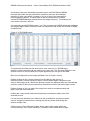
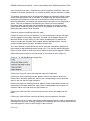
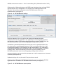
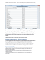
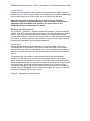
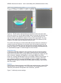
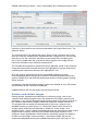
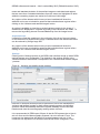
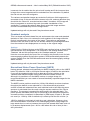
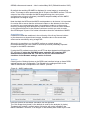
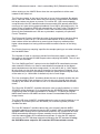
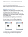
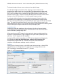
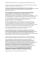
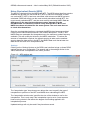
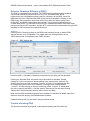
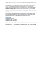
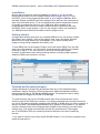
©DRIQ software and manual - John Loveland May 2015 (Edited November 2015)
Installation
Be sure that you have an existing installation of ImageJ. If you do not then
download and install it from the ImageJ website http://imagej.nih.gov/ij/. Copy
the DRIQ_.jar file to the ImageJ\plugins folder of your ImageJ installation. Note
that both ImageJ and DRIQ have been designed such that you can install and run
them from removable drives. To do so download the system independent version
of ImageJ and extract the zip file to your USB drive. Now navigate to the
ImageJ\plugins folder (within the newly extracted directory structure) and copy
the DRIQ_.jar file to this location. If you run the ImageJ version now residing on
you USB drive then DRIQ will be listed under the plugins menu.
Getting started
If ImageJ was already open when you installed DRIQ then you will need to refresh
the ImageJ menu options. Click on the ImageJ ‘Help’ menu and select ‘Refresh
Menus’ from the drop down menu that appears. If you did not already have
ImageJ running during installation then start it now.
To start DRIQ click on the ImageJ ‘Plugins’ menu and select ‘DRIQ’ from the drop
down menu that appears. You will now be presented with the DRIQ user interface
as shown in figure 1. You can continue to use all of the standard ImageJ
functions, measurement tools and processing options (including ImageJ plugins)
whilst the DRIQ user interface is running.
Figure 1 – DRIQ user interface
Opening and browsing images
Images and stacks of images can be opened using any of the standard ImageJ
interfaces if desired. However, DRIQ introduces an additional dedicated interface
designed specifically for DICOM and NEMA images. This allows the user to easily
sort and filter the images by DICOM or NEMA tags.
To use this facility click on the ‘DICOM browser with noise measurements’ button
at the top right of the DRIQ user interface. You will be presented with a browser which you
can use to navigate to the folder containing the DICOM or NEMA files you wish to analyse. A
dummy file name (“DICOMbrowserDefaultFile.tsv“) appears in the browser. If you want to
choose a directory leave this unchanged and navigate to the directory you want before
clicking okay. The system automatically includes any subfolders so if the images
are on a CDROM or DVD you need only direct the browser to the drive containing
the disc.
If you want to choose a previously saved DICOM browser (“.tsv”) file then navigate to this
saved file and select it.
©DRIQ software and manual - John Loveland May 2015 (Edited November 2015)
If a directory has been selected the program opens each DICOM and NEMA
file within this folder and any subfolders, measures the mean and standard
deviation of pixel value within a central roi (or an roi 6cm from chest wall for
mammography systems). A results table is then presented which includes
various DICOM/NEMA tags extracted from the images (figure 2). The directory the
user chose is shown in the title.
If a previously saved DICOM browser (“.tsv”) file is chosen then DRIQ opens and measures
the images slightly faster because it does not repeat the initial search for DICOM or NEMA
compliant files.
Figure 2- JL DICOM Browser
The horizontal scroll bar can be used to see more columns (i.e. DICOM tags)
whilst the vertical scroll bar can be used to see more rows. The file name appears in the
second column on the left whilst the full path appears at the far right of the table.
Each row corresponds to the image specified in the ‘Full path’ column.
Double clicking on any column header sorts the table by that column in
ascending order. Double clicking the same column header again changes the sort
order to descending order. Before the browser results are displayed they are automatically
sorted by study ID then series number then acquisition number and then image number.
Double clicking on any row opens the image from which the measurements and
tags in that row were extracted.
Holding the control button down whilst selecting rows allows multiple rows to be
selected at once.
If a row has been selected in the table then the up and down arrow keys can be
used to change the selected row. Holding the shift key down whilst doing this
selects multiple rows.
Clicking on the ‘Open selected images’ button opens each image within the
current selection. If the ‘Open as stack?’ checkbox is ticked then these images
©DRIQ software and manual - John Loveland May 2015 (Edited November 2015)
will be opened as a stack - otherwise they will be opened individually. Note only
images of the same dimensions (i.e. number of pixels) can be opened in a stack.
The bottom right hand corner of the browser displays a thumbnail (64x64) image
of the currently selected row in the table. If multiple rows are selected then the
thumbnail will correspond to the row in the selection closest to the top of the
table. By default the roi used for the measurements is shown on the thumbnail in
green. This can be hidden by de-selecting the ‘Show rois on thumbnails?’
checkbox. Note that because the thumbnails are always re-scaled to 64x64
pixels (whilst preserving aspect ratio) the roi may appear to be different sizes
depending upon which row is selected.
Control+A selects everything within the table
Control+C copies the current selection (i.e. the measurement results and tags not the images) to the system clipboard. The data can be pasted directly into
Microsoft Excel or Open Office or Libre Office spreadsheets. By default the
column headers are included in the copied data but deselecting the ‘Include
column headers when copying?’ checkbox will alter this.
The “Save Results” button allows the user to save the information displayed in
the browser in tab separated values format (.tsv). This can be read by Microsoft
Office or Libre Office or used to save time when re-opening the images in DRIQ.
Right clicking the mouse on any cell brings up a contextual menu (figure 3).
Figure 3 – JL DICOM Browser image filter
Clicking on Copy just copies the selected rows to the clipboard.
Clicking on ‘Keep matching records’ applies a filter to the table to show only
those rows in the table where the value in the corresponding column equal the
value in the cell that you right clicked on.
Clicking on ‘Remove matching records’ applies a filter to the table to show only
those rows in the table where the value in the corresponding column does not
equal the value in the cell that you right clicked on.
Clicking on ‘Undo last filter’ removes only the most recent filter applied to the
table.
Clicking on ‘Undo all filters’ removes all filters currently applied to the table.
Selecting the title of a column and clicking and dragging allows the user to rearrange the
ordering of the columns. Warning changes to the ordering are not currently saved for the
user although this is likely to be a facility in later versions.
Settings
©DRIQ software and manual - John Loveland May 2015 (Edited November 2015)
Clicking on the ‘Settings’ button on the DRIQ user interface brings up those DRIQ
options that are user configurable. The first tab in the settings section is the
‘Browser’ tab and this corresponds to the ‘DICOM browser with noise
measurements’ (see figure 4).
Figure 4 – JL DICOM Browser settings
Here the diameter of the roi used for the mean and standard deviation
measurements can be specified in mm separately for mammography systems
and all other systems. DRIQ automatically detects the system modality from the
DICOM headers and uses the mammography settings where relevant.
A checkbox (checked by default) also forces the roi to be positioned 6cm from
the chest wall on mammography systems. If this in unchecked then the roi will
be positioned centrally in the image as with all other systems. The chest wall is
automatically identified using the laterality tag in the DICOM header of files with
modality=”MG”. DRIQ automatically detects the system modality from the
DICOM headers and uses the mammography settings where relevant.
A second checkbox will use the IEC standard rois for STP measurement if checked
(100x100 pixel square roi).
Updated settings will only be used if they have been saved.
Clicking on the “Edit output DICOM tags” allows the user to specify the DICOM
tags that will be included in the DICOM browser window (see figure 5).
Figure 5 – JL DICOM Browser output options
©DRIQ software and manual - John Loveland May 2015 (Edited November 2015)
Here the user can add and remove the DICOM tags included in the DICOM
Browser by using the buttons “Add New Row” and “Delete Row”. The tags can be
specified separately for DR and CR, mammography, and CT modalities using the
drop down menu at the top of the window. DRIQ automatically detects the
modality from the DICOM headers and uses the relevant output settings. To close
the editor simply use the close window icon in the top right hand corner of the
window.
Updated settings will only be used if they have been saved.
Making measurements – Before beginning
The DICOM browser makes some basic roi measurements which can be used for
determining the noise characteristics, the detector SNR, and the Signal Transfer
Property (STP) for the system. If using the IEC standard methods for
analysis then follow the relevant IEC standards when acquiring the
images and linearising them. Also ensure that the “Use IEC roi for STP
measurements?” checkbox in the Browser settings section is ticked.
Measuring the STP
Exposures must be made with known values of incident air kerma to the
detector across a range of clinical air kerma values (see IPEM report 32
part vii for further details).
Plot the mean pixel value (as output from the DICOM browser) vs the
incident air kerma
Perform an appropriate fit to the plotted data (e.g. linear, logarithmic or
power law).
©DRIQ software and manual - John Loveland May 2015 (Edited November 2015)
Linearisation
Images should be linearised before further measurements are made. Enter the
factors from your STP fit into the DRIQ user interface and choose the system type
from the drop down menu at the center top of the DRIQ user interface.
Each time an image or stack of images is opened for the first time
select the image or stack and then click on the ‘Linearise’ button at the
right hand side of the DRIQ user interface. The pixel values in the
image should now correspond to air kerma.
Making measurements
The ‘Linearise’, ‘Uniformity’, ‘Variance and artefact Images’, ‘Quadrant Analysis’,
‘NNPS’, and ‘MTF’ buttons all apply operations to the currently selected image in
ImageJ. The currently selected image in ImageJ is the image that has most
recently been opened or clicked upon. Be sure that you have selected the image
upon which you wish to perform the measurement and that this image has been
linearised as described in the preceding paragraphs.
Uniformity
Having opened, selected and linearised your uniformity image click on the
‘Uniformity’ button. By default a 1cm region around each edge of the image is
excluded from the uniformity calculation. If you use the standard ImageJ tools to
draw an roi before clicking on the ‘Uniformity’ button then DRIQ will instead use
this roi.
The program will now perform measurements of the mean and standard
deviation of pixel values (i.e. incident air kerma) within a sub-roi at multiple
points within the user selected or default roi. A 3D plot of the mean pixel values
will be displayed and the user selected or default roi will be shown on the original
uniformity image. Areas that fail the remedial tolerance for uniformity will be
highlighted in orange on the original image whilst areas that fail the suspension
tolerance will be highlighted in red on the original image. The colours on the 3D
plot are not related to the tolerance levels.
Figure 6 – Example of uniformity output
©DRIQ software and manual - John Loveland May 2015 (Edited November 2015)
Figure 6 – The 3D- plot on the left shows the variation in the mean pixel value
across the chosen roi. Use the Max and Min sliders to change the maximum and
minimum values to be displayed on the 3D plot. The yellow rectangle on the
right shows the user selected or default roi used for the assessment. The solid
orange square within this rectangle shows that this area of the detector (in this
instance a CR plate) failed the remedial tolerance level.
The routine also brings up a small results table which provides the coefficient of
variation across the uniformity roi, the mean of all of the means from each sub
roi, the maximum deviation from this value and the maximum deviation from the
mean of a central roi. The data from this table can be copied and pasted directly
to a spreadsheet progam or saved straight to a file of its own.
Acquisition tips
It should be noted that variations in the uniformity of the X-ray fluence incident
on the detector will also appear in this image. Variations due to the anode-heel
effect can be reduced by using a large SID and/or averaging two images with the
tube or detector rotated by 180 degrees in one image relative to the other
image. An “Average DICOM stack” button is provided in DRIQ for this purpose. To
use it, open the images you wish to average as a stack in ImageJ. Select this
stack and then click the “Average DICOM stack” button in DRIQ. The resulting
average DICOM image will contain the DICOM header information from the first
slice in the stack.
Settings
Clicking on the ‘Settings’ button on the DRIQ user interface brings up those DRIQ
options that are user configurable. The second tab in the settings section is the
‘Uniformity’ tab and this corresponds to the ‘Uniformity ’ process .
Figure 7- Uniformity process settings
©DRIQ software and manual - John Loveland May 2015 (Edited November 2015)
Here the roi size used for the uniformity calculation can be specified in mm. The
default is 20mm.
The increment size is by default also set to 20mm. If this is equal to the roi size
then the uniformity measurement is performed with contiguous rois. If this is less
than the roi size the uniformity calculation is performed with overlapping sub
rois. If this is greater than the roi size then some regions of the image will not
have been included in the uniformity measurement.
The remedial and suspension tolerances can be adjusted. Areas in the uniformity
image that exceed the remedial tolerance are highlighted in orange whilst areas
exceeding the suspension tolerance are highlighted in red.
All of the settings mentioned so far are changeable separately for both
mammography systems and all other systems. DRIQ automatically detects the
system modality from the DICOM headers and uses the mammography settings
where relevant.
A checkbox (checked by default) allows control over whether or not a 3D surface
representation of the uniformity is displayed.
Updated settings will only be used if they have been saved.
Variance and artefact images
Having opened, selected and linearised your uniformity image, click on the
‘Variance and artefact Images’ button. By default the full image is used for the
calculation. If you use the standard ImageJ tools to draw an roi before clicking on
the ‘Variance and artefact Images’ button then DRIQ will instead use this roi.
The program will now perform measurements of the mean, variance, and
standard deviation of pixel values (i.e. incident air kerma) within a sub-roi at
multiple points within the user selected or default roi. A new image – the
variance image - will be created and displayed using the variance from each subroi.
Regions with a variance more than three times the average variance in the
image are shown highlighted in white whilst the remaining regions are scaled to
fit within an 8-bit image. A second image – the artefact image- will also be
created and displayed showing the standard deviations from each sub-roi. The
©DRIQ software and manual - John Loveland May 2015 (Edited November 2015)
mean and standard deviation of the artefact image are calculated and regions
that are more than 3 standard deviations from this mean are highlighted in white
whilst the remaining regions are scaled to fit within an 8-bit image.
Any regions of the detector which have not been irradiated will skew the
statistics and a user roi should be specified that excludes these regions before
clicking on the ‘Variance and artefact Images’ button.
An option is available to view the un-scaled variance matrix for the image. If
enabled this is displayed on a natural log scale so that variations are visible. To
remove the log scaling choose Process>Math>Exp from the ImageJ menu.
Acquisition tips
It should be noted that variations in the uniformity of the X-ray fluence incident
on the detector may impact these image. Variations due to the anode-heel effect
can be reduced by using a large SID.
Any regions of the detector which have not been irradiated will skew the
statistics and a user roi should be specified that excludes these regions before
clicking on the ‘Variance and artefact Images’ button.
Settings
Clicking on the ‘Settings’ button on the DRIQ user interface brings up those DRIQ
options that are user configurable. The third tab in the settings section is the
‘Variance/artefact’ tab and this corresponds to the ‘Variance and artefact Images
’ process.
Figure 8 – Variance and artefact image settings
Here the roi size and increment can be specified in mm for the calculation of
variance and artefact images for both mammography systems and all other
systems. DRIQ automatically detects the system modality from the DICOM
headers and uses the mammography settings where relevant.
It is recommended in IPEM report 32 part vii that for DR systems the roi size is
set to 2.0mm and for Mammography systems it is set to around 0.7mm. The
increment size determines the degree of overlap between sub rois. If the
increment size equals the roi size then the sub rois will be contiguous. If the
©DRIQ software and manual - John Loveland May 2015 (Edited November 2015)
increment size is smaller then the sub rois will overlap and if the increment size
is larger then some image data will be excluded from the calculation. By default
the sub rois are set to be contiguous.
The variance and artefact images are scaled to fit within an 8-bit image and so
some data is lost. If the user would like access to the full variance data then they
should tick the ‘Show full, unscaled variance data?’ checkbox. A 2D image will
then be presented on a natural log scale (to enable visualisation of the
variations). To restore the variance data simply select this image and then
choose Process>Math>Exp from the ImageJ menu.
Updated settings will only be used if they have been saved.
Quadrant analysis
This is a simple tool which draws five rois and measure the mean and standard
deviation of each. One roi is centered in each quadrant of the image whilst the
final roi is positioned in the centre of the image. The maximum percentage
deviation from the mean of the five rois and the maximum percentage deviation
from the central rois are displayed as an overlay on the original image.
Settings
Clicking on the ‘Settings’ button on the DRIQ user interface brings up those DRIQ
options that are user configurable. The fourth tab in the settings section is the
‘Quadrant’ tab and this corresponds to the ‘Quadrant analysis ’ process.
Here the user can specify the size of the roi used for this process in mm for both
mammography systems and all other systems. DRIQ automatically detects the
system modality from the DICOM headers and uses the mammography settings
where relevant.
Updated settings will only be used if they have been saved.
Normalised Noise Power Spectrum (NNPS)
Having opened, selected and linearised your NNPS image(s) click on the ‘NNPS’
button. By default a 1024 by 1024 pixel central region is used for the calculation.
If you use the standard ImageJ tools to draw an roi before clicking on the
‘Variance and artefact Images’ button then DRIQ will instead use this roi.
Although it is possible to run the NNPS routine on a single image it is
recommended that you use a stack of several identically exposed images for the
NNPS calculation.
The NNPS routine positions small rois (128 by 128 default) at various locations
throughout the default or user selected roi. A two dimensional polynomial
surface is fitted and subtracted from each individual sub-roi and then the power
spectrum is calculated from the result using the square modulus of the Fourier
transform. The process is repeated for each image in the selected stack. The
power spectra calculated in this way for each sub roi and across all images are
summed and then normalised. As described in IPEM report 32 part vii, the main
rois used (i.e. 1024 by 1024 for default roi) is offset by half the sub roi size (i.e.
128/2 for default) in each stack in both the x and y directions. However, since
this recommendation could lead to rois extending beyond the image edges for
large stacks then in such an instance the routine will instead offset each main roi
by a random displacement (from –N/2 to +N/2 where N= sub roi size) in the x
and y directions .
©DRIQ software and manual - John Loveland May 2015 (Edited November 2015)
By default the resulting 2D NNPS is displayed in a new image on a natural log
scale. This image is also represented with a 3D plot of the NNPS surface. The text
output of the routine includes the NNPS sampled along the x and y axes
(excluding the u=0 and v=0 values), the NNPS sampled radially and the NNPS
sampled at a 45 degree angle.
Note that both the NPS and the NNPS are dependent on air kerma. It is important
for routine QA to ensure that the air kerma incident on the detector is the same
as used for your commissioning data. It is possible to scale to a reference air
kerma by multiplying each data point by K/Kref where K is the air kerma incident
on the detector and Kref is the reference air kerm to which you wish to scale.
See IPEM report 32 part vii for further information about the calculation of NNPS.
Acquisition tips
It should be noted that variations in the uniformity of the X-ray fluence incident
on the detector may impact these images. Variations due to the anode-heel
effect can be reduced by using a large SID.
Although it is possible to run the NNPS routine on a single image it is
recommended that you use a stack of several (at least 4) identically exposed
images for the NNPS calculation.
If using the IEC method ensure that your STP has been determined following the
IEC standard. If using the DICOM browser output for IEC standard STP
determination ensure that the “Use IEC roi for STP measurements?”
checkbox in the Browser settings section is ticked.
Settings
Clicking on the ‘Settings’ button on the DRIQ user interface brings up those DRIQ
options that are user configurable. The fifth tab in the settings section is the
‘NNPS’ tab and this corresponds to the ‘NNPS ’ process.
Figure 9 – NNPS settings tab
Here the options for the NNPS calculation can be specified.
The ‘Sub image size (pixels)’ is the default roi used for the analysis (in pixels).
The data lying outside a central region of this size will not be included in the
NNPS calculation. However, if an ImageJ roi has already been drawn by the user
©DRIQ software and manual - John Loveland May 2015 (Edited November 2015)
before clicking on the ‘NNPS’ Button then the user specified roi will be used
instead of this default roi.
The ‘Roi size (pixels)’ is the size of the sub roi to use for the analysis. By default
this is 128x128. Small values distort the low frequency components of the NNPS
but larger values are slower to process. For routine QC, 128 is an acceptable
compromise but the IEC standard method recommends 256 (actually with DRIQ
running on a 8 year old low powered netbook I found 256 is still pretty quick). If a
power of two is used then DRIQ will automatically use Fast Fourier Transforms to
speed up computation time. If a power of two is not used then the processing
time may be considerable as it will use my standard, completely un-optimised
Fourier Transform.
The ‘Polynomial fit order’ specifies the order of the polynomial to use when fitting
a 2D surface to each sub roi. It is recommended that this is left at 2 because
lower values will be less effective at removing low frequency artefacts whilst
higher values depend on having sufficient data to enable inversion of the fitting
matrix.
The ‘Re-bin frequency sampling’ specifies the sample spacing to use when rebinning
the final NNPS data.
The ‘Number of rows or columns to extract from frequency space’ is the width of
the profile to use through 2D NNPS space when sampling the NNPS. The u=0 and
v=0 data are excluded.
The ‘Use ObjIQ type Rois?’ option mimics the ObjIQ NPS normalisation process
when selected. Here the roi used for normalisation corresponds to the largest
area sampled across the whole image stack (i.e. this will be M+ (x-1)*N/2 where
M is the main roi size, N is the sub roi size and x is the number of images). If it is
de-selected then the NPS normalisation divides the power spectrum by the mean
of the main roi (i.e. 1024x1024 for default roi) size in each image.
The ‘Use overlapping Rois?’ checkbox allows the user to specify whether the sub
rois should overlap or be contiguous. If the rois are set to overlap then they will
overlap by N/2 where N is the sub roi size. It is recommended that this remains
ticked.
The ‘Show full 2D NNPS?’ checkbox allows the user to specify whether or not the
2D NNPS will be displayed. If it is checked then the 2D NNPS will be displayed on
a natural log scale to enable visualisation of variations. To restore the original
NNPS data select the 2D NNPS and then choose Process>Math>Exp from the
ImageJ menu.
The ‘Show 3D view of NNPS?’ checkbox allows the user to specify whether or not
to display a 3D surface plot of the 2D NNPS (on a natural log scale) to better
visualise the data.
The ‘Use IEC Method?’ checkbox allows the user to specify that the NNPS
calculation should be performed using the IEC method. If this is checked then the
standard NNPS settings will be ignored and instead the IEC method will be used.
DRIQ automatically detects the system modality from the DICOM headers and
uses the mammography IEC method where relevant. If using the IEC method
ensure that your STP has been determined following the IEC standard. If using
the DICOM browser output for IEC standard STP determination ensure
©DRIQ software and manual - John Loveland May 2015 (Edited November 2015)
that the “Use IEC roi for STP measurements?” checkbox in the Browser
settings section is ticked.
If using the IEC method for NNPS in DRIQ then DRIQ will automatically provide warnings if
you require more images to meet the IEC standard requirements
Similarly if the variance between images falls outside of the IEC requirements DRIQ will alert
the user automatically.
Updated settings will only be used if they have been saved.
Modulation Transfer Function (MTF)
The default MTF routine in DRIQ uses the edge finding methods of the IEC standard
combined with custom routines to detected outliers (e.g. dead pixels, dust, interpolation
artefacts). In this way the edge is angle is found with a precision of at least 0.01 degrees
(verified in the range 0.2 to 15.3 degrees). The MTF calculation is then performed following
the oversampling methodology of Samei, Flynn and Reimann (1998).
DRIQ will specify how many outliers were discarded in the output and it is good
practice to visually inspect those edge images containing discarded pixels. Be sure to
zoom in and adjust the window and level to check for interpolation artefacts and dead pixels
in the MTF roi. The MTF calculation will still be performed but if the artefact is significant you
may wish to highlight it clinically.
When acquiring your MTF image, for best results the edge test object should be
aligned at an angle between 2 and 5 degrees to the pixel matrix (IPEM report 32
part vii) or 1.5 to 3 degrees for IEC standard.
Having opened, selected and linearised your MTF image use the standard ImageJ
tools to draw a rectangular roi over the edge in the image. Edges aligned along
the vertical axis of the image provide the horizontal MTF whilst edges aligned
along the horizontal axis provide the vertical MTF (see figure 10). This is because
the ESF is sampled along the direction perpendicular to the edge.
Figure 10- Modulation Transfer Function process
Horizontal MTF
Vertical MTF
Click on the ‘MTF’ button. The roi you drew is resized to the default size in mm as
specified in the DRIQ settings. If the edge is detected but the roi you drew was
not central enough to the edge then DRIQ will move the roi appropriately and
request that you try running the MTF routine again in this new position.
©DRIQ software and manual - John Loveland May 2015 (Edited November 2015)
The detected edge is shown as an overlay on the original image.
The calculated angle and location of the edge are used to determine the
distances from each pixel in the roi to the edge. This distance data is then used
to bin the pixel data to attain the oversampled Edge Spread Function (ESF). The
ESF is then smoothed using a median filter and differentiated to obtain the Line
Spread Function (LSF). The MTF is finally calculated as the modulus of the Fourier
transform of the LSF normalised to 1.0 at the spatial frequency origin.
An optional additional iterative loop is provided to attempt to further reduce the
uncertainties in the edge angle. If enabled the loop calculates the integral of the
MTF up to the Nyquist frequency using 200 different edge angles around the calculated
value. The angle returning the maximum value of the integral is then used for the
determination of the full MTF. This process should be used with caution as aliasing effects
may provide higher integral values than the true presampling MTF.
Acquisition tips
It should be noted that variations in the uniformity of the X-ray fluence incident
on the detector may impact these image. Variations due to the anode-heel effect
can be reduced by using a large SID.
When acquiring your MTF image, for best results the edge test object should be
aligned at an angle between 2 and 5 degrees to the pixel matrix (IPEM report 32
part vii) or 1.5 to 3 degrees for IEC standard.
If using the IEC method ensure that your STP has been determined following the
IEC standard. If using the DICOM browser output for IEC standard STP
determination ensure that the “Use IEC roi for STP measurements?”
checkbox in the Browser settings section is ticked.
Settings
Clicking on the ‘Settings’ button on the DRIQ user interface brings up those DRIQ
options that are user configurable. The sixth tab in the settings section is the
‘MTF’ tab and this corresponds to the ‘MTF ’ process.
Figure 11 – MTF process settings
©DRIQ software and manual - John Loveland May 2015 (Edited November 2015)
Here the roi size to use can be specified in mm. By default this is 68.75mm to match the
enlarged roi ObjIQ uses for a 50mm nominal roi.
The ‘Number of samples to take from Edge Spread Function’ must be large
enough to provide a decent profile across the edge but small enough that there are sufficient
data points in each bin. Larger values will require more processing time. By
default this is set to 1024.
The ‘Oversample factor’ is used to determine the sample spacing for re-binning
the oversampled ESF. By default this is set to 10 which means that the sample
spacing used will be 10 times smaller than the image pixel size. If the
oversample factor is set to be too large then some bins within the re-sampled
ESF will be empty and the routine will warn the user and attempt to interpolate these bins. If
the oversample factor is too small then then sampling of the MTF may be too coarse.
The ‘Re-bin frequency sampling’ specifies the sample spacing to use when rebinning
the final calculated MTF. This does not affect the full frequency data
provided in the output – only the re-binned data.
‘Number of samples to process in FFT’ specifies how may samples to use from
the over sampled ESF for the calculation of the MTF. Too low a value and the ESF
may not be completely represented, too high a value and the computational time
may be high. If the value is a power of two then the system uses a Fast Fourier Transform
routine but if it is not a power of two then a much slower algorithm will be used.
The ‘Iteratively optimise MTF over low frequencies?’check box enables the
iterative edge angle optimisation described earlier and below:
“An optional additional iterative loop is provided to attempt to further reduce the
uncertainties in the edge angle. If enabled the loop calculates the integral of the
MTF up to the Nyquist frequency using 200 different edge angles around the calculated
value. The angle returning the maximum value of the integral is then used for the
determination of the full MTF. This process should be used with caution as aliasing effects
may provide higher integral values than the true presampling MTF.”
The ‘Window size for median filter’ specifies the extent of the median smoothing
applied to the ESF before differentiation. By default this matches the ObjIQ default.
The ‘Use IEC Method?’ checkbox allows the user to specify that the MTF
calculation should be performed using the IEC method. If this is checked then the
standard MTF settings will be ignored and instead the IEC method will be used
(this is a completely different methodology for sampling the ESF and is described well in
Buhr,Gunther-Kohfahl and Neitzel (2003). DRIQ automatically detects the system
modality from the DICOM headers and uses the mammography IEC method
where relevant. It is important to acquire the edge image using the IEC
methodology if the IEC checkbox is ticked. This also means using an IEC standard
edge. If using the IEC method ensure that your STP has been determined
following the IEC standard. If using the DICOM browser output for IEC
standard STP determination ensure that the “Use IEC roi for STP
measurements?” checkbox in the Browser settings section is ticked.
Updated settings will only be used if they have been saved.
©DRIQ software and manual - John Loveland May 2015 (Edited November 2015)
Noise Equivalent Quanta (NEQ)
The NEQ is calculated from the NNPS and MTF. The NEQ button therefore remains
disabled until at least one horizontal MTF (MTFu) has been calculated, at least
one vertical MTF (MTFv) has been calculated, and at least one NNPS has been
calculated. DRIQ will simply use the most recently calculated vertical MTF, the
most recently calculated MTF, and the most recently calculated NNPS. Due to
differences in the way that manufacturers store detector ID in the
DICOM header no checks are made to verify that the MTFu, MTFv and
NNPS have been calculated for the same system. The user must be sure
to check this themselves.
Once the required data has been calculated the NEQ button becomes enabled.
Clicking on the NEQ button produces a list of NEQ data points. The MTF and
NNPS data are resampled and interpolated up to the maximum spatial frequency
available. This will usually be limited by the NNPS calculation. To reduce the
amount of interpolation required, the sample spacing is taken as the smallest
spacing between data points in the MTF and NNPS data such that at least one
data set will not have to be interpolated at all.
Settings
Clicking on the ‘Settings’ button on the DRIQ user interface brings up those DRIQ
options that are user configurable. The seventh tab in the settings section is the
‘NEQ’ tab and this corresponds to the ‘NEQ’ process.
Figure 12 – NEQ settings tab
The ‘Interpolation type’ drop down menu allows the user to specify the type of
interpolation to perform on the MTF and NNPS when calculating the NEQ.
The ‘Interpolation window size’ specifies the size of the window to use for the
interpolation. This is only used if the interpolation type is set to ’Least squares
linear moving window’ and affects the degree of smoothing applied in the
interpolation process.
Updated settings will only be used if they have been saved.
©DRIQ software and manual - John Loveland May 2015 (Edited November 2015)
Detector Quantum Efficiency (DQE)
The DQE is calculated from the NEQ. The DQE button therefore remains disabled
until at least one NEQ process has been run. The calculated DQE will be
influenced by the interpolation options used for calculation of the NEQ. Once the
NEQ data has been calculated the DQE button becomes available. Clicking on the
DQE button then provides a drop down menu from which the beam quality used
for the MTF and NNPS images must be selected. The routine then produces a list
of DQE data points. For the DQE to follow the IEC standard the NNPS must have been
performed using the IEC standard, and the MTF must have been determined using the IEC
standard in both horizontal and vertical directions.
Settings
Clicking on the ‘Settings’ button on the DRIQ user interface brings up those DRIQ
options that are user configurable. The eighth tab in the settings section is the
‘DQE’ tab and this corresponds to the ‘DQE’ process.
Figure 13 – DQE settings tab
Here the SNR2 in_Q (Number of photons per square mm per μGy) can be specified.
Clicking on ‘Add New Row’ will add a row to the bottom of the table. Double
clicking in a cell in the new row allows editing of the values within that cell. E.g.
double clicking on the Cell containing “Custom” in figure 13 would allow the user
to change the System name to for example “Charing Cross hospital Room2
+1mmCu”. Double clicking on the cell containing “6242” in figure 13 would allow
the user to specify the SNR2 in_Q for this system. Selecting a row and then clicking
‘Delete Row’ will permanently remove that row from the table.
Note that the RQA and Mammography beam qualities in the table by default cannot be
edited or removed as they are standard beam qualities.
Updated settings will only be used if they have been saved.
Trouble shooting/FAQ
The browser will show its progress in parsing and opening the files within the
©DRIQ software and manual - John Loveland May 2015 (Edited November 2015)
selected directory in the status area of ImageJ at the bottom left hand corner of
ImageJ. If this appears to have stopped increasing then it is likely that the
browser has encountered a file which only partially follows the DICOM or NEMA
standards and which I haven't already written code to handle. Try removing this
file and attempting again.
Clicking on the ImageJ status area and then pressing escape will abort the active
process.
Sometimes you may wish to perform measurements on images without DICOM
tags or with tags missing. It may then be necessary to use the Pixel size box on
the DRIQ user interface to manually specify the pixel size in mm.
References
IPEM report 32 part vii
IEC 62220-1-2 Ed. 1.0 b 2007
IEC 62220-1 Ed. 1.0 en 2003
ObjIQreducedV2 user manual
Buhr E., Gunther-Kohfahl S., and Neitzel U., Medical Physics, Vol. 30, No. 9, 2003
Samei E, Flynn M. J., and Reimann D.A., Medical Physics, Vol. 25, No 102,1998