Download Untitled - CLC bio

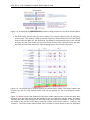
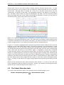
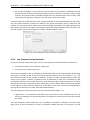
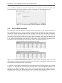
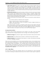
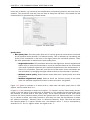
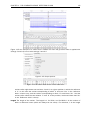
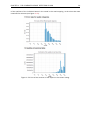
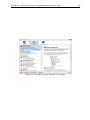
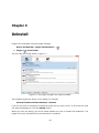
User manual for
Combined Variant Detection Beta Plugin
1.0
Windows, Mac OS X and Linux
April 25, 2014
This software is for research purposes only.
CLC bio, a QIAGEN Company
Silkeborgvej 2
Prismet
DK-8000 Aarhus C
Denmark
Contents
1 The Combined Variant Detection plugin
4
1.1 Introduction . . . . . . . . . . . . . . . . . . . . . . . . . . . . . . . . . . . . . .
4
1.2 The Variant Detection tools . . . . . . . . . . . . . . . . . . . . . . . . . . . . . .
6
1.2.1 Basic Variant Detection . . . . . . . . . . . . . . . . . . . . . . . . . . . .
8
1.2.2 Fixed Ploidy Variant Detection . . . . . . . . . . . . . . . . . . . . . . . . .
8
1.2.3 Low Frequency Variant Detection . . . . . . . . . . . . . . . . . . . . . . .
9
1.2.4 The Error Model estimation . . . . . . . . . . . . . . . . . . . . . . . . . .
10
1.3 The filters . . . . . . . . . . . . . . . . . . . . . . . . . . . . . . . . . . . . . . .
11
1.3.1 General filters . . . . . . . . . . . . . . . . . . . . . . . . . . . . . . . . .
11
Reference masking . . . . . . . . . . . . . . . . . . . . . . . . . . . . . .
11
Read filters
. . . . . . . . . . . . . . . . . . . . . . . . . . . . . . . . . .
11
Coverage and count filters . . . . . . . . . . . . . . . . . . . . . . . . . .
12
1.3.2 Noise filters . . . . . . . . . . . . . . . . . . . . . . . . . . . . . . . . . .
12
Quality filters . . . . . . . . . . . . . . . . . . . . . . . . . . . . . . . . . .
13
Direction and position filters . . . . . . . . . . . . . . . . . . . . . . . . .
14
Technology specific filters . . . . . . . . . . . . . . . . . . . . . . . . . . .
16
1.4 Output options . . . . . . . . . . . . . . . . . . . . . . . . . . . . . . . . . . . . .
17
1.4.1 The variant track output . . . . . . . . . . . . . . . . . . . . . . . . . . . .
17
1.4.2 The annotated table output . . . . . . . . . . . . . . . . . . . . . . . . . .
20
1.4.3 The report . . . . . . . . . . . . . . . . . . . . . . . . . . . . . . . . . . .
20
2 Installation of the Combined Variant Detection
22
3 Uninstall
24
Bibliography
25
3
Chapter 1
The Combined Variant Detection plugin
1.1
Introduction
The Combined Variant Detection plugin contains three tools for detecting variants:
• The 'Basic Variant Detection' tool
• The 'Fixed Ploidy Variant Detection' tool and
• The 'Low Frequency Variant Detection' tool
The tools differ in their underlying assumptions about the data, and hence differ in their
assessments of when there is enough information in the data for a variant to be called. The
tools, and the assumptions that they make about the data, are described in detail in Section 1.2.
The tools share a set of filters. They relate to (a) which areas and positions of the read mappings
that should be inspected for variants, (b) which reads in the data should be considered when
this assessment is done, (c) requirements to the coverage, frequency and absolute counts of
variant carrying reads and (d) the quality and neighborhood composition of the area surrounding
the variant. The filters are described in detail in Section 1.3.
The variant callers operate in a step-wise fashion. In the first step each nucleotide positions
is examined for the presence of a variant, in the second step neighboring variant positions are
examined to see if the variants are carried by the same reads. If so, the variants are joined
(neighboring SNVs into MNVs, neighboring insertions and deletions into longer insertions and
deletions, and neighboring SNVs and insertions or deletions into replacements). The filters are
applied at various stages - some before the initial 1 bp variants are found, and some after.
Figure 1.1 shows a schematic representation of the procedure.
As the tools differ in their model assumptions about the data, they will not call the same variants.
However, when run with the same filter settings, you will generally have that:
• The Basic Variant Caller will call the highest number of variants
• The Low Frequency Variant Caller will call a subset of the variants called by the Basic Variant
caller. The variants called by the Basic Variant Caller that the Low Frequency Variant Caller
will NOT call, are those that, according the error model that the Low Frequency Variant
Caller estimates from the data, are likely to have been caused by sequencing errors.
4
CHAPTER 1. THE COMBINED VARIANT DETECTION PLUGIN
5
Figure 1.1: A schematic representation of the variant calling procedure of the three variant callers.
• The Fixed Ploidy Variant Caller will call a subset of the variants called by the Low Frequency
Variant caller. The variants called by the Low Frequency Variant Caller that the Fixed Ploidy
Variant Caller will NOT call, are those that, according to the assumed ploidy of the sample
analyzed and the error model that the Fixed Ploidy Variant Caller estimates from the data,
are likely to have been caused by either mapping errors or by sequencing errors.
Figure 1.2: The differences in variants called by the three variant callers. The variant callers have
all been run with the filter settings (those that are the defaults for the Low Frequency Variant
Caller).
Figure 1.2 shows variant calls produced by the three variant callers when run with the same filter
settings, more precisely those that are default for the Low Frequency Variant Caller. The Basic
Variant Caller calls most variants and the Fixed Ploidy the least (the numbers of called variants
are shown in the left part of the figure, under the variant track names 'basicV2', 'LowFreq' and
'FixedV2'). The Fixed Ploidy Variant Caller calls a subset of those called by the Low Frequency
CHAPTER 1. THE COMBINED VARIANT DETECTION PLUGIN
6
Variant caller, which in turn calls a subset of those called by the Basic Variant caller --- in spite
of the fact that there are 9 variants in the Low Frequency variant track that are not in the Basic
Variant track. Although those 9 variants are in fact not in the Basic Variant track, they are
'sub-variants' of variants in that track. The highlighted variants in the figure is an example of
this: The Basic variant caller has called a heterozygous 2bp MNV. The Low Frequency variant
caller has judged that one on the SNVs constituting this 2bp MNV is likely to be the result of
sequencing errors, and has only called one of the SNVs.
Figure 1.3: A variant is highlighted that is detected by the Basic Variant Caller but not by the Low
Frequency or the Fixed Ploidy Variant Caller. The variant track for the Basic variant Caller variants
is opened in the table-view at the bottom of the figure. The variant is present at a low frequency in
a high coverage position, and is likely to have been caused by sequencing error.
In figure 1.3 a variant is highlighted that is detected by the Basic Variant Caller but not by the Low
Frequency or the Fixed Ploidy Variant Caller. The variant is present at a low frequency in a high
coverage position. The Low Frequency Variant Caller compares this evidence to the error model,
and has decided that the three reads carrying the variant are likely to be the result of sequencing
errors, rather than the result of a true variant. Figure 1.4 highlights a variant that is detected
by both the Basic and the Low Frequency Variant Caller, but not the Fixed Ploidy. The variant is
present at a higher frequency (14.22%) in a high coverage region (coverage 204). Observing the
variant in 29 out of 204 reads is not likely to be due to sequencing errors. However, observing 29
reads from one allele and the remaining from the other in a diploid sample is highly unlikely, and
the Fixed Ploidy Variant Caller judges that this variant is most likely caused by mapping errors
(that is, a subset of the reads in the region being mapped there spuriously) and filters out this
variant.
Below we first describe the three variant detection tools (Section 1.2). Each of the tools have
a set of parameters that are specific to that tool. Second, we describe the filtering and output
options that are shared among the tools (Section 1.3).
1.2
The Variant Detection tools
To run the Variant Detection tools in the Combined Variant Detectionplugin, go to:
Toolbox | Resequencing Analysis (
) | Variant Detectors (beta)
CHAPTER 1. THE COMBINED VARIANT DETECTION PLUGIN
7
Figure 1.4: A variant is highlighted that is detected by the Basic and the Low Frequency but not by
the Fixed Ploidy Variant Caller. The variant track for the Low Frequency Variant Caller variants is
opened in the table-view at the bottom of the figure. The variant is present at a moderate frequency
in a high coverage position, and is, under the assumed ploidy, most likely to have been caused by
mapping error.
Here you are presented with the three tools (see figure 1.5).
Figure 1.5: The Variant Detectors.
When double-clicking one of the tools, a dialog is opened where you select the reads track or
read mapping you want to analyze.
Figure 1.6: Select the read mapping that you want to analyze.
Click Next when the reads track is listed in the right-hand side of the dialog.
The user is next asked to set the parameters that are specific for the variant detection tool. The
three tools, their assumptions, and the tool-specific parameters are described here:
CHAPTER 1. THE COMBINED VARIANT DETECTION PLUGIN
1.2.1
8
Basic Variant Detection
The Basic Variant Detection tool does not rely on any assumptions on the data, and does not
estimate any error models. It can be used on any type of sample. It will call a variant if it satisfies
the requirements that you specify when you set the filters (see Section 1.3). The tool has a
single parameter (Figure 1.7) that is specific to this tool: the user is asked to specify the 'ploidy'
of the sample that is being analyzed. The value of this parameter does not have an impact
on which variants are called - it will merely determine the contents of the 'hyper-allelic' column
that is added to the variant track table: variants that occur in positions with more variants than
expected given the specified ploidy, will have 'Yes' in this column, other variants will have 'No'.
Figure 1.7: The Basic Variant Detection parameters.
1.2.2
Fixed Ploidy Variant Detection
The Fixed Ploidy Variant Detection tool relies on two models:
1. a model for the possible 'site-types' and
2. a model for the sequencing errors.
The model for the possible 'site-patterns'((i)) depends on the user-specified ploidy parameter:
For a diploid organism there are two alleles and thus the site types are A/A, A/C, A/G, A/T,
A/-, C/C, and so on until -/-. The error model, (ii), specifies the probabilities of the analyzed
sample having a certain base in the sequenced position, but a different base being called in a
read at that position. The error model is estimated from the data prior to calling the variants
(see Section 1.2.4). The Fixed Ploidy algorithm will, given the estimated error model and the
data observed in the site, calculate the probabilities of each of the site types. One of those
site types is the site that is homozygous for the reference - that is, it stipulates that whatever
differences are observed from the reference nucleotide in the reads is due to sequencing errors.
The remaining site-types are those which stipulate that at least one of the alleles in the sample
is different from the reference. The sum of the probabilities for these latter site types is the
posterior probability that the sample contains at least one allele that differs from the reference
at this site.
The Fixed Ploidy Variant Detection tool has two parameters: the 'Ploidy' and the 'Variant
probability' parameters (Figure 1.8):
• The 'ploidy' is the ploidy of the analyzed sample. The value that the user sets for this
parameter determines the site types that are considered in the model.
CHAPTER 1. THE COMBINED VARIANT DETECTION PLUGIN
9
• The 'variant probability' is the minimum value required for the posterior probability that the
sample contains at least one allele that differs from the reference at this site, before calling
a variant. Only variants with a probability higher than the specified value will be called. That
means that the higher the value you set, the fewer variants are called.
As the Fixed Ploidy Variant Detection tool strongly depends on the model assumed for the ploidy,
the user should carefully consider the validity of the ploidy assumption that he makes for his
sample. The tool allows ploidy values up to and including 4 (tetraploids). For higher ploidy values
the number of possible site types is too large for estimation and computation to be feasible, and
the user should use the Low Frequency or Basic Variant Detection Tools.
Figure 1.8: The Fixed ploidy Variant Detection parameters.
1.2.3
Low Frequency Variant Detection
As the Fixed Ploidy Variant Detection tool, the Low frequency variant Detection tool relies on
1. a statistical model for the analyzed sample and
2. a model for the sequencing errors.
The method employed in the Low Frequency Variant Detection tool for estimating the sequencing
error rates is similar to that of the Fixed Ploidy Variant Detection tool (see Section 1.2.4), but
the statistical model for the sample is different. It does not make any assumptions about the
ploidy of the sample. Instead a statistical test is performed at each site to determine if the
nucleotides observed in the reads at that site could be due simply to sequencing errors, or if they
are significantly better explained by there being one (or more) alleles than the reference present
in the sample at some unknown frequency. If the latter is the case, a variant corresponding to
the significant allele will be called, with estimated frequency.
The Low Frequency Variant Detection tool has one parameter (Figure 1.9):
• 'Significance': this parameter determines the cut-off value for the statistical test for the
variant not being due to sequencing errors. The higher the value you set, the more variants
are called.
The Low Frequency Variant Detection tool is suitable for analysis of samples of mixed tissue
types (such as cancer samples) in which low frequent variants are likely to be present, as well
CHAPTER 1. THE COMBINED VARIANT DETECTION PLUGIN
10
as for samples for which the ploidy is unknown or not well defined. The tool also calls more
abundant variants, and can be used for analysis of samples with ploidy larger than four.
Figure 1.9: The Low Frequency Variant Detection parameters.
1.2.4
The Error Model estimation
The Fixed Ploidy and Low Frequency Variant Detection tools both rely on statistical models for
the sequencing error rates. An error model is assumed and estimated for each quality score.
Typically low quality read nucleotides will have a higher error rate than high quality nucleotides.
In the error models, different types of errors have their own parameter, so if A's for example
more often tend to result in erroneous G's than other nucleotides, that is also recognized by the
error models. The parameters are all estimated from the data set being analyzed, so will adapt
to the sequencing technology used and the characteristics of the particular sequencing runs.
Information on the estimated error rates can be found in the Reports (Section 1.4).
Figure 1.10: Example of estimated error rates. The figure shows average estimated error rates
across bases in the given quality score intervals (20-29 and 30-39, respectively). Higher error rates
are estimated for bases with lower quality scores.
An example of error rates estimated from a whole exome sequencing Illumina data set is shown
in figure 1.10. As expected, the estimated error rates (that is, the off-diagonal elements in the
matrices in the figure) are higher for the lower quality nucleotides than for higher. Note that,
although the matrices in the figure show error rates of bases within ranges of quality scores, a
separate matrix is estimated for each quality score in the error model estimation.
CHAPTER 1. THE COMBINED VARIANT DETECTION PLUGIN
1.3
11
The filters
The variant callers offer a number of filters. These relate both to which reads should be used,
and how much evidence should be required for a variant to be called. The user is asked to set
the values of these filters in two wizard steps: the 'General filters' step (Figure 1.11) and the
'Noise filters' step (Figure 1.12). The filters are described below.
1.3.1
General filters
The 'General' filters relate to the regions and reads in the read mappings that should be
considered, and the amount of evidence the user wants to require for a variant to be called:
Figure 1.11: General filters.
Reference masking
The 'Reference masking' filters allows the user to only perform variant calling (incl error model
estimation) in specific regions. There are two parameters to specify this:
• Ignore positions with coverage above: All positions with coverage above this value will be
ignored when inspecting the read mapping for variants.
• Restrict calling to target regions: Only positions in the regions specified will be inspected
for variants.
Note that the Ignore positions with coverage above parameter is extremely powerful: no matter
how much evidence you have for a variant, it will NOT be called if the coverage at the position
of this variant is higher than the specified value. Also note that the Restrict calling to target
regions parameter is optional. When not specified, the full read mapping will be examined.
Read filters
The 'Read filters' determine which reads (or regions) should be considered when calling the
variants.
CHAPTER 1. THE COMBINED VARIANT DETECTION PLUGIN
12
• Ignore broken pairs: When ticked, reads from broken pairs are ignored. Broken pairs may
arise for a number of reasons, one being erroneous mapping of the reads. In general,
variants based on broken pair reads are likely to be less reliable, so ignoring them may
reduce the number of spurious variants called. However, broken pairs may also arise for
biological reasons (e.g. due to structural variants) and if they are ignored some true variants
may go undetected.
• Non-specific match filter: Non-specific matches are likely to come from some type of repeat
region, and the exact mapping location of them is uncertain. In general, variants based
on non-specific matches are likely to be less reliable. However as there are regions in the
genome that are entirely perfect repeats, ignoring non-specific matches may have the effect
that true variants go undetected in these regions.
There are three options for specifying to which 'extend' the non-specific matches should be
ignored:
'No': when this option is chosen they are not ignored.
'Reads': when this option is chosen they are ignored.
'Region': when this option is chosen no variants are called in regions covered by at
least one non-specific match.
When ignoring regions containing a non-specific match (the last of the options mentioned
above), the minimum length of reads that are allowed to trigger this effect has to be stated.
The reason is that we want to avoid really short reads triggering the effect, as really short
reads will usually be non-specific even if they do not stem from repeat regions.
Coverage and count filters
These filters specify absolute requirements for the variants to be called. Note that suitable
values for these filters are highly dependent on the coverage in the sample being analyzed:
• Minimum coverage: Only variants in regions covered by at least this many reads are called.
• Minimum count: Only variants that are present in at least this many reads are called.
• Minimum frequency: Only variants that are present at, at least, this frequency (calculated
as 'count'/'coverage') are called.
These values are calculated for each of the detected candidate variants. If the candidate variant
meets the specified requirements, it is called. Note that when the values are calculated, only
the 'countable reads' are considered. The 'countable reads' are those that the user has not
chosen to ignore. This means that, if the user, in the read filter, has specified that reads from
broken pairs should be ignored, broken pair reads will not be countable. Similarly goes for the
non-specific reads. Also note that overlapping paired reads only count as one read (since they
only represent one fragment).
1.3.2
Noise filters
The 'Noise filters' examine each candidate variant at a more detailed level. They are intended
as a means of filtering out variants that are likely to be the result of various types of systematic
CHAPTER 1. THE COMBINED VARIANT DETECTION PLUGIN
13
errors and/or biases, e.g. induced by the amplification or sequencing protocol, that may occur in
samples. They should be used with care, as there is always the risk that a real variant has the
characteristics of systematically induced variant.
Figure 1.12: Noise filters.
Quality filters
• Base quality filter: The base quality filter can be used to ignore the reads whose nucleotide
at the potential variant position is of dubious quality. This is assessed by considering the
quality of the nucleotides in the read in the region around the nucleotide position. There
are three parameters to determine the base quality filter:
Neighborhood radius: This parameter determines the region size: when a neighborhood
radius of five is used, each nucleotide in a read is evaluated based on the nucleotides
in the read 5 positions upstream and 5 positions downstream of the examined site - a
total of 11 nucleotides. (Note that, near the end of the reads, eleven nucleotides are
still considered, by changing the region offset relative to the nucleotide in question).
Minimum central quality: Reads whose central base has a quality below this value
are ignored.
Minimum neighborhood quality: Read for which the minimum quality of the bases
within the specified neighborhood radius is below this value, are ignored.
Figure 1.13 gives an example of a variant that is called when the base quality filter is NOT
applied, and not called when it is.
In figure 1.14 the same data is shown as in figure 1.13, however, now the 'Show quality scores'
option in the side panel of the reads track is switched on. This reveals that the reads that carry
the potential 'G' variant tend to have poor quality. As all reads that have a base with quality
less than 20 in this potential variant position are ignored when the 'Base quality filter' is turned
on, no variant is called, most likely because it now does not meet the requirements of either
the 'Minimum coverage', 'Minimum count' or 'Minimum frequency' filters. Note that the errorin
the example shown is a 'typical' Illumina error: the reference has a 'T' that is surrounded by
stretches of 'G'. The 'G' signals 'drown' the signal of the 'T'.
CHAPTER 1. THE COMBINED VARIANT DETECTION PLUGIN
14
Figure 1.13: An example of a variant that is removed by the base quality filter.
Figure 1.14: The same data as in figure 1.13, now with the 'Show quality scores' option in the
reads track switched on.
Direction and position filters
Many sequencing protocols are prone to various types of amplification induced biases and errors.
The 'Read direction' and 'Read position' filters are aimed at weeding out variants that are likely
to originate from such biases.
• Read direction filter: The read direction filter removes variants that are almost exclusively
present in either forward or reverse reads. For many sequencing protocols such variants
are most likely to be the result of amplification induced errors. Note, however, that the
filter is NOT suitable for amplicon data, as for this you will not expect coeverage of both
forward and reverse reads. The filter has a single parameter:
Direction frequency: Variants that are not supported by at least this frequency of
reads from each direction are removed.
• Read position filter: The read position filter is a filter that attempts to remove systematic
errors in a similar fashion as the 'Read direction filter', but that is also suitable for amplicon
data. It removes variants that are located differently in the reads carrying it, than would be
expected given the general location of the reads covering the variant site. This is done by
categorizing each sequenced nucleotide (or gap) according to the mapping direction of the
read and also where in the read the nucleotide is found; each read is divided in five parts
CHAPTER 1. THE COMBINED VARIANT DETECTION PLUGIN
15
along its length and the part number of the nucleotide is recorded. This gives a total of ten
categories for each sequenced nucleotide and a given site will have a distribution between
these ten categories for the reads covering the site. If a variant is present in the site, you
would expect the variant nucleotides to follow the same distribution. If the read position
distribution of the variant nucleotides differs significantly from the expected, the variant is
filtered out. The filter has one parameter:
Significance: Variants whose read position distribution is significantly different from
the expected with a test at this level, are removed.
Figure 1.15 shows an example of a variant that is removed by the 'Read direction' filter.
Figure 1.15: An example of a variant that is filtered out by the Read Direction filter.
Note that variant calling was done ignoring non-specific matches and broken pair reads, so only
the 16 intact paired reads (the blue reads) are considered. To see the direction of the reads, you
must adjust the viewer settings in the 'Reads track' side panel, to 'Disconnect paired reads'.
This has been done in Figure 1.16. Now it becomes apparent that the variant is found in the
forward reads (that is, the green reads) of the 16 intact paired reads, and in no reverse reads
(except the three that come from broken pairs, and which were ignored), and therefore removed
by the read direction data.
Figure 1.17 shows an example of a variant that is removed by the read position filter, but not by
the read direction filter. The variant is only present in a portion of the reads that cover the variant,
and the portion or the reads that carry the variant have the variant occurring in read positions
that are systematically different from what you would expect, given the general placement of
reads covering the variant (e.g., none of the reads that start after position 186,641,600 carry
the variant).
CHAPTER 1. THE COMBINED VARIANT DETECTION PLUGIN
16
Figure 1.16: The same data as shown in figure 1.15, but now with 'Disconnect paired reads' option
switched on in the 'reads track' side panel.
Technology specific filters
• Remove pyro-error variants: This filter can be used to remove insertions and deletions in
the reads that are likely to be due to pyro-like errors in homopolymer regions. There are
two types of such errors: They may occur either at (1) the immediate ends of homopolymer
regions or (2) as an 'overspill' a few nucleotides downstream of a homopolymer region. In
case (1) the exact numbers of the same number of nucleotide is uncertain and a sequence
like "AAAAAAAA" is sometimes reported as "AAAAAAAAA". In case (2) a sequence like
"CGAAAAAGTCG" may sometimes get an 'overspill' insertion of an A between the T and C
so that the reported sequence is C "CGAAAAAGTACG". Note that the removal is done in
the reads as a very first step, before calling the initial 1 bp variants.
There are two parameters that must be specified for this filter:
In homopolymer regions with minimum length: Only insertion or deletion variants in
homopolymer regions of at least this length will be removed.
With frequency below: Only insertion or deletion variants whose frequency (ignoring
all non-reference and non-homopolymer variant reads) is lower than this threshold will
be removed.
Note that the higher you set the With maximum frequency parameter, the more variants will
be removed. Figure 1.18 shows an example of a variant that is called when the pyro-error filter
with minimum length setting 3 and frequency setting 0.5 is used, but that is filtered when the
frequency setting is increased to 0.8. The variant has a frequency of 55.71.
CHAPTER 1. THE COMBINED VARIANT DETECTION PLUGIN
17
Figure 1.17: A variant that is filtered out by the Read position filter but not by the Read direction
filter.
1.4
Output options
The Variant Detection Tools have the following outputs: a variant track, an annotated variant
table and a report (Figure 1.19). The report contains information on the estimated error model
and, as only the Fixed ploidy and the Low Frequency variant callers uses an error model, the
report is only available for those, and not for the Basic Variant caller. The outputs are described
below.
1.4.1
The variant track output
The variant track contains information on each of the variants called. When opened in the table
view there is a number of columns for each of the variants (see figure 1.20).
The contents of these are:
Chromosome The name of the reference sequence on which the variant is located.
Region The region on the reference sequence at which the variant is located. The region may be
either a 'single position', a 'region' or a 'between position region'.
Variant type The type of variant. This can either be SNV (single-nucleotide variant), MNV
(multi-nucleotide variant), insertion, deletion, or replacement.
Reference The reference sequence at the position of the variant.
Allele The allele sequence of the variant.
Reference allele Describes whether the variant is identical to the reference. This will be the
case for one of the alleles for most, but not all, detected heterozygous variants (e.g. the
CHAPTER 1. THE COMBINED VARIANT DETECTION PLUGIN
18
Figure 1.18: An example of a variant that is filtered out when the pyro-error filter is applied with
settings 3 and 0.8, but not with settings 3 and 0.5.
Figure 1.19: Output options.
Figure 1.20: A variant track shown in the table view.
variant caller might detect two variants, A and G, at a given position in which the reference
is 'A'. In this case the variant corresponding to allele 'A' will have 'Yes' in the 'reference
allele' column entry, and the variant corresponding to allele 'G' would have 'No'. Had the
variant caller called the two variants 'C' and 'G' at the position, both would have had 'No'
in the 'Reference allele' column).
Length The length of the variant. The length is 1 for SNVs, and for MNVs it is the number of
allele or reference bases (which will always be the same). For deletions, it is the length
CHAPTER 1. THE COMBINED VARIANT DETECTION PLUGIN
19
of the deleted sequence, and for insertions it is the length of the inserted sequence. For
replacements, both the length of the replaced reference sequence and the length of the
inserted sequence are considered, and the longest of those two is reported.
Zygosity The zygosity of the variant called, as determined by the variant caller. This will be either
'Homozygous', where there is only one variant called at that position or 'Heterozygous'
where more than one variant was called at that position.
Count The number of 'countable' fragments supporting the allele. The 'countable' fragments
are those that are used by the variant caller when calling the variant. Which fragments are
'countable' depends on the user settings when the variant calling is performed - if e.g. the
user has chosen 'Ignore broken pairs', reads belonging to broken pairs are not 'countable'.
Note that, although overlapping paired reads have two reads in their overlap region, they
only represent one fragment, and are counted only as one. (Please see the column 'Read
count' below for a column that reports the value for 'reads' rather than for 'fragments').
Coverage The read coverage at this position. Only 'countable' reads are considered (see under
'Count' above for an explanation of 'countable' reads). Note that, although overlapping
paired reads have two reads in their overlap region, they only represent one fragment, and
overlapping paired reads contribute only 1 to the coverage. (Please see the column 'Read
coverage' below for a column that reports the value for 'reads' rather than for 'fragments').
Frequency 'Count' divided by 'Coverage'.
Probability The contents of the Probability column (for Low frequency and Fixed Ploidy variant
callers only) depend on the variant caller that produced and the type of variant:
• In the Fixed Ploidy Variant Detection Tool, the probability in the resulting variant track's
'Probability' column is NOT the probability referred to in the wizard. The probability
referred to in the wizard, is the required minimum (posterior) probability that the site
is NOT homozygous for the reference. The probability in the variant track 'Probability'
column is the posterior probability of the particular site-type called. The fixed ploidy
tool calculates the probability of the different possible configurations at each site. So
using this tool, for single site variants the probability column just contains this quantity
(for variants that span multiple positions see below).
• The rare variant tool makes statistical tests for the various possible explanations for
each site. This means that the probability for the called variant must be estimated
separately since it is not part of the actual variant calling. This is done by assigning
prior probabilities to the various explanations for a site in a way that makes the
probability for two explanations equal in exactly the situation where the statistical test
shifts from preferring one explanation to the other. For a given single site variant,
the probability is then calculated as the sum of probabilities for all the explanations
containing that variant. So if a G variant is called, the reported probability is the sum
of probabilities for these configurations: G, A/G, C/G, G/T, A/C/G, A/G/T, C/G/T,
and A/C/G/T (and also all the configurations containing deletions together with G).
For multi position variants, an estimate is made of the probability of observing the same
read data if the variant did not exist and all observations of the variant were due to
sequencing errors. This is possible since a sequencing error model is found for both
the fixed ploidy and rare variant tools. The probability column contains one minus this
estimated probability. If this value is less than 50%, the variant might as well just be the
result of sequencing errors and it is not reported at all.
CHAPTER 1. THE COMBINED VARIANT DETECTION PLUGIN
20
Forward read count The number of 'countable' forward reads supporting the allele (see under
'Count' above for an explanation of 'countable' reads).
Reverse read count The number of 'countable' reverse reads supporting the allele (see under
'Count' above for an explanation of 'countable' reads).
Forward/reverse balance The minimum of the fraction of 'countable' forward reads and 'countable' reverse reads carrying the variant among all 'countable' reads carrying the variant
(see under 'Count' above for an explanation of 'countable' reads).
Average quality The average read quality score of the bases supporting a variant.
Read count The number of 'countable' reads supporting the allele. Only 'countable' reads are
considered (see under 'Count' above for an explanation of 'countable' reads). Note that
each read in an overlapping pair contribute 1. To view the reads in pairs in a reads
track as single reads, check the 'Disconnect paired reads' option in the side-panel of the
reads track. (Please see the column 'Count' above for a column that reports the value for
'fragments' rather than for 'reads').
Read coverage The read coverage at this position. Only 'countable' reads are considered (see
under 'Count' above for an explanation of 'countable' reads). Note that each read in an
overlapping pair contribute 1. To view the reads in pairs in a reads track as single reads,
check the 'Disconnect paired reads' option in the side-panel of the reads track. (Please
see the column 'Coverage' above for a column that reports the value for 'fragments' rather
than for 'reads').
# Unique end positions The number of reads with different end positions that support the variant.
BaseQRankSum The BaseQRankSum column in the variant table contains an evaluation of the
quality scores in the reads that has a called variant compared with the quality scores of
the reference allele. Variants for which no corresponding reference allele is called does not
have a BaseQRankSum value. Likewise, no values are calculated for reference alleles. The
score is a Z score, so a value of 2.0 means that the observed qualities for the variant two
standard deviations below the qualities for the reference allele. The scoring is performed
using a Mann-Whitney U for comparing the two sets of quality scores from the reference
allele and the variant.
Homopolymer The column contains "Yes" if the variant is likely to be a homopolymer error and
"No" if not. This is assessed by inspecting all variants in homopolymeric regions longer
than 2. A variant will get the mark "yes" if it is a homopolymeric length variation of the
reference allele, or a length variation of another variant that is a homopolymeric variation
of the reference allele.
1.4.2
The annotated table output
The 'Annotated table' output contains an 'old' style variant format output.
1.4.3
The report
In addition to the estimated error rates of the different types of errors shown in figure 1.10, the
report contains information on the total error rates for each quality score as well as a distribution
CHAPTER 1. THE COMBINED VARIANT DETECTION PLUGIN
21
of the qualities of the individual bases in the reads in the read mapping, at the sites that were
examined for variants (see figure 1.21).
Figure 1.21: Part of the contents of the report on the variant calling.
Chapter 2
Installation of the Combined Variant
Detection
The Combined Variant Detection is installed as a plugin. Plugins are installed using the plugin
manager1 :
Help in the Menu Bar | Plugins and Resources... (
or Plugins (
)
) in the Toolbar
The plugin manager has three tabs at the top:
• Manage Plugins. This is an overview of plugins that are installed.
• Download Plugins. This is an overview of available plugins on CLC bio's server.
• Manage Resources. This is an overview of resources that are installed.
To install a plugin, click the Download Plugins tab. This will display an overview of the plugins
that are available for download and installation (see figure 2.1).
Clicking a plugin will display additional information at the right side of the dialog. This will also
display a button: Download and Install.
Click the Combined Variant Detection and press Download and Install. A dialog displaying
progress is now shown, and the plugin is downloaded and installed.
If the Combined Variant Detection is not shown on the server, and you have it on your computer
(e.g. if you have downloaded it from our web-site), you can install it by clicking the Install from
File button at the bottom of the dialog. This will open a dialog where you can browse for the
plugin. The plugin file should be a file of the type ".cpa".
When you close the dialog, you will be asked whether you wish to restart the CLC Genomics
Workbench. The plugin will not be ready for use until you have restarted.
1
In order to install plugins on Windows Vista, the Workbench must be run in administrator mode: Right-click the
program shortcut and choose "Run as Administrator". Then follow the procedure described below.
22
CHAPTER 2. INSTALLATION OF THE COMBINED VARIANT DETECTION
Figure 2.1: The plugins that are available for download.
23
Chapter 3
Uninstall
Plugins are uninstalled using the plugin manager:
Help in the Menu Bar | Plugins and Resources... (
or Plugins (
)
) in the Toolbar
This will open the dialog shown in figure 3.1.
Figure 3.1: The plugin manager with plugins installed.
The installed plugins are shown in this dialog. To uninstall:
Click the Combined Variant Detection | Uninstall
If you do not wish to completely uninstall the plugin but you don't want it to be used next time
you start the Workbench, click the Disable button.
When you close the dialog, you will be asked whether you wish to restart the workbench. The
plugin will not be uninstalled until the workbench is restarted.
24
Bibliography
25