Download PDF - University of North Carolina at Chapel Hill

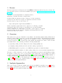
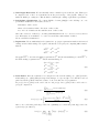
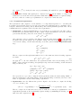
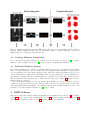
Knee Segmentation and Registration Toolkit (KSRT)
Automatic Cartilage Segmentation and Cartilage Thickness Analysis
Software Release: 1.0
https://bitbucket.org/marcniethammer/ksrt/wiki/Home
Junpyo Hong
Liang Shan
Marc Niethammer
January 22, 2015
Contents
1 License
2
2 Overview
2
3 Analysis Approaches
3.1 Cartilage Segmentation . . . . . . . . . . . . . .
3.1.1 Preprocessing . . . . . . . . . . . . . . . .
3.1.2 Multi-Atlas-Based Bone Segmentation . .
3.1.3 Multi-Atlas-Based Cartilage Segmentation
3.1.4 Longitudinal Segmentation . . . . . . . .
3.2 Cartilage Thickness Computation . . . . . . . . .
3.3 Statistical Thickness Analysis . . . . . . . . . . .
.
.
.
.
.
.
.
.
.
.
.
.
.
.
.
.
.
.
.
.
.
.
.
.
.
.
.
.
.
.
.
.
.
.
.
.
.
.
.
.
.
.
.
.
.
.
.
.
.
.
.
.
.
.
.
.
.
.
.
.
.
.
.
.
.
.
.
.
.
.
.
.
.
.
.
.
.
.
.
.
.
.
.
.
.
.
.
.
.
.
.
.
.
.
.
.
.
.
.
.
.
.
.
.
.
.
.
.
.
.
.
.
.
.
.
.
.
.
.
.
.
.
.
.
.
.
.
.
.
.
.
.
.
.
.
.
.
.
.
.
.
.
.
.
.
.
.
.
.
.
.
.
.
.
.
.
.
.
.
.
.
.
.
.
.
.
.
.
.
.
.
.
.
.
.
2
3
4
4
5
7
8
8
4 KSRT Software
4.1 Overview of the Software Pipeline
4.1.1 Overview of Scripts . . . .
4.1.2 Prerequisites Tasks . . . . .
4.2 Image Data Format . . . . . . . . .
4.3 Building the Software . . . . . . .
4.3.1 Dependencies . . . . . . . .
4.3.2 Utility Applications . . . .
4.3.3 Build Instruction . . . . . .
4.4 Supported Platform . . . . . . . .
.
.
.
.
.
.
.
.
.
.
.
.
.
.
.
.
.
.
.
.
.
.
.
.
.
.
.
.
.
.
.
.
.
.
.
.
.
.
.
.
.
.
.
.
.
.
.
.
.
.
.
.
.
.
.
.
.
.
.
.
.
.
.
.
.
.
.
.
.
.
.
.
.
.
.
.
.
.
.
.
.
.
.
.
.
.
.
.
.
.
.
.
.
.
.
.
.
.
.
.
.
.
.
.
.
.
.
.
.
.
.
.
.
.
.
.
.
.
.
.
.
.
.
.
.
.
.
.
.
.
.
.
.
.
.
.
.
.
.
.
.
.
.
.
.
.
.
.
.
.
.
.
.
.
.
.
.
.
.
.
.
.
.
.
.
.
.
.
.
.
.
.
.
.
.
.
.
.
.
.
.
.
.
.
.
.
.
.
.
.
.
.
.
.
.
.
.
.
.
.
.
.
.
.
.
.
.
.
.
.
.
.
.
.
.
.
.
.
.
.
.
.
.
.
.
.
.
.
.
.
.
.
.
.
.
.
.
.
.
.
.
.
.
.
.
.
.
.
.
.
.
.
8
9
9
9
10
10
11
11
11
12
5 Tutorial: Pfizer Longitudinal Study Dataset
5.1 PLS Dataset . . . . . . . . . . . . . . . . . .
5.2 Running the Software Pipeline . . . . . . . .
5.2.1 Preprocessing . . . . . . . . . . . . . .
5.2.2 Training Classifiers . . . . . . . . . . .
5.2.3 Automatic Cartilage Segmentation . .
5.3 Longitudinal Segmentation . . . . . . . . . .
5.4 Cartilage Thickness Computation . . . . . . .
5.5 Statistical Analysis on the Thickness . . . . .
.
.
.
.
.
.
.
.
.
.
.
.
.
.
.
.
.
.
.
.
.
.
.
.
.
.
.
.
.
.
.
.
.
.
.
.
.
.
.
.
.
.
.
.
.
.
.
.
.
.
.
.
.
.
.
.
.
.
.
.
.
.
.
.
.
.
.
.
.
.
.
.
.
.
.
.
.
.
.
.
.
.
.
.
.
.
.
.
.
.
.
.
.
.
.
.
.
.
.
.
.
.
.
.
.
.
.
.
.
.
.
.
.
.
.
.
.
.
.
.
.
.
.
.
.
.
.
.
.
.
.
.
.
.
.
.
.
.
.
.
.
.
.
.
.
.
.
.
.
.
.
.
.
.
.
.
.
.
.
.
.
.
.
.
.
.
.
.
.
.
.
.
.
.
.
.
.
.
.
.
.
.
.
.
.
.
.
.
.
.
.
.
.
.
.
.
.
.
.
.
.
.
.
.
.
.
.
.
.
.
.
.
.
.
.
.
12
12
14
14
15
16
30
30
31
.
.
.
.
.
.
.
.
.
.
.
.
.
.
.
.
.
.
.
.
.
.
.
.
.
.
.
.
.
.
.
.
.
.
.
.
.
.
.
.
.
.
.
.
.
1
1
License
The Knee Segmentation and Registration Toolkit (KSRT) is distributed under the Apache 2.0 license. For
more information, please see the license file within the git repository [email protected]:marcniethammer/
ksrt.git.
Copyright (c) 2014 Department of Computer Science,
University of North Carolina at Chapel Hill
Licensed under the Apache License, Version 2.0 (the "License");
you may not use this file except in compliance with the License.
You may obtain a copy of the License at
http://www.apache.org/licenses/LICENSE-2.0
Unless required by applicable law or agreed to in writing, software
distributed under the License is distributed on an "AS IS" BASIS,
WITHOUT WARRANTIES OR CONDITIONS OF ANY KIND, either express or implied.
See the License for the specific language governing permissions and
limitations under the License.
2
Overview
This software is an open source distribution of algorithms to automatically quantify cartilage thickness from
magnetic resonance (MR) images and to perform related statistical analyses. The implemented algorithms
are in detail described in [3]. This document serves as a high-level overview, contains an installation guide,
as well as a tutorial to guide a user through a data analysis. In particular, the software described in this
user manual allows to automatically performs the following analysis tasks:
1) Segmenting cartilage from knee Magnetic Resonance Imaging (MRI) data.
2) Computing cartilage thickness from the automatic cartilage segmentations.
3) Establishing spatial correspondence across MRI data appropriate for statistical analysis.
4) Performing statistical analysis of localized cartilage changes for cross-sectional and longitudinal data.
The purpose of this document is to provide background information necessary for understanding and using
the software so that it can be used on other datasets. The software has so far successfully been applied
to analyze data from the Pfizer Longitudinal Study [2, 3] as well as from the MICCAI SKI10 challenge on
cartilage segmentation [2]. A summary of the obtained results can be found in [2].
Section 3 gives an overview of the analysis approaches used. For a more detailed explanation please refer
to [3]. Section 4 illustrates how to build the software. Section 5 presents a tutorial on how to use the software
to analyze the Pfizer Longitudinal Dataset.
3
Analysis Approaches
This section describes briefly the analysis approaches used in KSRT. Specifically, Section 3.1 describes
how cartilage segmentation is performed, Section 3.2 discusses the cartilage thickness computations, and
Section 3.3 describes the statistical analysis approach.
2
Figure 1: Flowchart of overall cartilage segmentation pipeline
3.1
Cartilage Segmentation
KSRT uses a multi-atlas-based segmentation approach [3] with non-local patch-based label fusion. Figure 1
shows a flow-chart of the overall analysis pipeline, which consists of the following steps. First, both the femur
bone and the tibia bone are automatically segmented using a multi-atlas strategy. These bone segmentations
are used for an initial rough image alignment and to automatically extract a smaller region around the knee
joint within which a refined registration and the segmentation of cartilage is performed. Focusing on this
smaller region significantly reduces the computational cost of the approach. The cartilage segmentation
itself is based on a spatial prior obtained from multi-atlas registration of labeled joint regions and a datalikelihood terms obtained through local feature-based probabilistic classification. Both the spatial prior and
the data-likelihoods are used within a three-label convex segmentation formulation to obtain the segmentation
labels for femoral and tibial cartilage as well as background. The three-label segmentation makes use of an
anisotropic spatial regularization term to simultaneously suppress noise while respecting the thin cartilage
structures.
In the context of atlas-based segmentation, an atlas [1] is defined as the pair of an original structural
image and the corresponding segmentation. The segmentation in the atlas pair is assumed to be obtained
for example by manual segmentation by a domain expert.
3
Suppose we have N atlases, then in each atlas Ai (i = 1, 2, ..., N ), we have
• A Structural Image, Ii
• A Manual Segmentation of the Femur bone, SiF B
• A Manual Segmentation of the Tibia bone, SiT B
• A Manual Segmentation of the Femoral cartilage, SiF C
• A Manual Segmentation of the Tibial cartilage, SiT C
The remainder of this section provides brief descriptions for each stage of the segmentation pipeline.
Section 3.1.1 gives an overview of the preprocessing required for datasets prior to cartilage segmentation and
statistical analysis. Section 3.1.2 explains the multi-atlas-based automatic segmentation of the femur and
the tibia. Section 3.1.3 explains how femoral and tibial cartilage are segmented using a multi-atlas segmentation strategy guided by the segmentations of femor and tibia. Finally, Section 3.1.4 shows how cartilage
segmentations can be refined for longitudinal data (as available for example from the Pfizer Longitudinal
Study or the data of the Osteoarthritis Initative) by enforcing temporal regularity.
3.1.1
Preprocessing
Before we can use the data for analysis some preprocessing needs to be performed. We first remove artifacts
in images caused by the nonhomogeneity in magnetic fields. Then we rescale image intensities so that values
range from 0 to 100. We perform edge preserving smoothing to further remove noise in the images. Finally
we downsample the images by a factor of 4 for the first 2 dimensions to make image registration more
efficient while not losing too much information. Note that this only affects the registration, segmentation is
still performed at the full image resolution.
3.1.2
Multi-Atlas-Based Bone Segmentation
After the data is pre-processed appropriately for the analysis, we automatically segment knee bones from
the images using a multi-atlas strategy. The labeling cost c of each voxel location x in the query image for
each label l in F B, BG, T B (”F B”, ”BG”, and ”T B” denotes the femur bone, the background, and the
tibia bone respectively) are defined by log-likelihoods :
p(I(x)|l) · P (l)
c(x, l) = − log (P (l|I(x))) = − log
∝ − log (p(I(x)|l) · P (l))
(1)
p(I(x))
We first segment femur bone and tibia bone from the query image by performing the following steps:
1) Registration: We compute spatial transformation to register each of the atlases to the query image.
We first compute affine transformation based on structural images of each atlases and the query such
that
Tiaf f ine : Ii → Iq .
(2)
Then we apply Tiaf f ine computed from (2) to Ii , SiF B , and SiT B (i = 1, 2, ..., N ).
Tiaf f ine ◦ Ii
Tiaf f ine ◦ SiF B
(3)
Tiaf f ine ◦ SiT B
This is followed by a B-Spline transformation such that
Tibspline : (Tiaf f ine ◦ Ii ) → Iq
4
(4)
Just as for the affine transformation, we apply the transformation computed in (4) to Tiaf f ine ◦ Ii ,
Tiaf f ine ◦ SiF B , and Tiaf f ine ◦ SiT B
Tibspline ◦ Tiaf f ine ◦ Ii
Tibspline ◦ Tiaf f ine ◦ SiF B
Tibspline
◦
Tiaf f ine
◦
(5)
SiT B
2) Label Fusion: We propagate the registered segmentation masks, i.e., Tibspline ◦ Tiaf f ine ◦ SiF B and
Tibspline ◦ Tiaf f ine ◦ SiT B to form the spatial prior of the femur bone and the tibia bone, i.e., p(F B) and
p(T B), for the query image Iq :
p(F B) =
N
1 X bspline
◦ Tiaf f ine ◦ SiF B
Ti
N i=1
N
1 X bspline
p(T B) =
Ti
◦ Tiaf f ine ◦ SiT B
N i=1
(6)
where F B and T B respectively denote the femur bone and the tibia bone.
Recall from 3.1.1 that we have downsampled the image to make registration efficient while not losing
too much information. After summation and division in (6), we upsample p(F B) and p(T B) back to
the original dimension.
3) Segmentation: Finally, we segment the femur bone and the tibia bone from the query by minimizing
the labeling cost of each voxel location for the femur bone and the tibia bone. Recall from (1) that
this cost is expressed in terms of posterior probability:
c(x, F B) = − log (p (F B|I (x))) ∝ − log (p(I(x)|F B) · p(F B))
c(x, T B) = − log (p (T B|I (x))) ∝ − log (p(I(x)|T B) · p(T B))
(7)
where x denotes each voxel location in the image, and I(x) denotes intensity value at x.
The likelihood of the femur bone and the tibia bone, i.e., p(I(x)|F B) and p(I(x)|T B), are computed
as the following.
p(I(x)|F B) = p(I(x)|T B) = exp(−βI(x))
(8)
where β is set to 0.02 and the intensity values I(x) range from 0 to 100 as a result of the preprocessing
described in 3.1.1
We use the three-label segmentation described in [3] to segment the femur bone and the tibia bone by
minimizing labeling costs (7).
3.1.3
Multi-Atlas-Based Cartilage Segmentation
After segmenting the knee bones from the query (denoted by S F B and S T B ), we can use these segmentation
masks to guide cartilage segmentation. The labeling cost for the femoral cartilage and the tibial cartilage
is expressed in terms of posterior probabilities: with priors computed from multi-atlas-based registration
followed by non-local patch-based label fusion and likelihoods computed from probabilistic classification (we
use a Support Vector Machine (SVM)). The labeling cost c of each voxel x for each label l in F C, BG, T C
(”F C”, ”BG”, ”T C” respectively denote the femoral cartilage, the background, and the tibial cartilage) is,
p (f (x) |l) · p (l)
c(x, l) = − log (P (l|f (x))) = − log
∝ − log (p (f (x) |l) · p (l))
(9)
p (f (x))
We perform the following steps to automatically segment both cartilages from the query.
5
1) Joint Region Extraction: We automatically extract a smaller region around the joint. This region
is computed based on the bone segmentation from the previous stage of the pipeline. This process
makes the further processing more efficient while not affecting the cartilage segmentation performance.
2) Probabilistic Classification: We compute likelihood terms p(f (x)|l) for the labeling cost c via
probabilistic classification. For features, we used:
• intensities on three scales
• first-order derivatives in three directions on three scales
• second-order derivatives in the axial directions on three scales
where three scales are obtained by convolving with Gaussian kernels of σ = 0.3 mm, 0.6 mm, and 1.0
mm. All features are normalized to be centered at 0 and have unit standard deviation.
We use an SVM for classification.
3) Registration: We use multi-atlas-based registration to propagate segmentation masks for the femoral
cartilage and the tibial cartilage. We register each atlas Ai to the query via computing affine transformations:
af f ine
Ti,F
: SiF B → S F B
C
(10)
af f ine
Ti,T
: SiT B → S T B
C
af f ine
af f ine
We apply Ti,F
to the femoral cartilage segmentation SiF C and the structural image Ii , and Ti,T
C
C to
TC
the tibial cartilage segmentation Si and the structural image Ii .
af f ine
S̃iF C = Ti,F
◦ SiF C
C
af f ine
I˜iF C = Ti,F
◦ Ii
C
(11)
af f ine
S̃iT C = Ti,T
◦ SiT C
C
af f ine
I˜iT C = Ti,T
◦ Ii
C
4) Label Fusion: After the registration, we form priors for the femoral cartilage (i.e., p(F C)) and the
tibial cartilage (i.e., p(T C)) using the warped label images, i.e., S̃iF C and S̃iT C . Note that the non-local
patch based strategy in label fusion is robust to local errors introduced by registration.
Let pF C (x) denote p(F C) at the voxel location x and pT C (x) denote p(T C) at the voxel location x.
pF C (x) is computed as:
N P
P
FC
(x, y)S̃iF C (y)
y∈N (x) w
i=1
FC
,
(12)
p (x) =
N P
P
F C (x, y)
w
y∈N (x)
i=1

2 
I(x0 ) − I˜iF C (y 0 ) 
,
hF C (x)
P

wF C (x, y) = exp 
x0 ∈P(x)y 0 ∈P(y)
(13)
where x0 is a voxel in the patch P(x) centered at x (similarly y 0 a voxel in the patch P(y) centered at
y) and hF C (x) is defined by
hF C (x) = min
X 1≤i≤N 0
y∈N (x) x ∈P(x)
y 0 ∈P(y)
6
I(x0 ) − I˜iF C (y 0 )
2
+
(14)
We compute pT C (x) exactly the same way by substituting F C with T C in equations: (12), (13),
and (14).
5) Segmentation: Finally with spatial priors computed from (12) and the likelihood computed via
classification, we use the three-label segmentation with anisotropic regularization to segment cartilage.
In order to make use of anisotropic regularization, we compute the normal directions.
3.1.4
Longitudinal Segmentation
The segmentation result computed so far is assumed to be temporally independent. I.e., each timepoint
is segmented independently. However, if we know the dataset is longitudinal, then we can further enforce
temporal consistencies across image data at different time points. Our longitudinal segmentation also follows
a similar framework: registration followed by three-label segmentation.
1. Registration: To align longitudinal images of a given subject, we register all of the time points to
the first time-point (baseline image). We first compute a rigid transformation between the t−th time
point and the first time point based on the femur bone segmentation.
RtF B : StF B → S0F B
(15)
where subscript t denotes t−th time point. Then we apply the transformations (15) to: the segmentation mask of the femoral cartilage, the local likelihood map of the femoral cartilage, spatial prior map
of the femoral cartilage, and the structural image around the joint from Joint Region Extraction
stage.
RtF B ◦ StF C
RtF B ◦ pt (f (x)|F C)
RtF B ◦ pt (F C)
(16)
RtF B ◦ Itjoint
Then we compute another rigid transformation based on the transformed femoral cartilage segmentation mask.
RtF C : RtF B ◦ StF C → S0F C
(17)
We apply RtF C to all of the transformed: the segmentation mask of the femoral cartilage, the local
likelihood map of the femoral cartilage, the spatial prior map of the femoral cartilage, and the structural
image around the joint.
S̃tF C = RtF C ◦ RtF B ◦ StF C
p̃t (f (x)|F C) = RtF C ◦ RtF B ◦ pt (f (x)|F C)
p̃t (F C) = RtF C ◦ RtF B ◦ pt (F C)
I˜tjoint = RtF C ◦ RtF B ◦ Itjoint
(18)
We repeat the above procedure to align the tibial segmentation mask, the tibial cartilage likelihood
map, the spatial prior for the tibial cartilage, and the structural image around the joint based on the
tibia bone segmentation and the tibial cartilage segmentation.
2. Segmentation: Once the different time point are aligned to the baseline, we compute the labeling
cost c for t−th time point,
p̃t (f (x) |l) · p̃t (l)
∝ − log (p̃t (f (x) |l) · p̃t (l))
(19)
c(x, l, t) = − log (pt (l|f (x))) = − log
p̃t (f (x))
Then we compute the normal directions because we make use of anisotropic regularization for the
longitudinal segmentation. We longitudinally segment cartilages by minimizing the labeling cost (19)
with each terms computed from (18).
7
Figure 2: Thickness Computation pipeline. Extract the joint region and automatically segment cartilages.
Compute cartilage thickness. Register all of the 3D thickness maps to a common atlas space. Project 3D
thickness maps onto a 2D plane along axial direction.
3.2
Cartilage Thickness Computation
Once both femoral and tibial cartilages are segmented we use the method described in [4] to compute
thickness of those cartilages. Please refer [4] for more details on computing tissue thickness.
3.3
Statistical Thickness Analysis
Once cartilage thicknesses are computed we establish spatial correspondence of the thicknesses by mapping
them to a common atlas space. We use an affine followed by B-Spline transform which are computed based
on bone segmentations for each cartilage thickness volume. Then these transformed thicknesses are projected
down to an axial slice by taking the median thickness value along the axial direction (where thicknesses are
approximately constant). Then these thickness maps are comparable across time-points and subjects. Note
that all segmentations and thicknesses are computed in native image space. Figure 3.3 illustrates how the
thickness maps are computed.
Once the 2D thickness maps are created we first fit a linear mixture model to model differences between
normal control subjects and OA subjects. Then we cluster OA subjects such that subjects in the same
cluster have similar patterns in thinning of the cartilages. Then we fit another linear mixture models to each
OA cluster for a refined statistical analysis. See [3] for more details.
4
KSRT Software
This section describes the software available implementing the algorithms described in Section 3. Specifically,
Section 4.1 gives an overview of the software pipeline. Section 4.2 discusses the image format used. Section 4.3
discusses how to build the software. Section 4.4 discusses the supported platforms.
8
4.1
Overview of the Software Pipeline
This software package contains several components for automatic segmentation of cartilage. In what follows,
we will give an overview of all the stages of the analysis pipeline. The source code distribution contains the
following directories:
• src: This directory contains C++ implementation of the algorithm.
• lib: This directory contains various applications used.
• scripts: This directory contains scripts to run the segmentation on a compute cluster.
• matlab: This directory contains scripts written in MATLAB to perform statistical analysis on cartilage
thickness.
4.1.1
Overview of Scripts
In the source code distribution we provide scripts to submit jobs on clusters using the qsub command to
automatically segment cartilage from query images.
Under the scripts directory, you will find the following job submission scripts:
• submit_Preprocess: This script performs preprocessing on the dataset as described in 3.1.1.
• submit_TrainSVM: This script trains SVM classifiers using the libSVM implementation. Three SVM
classifiers for the femoral cartilage, the background, and the tibial cartilage are trained. The trained
classifiers are saved to be used during the cartilage segmentation.
• submit_CartSeg_indp: This script is the main script that automatically segments femoral and tibial
cartilage from query images as described in 3.1. In order to run this script successfully, some prerequisite
tasks need to be performed prior to executing the script. Please refer to Section 4.1.2 for the details
on these tasks.
• submit_temporal_align: This script enforces temporal consistencies across segmentation results of
different time points of a single subject. In order to run this script successfully the dataset needs to
be longitudinal and also needs to be organized in a specific way as described later in this document.
• submit_CartSeg_long: This script refines segmentation results via establishing spatial correspondence
across different time points.
4.1.2
Prerequisites Tasks
To run the pipeline using the provided scripts the following path variables need to be defined. If you are using
bash, then follow the instructions below to define path variables in your .bashrc so that scripts running
the pipeline can access the appropriate paths. In addition, you need to create two text files to denote
query images and atlas images in the dataset so that the aforementioned scripts can access and process data
appropriately.
• Path Variables
– ksrt Application Directory: You have to define ksrt Application directory as ksrtAppDIR in
your system setting file. If you are using bash, then put the following in your .bashrc.
AppDIR=/home/username/ksrt/build/Application
export AppDIR
– ksrt Library Directory: If you choose to use the provided scripts to run the pipeline, then put
the following in your .bashrc.
9
LibDIR=/home/username/ksrt/lib
export LibDIR
– Dataset Directory: You have to define DataDIR to be the path to your dataset. Please put the
following in your .bashrc.
DataDIR=/home/username/your_path_to_data
export DataDIR
– Slicer Directory: If you choose to use the provided scripts to run the pipeline on a compute
cluster, some of applications that are part of Slicer3 are needed. Please put the following lines in
your .bashrc.
SlicerDIR=/home/username/your_path_to_Slicer
export SlicerDIR
• Text files: Below are the text files needed. Place these two text files where the dataset is. That is
the directory pointed by $DataDIR defined in .bashrc.
– list.txt: This text file contains a list of all query images to be segmented. This text file needs
to list relative paths to the query images from $DataDIR. For example, list.txt used later in 5
looks like the following.
site1001
site1001
site1001
site1001
site1001
site1001
.....
10011003
10011003
10011003
10011003
10011003
10011004
0
3
6
12
24
0
With each row corresponding to a single query image. There are three columns per row. The first
column denotes which site directory the query image resides in. The second column denotes the
subject id of the query image. Lastly, the third column denotes the time point of the query image
(in month).
– list_atlas.txt: This text file contains a list of all atlas images. The format is exactly the same
as list.txt.
4.2
Image Data Format
We use the Nearly Raw Raster Data (NRRD) format throughout the analysis. See teem.sourceforge.net/
nrrd for a detailed description of this format. This data format is supported by ITK (www.itk.org). AS
our analysis software uses ITK to read and write images other ITK supported file-formats could in principle
also easily be supported in future releases of the software. For now please convert all your data to NRRD
format before running this software. This conversion could for example be done using Slicer or using a
simple ITK script.
4.3
Building the Software
KSRT depends on a number of different open-source packages which are freely available online. CMake is
used to configure the build and is available from http://www.cmake.org. Earlier versions of CMake may
not be supported so we recommend downloading CMake at least higher than version 2.6.
10
4.3.1
Dependencies
To build the software, you will need the following packages. If you have already built Slicer-3, then you
only need to build the Approximate Nearest Neighbor library and the ImageMath package.
• InsightToolkit 3.20 (ITK3) is required for all of applications in KSRT package. Both ITK3 and
ITK4 are available to download at http://www.itk.org.
• Slicer-3 is also required to build KSRT successfully. It is available to download from http://www.
slicer.org/slicerWiki/index.php/Slicer3:Downloads.
• ann 1.1.2 is required to build KSRT. This is an open-source library for approximate nearest neighbor
search and is available to download at http://www.cs.umd.edu/~mount/ANN/. This is provided as a
part of the software distribution.
4.3.2
Utility Applications
In addition, the software uses several applications. These applications are not required to build KSRT,
but these are required to run the pipeline using the provided scripts successfully. These applications are
included as part of the source code distribution. Below are the list of the applications used along with short
descriptions.
• ImageMath is an open-source C++ library for mathematical operations on images. It is available to
download at http://www.nitrc.org/projects/niral_utilities/.
• ExtractLargestConnectedComponentFromBinaryImage is used to segment the largest connected component from a binary image. This is used to segment out bones and cartilages after the labeling cost of each object is computed. This application can be found under /path_to_ksrt_source/lib/ExtractLargestC
A detailed description of the application is available at http://www.itk.org/Wiki/ITK/Examples/
ImageSegmentation/ExtractLargestConnectedComponentFromBinaryImage.
• libsvm-3.17 is a C++ implementation of Support Vector Machine libraries. This is needed if you wish
to use SVM to compute likelihoods which in turn are used to compute labeling costs. It is available to
download at http://www.csie.ntu.edu.tw/~cjlin/libsvm/.
4.3.3
Build Instruction
CMake is used to configure the build and generate Makefiles or Visual Studio Solution files. After successfully configuring, the software can be built using the native compiler. For information on using CMake,
please refer to http://www.cmake.org.
The following section provides step-by-step instruction on how to build dependent packages.
• Slicer3 Please refer for build instructions on building Slicer3 http://www.slicer.org/slicerWiki/
index.php/Slicer3:Build_Instructions. When finished building Slicer3, ITK3 will also be downloaded and installed.
Once all of dependent applications are built, then please follow the steps below to build KSRT.
1. Clone the git source code distribution at [email protected]:marcniethammer/ksrt.git by executing
g i t c l o n e g i t @ b i t b u c k e t . o r g : marcniethammer / k s r t . g i t
2. Create a separate directory for your build files and executables. For example, if you cloned the source
code distribution in /home/username/ksrt, then you may create a separate directory named
/home/username/ksrt-build.
11
3. Change into the build directory created in the previous step. Then runccmake ../ksrt in the terminal
to configure KSRT.
4. Below are the list of path variables needed to configure KSRT successfully.
• ANN LIB is a path to actual library file which is located at ksrt/lib/ann_1.1.2/lib/libANN.a
directory of the source code distribution.
• ANN PATH is path to include directory of ann 1.1.2 package.
This directory is at ksrt/lib/ann_1.1.2/include
• Slicer3 DIR is a path build directory of Slicer3.
• GenerateCLP DIR is a path to a package that comes with Slicer3. This package should be
located at under the build directory of Slicer3 that looks like the following.
your_path_to_slicer3/Slicer3-build/Libs/SlicerExecutionModel/GenerateCLP
• ITK3 DIR is also installed along with Slicer3. This should be set to something like the following.
your_path_to_slicer3/Slicer3-lib/Insight-build
Once these path variables are set, then let CMake configure again and again until CMake can
configure the build without any errors.
5. Once Configured, you can generate the build, i.e., Makefile for KSRT.
6. Use make command to build KSRT.
4.4
Supported Platform
We have built and tested the software package under Unix-based system (e.g. Linux and MacOSx). We
recommend running the system on a cpmpute cluster as some parts of the pipeline are computationally
demanding, but can be computed in parallel on a cluster.
5
Tutorial: Pfizer Longitudinal Study Dataset
We will illustrate how to segment cartilage using the Longitudinal Multi-Atlas Approach based on the Pfizer
Longitudinal Dataset. The software can be run in a similar way on the SKI10 and the OASIS datasets.
This tutorial provides step-by-step instructions to run the software for analyzing longitudinal changes in
cartilage thickness on subjects. In this example, we will use the Multi-Atlas based cartilage segmentation
with longitudinal constraints.
5.1
PLS Dataset
The Pfizer Longitudinal Study (PLS) dataset contains 706 T1-weighted (3D SPGR) images for 155 subjects,
imaged at baseline, 3, 6, 12, and 24 months at a resolution of 1.00 × 0.31 × 0.31mm3 . Some subjects have
missing scans. The kellgren-Lawrence grades (KLG) were determined for all subjects from the baseline scans,
classifying 82 as normal control subjects (KLG0), 40 as KLG2, and 33 as KLG3.
For the distribution of this dataset that was available to us the top level directory of the dataset consisted
of seven directories, each representing different sites where subjects received longitudinal MRI assessments
of their knees.
site1001
site1002
site1003
site1004
12
site1005
site1006
site1007
Inside each of the aforementioned site directories, MRI data is grouped by directories named after unique
subject ids that contain longitudinal knee MRI measurements of the subject with that id. These folders
contain varying number of subjects. For example, under the directory site1001, there are 29 folders, each
storing longitudinal knee MRI data of a subject imaged at this site.
10011003,
10011004,
10011005,
.....
10011055
Lastly inside of each of the subject folder is a longitudinal collection of knee MRI data that are stored
separately for different time points of the measurement. The name of folders is the number of the months
after the initial scan; therefore, the first MRI measurement (baseline MRI data) is under 0. For example,
under 10011003, there are five folders named
0,
3,
6,
12,
24.
The aforementioned folders contain the following files:
• Structural MR image: cor_t1.nhdr and cor_t1.raw.gz
• Manual segmentation of the femoral cartilage: fem.nhdr and fem.raw.gz
• Manual segmentation of the tibial cartilage: tib.nhdr and tib.raw.gz
Both manual segmentation of the femoral cartilage and of the tibial cartilage (drawn by a domain expert,
Dr. Felix Eckstein) are available for all images. However these manual segmentations are only used for
evaluating the quality of automatic cartilage segmentation; therefore these segmentations are not strictly
needed to run the software.
Recall from 3.1, we make use of the knee bone segmentations to guide cartilage segmentations. Expert
segmentation on the femur bone and on the tibia bone are only available for us for the baseline images of 18
subjects. These 18 baseline images serve as atlases A which are necessary to run our software pipeline. When
the aforementioned folder is one of these 18 baseline image (atlas image) folders, then the folder contains
the following files:
• Structural MR image: cor_t1.nhdr and cor_t1.raw.gz
• Manual segmentation of the femur bone: femur.nhdr and femur.raw.gz
• Manual segmentation of the femoral cartilage: fem.nhdr and fem.raw.gz
• Manual segmentation of the tibia bone: tibia.nhdr and tibia.raw.gz
• Manual segmentation of the tibial cartilage: tib.nhdr and tib.raw.gz
There are a total of 706 images in the PLS dataset.
13
5.2
Running the Software Pipeline
In this section we describe the expected output after running the provided scripts. Recall that prerequisite
tasks described in 4.1.2 need to be done prior to running the scripts.
5.2.1
Preprocessing
As previously discussed, the first step is to process the data appropriately for analysis. By executing
preprocess.sh we perform the preprocessing on the entire dataset as described in 3.1.1. Type the following
command to run preprocessing scripts on the dataset.
qsub s u b m i t P r e p r o c e s s
We store all of the intermediate results of the preprocessing. Below are the list of files that are saved as
the intermediate results of the preprocessing.
• cor_t1_correct: Bias field caused by magnetic non-homogeneity is corrected from the original image
cor_t1.
• cor_t1_correct_scale: Intensity values of cor_t1_correct are rescaled so that values are between
0 and 100
• cor_t1_correct_scale_smooth: The result of the previous step, i.e., cor_t1_correct_scale, are
smoothed while preserving edges in the image.
• cor_t1_correct_scale_smooth_small: The smoothed image, i.e., cor_t1_correct_scale_smooth,
is downsampled to be used during registration.
Figure 3 shows the result of the preprocessing on an image taken at baseline for subject 10011003.
14
(a)
(b)
(c)
(d)
Figure 3: Result of preprocessing of a subject baseline image: (a) bias-field corrected image, (b) intensityscaled image, (c) smoothed image, (d) downsampled image.
5.2.2
Training Classifiers
The next step is to train SVM classifiers to be used during cartilage segmentation to provide likelihood terms
for the labeling cost in (9). We train SVM classifiers to perform probabilistic classification of the femoral
cartilage, the background, and the tibial cartilage. The classifier outputs probabilities of each voxels in the
image belonging to the femoral cartilage, the background, and the tibial cartilage. The classifier is trained
using features described in 3.1.3 extracted from the atlas images.
Type the following command in the terminal to train the SVM classifier.
qsub submit TrainSVM
The script first creates a folder named SVM at the dataset directory to save trained classifiers and extracted
features. The path to this folder looks something like the following.
$DataDIR/SVM
Once the directory is created (or already exists) the following files are saved in the folder after the execution
of the script.
• cor_t1_correct_scale_30000: Intensity values of the atlas images are rescaled to range from 0 to
30000 prior to feature extraction. Recall that after the preprocessing intensity values of the image
15
range from 0 to 100.
• trainLabel.nhdr: Label image extracted to be used in the training
• train_1: Features extracted for the femoral cartilage.
• train_2: Features extracted for the background.
• train_3: Features extracted for the tibial cartilage.
• train_1_small: subset of train_1 to be used during training
• train_2_small: subset of train_2 to be used during training
• train_3_small: subset of train_3 to be used during training
• train_small: Concatenation of train_1_small, train_2_small, and train_3_small
• train_balance.model: trained SVM classifier.
5.2.3
Automatic Cartilage Segmentation
Once the classifiers are trained we are now ready to process the query images. Please type the following
command in the terminal.
qsub s u b m i t C a r t S e g i n d p
In this section we provide what to expect as an output for each stage in the script along with visualization
of intermediate results.
Bone Registration
We register all of atlases to a given query image via computing a series of spatial transformations.
During execution, files are saved to an output directory of the form
$DataDIR/$SITEID Q/$ID Q/$VISIT Q/ m o v e d a t l a s
where $SITEID_Q is one of the site directories described in 5.1, $ID_Q is one of the subject id directories
under the SITEID_Q, and $VISIT_Q is one of the measurement time points of that subject denoted by $ID_Q.
If the output directory does not exist, the script creates the output directory first. Once the output directory
is created (or already exists), you should find the following files in the output directory.
• affine transform file: affine_$ID_A.tfm
• B-Spline transform file: bspline_$ID_A.tfm
• transformed structural image: moved_$ID_A.nhdr and moved_$ID_A.raw.gz
• transformed femur bone segmentation: moved_femur_$ID_A and moved_femur_$ID_A.raw.gz
• transformed tibia bone segmentation: moved_tibia_$ID_A and moved_tibia_$ID_A.raw.gz
$ID_A denotes different IDs of atlas subjects.
16
Bone Label Fusion
After the registration, we fuse all of the moved segmentations of the atlases to form the prior probability
of a voxel belonging to the femur bone. We simply take an arithmetic mean of all of the transformed
segmentation masks to form the prior probability map for the femur bone p(F emur) and the tibia bone
p(T ibia) respectively. Two images named pFemur and pTibia are saved after the label fusion. Figure 4
illustrates what these prior probability maps look like.
(a)
(b)
Figure 4: Spatial prior probability map for the femur bone (left, a) and the tibia bone (right, b).
Bone Segmentation
We compute bone likelihoods for each voxel, which are saved as pBone. Given bone likelihoods and priors we
compute the labeling cost map for the femur bone, the background, and the tibia bone; these are saved as
cost_femur, cost_bkgrd, and cost_tibia respectively. These labeling cost maps are used within a threelabel segmentation method to segment the femur bone and the tibia bone. Figure 5 shows visualizations of
these costs.
17
Figure 5: Labeling costs for the femur bone (top), the background (middle), and the tibia (bottom).
18
There is a regularization parameter to choose in segmentation method (see [3] for details); this optimization; we set this parameter to 0.5. Figure 6 shows the final bone segmentations.
Figure 6: Final bone segmentations.
Extract Joint Region
We automatically extract a smaller region (from this point on, we refer this region as joint region) from
the original images to make the further processing more efficient. These regions are automatically extracted
using the bone segmentation masks from the structural image, the femur bone segmentation mask, and the
tibia bone segmentation mask.
In addition, we create another structural image which is a rescaled version of the structural image of the
joint region. The intensity values are rescaled so that they range from 0 to 30000. (Recall that after the
preprocessing, intensity values range from 0 to 100.) This rescaled image is used for extracting features to
be used in classification.
During execution of the script, we store all of the smaller images extracted around the joint region to an
output directory. The output directory has the form
$DataDIR/$SITEID Q/$ID Q/$VISIT Q/ j o i n t /
where $SITEID_Q is one of the site directories described in 5.1, $ID_Q is one of the subject id directories
under the SITEID_Q, and $VISIT_Q is one of the measurement time points of that subject denoted by $ID_Q.
19
If the output directory does not exist, the script first creates the directory.
The following files are saved under the output directory after the script has finished extracting the joint
region:
• Structural image of this region: cor_t1_correct_scale
• The rescaled structural image: cor_t1_correct_scale_30000
• The femur bone segmentation mask of the region: seg_femur
• The tibia bone segmentation mask of the region: seg_tibia
Figure 7 shows the results for a sample query image.
20
Figure 7: Structural image extracted around the joint region (top), segmentation mask for the femur bone
extracted around the joint region (middle), and segmentation mask for the tibia bone extracted around the
joint region (bottom).
21
Cartilage Registration
Just as for the bone segmentation, we first register all of the atlas subjects to the query subject as a first step
of cartilage segmentation. The script first creates a folder to save the results generated during the cartilage
registration of the form
$DataDIR/$SITEID Q/$ID Q/$VISIT Q/ m o v e d c a r t a t l a s
where $SITEID_Q is one of the site directories described in 5.1, $ID_Q is one of the subject id directories
under the SITEID_Q, and $VISIT_Q is one of the measurement time points of that subject denoted by $ID_Q.
If the output directory does not exist, the script creates the output directory first. Once the output directory
is created (or already exists), the following files are saved in the output directory:
af f ine
• Ti,F
C : affine_femur_$ID_A.tfm
• I˜iF C : moved_mri_femur_$ID_A
• S̃iF C : moved_fem_$ID_A
af f ine
• Ti,T
C : affine_tibia_$ID_A.tfm
• I˜iT C : moved_mri_tibia_$ID_A
• S̃iT C : moved_tib_$ID_A
$ID_A denotes different IDs of atlas subjects.
Cartilage Tissue Classification
We perform probabilistic classification to output probabilities of a voxel belonging to three classes: the
femoral cartilage, the background, and the tibial cartilage. Recall that these probabilities will be used to
compute the likelihood terms for the labeling cost in (9).
The script first creates a folder of the following form to save results of the SVM classification:
$DataDIR/$SITEID Q/$ID Q/$VISIT Q/ j o i n t s e g e m e n t a t i o n
where $SITEID_Q is one of the site directories described in 5.1, $ID_Q is one of the subject id directories under
the SITEID_Q, and $VISIT_Q is one of the measurement time points of that subject denoted by $ID_Q. Then
features are extracted from cor_t1_correct_scale_30000 and are saved in a file named f_$ID_$VISIT in
the SVM folder ($ID and $VISIT denote subject id and the time point of the current query image respectively).
We use the trained classifier 5.2.2 to perform probabilistic classification; the output of the classification
is saved in a file named p_$ID_$VISIT under the SVM folder. The classification output is then transformed
to likelihood probability maps for the femoral cartilage and the tibial cartilage respectively; these likelihood
maps are saved under joint_segmentation.
The following files are generated as a result of classification:
• The likelihood map for the femoral cartilage: pFem_svm
• The likelihood map for the tibial cartilage: pTib_svm
Figure 8 shows the likelihood probability maps of the femoral cartilage and the tibial cartilage for one of
queries.
22
Figure 8: The classification map of the femoral cartilage (top) and of the tibial cartilage (bottom).
Cartilage Label Fusion
Once all of the atlases are registered to the query, we now fuse the registered labels of the atlases to form
spatial priors for the femoral cartilage and the tibial cartilage. We use non-local patch-based label fusion
techniques to fuse all of deformed label images.
We first upscale both deformed structural image and deformed segmentation masks by a factor of 3 to
make them approximately isotropic. Then we compute 12 for each voxel locations with patch size being set
to 2, neighborhood size set to 2, and nearest neighbor set to 5. The resulting fused labels for the femoral
cartilage and the tibial cartilages are downsampled to the original size.
After the label fusion is finished, the results are saved as images under joint_segmentation created in
the previous step. This results in:
• Non-local patch based label fusion of the femoral cartilage: fem_fusion_patch
• Non-local patch based label fusion of the tibial cartilage: tib_fusion_patch
Figure 9 shows the label fusion results for the femoral and the tibial cartilage for an example query image.
23
Figure 9: The label fusion result for the femoral cartilage (top) and the tibial cartilage (bottom).
Compute Normal Directions
The script also computes the normal directions for each dimension. These normal directions are needed
because we use anisotropic regularization during segmentation. Normal directions are saved as nx, ny, and
nz under the folder where the current query image is.
Cartilage Segmentation
Once we have computed prior probabilities from label fusion and likelihood probabilities provided by SVM,
we can now compute the labeling cost for each of the classes in terms of posterior probabilities. There
are two parameters g and a that control two regularization terms used in the optimization process. In our
example, we set g to be 1.4 and a to be 0.2. We use the normal directions computed previously because
we are segmenting the images using anisotropic regularization. For more details on these parameters, please
refer [3].
The script saves the following files under the joint_segmentation folder:
• Labeling cost of background: bkg_cost
24
• Labeling cost of the femoral cartilage: fem_cost
• Labeling cost of the tibial cartilage: tib_cost
• Segmentation mask of the femoral cartilage: seg_fem
• Segmentation mask of the tibial cartilage: seg_tib
Figure 10 shows the labeling costs for background, and the femoral and tibial cartilage respectively. Figure 11
shows the resulting segmentations for femur and tibia.
25
Figure 10: Labeling cost for the femur (top), background (middle), and tibia (bottom).
26
Figure 11: Final segmentation mask of the femoral cartilage (top) and the tibial cartilage (bottom).
Temporal Alignment
If we know the dataset is longitudinal, then we can encourage temporal consistencies among resulting cartilage
segmentation masks of different time points.
We need the following two text files for the longitudinal segmentation:
• in_aniso.txt: A text file listing input files needed for longitudinal segmentation. Each line corresponds to the femoral cartilage labeling cost, background labeling cost, the tibial cartilage labeling
cost and normal directions of different time points of a subject.
• out_aniso.txt: A text file listing output files of longitudinal segmentation. Each line corresponds to
the longitudinal segmentation of the femoral cartilage and the tibial cartilage of different time points
of a subject.
These text files are automatically generated by running the following bash script; please type the following
command in the terminal.
sh k s r t / s c r i p t / C a r t S e g L o n g P r e p r o c e s s . sh
27
Notice that this script is run as a standard bash script. Please run this script only once.
After running CartSeg_Long_Preprocess.sh, please type the following command in terminal to rigidly
align segmentation masks of different time points.
qsub s u b m i t t e m p o r a l a l i g n
The script first creates intermediate output folders for each subjects to store intermediate results of the
temporal alignment. It first creates the following folder:
$DataDIR/$SITE/$ID/ j o i n t 4 D
(Recall that $ID and $SITE denote subject id and the site id of the current query patient).
Then the script creates another folder under the joint4D folder just created to save intermediate results
of registrations.
$DataDIR/$SITE/$ID/ j o i n t 4 D / t r a n s f o r m
As noted in the previous section (i.e. section 3.1.4) we use a series of rigid registrations to temporally
align segmentation results of different time points to the baseline. The following files are the results of the
first registration which is based on bone segmentation masks. These files are saved in the transform folder.
Different time points of a subject are denoted by $VISIT.
• $VISIT_femur.tfm: Rigid transformation computed based on femur bone segmentation masks
• $VISIT_femurBased.nhdr: Rigidly transformed original structural image according to the above transformation (i.e., $VISIT_femur.tfm)
• $VISIT_femur_femurBased.nhdr: Rigidly transformed femur bone segmentation mask according to
the above transformation (i.e., $VISIT_femur.tfm)
• $VISIT_seg_fem_femurBased.nhdr: Rigidly transformed femoral cartilage segmentation mask according to the above transformation (i.e., $VISIT_femur.tfm)
• $VISIT_fem_fusion_patch_femurBased.nhdr: Rigidly transformed femoral cartilage spatial prior
map according to the above transformation (i.e., $VISIT_femur.tfm)
• $VISIT_pFem_femurBased.nhdr: Rigidly transformed femoral cartilage likelihood map according to
the above transformation (i.e., $VISIT_femur.tfm)
• $VISIT_tibia.tfm: Rigid transformation computed based on tibia bone segmentation masks
• $VISIT_tibiaBased.nhdr: Rigidly transformed original structural image according to the above transformation (i.e., $VISIT_tibia.tfm)
• $VISIT_tibia_tibiaBased.nhdr: Rigidly transformed tibia bone segmentation mask according to the
above transformation (i.e., $VISIT_tibia.tfm)
• $VISIT_seg_tib_tibiaBased.nhdr: Rigidly transformed tibial cartilage segmentation mask according
to the above transformation (i.e., $VISIT_tibia.tfm)
• $VISIT_tib_fusion_patch_tibiaBased.nhdr: Rigidly transformed tibial cartilage spatial prior map
according to the above transformation (i.e., $VISIT_tibia.tfm)
• $VISIT_pTib_tibiaBased.nhdr: Rigidly transformed tibial cartilage likelihood map according to the
above transformation (i.e., $VISIT_tibia.tfm)
28
The following files are the results of the second registration which is based on cartilage segmentation masks. The rigid transformation is computed among deformed cartilage segmentation masks (i.e.,
$VISIT_seg_fem_femurBased.nhdr and $VISIT_seg_tib_tibiaBased.nhdr). Then this transformation is
applied to deformed images, deformed segmentation masks, deformed fusion results, and deformed likelihood
maps. These files are also saved in transform folder.
• $VISIT_fem.tfm: Rigid transformation computed based on the femoral cartilage segmentation masks
• $VISIT_femBased.nhdr: Rigidly transformed original structural image according to the above transformation (i.e., $VISIT_fem.tfm)
• $VISIT_femur_femBased.nhdr: Rigidly transformed femur bone segmentation mask according to the
above transformation (i.e., $VISIT_fem.tfm)
• $VISIT_seg_fem_femBased.nhdr: Rigidly transformed femoral cartilage segmentation mask according
to the above transformation (i.e., $VISIT_fem.tfm)
• $VISIT_fem_fusion_patch_femBased.nhdr: Rigidly transformed femoral cartilage spatial prior map
according to the above transformation (i.e., $VISIT_fem.tfm)
• $VISIT_pFem_femBased.nhdr: Rigidly transformed femoral cartilage likelihood map according to the
above transformation (i.e., $VISIT_fem.tfm)
• $VISIT_tib.tfm: Rigid transformation computed based on the tibial cartilage segmentation masks
• $VISIT_tibBased.nhdr: Rigidly transformed original structural image according to the above transformation (i.e., $VISIT_tib.tfm)
• $VISIT_tibia_tibBased.nhdr: Rigidly transformed tibia bone segmentation mask according to the
above transformation (i.e., $VISIT_tib.tfm)
• $VISIT_seg_tib_tibBased.nhdr: Rigidly transformed tibial cartilage segmentation mask according
to the above transformation (i.e., $VISIT_tib.tfm)
• $VISIT_tib_fusion_patch_tibBased.nhdr: Rigidly transformed tibial cartilage spatial prior map
according to the above transformation (i.e., $VISIT_tib.tfm)
• $VISIT_pTib_tibBased.nhdr: Rigidly transformed tibial cartilage likelihood map according to the
above transformation (i.e., $VISIT_tib.tfm)
In addition to the transform folder, the script creates another folder under the joint4D folder to save
results of the longitudinal segmentation. The folder name is of the following form:
$DataDIR/$SITE/$ID/ j o i n t 4 D / s e g m e n t a t i o n
The script computes labeling cost for the femoral cartilage, background, and the tibial cartilage based on
rigidly deformed cartilage segmentation masks, fusion results, and the likelihood maps. Normal directions
are also computed because we are using anisotropic regularization for the longitudinal segmentation. The
following files are saved under the segmentation folder.
• $VISIT_fem_cost.nhdr: Labeling cost of the femoral cartilage
• $VISIT_bg_cost.nhdr: Labeling cost of the background
• $VISIT_tib_cost.nhdr: Labeling cost of the tibial cartilage
• $VISIT_nx.nhdr: Normal direction along the first dimension
• $VISIT_ny.nhdr: Normal direction along the second dimension
• $VISIT_nz.nhdr: Normal direction along the third dimension
29
5.3
Longitudinal Segmentation
Please type the following command for longitudinal three label based segmentation with anisotropic regularization.
qsub s u b m i t C a r t S e g l o n g
The following files are saved under segmentation folder.
• $VISIT_seg_fem_long.nhdr: Longitudinal segmentation masks for the femoral cartilage
• $VISIT_seg_tib_long.nhdr: Longitudinal segmentation masks for the tibial cartilage
5.4
Cartilage Thickness Computation
Please type the following command to compute tissue thickness based on the longitudinal segmentation
masks.
qsub s u b m i t T h i c k n e s s l o n g
The script will create a folder to save intermediate results of the following form:
$DataDIR/ t h i c k
Then 3D tissue thickness is computed on the results of the longitudinal segmentation. The following files
are saved under the thick folder.
• fem_$ID_$VISIT.nhdr: 3D thickness computed on longitudinal segmentation masks for the femoral
cartilage
• tib_$ID_$VISIT.nhdr: 3D thickness computed on longitudinal segmentation masks for the tibial
cartilage
Then we deform each of these 3D thickness maps to the baseline of a subject 10021014 prior to creating
2D thickness maps. This is achieved via affine transformation followed by B-Spline transformation. The
script creates another folder to save the results of these spatial transformations of the following form:
$DataDIR/ t h i c k / t r a n s f o r m
After the transform folder is created, the following files are saved.
• affine_$ID_$VISIT_femur.tfm
• bspline_$ID_$VISIT_femur.tfm
• affine_$ID_$VISIT_tibia.tfm
• bspline_$ID_$VISIT_tibia.tfm
After applying the affine followed by the B-Sspline transform, the resulting deformed 3D thickness is
saved under the folder of the following form:
$DataDIR/ t h i c k /moved
• fem_$ID_$VISIT.nhdr: Deformed 3D thickness computed on longitudinal segmentation masks for the
femoral cartilage
• tib_$ID_$VISIT.nhdr: Deformed 3D thickness computed on longitudinal segmentation masks for the
tibial cartilage
30
Finally 2D thickness maps are generated via projection of these deformed 3D thickness. The script creates
a folder to save these 2D projected thickness maps of the following form:
$DataDIR/ t h i c k / moved 2d
The following files are saved under moved_2d folder as a result of the computation:
• fem_$ID_$VISIT.nhdr: Projected 2D thickness computed on longitudinal segmentation masks for the
femoral cartilage
• tib_$ID_$VISIT.nhdr: Projected 2D thickness computed on longitudinal segmentation masks for the
tibial cartilage
5.5
Statistical Analysis on the Thickness
Once the 2D thickness maps are generated, we use MATLAB scripts to perform localized analysis of changes
on cartilage thickness. The Statistical Toolbox is required to run the analysis.
To associate the images with KLG grades we need to provide a textfile named list_KLG.txt. This file
is formatted in the following way:
... TODO ...
We can then run the analysis based on the following scripts:
1. First run the following script in MATLAB
>> create_mask
This script will compute a binary mask for a region where the majority of pixels in the projected
2D thickness map lie. The binary mask is computed for the femoral cartilage and the tibial cartilage
separately. These binary masks are saved as fem_mask.mat (binary mask for the femoral cartilage) and
tib_mask.mat (binary mask for the tibial cartilage). This script also reads in previously computed 2D
thickness maps and saves as fem.mat and tib.mat. These .mat files are saved under the mat folder
which is created if the folder does not exist.
2. Then run the following scripts to fit initial linear mixed-effects model to model difference between OA
subjects and Normal Control subjects.
>> fitlme_fem
>> fitlme_tib
These two scripts will fit the models respectively based on KLG score specified in list_KLG.txt and
2D thickness values. Just as the previous script, these scripts save the results in .mat files. These
scripts save the computed models as lme_cell_fem.mat and lme_cell_tib.mat respectively.
3. Run the following scripts to cluster OA subjects.
>>cluster_fem
>>cluster_tib
We cache fixed effects, random effects, standard deviations, and p-values in .mat files. We use a
standard K-means cluster method to cluster OA subjects. The result of cluster indices for OA subjects
are saved as index_fem.mat and index_tib.mat.
4. Then finally run the following scripts to fit models to each clusters. There are total of 8 scripts to run.
31
>>fitlme_cluster1_fem
>>fitlme_cluster1_tib
>>fitlme_cluster2_fem
>>fitlme_cluster2_tib
>>fitlme_cluster3_fem
>>fitlme_cluster3_tib
>>fitlme_cluster4_fem
>>fitlme_cluster4_tib
Each of the scripts computes a linear mixed-effects model respectively and caches coefficients of the
model, p-values, and error sum of squares in .mat file. After running fitlme_cluster1_fem.m, the
following files are saved under the mat folder.
• lme_cell_femC1.mat: Computed Linear Mixed-Effects Model between Normal Control subjects
and OA subects in cluster 1
• C1_fem_f0.mat: Fixed effect 0
• C1_fem_f1.mat: Fixed effect 1
• C1_fem_f2.mat: Fixed effect 2
• C1_fem_f3.mat: Fixed effect 3
• C1_fem_se0.mat: Error sum of squares for fixed effect 0
• C1_fem_se1.mat: Error sum of squares for fixed effect 1
• C1_fem_se2.mat: Error sum of squares for fixed effect 2
• C1_fem_se3.mat: Error sum of squares for fixed effect 3
• C1_fem_pf0_raw.mat: Raw p-values of fixed effect 0 not being 0
• C1_fem_pf1_raw.mat: Raw p-values of fixed effect 1 not being 0
• C1_fem_pf2_raw.mat: Raw p-values of fixed effect 2 not being 0
• C1_fem_pf3_raw.mat: Raw p-values of fixed effect 3 not being 0
• C1_fem_pf0_raw.mat: False Discovery Rate adjusted p-values of fixed effect 0 not being 0 for
cluster 1
• C1_fem_pf1_raw.mat: False Discovery Rate adjusted p-values of fixed effect 1 not being 0 for
cluster 1
• C1_fem_pf2_raw.mat: False Discovery Rate adjusted p-values of fixed effect 1 not being 0 for
cluster 1
• C1_fem_pf3_raw.mat: False Discovery Rate adjusted p-values of fixed effect 1 not being 0 for
cluster 1
The same set of files is saved for each cluster and for femoral cartilage and tibial cartilage respectively.
References
[1] Paul Aljabar, Rolf A Heckemann, Alexander Hammers, Joseph V Hajnal, and Daniel Rueckert. Multiatlas based segmentation of brain images: atlas selection and its effect on accuracy. Neuroimage,
46(3):726–738, 2009.
[2] L. Shan, C Zach, C. Charles, and M Niethammer. Automatic atlas-based three-label cartilage segmentation from mr knee images. Medical Image Analysis, 2014.
32
[3] Liang Shan. Automatic Localized Analysis of Longitudinal Cartilage Changes. PhD thesis, University of
North Carolina at Chapel Hill, 2014.
[4] Anthony J Yezzi and Jerry L Prince. An eulerian pde approach for computing tissue thickness. Medical
Imaging, IEEE Transactions on, 22(10):1332–1339, 2003.
33