Download Hands-on PID autotuning

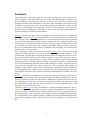
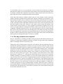
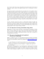
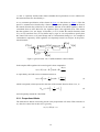
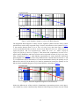
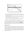
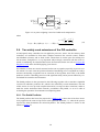
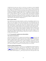
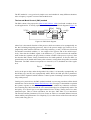
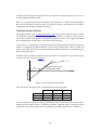
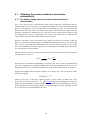
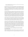
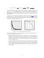
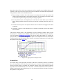
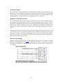
3.1.1. Model based process description
In the great majority of process loops, applying a step to the control variable causes the controlled variable to reach a steady state and does not provoke an instantaneous variation of it.
This means that the process model seen by the regulator can be described by an asymptotically stable, strictly proper transfer function. In a few loops, a control step causes the controlled variable to asymptotically assume a ramp-like behaviour: this case is commonly referred to as ‘runaway’, ‘integrating’ or ‘non self-regulating’ processes and can be described
by models with a pole at the origin of the s-plane. These facts are in good accordance with
experience, since any practitioner would classify the step responses he may encounter more
or less as depicted in Figure 15. Other cases (e.g. an oscillatory response with significant delay) may exist, but they are unlikely to appear in practice. For simplicity, in this section we
do not consider noise and disturbances unless explicitly stated.
Figure 15: classification of step responses.
First-order models
Overdamped responses can be well represented with a first order model plus delay (or ‘dead
time’, leading to the acronym FOPDT), i.e. with a transfer function in the form
e − sL
M (s) = µ
1 + sT
(15)
Many methods exist for identifying such models; an extensive review can be found in chapter 2 of (Åström and Hägglund, 1995). Here we present one of the most widely used, namely
the method of areas. Given the step response record ys(t), one must first compute the gain µ
by dividing the response total swing by the input step amplitude As and the unit step response yus(t) as ys(t)/As. Then, denoting by tend the final experiment time, i.e. assuming that
from tend on yus(t)=µ, it is necessary to compute in sequence the three quantities
A0 =
t end
t0
A0
∫ (µ − y us (t ))dt, t 0 = , A1 = ∫ y us (t )dt
µ
0
32
0