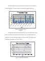
1
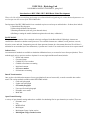
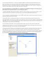
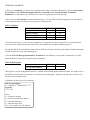
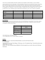
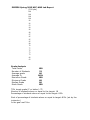
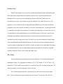
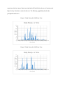
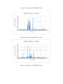
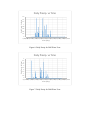
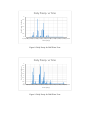
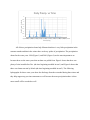
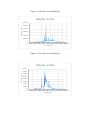
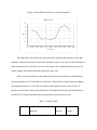
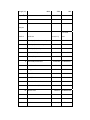
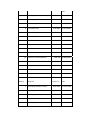
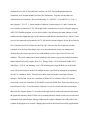
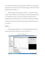
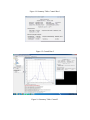
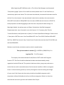
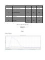
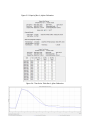
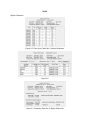
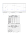
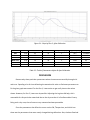
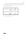
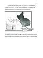
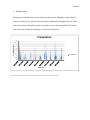
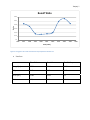
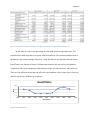
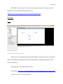
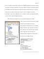
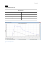
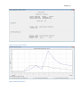
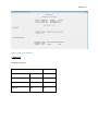
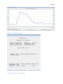
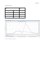
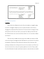
Spring 2015 EGR 356 HEC HMS Lab EGR 356 HEC HMS lab: This lab is on using a hydrologic model to design a system and predict flows. The model is currently used by US army corps of engineers. This assignment addresses the following CE program outcome(s) and performance indicator(s): An ability to identify, formulate, and solve engineering problems (ABET e.) Comments: This was a great lab, and lab reports improved. Suggestions from 2013-2014: Always search for better study site Actions taken: It turned out to be a great site this year. We approached with a different perspective of analyzing the semi-arid are characteristics. It was woven into the class/lab very well. Suggestions from 2014-2015: Always search for better study site where we can go visit. The current site has two water pipes coming in and was shut down after 9/11. HEC-HMS shuts down or erases data when the students try to save the project or run the project. EGR 356L - Hydrology Lab CALIFORNIA BAPTIST UNIVERSITY, spring 2015 Introduction to HEC-HMS: HEC-HMS Basin Model Development This week’s lab will focus on defining and setting up our Basin Model and gathering the various data and parameters we need to input into this section of the HEC-HMS model. Development of the HEC-HMS model for as watershed requires several steps as outlined above. In short, these include: 1) Basin Model Development 2) Meteorological Model Development 3) Running simulations (with our given data and values) 4) Refining or tuning the model simulations against observed data (‘calibration’) BASIN MODEL The physical representation of the watershed or basin is configured in the Basin Model. Hydrologic elements are connected in a network to simulate runoff processes. The available elements are: subbasin, reach, junction, reservoir, diversion, source and sink. Computation proceeds from upstream elements in a downstream direction. We will have 2 subbasins in our watershed (as in our delineation), 1 junction and 1 reach. You can also add a reservoir to capture runoff. Subbasin Loss: As assortment of methods are available to simulation infiltration losses (to account for losses from precipitation). These methods apply only to pervious surfaces. Options for event (single rainfall-runoff storm) include: o Deficit and constant o Green and Ampt o Gridded SCS curve number o Gridded soil moisture accounting o Initial and constant o SCS curve number o Soil moisture accounting Runoff Transformation: Once we have decided on the amount of excess precipitation (from our loss model), we need to turn this into surface runoff. The various methods available within HEC-HMS include: o Clark unit hydrograph o Synder unit hydrograph o SCS unit hydrograph o User-specified unit hydrograph o Kinematic wave model o ModClark Open Channel Routing: A variety of open channel routing methods are available for simulating flow in open channels (or reaches). Thses are: o Kinematic wave o Lag o Modified Puls o Muskingum o Muskingum-Cunge 8 point section o Muskingum-Cunge standard section For each of the procedures above, we will use the designated methods for defining the physical characteristics of our basin. We will need to use our previous and future labs to define the parameters or values that go into each of theses methods that we will use. Your lab this week consists of determining setting up your model “structure”. The goal is to finalize your Basin Model within the HEC-HMS system before spring break. You can download and view the HEC-HMS User’s Manual from our Blackboard to help you with setting up your Basin Model. Do NOT print the manual- it is an extremely large file!!!!! 1) Open the HEC-HMS model system on computer. Under File- open New Project. Give your project a name (i.e. Devil Canyon). Decide where you want to save your model setup. Be sure to select ENGLISH customary units. 2) Go to Components – Basin Model Manager – create a “NEW” model- under your Devil Canyon Project. You can give your basin a name here also (Devil Canyon). 3) Now double click on your Basin Model Folder to see the Devil Canyon Basin Model. Double click on the Devil Canyon Basin Model. This should open a gridded screen (working area) with various tools to design your watershed in the HEC-HMS system. You will need to bring each of the various components into the main screen for your model. Move the cursor (mouse) over the various icons in the display. 4) You will need two sub-basins, as well as a junction and one reach to setup your entire system. Left click on the component you need, then move your cursor to the grid and left click again to place it on the grid. Select create to insert the component on the grid. You can also name each of the components. 5) You will also need to connect each of the subbasins to a junction, junction to a reach and reaches in some order to the outlet. Make sure you have the arrow cursor before proceeding. Connections are then made by left clicking on the component and designation where you want the downstream connection – then right click on the downstream component to connect. Proceed till all the components are connected. There may be several ways to set up the watershed structure, but you should have a model schematic somewhat similar to the figure below. SUBBASIN PARAMETER: 6) Now for each subbasin, you need to select methods for Loss Rate, Transform and Baseflow. Select the SCS method for Loss Rate, the SCS Unit Hydrograph method for Transform and the Constant Monthly for Baseflow Estimation. For each subbasin, you will also need to enter the appropriate area of the drainage. 7) We will use the SCS method to simulate infiltration losses. You will need to define the parameters in each subbasin. These parameters will come mostly from your previous and future labs. SCS Loss Method Parameters Subbasin 1 Area (sq. miles) Initial Loss (inches) 0.5 SCS Curve # (dimentionless) % Impervious ** 1 Subbasin 2 0.5 1 ** For our impervious %, we start with an assumption of 1% impervious for any developed area or exposed bedrocks. You will need to estimate the amount of this area in your subbasin later during the calibration process. To enter the data for the Loss Method- double click on SCS Curve Number link under each subbasin. Initial Abstractions, CN and % impervious entry areas should pop up. 8) For the SCS Unit Hydrograph method for Transform in each subbasin, you will need to calculate the Lag Time parameter basin on our previous length and slope estimations. SCS Unit Hydrograph Parameters SCS Lag Time (Minutes) Subbasin 1 Subbasin 2 This lag time is used as an adjustment factor for a synthetic SCS unit hydrograph within HEC-HMS. The depth of excess precipitation (runoff) will be converted to cfs based on this unit hydrograph – adjusted for the lag time of our basin. We will go over this method in class. Calculations for the various SCS parameters: Time of concentration Tc = 0.00526 L0.8(1000/CN-9)0.7 S-0.5 Lag Time: Tl=Tc/1.67 Where: Tl = Lag time in minutes Tc=time of concentration in minutes L= watershed length in ft S = watershed slope (ft/ft) CN = Curve number for each subbasin 9) We will use Constant monthly for baseflow estimation in each subbasin. For this method, we need to estimate a consistent baseflow value for each month we will run simulations. From the flow records for Devil Canyon, select the low flow values in between precipitation events to estimate a base flow volume for the months of November, December, January, February, March, and April (we will only analyze storms during the rainy season). Since the baseflow at the gage is an aggregate of two subbasins, you will need to estimate a reasonable value for each subbasin. One way to do this would be based on area contribution (take the total baseflow and multiply bye the % area of total for each subbasin). Parameters November December January February March April Total Baseflow Value (cfs) Subbasin 1 Baseflow (cfs) Subbasin 2 Baseflow (cfs) Reach/Routing: 10) For the reaches connection the junction to the outlet, select the Muskingum-Cunge Method. We will make estimates of these channel physics to put into the model and then adjust (if needed) when we calibrate our model to some flow events that have occurred in the canyon. Parameters Shape Length (ft) Energy Slope (ft/ft) * Bottom Width (ft) ** Side Slope (ft/ft) ** Manning's n ** Reach1 PRISM *Use channel slope as a first approximation **Use an approximate value – this may change as we progress. PART 2: After all the values are entered into the Basin Models, we need to add Time-Series data. To do this, go to: Components Time Series Data Manager Data type, select “Precipitation Gages” from the drop down menu Newname it (i.e. DC). Double click on the left hand-side paneldouble click on the gage that you created. And enter the following information: Select the following data table: Under the Time Window Tab: The start date should be 01Oct1997 End Date should be 30Sep2006 Start and End Time is 00:00 Under the “Table” tab, copy and paste all your precipitation data from Lab 1. Create another Time-Series data for discharge: Components Time Series Data Manager for Data Type, select “Discharge gages” from the drop down menu New name it (i.e. DC) Follow the same steps for Discharge data. Basin Model Correction/addition Basin Model Reach -1 Use Manning n: 0.05; Bottom Width of 20ft and side slope of 0.01 Basin model Devil Canyon East Fork select “Options” tab under observed flow, select the flow from DC. Basin model Devil Canyon West Fork select “Options” tab under observed flow, select the flow from DC. Basin model Devil Canyon Junction select “Options” tab under observed flow, select the flow from DC. Basin model Devil Canyon Rea ch-1 select “Options” tab under observed flow, select the flow from DC. **If you have an “Outlet” do the same for the “Outlet”, if you do not have an “Outlet”, you are done. PART 3: Creating Meteorologic Models Go to Components Select “Meteorologic Model Manager” New name it. Double click on the Meteorologic Models on left-hand side panel and click on the component you just created (and named) and enter the following (shown below): Under “Basin” tab Lastly on Option’s tab, input “No” for both Part 4: Control Specifications Manager Go to “Components” and select “Control Specifications Manager” Click “New” and create Control 1 with following storm event Go to “Components” and select “Control Specifications Manager” Click “New” and create Control 2 with following storm event Part 5: Running the HEC-HMS Model Once all your data and storm dates are entered into the model, you are ready to run simulations to get your baseline runs and calibrate your model. Select “Compute” Select “Create a Simulation Run” Name this Run 1 Click “Next” Highlight your basin model (e.g. “Devil Canyon”) and click “Next” Highlight your Met data (e.g. Met 1) and click “Next” Highlight your Control 1 and click “Finish” Select “Compute” Select “Create a Simulation Run” Name this Run 2 Click “Next” Highlight your basin model (e.g. “Devil Canyon”) and click “Next” Highlight your Met data (e.g. Met 1) and click “Next” Highlight your Control 2 and click “Finish” Select “Compute” Select “Select Run” select the run you like to compute. Click on icon to run. The model should now run. If you see warnings-the model ran OK. The warnings are typically associated with the time of concentration or lag time (if our computed time of concentration (Tc) is less than our model time interval or the initial abstractions are unrealistic). If you see errors the model did NOT run and you need to troubleshoot why your model is not running. Check all your start and stop times, and your data entry. Part 6: Viewing Results To view your results, RIGHT click on the OUTLECT JUCTION and go to VIEW RESULTS graph or Summary or Time-series Table. You should see the model simulations for this outlet and the observed flow for comparison to your simulation result graph. Make sure you understand which is the outlet flow. This is the flow that needs to match the “observed” streamflow. Be sure to save your TIME-SERIES for all initial “baseline” runs and final “calibration” runs for each storm. Also be sure to SCREEN CAPTURE THE BASELINE SIMULATIONS you have run before you start your calibrations. Now you can view your results against the observed flow and re-run the model as needed, varying parameter to try and match the observed flow (CALIBRATE YOUR MODEL!) Part 7: Calibrations Boundaries or constraints for parameter values are a “realistic” range of possible parameter values that are determined by the user. Boundaries are set to insure that unreasonable parameter values are not used when searching for “best” values. The HEC-HMS model documentation has a table with realistic values for parameters (HEC HMS User’s Manual, page 133). The optimization procedure is an iterative process. A set of parameters is selected by the user, the model is run, a hydrograph is produced, and the resulting simulation is compared to the observed time series. The process is repeated until an acceptable fit is obtained (correct volume, timing, shape, etc). We have several parameters we can adjust to correct for errors in our simulations. The ones we will primarily focus our calibration on include: Loss Function Parameters: SCS Curve Number % Impervious Initial Loss or Abstraction Constraints 40-100 0-100% 0-20 inches Runoff Transformation Parameters (timing): SCS Lag Time 0-30000 minutes Routing Parameters (Reach 1): Energy Slope Bottom Width Side Slope Manning’s n 0.01-1(?) 0-50 feet 0.01-10 0-1.0 During your calibrations – You should try to capture both the VOLUME of the runoff and the TIMING (or peak) of the runoff (and the shape of the hydrograph). For volume – The SUMMARY RESULTS table shows the observed runoff (inches) and the simulated runoff (inches) – you should try to match these two values as close as possible to get the total storm runoff to be as accurate as possible (< 0.2 inches between these two values preferred, however if you cannot get this close reason what might be the issue, for example, watershed is too small, storm durations are too long to calibrate too, time intervals are large and etc,.). For Timing – The GRAPH of observed vs. simulated will show how well your simulations match the peak flow (your peak should be at the same time period as the observed peak). The parameters that we will change to try and match these two variables are CN, %Impervious and Initial Loss. You can also try changing other parameters, but other parameters are less ‘sensitive (don’t affect the models simulations as strongly)’. You may need different parameters values for each of the storms. BE SURE you keep your parameter values reasonable. Record all final parameter values and save all initial and final simulation data (graphs and tables) to turn in for your final report (FOR ALL STORMS). HEC HMS – Devil Canyon Lab Report Due April 19th, 2011 (Email the lab write-up to [email protected]) ( /100 points) Introduction (10pts) Talk about what hydrologic models do and what model you are using (HEC HMS). Talk about why it is important Study Site (20 pts) Describe your watershed (more details are found on my paper) o Location (state, county…) o Area (in sq mi. is okay) o Weather pattern / discharge pattern Include your precipitation graph from lab 1 Include your hydrograph from lab 1 label the axis, number the figures and explain o Land Use Include your land use classification (lab 2) briefly summarize your table, top two on the list, in your writing Methods (20pts) Include HEC HMS download site Briefly describe the model (consists of basin model, time series model, meteorological model, control specification and run manager) List your inputs (precipitation, observed discharge, and parameters) o Include where and how you obtained the data: USGS.gov (discharge) and San Bernardino Flood Control District (precipitation), and NOAA (land use). How did you obtain CN, Length of watershed, slope, and etc. Results (20 pts) Screen captures of your results (before and after the calibration) Summary Tables of your results (before and after the calibration) Table of parameters (before and after the calibration) Discussion (20 pts) Reason about your parameters: Are your parameters physically reasonable for your watershed? Explain why. Conclusion (10 pts) Is your model accurate and/or precise? What would you improve next time? EGR356 Spring 2015 HEC-HMS Lab Report (100 pts) 100 100 100 100 98 96 93 90 89 88 87 85 85 85 80 78 77 75 73 72 68 62 Grade Analysis Total Points Number of Students Average grade Average % Maximum Grade Minimum Grade Median Grade Mode Grade 100 22 86 86% 100 68 86 100 75% target grade (C or better): 75 Number of students above or equal to the target: 18 Percentage of students above or equal to the target: 82% Goal of percentage of students above or equal to target: 80% (set by the instructor) Is the goal met? Yes. HEC HMS- Devil’s Canyon Lab report Prepared for: Dr. Helen Jung By: Michael Callahan Gordon and Jill Bourns College of Engineering Civil Engineering Department California Baptist University Due 4/22/15 Introduction This lab was meant to be an exercise in creating a hydrological model using the program HEC HMS. The watershed that was modelled was the Devil’s Canyon Watershed in San Bernardino. This exercise was done utilizing the program called HEC HMS which was developed by the Army Corp of Engineers and is available for free online for all to use. This program is a very versatile tool for creating hydrological models for a wide range of different geographic areas, such as urban watersheds, river basins, and flood plains. A hydrological model is a simplified, conceptual representation of a section of the hydrologic cycle and in this case we are modelling the runoff and infiltration of several different times of the water year in an area. Hydrological modelling is important because it is used to help us predict the behavior of a watershed especially during storm events. This allows us to use the information to help mitigate risk by modelling potential flooding and behavior of water that could cause damage in the area. A good example of mitigating risk would be if a bridge was built over the main path of discharge in a watershed, then we can use a hydrological model to help predict the volume of water that would be needed to be able to travel under the bridge safely. Site Study The watershed that was modeled in this lab was the Devil’s Canyon Watershed in San Bernardino County, CA, geographical coordinates of 34°11’52” North, 117°19’54” West. The watershed is 5.5 mi^2 and is separated into a west and east fork. The west fork consisting of 51% of the area and the east fork consisting of 49% of the area. The weather patterns in this area show that most of rain occurs in the winter months (Nov.- Mar.) and that the average rainfall in the area is about 27 in per year. This area also experiences the hot, intense Santa Ana winds in the fall which dries the area of moisture and helps fuel any fires that are started in the area. The following graphs help describe the precipitation in the area. Figure 1: Daily Precip for 1998 Water Year Daily Precip. vs Time 4.5 4 Pre (in/day) 3.5 3 2.5 2 1.5 1 0.5 0 8/8/1997 9/27/1997 11/16/1997 1/5/1998 2/24/1998 4/15/1998 6/4/1998 7/24/1998 9/12/1998 11/1/1998 Times (Days) Figure 2: Daily Precip for 1999 Water Year Daily Precip. vs Time 1.6 Daily Precip. (in/day) 1.4 1.2 1 0.8 0.6 0.4 0.2 0 9/12/1998 11/1/1998 12/21/1998 2/9/1999 3/31/1999 5/20/1999 7/9/1999 8/28/1999 10/17/1999 12/6/1999 Times (Days) Figure 3: Daily Precip for 2000 Water Year Daily Precip. vs Time Daily Precip. (in/day) 2.5 2 1.5 1 0.5 0 8/28/1999 10/17/1999 12/6/1999 1/25/2000 3/15/2000 5/4/2000 6/23/2000 8/12/2000 10/1/2000 11/20/2000 Times (Days) Figure 4: Daily Precip for 2001 Water Year Daily Precip. vs Time 4 Daily Precip. (in/day) 3.5 3 2.5 2 1.5 1 0.5 0 8/12/2000 10/1/2000 11/20/2000 1/9/2001 2/28/2001 4/19/2001 6/8/2001 7/28/2001 9/16/2001 11/5/2001 Times (Days) Figure 5: Daily Precip for 2002 Water Year Daily Precip. vs Time 1.6 Daily Precip. (in/day) 1.4 1.2 1 0.8 0.6 0.4 0.2 0 7/28/2001 9/16/2001 11/5/2001 12/25/2001 2/13/2002 4/4/2002 5/24/2002 7/13/2002 9/1/2002 10/21/2002 Times (Days) Figure 6: Daily Precip for 2003 Water Year Daily Precip. (in/day) Daily Precip. vs Time 5 4.5 4 3.5 3 2.5 2 1.5 1 0.5 0 9/1/2002 10/21/2002 12/10/2002 1/29/2003 3/20/2003 5/9/2003 6/28/2003 8/17/2003 10/6/2003 11/25/2003 Times (Days) Figure 7: Daily Precip for 2004 Water Year Daily Precip. vs Time Daily Precip. (in/day) 3 2.5 2 1.5 1 0.5 0 8/17/2003 10/6/2003 11/25/2003 1/14/2004 3/4/2004 4/23/2004 6/12/2004 8/1/2004 9/20/2004 11/9/2004 Times (Days) Figure 8: Daily Precip for 2005 Water Year Daily Precip. (in/day) Daily Precip. vs Time 5 4.5 4 3.5 3 2.5 2 1.5 1 0.5 0 8/1/2004 9/20/2004 11/9/2004 12/29/2004 2/17/2005 4/8/2005 5/28/2005 7/17/2005 9/5/2005 10/25/2005 Times (Days) Figure 9: Daily Precip for 2006 Water Year Daily Precip. vs Time 4 Daily Precip. (in/day) 3.5 3 2.5 2 1.5 1 0.5 0 9/5/2005 10/25/2005 12/14/2005 2/2/2006 3/24/2006 5/13/2006 7/2/2006 8/21/2006 10/10/2006 11/29/2006 Times (Days) All of these precipitation charts help illiterate that there is very little precipitation in the summer months and that in the winter there are heavy spikes of precipitation. The precipitation charts for the water years 1998 (Figure 1) and 2001 (Figure 4) are the most important to us because these are the water years that our data was pulled from. Figure1 shows that there was plenty of rain in and before Dec. (the time beginning modeled in run 1) and Figure 4 shows that there was almost not rain by March (the time beginning modeled in run 2). The following hydrographs for those water years show the discharge from the watershed during those times and they help support my previous statements as well because the more precipitation there is then more runoff will be recorded as well. Figure 10: 1998 Water Year Hydrograph Daily Dis. vs Time 12000000 Daily Dis (cfd) 10000000 8000000 6000000 4000000 2000000 0 8/8/1997 9/27/1997 11/16/1997 1/5/1998 2/24/1998 4/15/1998 6/4/1998 7/24/1998 9/12/1998 11/1/1998 Times (Days) Figure 11: 2001 Water Year Hydrograph Daily Dis. vs Time 1600000 Daily Dis. (cfd) 1400000 1200000 1000000 800000 600000 400000 200000 0 8/12/2000 10/1/2000 11/20/2000 1/9/2001 2/28/2001 4/19/2001 6/8/2001 7/28/2001 9/16/2001 11/5/2001 Times (Days) Figure 12: Runoff Ratio for Devil’s Canyon Watershed RR vs Year 0.6 0.5 RR 0.4 0.3 0.2 0.1 0 1997 1998 1999 2000 2001 2002 2003 2004 2005 2006 2007 Time (years) This chart shows the runoff ratio in the area and it illustrates that amount of water that infiltrates compared to how much water runs off in those years. As we can see, the runoff ratio is relatively high for the 1998 water year so we can expect a lower initial abstraction and we can expect a higher initial abstraction than in the 2001 water year. This is a semi-arid climate so the majority of the plant life consists of scrub and shrub which encompasses 62% of the land use in this area. Some mixed evergreen forest is at higher elevations and consists of 31% of the area. Both of these land uses have relatively low Cn numbers because they do not prevent infiltration. The table below descripts all of the land uses for the Devil’s Canyon Watershed and also shows how much area each covers. Table 1: Land Use table Gate to West Fork East Fork Junction length (m) 4860 slope (%) 2760 800 16.46090535 10.86956522 12.5 Devil Canyon % of Total Code # Land Use Area (m^2) 3 Developed, Medium intensity Area 6126.31 0.043006937 4 Developed, Low intensity 130516.48 0.916230812 5 Developed, Open Space 148547.77 1.042811175 6 Cultivated Crops 8710.36 0.061147069 7 Pasture/Hay 1483.28 0.010412684 156162.89 1.096269617 9 Deciduous Forest 17791.89 0.124899766 10 Evergreen Forest 4327085.4 30.37630933 11 Mixed Forest 791680.59 5.557628813 12 Scrub/Shrub 8790593.12 61.71030871 13 Palustrine Forested Wetland 2732.8 0.019184363 14 Palustrine Scrub/Shrub Wetland 741.85 0.005207816 12616.12 0.088565658 8 Grassland/Herbaceous 20 Barren Land West Fork Code # Land Use Area (m^2) % of Total Area 3 Developed, Medium intensity 3124.4181 0.021933538 4 Developed, Low intensity 66563.4048 0.467277714 5 Developed, Open Space 75759.3627 0.531833699 4442.2836 0.031185005 756.4728 0.005310469 79643.0739 0.559097505 9 Deciduous Forest 9073.8639 0.063698881 10 Evergreen Forest 2206813.554 15.49191776 11 Mixed Forest 403757.1009 2.834390695 12 Scrub/Shrub 4483202.491 31.47225744 13 Palustrine Forested Wetland 1393.728 0.009784025 14 Palustrine Scrub/Shrub Wetland 378.3435 0.002655986 6434.2212 0.045168485 6 Cultivated Crops 7 Pasture/Hay 8 Grassland/Herbaceous 20 Barren Land East Fork % of Total Code # Land Use 3 Developed, Medium intensity Area (m^2) Area 3001.8919 0.021073399 4 Developed, Low intensity 63953.0752 0.448953098 5 Developed, Open Space 72788.4073 0.510977476 4268.0764 0.029962064 726.8072 0.005102215 6 Cultivated Crops 7 Pasture/Hay 8 Grassland/Herbaceous 76519.8161 0.537172112 9 Deciduous Forest 8718.0261 0.061200885 10 Evergreen Forest 2120271.846 14.88439157 11 Mixed Forest 387923.4891 2.723238118 12 Scrub/Shrub 4307390.629 30.23805127 13 Palustrine Forested Wetland 1339.072 0.009400338 14 Palustrine Scrub/Shrub Wetland 363.5065 0.00255183 6181.8988 0.043397172 20 Barren Land Methods Procedure listed in the lab: 1.) Basin Model Development 2.) Meteorological Model Development 3.) Running Simulations 4.) Calibration The model program used in this lab was HEC HMS which can be downloaded for free at: http://www.hec.usace.army.mil/software/hec-hms/downloads.aspx. In this program we create a physical representation of the watershed, which is called a basin model, using different elements like subbasins and reaches. These elements are connected in a network to simulate runoff processes. The Devil’s Canyon watershed included 2 subbasins, 1 junction and 1 reach. The model also consists of a time series model, meteorological model, control specifications, and run manager. Next the parameters and methods to be used needed to be input into the model. The model used U.S customary units throughout and the SCS curve number method was selected for both the subbasin loss and runoff transformation in our model while the Muskingum-Cunge standard section was used for our open channel routing. Each subbasin then needed to be configured to use the SCS method for Loss Rate, the SCS Unit Hydrograph method for Transform, and Constant Monthly for Base flow Estimation. Lag time was needed to be calculated for the Transform. This was done using Tc= .00526*L^.8 *((1000/Cn-9)^.7)*S^-.5 then Lagtime = Tc/1.67. L means length of subbasin, S means slope in %, and Cn means the curve number (assumed to be 70). The length of the watershed was found by using the program ARC GIS. With this program we were able to make a line following the main tributary in each subbasin and the length and slope of the subbasin would then be calculated for us. Initial Cn was given by the instructor and assumed to be 70. My initial calculated lagtime for the West fork was 126.44 minutes and 98.93 minutes for the East fork. The base flow for each basin was then estimated to be the lowest discharge value in each month that the model was running and dividing that value by the percent of area each subbasin covers to get a base flow for each subbasin. The reach connection from the junction to the outlet was given the initial parameters: Shape=Prism/Trapezoid, Length=2624.67 ft, Energy Slope=.125 ft/ft, Bottom Width= 20 ft, Side Slope= .01 ft/ft, and Manning´s n 0.3. The Muskingum-Cunge Method was used for the reach. The meteorological model was configured to be a specified hyetograph in precipitation, also in U.S. customary units. Two runs were then created using the control specification manager. The first run was to use a start date of 04Dec1997 to end date 16Dec1997 and the second run was to use a start date of 23Feb2001 to end date 05Mar2001. Each run needs to use a time interval of 1 day. To run the model, either run 1 or run 2 was selected in the run manager then click the compute button. To view the results right clicked on the outlet junction and select the graph and summary tables. If there are no warnings then the initial results were recorded and calibration of the model began. During calibration, the lagtime changed where the peaks of the synthetic hydrograph were located. Changing the baseflow raised and lowered the graph and the Cn and initial abstraction flatten out the graph. The goal of calibration was to get the synthetic hydrograph as close to but still above the real measured hydrograph. Calibration could stop once the total residual was less than .2 in. Data like precipitation, observed discharge, and land use, were pulled from multiple locations to make modeling the area possible. Discharge was found using information form the U.S. Geological Survey website, www.usgs.gov. Precipitation was found from the San Bernardino Water Control District website, www.sbcounty.gov/dpw/floodcontrol/default.asp. The land use was found from the National Oceanic and Atmospheric Administration website, www.noaa.gov. Results The following graphs and tables are a result of changing different parameters in the hydrological model until the total residual was equal to or less than .2 in. Figure 13: Control Run 1 Figure 14: Summary Table: Control Run 1 Figure 15: Control Run 2 Figure 16: Summary Table: Control 2 Figure 17: Calibrated Run 1 Figure 18: Calibrated Run 1 Summary Table: Figure 19: Calibrated Run 2 Figure 20: Summary Table: Calibrated Run 2 Table 2: Table of Parameters: Before and After Before (run 1) Int Abs Cn Imp % Baseflow (cfs) Lagtime (min) Before (run 2) Int Abs Cn Imp % Baseflow (cfs) Lagtime (min) West East Run 1 0.5 0.5 Int Abs 5 5 Cn 1 1 Imp % Baseflow 0.1071 0.1029 (cfs) Lagtime 126.44 98.93 (min) West East Run 2 0.5 0.5 Int Abs 5 5 Cn 1 1 Imp % Baseflow 1.02 0.98 (cfs) Lagtime 126.44 98.93 (min) West East 0.77 15 1 0.77 15 1 0.8 0.6 126.44 98.93 West East 7.2 2 4.15 7.2 2 4.15 3.7 3.7 100 50 Discussion The parameters listed above are supposed to be used to realistically model the behavior of the watershed that was model. The parameters for the first run do seem physically reasonable for Devil’s Canyon other than the Cn is too low. The Cn is 15 when a physically reasonable Cn number should be between 40-100. The lag time however matched the time that was calculated with the information that was given about the watershed like length and slope. The initial abstraction was a little bit higher but so was the base flow in the area then initially calculated. This physically makes sense because the base flow for the area was initially calculated to be very small. The parameters for the run 2 however do not physically make sense. Both the initial abstraction and the base flow are significantly higher. A higher initial abstraction does not make sense in this case because the area has a much higher impervious %. Also a higher initial abstraction rate usually results in a greater lag time but the lag time in run 2 is shorter than run 1. Also the Cn number is incredibly low and during calibration the Cn number seemed to be doing little to nothing to the model if it was anywhere from 75 down to 5. These inaccuracies in the second run are likely due to the little amount of data that was available to calibrate. This run was done during a dry spell so there was almost no rainfall or runoff that could be used in the modeling. Conclusion In this lab we calibrated two different models for the Devil’s Canyon watershed. Run 1 was done using information gather about the watershed in December and the second run was done in late February and early March. Both runs do not make sense physically because of the Cn numbers. To make the calibration more accurate next time I would start with a higher Cn number like 60 and start calibrating around that instead of starting with a low number, I started calibrating with an assumed Cn value of 5. I would also say the model was not very precise because it was only using information from one year for each run and there are a lot of uncertainty in hydrological modeling like inaccuracy of rain measurements or area calculations. The calibrated values of the second model do not physically make sense for the area and this probably do to the low amount of information that was available for the watershed at this time of the year. To make these models more accurate for next time I would chose several winter month from different years with higher precipitation so a comparison can be made from the different data that could be modeled from several years. This could also help make a more an accurate model because multiple similar runs would be done and we would not run into the difficulty of the drier model. Also I would try to find a way to save the HEC HMS files better because a lot of trouble was experienced trying to make sure your data was not lost. CALIFORNIA BAPTIST UNIVERSITY COLLEGE OF ENGINEERING EGR 356: Hydrology Devil’s Canyon Basin Hydrological Model Prepared for: Dr. Jung By: Steven Bell 491338 April 22, 2015 INTRODUCTION For this assignment, HEC HMS was used. The Hydrologic Modeling System (HEC-HMS) is designed to simulate the complete hydrologic processes of dendritic watershed systems. The software includes many traditional hydrologic analysis procedures such as event infiltration, unit hydrographs, and hydrologic routing. For our design, we were able to develop a model to convert rainfall volume into runoff volume. A runoff curve number is a parameter that was used to predict the direct runoff and rainfall excess. Specific values had originally been given to the class in order to start the model; however, we were to calibrate until the total residual was less than 0.2. Below is an image depicting the original constraints. Figure 1.1: Constraints for original lab HEC- HMS is a valiant resource that can provide the following: Precipitation-specification options which can describe an observed (historical) precipitation event, a frequency-based hypothetical precipitation event or an event that represents the upper limit of precipitation possible at a given location; Loss models that can estimate volume of runoff, given the precipitation and properties of the watershed; direct runoff models that can account for an overland flow, storage and energy losses as water runs off a watershed into the stream channels; hydraulic routing models that account for storage and energy flux as water moves through stream channels; models of naturally occurring confluences and bifurcations; Models of water-control measures including diversions and storage facilities. There are countless benefits that HEC-HMS provides to civil engineers that help with everyday living and strive to make an overall better world for everyone to live in. Figure 1.2: HEC-HMS Model for Devil Canyon STUDY SITE Devil Canyon watershed is located in the San Bernardino Mountains, approximately 75 miles east of Lost Angeles. It is a steep sided canyon on the south side of Paivia Peak, in San Bernardino County. The Canyon’s two forks, East and West, are tributary of the Santa Ana River watershed. Devil’s Canyon has two primary tributaries, the West Fork and East Fork. The watershed includes 2 sub-basins, one junction, one outlet and one reach. Majority of drainage occurring throughout the basis is due to the West Fork. East and West Fork of the Canyon contain five primary soil types; however, the West Fork includes three additional types of soil. Clay loam and exposed bedrock are also noted to be found in the West Fork. Figure 1.3: San Bernardino County Figure 1.4: Devil’s Canyon, San Bernardino CA Devil Canyon is a populated area located in San Bernardino County at latitude and longitude (34.198, 117.333) and an elevation of 1,785 feet above sea level. The total area of this watershed of Devil Canyon is 5.2 mi². This area is a mountain area. It rains mostly during the winter. It has a semi-arid climate that receives precipitation below potential evapotranspiration. Devil Canyon has a perennial stream that has continuous flow in parts of its stream bed all year round during years of normal rainfall. Figure 1.5: Topographic Map of Devil’s Canyon The southern California region has a semi-arid climate, with rainfall averaging from 368 mm/yr. in downtown Los Angeles to 990 mm/yr. in the surrounding mountains. Precipitation rarely occurs, however when it does so, it occurs from November to March. It has a semi-arid climate that receives precipitation below potential evapotranspiration, but not extremely. Devil Canyon has a perennial stream that has continuous flow in parts of its stream bed all year round during years of normal rainfall. The following graph represents the precipitation obtained from San Bernardino Flood Control district. The graph shows the precipitation throughout eight years. gr Precipitation Pre Figure 1.6: Precipitation Graph from Lab 1 The figure below describes the Watershed Runoff ratio from 1998 to 2006. Factors that can contribute to the runoff ratio are duration of storm, topography (slope) and evaporation. The Year containing the highest runoff ratio is 2005. This is due to more precipitation and wildfires, such as the “Old Fire.” off Ratio W er e R Figure 1.7: Watershed Runoff Ratio METHODS Materials/Equipment 1. ARC GIS, used to obtain original data 2. HEC-HMS HEC-HMS was downloaded from the following: http://www.hec.usace.army.mil/software/hec-hms/download.html The following description gives brief information on each symbol that is used to represent individual hydrologic element. Figure 1.8: Sample tools within HEC-HMS Procedure Our basin model was set up by gathering the various data and parameters needed to run it. There were several steps required in this procedure: 1) 2) 3) 4) Basin Model Development Meteorological Model Development Simulations Refining and Calibration of model simulations Basin Model Development The discharge was obtained from http://waterdata.usgs.gov/ca/nwic. The precipitation was obtained from San Bernardino Flood Control District http://www.co.sanbernardino.ca.us/dpw/floodcontrol/water_resources.asp; and the Land use from NOAA. Basin Method: the physical representation of the watershed or basin is configured in the Basin model. Hydrologic elements are connected in a network to simulate runoff processes. In the subbasin loss the SCS curve number option was chosen. In the Runoff Transformation, the SCS unit hydrograph option was chosen. In the Open Channel Routing, the Muskingum-Cunge standard section option was chosen. When calculating, first the time of concentration and lag time was to be calculated, then the curve number. The curve number was calculated from CN=1000/(10+S) as 66 and then was calibrated according to the graphs in order to find the best fit. Figure 1.9 The calculated values that were originally solved for are shown below and were used when initially setting up HEC-HMS for use. CN 79 75 75 85 69 80 60 61 61 67 67 66 85 x 0.38499 6.432749 1.973684 0.579922 0.134503 5.302144 1.169591 16.58772 13.31774 19.06823 0.195906 0.064327 0.82846 66.03996 CN (I)= CN (III)= 42.63303599 81.7007535 ΣCN (II)= 66 Figure 1.10: Calculated values for CNI, CNII, & CNIII Length of the water running through the basin was found using the ARC GIS. The “elevation” layer was chosen as the top layer. Click on Start from the gage to the top. Follow the lowest points on west fork. The elevation map (DEM) was taken from www.seamless.usgs.gov. Slope was found by using the ARC GIS. The “elevation” layer was chosen as the top layer. Click on info icon. Click on a contour line near the gage and another at the highest point. Slope of the watershed= [(Elevation high- Elevation low)/ Watershed Length] Watershed Length (m) Slope West East Devil Canyon West Fork East Fork Length (ft) Length (ft) 6126.7 6126.7 3939 20100.72 12923.23 0.130576 0.130576 0.101549 Figure 2.0: Depiction of Length & Slope of Watershed When beginning HEC-HMS data series, a Time Series Data Manager must be opened. “Precipitation gauges” option is first used from the drop down menu. To use Data Source, a manual entry option was chosen. The units were then selected; Incremental inches were used for this lab. For a time interval, 1 day was selected. Under the time window, time was started at 01Oct1997 and ended on 30Sept2006. Start time was at 00:00 and end time was at 00:00. For both precipitation and discharge gauges, data from lab 1 was placed in table settings. For Metrologic Models, the settings were as follows; Precipitation: Specified Hyetograph Evapotranspiration: none, Snowmelt: none, Unit System: U.S. Customary, Bain Tab: Yes *include Sub-basins, and Options tab: no (both). For Control Specification Manager: Create control 1. Description: 1997 Dec storm. Start Date 04Dec1997. Start Time: 00:00. End Date 16Dec1997. End Time: 00:00.Time Interval: 1day. Create Control 2 and do the same but date 23 Feb 2001 and end date 05Mat2001. Below are some further calculations used to solve for needed values. Time of concentration in minutes (Tc) = 0.00526L0.8 (1000/CN-9)0.7 S-0.5 Lag time (T1) = Tc /1.67List inputs The majority of the watershed was Scrub/Shrub at 28.5% while and Evergreen forest at 27%. The Class Scrub-Shrub Wetland includes areas dominated by woody vegetation less than 20 feet tall. The species include true shrubs, young trees, and trees or shrubs that are small or stunted because of environmental conditions. While an evergreen forest is a forest consisting entirely or mainly of evergreen trees that retain green foliage all year round. Such forests rein the tropics primarily as broadleaf evergreens, and in temperate and boreal latitudes primarily as coniferous evergreens. Below is a chart that describes the land cover type that was located in Devil Canyon. Land Cover Type 3 4 4 6 7 8 9 10 11 12 13 14 20 Description Developed Medium Intensity Developed low intensity Developed low intensity Cultivated Corps Pasture/Hay Grassland/Herbaceous Deciduous Forest Evergreen Forest Mixed Forest Scrub/Shrub Palustrine Forested Wetland Palustrine Scrub/Shrub Wetland Barren Land total= Area (m^2) 5 88 27 7 2 68 20 279 224 292 3 1 10 1026 Table 2.1: Land Cover Type Chart RESULTS RUN 1 Before Calibration area 0.00 0.09 0.03 0.01 0.00 0.07 0.02 0.27 0.22 0.28 0.00 0.00 0.01 1 % area 0.49 8.58 2.63 0.68 0.19 6.63 1.95 27.19 21.83 28.46 0.29 0.10 0.97 100 Figure 2.2: Graph of Run 1, before Calibration Figure 2.4: Time Series Table Run 1, After Calibration RUN 2 Before Calibration Figure 2.5: Time Series Table Run 2, Before Calibration Figure 2.6 Figure 2.7: Summary Table Run 2, Before Calibration Figure 2.8: Graph of Run 2, Before Calibration After Calibration Figure 2.9: Time Series Table Run 2, After Calibration Figure 2.10: Summary Table Run 2, After Calibration Figure 3.1: Graph of Run 2, After Calibration East West East run 1 West run 1 East run 2 West run 2 Area 2.97 2.53 2.97 2.53 2.97 2.53 Initial Abstraction 0.5 0.5 10 10 10 10 Curve Number 79 79 40 40 95 95 Impervious (%) 1 1 3 3 4.5 4.5 Lag time (min) 42.2 52.12 850 1450 1300 1300 Table 3.2: Table of Parameters before & after Calibration DISCUSSION Reasons why these particular parameters where chosen were essentially through trial and error. Spending a lot of time calibrating the watershed in order to find exact parameters to fit the given graph was wasted. For the Run 1, it was easier to get really close to the values shown. However, for Run 2, it was near impossible. Adjusting the Lag time did help; this is reasonable for this particular watershed due to the dry area that is in San Bernardino County. Being such a dry area, the soil was not very saturated and was permeable. Since the parameters that affect the curve are the CN, %Impervious, and Initial Loss those are the parameters that were mostly changed during calibration. Also, the base flow had Base Flow 1.129998 0.962591 0.5 0.5 3.5 3.5 to be adjusted so that the two graphs would be closer to each other. CONCLUSION In conclusion, the model that was created was both accurate and precise. For this design, I was able to develop a model to convert rainfall volume into runoff volume. Specific values had originally been given to the class in order to start the model. After competing calibration, I was able to get a total residual value less than 0.2. Overall, I had fun once I was able to start calibrating; but the set up phase, excel portion, etc. all took up so much effort and time. I was originally confused with the set up but after dealing with it for an extended amount of time, I was able to understand the overall concept of HEC-HMS. If I had to choose something to improve on next time, it would be my efforts to understand the program from the beginning. I would definitely invest more time and effort into grasping the overall concept. Through this assignment, I learned a lot about hydraulic modeling and look forward to using HEC-HMS in the future. REFERENCES Jung, Helen Y., Terri S. Hogue, Laura K. Rademacher, and Tom Meixner. "Impact of Wildfire on Source Water Contributions in Devil Creek, CA: Evidence from End-member Mixing Analysis." Diss. University of California Los Angeles, 2008. Abstract. "HEC-HMS." Hydrologic Engineering Center Home Page. Web. 18 Apr. 2014. <http://www.hec.usace.army.mil/software/hec-hms/>. “HMS.” Hydraulic Modeling System. Web. 21 Apr. 2014. <http://www.hec.usace.army.mil/software/hec-hms/documentation/HECHMS_Technical%20Reference%20Manual_(CPD-74B).pdf>. Hydraulic Analysis and Modeling. Web. 21Apr. 2014. http://www.hazenandsawyer.com/work/services/hydraulic-modeling-and-analysis/. Thaipejr 1 EGR 356 HYDROLOGY HEC HMS Hydrological Model For: Dr. Jung By: Jom Thaipejr 04/20/2015 Thaipejr 2 Abstract: The purpose of this lab is to understand the hydrological cycle’s characteristics of a watershed area. In this lab data is taken from various government agencies including the application used. Introduction: The hydrologic model, a simplified version of nature’s hydrologic cycle in which scientists and engineers can use to observe the effects of rain to a specific area. Although this is a hard task to perform, with the advancement of technology with new tools and equipment, studying these models are now easier. For this specific lab we will simulate a study on Devil’s Canyon located in San Bernardino in California. With this specific area in mind the data with the type of land in that area along with the precipitation in past years will be obtained from various government agencies. These agencies include the San Bernardino Flood Control, National Oceanic and Atmospheric Administration (NOAA), and ArcGIS. The application that will be used to create the hydrologic model is called the Hydraulic Engineering Center – Hydrologic Modeling System (HEC – HMS). Made and used by the U.S. Army Corp of Engineers. Thaipejr 3 Students work king on this lab will use HEC – HM MS to turn raiinfall volume obtained fr from the various agencies into runoff volume. v Theen they will bbe expected to calibrate their model he constraintss set by the professor. p within th Figure 1: Pa arameters and C Constraints durin ng Calibration Study Siite: Thaipejr 4 The T location that t will be used u in this lab will be D Devil Canyoon in San Berrnardino, Californiia (34°12′53″N 117°19′4 43″W). This area is a moountainous reegion withinn the San Bernardin no Mountain ns close to California C Staate Universiity San Bernnardino. West Fork East Fork Junnction Figure 5: Th he location of De evil Canyon in California The regio on use to be open for pub blic access, but b ever sincce the 9/11 iincident the area is now off limit to th he public beecause of its importance as one of thee many sourrces of waterr to this regioon. Thaipejr 5 Figure 6: To opo map of Deviil Canyon As seen above a the area consists of o steep mou untains that ccan reach thee elevation oof 1,785 feett above seaa level. The region is maade up of tw wo forks and a junction w where the twoo forks meett. Its total area a is 5.2 mi m 2 with the West W Fork co overing 51% % of that areaa. The regionn also is madde up of variou us soils that affect a how much m water is absorbed iinto the grouund. Thaipejr 6 Weather Pattern The amount of rain this area receives is based on the seasons. During the summer Devil’s Canyon is relatively dry, but the stream does flow continuously throughout the year. When winter arrives that is when this region is expected to receive the most rainfall. This winter time is between October thru February as seen in the chart below. Precipitation (in.) Precipitation 5 4.5 4 3.5 3 2.5 2 1.5 1 0.5 0 Precipitation Time ( yr) Figure 4: This graph shows the amount of precipitation in the time frame set for this lab. Thaipejr 7 Runoff Ratio 0.6 0.5 Ratio 0.4 0.3 0.2 0.1 0 1996 1997 1998 1999 2000 2001 2002 2003 2004 2005 2006 Time (Years) Figure 5: This graph is the runoff ratio based on the precipitation and flow rate. Land use: West Fork East fork Devil’s Canyon Length [m] 5520 3304 8824 Slope 0.12 0.12 0.12 Area [mi2] 2.805 2.695 5.5 % Area 49% 51% 100 % Thaipejr 8 Figure 4: This is the land use chart and the three last digits at the bottom is the percentage of total land use. In this chart you can see the percentage on what kind of land occupied that area. The model has been broken up into its two parts with West and East. The last three numbers seen at the bottom is the total percentage of land use. Using this data we can determine the runoff ratio. Runoff ratio is the function of water’s different interactions to this area such as precipitation, evaporation, and evapo-transpiration with relation to slope, soil characteristics, and land cover. There are also different factors that can affect this ratio with how often it rains, slope of the area, and how much water infiltrates or evaporates. Runoff Ratio Ratio 0.6 0.4 0.2 0 1996 1997 1998 1999 2000 2001 Time (Years) Figure 5: Runoff Ration Chart 2002 2003 2004 2005 2006 Thaipejr 9 Methodss: Materialss/Equipmentt: 1. ARC GIS is i used to ob btain the dataa that is will be used to w with the hyddrological moodel. Figure 6: Co ompany logo forr ArcGIS 2. HEC HMS S- 3.5 is the application a that t is used tto make the m model. Figure 7: Website to downlload HEC HMS. Thaipejr 10 HEC HMS as seen in figure 5 has been made and provides by the US Army Corps of Engineers. Link to download this application is here. (http://www.hec.usace.army.mil/software/hec-hms/downloads.aspx ) Procedure: Model: Figure 8: The model made inside HEC‐HMS. Basin model is developed using the tools HEC-HMS provided and the data was obtained data from multiple government sites that provides discharge, precipitation, and land use data. Sites are listed below. Discharge: http://waterdata.usgs.gov/ca/nwic Precipitation: http://www.co.san-bernardino.ca.us/dpw/floodcontrol/water_resources.asp Land Use: www.csc.noaa.gov/landcover Thaipejr 11 Time series model is the data thaat is inputted d into HEC H HMS regardiing the preciipitation thatt has taken plaace on each day d for that season. s Thiss leads into thhe meteoroloogical modeel which usess the data from m the junctio on that conneects both fork ks where thee precipitatioon takes placce. To preveent getting unnecessary data d sectionss within the graph, we w will be focusiing on the coontrol specificaations. Lastly y is the run manager m wheere we look aat two runs bbased on twoo controls annd two time windows on n precipitatio on and disch harge. Even E with thiis data the model m is not yet y ready to rrun and prodduce the resuults. Under U each tab for both West and E East fork, it nneeds a little bit m more informat ation than jusst the precipitation p n data. The m model needs curve numbber, length l of waatershed, sloppe, and otheer data. Manyy of these t valuess have been ccalculated inn previous laabs. The T few valuues that werre still needeed to be calculated c foor the SCS pparameters. T The formulaas used u can be seen in Figuure 10 below w. Figure 9: D Data manager in n HEC‐HMS Figure 10: Formula to find lag time an nd concentration n time. Thaipejr 12 Results: Initial Parameters for Run 1 & 2: West & East Fork Initial Abstraction .5 Curve Number 50 Impervious 1.0 Lag Time 51.22 Figure 11: Initial Graph for Run 1 Thaipejr 13 Figure 12: Summary for Initial Run 1 Figure 13: Initial Graph for Run 2 Thaipejr 14 Figure 14: Summary for Initial Run 2 Calibrated: Calibration for Run 1 West East Initial Abstraction 3 1.065 Curve Number 40 40 Impervious 1.5 .9 Lag Time 50 50 Thaipejr 15 Figure 15: Run 1 Graph after Calibration Figure 16: Summary for Run 1 after Calibration Thaipejr 16 Calibrations for Run 2 West East Initial Abstraction 1 1 Curve Number 40 40 Impervious 5 5 Lag Time 50 50 Figure 17: Run 2 Graph after Calibration Thaipejr 17 Figure 18: Summary for Run 2 after Calibration Discussion: The main objective during calibrations is to align the blue and black line as close and possible with keeping the total residual (seen in summary results) less than 0.2. The constraints during calibration are listed below. These values help adjust to correct possible errors in our simulation. Thaipejr 18 Figure 19: C Constrains durin ng calibration Conclusiion: In n this lab after the calibrrations the reesults of the total residuaal were accepptable stayinng less than 0.2. Althoug gh the calibrration processs was mostlly trial and eerror which iis done by g values with hin both the West W and Eaast fork. Thee values that had to be chhanged weree the changing initial parameters succh as the currve number, percent imppervious, andd many otherrs. Both runss after calibration becaame more accurate than initially, i butt there were a few issuess that could hhave been corrrected. The T values th hat are includ ded in this laab from past labs could hhave been doone better. D Due to lack off knowledgee of knowing g that this HE EC-HMS labb relies on past lab data, I felt could have been don ne better. Datta from past labs could have h been innaccurate duee to human eerror while performin ng calculatio ons and researching wheere the sourcce of some nuumbers weree. This does not deter the fact that this lab was su uccessful in producing p daata based on the Devil C Canyon modeel. Even afteer calibration n the data on n the model only o becamee more accurrate than how w it was inittially.