1
MÄLARDALEN HOGSKOLA UNIVERSITY
School of Innovation, Design and Engineering
Thesis work
SIMULATOR ORIENTED CONTROL OF POWER IN
BLUETOOTH WIRELESS SENSOR NETWORKS.
Manuel García Plaza
Francisco Javier Chicharro Martin
2009
1
MÄLARDALEN HOGSKOLA UNIVERSITY
School of Innovation, Design and Engineering
Thesis work
SIMULATOR ORIENTED CONTROL OF POWER IN
BLUETOOTH WIRELES SENSOR NETWORKS.
Students:
MANUEL GARCÍA PLAZA
FRANCISCO JAVIER CHICHARRO MARTIN
Supervisor:
Martin Ekström ( [email protected] )
Mikael Ekström ( [email protected] )
Qualification: .........................................................................................
Dates: .…....................................................................................
2
GENERAL INDEX
GENERAL INDEX ............................................................................................................................. 3
Index of images .................................................................................................................. 8
Index of Tables ................................................................................................................. 11
I. Abstract .......................................................................................................................................... 12
II. Introduction ................................................................................................................................... 13
1. Context ......................................................................................................................... 13
2. Specific objectives of the project.................................................................................. 15
2.1 Objective................................................................................................................. 15
2.2 Specification ........................................................................................................... 15
3. Description of the work ................................................................................................ 17
4. Methodology and plain of work ................................................................................... 18
5.
Structure of the document ........................................................................................ 19
III. BACKGROUND ......................................................................................................................... 20
CHAPTER 1. THEORETICAL CONTEXT ..................................................................................... 20
1.1.
Theory about Wireless Sensor Networks ............................................................... 20
1.1.1. Introduction Wireless Network .......................................................................... 20
1.1.2. Wireless Sensor Network ................................................................................... 23
1.2.
Theory simulation of networks. ............................................................................. 25
1.2.1. Characteristics and simulation models ............................................................... 25
1.2.2. When it is proper to simulate? ............................................................................ 27
1.2.3. Uses of network simulators ................................................................................ 27
1.3.
Existing Simulators ................................................................................................ 28
1.3.1. OMNeT++ .......................................................................................................... 28
1.3.2. Realistic and Large Network Simulator (Real) .................................................. 28
3
1.3.3. Java -Simulator ................................................................................................... 28
1.3.4. Wireless IP Simulator (WIPSIM) ....................................................................... 29
1.3.5. NS2 with the extension of Bluetooth:................................................................. 29
1.3.5.1. Ns2 extension UCBT ................................................................................... 30
1.3.5.2. Ns2 extension BlueHoc ............................................................................... 31
1.3.5.3. Ns2 extension BlueWare ............................................................................. 31
1.4.
Study of the simulator currently used more. NS2 .................................................. 32
1.4.1. Introduction ........................................................................................................ 32
1.4.2. Installation and Problems (*).............................................................................. 32
1.4.2.1. Cygwin ........................................................................................................ 33
1.4.2.2. Virtual Machine ........................................................................................... 35
1.4.2.3. Problems ...................................................................................................... 36
1.4.3. Basic Procedure of Work.................................................................................... 36
1.4.3.1. Post processing ............................................................................................ 37
1.4.3.2. View of results ............................................................................................. 37
1.4.3.3. Source Code TCL Example ......................................................................... 37
1.4.3.4. Out Nam Example ....................................................................................... 38
1.4.3.5. X Graph Example ........................................................................................ 38
1.5.
Study Bluetooth wireless sensor network technology ........................................... 39
1.5.1. Introduction Bluetooth........................................................................................ 39
1.5.3. Basic functioning. ............................................................................................... 40
1.5.4. Architecture of Bluetooth. .................................................................................. 42
1.5.4.1. Specter of frequencies. ................................................................................ 42
1.5.4.2. Outline of multiple access. .......................................................................... 42
1.5.4.3. Communication based on packet transmission............................................ 42
4
1.5.4.4. Physical connections ................................................................................... 44
1.5.4.5. Establishment of the connection .................................................................. 44
1.5.4.6. Administration of the energy ....................................................................... 44
1.5.4.7. Sniff mode ................................................................................................... 45
1.5.4.8. Interconnection of piconets ......................................................................... 47
1.5.5. Standardization of Bluetooth .............................................................................. 47
1.5.6. Version 2.0+EDR ............................................................................................... 48
CHAPTER 2. PROPERTIES OF THE PROGRAM ......................................................................... 49
2.1. The simulator ......................................................................................................... 49
2.2. Structure of files .................................................................................................... 51
2.3. Errors in the simulation ......................................................................................... 52
2.4. Help ....................................................................................................................... 52
2.5. Premises of the simulator ...................................................................................... 53
CHAPTER 3. MAIN FUNCTIONS .................................................................................................. 54
3.1. Help of Simulator Wireless Sensor Network ........................................................ 54
3.2. Help of Nodes ........................................................................................................ 57
3.3. Help of Characteristic ............................................................................................ 59
3.4. Help of Events ....................................................................................................... 61
3.5. Help of Graphic ..................................................................................................... 63
3.5. Help of Table ......................................................................................................... 65
3.6. Help of Characteristic Node .................................................................................. 67
CHAPTER 4. AUXILIARY FUNCTIONS IN DEPTH ................................................................... 69
4.1. Dates ...................................................................................................................... 69
4.2. DrawGraphic ......................................................................................................... 69
4.3. DrawNetwork ........................................................................................................ 71
5
4.4. Routing .................................................................................................................. 73
4.5. DrawNodes ............................................................................................................ 75
4.6. Functions of the tables ........................................................................................... 75
4.7. Simulator Wireless Sensor Network (main function)............................................ 75
4.8. Main ....................................................................................................................... 77
CHAPTER 5. BETA VERSION AND FUTURE WORKS ............................................................. 78
5.1.
Improvements of efficiency ............................................................................... 78
5.1.1. Better graphic environment ............................................................................ 78
5.1.2. Better accessibility.......................................................................................... 78
5.1.3. Major capacitance ........................................................................................... 79
5.1.4. Higher quality graphs ..................................................................................... 79
5.1.5. More than a receiver ....................................................................................... 79
5.2.
Improvements in performance and features. ...................................................... 80
5.2.1. Movement in the nodes................................................................................... 80
5.2.2. Consumption for distances ............................................................................. 80
5.2.3. Major temporal efficiency .............................................................................. 80
CHAPTER 6.CONCLUSIONS ......................................................................................................... 81
6.1 Discussion part ........................................................................................................... 81
IV. Code ............................................................................................................................................ 82
V. SPECIFICATIONS ...................................................................................................................... 83
1. Software: ...................................................................................................................... 83
2. Hardware: ................................................................................................................... 83
VI. BUDGET ..................................................................................................................................... 84
1. Costs of material execution .......................................................................................... 84
1.2. Cost for employee time.......................................................................................... 85
6
1.3. Total cost of budget of material execution ............................................................ 86
2. Overheads and benefit industrialist .............................................................................. 86
3. Budget of execution for contract .................................................................................. 86
4. Fees of writing .............................................................................................................. 87
5. Import total of the budget ............................................................................................. 87
VII. USER MANUAL ....................................................................................................................... 88
1. NetBeans ....................................................................................................................... 88
2. Java Files ...................................................................................................................... 91
3. Executable .................................................................................................................... 96
VIII. Bibliographic ............................................................................................................................ 97
7
Index of images
Figure 1 Network ............................................................................................................................... 13
Figure 2 Method of Simulation ......................................................................................................... 18
Figure 3 Wireless Network ................................................................................................................ 22
Figure 4 Wireless Sensor Network .................................................................................................... 23
Figure 5 Environmental Applications................................................................................................ 24
Figure 6 Discrete Simulation ............................................................................................................. 26
Figure 7 OMNeT++ Simulator .......................................................................................................... 28
Figure 8 Bluetooth Stack UCBT ....................................................................................................... 30
Figure 9 All in One Folder Structure ................................................................................................. 32
Figure 10 Installing Cygwin .............................................................................................................. 33
Figure 11 Installation Run of NS2 Allione-2.29 ............................................................................... 33
Figure 12 NS Installation Finished .................................................................................................... 34
Figure 13 UCBT Installation Finished .............................................................................................. 34
Figure 14 Installing VMware ............................................................................................................ 35
Figure 15 Source Code TCL.............................................................................................................. 37
Figure 16 Out Nam ............................................................................................................................ 38
Figure 17 Xgraph Out ........................................................................................................................ 38
Figure 18.1 Collector Node Connected to the Computer .................................................................. 40
Figure 18.2 Prototype Sensor Node................................................................................................... 40
Figure 18.3 Final Version of the Sensor Node with BT 2.0 + EDR class 1 with Battery ................. 43
Figure 19 State Bluetooth .................................................................................................................. 46
Figure 20 A Sniffer Probe ................................................................................................................. 48
Figure 21 Simulator Wireless Network ............................................................................................. 49
Figure 22 Folders ............................................................................................................................... 51
8
Figure 23 Files ................................................................................................................................... 51
Figure 25 Table Events ...................................................................................................................... 51
Figure 24 Table Nodes ...................................................................................................................... 51
Figure 26 out.txt ................................................................................................................................ 52
Figure 28 Message 1 .......................................................................................................................... 52
Figure 27 Message 2 .......................................................................................................................... 52
Figure 29 Button of Help ................................................................................................................... 53
Figure 30 Windows Simulator Wireless Sensor Network ................................................................. 54
Figure 31 Windows Nodes ................................................................................................................ 57
Figure 32 Windows Characteristic .................................................................................................... 59
Figure 33 Windows Event ................................................................................................................. 61
Figure 34 Windows Graphic.............................................................................................................. 63
Figure 35 Table Window ................................................................................................................... 65
Figure 36 Window Characteristic Nodes........................................................................................... 67
Figure 37 Draw Graphic .................................................................................................................... 70
Figure 38 Draw Network ................................................................................................................... 72
Figure 39 Routing .............................................................................................................................. 74
Figure 40 Timer ................................................................................................................................. 77
Figure 42 Grantt ................................................................................................................................ 85
Figure 43 Installer of NetBeans ......................................................................................................... 89
Figure 44 Installer of Netbeans. JDK Route...................................................................................... 89
Figure 45 Installer of Netbeans. Completed ...................................................................................... 90
Figure 46 Java File. Sun .................................................................................................................... 91
Figure 47 Java File. Sun Dowload .................................................................................................... 91
Figure 48 Java File. JDK 6 Update 12 .............................................................................................. 91
9
Figure 49 Java File. Platform ............................................................................................................ 92
Figure 50 Java File. Download Kit .................................................................................................... 92
Figure 51 Java File. Save................................................................................................................... 92
Figure 52 Java File. Icon ................................................................................................................... 92
Figure 53 Java File. Process Installation ........................................................................................... 93
Figure 54 Java File. Configuration .................................................................................................... 94
Figure 55 Java File. Advance Option ................................................................................................ 94
Figure 56 Java File. Variable of User ................................................................................................ 95
Figure 57 Executable Directory......................................................................................................... 96
10
Index of Tables
Table 1 Functions of Boards.............................................................................................................. 75
Table 2 Functions of Simulator Wireless Sensor Network ............................................................... 76
Table 3 Material Costs by Laboratory ............................................................................................... 84
Table 4 Material Costs by Software .................................................................................................. 84
Table 5 Costs by Time ....................................................................................................................... 85
Table 6 Total Cost Material of Budget Execution ............................................................................. 86
Table 7 Contractual Costs for Implementation ................................................................................. 86
Table 8 Costs Total ............................................................................................................................ 87
11
I.ABSTRACT
I. Abstract
This project develops a simulator capable of calculate the variables of a net of
sensor called nodes; these are transmitting data to a central computer through a distribution
by piconet where the nodes are classified by master or slaves. The system is based on the
millisecond update of the qualities of the nodes, using a pleasant graphical environment that
gives sensation to interact with the network in real-time. Thus, we know the state battery of
the nodes in all the instant of the simulation can test and simulate algorithms or
distributions of energy savings.
12
II. INTRODUCTION
II. Introduction
Introduction is a brief explanation of the theoretical background, initial thoughts of
the objectives and working.
1. Context
A net of sensors is the collection of a big whole of sensors nodes spread out in a
specifically region.
The nets of sensors Ad Hoc considerate highly distributed are constituted for small
nodes (wireless) and with light weight that is spread out in a specific area. Its function is to
decide a substructure of wireless communication to see something specific (temperature,
pressure, movement of objects, etcetera).
While that an individual node has a region of sensing, a power of processing and a
limited energy, having a great sensors number it increases the robustness, reliability and
precision in the given area of cover of the net. If the net has more sensors nodes that
cooperate and collaborate among themselves in a certain region, the acquisition of the
information is more extensive. It gives more security in the sensing and reaffirms the good
acting of the net. As seen in Figure 1 the architecture of a scatter net is depicted.
Figure 1 Network
13
II. INTRODUCTION
As for the energy, many of the current devices that have feeding based on batteries,
whose period of life depends on the time they are active, but in any case it will require the
presence of to replace the batteries when they are exhausted or are regarded as useless to
the sensor. In any case, one of the areas of active investigation in nets of sensors are the
development of algorithms of efficient routing in energy terms, to increase the time of
autonomy of the net.
A prevision of the duration of the net of sensors is needed and it visualizes the
possible improvements through the different methods of routing. For which it is necessary a
simulator of this type of nets. In our specific case a simulator with nodes that communicate
with Bluetooth technology.
14
II. INTRODUCTION
2. Specific objectives of the project
Description of the objectives originally proposed for considering that the program
achieves its purposes.
2.1 Objective
From of the study of the wireless nets Bluetooth, the objective is to create a specific
simulator to obtain the efficiency of the available energy.
2.2 Specification
The project will be divided in 4 stages:
1. Study of the Bluetooth technology, in short, the Bluetooth 2.0 specification EDR +
(Enhanced Data Rate). By focusing the study in the characteristics of communication
and in the consumption of energy.
2. Study of the different technologies of existent simulation, for the nets of Bluetooth
sensors; NS2 with the extension of Bluetooth UCBT, BlueWare, and BlueHoc.
3. From the Bluetooth 2.0+EDR specification and the empiric results *, creation of a new
simulator oriented wireless sensor networks. The simulator will permit define it
Bluetooth net: node number, characteristics of each node, energy, state, etcetera.
Perform the simulation and get the results on file for its study. The programming of the
simulator, so much the functionality as the graphic environment will be in Java
language. The program will be totally modulate and enlargeable, with any characteristic
that want develop. Initial will be a prototype with different tools functioning correctly,
and other to develop in improvements of the program.
15
II. INTRODUCTION
4. Creation of a guide for the simulator.
a. Use
b. Form to develop new characteristics.
*Explanatory note
The
degree
project
is
part
of
a
major
project
within
the
MDH
University, therefore a lot of documentation and empiric data reals, have
been provided by the tutors for accuracy in the simulations.
16
II. INTRODUCTION
3. Description of the work
After studying well thoroughly the NS2 program and its library it is seen that this
somewhat obsolete and that is very ambiguous for to use, and its language is difficult of
described. Moreover the documentation on the Web is not very intense, especially in the
subject of Bluetooth and its energy efficiency.
After several weeks by studying the characteristics of the communication for
Bluetooth and of the “Wireless Sensor Networks” nets and the different existent simulators
at present, is feasible and necessary create an own simulator, more easy to program and
that it is an “all in one” in which when is inserted the characteristics the program will serve
the desired data. The entire program in an universal and modular language, the language
Java. The simulator will be more oriented to the Bluetooth network and its energy
characteristics. Totally open to give a chance to be enlarged with bigger tools that the
developed thing in this project.
It thinks about it develops other simulator above all to correct the deficiencies and
limitations of the UCBT library through NS2. The characteristics of the nodes are visible of
in every moment of the simulation and it can exchange in real time of simulation, thus, a
perfection of the results is taken at every instant.
17
II. INTRODUCTION
4. Methodology and plain of work
This is the workflow that it is able to develop any kind of algorithm or function. The
next step in this workflow could be the construction of the pseudo code which is broadly
expressed in all sections of the code.
5.
Figure 2 Method of Simulation
18
II. INTRODUCTION
Structure of the document
The memory of the project has organized in the following six chapters. The first
chapter is a theoretically context by making an introduction to the net of sensors, the
programs for simulate it and the theory of Bluetooth. In the second chapter it gets into to
the general characteristics and the initial assumptions of the program. While that in the two
following chapters their functions are studied in depth, so much their functions, forms of
handling of its internal structure and flux of code. The chapter four studies the possible
enlargements of the program and future works, by explaining possible enlargements of
interest and the form of implement. The last chapter is a brief conclusion.
19
III. BACKGROUND. CHAPTER 1.THEORETICAL CONTEXT
III. BACKGROUND
This briefing paper contains a description and justification of the work done. It is
divided into six chapters, with their corresponding entries. From reading the report gives a
clear idea of the project that it represents.
CHAPTER 1. THEORETICAL CONTEXT
The theoretical approach adopted in this project is structured around the
specification of Bluetooth and Wireless sensor networks.
1.1. Theory about Wireless Sensor Networks
In this section the theory is described to understand the necessary concepts of
Bluetooth technology.
1.1.1. Introduction Wireless Network
Wireless networks are based on the IEEE 802.11 standards. A basic wireless
network consists of multiple stations communicating with radios that broadcast in either the
2.4GHz or 5GHz band (though this varies according to the locale and is also changing to
enable communication in the 2.3 GHz and 4.9 GHz ranges).
802.11 networks are organized in two ways: in a BSS one station acts as a master
with all the other stations associating to it; this is termed infrastructure mode and the master
station is termed an access point (AP). In BSS mode all communication passes through the
AP; even when one station wants to communicate with another wireless station messages
must go through the AP. In the second form of network there is no master and stations
communicate directly. This form of network is termed an IBSS and is commonly known as
an adhoc network.
20
III. BACKGROUND. CHAPTER 1.THEORETICAL CONTEXT
802.11 networks were first created in the 2.4GHz band using protocols defined by
the IEEE 802.11b standard. These specifications include the operating frequencies, MAC
layer characteristics including framing and transmission rates (communication can be done
at various rates). Later the 802.11a standard defined operation in the 5GHz band, including
different signaling mechanisms and higher transmission rates. Still later the 802.11g
standard was defined to enable use of 802.11a signaling and transmission mechanisms in
the 2.4GHz band in such a way as to be backwards compatible with 802.11b networks.
Separate from the underlying transmission techniques 802.11 networks have a
variety of security mechanisms. The original 802.11 specifications defined a simple
security protocol called WEP. This protocol uses a fixed pre - shared key and the RC4
cryptographic cipher to encode data transmitted on a network. Stations must all agree on
the identity of the fixed key in order to communicate. This scheme was shown to be easily
broken and is now rarely used except to discourage transient users from joining networks.
Current security practice is given by the IEEE 802.11i specification which defines new
cryptographic ciphers and an additional protocol to authenticate stations to an access point
and exchange keys for doing data communication. Further, cryptographic keys are
periodically refreshed and there are mechanisms for detecting intrusion attempts (and for
countering intrusion attempts).
Another security protocol specification commonly used in wireless networks is
termed WPA. This was a precursor to 802.11i defined by an industry group as an interim
measure while waiting for 802.11i to be ratified. WPA specifies a subset of the
requirements found in 802.11i and is designed for implementation on legacy hardware.
Specifically WPA defines the TKIP protocol that is derived from the original WEP
protocol. 802.11i permits use of TKIP but most stations will instead use the AES cipher for
encrypting data; a cipher that is too computationally costly to be implemented on legacy
hardware.
21
III. BACKGROUND. CHAPTER 1.THEORETICAL CONTEXT
Other than the above protocol standards the other important standard to be aware of
is 802.11e. This defines protocols for deploying multi - media applications such as
streaming video and voice over IP (VoIP) in an 802.11 network. Like 802.11i, 802.11e also
has a precursor specification termed WME (and now WMM) that has been defined by an
industry group as a subset of 802.11e that can be implemented now to enable multi - media
applications while waiting for the final ratification of 802.11e. The most important thing to
understand about 802.11e and WME / WMM is that it enables prioritized traffic use of a
wireless network through Quality of Service (QoS) protocols and enhanced media access
protocols. Proper implementation of these protocols enable high speed bursting of data and
prioritized traffic flow. [1]
Figure 3 Wireless Network
22
III. BACKGROUND. CHAPTER 1.THEORETICAL CONTEXT
1.1.2. Wireless Sensor Network
A wireless sensor network (WSN) is a wireless network consisting of spatially
distributed autonomous devices using sensors to cooperatively monitor physical or
environmental conditions, such as temperature, sound, vibration, pressure, motion or
pollutants, at different locations.
In addition to one or more sensors, each node in a sensor network is typically
equipped with a radio transceiver or other wireless communications device, a small
microcontroller, and an energy source, usually a battery. The envisaged size of a single
sensor node can vary from shoebox - sized nodes down to devices the size of grain of dust,
although functioning "motes" of genuine microscopic dimensions have yet to be created.
The cost of sensor nodes is similarly variable, ranging from hundreds of dollars to a
few cents, depending on the size of the sensor network and the complexity required of
individual sensor nodes. Size and cost constraints on sensor nodes result in corresponding
constraints on resources such as energy, memory, computational speed and bandwidth. [2]
Figure 4 Wireless Sensor Network
23
III. BACKGROUND. CHAPTER 1.THEORETICAL CONTEXT
Due to limited battery life, the nodes are built taking into account energy
conservation, and generally spend much time at sleep mode with low power consumption.
A sensor network normally constitutes a wireless ad, hoc network, meaning that
each sensor supports a multi, hop routing algorithm (several nodes may forward data
packets to the base station).
Moreover, WSN has restoration capacity, i.e. if a node fails, the network will find
new ways to route data packets. In this way, the network will survive as a whole, even if
individual nodes that lose power or be destroyed.
The development of wireless sensor networks was originally motivated by military
applications such as battlefield surveillance. However, wireless sensor networks are now
used in many industrial and civilian application areas, including industrial process
monitoring and control, machine health monitoring, environment and habitat monitoring,
healthcare applications, home automation, and traffic control.
The next image shows the use of wireless sensor network in environmental
applications. [3]
Figure 5 Environmental Applications
24
III. BACKGROUND. CHAPTER 1.THEORETICAL CONTEXT
1.2. Theory simulation of networks.
Explanation of different methods of simulating. Simulation is the imitation of the
real operation of a system during a time interval, it works:
Define a simplified mathematical model of the real system. Numerically represents
the evolution of the model for a certain period of time. Estimate the characteristics of the
system from data collected in the previous step. Changes in a real system can be simulated
in order to predict the impact on it, then, it is necessary to use a complex computer
program.
1.2.1. Characteristics and simulation models
The simulation is characterized by:
Allow
more
complex
models
than
analytical
methods.
Substitute
for
experimentation with the real system when it is impossible or very expensive. Produce
estimates, not exact solutions.
The behavior of the simulation is determined by the simulation model. A simulation
model is a set of assumptions concerning the operation of the real system. These
assumptions are expressed through mathematical and logical relationships between entities.
Using the model we define the structure, processes, queues, node types, energies,
resources, attributes of each element, events that can alter the state of the system over time.
Simulation models are classified as:
• Static or dynamic
• Deterministic or stochastic
• Discrete or continuous.
25
III. BACKGROUND. CHAPTER 1.THEORETICAL CONTEXT
In discrete-event simulation, the operation of a system is represented as a
chronological sequence of events. Each event occurs at an instant in time and marks a
change of state in the system.
Figure 6 Discrete Simulation
26
III. BACKGROUND. CHAPTER 1.THEORETICAL CONTEXT
1.2.2. When it is proper to simulate?
Simulation is not always an appropriate technique to solve the problem; there are
other methods of analysis, analytical solutions of mathematical models, experimenting with
physical models, testing the system on real...
It can be applied to other simulation methods when the costs exceed the budget or
time if the resource is not available where the behavior of a system is so complex that it
cannot be defined, and so on.
1.2.3. Uses of network simulators
Network simulators serve a variety of needs. Compared to the cost and time
involved in setting up an entire test bed containing multiple networked computers, routers
and data links, network simulators are relatively fast and inexpensive. They allow engineers
to test scenarios that might be particularly difficult or expensive to emulate using real
hardware - for instance, simulating the effects of a sudden burst in traffic or a DoS attack
on a network service. Networking simulators are particularly useful in allowing designers
to test new networking protocols or changes to existing protocols in a controlled and
reproducible environment.
Network simulators, as the name suggests are used by researchers, developers and
QA to design various kinds of networks, simulate and then analyze the effect of various
parameters on the network performance. A typical network simulator encompasses a wide
range of networking technologies and helps the users to build complex networks from basic
building blocks like variety of nodes and links. With the help of simulators one can design
hierarchical networks using various types of nodes like computers, hubs, bridges, routers,
optical cross - connects, multicast routers, mobile units, MSAUs etc. [11]
27
III. BACKGROUND. CHAPTER 1.THEORETICAL CONTEXT
1.3. Existing Simulators
In the following paragraphs various simulators and computer networks are
explained for an overview of existing methods.
1.3.1. OMNeT++
OMNeT++ is a public, source, component, based, modular and open - architecture
simulation environment with strong GUI support and an embeddable simulation kernel. Its
primary application area is the simulation of communication networks and because of its
generic and flexible architecture, it has been successfully used in other areas like the
simulation of IT systems, queuing networks, hardware architectures and business processes.
[2]
Figure 7 OMNeT++ Simulator
1.3.2. Realistic and Large Network Simulator (Real)
REAL is a simulator for studying the dynamic behavior of flow and congestion
control schemes in packet switch data networks. It provides users with a way of specifying
such networks and to observe their behavior. Source code is provided so that interested
users can modify the simulator to their own purposes. It was written by S. Keshav. [3]
1.3.3. Java -Simulator
Simulator developed by NSF, DARPA, CISCO and Illinois University and Ohio
University. JSim is a Java - based simulation system for building quantitative numeric
models and analyzing them with respect to experimental reference data. JSim models may
intermix ODEs, PDEs, implicit equations, integrals, summations, discrete events and
procedural code as appropriate. Jim’s model compiler can automatically insert conversion
factors for compatible physical units as well as detect and reject unit unbalanced equations.
[4]
28
III. BACKGROUND. CHAPTER 1.THEORETICAL CONTEXT
1.3.4. Wireless IP Simulator (WIPSIM)
The WIPSim is an event-driven simulator that has been developed by Martijn
Kuipers and Gerben Kuijpers, PhD students at the Center for PersonKommunikation (CPK)
at Aalborg University, Denmark. The simulator is used as a tool to investigate issues in ad hoc networking, Personal Area Networking (PAN), routing, QoS, and mobility in IP
networks. [10]
1.3.5. NS2 with the extension of Bluetooth:
Ns is a discrete event simulator targeted at networking research. Ns provides
substantial support for simulation of TCP, routing, and multicast protocols over wired and
wireless (local and satellite) networks.
Ns were built in C++ and provide a simulation interface through OTcl, an objectoriented dialect of Tcl. The user describes a network topology by writing OTcl scripts, and
then the main ns program simulates that topology with specified parameters.
The NS2 makes use of flat earth model in which it assumes that the environment is
flat without any elevations or depressions. However the real world does have geographical
features like valleys and mountains.NS2 fails to capture this model in it.
Ns began as a variant of the REAL network simulator in 1989 and have evolved
substantially over the past few years. Ns has always included substantial contributions from
other researchers, including wireless code from the UCB Daedelus and CMU Monarch
projects and Sun Microsystems. [1]
29
III. BACKGROUND. CHAPTER 1.THEORETICAL CONTEXT
1.3.5.1. Ns2 extension UCBT
UCBT (stands for University of Cincinnati, BlueTooth) is a ns-2 based Bluetooth
network module which simulates the Bluetooth network operations in great details. Most
specifications at Baseband and above like LMP, L2CAP, BNEP have been simulated in
UCBT, including frequency hopping scheme, device discovery, connection set up, Hold,
Sniff and Park modes management, role switch and multi-slot packet type negotiation, SCO
voice connection, etc. There is a provision to constitute a cluster of Bluetooth devices and
such formation with up to 8 Bluetooth devices is known as a piconet. It also allows a
number of piconets to be connected together using "bridge nodes" and such a large network
is usually referred to as a scatter net. [8]
Figure 8 Bluetooth Stack UCBT
30
III. BACKGROUND. CHAPTER 1.THEORETICAL CONTEXT
1.3.5.2. Ns2 extension BlueHoc
BlueHoc is an open source Bluetooth technology simulator. It simulates the
baseband and link layers of the Bluetooth specifications. It is capable of simulating an adhoc environment with several Bluetooth devices operating in an indoor wireless canal. It
uses the TCP / IP simulations of "ns" to enable performance evaluation of TCP / IP based
applications over Bluetooth. It also provides an insight into the performance of device
discovery and paging protocols specified in the Bluetooth baseband specifications. It
provides a platform for evaluating proposals for improving performance of Bluetooth based
systems. [9]
1.3.5.3. Ns2 extension BlueWare
The Blueware software module contains implementations of a Bluetooth simulator,
which closely follows the Bluetooth Specifications 1.1, and the scatter net formation and
link scheduling schemes. The simulator implementation is based on the BlueHoc extension
to ns-2. Most of the original code of Bluehoc has been re-written and re-designed. In
addition, a significant amount of new code has been added. In particular, Blueware
provides an easy-to-program interface to various scatter net formation and link scheduling
schemes. Along with the simulator, the implementations of a scatter net formation
algorithm (TSF) and a link scheduling algorithm (LCS) are also provided. The Bluetooth
simulator part of Blueware is licensed under the IBM Public License whereas the scatter net
formation and link scheduling protocols such as TSF and LCS modules are licensed under
the General Public License. [7].
31
III. BACKGROUND. CHAPTER 1.THEORETICAL CONTEXT
1.4. Study of the simulator currently used more. NS2
Study of the NS2 simulator, the simulator is mostly used at present for the
simulation of networks. Based on its characteristics, we developed our simulator, focusing
on properties in our network.
1.4.1. Introduction
Probably NS2, is the network simulator open source most used in both research
purposes and for teach, so we chose to install and test the simulator for more information
about the existing simulators. Ns2 is event simulator where the advance of time depends on
the timing of events which are maintained by a scheduler.
1.4.2. Installation and Problems (*)
Ns2 is mainly developed for UNIX systems such as
BSD, Linux, Solaris, etcetera. It could also run on win32,
but supported by Cygwin.
First, we analyze different versions available of ns2,
the most useful, the version known as "all in one"; these
versions have different applications to perform the
simulations: ns2, tcl, otcl, nam, xgraph, etcetera. That
discussed later.
Currently available versions, “ns-allinone-2-28” and
“ns-allinone-2-29”, in which we can see its folder structure.
Figure 9 All in One Folder
Structure
( * ) The installation will be done in a Windows XP machine
32
III. BACKGROUND. CHAPTER 1.THEORETICAL CONTEXT
1.4.2.1. Cygwin
Initially we prepare to install ns2 all in one 2-29, through Cygwin. For this we
install Cygwin and all associated libraries, is shown in Figure 10.
Figure 10 Installing Cygwin
Copy “ns-allinone-2.29.2.tar” to directory c: /cygwin/usr/local.
Unzip “ns-allinone-2.29.2.tar”.
Click on desktop icon “Cygwin”. Find the “install.exe” file and Start to run the installation
“./install”.
Figure 11 Installation Run of NS2 Allione-2.29
33
III. BACKGROUND. CHAPTER 1.THEORETICAL CONTEXT
Installing is finished and we have to configure system variables and library paths.
Figure 12 NS Installation Finished
Once installed ns2, follow these steps to install the library-specific UCBT
Bluetooth.
1.
2.
3.
4.
5.
6.
cd ns-allinone-2.xx/ns-2.xx
tar zxvf .../ucbt-xx.tgz
cd ucbt-xx
./install-bt ( with option -t or -d to enable debug )
cd test. Run some examples: ../../ns xxx.tcl >xxx.out
cd tools; make; Use the modified setdest to generate mobile scenario.
If the process is followed correctly, the message appeared on the screen is showing
in Figure 13.
Figure 13 UCBT Installation Finished
34
III. BACKGROUND. CHAPTER 1.THEORETICAL CONTEXT
1.4.2.2. Virtual Machine
Due to NS2 is developed for Unix systems, we try to install it on a virtual machine,
we use for it VMWare:
Figure 14 Installing VMware
Once installed ns2, follow these steps to install the library-specific UCBT Bluetooth.
1. Get ns2.
2. get ucbt-xx.tgz
3. tar zxvf ns-allinone-2.xx.tar.gz
4. cd ns-allinone-2.xx/ns-2.xx
5. tar zxvf .../ucbt-xx.tgz
6. cd ucbt-xx
7. ./install-bt ( with option -t or -d to enable debug )
8. cd test. Run some examples: ../../ns xxx.tcl >xxx.out
9. cd tools; make;
35
III. BACKGROUND. CHAPTER 1.THEORETICAL CONTEXT
1.4.2.3. Problems
In these installations, which initially seem simple, we have found many problems:
• Difficulty in finding some libraries: xorg, x11 ...
• Incompatibility of libraries from different operating systems.
• Slow Installation.
• Need to set many environment variables.
• Incompatible UCBT and ns versions.
• Little intuitive graphical interface.
1.4.3. Basic Procedure of Work
In this section, the working method of the NS2 simulator is listed briefly, exhibited
chronologically.
• Establishment of to scheduler.
• Make a model, its programming in TCL (Tool Command Language) and OTCL
(Object Tool Command Language).
• Links between nodes and queues.
• Protocols.
• Applications.
• Events.
• Track events, monitoring statistics.
• View and process of results.
36
III. BACKGROUND. CHAPTER 1.THEORETICAL CONTEXT
1.4.3.1. Post processing
For post processing are used to scripts of PERL (practical extraction and report
language) or utilities like awk that extract the desired results generally the time and the
value of the parameter from trace file.
1.4.3.2. View of results
Ns-allinone includes two utilities display: nam and xgraph.
NAM: No need to do a trace of the post processing.
Xgraph: It is necessary make a post processing of the traces.
Other options for viewing the files through the use of any tool representing tables, for
example: gnu plot or even MS-Access.
1.4.3.3. Source Code TCL Example
Figure 15 Source Code TCL
37
III. BACKGROUND. CHAPTER 1.THEORETICAL CONTEXT
1.4.3.4. Out Nam Example
Figure 16 Out Nam
1.4.3.5. X Graph Example
Figure 17 Xgraph Out
38
III. BACKGROUND. CHAPTER 1.THEORETICAL CONTEXT
1.5. Study Bluetooth wireless sensor network technology
In this section, we study the Bluetooth technology, its features, models and
operation.
1.5.1. Introduction Bluetooth
The Bluetooth technology was designed in 1994 for the Sven Mattisson and Jaap
Haartsen, two employees of Ericsson Telephone Co. To select the name of this technology
they based on the Harald II Viking king of Denmark, nicknamed blue azure tooth
(Bluetooth) due to an illness that produced him this coloration in his set of teeth. This king
unified the kingdoms of Scandinavia. Bluetooth unifies the different technologies by means
of an universal device for the interconnection of all kind of peripheral.
The devices that incorporate Bluetooth recognize and it is communicated in such a
way that the canal remains open and not requires not the direct intervention and constant of
the user whenever wants to send somewhat. The specification sprang up at the beginning of
1998 through the collaboration of several leading undertakings of the industry of the
wireless technologies: Ericsson, Nokia, Intel, IBM, Toshiba, Motorola and, more late,
3Com (Palm), which formed the SIG (Special Interest Group). These undertakings have
adopted this technology to develop it with their own products, which began to work out to
the market to ends of the year 2000. Each new member company of the SIG graduates as
the other a license to implant the specification 1.0 gives birth of royalties.
The Ericsson undertakings (Sweden) and Nokia (Finland) are, of all previous, the
main Bluetooth promoters as an open specification for the industry of the computer science
and of the telecommunications, by using a wireless connection of stop reach that is not in
need of direct sight between the connected devices. The technology counts with the support
of this type on purpose unlike other as DECT or IrDA, that present some problems on time
to unload information from the PC to the mobile telephone, between other. The below price
that is to wait reach these products do that its inclusion in any device supposes a reasonable
cost for the manufacturer and the user. Some esteem speaks of a superior number 1000
millions of Bluetooth units for the year 2005.
39
III. BACKGROUND. CHAPTER 1.THEORETICAL CONTEXT
1.5.3. Basic functioning.
Each Bluetooth has a microchip (transceiver) that transmits and receives in the
frequency of 2.4 GHz. Besides of the canals of dates, are available three canals of voice to
64 Kbit/s. Each device has a unique direction of 48 bits, based on the standard IEEE 802.11
for LAN wireless. The connections are one by one with a maximum rank of 10 meters,
although by using amplifiers it can arrive until the 100 meters, it introduces distortion.
Bluetooth has been designed to operate in an environment multi-user.
Figure 18.1 Collector Node Connected to the Computer
Figure 18.2 Prototype Sensor Node
40
III. BACKGROUND. CHAPTER 1.THEORETICAL CONTEXT
The devices can be qualified to communicate among themselves and interchange
dates of a transparent form to the user. Although each link is codified and protected against
interferences and loss of link, Bluetooth cannot be considered as a secure wireless net, but
some techniques to level of application can be used to increase it.
The topology that is used in a net can be or point to point or multipoint. Once
connected all devices have similar opportunity of access, but there is one that is defined as
master and the other as slaves. The speed for an asymmetric canal of data can reach to 721
Kbit/s in a sense and 57.6 Kbit/s in the other, or 432.6 Kbit/s in both senses if the link is
symmetrical. This is for Bluetooth version 1.2, we are using 2.0+EDR that implies that the
transmission speed is up to 3Mbit/s.
41
III. BACKGROUND. CHAPTER 1.THEORETICAL CONTEXT
1.5.4. Architecture of Bluetooth.
This is the section where we study the most important features of Bluetooth
technology. It is needed for our future simulator.
1.5.4.1. Specter of frequencies.
The election of the spectrum was decided in base of two fundamental
considerations. Firstly, it must be of public access, without need of licenses. Secondly, it
must be validated universally. Therefore, Bluetooth operates around a band with frequency
ISM 2.4 GHz.
1.5.4.2. Outline of multiple access.
In the band ISM of 2.4 GHz are defined a whole of 79 leaps of bearing with 1 MHz
of separation. The time between leaps is of 625 microseconds. The sequence of specific
leap is determinate for the unit that controls the FH canal, called master. The clock of this
unit defines also the phase in the sequence of leap. The other units, called slaves, use the
identity of the master to select the same sequence of leap and add times of stopped to its
clocks to synchronize the frequency of leap.
In the dominion of the time, the canal is divided in slot times. The minimum time
between leaps of 625 microseconds corresponds with a slot times. To simplify the
implementation, the communications full-duplex carry out applying double division in the
time (TDD). This wants say that an unit transmits and receives alternately. The separation
between the transmission and the reception prevents effectively the crosstalk between the
operations of transmission and reception of the transmitter of radius. Since the transmission
and the reception carry out in different slot times, also use bearing different.
1.5.4.3. Communication based on packet transmission
Bluetooth uses a system of transmission based on packet transmission: the flux of
information is fragmented in packages. In each slot, only can be send an unique package.
All packages have the same format, beginning with a code of access, followed for the head
of the package and finally the field of data of user. The package only is accepted in the case
42
III. BACKGROUND. CHAPTER 1.THEORETICAL CONTEXT
of the access code coincides with the identification code of the master of the piconet. This
prevents that packages are accepted by a false piconet that uses the same canal for the
transmission.
- In a canal with slot, has been defined so much link synchronous as asynchronous,
as you can see in the following section. The performance of the type of package is different
to link synchronous already asynchronous:
- In link asynchronous, the packages can be of a slot, three slots or five slots. The
rate of maximum transmission that is obtained in links asynchronous is of 3 Mbps
(removing heads and the other data that are not of the user). The field of dates of the user is
variable.
- In links synchronous, only there are packages of a slot and the field of data of user
is fixed. The synchronous links support link full-duplex with rates of transmission of 64
kbps in both senses.
Figure 18.3 Final Version of the Sensor Node with BT 2.0 + EDR class 1 with Battery
43
III. BACKGROUND. CHAPTER 1.THEORETICAL CONTEXT
1.5.4.4. Physical connections
They define it two types of physical links:
- Link synchronous oriented to the connection (SCO). It is a link point to point
between a master and an unique slave. The link settles by reserve of duplex slots at regular
intervals.
- Link asynchronous without connection (ACL). The ACL link is a link pointmultipoint between the master and all slaves of the piconet. This link uses all the slots of
the canal that not be used for links SCO. The traffic for this type of links is promoted by the
master. The structure in the slots of the canal of a piconet permits to mix synchronous links
and asynchronous.
1.5.4.5. Establishment of the connection
In Bluetooth, the stations can be in diverse manners of functioning, for the
establishment of the connection and for the economy of the energy. For the establishment
of the connection are defined three states: scan, it pays and inquiry. A station is in mode
idler when wants to keep the maximum of energy, it is as asleep. However, this station will
have to be awaked and see every certain time if there is some station that wants to
communicate with it.
To establish a connection is necessary to know the identification of the unit with
that we want to connect. If this information is not known then, a broadcast message will
have to be sent and the receivers will have to answer with its direction (identification) and
information of the clock. The units in idle mode also listen the broadcast messages.
1.5.4.6. Administration of the energy
This is an important point in the design of all system that is fed by a battery,
because of the consumption of this is possible minor. For the economy of energy, Bluetooth
defines a series of states where the stations go in and go out. In the idle mode, the single
station scans the net during 10 MS each t seconds, where t can be between [1.28 - 3.84]
seconds.
44
III. BACKGROUND. CHAPTER 1.THEORETICAL CONTEXT
Also is defined a mode parked (PARK), where the rank of t is a bit shorter.
However, this mode only can be applied when a piconet have been established. Only the
slaves can be put in this mode. The slave only has to listen to the code of access and the
head of the package to be synchromesh with the other of stations of the net. Other mode of
below consumption during the connection is the SNIFF mode. In this mode, the slaves do
not accede to the net in the whole slot master-to-enslaved.
In periods of long silent, the master has to send for the canal to all slaves, in order
that these can resynchronize their clocks. During several operations of transmission and
reception, an unit check the access code at the beginning of the slot of reception. If is
received the code of access, the head is decoded, since it means that the package can be for
it. If the 3 bits of the direction of the slave are not the same that the 3 bits of the receiver,
then the slave stops to decode and turns to sleep.
1.5.4.7. Sniff mode
Sniff mode is a low consumption mode of Bluetooth.
On the sniff mode, the devices have a reduced participation on the traffic of
messages and packets. On the sniff mode this occurs only at 'sniff intervals' (at this mode
the device also listens to broadcast messages).
A Bluetooth module in the Sniff mode stays synchronized in the piconet. It listens to
the piconet at regular intervals (Tsniff) for a short instant. This enables it to re-synchronize
itself with the piconet and to be able to make use of this Sniff window to send or receive
data. The consumption is as low as the Tsniff is large (compared to the Sniff window). If
Tsniff is in the region of a second and the duration of Sniff (Twin) is in the region of several
ms, the consumption will be about 1 to 5% of the maximum transmission consumption
(average consumption of 1mA to 5mA approximately).
45
III. BACKGROUND. CHAPTER 1.THEORETICAL CONTEXT
The Bluetooth Specification, in section 10.8.2 states: "The slave has to listen at Dsniff
slot every sniff period, Tsniff for a Nsniff attempt number of times. If the slave receives a
packet in one of the Nsniff attempt RX slots, it should continue listening as long as it
receives packets to its own AM_ADDR. Once it stops receiving packets, it should continue
listening for Nsniff timeout RX slots or remaining of the Nsniff attempt number of RX slots,
whichever is greater." [14]
Tsniff is programmable and depends on the application.
Figure 19 State Bluetooth
46
III. BACKGROUND. CHAPTER 1.THEORETICAL CONTEXT
1.5.4.8. Interconnection of piconets
Bluetooth has been designed to give chance to have tenth of piconets operating in
the same area, without reducing the performance. To this whole of piconets are known as
scatternet. This is possible thanks to that Bluetooth uses a communication based on packet
transmission on linking slotted. A station can take part in several piconets, but in an instant
of certain time only can communicate in one, however the station can be jumping from
piconet in piconet by fitting the parameters of the canal (identification of the master and
clock of the master).
A station can change the role when a piconet passes to another, therefore can be
enslaved in a piconet and master in another, but never can be master in two different
piconets. The mechanism of selection of the leap in frequencies has been designed to
permit the communication between different piconets. In Bluetooth, has be defined a
HOLD mode, to permit to a station gives up temporarily a piconet and visit other (HOLD
also can be used as an additional mode of below consumption).
1.5.5. Standardization of Bluetooth
At the beginning of 1998 was formed the Bluetooth Special Interest Group to
promote the concepts of Bluetooth and to establish standard for the industry. The SIG was
promoted for manufacturers of the industry of the mobile communications, of the industry
of portable computers and of the industry of integration of chips: Ericsson, Nokia, IBM,
Toshiba and Intel. In July 1999 was published the version 1.0 of the specification.
Nowadays, this standard follows in evolution, since appear new applications base on
Bluetooth and only must add more specifications to the pile of protocols.
47
III. BACKGROUND. CHAPTER 1.THEORETICAL CONTEXT
1.5.6. Version 2.0+EDR
In most of the cases the effective range of class 2 Version
devices is extended if they connect to a class 1
transceiver, compared to a pure class 2 network. This is
Version 1.2
Data Rate
1 Mbps
accomplished by the higher sensitivity and transmission Version 2.0 + EDR 3 Mbps
power of Class 1 devices.
The nominal rate of EDR is about 3 megabits per second, although the practical data
transfer rate is 2.1 megabits per second. The additional throughput is obtained by using a
different radio technology for transmission of the data. Standard, or Basic Rate,
transmission uses Gaussian Frequency Shift Keying (GFSK) modulation of the radio signal
with a gross air data rate of 1Mbit/s EDR uses a combination of GFSK and Phase Shift
Keying modulation (PSK) with two variants, π/4-DQPSK and 8DPSK. These have gross air
data rates of 2, and 3 Mbit/s respectively. According to the 2.0 specification, EDR provides
the following benefits:
• Reduced complexity of multiple simultaneous connections due to additional
bandwidth.
• Lower power consumption through a reduced duty cycle.
The Bluetooth Special Interest Group (SIG) published the specification as
"Bluetooth 2.0 + EDR" which implies that EDR is an optional feature. Aside from EDR,
there are other minor improvements to the 2.0 specification, and products may claim
compliance to "Bluetooth 2.0" without supporting the higher data rate. At least one
commercial device, the HTC TyTN Pocket PC phone, states "Bluetooth 2.0 without EDR"
on its data sheet.
Figure 20 A Sniffer Probe
The Figure 20 is of a sniffer probe used to listen and record the communication over
a link, it is not an ordinary Bluetooth dongle.
48
III. BACKGROUND. CHAPTER 2. CHARACTERISTICS OF THE PROGRAM
CHAPTER 2. PROPERTIES OF THE PROGRAM
In this section, we define the general features of the program, such as folder
structure, errors, help tool, the assumptions of the simulator and a brief introduction.
2.1. The simulator
It is a complete and complex simulator in which in a same program can be
visualized the characteristics and events of a net and can be visualized the energy processes
and other characteristics in a direct way and several ways through different complements.
Figure 21 Simulator Wireless Network
49
III. BACKGROUND. CHAPTER 2. CHARACTERISTICS OF THE PROGRAM
A built simulator to be enlargeable, modular and of open code; in such a way that
any expert in the matter can be capable of develop new complements for the simulator or
improve the already existent. For that a great effort have been done in explaining with
detail each function and algorithm in order that these can be modified and improved
without major complication. In different places we can find the beta version expression that
wants to express the desire that this single code is the beginning of a great program with
multiple features.
Once loaded all the necessary dates for simulation simply giving click in the play
button, the simulator began to keep in mind all consumptions by updating the data of the
nodes (wireless sensors with Bluetooth communication). We can see all the characteristics
in “real time” (by keeping in mind the latency) by means of the graphic environment. The
program executes all programmed event by beginning for the routing (commissioned
function to organize to the nodes for piconet by defining their route until the receiving
node). The program will detect if one of the nodes does not have energy and will proceed to
execute a new routing without this node.
You can stop the simulation to analyze the network at any instant, by mean the main
window or whatever of the applications. We can reactivate it from the instant of the pause
or returns to begin from the beginning.
The program provides all the dates that are wanted in several different formats, as
graphic, codes, Excel documents…
50
III. BACKGROUND. CHAPTER 2. CHARACTERISTICS OF THE PROGRAM
2.2. Structure of files
In order that our program will be of easily access to the characteristics of the built
net in such a way that the program gathers the dates of some simple Excel tables (Figure
23). So to modify or create these single dates is necessary to have a program with access to
.xls tables. For the introduction of the characteristics of the net that we want to build, we
have EventTables and NodeTables. But for an enlargement of the program or to modify the
energy quantities of consumption we have the DatasTables tables in which is stored the
Excel with the empiric data of the energy consumptions of the nodes according to their
state or type.
Figure 23 Files
Figure 22 Folders
Figure 25 Table Events
Figure 24 Table Nodes
51
III. BACKGROUND. CHAPTER 2. CHARACTERISTICS OF THE PROGRAM
A file to keep in mind is the out.txt in which are stored all variations of the variables
of the nodes for which permits deal with that information; in our simulator is used for the
graphic application. The line comes with the numeric data that correspond with:
Cycle+outNode+outNumVariable+outNewValueVariable.
Figure 26 out.txt
2.3. Errors in the simulation
We keep in mind all possible errors when we introduce the dates and it finds out for
screen of which has been the error in order that it can correct it.
Figure 28 Message 1
Figure 27 Message 2
2.4. Help
To explain the functioning and the peculiarities of the windows of our simulator we
will use a tool of the own simulator, the “help” application, by exposing in this thesis what
is put directly. In each window in the top right corner we find the interrogative sign that
give us an informative window with a detailed explanation of the window of our discussion
(Figure 29).
52
III. BACKGROUND. CHAPTER 2. CHARACTERISTICS OF THE PROGRAM
All windows of “help” are constructed in three depart, general explanation of the
window, explanation of specific things and beta version. The beta version part shows that
this simulator is built with some features that are minims and sufficient for the functioning
but that is enlargeable in boosting, in this section is shown more direct those enlargements
than could do it.
Figure 29 Button of Help
2.5. Premises of the simulator
To create the simulator some premises were studied which facilitated us the creation
of the simulator. Can be considered limitations therefore, those can be one of the things to
improve in later versions.
The simulator considers that all nodes have infinite coverage, all nodes can speak
among themselves. In the consumption of the nodes do not keep in mind the distances then,
all of them consummate the same energy, although, the nodes broadcast to a long distance.
All information must reach to the same place, a computer that will be the one which
promotes the information. The node 0 is the computer or the node connected directly to the
computer, therefore has a different type. In order to shape the net must keep in mind the
peculiarity of this node.
This version just allows two types of events, the emission of data and the Routing
event. That is because the routing process moment is important for the consumption. For
the routing is reserved the event 0 and it begins in the start instant. If we do not want to
consider the energy consumption before the routing, simply we must put 0 in the star time.
The whole program works with value “int” therefore we must be careful with
introducing those values in order to do not pass the maximum rank that allows one “int” or
the consequences can be a functioning not expected of the simulator.
53
III. BACKGROUND. CHAPTER 3. MAIN FUNCTIONS
CHAPTER 3. MAIN FUNCTIONS
In this chapter, is explained all the windows available in the program, giving a
general explanation of the window, specific characteristics and ways of improving.
3.1. Help of Simulator Wireless Sensor Network
Figure 30 Windows Simulator Wireless Sensor Network
General explanation of the window:
Main window where we can find five different areas. The areas are: Characteristic
of sensor network, Event current & Out, Information, Run and space called Network. The
distribution of these areas in the window is not random, the areas are placed for the order
that must be attended.
54
III. BACKGROUND. CHAPTER 3. MAIN FUNCTIONS
Explanation of specific things:
->Firstly the dates of our net must be introduced in the windows that spreads out the
area of Characteristic of sensor network (nodes, characteristics and events), then through
the Draw network button will be able to have the graphic representation of our net in the
Network area.
->Event current shows the time in milliseconds and second in which we are in the
simulation, the instant in which the external event is activated and in the square of text Out
the changes of the variables due to the simulation ( For example.: Cycle: 315, Node: 1,
variable: 3, it fence-linkeds: 34 ). Being the variables Node=0, PositionX=1, PositionY=2,
Energy=3, TypeNode=4, State=5, Near=6, Path=7, Queue=8, Count=9.
-> The area of "Information" buttons shows the current characteristics of the
simulation time of our network. Therefore some windows will be inaccessible until to be
defined the characteristics of the network.
->The three buttons of Run are: “Play”, to start the simulation from the beginning or
since the last cycle pause. “Stop” to stop the complete simulation. And pause for storing
simulation data of the current situation in order to restart the simulation.
->Finally we have the most wide area that consists in the space where is shown our
nodes and their connections, denominated Network area. An important point consists in the
auto scaling of its space that depending of the distances between the nodes the scaling will
be done bigger or smaller in order to all the nodes can go in, even if we have the possibility
of mobile nodes the space of scaling would change continuously in order to all nodes entere
in the delimited area for the representation of the net.
Nodes and their connections are shown with different colors so can be distinguee
easily some of their characteristics. The color of the node defines its type (Master red,
Slave cyan, MasterSlave pink, SlaveSlave blue and central node white). The color of the
connection defines the state (Idle gray, Connect red, Sniff gray, Emitting green, Receiving
orange and Without battery black).
55
III. BACKGROUND. CHAPTER 3. MAIN FUNCTIONS
The central node is considered that is connected directly with the computer that will
process the information of the nodes, and this is the only one with a circle surrounding all
of its slave nodes. As clarification we must consider that the origin point 0.0 is found on the
top left.
-> DrawNetwork class contains the algorithm that draws the network.
Beta version:
Although, this window is already sufficient to have a complete simulator, its
enlargements are multiple as the improvement of the graphic quality of the represented net.
56
III. BACKGROUND. CHAPTER 3. MAIN FUNCTIONS
3.2. Help of Nodes
Figure 31 Windows Nodes
General explanation of the window:
In this window are defined the characteristics of the nodes that will permit develop
the simulation. The characteristics to define for the user are: Node, PositionX, PositionY
and Energy. It can be defined in the moment to open the window and save the
characteristics of the nodes in an Excel type file for using later, or can be loaded directly in
an Excel table already saved. In this way we can have a complex net of nodes already
defined and make multiple simulations in different moments without to have to define the
net again.
57
III. BACKGROUND. CHAPTER 3. MAIN FUNCTIONS
Explanation of specific things:
->To define a new net can be made directly from our simulator or from an Excel
table that have been already predefined. If it is done from our simulator the first step is to
write the number of nodes that the net has and fill their data by keeping in mind the
peculiarities of the node 0. If it is done from the Excel table simply modifies from one of
the tables already defined.
->If we want to open one of the Excel tables already defined simply we write the
name of the desired table (and that is found in the Node Tables folder) and press the open
button. If we want to save the data we put the desired name and press save (the table is save
in the Node Tables folder). It is not necessary to write the extension xls.
->To finish in any of the cases we must press the button “load” to load the net.
->To use the Excel tables we need to use auxiliary functions created for us. These
classes are: (Event Table, NodeTable, TableException, TableSearch).
Beta version:
->As improvements could be proposed to define more characteristics of the nodes
and to make easier to select the folder where to save the Excel tables.
58
III. BACKGROUND. CHAPTER 3. MAIN FUNCTIONS
3.3. Help of Characteristic
Figure 32 Windows Characteristic
General explanation of the window:
This window defines own characteristics of the net as the type of communication
between nodes or the type of routing that they must have.
59
III. BACKGROUND. CHAPTER 3. MAIN FUNCTIONS
Explanation of specific things:
-> In the most of the cases it is only possible to choose one option, this is because
the program is in beta version and is built in such a way that is easy to extend with other
features that we have not considered.
-> Specially, the choice of these properties is to know what data in the tables of
energy costs should be taken. Hence the choice of the properties is mainly limited by the
number of data in tables that we have, and that have been gathered empirically.
-> As in the case of any load data windows until you press the button does not
become effective load selection.
-> A prominent feature is the type of Routing Algorithms. This is how the program
will connect the nodes in the network, this question affects to the energy consumption and
may have infinite types. Only one type has been defined by the inherent complexity of
programming and this is called Beta Version. This version creates the connections between
nodes considering its position in the network and that all nodes can communicate. This
feature can load the routing without to load all the features if you just want to visualize the
connections between nodes. While, the Load button also loads the routing.
-> The function that is defined in the algorithm that creates the piconet, the unions
between them and the node 0 and which is used as an auxiliary to the routing through the
window is Routing.
Beta version:
This is one of the most enlargeable windows, we can enlarge as empiric data it has
collections and that depend of the characteristics of the net. Simply once we have more
data, must be can selected it and depending of that selection data are loaded of energy
different consumptions.
60
III. BACKGROUND. CHAPTER 3. MAIN FUNCTIONS
3.4. Help of Events
Figure 33 Windows Event
General explanation of the window:
We define the external events, those which answer to the net. We define these
events by filling the characteristics from the window of our simulator or from the templates
of the Excel table. The characteristics to define for the user are: "Event", "Type", "Start", "
Sender” node, "Packages Size" and "N of packages". We can save these data for using later.
61
III. BACKGROUND. CHAPTER 3. MAIN FUNCTIONS
Explanation of specific things:
-> Events are successes of the node "Node Sender" that at a certain moment "Start"
(in milliseconds) want to send a number of number of packets "N of packages" of a certain
size "Packages Size". The characteristics of the events are used mainly for defining the
transport of information between nodes. The number of the event "Event" is irrelevant,
unless the event 0 (as is explained above), since it is the only type "Type" 0 all other events
that are sending data are Type 1.
-> The total time of simulation must be defined, in which the simulator stop
automatically. This parameter is “Timer of Simulator” and must be in milliseconds.
-> To define the tables of events follow the same processes that to define the table
of nodes.
->As in any of the windows of loading data, if you want proceed with the simulation
must be pressed “Load” to load the events.
->To use the Excel tables is necessary the auxiliary functions that were created in
this project. These are called: (Event Table, NodeTable, TableException, TableSearch).
Beta version:
The program just has two types of Routing0 or Sender1 events, while that it can
have much more, such as, “out node” or “movement of a node”.
62
III. BACKGROUND. CHAPTER 3. MAIN FUNCTIONS
3.5. Help of Graphic
Figure 34 Windows Graphic
General explanation of the window:
Window for visualize different values of variables of the nodes along the time. The
variables of different nodes or multiple variables of a node or whole of the two things can
be compared. It is used mainly for the comparison of events, because the modification of a
variable can modify other. For example, could be compared the flux of data with the
consumption of power.
63
III. BACKGROUND. CHAPTER 3. MAIN FUNCTIONS
Explanation of specific things:
->To select the variables that we want to visualize we must put in the square of text
the number of node and the symbol “+” close to the selected variable. For example:
“0+Energy” represents the energy along the time of the node 0.
-> Select start and end time that you want to represent in the graph, to mark a
specific space of the time, in milliseconds. There is not minimum or maximum stretch, the
selection of interval is represented by the same provided margin fixed-space so you can
have an overview or look at a brief time frame.
->The scale of values and times are updated depending on the maximum and
minimum values represented. As the physical value of the cell depend on each case.
-> Every time you want to update the graph must be pressed “Draw Graphic”.
Beta version:
In this version you can only show “Energy” feature because this was the only
implemented, to include more variables simply should be checked the available variables.
In future versions could be improved graphic staffs, selecting the color for each variable or
that could be seen the real value of a cycle with a single click.
64
III. BACKGROUND. CHAPTER 3. MAIN FUNCTIONS
3.5. Help of Table
Figure 35 Table Window
General explanation of the window:
A window where you can see all the current features of the nodes and events, the
defined characteristics by the user and the assigned characteristics by the simulation. The
window can be accessed only if the nodes are defined and events.
65
III. BACKGROUND. CHAPTER 3. MAIN FUNCTIONS
Explanation of specific things:
-> The properties of the nodes are: Node (number), Position X, Position Y, Energy,
Type, State, Near, Path, Queue and Count. Type decides what role has: Master=0, Slave=1,
MasterSlave=2 and SlaveSlave=3. State determines how the node is working: Idle=0,
Connect=1, mode saves (Sniff) =2, Sending=3 and Receiving =4. Near are the nodes with
those who shares piconet. Path is the node that issues the information you want to send to
node 0. Queue and Count decide the tail of the packages to send and the energy quantities
to remove for millisecond.
->The properties that you can see of the event table are: Event, Type, Start, Node,
Sender, Package Size, N of packages, Enable and N of packages Present. Enable decides if
the event is active in the current instant and N of packages Present, the packages they
remain to be send.
Beta version:
From this table it could be shown more tables with other properties of the net.
66
III. BACKGROUND. CHAPTER 3. MAIN FUNCTIONS
3.6. Help of Characteristic Node
Figure 36 Window Characteristic Nodes
General explanation of the window:
In this window we can see all properties of the nodes as in the window Table but
with more visual information for the graphic environment.
Explanation of specific things:
-> The colors that define the type and the state of the node are the same as in the
visualization of the network. Type: (Master red, Slave cyan, MasterSlave pink, SlaveSlave
blue and central node white). State: (Idle gray, Connect red, Sniff gray, Emitting green,
Receiving orange and Without battery black).
67
III. BACKGROUND. CHAPTER 3. MAIN FUNCTIONS
-> To view the status of energy stores the node is made through yellow horizontal
bars that change size depending on the energy they have. When the bars are full correspond
with the total of energy, and the maximum of energy with the node that has more energy.
The total area of the bar has an auto scaling of the maximum power.
-> The code responsible for painting the window graphic environment is the
function “DrawNode”.
Beta version:
One improvement would be a better graphical environment.
68
III. BACKGROUND. CHAPTER 4. AUXILIARY FUNCTIONS IN DEPTH
CHAPTER 4. AUXILIARY FUNCTIONS IN DEPTH
In this chapter is explained the auxiliary methods used internally by the program in
the main functions.
4.1. Dates
Function where are storing data that are used for most windows and for that must
be accessible in order to read and to write. Tables where we can find the characteristics of
the net that are stored, and tables in which are stored the energy consumptions that are
going to be used or varied with the same functionality.
4.2. DrawGraphic
This function paints the graphics in the Graphic window. It takes the data that
needs from the file out.txt and paints the graphic according to the split that calculates
previously. The signals are painted with a characteristic color depending of the order in
which it starts to paint. That order corresponds with the order of the following list: blue,
magenta, orange, green, red, dark gray, pink, cyan, yellow and the rest black.
69
III. BACKGROUND. CHAPTER 4. AUXILIARY FUNCTIONS IN DEPTH
Outline of functioning (diagram of flux).
Figure 37 Draw Graphic
70
III. BACKGROUND. CHAPTER 4. AUXILIARY FUNCTIONS IN DEPTH
4.3. DrawNetwork
This function paints the nodes and their connections in the main window. The
DrawNetwor is activated for the timer of the main function to paint in each cycle, to repaint
if there are variations in the characteristics of the network.
The nodes are drawn according to their position, taking into account the position of
the node furthest from the origin point (0,0). That is, the network-wide node depends on the
farthest node. So, all nodes will be always able to represent, regardless of the distances.
The color of the node depends of its Type: Master red, Slave cyan, MasterSlave
pink, SlaveSlave blue and WithoutBattery gray.
The color of the interconnection between nodes depends of its State: Idle gray,
Connect red, Sniff light gray, Emitting green, Receiving orange and WithoutBattery gray.
71
III. BACKGROUND. CHAPTER 4. AUXILIARY FUNCTIONS IN DEPTH
Outline of functioning (diagram of flux).
Figure 38 Draw Network
72
III. BACKGROUND. CHAPTER 4. AUXILIARY FUNCTIONS IN DEPTH
4.4. Routing
Routing is a function that creates the connections between nodes. The nodes are
connected in piconet, the program takes into account that a piconet cannot have more than
seven connections. This piconet can be created by infinite forms and taking into account
different characteristics of the network.
To search that Routing is the least consumed is a laborious work finding the most
optimal routing algorithm. Therefore, only one routing was created based solely on the
position of the nodes.
In this routing algorithm, the piconets are formed taking into account only the
proximity between them. This function can be easily replaced by another function that
simulates the algorithms, since the running program or a priori from the code. The function
Routing generates the connections; for this, the function changes the Type, the Pad and the
Near of the nodes, then, the connections of the nodes are sufficiently defined with these
three parameters. Note that in this simulator, all the information goes to the node 0.
73
III. BACKGROUND. CHAPTER 4. AUXILIARY FUNCTIONS IN DEPTH
Outline of functioning (diagram of flux).
Figure 39 Routing
74
III. BACKGROUND. CHAPTER 4. AUXILIARY FUNCTIONS IN DEPTH
4.5. DrawNodes
This function paints the window graphical environment of CaracteristicNode.
DrawNode makes a representation by state and type with colors. Also, the function makes a
nice representation of the battery, which changes its size depending of the current load of
the nodes. These graphical representations, such as updating tables, are repainted every
second for not to saturate the program.
4.6. Functions of the tables
These functions allow that the program works directly with data found in "Excel"
tables. These functions are generic and can work with any type of table. Thus, the program
allows that the user creates their tables for the use of the simulation. Or when a programmer
wants an improvement of the program, this will be easy to implement new structures of
tables.
EventTable
TableException
NodeTable
TableSearch
Table 1 Functions of Boards
4.7. Simulator Wireless Sensor Network (main function)
This function has three distinct parts. The first part of the function initializes all
variables that were used throughout the simulation. The second part works in the graphical
environment of the main function, from which the user interacts with the network. This part
was explained in detail in the section of main functions. The last part of the function is
responsible of the calculation of consumption of the nodes and of changing their
characteristics in response of events.
75
III. BACKGROUND. CHAPTER 4. AUXILIARY FUNCTIONS IN DEPTH
It does so through nine auxiliary functions implemented this function.
Nodo0WithoutBattery
Lineal
WriteIOut
PopQueue
EnergyMicro
UpdateQueue
ViewOfNode
EnergyConnect
Table 2 Functions of Simulator Wireless Sensor Network
These functions have a specific function, explained above of the code. They work as
a tool for the global system.
But the "Timer" is directly responsible of the calculations and procedures, this
function is executed every millisecond. Because the code is extensive, the program is
unable to fulfill its commitment of a millisecond and then the simulator has latency
approximate of 1 / 10 milliseconds. Taking into account the events, the function loads the
data to be transmitted, transmits them, changes the corresponding variables of the nodes,
calculates the expended energy by the nodes depending on their states and finally decreases
the energy consumed.
76
III. BACKGROUND. CHAPTER 4. AUXILIARY FUNCTIONS IN DEPTH
Outline of functioning (diagram of flux).
Figure 40 Timer
4.8. Main
This function is used for the structure of the program. "Main" is the one that starts
with the beginning and its function is to initialize Wireless Sensor Network Simulator,
since this is really the main window.
77
III. BACKGROUND. CHAPTER 5. BETA VERSION AND FUTURE WORKS
CHAPTER 5. BETA VERSION AND FUTURE WORKS
Chapter dedicated to defining the future work and possible improvements, it is
divided into a brief explanation, and a comment of the improvements of efficiency and new
possibly function.
In this section will be explained more directly the enlargements that could be made
by the general simulator that would increase its efficacy and performance or that would
introduce new features. These enlargements are easy to introduce to the program because
from the beginning was thought about creating a constructed code, modulate and easily
comprehension for it. These enlargements were created to be developed for other
programmers, perhaps in other degree project. Direct contact with the new programmer
would facilitate the understanding of the program.
5.1.
Improvements of efficiency
These efficiencies are extensions for better performance of the program, improving
the current characteristics without changing the functionality.
5.1.1. Better graphic environment
The most direct improvement is a better graphical environment that is more pleasant
and more explanatory with what is represented. So the icon of node or nodo0 (computer)
can be given new more clear forms. The battery of "Characteristic nodes" can have a more
specific form of what it is and multiple drawings that can be more specific that what they
represent.
5.1.2. Better accessibility
The program accesses to multiple external files with different names and extensions,
can improved the accessibility of these as if this will be an Office application. As the input
values can be small or very large would be interesting to the possibility of indicate the
measurement units.
78
III. BACKGROUND. CHAPTER 5. BETA VERSION AND FUTURE WORKS
5.1.3. Major capacitance
As it is explained earlier in the premises, the program is configured with variables
type "int", these limit the capabilities. An improvement could be exchanged for variables
with more capacity or with possibility of decimal values. Taking into account that the
values of the variables are often used by several different applications, all these applications
should be prepared for this new type of variable.
5.1.4. Higher quality graphs
A program with more powerful graphics and more features, such as, bar graphs with
the energy of the nodes. An improvement would be the possible to get Excel files with the
desired data to be used in other programs, what is very interesting because it uses the power
through other programs. More applications for representing the total consumption of the
nodes, through tables or graphics.
5.1.5. More than a receiver
A possible improvement is more than one receiver node of information. The user
could choose the node that the program sends the information to and the number of
recipients of all information.
79
III. BACKGROUND. CHAPTER 5. BETA VERSION AND FUTURE WORKS
5.2. Improvements in performance and features.
Some features of the program have some shortcomings that can be improved by
changing certain properties and developing the program. The chapter explains the features
that would be more interesting to expand and the way to do it.
5.2.1. Movement in the nodes
The program is already prepared to make simulations with nodes that change the
position, but in the simulator is not done this possibility. Simply, some things of the graphic
environment must be changed to introduce events with this variation of position of the
node. Also is important when a node moves, perhaps must be made a new routing if the
structures of the piconet varies (a simple call to the routing function, with its corresponding
consumption).
5.2.2. Consumption for distances
About the previous enlargement, the simulator could keep in mind the distances in
the consumption simply introducing the appropriate algorithm when the energy is
discounted.
5.2.3. Major temporal efficiency
Some of the bigger deficiencies of the program are the duration of the process of
simulation, to represent a second of a normal net takes ten seconds, a relation one-ten. That
means that a long simulation of hours is a loser of time.
This latency of results is must principally due to that for each millisecond of
simulation are update all values of the graphic environment, all results for all types are
extracted of out files and it turns to paint the net. It is normal that takes time in processing
all. The solution is simple, it must have the option to select in how much time do update the
exits, so if is selected for example several second, the simulator will calculate the
consumptions and will change the opportune variables in that second and will represented it
long simulations.
80
III. MEMORY. CHAPTER 6. CONCLUSIONS
CHAPTER 6.CONCLUSIONS
Since the proposal to create a simulator of nets was launched insisting on the energy
consumption, was known that it is a work that needs a lot of study and work along a lot of
time, and that the improvements are also necessary along the years. This present project
tries to be the first link of many in the construction of a program capable of be truthful and
sincere with the net that simulates. At the same time easy to use and manageable with a
pleasant graphical environment.
It took a lot of effort in that the program, in order to be easily understandable and
enlargeable, with an extensive data of its operation and implementation with the desire that
other program directors work from it. It hopes to be able to help these program directors in
order to make the adaptation of the program easier.
In conclusion the program has gotten all its objectives. Having a pleasant
approximation of the nets that simulates and their consumptions, seeing rapidly all its
applications in prevention and optimization of consumption.
6.1 Discussion part
This project was very interesting. Working on it were learnt many theoretical
concepts on sensor networks, and Bluetooth technology.
Also was possible to put into practice the knowledge of programming in Java, and
power control.
It is necessary to depth in studies of the department to implement these concepts in
the thesis done.
Finally, thank you for the very big support from the tutors, who are always ready to
help.
81
IV. CODE
IV. Code
The chapter "Code" has been annexed because of its large volume, over 200 pages,
which
would
complicate
the
easy
and
quick
reading
of
the
document.
This annex is the code of all Java classes developed in the program. This annex is divided
by function, starting by the name of the function:
* Caracteristic.java
* CaracteristicNodes.java
* Datas.java
* DrawGraphic.java
* DrawNetwork.java
* DrawNodes.java
* Event.java
* Graphic.java
* Main.java
* Nodes.java
* Routing.java
* SimulatorWirelessSensorNetwork.java
* Table.java
* Event table.java
* Node Table.java
* TableException.java
*TableSearch.java
82
V. SPICIFICATION
V. SPECIFICATIONS
For the manufacture of the project will be necessary:
1. Software:
Microsoft Windows XP Professional.
Microsoft Office XP.
NetBeans IDE 6.5.1
Java JDK 6 Update 12, Java SE Development Kit
Java XLS component. Library to be accustomed file Excel in java.
Eclipse (optional)
2. Hardware:
Laptop Dell 1.8GHz or similar.
83
VI. BUDGET
VI. BUDGET
1. Costs of material execution
The costs of execution include all costs associated to material of laboratory, software
and time used for the development of the project.
1.1. Costs for material electronics
Below are the costs associated with each prototype made separately.
• Costs for laboratory equipment.
Equipment
Price( € )
Amortization Use
Total €
Portable computer Dell 1.8GHz
1050
4 years
110
5 months
Subtotal
110 €
Table 3 Material Costs by Laboratory
• Costs for software equipment.
Software
Price( € )
Amortization
Total €
Microsoft Windows XP Professional
1000
20%
200
Microsoft Office XP
Subtotal
200 €
Table 4 Material Costs by Software
84
VI. BUDGET
1.2. Cost for employee time
The Gantt diagram of the developed project, graphic tool whose objective is to show
the time of dedication for the different tasks or activities along a total certain time. It is
composed of a vertical axis in which the thesis is constituted, and a horizontal axis that
shows in a calendar the duration of every one of them.
Figure 42 Grantt
Project developed along 5 months approximately 120 days.
Function
Nº of hours
€ hour
Total €
Engineering
800
60
48000
Typescript
150
12
1800
Subtotal
49800 €
Table 5 Costs by Time
85
VI. BUDGET
1.3. Total cost of budget of material execution
Concept
Total €
Cost for laboratory equipment
110
Cost for software equipment
200
Cost for employee time
49800
Subtotal
50110 €
TOTAL BUDGET COST OF MATERIAL EXECUTION
50110 €
Table 6 Total Cost Material of Budget Execution
2. Overheads and benefit industrialist
The overheads and industrial benefit are the obligated expenses that are derivate
from the use of the work installations, amortizations, and etcetera, adding industrial benefit
to them. The established percentage in these concepts is 22% on the budget of material
execution.
OVERHEADS AND INDUSTRIAL BENEFIT
11024,2€
3. Budget of execution for contract
Concept
Total €
Budget of material execution
50110
Overheads and benefit industrialist
11024,2
Subtotal
61134,2€
Table 7 Contractual Costs for Implementation
86
VI. BUDGET
4. Fees of writing
These are calculated as 7% of the budget of material execution.
FEES OF WRITING
3507,7€
5. Import total of the budget
Concept
Total €
Budget of execution for contract
61134,2
Fees of writing
3507,7
Total
64641,9
+16% IVA
74984,6€
Table 8 Costs Total
The total amount of the budget sums:
74984,6€
87
VII. USER MANUAL
VII. USER MANUAL
Brief description of how to install the software that has been used to program
development, NetBeans and java files are necessary, also the executable must be installed
as provided.
1. NetBeans
Minimum requests of hardware:
Microsoft Windows XP Professional SP3:
Processor: 800MHz Intel Pentium III or equivalent
Memory: 512MB
Space in disk: 750MB of free space in disk
Requests of software: Java SE Development Kit (JDK) 6
Link direct to the JSE version:
NetBeans 6.5 Java SE Instalador para Windows/Español (es)
This package only brings the plug-in for the development in J2SE, because we can add
what we want by the administration of plugins or component.
If you want to see the other packages:
http://bits.netbeans.org/netbeans/6.5/community/latest/ml/
88
VII. USER MANUAL
Installation:
When the installer is executed will appear this window:
Figure 43 Installer of NetBeans
Click in following. The terms of the accord of license are accepted; click in
following and the following window appears:
Figure 44 Installer of Netbeans. JDK Route
89
VII. USER MANUAL
The route which is about to install NetBeans is selected and then the JDK route™
which will work NetBeans. Click in following and later click in installing.
Figure 45 Installer of Netbeans. Completed
And later click in finishing.
In this way it has already been installed in our NetBeans 6.5 equipment in Spanish.
[12]
90
VII. USER MANUAL
2. Java Files
Tutorial Java JDK 6 installation Update 12 in Windows XP.
Firstly “Java SE Development Kit” must be installed. For this, some captures have
carried out of the steps that are necessary to follow to carry out it correctly. It is somewhat
truly simple that everybody can follow.
It accedes to the SUN page in Spanish (who wants, can make it in the official page
in English language).
Figure 46 Java File. Sun
In the “Download” menu, “Java 2 Standard Edition” is selected.
Figure 47 Java File. Sun Dowload
Now a list of software appears in order to run it. “JDK 6 Update 12” is selected by
pressing the download button that is to the right of the same thing.
Figure 48 Java File. JDK 6 Update 12
91
VII. USER MANUAL
Now, the platform is selected, which is about to install. In this case will be
Windows.
Figure 49 Java File. Platform
It shows us the files that are about to flow and the size of the same thing.
Figure 50 Java File. Download Kit
Click on the “jdk.6u12.Windows.i586.link.p.exe” and the window that we see in
Figure 51 appears:
Figure 51 Java File. Save
“Save file” have to be pressed and selected the place where our equipment wants to
leave it. The result of leaving it in the desktop is shown in Figure 52:
Figure 52 Java File. Icon
92
VII. USER MANUAL
Now that the file of installation is in our equipment, it is executed and it follows the
steps that it is beginning to indicate us:
Figure 53 Java File. Process Installation
93
VII. USER MANUAL
This does not have any difficulty.
Now already we have installed the necessary software to compile java programs, but
before putting with it and it considers executed this tutorial, have to comment you that we
must include in the path of Windows, the directory bin of our new JDK.
The more simple form to make it is to include this path in the variables of
environment of Windows in order that is available whenever to start the computer and have
to put the path again.
For this, go us to start - configuration - panel of control - system (is the same thing
that if we click with the right button of the mouse in my Pc and select properties).
Figure 54 Java File. Configuration
“Advanced Options” and it play in the “Variables button of environment“. Must
appear somewhat similar to the following capture:
Figure 55 Java File. Advance Option
94
VII. USER MANUAL
We can distinguish two sections. One of “Variables of user” and other of “Variables
of system”.
If you put attention to the “Variables of system” will be able to see a variable with
the “Path” name. This is she who has to modify. We select this variable and we play the
“change” button.
The Path variable, contains a series of routes of directories of our system to the ones
that the same thing will be about to search for a file when execute it. To include our
directory of java us positioned in the “Valor lodge of the variable”, we go us to the end and
we add our route.
The directories are separate one of other
by means of the symbol of “semicolon” (;), with
which to the positioned at the end of the list
introduce a “semicolon”. After this introduce the
where folder has the executable of our recently
Figure 56 Java File. Variable of User
installed JDK, which in my case is: “C:\Archivos
of program\Java\jdk1.6.0_12\bin”. You have to keep in mind that always is the “bin”
directory in the jdk.
Then, it add that route to the list of folders and it play accept.
In order that this has effect, it is necessary to restart the computer. If we want to not
restart the computer or cannot, have the option to add the route that it have commented
before,
but
this
time
through
the
console
of
commands
of
the
form:
path=%path%;C:\Archivos of program\Java\jdk1.6.0_12\bin
In this way will have available the executable of this folder in the path at this time,
but this single solution serves us until restarting the computer for that one time restarted,
this information that we have just introduce won't be available. In order that is somewhat
durable will have to configure the variables of environment of Windows. [13]
95
VII. USER MANUAL
3. Executable
The program was developed in Java, and then the simulator does not have. Exe file,
since it would lose the independence that Java offers.
It is necessary to run Java Virtual Machine, JVM. Once the JVM is installed, we can
directly click on simulator.bat or GraphicInterface.jar and begin to operate the simulator.
The folder structure is what is shown in the Figure 57, the directory containing the
Excel data tables and results and the libraries necessary for a proper operating of the
simulator.
Figure 57 Executable Directory
96
VIII. BIBLIOGRAPHIC
VIII. Bibliographic
All websites were accessed on the date of May 2009.
Theory about Wireless Sensor Networks
[1]http://www.freebsdmall.com/~loader/en_US.ISO8859-1/articles/wireless/article.html
[2]http://library.abb.com/GLOBAL/SCOT/scot271.nsf/VerityDisplay/A019E9833DCF281
9C1257199004E5DD2/$File/39-42%202M631_SPA72dpi.pdf
[3] http://dialnet.unirioja.es/servlet/articulo?codigo=2027180
Theory simulation of networks.
[cygwin] http://hpds.ee.ncku.edu.tw/~smallko/ns2/ns229.pdf
[1] http://nsnam.isi.edu/nsnam
[2] http://www.omnetpp.org
[3] http://minnie.tuhs.org/REAL/
[4] http://bioeng.washington.edu/jsim/
[5] http://nsl.csie.nctu.edu.tw/NCTUnsReferences/memoria.pdf
[6] http://www.diatel.upm.es
http://sindocumentos.blogsome.com/2006/06/08/instalacion-de-ns-2-network-simulator/
[7] http://nms.lcs.mit.edu/projects/Blueware/software/
[8] http://www.cs.uc.edu/~cdmc/ucbt/ucbt.html
[9] http://www.bluehoc.com/
[10] http://ftp.sunsite.dk/projects/wipsim/www/htdocs/index.html.old
[11] http://en.wikipedia.org/wiki/Network_simulator
97
VIII. BIBLIOGRAPHIC
[12] http://es.debugmodeon.com/articulo/instalar.netbeans.ide.6.5.espanol.en.windows.xp
[13]http://www.aprendeinformaticaconmigo.com/tutorial.instalacion.java.jdk.6.update.12.e
n.windows-xp/
[14] http://www.palowireless.com
98


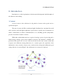


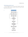


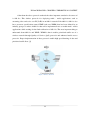
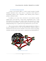

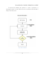

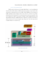

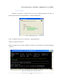
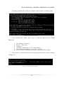
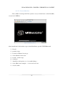


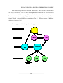


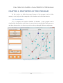

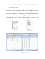

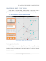
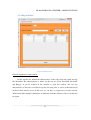


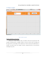
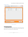

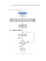


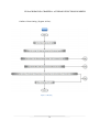


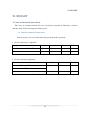
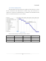

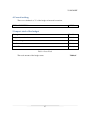


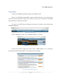

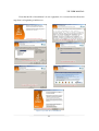


![2008 [DAMN SMALL NAS]](http://vs1.manualzilla.com/store/data/005757702_2-ad0d2f1082977ee9ed587e807bbc0127-150x150.png)