
1
AN ABSTRACT OF THE THESIS OF
Brenda E. Thompson for the degree of Master of Science in Electrical and Computer
Engineering presented on January 17, 1995. Title: Three-Dimensional Finite Element
Design Procedure for the Brush less Doubly Fed Machine.
Redacted for Privacy
Abstract approved:
Dr. Alan K. Wallace
Brush less Doubly Fed Machines (BDFM) have potential advantages in variable
speed generation and adjustable speed drive applications. The most significant of these
advantages is a reduction in the power electronic converter rating, and therefore a
reduction in overall system cost. Presently, efforts are being directed at optimizing the
design of the BDFM and investigating areas of commercial feasibility. One possible aid
in the investigation of design alternatives is finite element analysis.
Finite element analysis is a numerical method for determining the field
distribution in a dimensional model. Finite element techniques have been successfully
used for some time in the design of induction, reluctance and permanent magnet
machines. However, the characteristics of the BDFM require adjustment of the finite
element design procedure used for conventional singly-fed induction machines. In this
thesis, a three-dimensional finite element design procedure for modeling the BDFM has
been developed. This design procedure avoids the difficulties previously associated
with finite element modeling of the BDFM.
.
The three-dimensional finite element design procedure developed in this thesis
was used to model the 6/2 pole 5 horsepower BDFM laboratory machine. From the
simulation results, the induced currents in the BDFM rotor bars were calculated.
In the course of investigating three-dimensional finite element analysis for the
BDFM, two different commercially available finite element analysis software packages
were examined and tested. The first was Maxwell 3D Field Simulator produced by
Ansoft Corporation, and the second was MSC/EMAS (Electromagnetic Analysis
System) and MSC/XL by MacNeal-Schwendler Corporation. These two software
packages are compared and their advantages and disadvantages/limitations are
discussed.
A tutorial for setting up and solving a three-dimensional BDFM model using
MSC/XL and MSC/EMAS is presented. This goal of this tutorial is to guide a new user
of MSC/XL and MSC/EMAS through the creation, setup, simulation, and analysis of a
BDFM model. This tutorial contains condensed information included in the MSC/XL
and MSC/EMAS program documentation provided by MacNeal-Schwendler. In
addition, modeling techniques particular to the BDFM, which are not included in the
program documentation, are described. This tutorial is applicable only to those
individuals interested in learning how to use MSC/XL and MSC/EMAS in order to
simulate a BDFM model.
Three-Dimensional Finite Element Design Procedure for the Brush less
Doubly Fed Machine
by
Brenda E. Thompson
A THESIS
submitted to
Oregon State University
in partial fulfillment of
the requirements for the
degree of
Master of Science
Completed January 17, 1995
Commencement June 1995
Master of Science thesis of Brenda E. Thompson presented on January 17, 1995
APPROVED:
Redacted for Privacy
Major Professor, representing Electrical and Computer Engineering
Redacted for Privacy
Chair of Department of Electric 1 and Computer Engineering
Redacted for Privacy
Dean of Graduate
I understand that my thesis will become part of the permanent collection of Oregon State
University libraries. My signature below authorizes release of my thesis to any reader
upon request.
Redacted for Privacy
Brenda E. Thompson, Auth r
ACKNOWLEDGMENTS
I would like to thank my major professor, Dr. Alan Wallace, for the amount of
time and effort he has put into guiding me towards the completion of my thesis, for first
suggesting that I get involved in working with finite element analysis of the BDFM, and
for his willingness to help when I had questions about the BDFM or my finite element
results. I would also like to thank Dr. Rene Spee and Dr. G. C. Alexander for their
helpful suggestions about my finite element work and other topics. Special thanks to
Dr. Alan Wallace, Dr. Molly Shor, Dr. G. C. Alexander, and Dr. David Butler, Graduate
Council Representative, for being on my defense committee.
I would like to thank all the student members of the BDFM research and design
group for their helpful suggestions about my work, during BDFM meetings and other
times: Shibashis Bhowmik, Michael Boger, Bhanu Gorti, Tim Lewis, Sreekumar
Natarajan, Arif Salim, Ernesto Weidenbrug, and Donsheng Zhou. I would like to thank
Arif Salim for introducing me to finite element analysis and teaching me how to use
Maxwell 2D Field Simulator by Ansoft Corporation.
I would like to thank James Neuner and Pat Lamers, members of the MacnealSchwendler customer support staff, for their willingness to answer questions about
Macneal-Schwendler's software in a timely manner. Their help was very valuable in
learning how to use this software.
I would like to thank Tom Lieuallan for his help in setting up the HP
workstation, installing the finite element software, and for his willingness to provide
help whenever I had a computer question or problem.
I would like to thank Ed Lake for helping me to proofread my thesis, and for his
help instructing me in the creation of the figures contained in this thesis with AutoCad.
Finally, I would like to thank my parents and close friends for their love, support
and encouragement during my years at Oregon State University.
Table of Contents
1.
Introduction
1
2.
Brush less Doubly Fed Machine
3
3.
4.
2.1
BDFM Characteristics
3
2.2
Basic Performance Equations
4
2.3
Applications of the BDFM
6
Finite Element Analysis Method
7
3.1
Definition and Concept
7
3.2
Finite Element Model
7
3.3
Solution of Maxwell's Equations
8
3.4
Data Recovery
Finite Element Design Procedure for the BDFM
4.1
4.2
4.3
12
13
Methods of Modeling Induction Motors
13
4.1.1 Solution Frequency
13
4.1.2 Periodic Boundary Conditions
14
FE Modeling of Doubly Fed Characteristics
15
4.2.1 Complications of the Nested Rotor Structure
4.2.2 Inclusion of Two Excitation Frequencies
4.2.3 Boundary Conditions More Difficult to Determine
15
15
15
Three-Dimensional Simulation of the BDFM
16
4.3.1 Modeling in the Rotor Reference Frame vs. the Stator Reference
4.4
Frame
4.3.2 Symmetry of the BDFM Model
17
18
Results of the BDFM Model Simulations
19
Device Geometry
4.4.2 A Coarse 360 Degree BDFM Model
4.4.2.1 Materials...
4.4.2.2 Excitations
4.4.2.3 Boundary Conditions
4.4.2.4 Solution Frequency for an AC Analysis
4.4.1
4.4.2.5 Results
4.4.2.5.1 Contour Plot of Magnetic Vector Potential
4.4.2.5.2 Arrow Plot of Magnetic Flux Density
4.4.2.5.3 Currents in the Rotor Bars
4.4.3 A Coarse 180 Degree BDFM Model
4.4.3.1 Boundary Conditions
4.4.3.2 Results
4.4.3.2.1 Contour Plot of Magnetic Vector Potential
4.4.3.2.2 Arrow Plot of Magnetic Flux Density
4.4.3.2.3 Currents in the Rotor Bars
4.4.4 A Detailed 180 Degree BDFM Model
4.4.4.1 Results
4.4.4.1.1 Currents in the Rotor Bars
4.4.4.1.2 Distribution of Conduction Current Density
Within the Rotor Bars
5.
Comparison of Two Three-Dimensional Finite Element Analysis Software
Packages
5.1
Introduction
5.2 Maxwell 3D Field Simulator by Ansoft Corporation
5.2.1
5.2.2
5.3
Advantages
5.2.1.1 Solid Modeling Procedure
5.2.1.2 Step-by-Step Design Procedure
5.2.1.3 Automated Meshing Technique
Disadvantages/Limitations
5.2.2.1 Only Two Analysis Modules Available
5.2.2.2 Solution Parameters have to be Re-entered each Time a
Modification is Made
5.2.2.3 Very Poor Program Diagnostics
5.2.2.3.1 Program Continues to Execute and Status is
not Available to the User
5.2.2.4 Poor Customer Support
5.2.2.5 No results due to Problem Encountered
MSC/XL and MSC/EMAS by MacNeal-Schwendler Corporation
20
22
23
24
24
26
27
27
27
30
32
34
34
35
36
36
39
40
40
43
49
49
49
49
49
51
52
53
53
54
54
55
55
56
56
5.3.1
5.3.2
6.
A.
Advantages
5.3.1.1 Many Modeling Modules Available for a Variety of
Problems
5.3.1.2 Well Documented Program Diagnostics
5.3.1.3 Setup Parameters are Saved and only have to be
Entered Once
Disadvantages/Limitations
5.3.2.1 Wireframe Modeler
5.3.2.2 No Step-by-Step Procedure Menu
56
56
57
57
58
58
59
Conclusions and Recommendations
60
BIBLIOGRAPHY
64
APPENDIX
66
Tutorial for Setting up and Solving a 3D BDFM Model using MSC/XL and
MSC/EMAS
67
A.1
Introduction
A.2 An Overview of MSC/XL
A.2.1
Screen Layout
A.2.2 Using the Mouse
A.2.3 Capabilities
A.2.4 Data Files
67
67
68
68
70
70
A.3 An Overview of MSC/EMAS
72
A.4 Modeling Tasks
74
A.4.1 Planning the MSC Session
A.4.1.1 Deciding on Units
A.4.1.2 Drawing a symmetry "Wedge"
A.4.1.3 Entering MSC/XL
A.4.2 Creating Geometry
A.4.2.1 "Undo" Command and "Delete Item" Option
A.4.2.2 Defining a New Coordinate System
A.4.2.3 Creating Points
A.4.2.3.1 Define Point
A.4.2.4 Creating Curves
A.4.2.4.1 Connect Points
A.4.2.4.2 Sweep Point
A.4.2.4.3 Reflect Curve
75
75
76
78
79
79
80
81
81
82
82
83
84
A.4.2.4.4 Rotate Curve
A.4.2.4.5 Define Curve
A.4.2.5 Creating Surfaces
A.4.3 Generating Finite Elements
A.4.3.1 Finite Element Terminology
A.4.3.1.1 Grid Points
A.4.3.1.2 Elements
A.4.3.2 Key Factors in Meshing
A.4.3.2.1 Element Choice
A.4.3.2.2 Element Connections
A.4.3.2.3 Mesh Density
A.4.3.2.4 Mesh Order
A.4.3.2.5 Element Distortion
A.4.3.3 Preparation for Meshing - Assigning PIDs
A.4.3.4 Meshing in MSC/XL
A.4.3.4.1 Parametric Meshing
A.4.3.4.2 Connect Grids
A.4.3.4.3 Reflecting and Rotating the Mesh
A.4.3.5 Mesh Checking Procedures
A.4.3.5.1 Duplicate Grid Points
A.4.3.5.2 Unconnected Grid Points
A.4.3.5.3 Duplicate Elements
A.4.3.5.4 Free Edges or Free Faces
A.4.3.5.5 Element Voids
A.4.3.6 Mesh Organization
A.4.3.6.1 Using Groups
A.4.3.6.2 Using Parts
A.4.3.7 Extruding the Two Dimensional Mesh to Make a
Three-Dimensional Mesh
A.4.4 Problem Setup
A.4.4.1 Material Properties
A.4.4.1.1 Permittivity
A.4.4.1.1.1 Isotropic Permittivity
A.4.4.1.1.2 Anisotropic (Symmetric)
Permittivity
A.4.4.1.1.3 Unsymmetric Permittivity
A.4.4.1.2 Conductivity
A.4.4.1.3 Permeability
A.4.4.1.4 Setting Material Properties in MSC/XL
A.4.4.1.5 Material Properties for the BDFM Model
A.4.4.2 Excitations
A.4.4.2.1 Available Excitations
A.4.4.2.2 Applying Excitations to the BDFM Model
A.4.4.3 Boundary Conditions
A.4.4.3.1 Fixed Boundary Conditions
84
86
87
87
88
88
89
89
90
91
92
92
93
94
96
97
98
99
101
102
103
103
103
105
106
106
107
108
111
111
112
112
113
113
113
114
115
117
118
119
119
122
123
A.4.4.3.2 Periodic Boundary Conditions
A.4.4.3.3 Applying Boundary Conditions to the
BDFM Model
A.4.4.3.3.1 Outer Boundaries
A.4.4.3.3.2 Periodic Boundaries for the 180
Degree Model
A.4.4.4 AC Analysis Preparation
A.4.4.4.1 Control Section
A.4.4.4.2 Unit Section
A.4.4.4.3 Degrees of Freedom
A.4.5 Solving the Problem
A.4.5.1 Invoking MSC/EMAS
A.4.5.2 System Requirements
A.4.5.3 Solution Time
A.4.6 Results and Validation
A.4.6.1 Accessing MSC/EMAS Results
A.4.6.2 Producing Contour Plots
A.4.6.3 Producing Arrow Plots
A.4.6.4 Results Plots on Cut Surfaces
A.4.6.5 XY Plotting along Cut Paths
A.4.6.6 Calculations
A.4.6.7 Generating Hardcopy Files
125
126
126
127
128
129
129
129
129
129
131
132
134
134
135
136
138
139
141
142
List of Figures
2.1 BDFM Stator Structure
3
2.2 BDFM Rotor Structure
4
2.3 Velocities of Interacting Fields
5
Stator Lamination
21
4.2 Rotor Lamination
20
4.3 Coarse Three-Dimensional 360 Degree BDFM Finite Element Model
22
4.4 Stator Excitations for the 360 Degree BDFM Model
25
4.5 Boundary Conditions for the 360 degree BDFM Model
26
4.6 Contour Plot of Magnetic Vector Potential along a Center Cross-Section
of the 360 Degree BDFM Model
28
4.7 Arrow Plot of Magnetic Flux Density along a Center Cross-Section of
the 360 Degree BDFM Model
29
4.8 Rotor Bar Labels for the 360 Degree BDFM Model
32
4.9 Coarse Three-Dimensional 180 degree BDFM Finite Element Model
33
4.10 Boundary Conditions for the Coarse 180 Degree BDFM Model
35
4.11 Contour Plot of Magnetic Vector Potential along a Center Cross-Section
of the Coarse 180 Degree BDFM Model
37
4.12 Arrow Plot of Magnetic Flux Density along a Center Cross-Section of
the Coarse 180 Degree BDFM Model
38
4.13 Rotor Bar Labels for the Coarse 180 Degree BDFM Model
39
4.14 Detailed Three-Dimensional 180 degree BDFM Finite Element Model
41
4.15 Rotor Bar Labels for the Detailed 180 Degree BDFM Model
41
4.16 Slot Span vs. Rotor Bar Current Magnitude
43
4.1
4.17 Path along which Conduction Current Density was Plotted from Bottom to Top
45
4.18 Conduction Current Density in Bar 6 (in reference to Figure 4.17)
46
4.19 Conduction Current Density in Bar 7 (in reference to Figure 4.17)
46
4.20 Path along which Conduction Current Density was Plotted from Right to Left
47
4.21 Conduction Current Density in Bar 6 (in reference to Figure 4.20)
48
4.22 Conduction Current Density in Bar 7 (in reference to Figure 4.20)
48
List of Tables
4.1 Material Properties used in the 360 Degree BDFM Model
24
4.2 Total Calculated Currents in the Rotor Bars for the 360 Degree BDFM
Model
31
4.3 Total Calculated Currents in the Rotor Bars for the Coarse 180 Degree
BDFM Model
4.4 Total Calculated Currents in the Rotor Bars for the Detailed 180 Degree
BDFM Model
36
42
List of Appendix Figures
A.1 MSC/XL Screen Layout
69
A.2 Data Flow in MSC/XL
71
A.3 Data Flow in MSC/EMAS
73
A.4 Radial Cross-Section of the BDFM Model
77
A.5 Finite Elements and Grid Points
89
A.6 Available Two and Three-Dimensional Elements
91
A.7 Distortion of Midedge Nodes, Aspect Ratios, and Taper Angles
94
A.8 Typical Mesh Errors
102
A.9 Fixed Boundary Conditions
123
A.10 Alternating Periodic Boundary Conditions
125
A.11 Disk Space Requirements for MSC/EMAS based on the cellular cube and
flat plate for MSC/NASTRAN solution 101 run [17]
133
List of Appendix Tables
A.1 MKS Units
76
A.2 Assignment of PIDs to Two Dimensional Elements
95
A.3 Assignment of PIDs to Three-Dimensional Elements
95
A.4 Supplied Materials in MSC/XL
116
A.5 Materials Used in the Setup of the BDFM Model
118
A.6 Six Pole Stator Winding Layout
119
A.7 Two Pole Stator Winding Layout
120
Three-Dimensional Finite Element Design Procedure for the Brush less
Doubly Fed Machine
1. Introduction
Due to recent improvements in power electronics, adjustable speed drives
(ASDs) are being installed in increasing numbers in industrial applications. However,
the majority of all industrial and commercial motors still operate at fixed speed.
Similarly, fixed speed generators provide the bulk of the world's power supply, although
many power sources could be more efficiently converted if variable speed generation
(VSG) were used.
The transition from fixed speed systems to ASD and VSG systems has been
delayed by the fact that the speed of AC machines is linked to their frequency. Although
frequency control by power electronics has made significant advances in recent years, it
still has two major obstacles preventing its more widespread application. First, the cost
of electronic power converters is many times higher than the cost of the machines they
control. Second, the electronic power converters pollute the power supply system with
harmonics of voltage and current. Possible solutions to the harmonic problem serve to
increase the cost of the system. Therefore, it is important to investigate possible
methods for minimizing the ratings, and hence costs, of power electronic converters.
Ongoing studies at Oregon State University have shown the potential for many
advantages by using a doubly-fed connection of the self-cascaded induction machine in
ASD and VSG applications [1-5]. The use of a self-cascaded, or brushless doubly-fed
machine (BDFM), in combination with a power electronic converter, can offer a number
of advantages over conventional induction machines in ASD and VSG systems. These
advantages include tolerance to power converter failure, controllable power factor, and
2
reduced harmonic pollution. Most importantly, depending on the requirements of the
application, a reduction in the power electronic converter rating, and therefore cost, can
be achieved.
Presently, efforts are being directed at optimizing the design of the BDFM and
investigating areas of commercial feasibility. One possible aid in the investigation of
design alternatives is finite element analysis. Finite element analysis is a numerical
method for determining the field distribution in a dimensional model. This thesis will
emphasize only the electromagnetic field distribution in a three-dimensional model
geometry. Finite element techniques have been successfully used for some time in the
design of induction, reluctance and permanent magnet machines. From a finite element
solution, important design quantities such as flux distribution, flux density, winding
inductance, eddy currents, hysteresis losses, force, torque and losses can be calculated.
Applying the finite element technique to the BDFM, however, has posed a number of
difficulties. This thesis will present a design method for modeling the BDFM using
finite element techniques.
3
2. Brushless Doubly Fed Machine
2.1
BDFM Characteristics
The stator winding connection of the BDFM is based on the work of L. J. Hunt
[6] and later developments by Creedy [7]. The BDFM stator, as shown in Figure 2.1,
consists of two sets of three phase stator windings of different pole numbers and
3phase
adj. frequency
Bidirectional
Converter
(25% rating)
3phase
60 hz
0
0
fP
p
Figure 2.1: BDFM Stator Structure
different frequencies. These two separate sets of windings are wound on the same stator
frame and share the same slots. One set of windings is the power winding, which is
connected directly to the power supply system and which supplies the bulk of the
machine power. The second set is the control winding, which supplies a fraction of the
machine power through a power electronic converter. The advantage of the BDFM
system over more conventional motors and generators is that most of the power flows
directly between the machine and the power system. Therefore, the rating of the
4
required converter should be a fraction of that required to process all of the machine
power, thus reducing cost and induced harmonics of the power electronics.
The rotor design of the BDFM is based on work by Creedy and Broadway [7,8].
As shown in Figure 2.2, the BDFM rotor is an unique, cage type rotor with nested loops.
Unlike the squirrel cage rotor of an induction motor, which has rings to short all the
rotor bars on both ends, the BDFM rotor has a ring to short all the rotor bars only on one
end while at the other end the bars are selectively shorted together to form distinct
loops. The rotor design is mechanically simple enough to be die-cast, while at the same
time having the capability of supporting two fields of different pole numbers and
different frequencies from the stator.
Isolated
Endring
n
1
Common
Endring
Figure 2.2: BDFM Rotor Structure
2.2
Basic Performance Equations
The number of loop groupings or rotor nests is determined by the sum of the
pole-pairs of the power and control windings:
5
Number of Nests = Pp + Pc
(Equation 2.1)
where Pp is the number of pole-pairs of the power winding, and Pc is the number of
pole-pairs of the control winding.
The BDFM has all the robust, maintenance-free features of a squirrel-cage
induction machine. In order to operate successfully, the BDFM must switch from
operation as two induction motors in the same magnetic circuit (the "double-induction"
mode) to a mode where the rotor field induced by one of the stator windings is locked
together with the stator field of the other stator winding, and vice versa (the
"synchronous mode").
fc
PP
Pc
f RC
rotor
fr
PP
positive
direction
Figure 2.3: Velocities of Interacting Fields
In the synchronous mode the field interaction and the mechanical speed of the
rotor, as shown in Figure 2.3, are related by [9]
Dp
P
and
= f.r + fRc
p
iP
(Equation 2.2)
6
f.=
f+
fRp
Pc
(Equation 2.3)
Pc
where f., and fe are the frequencies applied to the power and control windings,
respectively; fRp and fRC are the rotor frequencies induced by interaction with the fields
of the power and control windings; fr is the mechanical rotational frequency.
For synchronous operation to be attained, it is required that
Lc =fRP
(Equation 2.4)
with the result that
.fr =
f±L
PPP + Pc
(Equation 2.5)
The control frequency, fc, can either be positive (same sequence as fp), or
negative (opposite sequence to fp). The electrical frequency of rotor currents in
synchronous operation can be related to the system frequencies as [9]
fr,ri= fp Ppfr = Pcf, T- fc
2.3
(Equation 2.6)
Applications of the BDFM
The BDFM can be used in place of commercial and industrial squirrel-cage AC
induction machines. It is particularly suited for potential niche applications in ASD or
VSG systems including, but not limited to, pump drives, wind power generation, and
automotive alternators.
7
3. Finite Element Analysis Method
3.1
Definition and Concept
Finite Element Analysis (FEA) is a numerical method that is widely used to
solve many engineering problems. One application of FEA is to solve for the
electromagnetic fields in electrical devices. Electromagnetic fields represent the
foundation of all electrical engineering. Maxwell's equations, a system of four coupled
partial differential equations, serve as the basis for electromagnetic field calculations.
The solution of these equations, however, is a very difficult task.
Often engineers approximate field behavior through abstract concepts. Much
insight can be gained from analytic techniques and approximations. However, such
techniques are useful only in relatively simple devices, and at some point
approximations will fail. More often engineers require accurate solutions involving
complicated materials, geometries, and loading conditions. For this reason, engineers
are turning to numerical methods for answers to real life problems.
FEA is one numerical method of solving Maxwell's differential equations. There
are several steps that make up the finite element method.
3.2
Finite Element Model
The first step in FEA is to specify a finite element model. The model geometry
describes the size and shape of the device to be analyzed. The geometry is divided into
8
subregions called finite elements. Elements may be irregular so that the modeling of
complicated geometries is both easier and more accurate. Points where elements join
are referred to as grid points. Material properties, excitations, and boundary conditions
are applied to the finite element model. Material properties associated with elements
represent the permittivity, conductivity, and permeability properties of the various
materials in different regions of the model. Excitations such as currents are applied to
the model. Boundary conditions are used to simulate physical behavior outside the
model boundaries.
3.3
Solution of Maxwell's Equations
Maxwell's equations are the basis for electromagnetic field calculations. These
four partial differential equations relate the space and time variation of electric and
magnetic fields to material properties, and to excitations. They describe a broad range
of behavior, including electrostatics, magnetostatics, eddy currents, waveguides,
antennas, etc. Thus, Maxwell's equations form the basis for the analysis of virtually
every electromagnetic device, from computer microcircuitry, to large power generators
and transformers. Maxwell's equations [10] are traditionally written as:
v .n
P free
(Equation 3.1)
vh=o
(Equation 3.2)
vxt,ii
(Equation 3.3)
vxii=icond F ii
(Equation 3.4)
9
These four equations state the following:
Gauss's law: the sources of D are free charge
B has no sources
Faraday's law: electric fields are induced by time-varying magnetic fields
Ampere's law: the sources of T-1 are conduction current plus the
displacement current
The fields (electric field E and magnetic field B) are the primary unknown
quantities of interest in electromagnetic field analysis. However, there are three
disadvantages to solving directly for the unknown vectors E and /3 First, the six
.
unknown components of these two fields in three-dimensional space cannot be chosen
arbitrarily because they are related through Maxwell's equations. Thus, the number of
unknowns is larger than is actually needed. The second disadvantage is related to
discontinuities in material properties. There are two well-known boundary conditions
that must be met at such interfaces: (1) the normal component of D must be
continuous across the interface; (2) the tangent component of H must be continuous.
Any solution strategy that involves E and B must enforce these conditions at every
interface. This requirement puts an unnecessary burden on numerical computations.
The third disadvantage is that E and B may be infinite at sharp corners of certain
materials. These infinite solutions cause numerical difficulties in computers.
10
Therefore, electromagnetic potential functions are introduced to eliminate the
disadvantages of dealing with E and B directly. These potential functions are the
magnetic vector potential A , and a time-integrated electric scalar potential, If . In
terms of these potential functions, the electric and magnetic fields are given by [10]:
(Equation 3.5)
t= V
tif
A
(Equation 3.6)
Maxwell's equations are rewritten in terms of these potential functions. The
values of A and 'If at the model grid points are called degrees of freedom (DOFs).
There are four DOFs at each grid point: three components of the vector potential and
one component of the scalar potential.
The principle of virtual work is now used to formulate the overall energy stored
in the solution region according to the following energy relationships:
h
(Equation 3.7)
WE = 2 E :6
(Equation 3.8)
Wif =
17/
.
The objective is to solve for the unknown potentials A and I' by minimization of the
energy function [10]. The problem volume is divided into finite elements. The energy
associated with each element is computed in terms of the potential degrees of freedom;
the results are then summed over the elements to represent the energy of the entire
problem volume. When the energy function is set to zero, a single equation is obtained.
11
This equation is entirely equivalent to Maxwell's equations in their complete and
general form. This equation is [10]:
(Equation 3.9)
[6] 04+[a] fil}+[--1 1{u}={.-7}
where the vector {u} represents the four DOFs per grid point, the matrix [6] represents
permittivity, the matrix [a] represents conductivity, the matrix
[1
represents
permeability, and {J} is an excitation vector which represents the contributions of all
model excitations.
The associated initial condition is:
[E] f/1;1= Oil
(Equation 3.10)
These matrix equations, which are equivalent to Maxwell's equations in their
complete and general form, are solved using a formal series of matrix operations for the
unknown potentials:
(Equation 3.11)
The numerical methods used to solve Equations 3.7 and 3.8 are specified by
solution sequences [10]. Each sequence represents a particular mathematical technique.
Thus, a particular application may be analyzed using several techniques, such as
magnetostatic analysis, frequency response analysis, transient analysis, or eigenvalue
analysis.
12
3.4
Data Recovery
Once a solution for the potential DOFs at each grid point have been obtained,
the fields E and h are recovered within each element. Other quantities, such as
electromagnetic energies, induced conduction currents, power losses, etc., can also be
determined.
13
4. Finite Element Design Procedure for the BDFM
Methods of Modeling Induction Motors
4.1
Finite element analysis techniques have been used successfully for some time in
the design of induction, reluctance and permanent magnet machines. Neglecting end
effects, these machines can easily be investigated using two-dimensional finite element
analysis.
In three-phase ac squirrel-cage induction motors, the rotor current distribution is
one of the main unknown quantities of interest. One goal of finite element analysis for
induction machines is to calculate the induced or eddy current distribution in the rotor
conductors, as well as the total resulting magnetic field. This can be accomplished for
an induction motor by doing an ac analysis of a two-dimensional cross-section of the
machine.
4.1.1
Solution Frequency
In an ac induction machine analysis, the frequency selected as the solution
frequency is the slip frequency, or frequency seen by the machine rotor [11]. For
example, to model the machine at start up, the solution frequency would be 60 Hz. At
high speed, a low frequency as seen by the rotor is used. The slip frequency is
appropriate to use for an ac solution because currents are induced in the rotor conductors
at the frequency seen by the rotor.
14
4.1.2
Periodic Boundary Conditions
Finite element simulations of ac induction machines, as well as other types of
electric machines, have shown that machines have an identical magnetic field
distribution on a pole by pole basis [11]. The magnetic field patterns show that only one
pole pitch needs to be modeled in a machine with identical poles. Thus, the number of
elements and grid points in a finite element model can greatly be reduced if symmetry
can be used and only one pole of the machine modeled. This is advantageous because a
model with fewer elements and grid points will have a faster solution time and require
less resources such as disk space to solve.
In an induction machine having identical poles, each pole boundary has periodic
boundary conditions. For a two-dimensional model, the periodic boundary conditions
are expressed in polar (r ,0) coordinates as [12]:
A(r ,0 0 + p) = A(r ,0 0)
(Equation 4.1)
where A is vector potential, 00 is the angle of one radial boundary, and p the pole pitch
angle. This boundary condition is called an alternating periodic boundary condition. If
the geometry requires modeling two poles, then the vector potentials on the boundary are
set equal with no negative sign. This is referred to as a repeating periodic boundary
condition. Generally, an odd number of poles requires alternating and an even number
repeating boundary conditions.
15
4.2
FE Modeling of Doubly Fed Characteristics
Applying the techniques of induction machine analysis described above to the
BDFM is difficult due to the following considerations:
4.2.1
Complications of the Nested Rotor Structure
Because of the nested loop rotor structure, (the absence of a solid endring on one
side), the BDFM analysis problem is three-dimensional in nature. The nested loops
impose electrical constraints on the model that cannot be properly represented with a
two-dimensional analysis.
4.2.2
Inclusion of Two Excitation Frequencies
The presence of two stator windings carrying currents of differing frequencies
requires the consideration of two frequencies at any time. This poses a problem because
the ac solution method requires that a single solution frequency be specified.
4.2.3
Boundary Conditions More Difficult to Determine
The symmetry of the magnetic field distribution in the BDFM is not as simple to
determine as that of an induction machine, because of the presence of the two stator
windings of different pole numbers. Thus, determining the section of the BDFM that
should be modeled to properly represent the entire machine, and the selection of the
appropriate boundary conditions, requires some consideration.
16
This chapter discusses how these difficulties have been dealt with and a finite
element procedure for modeling the BDFM has been developed.
4.3
Three-Dimensional Simulation of the BDFM
Because the BDFM analysis problem is three-dimensional in nature, three-
dimensional finite element modeling of the BDFM has been investigated. A threedimensional analysis avoids the approximations involved in developing and/or
combining two-dimensional models, and allows accurate representation of the nested
rotor structure. For this three-dimensional analysis, a commercial software package
produced by MacNeal-Schwendler Corporation (MSC), called MSC/XL and
MSC/EMAS (Electromagnetic Analysis System) was used. The work was done on a
Hewlett Packard workstation, model 715/50, with 48 MB of RAM and approximately
2.5 GB of hard disk space.
Several three-dimensional BDFM models will be presented, along with the
materials, excitations, and boundary conditions used in the setup of the models. The
results of these BDFM model simulations will also be presented. Each of the BDFM
models presented is based on the prototype 5 hp laboratory machine, which has a 6 pole
power winding and a 2 pole control winding configuration. Analysis techniques used to
model BDFM will also be discussed.
17
4.3.1
Modeling in the Rotor Reference Frame vs. the Stator Reference Frame
In finite element simulation of ac induction machines, the solution frequency
used in an ac analysis is the frequency seen by the rotor, or the slip frequency. The
frequency seen by the rotor is not as simple to imagine for the BDFM, because of the
presence of two sets of stator windings operating at different frequencies.
A way of obtaining the frequency observed by the BDFM rotor for use as the
solution frequency for an ac analysis is to model the BDFM in the rotor reference frame.
The rotor reference frame frequency, or frequency of the rotor currents during
synchronous operation of the machine, is determined from Equations 2.5 and 2.6, which
are restated here:
f -±f
fr= Pp+ Pc
(Equation 4.2)
.1;4= fp Ppf, = Pcf,
(Equation 4.3)
Equation 4.3 determines the frequency seen by the BDFM rotor during
synchronous operation. Since during synchronous operation the fields induced in the
rotor by the power and the control windings are locked together at the same frequency,
only this one rotor frequency needs to be specified in the ac analysis. If it is desired to
determine the induced rotor currents during synchronous operation of the machine,
Equation 4.3 can be used to determine the solution frequency to be used in an ac
analysis. Thus, modeling the BDFM in the rotor reference frame eliminates the need for
two frequencies to be included in the simulation at once.
18
If it is desired to model the BDFM during startup, or during other conditions
when it is not operating in synchronous mode, the fields induced in the rotor would not
be locked together at one frequency. Therefore, it is not be possible to simulate the
BDFM under dynamic conditions with the ac analysis module, because the ac solution
method requires that a single solution frequency be specified. Possibilities exist to
overcome this difficulty by using the transient analysis module, which allows waveforms
of different types and/or frequencies to be included in the analysis simultaneously.
4.3.2
Symmetry of the BDFM Model
In induction machine analysis, it has been shown that only one pole pitch of the
machine needs to be modeled because of the symmetry of the magnetic field distribution
by pole pitch. The magnetic field symmetry of the BDFM model is not as simple to
determine because of the presence of two stator windings of different pole numbers.
The finite element model of the BDFM presented in this thesis is based on the 5
horsepower BDFM laboratory machine. The laboratory machine has a 6 pole power
winding and 2 pole control winding configuration.
Theoretically, the alternating periodic boundary conditions used to model
induction machines should be appropriate for a 180 degree model of a 6/2 pole BDFM.
This is because one pole of the two-pole winding and three poles of the six-pole winding
are present in a 180 degree model. Therefore, an odd number of poles is modeled for
both windings. Since alternating periodic boundary conditions are required for an odd
number of poles, theoretically alternating periodic boundary conditions should be the
19
appropriate boundary conditions for a 6/2 pole 180 degree BDFM model. Results of the
BDFM model simulations presented in this chapter verify this idea.
The MSC/EMAS Modeling Guide [13] suggests that the best way to determine
the correct boundary conditions is to make a coarse finite element model of the entire
device and observe the relationship obeyed by the vector potential A at grid points one
pole pitch, or other distance, apart. Then these constraints are applied to a fine finite
element model of that portion of the device.
4.4
Results of BDFM Model Simulations
Several three-dimensional BDFM models were constructed and analyzed using
MSC/EMAS. First, results from a coarse 360 degree model of the BDFM are presented.
Next, results from a 180 degree model, with a finite element mesh identical to the 360
degree model, and with alternating periodic boundary conditions applied along the
symmetry plane, are presented. Comparison of the full model and half model results
verifies that the alternating periodic boundary conditions are correct. Finally, results
from a more detailed 180 degree BDFM model are presented. For each analysis,
synchronous operation of the BDFM is assumed and the ac analysis module is used. It
should be noted that the ac analysis module is a linear analysis module that does not take
into account the B - H curve of magnetic materials.
20
4.4.1
Device Geometry
Each of the three-dimensional finite element BDFM models was based on the 5
horsepower laboratory machine. The dimensions of the laboratory machine stator
laminations are shown in Figure 4.1 (shown on the following page). The stator windings
consist of a 6 pole power winding and a 2 pole control winding. The stator contains 36
slots and the stator stack length is 100 mm.
The dimensions of the laboratory machine rotor laminations are shown in Figure
4.2. The rotor laminations were custom made to provide an air gap of 0.7 mm. The
rotor was designed with 40 slots. For the 6/2 pole BDFM, the required 4 nests have 5
loops each, and no common cage.
All measurements
are in millimeters (mm)
Figure 4.2: Rotor Lamination
10.16
6.86
22.82
1 08
3.1
Slot Detail
Stator Lamination (1/2 Size)
Figure 4.1: Stator Lamination
22
4.4.2 A Coarse 360 Degree BDFM Model
A coarse 360 degree three-dimensional finite element model of the BDFM was
constructed. The main goal in construction of this model was to determine if magnetic
field symmetry exists within the BDFM and to verify what portion of the device can be
modeled using appropriate boundary conditions to accurately represent the whole
machine.
The 360 degree model had a rather coarse finite element mesh consisting of
7776 hexahedron and pentahedron elements and 8325 grid points. The finite element
model is shown in Figure 4.3.
Figure 4.3: Coarse Three-Dimensional 360 Degree BDFM Finite Element Model
23
In constructing the 360 degree model of the BDFM, a simplifying assumption
was made about the laboratory machine rotor. The rotor was modeled with only 16 slots
(instead of the actual 40 slots) and only the first and third loops of each nest were
modeled, or two loops for each of the 4 nests (instead of the actual five loops for each of
the 4 nests). This simplification was made in order to reduce the complexity of the finite
element mesh, and hence reduce the amount of disk space required to generate a
solution.
The body of the machine was modeled with two layers of three-dimensional
elements, each 50 mm long, as shown in Figure 4.3. The nested loops of the rotor, as
well as the common endring, are modeled with one layer of three-dimensional elements
extending 6.76 mm beyond the machine body on opposite sides. Ideally, several more
layers of elements should be used to obtain a more accurate representation of the
machine. The configuration described was used because of disk space limitations.
4.4.2.1
Materials
Table 4.1 lists the material properties that were assigned to the objects that make
up the BDFM model.
Note that although the stator slot actually contain copper windings, they are
modeled as air since a current density excitation is used to specify the exact current
flowing in the windings. To model the stator windings as copper would cause the
program to induce additional eddy currents in the stator windings.
24
Material
Relative
Permeability
Relative
Permittivity
Electrical
Conductivity
(siemens/meter)
Shaft
Rotor
Rotor Bars
Air Gap
6 pole Stator Slot
2 pole Stator Slot
Stator
Nested Loops
End Ring
Air
Lam. Steel
Copper
Air
Air
Air
Lam. Steel
Copper
Copper
1
1
0
2000
1
0
1
1
5.8E+07
1
1
1
1
1
1
2000
1
1
1
1
1
0
0
0
0
5.8E+07
5.8E+07
Table 4.1: Material Properties used in the 360 Degree BDFM Model
4.4.2.2
Excitations
For the 360 degree BDFM model, an equivalent surface current density is used to
establish a current flow of 100 amp-turns peak in each of the 6 pole and 2 pole slots.
Figure 4.4 shows the 6 pole and 2 pole stator winding excitation locations and directions
and specified for use in the ac analysis.
In Figure 4.4, for the 6 pole winding, Phasea = 0° , Phase,, = 240° , and
Phase, = 120° . For the 2 pole winding, Phasea = 0° , Phaseb = 120°, and
Phase, = 240° .
4.4.2.3
Boundary Conditions
Figure 4.5 shows the applied boundary conditions for the 360 degree BDFM
model. A cylindrical coordinate system is used to define boundary directions. Along
25
6 pole Stator winding
2 pole Stator winding
Figure 4.4: Stator Excitations for the 360 Degree BDFM Model
the outer radius of the model, the tangential components of the magnetic vector potential
A are set to zero (43, As). The tangential components of A are also set to zero along
the motor ends (A 4) . Setting the tangential components of A to zero along the outer
boundaries of the machine constrains the magnetic fields to remain within the machine
outer boundaries.
s
,is
1
4
I-L00
I
1
*
°
60%
1
,
S
Insalt
11,,,\LILL
1\
L
.....
_10111111n1/0/// p
.**0
itsallfilW11111
P P -441;-1
e
-.0
ifo
4S''s4/vrtlp:
iv=-/I'Vrp
owl pm /Ulla
ainowur sio
"
*7r
.'111111.64
00,
111111111
/4,111,1,1,11itit%"
as
.1
1
27
reference frame frequency of 30 Hz, which was specified as the solution frequency in the
ac analysis. This corresponds to a machine speed of 600 rpm.
In the examination of the results that follow, the reader should note that the stator
solution is in the rotor reference frame.
4.4.2.5
Results
4.4.2.5.1 Contour Plot of Magnetic Vector Potential
A contour plot of magnetic vector potential, ;I, along a cross-section of the
BDFM located at the machine center is shown in Figure 4.6.
A line of constant magnitude of vector potential A is called a magnetic flux
line. Observing the pattern of the magnetic flux lines along a planar cross section of the
machine shows the symmetry present in the machine's magnetic field distribution.
Figure 4.6 shows that the BDFM exhibits 180 degree symmetry.
4.4.2.5.2 Arrow Plot of Magnetic Flux Density
An arrow plot of magnetic flux density, B, along a cross-section of the BDFM
located at the machine center is shown in Figure 4.7.
An arrow plot of magnetic flux density represents the direction and magnitude of
the magnetic flux density with colored arrows. The colors of the arrows indicate the
magnitude of the magnetic flux density, in tesla, at every location along the machine
cross-section. This allows the user to identify areas where the machine may be
IIIINIINMIMIMIMMEIIIIIIIINE
3.1e-07
1 0.00109
0_00109 0_00218
.0021.6
0.00321
0.00327
0.00437
0.00437 - 0.00546
0.00655
0.00546
,111
0 A011
\\
i
..wos,
Uu,,.)
0.00982
0.00982
0.01092
111,,
0000104/11/11
0
,
iiiii
/0
Niliiii
W63'
ii
2t
tk#10.1744Ei
oll
inalv\\
lLtii
jai
1: ResultsCalculator
FrequencyResponse Analysis
MagneticVectorPotential FullVector
GridResults FullVector
TypeOfData Magnitude
Subcase 1
Frequency 30
Figure 4.6: Contour Plot of Magnetic Vector Potential along a Center Cross-Section of the 360 Degree BDFM Model
INIMIENIMINIMI111
5.9e-05 - 0.03582
0.07158
1 0.03582
MMOMOMMUMM
0.32192
0.28616
0.35769
0.32192
11111111111111=11
0.17887 0.07158 - 0.10735 0.14311
0.21464
0.17887
0.10735
0.14311
,
\*
lit
I I
VotliIre
ii
1
0
,
I
IOW/
.%44/11motio,442 .:
*....,%.,..4.\%11:-1-43410111'1.111111731111f1.7....;,:
,. s
alls.-406-4:,.,:1:
1
1: ResultsCalculator
equencyResponse Analysis
MagneticVectorPotential FullVector
MagneticFlunDensity FullVector
TypeOfData Real
Subcase 1
Frequency 30
Figure 4.7: Arrow Plot of Magnetic Flux Density along a Center Cross-Section of the 360 Degree BDFM Model
30
saturating. The flux density values for this BDFM model (0.35925 tesla maximum)
show that the machine is not saturating, for the previously specified excitation level of
100 amp/turns peak per slot.
An arrow plot of magnetic flux density can also be used to observe the field
symmetry pattern of the machine. The arrow plot of Figure 4.7 also shows that the field
pattern exhibits 180 degree symmetry, giving credibility to this approach.
4.4.2.5.3 Currents in the Rotor Bars
The currents flowing in every rotor bar of the BDFM rotor were determined
using MSC/XL's solution calculator. The currents were calculated by specifying a plane
perpendicular to the rotor bar direction (the xy plane) and intersecting this plane with
one rotor bar at a time. The program then calculates the total current flowing in the rotor
bar in the positive z-direction from the conduction current density by the following
formula:
I = f(i, ds)
(Equation 4.4)
where J, is the conduction current density and ds is the integration surface.
The currents were calculated at several axial (z) positions along each rotor bar,
and identical results were obtained. The calculated total currents in each rotor bar are
presented in Table 4.2, and the rotor bar labels are identified in Figure 4.8.
Table 4.2 shows that the rotor bars currents are equal in magnitude and 180
degree out of phase for rotor bars connected by a loop. In other words, the rotor currents
31
Bar Number
1
2
3
4
5
6
7
8
9
10
11
12
13
14
15
16
Real, Imaginary
Magnitude, Phase
(Amperes)
8.26766, 25.5532
-133.203, -33.6687
30.8736, -186.89
-7.13813, -87.3815
7.13833, 87.385
-30.8734, 186.89
-133.272, -33.6829
8.28426, 25.5654
-8.28503, -25.565
133.271,33.6827
-30.7961, 186.89
7.18307, 87.3974
-7.18318, -87.3998
30.796, 186.889
133.203, 33.668
-8.6676, -25.5533
(Amperes, Degrees)
26.8574, 72.0712
137.392, -165.815
189.423, -80.6197
87.6725, -94.6701
87.676, 85.33
189.423, 99.3803
137.463, -165.816
26.8741, 72.0455
26.874, -107.956
137.461, 14.1839
189.41, 99.3572
87.6921, 85.3015
87.6945, -94.6984
189.409, -80.6428
137.393, 14.1851
26.8572, -107.927
Table 4.2: Total Calculated Currents in the Rotor Bars for the 360 Degree BDFM
Model
are equal in magnitude but flowing in opposite directions for connected bars, as is
expected. Also, the magnitude of the rotor bar currents in the first loop are greater than
the currents in the third loop, as is expected by consideration of the laboratory machine.
Thus, the rotor bar currents indicate that the BDFM model has 180 degree symmetry.
32
4.4.3 A Coarse 180 Degree BDFM Model
A three-dimensional 180 degree model of the BDFM, with a finite element mesh
identical to the 360 degree BDFM model, was set up. The material properties,
excitations, and outer boundary conditions were identical to those used for the 360
degree model. An ac solution was generated at a rotor reference frame frequency of 30
Hz, as in the 360 degree model. Alternating periodic boundary conditions were used
Bar 4
Bar 5
4,A.
Bar 3
Bart
Bar 7
'`71-4,-eAd
-::::::
040
.
so
'ts
rit
Bar 16
ho*
s.
411"*Tt
.,4.
Bar 2
Bar 6
trist,--0144,;
ii 41.14.$7
4,1010
.1
A.:11145,00.
ov,
is4..
0
Bar 15
Bar 8
13tAtitut
..Nr.
.-...itamarik..+A.
Bar 14
Bar 13
_::-...
-
Bar 9
Bar 10
,.,....
Bar 12
Bar 11
Figure 4.8: Rotor Bars Labels for the 360 Degree BDFM Model
33
along the symmetry plane of the 180 degree model. The 180 degree finite element
model is shown in Figure 4.9.
This 180 degree model had a finite element mesh consisting of 3888 hexahedron
and pentahedron elements and 4280 grid points (basically half the number of elements
and grid points utilized in the coarse 360 degree model).
Figure 4.9: Coarse Three-Dimensional 180 degree BDFM Finite Element Model
The purpose of this coarse 180 degree model simulation was to verify that the
use of alternating periodic boundary conditions on a 180 degree BDFM model produces
results consistent with those obtained for a 360 degree model.
34
4.4.3.1
Boundary Conditions
Figure 4.10 shows the applied boundary conditions for the 180 degree BDFM
model. A cylindrical coordinate system is used to define the boundary directions. The
tangential components of the magnetic vector potential, )1 , are set to zero along the
outer radius of the model and along the motor ends, as in the 360 degree model.
Alternating periodic boundary conditions were applied along the two radial faces of the
symmetry plane, at 0 = 0 and 0 = 180 degrees. This boundary condition forces every
degree of freedom (three A components and 1' ) to be equal in magnitude but opposite
in direction as follows:
Ar(r,0 0 + p,z)= Ar(r ,0 0,z)
(Equation 4.5)
4 (r,00 + p, z) = -4 (r,00,z)
(Equation 4.6)
Az(r,0 0 + p,z)= AZ (r,0 0,z)
(Equation 4.7)
T(r,00 +p,z) = T(r,00,z)
(Equation 4.8)
where ;1 is vector potential, 00 is the angle of one radial boundary, and p the pole pitch
angle.
4.4.3.2
Results
Examination of the results obtained from the coarse 180 degree BDFM model are
in close agreement with the results obtained from the 360 degree model, verifying the
symmetry of the BDFM model and the use of alternating periodic boundary conditions.
35
(A.,Az =0)
(AA. =0)
:,..:)::,,41:,
\**ttalrie/
v `
kr
es.\..
2.$..
'
4,140-4140/11..
*,
*--.%
...":
\;,`,40,.....40,t
'11111a0tit*
..,:"Ant
Ir.44#
1r
--,,,*
----
.,-----.40
"4144411:i-TaiTa.-40°
takimili:wmp
I(r,180°,z)= -A(r,0°,z)
4-1(r,1 80° , z) = -W(r,0°,z)
0 = Cf
le
(AA, =0)
Figure 4.10: Boundary Conditions for the Coarse 180 Degree BDFM Model
4.4.3.2.1 Contour Plot of Magnetic Vector Potential
A contour plot of magnetic vector potential, A , along a cross-section of the
BDFM located at the machine center is shown in Figure 4.11.
This contour plot of magnetic vector potential is identical to Figure 4.6, the
contour plot of magnetic vector potential for the 360 degree model. This contour plot is
one verification that the alternating periodic boundary conditions are correct.
36
4.4.3.2.2 Arrow Plot of Magnetic Flux Density
An arrow plot of magnetic flux density, B, along a cross-section of the BDFM
located at the machine center is shown in Figure 4.12.
This arrow plot of magnetic flux density is almost exactly identical to Figure 4.7,
the arrow plot of magnetic flux density for the 360 degree model. This arrow plot is
another verification that the selected alternating periodic boundary conditions are
correct.
4.4.3.2.3 Currents in the Rotor Bars
The total current flowing in each rotor bar of the 180 degree model was
calculated using the same method used for the 360 degree model.
The currents were again calculated at several axial (z) positions along each rotor
bar, and identical results were obtained. The calculated total currents in each rotor bar
are presented in Table 4.3, and the rotor bar labels are identified in Figure 4.13.
Bar Number
1
2
3
4
5
6
7
8
Real, Imaginary
Magnitude, Phase
(Amperes)
8.29692, 25.0857
-132.462, -33.4865
30.8917, -186.883
-7.13535, -87.3859
7.13555, 87.3894
-30.8915, 186.883
-132.463, -33.4866
8.29609, 25.0859
Amperes, Degrees)
26.4222, 71.6987
136.629, -165.813
189.419, -80.6139
87.6767, -94.668
87.6802, 85.332
189.419, 99.386
136.63, -165.813
26.4221, 71.7006
Table 4.3: Total Calculated Currents in the Rotor Bars for the Coarse 180 Degree
BDFM Model
1111111111111111.1/
1
2.4e-07
0.00109
0.00109 - 0.00219
0.00219
0.00328
0.00328
0.00437
0.00437 - 0.00547
0.00656
0.00547
MMOMMMMOMM
0.00984
0.00875
0.80984
0.01093
RT 1: ResultsCalculator
FrequencyResponse Analysis
MagneticVectorPotential FullVector
GridResults FullVector
TypeOfData Magnitude
Subcase 1
Frequency 30
Figure 4.11: Contour Plot of Magnetic Vector Potential along a Center Cross-Section of the Coarse 180 Degree BDFM Model
-1.0e-15
1 0.03585
0.03585
0.07170
DX
1
4.07170 0.10755
0.10755
0.14340
OMMIIMMOMME
0.14340
0.17924
0.17924
0.21509
9
0.32264
0.35849
RT 1: ResultsCalculator
FrequencyResponse Analysis
MagneticVectorPotential FullVector
MagneticFluxDensity FullVector
TypeOfData Real
Subcase 1
Frequency 30
Figure 4.12: Arrow Plot of Magnetic Flux Density along a Center Cross-Section of the Coarse 180 Degree BDFM Model
39
Bar 4
Figure 4.13: Rotor Bars Labels for the Coarse 180 Degree BDFM Model
These total currents calculated for the 180 degree model agree within about 2 %
with the total currents calculated for the 360 degree model. The 2 % error may be due in
part to limitations within MSC/XL for applying the boundary conditions, that do not
allow the boundary conditions to be applied such that the 360 degree model is exactly
represented. Since the currents are in close agreement, the alternating periodic boundary
conditions are verified.
4.4.4 A Detailed 180 Degree BDFM Model
A finer and more detailed 180 degree model of the BDFM was constructed. The
goal of constructing this model was to obtain a more accurate representation of the 5
horsepower BDFM laboratory machine.
40
This detailed model included all 40 of the rotor bars present in the laboratory
machine, as well as all 5 of the loops per each of the 4 nests. A finer finite element mesh
was used, especially in the rotor conductors and the air gap, where field gradients change
most rapidly. The finite element mesh consisted of 8976 hexahedron and pentahedron
elements and 9510 grid points. The finite element model is shown in Figure 4.14.
The body of the machine was modeled with two layers of three-dimensional
elements, each 50 mm long, as shown in Figure 4.14. The nested loops of the rotor, as
well as the common endring, are modeled with one layer of three-dimensional elements
extending 6.76 mm beyond the machine body on opposite sides.
Identical excitations and boundary conditions, and similar material properties to
those used in the coarse 180 degree BDFM model were used in for the setup of this
detailed 180 degree model. An ac solution was generated, again using a rotor reference
frame frequency of 30 Hz.
4.4.4.1
Results
4.4.4.1.1 Currents in the Rotor Bars
The total current flowing in each rotor bar of the detailed 180 degree model was
calculated using the same method discussed previously.
The currents were again calculated at several axial (z) positions along each rotor
bar, and identical results were obtained. The calculated total currents in each rotor bar
are presented in Table 4.4, and the rotor bar labels are identified in Figure 4.15.
ar \
A940
IIIP°17
......,,01%
-
-
-
.
..
\.
.
,
...-0.=.1
.:
\
V
/O 00
'0*
-.ow=
17:0
...i
_......,
MVO
..---- ...---
A
.....:---
......
k.0-,---------00-_,....._,
/voamMI :7-41/
thnomiliza =
liOr
;'
Seitilj
\
4
41=4
lb
\\
41' 14 +
*_
N.
"*
1
\\
s
\Ile
A\t
4\
\
\
,
.
\
... N
I \i.
IL 1L,
# ii, 1
,
\ .k".
A
-..
Opror="--
aim Aloft
Amor left
saw 4ftv
.
%
ItsION'vz
.
.
...:
.
..
44%
UJj
W
"
4
4
ow. Avow
,
..:
is
-mutul
1011110111111111
s*****
\
42
The rotor bar currents are equal in magnitude and 180 degrees out of phase for
rotor bars connected by a loop.
The magnitude of the rotor bar currents becomes greater as the slot span of the
loops becomes larger (moving from the inner to outer loops). Figure 4.16 is a graph of
slot span vs. rotor bar current magnitude, which shows that the current magnitude
increases from the inner to outer loops.
Bar Number
1
2
3
4
5
6
7
8
9
10
11
12
13
14
15
16
17
18
19
20
Real, Imaginary
Magnitude, Phase
(Amperes)
0.0271658, -0.372618
3.10542, 0.175448
11.1839, 12.7192
-16.7531, 21.1527
115.5, -40.2878
30.2753, -140.761
-8.09887, -75.7353
-8.56011,-39.4474
1.19354, -28.9307
-4.10281,-3.87263
4.10331, 3.86986
-1.19341, 28.932
-1.19341, 39.4493
8.09896, 75.7372
-30.2749, 140.76
-115.502, -40.2885
-16.7533, 21.1523
11.1836, 12.7189
3.10525, 0.175529
0.0270078, -0.372556
(Amperes, Degrees)
0.373607, -85.8302
3.11038, 3.23362
16.9368, 48.675
26.9833, 128.379
122.325, -160.771
143.98, -77.8615
76.1671, -96.1038
40.3655, -102.243
28.9553, -87.6376
5.64184, -136.653
5.6403, 43.3229
28.9566, 92.362
40.3674, 77.7569
76.169, 83.8963
142.979, 102.138
122.326, -160.771
26.9832, 128.38
16.9364. 48.6752
3.1102, 3.23529
0.373534, -85.8537
Table 4.4: Total Calculated Currents in the Rotor Bars for the Detailed 180 Degree
BDFM Model
Information of this type, on slot span vs. rotor bar current magnitude for the
range of operating frequencies, should be used to design a more effective rotor for the
43
BDFM. A grading of bar size within the loops of each nest, with the outer loops having
the largest conductor size, should be investigated as a possible means of equalizing or
improving current distribution within the loops, or equalizing loss distribution to
minimize thermal problems.
4.4.4.1.2 Distribution of Conduction Current Density Within the Rotor
Bars
Distribution of conduction current density within each rotor bars was also
examined for the detailed 180 degree model. Plots of conduction current density across
each rotor bar from bottom to top and also from right to left were made in order to
observe how the current is distributed within the rotor bars.
Slot Span vs. Rotor Bar Current Magnitude
160
140
120
100
80
60
40
20
0
0
20
40
60
80
Slot Span (Degrees)
Figure 4.16: Slot Span vs. Rotor Bar Current Magnitude
100
44
Figure 4.17 shows the path along which the conduction current density was
plotted from bottom to top. Figure 4.18 is a plot of conduction current density in bar 6
along the path indicated in Figure 4.17. Figure 4.19 is a plot of conduction current
density in bar 7 along the path indicated in Figure 4.17.
These figures show that the conduction current density varies across the rotor
bars from bottom to top, but this variation is not great.
Figure 4.20 shows the path along which the conduction current density was
plotted from right to left. Figure 4.21 is a plot of conduction current density in bar 6
along the path indicated in Figure 4.20. Figure 4.22 is a plot of conduction current
density in bar 7 along the path indicated in Figure 4.20.
These figures show the conduction current density varies across the rotor bars
from right to left. This variation is greater than the variation observed from bottom to
top. This variation is due probably to the magnetic field distribution surrounding the
rotor bars, but is not of a sufficient magnitude to cause concern.
Figure 4.17: Path along which Conduction Current Density was Plotted from Bottom to Top
46
Conduction Current Density
E-06
4.22
4.21
E
4.2
<
4.19
p
4.18
ao
4.17
to
t
0
4.16
4.15
4.14
4.13
1
2
3
4
5
6
7
Distance across Rotor Bar 6 (mm)
Figure 4.18: Conduction Current Density in Bar 6 (in reference to Figure 4.17)
Conduction Current Density
E-06
2.24
E
cr
<
(-.1-)
2.23
2.22
0
t
2.21
V
2.2
0
0
2.19
2.18
0
1
2
3
4
5
6
7
Distance across Rotor Bar 7 (mm)
Figure 4.19: Conduction Current Density in Bar 7 (in reference to Figure 4.17)
Figure 4.20: Path along which Conduction Current Density was Plotted from Right to Left
48
Conduction Current Density
Distance across Rotor Bar 6 (mm)
Figure 4.21: Conduction Current Density in Bar 6 (in reference to Figure 4.20)
Conduction Current Density
0
1
2
3
4
5
6
7
Distance across Rotor Bar 7 (mm)
Figure 4.22: Conduction Current Density in Bar 7 (in reference to Figure 4.20)
49
5. Comparison of Two Three-Dimensional Finite Element Analysis Software
Packages
Introduction
5.1
In the course of investigating three-dimensional finite element analysis for the
BDFM, two different commercially available finite element analysis software packages
were examined and tested. The first was Maxwell 3D Field Simulator produced by
Ansoft Corporation [14], and the second was MSC/EMAS (Electromagnetic Analysis
System) [10] and MSC/XL [15] by MacNeal-Schwendler Corporation (MSC). This
chapter will compare these two software packages and discuss their advantages and
disadvantages/limitations.
5.2
Maxwell 3D Field Simulator by Ansoft Corporation
5.2.1
Advantages
The main advantages of Maxwell 3D Field Simulator by Ansoft Corporation are
its solid modeling procedure, step-by-step design process, and automated meshing
technique.
5.2.1.1
Solid Modeling Procedure
In a solid modeler, the finite element model is defined by the device structure or
geometry, which consists of a group of "solid" objects. Throughout the modeling
50
process, the solid objects that define the model are manipulated by referring to their
names. For example, as the device structure or geometry is being created, solid objects
such as cylinders, blocks, spheres, etc., are each assigned a name. Objects can then be
rotated, copied, displayed or removed from the display, and have material properties
assigned to them by referring to their names. This is a very convenient and easy way of
manipulating the device geometry.
The main advantage of a solid modeling procedure is that the finite element
model is defined by its geometry, a set of solid objects, and not by the finite element
mesh itself. This allows the mesh to be easily modified if necessary, without having to
redefine that entire model. The mesh can be refined throughout the model, or only in a
particular object by specifying the object name.
The solid modeling procedure is one major advantage that Maxwell 3D Field
Simulator has over MSC/XL. MSC/XL uses a wireframe modeling procedure, in which
the finite element model is defined by the actual finite elements and grid points. A
wireframe modeler is more difficult to use than a solid modeler. A wireframe model is
manipulated by referring to collections of finite elements that make up the geometry.
Therefore, the user must keep track of which element identification numbers belong to
what part of the geometry. If the model is large, this can be quite a task. Also, in a
wireframe modeler, once the finite element model is completed, it is not possible to
change or refine the mesh without creating the whole model over again, which requires a
substantial investment of time.
51
With Maxwell 3D Field Simulator's solid modeling procedure, analysis results
can be calculated and displayed for a particular object by selecting its name. The solid
modeling procedure makes creation, viewing, refinement of the mesh, and results
analysis easy for the user.
5.2.1.2
Step-by-Step Design Procedure
Maxwell 3D Field Simulator uses a step-by-step design procedure, which makes
the program easy for users unfamiliar with finite element analysis to learn and use.
When the program is started, the Maxwell 3D Field Simulator main menu appears,
listing the general procedure steps for the user to follow. These general procedure steps
are [14]:
Select Solver Type
Draw Geometric Model
Setup Materials
Setup Boundary Conditions
Setup Executive Parameters
Setup Solution Parameters
Solve
View Fields
The program displays a check mark next to each step after it has been successfully
completed. In general, the steps must be chosen in the sequence listed above. For
example, the "Setup Materials" step is operable only after a geometric model has been
52
created using the "Draw Geometric Model" step. This step-by-step procedure is helpful
for new users because it makes sure that each design step is completed, and in the
appropriate order.
5.2.1.3
Automated Meshing Technique
The Maxwell 3D Field Simulator uses an automated meshing technique. The
program automatically generates an initial finite element mesh when "Setup Materials"
is chosen from the main menu. If desired, the user has the option of refining the mesh in
selected areas once the initial mesh in complete, by choosing the object to be refined.
The program then automatically adds a specified number of additional elements to the
selected object.
The automated meshing procedure used by Maxwell 3D Field Simulator has the
advantage of being faster and much easier to use than a manual meshing technique, such
as the one used by MSC/XL. Manual meshing is slow and requires a lot of attention
from the user, as it is prone to user errors. An automatic meshing procedure is very
helpful for users unfamiliar with finite element analysis, who may not know how to
design an effective finite element mesh.
The automated meshing procedure used by Maxwell 3D Field Simulator does not
give the user control over the exact size, shape, and position of each individual element,
as the manual meshing technique used by MSC/XL does. However, this type of user
control is probably not necessary. Automated meshing is faster, much easier for the
53
user, and reduces the chance of user error. An automated meshing technique is
definitely a benefit for new users.
5.2.2
Disadvantages/Limitations
5.2.2.1
Only Two Analysis Modules Available
At the time of this evaluation, Maxwell 3D Field Simulator included only two
analysis modules (or solution methods) that were available as full releases. These were
the Electrostat module and the Magnetostat module. The Electrostat module is used to
compute static electric fields due to voltage distributions and charges. It has no use for
the BDFM analysis problem. The Magnetostat module is used to compute static
magnetic fields, due to DC currents, static external magnetic fields, and permanent
magnets. It has some use for the BDFM problem if the rotor bar currents are already
known from lab data and the magnetic field distribution and magnitude needs to be
calculated. It cannot be used to calculate induced currents in the rotor conductors, one of
the main quantities of interest in the BDFM analysis problem.
The Maxwell 3D Field Simulator analysis module that was used predominately
was the Eddy Current module. This module can be used to calculate time-varying
magnetic fields due to AC currents and oscillating external magnetic fields. It should be
used for the BDFM problem to calculate currents induced in the rotor bars by the AC
three-phase stator windings. However, at the time of evaluation, the Eddy Current
54
Module was still a "beta test version", which can explain the many glitches and
problems that were encountered in working with it.
5.2.2.2
Solution Parameters have to be Re-entered each Time a
Modification is Made
In the setup procedure used by Maxwell 3D Field Simulator, all of the material
property and excitation setup parameters for the entire model have to be re-entered each
time any modification is made. Likewise, each time a modification is made to the model
boundary conditions, all of the boundary conditions must be re-entered. In finite
element modeling, it is often informative to observe the effect of changing one model
property at a time. For example, the material property of one object in the model may be
changed, the magnitude of the excitations may be varied, or a particular boundary
condition may be changed. Having to re-enter all of the material properties and
excitations or re-enter every boundary condition each time a small modification is made
is not very convenient.
5.2.2.3
Very Poor Program Diagnostics
The main problem with Maxwell 3D Field Simulator was its very poor program
diagnostics. No error messages are provided by the program to help the user identify
problems during the solution process.
55
5.2.2.3.1 Program Continues to Execute and Status is not Available to the
User
While Maxwell 3D Field Simulator was solving a finite element problem, the
program would continue to execute without issuing error or information messages. The
only information provided to the user about the solution status was a shaded bar, ranging
from 0 to 100 percent, that would appear on the screen supposedly to allow the user to
monitor the progress of the system in completing the solution. This presented the
problem that sometimes the program would continue to "solve", sometimes for over one
week, with the shaded bar still at 0 percent and no other information available. The
program did not display any error or information messages (such as disk full, more swap
space needed, more memory needed, etc.) to let the user know what was happening or
what problems had been encountered. The user was unaware whether to continue to let
the program solve, or to choose to terminate and make modifications.
Occasionally, the solution process would cause the system to "crash". No error
or information messages were available to the user about what caused such a "crash".
5.2.2.4
Poor Customer Support
In addition to having no error messages available, poor customer support was
provided for Maxwell 3D Field Simulator. Customer support was unable to identify
exactly why the program was unable to solve the problem. The only information
provided by customer support was that the problem size was too large, and more swap
space was needed. However, they were unable to tell how much swap space was
56
needed. Also, customer support would often not even answer the questions e-mailed to
them. This lack of customer support made it difficult for the user to effectively use the
program.
5.2.2.5
No results due to Problem Encountered
Due to lack of program diagnostics and customer support, no useful results
where obtained by the Maxwell 3D Field Simulator for the BDFM problem. Attempts
were made to obtain a solution by reducing the size of the BDFM model by reducing the
number of rotor bars and nested loops, reducing the number of stator windings, and
reducing the length of the machine. The program was finally able to generate a solution
using a much simplified model. However, the program indicated that the solution had
120 percent error due to having a finite element mesh that was too coarse. When the
finite element mesh was refined, the program was again unable to obtain a solution to
the problem.
5.3
MSC/XL and MSC/EMAS by MacNeal-Schwendler Corporation
5.3.1
Advantages
5.3.1.1
Many Modeling Modules Available for a Variety of Problems
MSC/EMAS includes a large number of analysis modules (solution methods), so
a large variety of electromagnetic problems can be modeled. These solution methods
57
include electrostatic, current flow, magnetostatic, magnetostatic with current flow,
nonlinear magnetostatic, nonlinear magnetostatic with current flow, AC, modal AC,
transient, modal transient, nonlinear transient, real eigenvalue, complex eigenvalue, and
modal complex eigenvalue. The MSC/EMAS documentation includes a selection tree
and other suggestions to help users select the appropriate solution method for their
particular problem.
5.3.1.2
Well Documented Program Diagnostics
MSC/EMAS errors are well documented. There are literally thousands of
different fatal error, warning and information messages that can be issued by the
program. These error messages each are assigned a number. Errors found during the
solution process are listed in the <filename.f06> file, one of the output files of
MSC/EMAS. Each message includes a brief explanation. More detailed explanations
are contained in Chapter 6 of the MSC/EMAS User's Manual [10]. If the program is
unable to solve the problem for some reason, the solution is automatically terminated
within about one hour at maximum, and an explanatory message is issued in the
<filename.106> file.
5.3.1.3
Setup Parameters are Saved and only have to be Entered Once
In MSC/XL, the setup parameters of the finite element model (the material
properties, excitations, and boundary conditions) are each assigned an identifying
58
number, and are saved as they are created so that they only have to be entered once.
During the analysis preparation step, excitations and boundary conditions to be included
in the analysis are selected by identification number. All of the excitation and boundary
conditions can be included, or only selected ones. If a modification needs to be made,
the appropriate material property or excitation identification number is selected and
changed, with no need to re-enter all of the setup parameters. In the setup procedure
used by Maxwell 3D Field Simulator, all of the setup parameters have to be re-entered
each time any modification is made. Since the setup procedure is time-consuming and
painstaking, the setup procedure used by MSC/XL is much more convenient.
5.3.2
Disadvantages/Limitations
5.3.2.1
Wireframe Modeler
MSC/XL, the graphical pre- and post-processor designed for use in conjunction
with MSC/EMAS, is a wireframe modeler. In a wireframe modeler, a device geometry
is created by specifying points, curves, and surfaces along the dimensions of the model.
The geometric surfaces serve as templates for creation of finite elements and grid points.
The geometric entities are no longer needed once the finite element mesh has been
completed, because the finite element mesh and grid points define the model. Material
properties, excitations, and boundary conditions are applied directly to elements by
specifying their identification number.
59
A wireframe modeler has two main disadvantages. First, a wireframe modeler is
more difficult to use than a solid modeler. In a model with several thousand elements,
keeping track of element identification numbers is more painstaking than simply
manipulating objects by name. Second, in a wireframe modeler the model is defined by
elements and grid points instead of by objects, therefore it is not possible to easily refine
the mesh as with a solid modeler.
A solid modeler similar to that of Maxwell 3D Field Simulator would be
beneficial for MacNeal-Schwendler users. MSC made available in September 1994 a
new graphical pre- and post-processor called MSC/ARIES, meant to replace MSC/XL,
which uses a solid modeling procedure. MSC/ARIES was not used for the work done in
this thesis due to its late arrival.
5.3.2.2
No Step-by-Step Procedure Menu
MSC/XL does not contain a main step-by-step procedure menu. New users who
are not familiar with the basic steps involved in finite element modeling would probably
find MacNeal-Schwendler's programs difficult to learn to use. A step-by-step main
menu similar to that of Maxwell 3D Field Simulator would make MSC/XL easier and
more intuitive to use.
60
6. Conclusions and Recommendations
The characteristics of the BDFM require adjustment of the finite element design
procedure used for conventional, singly-fed induction machines. In this thesis, a threedimensional finite element design procedure for modeling the BDFM has been
developed.
This thesis has shown how the difficulties previously associated with finite
element modeling of the BDFM have been overcome. Three-dimensional finite element
analysis of the BDFM was investigated, which allows the nested loop structure of the
BDFM rotor to be modeled. It has been shown how an ac analysis of the BDFM using
the rotor reference frame frequency as the solution frequency can be used to calculate the
induced or eddy currents in the rotor conductors. It has also been shown that the
electromagnetic fields present in the 6/2 pole BDFM exhibit 180 degree symmetry.
Therefore, the simulation of a 180 degree model of the BDFM with alternating periodic
boundary conditions applied along the symmetry plane can be used in place of a full
machine simulation, for 6/2 pole machine. For a BDFM with a different number of
power and/or control winding poles, the symmetry of the electromagnetic fields would
need to be reexamined in order to determine what portion of the machine to model.
The three-dimensional finite element design procedure developed in this thesis
was used to model the 6/2 pole 5 horsepower BDFM laboratory machine. From the
simulation results, the induced currents flowing in the BDFM rotor bars were calculated.
These calculations indicated that an uneven current distribution exists within the nested
61
rotor loops. The total current flowing in the rotor bars increases as one moves from the
inner loop to the outer loop.
Potential exists to improve the rotor design of the BDFM using the three-
dimensional finite element design procedure. A grading of bar size within the loops
should be investigated as a possibility of improving current or loss distribution. The
outer loops should contain the largest conductor sizes since the largest currents are
induced in the outer loops. Variations of slot span for the loops should be investigated.
Since the inner rotor loop carries a very small current compared to the outer loops,
perhaps the inner loop could be eliminated entirely.
BDFM models should be set up with more realistic values for currents in the 6
and 2 pole stator windings. The current magnitude of 100 amp/turns peak per slot that
was used in the excitation setup of the BDFM models as described in Chapter 4 was
chosen for convenience. The actual currents flowing in the 6 and 2 pole stator windings
are larger in magnitude, and not necessarily equal in magnitude. A finite element field
solution using more realistic values for the 6/2 pole stator winding currents should be
generated. The magnetic flux density values throughout the model should then be
examined to determine areas where the stator or rotor cores may be saturating.
If the stator and/or rotor cores are found to be saturating when more realistic
values for the stator winding currents are applied, then this saturation effect should be
investigated further, taking into account the nonlinearity of the laminated steel. This
could be accomplished by using the Nonlinear Magnetostatic module included with
MSC/EMAS, which allows a B-H curve for laminated steel to be included in the
62
analysis. The induced rotor currents calculated from an AC analysis, as well as the
stator winding currents, would be used as input excitations. The field distribution and
flux density values could then be examined when the nonlinearity of laminated steel
stator and rotor is taken into account.
Other useful motor design parameters can be determined for the BDFM from
finite element field solutions. These parameters include, but are not limited to, power
loss, steady-state torque, and winding inductances. MSC/XL includes a built-in
calculation for determining power loss in any group of elements in the model.
Calculation of steady-state torque and winding inductance would require more in-depth
consideration.
In the investigation of three-dimensional finite element analysis of the BDFM,
two different finite element software packages were investigated: Maxwell 3D Field
Simulator by Ansoft Corporation and MSC/EMAS and MSC/XL by MacNeal-
Schwendler Corporation. An evaluation and comparison of these two software packages
was presented in this thesis. MSC/EMAS and MSC/XL were found to be far superior to
Maxwell 3D Field Simulator. MSC/EMAS and MSC/XL shown good potential for
being an effective design tool for the BDFM, and it is recommended that this software
continue to be used.
In September 1994, MacNeal-Schwendler released a new user interface,
MSC/ARIES, which is meant to replace MSC/XL, the older user interface described in
this thesis. MSC/ARIES uses a solid modeling procedure instead of the wireframe
modeling procedure used by MSC/XL. MSC/ARIES was not examined in depth
63
because of its late arrival. A brief overview of the MSC/ARIES manuals shows that it
has potential for being an easier to use, faster, and more versatile user interface than
MSC/XL. However, since no actual experimentation with MSC/ARIES was done, it is
unknown if it contains program flaws typical for first releases. It is recommended that
MSC/ARIES be investigated, however, if program flaws are found to exist, the modeling
procedure presented in this thesis for MSC/XL can be used.
Additional disk space is also needed for the HP 715/50 workstation. Ideally, a 4
GB hard disk should be purchased. This 4 GB hard disk should be set up to contain both
solution output files and the MSC/EMAS scratch directory which contains scratch files
created during the solution process. Additional disk space is necessary because the HP
715/50 workstation contains only a 1 GB internal hard drive, which is insufficient. The
work presented in this thesis was made possible by the loan of two additional external
hard disks: a 500 MB hard disk and a 1 GB hard disk. Even this additional disk space
was insufficient. Several BDFM models that were created did not run because of lack of
hard disk space. MSC/EMAS was created such that the solution output files and the
scratch temporary files reside within the same directory on the same drive therefore
requiring that a large hard disk be used.
64
BIBLIOGRAPHY
[1] A.K. Wallace, R. Spee and H.K. Lauw, "The Potential of Brushless Doubly-Fed
Machines for Adjustable Speed Drives," Conference Record, IEEE IAS Pulp and
Paper Industry Conference, 1990, pp. 45-50.
[2] H.K. Lauw, "Characteristics and Analysis of the Brushless Doubly-Fed Machine,"
Final Report U.S. Department of Energy, Contract No. 79-85BP24332, June 1989.
[3] R. Spee, A.K. Wallace and H.K. Lauw, "Simulation of Brushless Doubly-Fed
Adjustable Speed Drives," IEEE IAS Annual Meeting Conference Record, 1989, pp.
738-743.
[4] A.K. Wallace, R. Spee and H.K. Lauw, "Dynamic Modeling of Brushless DoublyFed Machines," IEEE IAS Annual Meeting Conference Record, 1989, pp. 329-334.
[5] R. Li, R. Spee, and A.K. Wallace, "Synchronous Drive Performance of Brushless
Doubly-Fed Motors," IEEE IAS Annual Meeting Conference Record, 1992, pp. 631
638.
[6] L.J. Hunt, "A New Type of Induction Motor," Journal IEE (London), 1907, vol.
39. pp. 648-677.
[7] F. Creedy, "Some Developments in Multispeed Cascade Induction Motors,"
Journal IEE (London), 1927, vol. 59, pp. 511-532.
[8] A.R.W. Broadway and L. Burbridge, "Self-Cascaded Machine: A Low Speed
Motor or High Frequency Brushless Alternator," Proceedings IEE (London), 1970, vol.
117, pp. 1277-1290.
[9] M.A. Salim, and R. Spee, "High Frequency Cage Rotor Designs," IEEE IAS
Annual Meeting Conference Record, 1992, pp. 18-24.
[10] J.R. Brauer, B.E. MacNeal, and J.C. Neuner, "MSC/EMAS User's Manual," The
MacNeal-Schwendler Corporation, July 1994.
[11] J.R. Brauer, A. Frenkel, and M.A. Gockel, "Complex Periodic Boundary
Conditions for AC Finite Element Models," The MacNeal-Schwendler Corporation,
1994.
[12] J.R. Brauer, "What Every Engineer Should Know About Finite Element
Analysis," The MacNeal-Schwendler Corporation, 1990.
65
[13] B.E. Mac Neal, "MSC/EMAS Modeling Guide," The MacNeal-Schwendler
Corporation, 1991.
[14] "Maxwell 3D Field Simulator User's Reference," Ansoft Corporation, 1993.
[15] Ken Peterson, "MSC/XL User's Manual," The MacNeal-Schwendler
Corporation, April 1993.
[16] "MSC/EMAS AC Analysis User Interface Guide," The MacNeal-Schwendler
Corporation, April 1993.
[17] "MSC/EMAS Installation Procedures for HP 9000/700 (HP-UX)," The MacNealSchwendler Corporation, August 1993.
66
APPENDIX
67
A. Tutorial for Setting up and Solving a 3D BDFM Model using MSC/XL and
MSC/EMAS
A.1
Introduction
The goal of this tutorial is to guide a new user of MSC/XL and MSC/EMAS
through the creation, setup, simulation, and analysis of a BDFM model. The 5
horsepower BDFM lab machine discussed in Chapter 4 is used as an example. The
step-by-step creation of the detailed 180 degree model presented in Chapter 4 is
described in this chapter. This tutorial will not attempt to give a full description of all
the commands and options available in MSC/XL and MSC/EMAS. An overview of
basic commands used in MSC/XL and one approach to creating a BDFM model is
presented. Topics important to creating an effective finite element model will be
discussed.
A.2
An Overview of MSC/XL
MSC/XL is a graphical pre- and post-processor application designed for use in
conjunction with MacNeal-Schwendler's finite element analysis software [15]. The two
products that MSC/XL currently supports are MSC/NASTRAN (mechanical
engineering problems) and MSC/EMAS (electromagnetic field analysis). With
MSC/XL, users can build complete, ready-to-run finite element models, then analyze
them with MSC/EMAS or MSC/NASTRAN without leaving the MSC/XL
environment. Analysis results can also be displayed by MSC/XL. This combination of
68
software tools provides users with a complete finite element modeling, analysis, and
results processing package.
A.2.1 Screen Layout
The screen layout for MSC/XL is shown in Figure A.1.
In MSC/XL, there are two methods of entering commands. Commands can be
entered by typing them in the blue bar (command line) or they can be entered by picking
from the cascading/pop-up menus. When a command is entered from picks on the
cascading or pop-up menus, the equivalent typed command version is displayed in the
history tile. The two methods of entering commands in MSC/XL can be used
interchangeably. MSC/XL provides the user with control over all visual contents,
including labels, visibility, colors, titles, multiple views with different orientations,
multiple data displays, etc.
A.2.2 Using the Mouse
In MSC/XL, each of the three mouse buttons has a distinct function.
Pick Button: The left mouse button is used to pick items from the cascading
menus, the quick access menu (QAM), the graphics tile, or the history tile.
Change Button: The middle mouse button is used to toggle items in the
QAM, activate pop-up choices in the QAM, activate blue bar input in pop-up
menus, and act as a return key for blue bar input.
Databasetreallabmach.db
NBC /EL V311r2
Application:HSC/EMAS AC
28 Mar 94
Ref/WireFrame
°Viral
Create Qual
1
Endo
I
/help
1
Exit
Part 0
Tables
Tools
6.1.111.1.11111.111111.1111.111.11
PIM
J4nalysis
Calculate CurrentFromM
Field Results
ET Plotting
Interface with
QAM (Quick Access Menu)
w
s.
Curves
Surfaces
Solids
Coord Systems
Delete Items
=Display Items
Erase Items
Cascading menus
Graphics tile
-..;
A.
Graph Point
Translate Point
Rotate Point
Scale(Oniform) Point
Scale(MonOniform) Point
I
'Reflect Point
Extract Point
Intersect Curves
Intersect Surfaces
Project Point
E> )(
History the
Pointroistance
w
e-'at KIE
X
Y
1
-> 27.795
-> o
E
-> 0
-> 0
CID
tput-> 1
Popup
menu
MEM
f'replay on
1 Dons-> Replay On /Erase
refresh
Done-, Refresh View/1 /MoPind/Zrase/MoCenter/CompleterWirePrame/Ondeformed/MoPlot/Mokrrow
I
wroplay off
V
w
Figure A.1: MSC/XL Screen Layout
70
Cancel Button: The right mouse button is used to close a pop-up menu or
cancel blue bar input in a pop-up menu.
A.2.3 Capabilities
MSC/XL supports all aspects of model building. Model geometry is specified
by defining various geometric entities, including points, curves, surfaces, solids, and
coordinate systems. Meshing procedures are then used to subdivide geometric entities
into meshes containing finite elements connected to grid points. Excitations, boundary
constraints, and material properties can then be added using forms unique to field
analysis. MSC/XL also has a number of model checking features. For standard types
of analysis, it is possible to set up the entire input file, run an MSC/EMAS analysis, and
look at results without leaving MSC/XL. For advanced applications, a small amount of
hand editing in the input file may be needed.
A.2.4 Data Files
MSC/XL has access to several data files, as shown in Figure A.2. MSC/XL has
its own database, <filename.db>, where it stores model data and data tables in binary
form. During each MSC/XL session, all the typed commands the appear in the history
tile are stored in an ASCII file called <filename.hist>. MSC/XL produces an ASCII
input file, <filename.dat>, which is read as input to the solver, MSC/EMAS. Results
from MSC/EMAS are contained in a binary data base, <filename.xdb>. MSC/XL can
71
access multiple <filename.xdb> files generated from a single model geometry (same
elements and grid points) in order to compare results from different runs. External
ASCII data can also be brought in and plotted using MSC/XL's XY-plotting
capabilities.
ASCII
External
Data
Menu Picks and
Typed Commands
.HIST
MSC/
XL
.DAT
.DB
.XDB
Figure A.2: Data Flow in MSC/XL
Output data can be represented in various forms. Options include threedimensional arrow plots, three-dimensional contour plots, arrow or contour plots
through a cross section of the model, or XY plots along a specified path through the
model. MSC/XL can plot results calculated by MSC/EMAS using the Results Database
or can calculate new results based on database quantities using the Results Calculator.
72
A.3
An Overview of MSC/EMAS
MSC/EMAS (Electromagnetic Analysis System) is a general purpose finite
element program for analyzing electromagnetic fields. Analysis methods are based on a
vector potential formulation of electromagnetism. This formulation results in a single
matrix equation which represents Maxwell's equations in their complete and general
form, as discussed in Chapter 3. Solutions to this equation are obtained using a formal
series of matrix operations. Though MSC/EMAS has enough input and output
capabilities to stand alone as a field analysis program, it is generally used as the
"solver" along with the graphics pre- and post-processor, MSC/XL.
The matrix equations representing Maxwell's equations are solved through a
series of formal matrix operation (e.g., multiplication, decomposition, eigenvalue
extraction), called solution sequences. Each operation in the sequence is carried out by
an independent group of subroutines called a module.
Matrix operations are specified in a unique internal programming language,
DMAP (Direct Matrix Abstraction Programming). MSC/EMAS comes with a number
of standard solution sequences, which implement common forms of analysis, e.g., static
analysis, frequency response (AC) analysis, transient analysis, and eigenvalue analysis
Users can select any of the standard sequences, or make up DMAP programs of their
Own.
MSC/EMAS creates/uses several data files, as shown in Figure A.3. These
include files are described briefly as follows:
73
From
MSC/XL
..............................
To
MSC/XL
Figure A.3: Data Flow in MSC/EMAS
<filename.dat> (ASCII): This is the input data file for MSC/EMAS, which
can be written automatically by MSC/XL for standard analysis methods.
<filename.fD6> (ASCII): This file is the main, user-oriented program
output file. It contains echoes of the input data, information from various
numerical modules, warning and error messages, and tabulated output.
<filename.f04> (ASCII): This file contains information on the execution of
modules, including clock time, CPU time, and I/O usage.
<filename.log> (ASCII): This small file contains information on the
configuration of the computer at execution time, and final accounting
statistics for the job.
74
<filename.dball> (Binary): This large file contains the database for
MSC/EMAS. It contains model information, internal data tables, and output
information.
<filename.xdb> (Binary): This file contains model data and results to be
used by MSC/XL.
Scratch Files (Binary): Temporary scratch space is needed during the
solution process.
These output files from MSC/EMAS contain much useful information,
especially when trying to correct model errors.
A.4
Modeling Tasks
Finite element modeling requires the following major analysis tasks:
Produce the model
Create geometry
Generate the finite element mesh
Apply material properties, excitations, and boundary conditions
Solve the matrix problem
Validate the solution
Each of these major analysis tasks will be discussed in relation to the BDFM
motor model.
75
A.4.1 Planning the MSC Session
Several topics should be thought out before actually sitting down at the
computer to create the model. Planning beforehand can save lots of time correcting
errors later.
A.4.1.1
Deciding on Units
All the machine's geometric dimensions must be entered in the same units, e.g.,
inches, millimeters, meters, etc. It is not necessary to specify the units being used until
just before the model is run, but one set of geometry units must be chosen at the
beginning and used consistently when creating geometric entities. The device
dimensions may be in any set of length units, as long as the same units are consistently
used.
All other input quantities (material properties and excitations) must also be
entered in a consistent set of units, and all output quantities must be interpreted in these
same units. MSC/EMAS uses the MKS system of units as its default system due to its
wide acceptance. The user can elect to use any other consistent set of units. Table A.1
shows common input/output quantities and the corresponding MKS units.
76
Quantity
Mass
Length
Time
Charge
Energy
Frequency
Capacitance
Conductivity
Current
Current Density
Displacement
Electric Field
Electric Potential
Time Integrated Electric Potential
Inductance
Magnetic Field Strength
Magnetic Flux Density
Permeability
Permittivity
Reluctivity
Resistance
Resistivity
Vector Potential
Symbol
m
L
t
Q
W
MKS Units
kg
m
sec
coul
2
kg-m /sec 2
f
sec-1
C
farad
mho
amperes
amps/m2
coul/m2
volt/m
volts
webers
henrys
amps/m
webers/ m2
henrys/m
farads/m
m/henry
ohms
ohm-m
webers/m
a
I
j
i3
t
4
p
L
17/
-fi
I-1
c
u
R
p
A
Table A.1: MKS Units
A.4.1.2
Drawing a symmetry "Wedge"
A hand sketch of a radial cross section of the BDFM model should be drawn to
prepare for geometry creation. Figure A.4 shows an example sketch of the BDFM lab
machine.
77
40.5
Y
31.5
22.5
13.5
45 Rotor radial
crosssection
5 Stator radial
AA
4.5°
8§
§
§
§
rOi °g
34
Lei g
g
6?
crosssection
All measurements are in millimeters (mm)
Figure A.4: Radial Cross-Section of the BDFM Model
The hand sketch should show the location of each point and curve that will be
used to construct the geometry. The intersection of each curve with the x-axis should be
labeled with a location, as each of these points will be the start of the geometry.
A three-dimensional finite element mesh is constructed in MSC/XL by
"extruding" or sweeping selected elements of a two-dimensional mesh over a specified
distance. Therefore, the two-dimensional mesh, which will be created first, must
include an element pattern that can be extruded to create a three-dimensional mesh. In
other words, for the BDFM problem, the outline of the endring and nested loops must
appear in the two-dimensional mesh pattern.
Observe the radial symmetry of the machine cross section. In other words,
notice what smallest radial section of the machine cross section geometry can be rotated
78
and/or reflected to form the entire section of the machine being modeled. The BDFM
lab machine geometry shown in Figure A.4 exhibits 45 degree radial symmetry for the
rotor, and 5 degree symmetry for the stator.
Since the rotor and stator structure exhibit different degrees of radial symmetry,
two-dimensional rotor and a stator radial wedges are created and meshed separately
from each other. First, the 45 degree rotor wedge is created and meshed. Then the 5
degree stator wedge is created, meshed, and reflected and rotated to create a 45 degree
wedge. The rotor and stator meshes are then connected by meshing the air gap. Once a
45 degree model of the rotor, stator, and air gap is completed, this section can be
reflected and rotated to create a two-dimensional 180 degree model. Finally, selected
sections of the two-dimensional mesh are extruded to form a three-dimensional 180
degree model.
A.4.1.3
Entering MSC/XL
To begin an MSC/XL session, follow these steps:
1.
Type xl at the system prompt.
2. In the Choose a Database File pop-up menu, pick an existing file or pick
New and enter the new filename in the blue bar.
3. In the Choose Application pop-up menu, pick MSC/EMAS.
4. In the Choose Subapplication pop-up menu, pick the subapplication to be
used for this analysis. The subapplication can easily be changed later by
clicking on Application: MSC/EMAS (Subapplication) in the logo tile.
79
A.4.2 Creating Geometry
The first step in building a finite element model with MSC/XL is to create the
geometry that defines the model's shape. Geometry is actually any number of points,
curves, surfaces and solid figures that act as templates for the finite element mesh. It is
the geometry that normally fixes the exact size and position of object in the model. The
purpose of the geometry is only to serve as a template for the finite element mesh,
consequently, it can be deleted once the mesh has been created.
The general procedure to be followed in creating BDFM model geometry is to
use the hand sketch drawn earlier to create two radial cross sections:
1.
Create a geometric model of the 45 degree rotor radial cross section.
2.
Create a geometric model of the 5 degree stator radial cross section.
A.4.2.1
"Undo" Command and "Delete Item" Option
The best way to learn how to create a model geometry and finite element mesh
in MSC/XL is to experiment and observe the results. Two helpful options in this
process are the Undo command and the Delete Item option. The Undo command is
located in the quick access menu. Undesired results can quickly be reversed by using
the Undo command, which reverses the last command performed. Only one command
can be reversed. If a mistake is several commands behind, the Delete Item option
removes unwanted points, curves, surfaces, elements, or grid points. Items can be
deleted with the Delete Item option as follows:
80
1.
Pick Geometry > Delete Item from the cascading menus.
2. Choose the type of item to be deleted. The items can then be deleted by
picking them directly from the graphics tile.
A.4.2.2
Defining a New Coordinate System
One coordinate system is defined automatically in MSC/XL. This is the basic
Cartesian coordinate system, which has identifier 0, and is centered at the origin (0,0,0).
The direction of the basic coordinate system axes are shown in the MSC/XL graphics
tile. The basic coordinate system provides the frame of reference for all entities
(including other coordinate systems). It is possible for the user to define new coordinate
systems relative to the basic coordinate system, or some other previously defined
coordinate system. Use of alternate coordinate systems can make geometry creation
easier.
MSC/XL allows the user to define three types of coordinate systems:
rectangular, cylindrical, and spherical. A cylindrical coordinate system is useful in
geometry creation and problem setup. A basic cylindrical coordinate system with center
at the origin can be created as follows:
1.
Pick Geometry > Coord System -+ Define Coord System -+ By
Origin/Angles from the cascading menus.
2. In the pop-up menu, enter the following parameters:
Origin X,Y,Z: 0,0,0 (Defines the origin of the new coordinate system).
81
Angle 1,2,3: 0,0,0 (Defines the rotation of the new coordinate system
from an existing coordinate system about Axis 1,2,3).
Axis 1,2,3: X,Y,Z (Defines how the coordinate axes are specified in
relation to an existing coordinate system).
Type: Cylindrical (The type of new coordinate system).
CID: 0 (The identification number of the existing coordinate system on
which the new coordinate system is based).
Output: 1 (The identification number of the new coordinate system).
A.4.2.3
Creating Points
Geometry is created by first defining points. Points are created along the x-axis
of the basic coordinate system, at the x-coordinate positions labeled in Figure A.4.
Points are created along the x-axis by using the Define Point option.
A.4.2.3.1 Define Point
Points can be created using the Define Point option as follows:
1.
Pick Geometry -3 Points -+ Define Point > At XYZ from the cascading
menus.
2. In the pop-up menu, enter the following parameters:
X,Y,Z: Defines the coordinates of the point. Enter the distance from the
origin as the x-coordinate.
82
CID: The identification number of the coordinate system used to define
the point.
Output: Each point is given an identification number as it is created.
Points are numbered in the order that they are created.
A.4.2.4
Creating Curves
Once points have been specified along the x-axis, the next step is to create
curves. A curve will be created for every curve present in Figure A.4. Curves can be
created by connecting points, sweeping points, reflecting curves, rotating curves, and
defining curves. Each of these operations is described here.
A.4.2.4.1 Connect Points
Points along the x-axis are connected together to form straight line curves with
the Connect Points option as follows:
1.
Pick Geometry > Curves > Connect Points from the cascading menus.
2. Two points can easily be connected by picking them directly from the
graphics tile. Alternately, enter the two point identification numbers in the
pop-up menu.
83
A.4.2.4.2 Sweep Point
Circular curves can be created by sweeping points through an angle around an
axis of rotation. The sweep point option is useful for creating the circular curves
forming the outline of the rotor bars. The curves outlining one-half of one rotor bar
should be formed by sweeping the points defining the edges of the rotor bar around the
rotor bar center. Curves are created with the Sweep Point option as follows:
1.
Pick Geometry > Curves > Sweep Point from the cascading menus.
2. In the pop-up menu, enter the following parameters:
Iterate: The number of times the point(s) will be swept.
Point: The identification number of the point(s) to be swept.
From X,Y,Z: Defines the center of rotation around which the point(s)
will be swept.
To X,Y,Z: Together with From X,Y,Z, defines the axis around which
the point(s) will be swept.
Angle: Angle, in degrees, through which the point(s) will be swept.
Maximum value is 180 degrees.
Offset: The initial angle offset before the sweeping begins.
CID: The coordinate system in which the From X,Y,Z and To X,Y,Z
coordinates are specified, and in which the sweeping occurs.
Output: The identification number of the new curve(s). The
identification numbers of curves is arbitrary.
84
A.4.2.4.3 Reflect Curve
New curves can be created by reflecting existing curves across a plane. For
example, the entire rotor bar outline can be created by reflecting curves defining half of
the rotor bar outline around the Y = 0 plane. Curves can be reflected around an axis
using the Reflect Curve option as follows:
1.
Choose Geometry > Curves > Reflect Curve > Coordinate System from
the cascading menus.
2. Enter the following parameters in the pop-up menu:
Create/Modify: Specifies if new curves are to be created or existing ones
modified.
Exist ID: The identification number of the curve(s) to be reflected.
CID: The identification number of the coordinate system in which the
reflection plane is specified.
Plane: Defines the plane across which the curve is to be reflected.
Output: The identification number of the new curve.
The Reflect Curve option also automatically creates new points at the ends of
new curves.
A.4.2.4.4 Rotate Curve
New curves can also be created by rotating existing curves. For example, curves
outlining the other four rotor bars can be created by rotating the curves defining the first
85
rotor bar around the origin using the z-axis as the axis of rotation. The spacing angle
between the rotor bars is specified as the angle and the number of rotor bars to be
created is specified for iterate. Curves can be rotated using the Rotate Curve option as
follows:
1.
Pick Geometry --> Curves > Rotate Curve from the cascading menus.
2.
In the pop-up menu, enter the following parameters:
Create/Modify: Specifies if new curves are to be created or existing ones
modified.
Iterate: The number of times that the curve(s) are to be rotated.
Exist ID: The identification number of the curve(s) to be rotated.
From X,Y,Z: Defines the point around which the curve(s) is to be
rotated.
To X,Y,Z: Together with From X,Y,Z, defines the axis of rotation.
Angle: Defines the angle through which the curve(s) is to be rotated.
Offset: The initial offset angle before the rotation is started.
CID: The identification number of the coordinate system in which the
rotation is defined.
Output: The identification number of the new curve.
The Rotate Curve option automatically creates new points at the ends of new
curves.
86
A.4.2.4.5 Define Curve
The define curve option creates a curve by specifying the two endpoints and a
center rotation point. The define curve option is useful for creating curves defining the
outlines of the nested loops. The point along the x-axis specifying one end of the loop
and a point along the periphery of the rotor bar are connected together by a curve.
Curves can be created with the Define Curve option as follows:
1.
Pick Geometry > Curves > Define Curves > Center 2 Points from the
cascading menus.
2. The center rotation point, followed by the two points to be connected, can be
picked directly from the graphics tile. Alternately, the point identification
numbers can be entered in the pop-up menu.
Curves defining an outline of the model are created using a combination of the
connect point, sweep point, reflect curve, rotate curve, and define curve options, or
other options available in MSC/XL.
When creating curves, it is important to realize that surfaces, which will be
defined next, are created by connecting a maximum of four curves. Therefore, the
curves must be laid out such that a surface can be created everywhere in the model by
connecting at most four curves.
87
A.4.2.5
Creating Surfaces
After curves have been created, the next step in creating geometry is to specify
surfaces. If the curves have been properly defined throughout the radial wedge such
that surfaces can be defined by connecting at most four curves, the creation of surfaces
is an easy step. Surfaces can be created using the Define Surfaces option as follows:
1.
Pick Geometry -+ Surfaces --> Define Surface > By (#) Edges from the
cascading menus. Specify whether the surface will be created by connecting
3 or 4 edges (curves).
2. Curves defining the edges of the surface can be picked directly from the
graphics tile. Alternately, the identification numbers of the curves can be
entered in the pop-up menu.
When picking curves from the graphics tile, curves should be picked
consistently in either a clockwise or a counterclockwise direction around the surface
boundary. If curves are picked in a random order a deformed surface will result. If a
mistake is made, delete the surface using Undo and try again.
When surfaces have been defined for all areas in the radial cross-section, the
geometry creation is complete. The finite element mesh can now be created.
A.4.3 Generating the Finite Elements
After geometry creation, the next step in producing the model is to generate a
finite element mesh. A finite element mesh is a collection of connected grid points and
88
elements that subdivide the geometry and represent the problem volume. The ability of
a model to represent the actual problem is determined in part by the quality of the finite
element mesh. Before discussing how the mesh is actually created in MSC/XL, several
key factors to consider in meshing will be discussed.
A.4.3.1
Finite Element Terminology
The two important components of the finite element mesh, grid points and
elements, should first be defined.
A.4.3.1.1 Grid Points
Grid points (also called nodes) play a central role in finite element modeling.
Grid points are the connection points between elements, and are created along with
elements as part of the meshing process. Grid points are not the same as geometric
points. Grid points that exist at element corners are called corner nodes. Grid points
that lie along the element faces are called midedge nodes.
In the solution process, potential values are directly calculated only at grid
points. Four potential degrees of freedom (DOF) (three A components and `F') are
defined at each grid point. Boundary conditions are applied to potential DOFs at grid
points.
89
A.4.3.1.2 Elements
An element is the connection between grid points that embodies the spatial
properties of the model. Elements are assigned material properties of permeability,
permittivity, and conductivity. Excitations are also applied to elements.
The user must decide to construct either first order or second order elements. In
first order elements with only corner nodes, potentials vary linearly along the element
edges. Interpolation of field values inside first order elements involves low-order
polynomials. Second order elements contain midedge nodes between corner nodes, and
potentials vary quadratically along the element edges. Figure A.5 illustrates the concept
of grid points, elements, corner nodes, and midedge nodes.
MODEL VOLUME
CORNER NODE
GRID POINTS
MIDEDGE NODE
Figure A.5: Finite Elements and Grid Points
A.4.3.2
Key Factors in Meshing
Key factors to consider in constructing the finite element mesh include:
Element Choice - the different types of elements available in MSC/XL will
be discussed
90
Element Connections - several rules for connection elements should be
observed
Density - Element and grid point density determines overall solution
accuracy
Order - The polynomial order (or degree) used for interpolation within each
element affects solution accuracy
Distortion Elements may be somewhat distorted relative to their nominal
geometries to accommodate geometry; but such distortions affect accuracy.
The best mesh results from a tradeoff between model requirements, accuracy,
and system requirements (such as disk space available).
A.4.3.2.1 Element Choice
Available elements in MSC/XL are grouped into categories based on element
dimensionality. Different types within each category have different nominal
geometries. The basic element categories are three-dimensional, two-dimensional,
axisymmetric, one-dimensional, open-boundary, circuit elements, and scalar elements.
Choice of elements depends on model requirements.
Since a three-dimensional BDFM model is to be constructed, three-dimensional
elements will be used. These three-dimensional elements will be created by extruding
two-dimensional elements. Two and three-dimensional elements available in MSC/XL
are shown in Figure A.6.
91
QUAD
2D Elements
TETRA
HEXA
PENTA
3D Elements
Figure A.6: Available Two and Three-Dimensional Elements
Extruding a TRIA element results in a PENTA element; extruding a QUAD
element results in a HEXA element. TETRA elements are formed by methods other
than extrusion. Since extrusion is the easiest method for creating a three-dimensional
BDFM model, only PENTA and HEXA elements are used in the three-dimensional
BDFM finite element model.
Generally, the most cost-efficient results are obtained using QUAD and HEXA
elements, with nominal rectangular geometries. These should be used throughout the
mesh wherever the geometry allows.
A.4.3.2.2 Element Connections
In connecting elements the following rules should be observed:
Discontinuities in material properties or excitations should coincide with
element boundaries. In other words, a transition between a steel rotor
92
and a copper rotor bar must occur at element boundaries, not within an
element. If the geometry has been created properly, this should not be a
problem.
Elements must share common grid points along boundaries. In other
words, elements must match up along boundaries, not be randomly
connected to grid points.
A.4.3.2.3 Mesh Density
Element density is a tradeoff between accuracy and solution cost. Solution
accuracy is determined by how fast field values change with position (field gradients)
and the number of elements per unit length. Mesh density may also be dictated by fine
geometric detail.
Users must use engineering judgment and knowledge of field distributions to
identify regions of high field gradients that require fine mesh density. In the BDFM
model, high field gradients will usually be found in and surrounding the air gap and
rotor bars. These areas should be meshed more finely than the other areas, such as the
rotor and stator.
A.4.3.2.4 Mesh Order
When a second order mesh is used with midedge nodes present, potential
functions are interpolated using second-order polynomials instead of first order
93
polynomials. This provides a larger set of functions and in general improves accuracy.
However, the number of DOFs is also increased, as well as the solution time and system
requirements. Although midedge nodes do provide more accurate answers, the user
must access the accuracy per unit cost.
For all the work done in this thesis, first order meshes containing only corner
nodes were used because of disk space limitations.
A.4.3.2.5 Element Distortion
The finite elements in MSC/XL are intended to be close to the following
nominal geometries:
TRIA
UAD
TETRA
PENTA
HEXA
Equilateral triangle or right triangle
Square
Equilateral Tetrahedron
Equilateral Right Prism
Cube
Severe element distortion from these intended shapes can produce inaccurate
results. MSC/XL will allow distorted elements to be created, so it is up to the user to
monitor this. Severely distorted elements cause user warning messages to appear in the
<filename.fD6> output file.
The following guidelines are offered concerning element distortion:
It is recommended that midedge nodes be collinear with the associated
corner nodes, and be located at the middle of the edge. Midedge nodes
located outside of the center half of the edge cause gross errors.
94
High aspect ratios may not be a problem in rectangular elements unless field
gradients are too large.
Keep the taper angles on trapezoidal QUAD elements less than fifteen
degrees.
Figure A.7 illustrates these concepts.
Midedge
Nodes
Maybe
1/2
OK
1/2
Taper
\
Figure A.7: Distortion of Midedge Nodes, Aspect Ratios, and Taper Angles
A.4.3.3
Preparation for Meshing - Assigning PIDs
In preparation for meshing the geometry in MSC/XL, it should be determined
how property identification numbers, or PIDs, will be assigned to elements. PIDs are
assigned to elements as they are created, and later used to assign material properties to
elements, and to collect sets of elements together in groups. In creation of the twodimensional mesh, the important consideration is how objects can be assigned PIDs so
they can be collected as groups (since 2-D elements will not be assigned material
properties in the final model this consideration is not important now). These groups of
95
elements will later be selectively extruded to form three-dimensional elements
representing "objects". Tables A.2 and A.3 help to explain this concept. Table A.2
shows how PIDs can be assigned to groups of two-dimensional elements that form a
Two-Dimensional groups of
elements representing "objects"
PIDs assigned to twodimensional elements
Shaft
Rotor
Rotor Bars
Nest/Rotor/Endring
Rotor/Endring
Air gap
6 pole stator slot
2 pole stator slot
Stator
1
2
3
4
5
6
7
8
9
Table A.2: Assignment of PIDs to Two-Dimensional Elements
Three-Dimensional groups
of elements representing
"objects"
Shaft
Rotor
Rotor Bars
Air gap
6 pole stator slot
2 pole stator slot
Stator
Nested loops
Endring
Air surrounding nested loops
Air surrounding endring
Formed by extruding
two-dimensional
elements with PIDs
PIDs of threedimensional
elements
1
10
2,4,5
11
3
12
13
14
15
16
17
18
19
19
6
7
8
9
3,4
3,4,5
1,2,5,6,7,8,9
1,2,7,8,9
Table A.3: Assignment of PIDs to Three-Dimensional Elements
96
particular "object" in the two-dimensional BDFM cross-sectional model. Table A.3
shows how these two-dimensional groups of elements can be selectively extruded to
form three-dimensional elements that define "objects" by choosing certain PIDs of the
two-dimensional elements.
A.4.3.4
Meshing in MSC/XL
Once a plan for PID assignment has been made, the finite element mesh is ready
to be created. A general procedure should be followed when creating the mesh for the
BDFM model as follows:
1.
Create a two-dimensional mesh for the 45 degree rotor geometry radial
cross-section.
2. Create a two-dimensional mesh for the 5 degree stator geometry radial cross-
section.
3. Reflect and rotate the 5 degree stator section to obtain a 45 degree stator
section.
4. Connect the rotor and stator meshes together by connecting grid points in the
air gap.
5. Reflect and rotate the complete 45 degree section to obtain a 180 degree two-
dimensional model.
6. Extrude selected elements of the two-dimensional mesh to form a three
dimensional mesh.
97
A.4.3.4.1 Parametric Meshing
The technique found to be the easiest for two-dimensional mesh creation of the
BDFM problem is parametric meshing of surfaces, (although other techniques are
available). In this procedure, the number of elements to be created along the edges of a
surfaces are specified. Elements are created within the surfaces according to
specifications and grid points are automatically created at element corners. The
parametric meshing procedure can be used as follows:
1.
Pick FEM > Mesh > Parametric Mesh > Surfaces from the cascading
menus.
2. In the pop-up menu, enter the following parameters:
NoMidNode/Midnode: Specifies whether the elements will contain
midnodes (quadratic elements).
Surface: The identification number of the surfaces to be meshed.
Type: The type of element to be created. In created the two-dimensional
mesh, QUAD should always be selected here, as QUAD elements are
more desirable than TRIA elements. If the shape of the surface dictates,
TRIA elements will automatically be created by the meshing routine
even though QUAD was selected.
U,V: Defines the number of elements to be created along the edges of
the surface. U and V directions depend on how the surface was created.
98
Pattern: The element orientation corresponding to different element
types. The default 1 is acceptable.
PID: The property identification number to be assigned to the elements
created.
Uspace, Vspace: The spacing between the generated grid points for the
surface's U and V parametric directions.
Grid Ids: The identification numbers of the new grid points.
Output: The identification numbers of the new elements.
Another useful parametric meshing procedure is parametric meshing of an
already created element. Parametric meshing of an element can be accomplished by:
1.
Picking FEM
Mesh > Parametric Mesh > 4 grids from the cascading
menus.
2. The four grid points surrounding the element to be meshed can be picked
directly from the graphics tile. Alternately, the grid point identification
numbers can be entered in the pop-up menu.
3. The old element should be deleted after the new elements are created.
A.4.3.4.2 Connect Grids
Connecting Grids is useful meshing procedure to use in areas of transition
between fine and coarse elements. The grid points that have been created by the
parametric meshing procedure can be connected by picking them directly. This
technique is used to create the air gap in the BDFM model once the rotor and stator 45
99
degree radial section have been completed. Grid points along the outer edge of the rotor
are connected to grid points along the inner edge of the stator by using the Connect
Grids option. The air gap can contain QUAD or TRIA elements, or usually both.
Elements are created within the air gap by connecting grids until the entire air gap is
closed.
Use the Connect Grids option as follows:
1.
Pick FEM -3 Elements -3 Connect Grids ---> Create (Type of Element) from
the cascading menus. It is important to choose the correct type of element to
be created. MSC/XL will create a TRIA element even if QUAD is chosen
for the type of element (and vice versa). This error is not detectable with the
mesh checking procedures, but will result in an user fatal error during the
solution process.
2. In the pop-up menu, specify the PID for the elements being created. The
grid points to be connected can then be picked directly from the graphics tile.
A.4.3.4.3 Reflecting and Rotating the Mesh
Portions of the mesh that are symmetrical to an already created portion can be
created by reflecting and rotating the existing portion. For example, the full 45 degree
section of the stator mesh can be created by reflecting and rotating the 5 degree stator
radial wedge. First the 5 degree section is reflected about the 0 = 5 degree plane, then
the resulting 10 degree section is rotated 4 times about the 0 = 10 degree plane. This
100
will result in a 50 degree section. The excess elements can easily be deleted to form the
45 degree section.
Also, once the rotor, stator, and air gap have been entirely meshed to create a 45
degree radial machine section, the full 180 degree model can be created by reflecting
and rotating the existing 45 degree section. First the 45 degree section is reflected about
the 0 = 45 degree plane, then the resulting 90 degree section is rotated once about the 0
= 90 degree plane.
Elements can be reflected in MSC/XL as follows:
1.
Pick FEM -+ Element -+ Reflect Element > Coordinate System from the
cascading menus.
2. In the pop-up menu, enter the following parameters:
Create/Modify: Specifies if existing elements are to be modified or new
ones created.
ExistlD: Identification numbers of elements to be reflected.
CID: The identification number of the coordinate system in which the
reflection will occur.
Plane: The plane across which the elements will be reflected.
Output: The identification numbers of the new elements.
Similarly, elements can be rotated in MSC/XL as follows:
1.
Pick FEM > Element > Rotate Element from the cascading menus.
2. In the pop-up menu, enter the following parameters:
101
Create/Modify: Specifies if existing elements are to be modified or new
ones created.
Iterate: The number of times that the rotation is to be performed.
ExistlD: Identification numbers of elements to be rotated.
From X,Y,Z: Define the center of rotation.
To X,Y,Z: Together with From X,Y,Z, define the axis of rotation.
Angle: The angle through which the elements are to be rotated.
Offset: The initial offset angle before the rotation begins.
CID: The identification number of the coordinate system in which the
reflection will occur.
Output: The identification numbers of the new elements.
A.4.3.5
Mesh Checking Procedures
Any mesh produced by MSC/XL will initially contain errors. Some errors are
present by default because of the way MSC/XL is designed; other errors are user errors.
It is a good idea to use the mesh checking procedures included in MSC/XL often to
check the two-dimensional mesh as it is being created. The sooner errors are identified,
the easier they are to correct. The mesh should always be checked before it is reflected
or rotated. Also, after the two-dimensional mesh is complete, and before the three
dimensional mesh is created, it is necessary to check for common errors associated with
meshing. Mesh errors can be much more easily identified and corrected in two
dimensions than in three dimensions. Unidentified mesh errors will produce fatal errors
102
or warning messages during the solution process. Typical mesh errors are duplicate grid
points, unconnected grid points, duplicate elements, free edges or free faces, and
element voids. Several examples of these are illustrated in Figure A.8.
Duplicate
Point
Free Edges
_lc
0
0
,..
Unconnected
Grid Point
..
*
Void
..
.
.
Figure A.8: Typical Mesh Errors
A.4.3.5.1 Duplicate Grid Points
Duplicate grid points occur along the shared edges between surfaces (and along
the shared faces of solids) when a finite element mesh is created. Duplicate grid points
will almost always be present in the model, since they are generated by the meshing
process. MSC/XL has an automatic check for duplicate grid points. The duplicate grid
points must be deleted by selecting FEM -3 Check FEM > Duplicate Grids ---> Find &
Equivalence from the cascading menus. Duplicate grids should be eliminated first
103
before checking the mesh for other errors, since duplicate grids can be the be the cause
of other mesh errors, free edges and free faces. Duplicate grid points do not usually
produce fatal errors.
A.4.3.5.2 Unconnected Grid Points
An unconnected grid point usually produces a warning message when
MSC/EMAS tries to assemble system matrices. They are sometimes quite difficult to
identify visually. Unconnected grid points are easily eliminated in MSC/XL using the
typed command:
Delete Grid/All
MSC/XL will only delete grids that are not connected to elements.
A.4.3.5.3 Duplicate Elements
Duplicate elements can occur when geometric entities are meshed more than
once. It's a good idea to check for duplicate elements by selecting FEM > Check FEM
> Duplicate Elements > Find & Equivalence from the cascading menus.
A.4.3.5.4 Free Edges or Free Faces
A free edge (in a 2-D mesh) is any element edge that is not shared by two
elements. Similarly, a free face (in a 3-D mesh) is any element face that is not shared
by two elements. Free edges and free faces should only occur at the intended boundary
104
of the model. When they occur in the interior, it usually means that the elements have
not been properly connected, resulting in a "crack" or "seam" in the model. Cracks
usually represent a modeling error that must be corrected.
Duplicate grid points within the model will always produce free edges and free
faces. Duplicate grids should therefore be eliminated before trying to find free edges
and faces. Cracks in the interior of the mesh, with causes other than duplicate grids, can
then be isolated and identified.
It is important to identify and correct all free edges in the two-dimensional mesh
before extruding to create a three dimensional mesh. Free faces are usually the result of
extruding a two-dimensional mesh that has unidentified free edges. The possibility of
having a three dimensional model with free faces can almost be eliminated if free edges
in the two-dimensional model are corrected. Also, free edges are much easier to locate
visually.
The easiest way to check for free edges (or free faces) that occur interior to the
model boundaries is to have MSC/XL plot free edges (or free faces). This can be done
be picking FEM > Check FEM > Free Edges (or Free Faces) > Find. It is helpful to
enter the command Refresh/AxesOnly in the Blue Bar before finding the free edges (or
free faces), because then only the free edges or faces are displayed (not the entire finite
element model) when a subsequent Find is chosen. Free edges or free faces can be
found over the entire model or between Parts, PIDs or MIDs. The model option is the
most helpful in location interior model cracks. With the model option, the only free
edges (or free faces) that are displayed for a model without errors are the model
105
boundary. The PID option is a useful technique for checking that the correct PID was
assigned to each element. When the PID option is used, all of the boundaries between
objects or PIDs should be observed.
If free edges or free faces exist in the interior of the model, those areas must be
investigated for missing elements, improperly connected elements, or other
discontinuities. Deleting the free edges (or free faces) by picking FEM -+ Check FEM
> Free Edges > Delete from the cascading menus does not fix the cracks, it only
removes the free edges or free faces from the display screen.
A.4.3.5.5 Element Voids
Element voids, or missing elements, occasionally occur if an element is deleted
and are sometimes difficult to detect. Element voids will show up as a local grouping of
free edges or faces in the model interior. If a void is suspected, it is easily confirmed by
displaying a "shrink plot" of the model. A shrink factor other than zero (default) will
shrink the display of an element toward its center by the fraction amount. For example,
a shrink factor of 0.2 will cause finite elements to be drawn 80 percent of their actual
size. The shrink factor can be changed by selecting Tables > Display > FE Visual
Shrink from the cascading menus. Voids are most easily repaired by editing in the
missing element by hand.
>
106
A.4.3.6
Mesh Organization
When the two-dimensional mesh is completed, it will contain many elements
and will regenerate on the screen rather slowly. Rather than having to always remember
element identification numbers when manipulating groups of elements and always
having to display all the elements on the screen at once, it is helpful to use two mesh
organization techniques: groups and parts.
A.4.3.6.1 Using Groups
A group collects several elements together by some common criterion. The
group is assigned a name, so that the elements can be manipulated by name rather than
having to always remember and enter their identification numbers. A useful criterion
for creating groups are property identification numbers (PIDs). A PID was assigned to
every element as it was created. It is helpful to collect elements in groups according to
their PIDs. One group is created for each PID, with a name corresponding to the object
that group of elements represents.
Groups can be created in MSC/XL as follows (some common settings used
when grouping elements are included):
1.
Pick Tools > Group > Define from the cascading menus.
2. In the pop-up menu, enter the following parameters:
Name: Assigns a name to the group.
Type: Element (Select the type of entity to be grouped).
107
IDList: All (The elements to be considered in the grouping selection).
Criterion: PID = PID # (The criterion to be used to group the elements).
ViewID: 1 (The identification number for the view from which the
items are to be selected).
PartIdList: 0 (The identification number for the parts from which the
items are to be selected).
Windowmode: View (The type of window to use in the grouping. View
is the entire screen view).
Collect Mode: Inside (Whether items to be grouped lie inside or outside
the window).
Boundary Mode: Include (Whether items intersecting the window
boundary are to be included or excluded from consideration for group
selection).
A.4.3.6.2 Using Parts
A part is a method of grouping elements such that they can selectively be
displayed or removed from the screen. Use of parts allows sections of the model to be
viewed separately on the screen, and is a useful model checking tool.
One part, with identifier 0, is automatically defined in MSC/XL. All entities are
placed in part 0 by default unless new parts are created. It is not really necessary to
place elements of the two-dimensional mesh into separate parts, however, it is useful for
checking purposes to create additional parts before the three dimensional mesh is
108
created. It is helpful to create a part for every "object" present in the three dimensional
model (such as the rotor, stator, air gap, rotor bars, etc.). Elements are then placed in
selected parts as they are created. This later allows each "object" making up the three
dimensional model to be viewed separately from the rest of the model.
New parts are created in MSC/XL simply by picking Part, selecting New and
giving the new part an identification number.
Before a group of two-dimensional elements is extruded to form three
dimensional elements, the appropriate part number should be selected by choosing its
number. All entities such as elements are placed in the currently selected part as they
are created.
A.4.3.7
Extruding the Two-Dimensional Mesh to Make a ThreeDimensional Mesh
Once a 180 degree two-dimensional finite element mesh of the BDFM crosssection has been completed, a three dimensional mesh of the BDFM model can be
created. The three dimensional mesh will be created by extruding sections of the twodimensional mesh to create each of the three dimensional BDFM model "objects" as
previously discussed in the section on assigning PIDs.
The two-dimensional mesh lies in the Z = 0 plane, unless otherwise defined.
The origin (0,0,0) will be the center of the machine model, and three dimensional
elements will be formed by extrusion in both the positive and negative Z directions.
109
The three dimensional BDFM finite element mesh should consist of several
lengthwise "sections". These sections are the machine body, the nested loop end
connections, the endring, and two layers of "air" elements on each end of the machine.
The machine body includes the shaft, rotor, rotor bars, air gap, stator slots, and
stator. It is recommended that the machine body be divided in three to four lengthwise
sets of elements. The nested loop end connections and the endring are sets of elements
that extend beyond the machine body on opposite ends of the model. It is recommended
that the nested loop end connections and the endring be divided into two to three
lengthwise sets of elements. The two layers of "air" elements on each end of the
machine are included to account for leakage effects on the end of the machine rather
than causing the fields to be abruptly chopped off at the machine ends. It is
recommended that one set of lengthwise "air" elements be included on each machine
end.
The detailed 180 degree model of the BDFM lab machine was constructed with
two sets of lengthwise elements along the machine body, one set of elements each for
the nested loop end connections and the endring, and without "air" elements on each
end, to reduce disk space requirements for solving the model.
Two-dimensional elements can be extruded to form three dimensional elements
in MSC/XL by using the Extrude Element 2D option as follows:
1.
Select the part identification number for the part where the newly created
three dimensional elements are to be placed.
2. Choose FEM > Mesh > Extrude Element 2D from the cascading menus.
110
3. In the pop-up menu, enter the following parameters:
NoMidNode/Midnode: Specifies whether the elements will contain
midnodes (quadratic elements).
Iterate: The number of times that the two-dimensional elements are to be
extruded.
Element: The identification numbers or the group names of the elements
to be extruded.
Delta X,Y,Z: The length in the geometry units of the new three
dimensional elements.
Offset X,Y,Z: The initial offset distance before the elements are
extruded.
CID: The identification number of the coordinate system in which the
extrusion occurs.
PID: The property identification number of the new extruded element.
GridOut: The identification numbers of the newly created grid points.
Output: The identification numbers of the newly created elements.
The machine body for the detailed 180 degree BDFM model was formed by
extruding two-dimensional element sets 50 mm in both the positive and negative Z
directions, using an iterate value of 1. The nested loop end connections and the endring
were formed by extruding two-dimensional element sets A.76 mm with an offset of 50
mm, and -A.76 mm with an offset of -50 mm, respectively, using an iterate value of 1.
111
Once the entire three dimensional mesh has been completed, it is important to
check it using the mesh checking procedure previously discussed. It is also helpful in
checking the three dimensional mesh to display each "object" separately by part
identification number. This can easily be done if elements making up each "object"
have been placed in separate parts. Parts can be posted or unposted from the display
screen by choosing View ----> Contents and choosing the part identification numbers of
the parts to be posted or unposted. By selecting one part number at a time, the user can
check to see that the mesh was properly created.
Once the three dimensional finite element mesh has been completely created and
checked, material properties, excitations, and boundary conditions can be assigned to
the model.
A.4.4 Problem Setup
A.4.4.1
Material Properties
Three properties are needed to describe materials in electromagnetic problems.
These three electromagnetic material properties are permittivity (or dielectric constant),
electrical conductivity, and permeability. Material properties are assigned to groups of
elements in MSC/XL by specifying values for relative permittivity, absolute electrical
conductivity, and relative permeability. Before the process for setting material
properties in MSC/XL is discussed, a brief background of these three properties is
given.
112
A.4.4.1.1 Permittivity
Permittivity [s] is defined to satisfy the equation:
D =60 [s]t
(Equation A.1)
where b is a electric displacement (coulombs/meter2 in MKS) , E is the electric field
(volts/meter in MKS), and s 0 is the permittivity of free space (8.854E-12 Farads/meter
in MKS). The 3x3 relative dielectric tensor [s] (relative to free space, dimensionless)
is
[c] =
Ell
612
613
621
622
623
631
623
633_
(Equation A.2)
A.4.4.1.1.1 Isotropic Permittivity
If b and E fall in the same direction, then the permittivity is isotropic, and its
permittivity matrix [E] has zero off-diagonal elements and the same values for the on-
diagonal elements. Thus, in the isotropic case only one number is needed to fully
describe permittivity (the scalar relative permittivity, s ). Most materials have a
constant isotropic permittivity because their relationship between b and E is linear
and the same in all directions.
113
A.4.4.1.1.2 Anisotropic (Symmetric) Permittivity
In anisotropic dielectrics, permittivity changes with direction relative to the
material, and the polarization is no longer always parallel to the electric field. This
property is represented by specifying off-diagonal as well as diagonal terms for the
relative dielectric tensor [6]. The terms can be specified in Cartesian, cylindrical, or
spherical coordinate systems.
A.4.4.1.1.3 Unsymmetric Permittivity
There exist materials called ferroelectrics in which D is a nonlinear function of
E . Although they are not very commonly used, MSC/XL allows unsymmetric
permittivities to be specified.
A.4.4.1.2 Conductivity
Conductivity a defines how currents are proportional to electric fields (Ohm's
law):
J = [a]t
(Equation A.3)
where J is the current density (amps/meter2 in MKS), E is electric field (volts/meter in
MKS), and [a ] is the conductivity tensor ((Ohm- meter)-1 in MKS). The tensor
conductivity matrix [a ] is:
114
a 11
012
013
[a ] = 621
622
623
_631
032
a
(Equation A.4)
33
Similarly to permittivity, this tensor becomes isotropic if J and E are in the same
direction, in which case its only nonzero terms are diagonal entries of the same
conductivity. In anisotropic materials, J and E are not parallel, so the full
conductivity tensor is used.
The conductivity of air, vacuum, or other materials is zero because they conduct
no current density J unless E is high enough to cause arcing. The most common
conductor, copper, has a = 5.8E+07 siemens/m.
Steel and iron have a conductivity in the range of about 1.0E+06 to 1.0E+07
siemens/m. If B changes with time, then to reduce losses in machines the steel is often
laminated. The lamination lowers conductivity in the direction across the laminations
and hence lowers the losses.
A.4.4.1.3 Permeability
Permeability 1.1 is defined by the equation:
B = vto [p.] H
(Equation A.5)
where B is magnetic flux density (webers/m2, or teslas, in MKS), H is magnetic field
strength (amps/m in MKS), and gc, is the permeability of vacuum (12.7E-7 henries/m
in MKS). The tensor relative permeability matrix (dimensionless) is:
115
hal =
ill 1
1112
1113
1121
la 22
ti 23
la 31
132
la 33
(Equation A.6)
This tensor becomes isotropic if B and H are in the same direction, in which
case its only nonzero terms are diagonal entries of the same permeability. Linear
isotropic magnetic materials are characterized by a single scalar parameter, the relative
permeability la
.
Linear anisotropic materials are characterized by entering off-diagonal
as well as diagonal terms for the relative permeability tensor, [a].
Most materials have a relative permeability very close to 1. Ferromagnetic
material, such as iron, steel, nickel, and cobalt, have relative permeability much higher
than 1. Iron or steel is commonly used in magnetic devices because it has a relative
permeability of several thousand and is inexpensive. Ferromagnetic materials, however,
have a highly nonlinear h- H curve. MSC/XL allows the user to specify a h-ii curve
for a material in its nonlinear analysis modules.
A.4.4.1.4 Setting Material Properties in MSC/XL
MSC/XL provides default material properties for fifteen materials via the
supplied Materials.EMAS file located in the XL_PATH directory. These default
material properties all assume linear, isotropic materials. Table A.4 shows the default
values for the relative permeability, absolute electrical conductivity, and relative
permittivity of the supplied materials:
116
Material
Relative
Permeability
Absolute
Conductivity
Relative
Permittivity
Air or Vacuum
Aluminum
Bakelite
Copper
Freshwater
Gold
Laminated Steel
Plexiglass
Polyethylene
Polystyrene
Porcelain
Rubber
Seawater
Silicon
Steel
1.0
1.0
1.0
1.0
1.0
1.0
0.0
3.54E+07
1.0E-09
5.8E+07
1.0E-03
4.1E+07
0.0
0.0
0.0
0.0
1.0E-10
0.0
5.0
0.0
5.0E+06
1.0
1.0
2000.0
1.0
1.0
1.0
1.0
1.0
1.0
1.0
2000.0
4.74
1.0
81.0
1.0
1.0
3.45-i0.04
2.26 + i0.0002
2.55 - i0.0005
A.0
2.75 i0.002
81.0
11.8
1.0
Table A.4: Supplied Materials in MSC/XL
The Materials.EMAS file can be edited to include other materials. Different
materials can also be defined within MSC/XL by choosing New from the materials pop
up menu. The Edit option provides a pop-up for entering the desired relative
permeability, absolute electrical conductivity, and relative permittivity.
Material properties are defined in MSC/XL as follows:
1.
Choose FEM
MaterialProperty from the cascading menus. A material
property identifier must be entered. The material property identifier is a PID
belonging to elements in the model. A material property needs to be created
for every PID in the model.
117
2. After choosing a material property identifier corresponding to one of the
model PIDs, choose one of the materials from the FEM > MaterialProperty
> Material pop-up, or pick New to specify the permittivity, conductivity,
and permeability of a different material other than the defaults. Toggling the
FEM > MaterialProperty > Material > Edit option allows values for the
permittivity, conductivity, and permeability tensors to be edited by hand.
MSC/XL allows isotropic, anisotropic (symmetric), and unsymmetric materials
to be specified. This selection is made by toggling TypeOfMat. The material tensors
can also be either real or complex. This type is selected by toggling TypeOfData.
The CID option under FEM > MaterialProperty selects the coordinate system to
be used to enter anisotropic or unsymmetric material tensors.
The Thickness and Area fields are unnecessary for a 3-D model (these fields
should be left blank). A thickness is entered for 2-D QUAD and TRIA elements, while
an area is entered for 1-D LINE elements, but these elements are not present in a 3-D
model.
Once a material has been selected for each PID in the model, the material
property setup is complete.
A.4.4.1.5 Materials for the BDFM Model
Table A.5 shows typical material properties used in the material property setup
of a BDFM model. All materials used for the BDFM model are default materials
included in MSC/XL.
118
3-D "Objects"
Material
Relative
Permeability
Relative
Permittivity
Electrical
Conductivity
(siemens/meter)
Shaft
Rotor
Rotor Bars
Air gap
6 pole stator slot
2 pole stator slot
Stator
Nested loops
Endring
Air surrounding
end connections
Air
Lam. Steel
Copper
Air
Air
Air
Lam. Steel
Copper
Copper
Air
1
1
2000
1
0
0
1
1
5.8E+07
1
1
1
1
1
1
2000
1
1
1
1
1
5.8E+07
5.8E+07
1
1
0
0
0
0
0
Table A.5: Materials Used in the Setup of the BDFM Model
Note the stator windings are assigned the material property of air even though
the windings actually consist of copper. This is because a current density excitation will
later be applied to the stator winding elements. Since the exact current density will be
specified in the windings, a conductivity is not necessary for these elements. To specify
a conductivity for elements to which an excitation is applied will cause additional eddy
currents to be induced in these elements. Therefore, the stator windings should be
specified in the material setup as having material property air, which has identical
permittivity and permeability to copper, but zero conductivity.
A.4.4.2
Excitations
Excitations are included in a finite element model to represent either applied
electrical currents or permanent magnets. For the BDFM model, current excitations are
119
included to represent the three phase stator windings. Methods for setting up current
excitations in the AC module will be discussed.
A.4.4.2.1 Available Excitations
The following excitations are available in the AC analysis module: current
density, current region, edge il field, edge J field, line current, permanent
magnetization, point current, point current axisymmetric, point current scalar, surface if
field, surface J field, and volume current source.
A.4.4.2.2 Applying Excitations to the BDFM Model
The appropriate excitation to use to model the three phase stator windings is the
current density excitation. The current density excitation can be applied to the elements
representing the three phase stator windings by first grouping the elements to be excited,
and then applying the current density excitation.
A
C'
C'
1
2
3
X
.
.
A'
C
19
20
X
.
where,
B
4
X
B
A'
A'
C
5
6
7
8
C
9
X
.
.
X
X
C
21
B'
B'
22
23
.
.
A
24
X
A
25
X
X
B'
B'
A
A
C'
C'
A'
11
12
13
14
15
B
16
B
10
17
18
.
.
X
X
.
.
X
X
.
C'
C'
C
33
B'
31
34
35
.
.
.
C
32
X
B'
30
.
B
29
X
A'
27
B
28
X
A'
26
.
.
Phasea = 0°, Phaseb = 240°, Phase, = 120°
Table A.6: Six Pole Stator Winding Layout
X
A
36
X
120
A
......
AAB'B'B'B'B'B'CCCCCCA'A'A'
1
2
3
X
X
X
4
...
A' A' A'
19
20
21
6
5
B
22
X
B
23
X
...
BBBBC'C'C'C'C'C'A
7
24
X
8
25
X
9
26
X
10
11
12
13
14
15
X
X
X
X
X
X
27
28
29
30
31
32
17
18
33
34
35
AA
Phasea = 0°, Phaseb =120°
where,
16
,
36
Phase, = 240°
Table A.7: Two Pole Stator Winding Layout
Tables A.6 and A.7 show how the stator source currents for the 6-pole and 2-pole
windings were specified, respectively. Single layer windings are assumed. For both the
6-pole and 2-pole windings, 100 amp-turns peak per slot is assumed.
First the elements to be excited should be grouped together in logical sets. This
is done by using the Tools menu to define a group. One procedure is to define each
individual slot of the 6 pole winding as a group, and each set of 2 pole slots with the
same phase angle as a group. This can be done by the following steps:
1.
Choose Default View 1
2. Display only the elements associated with the 6 pole or 2 pole winding (one
winding at a time, the one being grouped)
3. Pick Tools > Group -4 Define from the cascading menus
4. In the pop-up menu, define a name for the group and choose polygon window
5. Pick Do It and use the polygon window to select the elements to be part of
that group.
121
Once the elements that make up the three phase stator windings have been
logically defined in groups, the current density excitation can be applied. A current
density excitation will be created for every stator slot group that was defined as follows:
1.
Pick FEM ---> Excitation from the cascading menus, and give the excitation
an identification number.
2. Choose FEM > Excitation --> Edit and toggle to Current Density.
3. In the pop-up menu, enter the following parameters:
Element Ids: The name of the group to which the excitation is to be
applied
Current Density: The desired current density (J) in amperes/m2. The
current density can be calculated by dividing the total peak current
flowing the slot (100 amperes) by the total cross sectional area of the slot
being excited.
CID: The chosen coordinate system. It is easy to use the default
Cartesian coordinate system to define current density excitations.
Dir1,2,3: Specify the direction of the excitation (Dir 1, Dir2, Dir3
correspond to X,Y,Z in Cartesian coordinates). If the length of the
machine has been defined in the Z direction, the current density will have
a positive or negative Z direction only, as in Tables A.6 and A.7.
It is important to visually check each excitation as it is being applied. Each
current density excitation is represented visually by an arrow which indicates the
direction of the excitation. The current density excitation label includes the excitation
122
ID, followed by a comma, followed by the current density magnitude. Displaying a 3-D
view of only the stator windings while the excitations are being applied makes it easy to
see where an excitation has been applied.
In an AC analysis, a phase angle must be assigned for each excitation. A multiphase analysis can be achieved by defining multiple excitations, each with differing
phase angles. A phase angle is assigned to each excitation group as shown in Tables A.6
and A.7 for the BDFM. To enter a phase angle for an AC excitation choose FEM -->
Excitation -+ Phase from the cascading menus and enter a phase angle (degrees) for the
chosen Excitation ID.
A.4.4.3
Boundary Conditions
Electric and magnetic fields need to be constrained appropriately along the outer
boundaries of the finite element model. These boundary conditions, or constraints on
the electric and magnetic fields, are on the three components of magnetic vector
potential A and electric scalar potential, IP (also referred to as degrees of freedom, or
DOFs). A constraint fixes a particular DOF to a specified value throughout all of the
solution process. Constrained DOFs are removed from the problem before it is solved,
and constrained values are substituted wherever they appear in the equations.
There are two main types of constraints in MSC/EMAS. In a single-point
constraint, or SPC, a single DOF is assigned a fixed value. In a multipoint constraint, or
123
MPC, a specified DOF is equal to some linear combination of any number of other
DOFs. Such constraints have a number of uses, including periodic boundary conditions.
A.4.4.3.1 Fixed Boundary Conditions
For the purposes of applying boundary conditions at surfaces, DOFs are divided
into three classes:
A DOFs tangent to the boundary
A DOFs normal to the boundary
tlf DOFs
When one of the whole classes of DOFs listed above are constrained to zero along entire
surfaces, the following "gross" magnetic field boundary conditions are produced:
Constraint
"Gross" Field
Condition
=0
kormal
=0
=0
tif = 0
htan gent
=0
Etan gent
=0
Atan gent
Anormal
The effect of the fixed boundary conditions listed above is illustrated in Figure
A.9.
=0
/
=0
r r
0
Figure A.9: Fixed Boundary Conditions
124
In two-dimensional problems, a line of constant normal magnetic vector potential
A is called a magnetic flux line. For most electric machines, B flows in the plane of the
steel laminations and the flux is assumed to be confined to the steel outer boundary.
Flux lines along such a boundary (not crossing it) are enforced by setting A = 0 along
the boundary.
The existence of three vector components of A in three-dimensional
electromagnetic problems makes boundary conditions more complicated than in twodimensional problems. The three components of A may be Ax, Ay, and Az, or in
cylindrical devices such as motors, A is conveniently expressed in the three cylindrical
components Ar, Ae, A.
Although plots of contours of constant A in two-dimensional problems are flux
line plots, in three dimensions flux line plots are not rigorously defined. Contours of
constant total magnitude of A are sometimes analogous to planar flux plots.
Boundary conditions of A in three dimensions are governed by the curl of A
,
for example, in cylindrical coordinates:
(a A,
a Aoji.,
(a Ar
ae
))u
az
0z
a Azjiie +(a Ao
ar
ar
a Arji.,
ae
(Equation A.7)
z
Thus, it can be seen that one way of enforcing 13, = 0 is to set Ar = Ao = 0. In other
words, ii can be prevented from crossing a boundary surface by setting the tangential
components of A to zero.
125
A.4.4.3.2 Periodic Boundary Conditions
Many electric machines have identical poles. The number of grid points
contained in a finite element model can be greatly reduced if the mesh only needs to
contain one pole. In any electric machine having identical poles, each pole boundary
has periodic boundary conditions. For three-dimensional machine models, periodic
boundary conditions are expressed in cylindrical (r,0,z) coordinates by Equation 4.5
4.8. This periodic boundary condition is implemented with a multipoint constraint
(MPC) and is called an alternating boundary condition. If the geometry requires
modeling two poles, then the A 's on the boundary are set equal instead of opposite,
which is referred to as a repeating boundary condition. Generally, an odd number of
poles requires alternating periodic boundaries and an even number requires repeating
periodic boundaries. Figure A.10 illustrates the alternating periodic boundary
conditions.
MPCs
AIX = A2X
A11
Al
= A21
= Azz
= -T,
One Period
Figure A.10: Alternating Periodic Boundary Conditions
126
Applying alternating periodic boundary conditions to a 180 degree model of a
6/2 pole BDFM provides results consistent will a 360 degree model simulation, as
discussed in Chapter 4.
A.4.4.3.3 Applying Boundary conditions to the BDFM Model
A.4.4.3.3.1 Outer Boundaries
For the BDFM model, we can constrain B to remain within the machine
boundaries by constraining the tangential components of A to be zero along the outer
circumference of the machine, and also on the two machine ends. If the machine has
been drawn with a cylindrical coordinate system, and the z coordinate lies along the axis
of the machine, the tangential components of A along the radial boundary are A0, A,
and on the two machine ends the tangential components of A are A A0.
In MSC/XL, setting the tangential components of A to zero (or assigning any
value to a DOF) is called a fixed potential boundary condition (also referred to as a
single-point constraint, or SPC). The easiest way to set the tangential components of A
= 0 in MSC/XL is to use the By CSPlane option as follows:
1. Choose FEM > BoundaryCondition and choose an arbitrary boundary
condition identification number
2. Choose FEM
BoundaryCondition > Edit (Fixed Potential) > By CSPlane
127
3. In the pop-up menu, fix the desired potential in the chosen coordinate system
(CID), and enter the value for the chosen potential. Together the CID and
Plane pop-up entries define the constant plane to which the Fixed potential(s)
will be applied. CID represents the coordinate system in which the plane is
constant. The Plane options will be x,y,z for a Cartesian system, r,0,z for a
cylindrical system, and r,O, 4 for a spherical system.
A.4.4.3.3.2 Periodic Boundaries for the 180 Degree Model
Alternating periodic boundary conditions are set up along the symmetry plane of
the 180 degree model. Periodic boundary conditions are a type of dependent potential or
multi-point constraint (MPC). MPCs relate a potential of one grid point to a potential of
another through a constant coefficient.
The easiest way to apply alternating periodic boundary conditions to the BDFM
180 degree model is to use the Periodic option as follows:
1.
Choose FEM > BoundaryCondition and choose an arbitrary boundary
condition identification number
2. Choose FEM --> BoundaryCondition --> Edit/DependentPotential > Periodic
3. In the pop-up menu, choose Alternating to force all of the grid point
potentials on the two planes to be equal in value but opposite in sign.
Together the CID1 and Plane 1 pop-up entries define the dependent constant
plane of grid points. Similarly, CID2 and Plane2 defines the independent
128
constant plane of grid points. CID represents the coordinate system in which
the plane is constant.
For the BDFM half model, choose the defined cylindrical coordinate system for
both CID1 and CID2, the choose 0 = 0 for Plane 1 and 0 = 180 for Plane2. This will
relate all potentials (A A9, Az, tv) of the 0 = 0 plane to all potentials of the 0 = 180
plane.
It is important to note that a single grid point cannot simultaneously be
constrained by a SPC and a MPC. To do so causes a fatal error in MSC/EMAS. When
SPCs are applied using the ByCSPlane option, and MPCs are applied using the periodic
option, SPCs and MPCs will both be present along all four edges of the symmetry plane.
The SPCs must be removed from these edges by choosing FEM >
BoundaryCondition/(ID of the SPC) > Delete and picking the SPCs along the edges
from the graphics tile.
A.4.4.4
AC Analysis Preparation
Once all material properties, excitations, and boundary conditions have been
applied to the finite element model, it can be prepared for analysis. This is done by
selecting Analysis --> Edit from the cascading menus and entering the appropriate values
in the pop-up menu.
129
A.4.4.4.1 Control Section
Select the excitations and boundary conditions to be included in the analysis by
choosing their identification numbers. A separate analysis is required to vary material
properties, excitations, and/or boundary conditions. Enter the desired solution frequency
for the AC analysis, which is the rotor reference frame frequency.
A.4.4.4.2 Unit Section
Choose the units for the geometry along with a factor to divide those units by (if
necessary). For example: Meters/10 is equivalent to decimeters. Select the units for
time.
A.4.4.4.3 Degrees of Freedom
A degree of freedom can be removed for every grid point in the model by
toggling the component to Inactive. For the 3-D BDFM model, all degrees of freedom
are necessary and should be left active.
A.4.5 Solving the Problem
A.4.5.1
Invoking MSC/EMAS
Once the Analysis > Edit pop-up has been completed, the analysis to ready to be
run. Choosing Analysis > Write from the cascading menus creates the <filename.dat>
130
file (the input file for MSC/EMAS). Choosing Analysis ---> Run then starts the analysis.
The Write and Run steps are usually only done separately if the <filename.dat> file
needs to be edited by hand. In most cases, it is easier to combine the two steps by
choosing Analysis ---> Write&Run and entering the following in the pop-up menu:
1.
Enter a new file name for the output files, or choose an existing file. If
chosen, an existing file will be overwritten.
2. Choose whether results should be printed to the .f06 file (Printed Results).
Printing results in the .f06 file will increase the amount of disk space required
for the output files. Setting Printed Results to Off does not affect the ability
to display results graphically (the .xdb file is not affected), so if having
enough disk space is a consideration, Printed Results should be Off.
3. Select the output method for the field results in the finite elements. The field
results (B and t ) will be recovered from the calculated vector potentials at a
different number of locations depending on which output method is chosen.
The output methods are defined as follows:
Center: The field results will be defined at the element centroids only.
CenterCorner: The field results will be defined at the element centroid
and at each of the corner grid points.
CenterCornerMidside: The field results will be defined at the element
centroid, and at each of the corner grid points (and midside grid points for
any quadratic elements).
131
The selection of either of the last two options will result in the creation of
additional sets of ElementResults in the ResultsTable known as element
nodal results or GPFields.
The MSC/EMAS User's Manual describes the use of GPFields in post
processing calculations as being more accurate. However, for the BDFM
models, the selection of CenterCorner and the use of GPFields caused
problems in the calculation of total rotor bar currents and was found to
produce inaccurate results. Therefore, the selection of Center as the output
method for field quantities is recommended.
4. Toggle Restart to On to do a restart of a previous analysis. Select an existing
.MASTER file for the restart.
The above procedure will automatically invoke MSC/EMAS and start the
solution process.
A.4.5.2
System Requirements
System requirements are important to keep in mind while constructing the finite
element mesh and before the finite element model is run. The work presented in this
thesis was done on a Hewlett Packard 715/50 workstation with 48 MB of RAM and
approximately 2.5 GB of hard disk space.
The system requirement of most concern for the models presented in this thesis
was disk space, since MSC/EMAS creates very large output files and scratch files during
the solution process. The disk space requirements of MSC/EMAS vary depending on
132
the number of grid points in the model, the number of degrees of freedom, the chosen
solution sequence, output requests, and other factors.
A graph estimating the amount of disk space required vs. the number of grid
points contained in a finite element model is included in the MSC/EMAS Installation
Procedures for HP 9000/7000 (HP-UX) Guide [17]. This graph is reproduced for
convenience in Figure A.11.
The data plotted in Figure A.11 represents two sets of problems. The lower line
represents typical two-dimensional engineering problems (the model is a flat plate). The
upper line represents a "highly connected" model (the model is a cubical solid). The
data was generated for a static analysis using MSC/NASTRAN solution Sequence 101
(this would be similar to running a static analysis in MSC/EMAS) [17].
The MSC/EMAS AC BDFM model simulations presented in this thesis were
found to approximately follow the cellular cube line of Figure A.11. The largest BDFM
model that ran to completion with the existing system configuration was the detailed 180
degree BDFM model which contained 9510 grid points.
A.4.5.3
Solution Time
The solution time for the BDFM models presented in this thesis was not a major
consideration. The time that MSC/EMAS takes to generate a solution varies depending
on the number of grid points in the model, the number of degrees of freedom, the chosen
solution sequence, output requests, and other factors.
133
10,000.
...
I
IIIIII1"
1111111
I
I
III
!IL
Cellular
Cube
-
(upper bountk
1000.0
_
BCLL16
-
-
Flat
Plate
(typical)
14
90
.
12
Required
70
Disk Space, 100.0
10
.
.
Megabytes
BST120
80
60
9
-
,
50
8
.
-
40
_
-,
,
30 .
6
10.0
-
,
..
20
I
1.0
100
-
illi
i
1000
i
tit',
10,000
I
1
1
1
1
1
1
1
100,000
Number of Grid Points
Figure A.11: Disk space requirements for MSC/EMAS based on the cellular cube and
flat plate for a MSC/NASTRAN solution 101 run [17]
The solution time for an AC analysis of the detailed 180 degree BDFM model,
which contained 9510 grid points, was approximately 5 hours. The solution time for an
AC analysis of the coarse 360 degree BDFM model, which contained 8325 grid points,
134
was slightly faster at approximately 4.5 hours. The coarse 180 degree BDFM model,
which contained 4280 grid points, ran surprisingly quickly with a solution time of
approximately 30 minutes. The solution time required therefore seems to increase
exponentially as the number of model grid points increases.
A.4.6 Results and Validation
The first thing to do when the MSC/EMAS run finishes is to read the
<filename.fD6> file to check for error messages. If for some reason the <filename.f06>
file contains error or warning messages, these should be investigated. Chapter 6 of the
MSC/EMAS User's Manual [10] contains error message numbers and explanations.
If no error messages are found in the <filename.f06> file, the user can then
proceed to the results processing functions in MSC/XL to view the results graphically.
A.4.6.1
Accessing MSC/EMAS Results
The first step in results processing is to establish the connection between a
Results Table and a file containing results data (filename.xdb). The filename.xdb file
contains the model and the results from the MSC/EMAS analysis. The filename.xdb file
should be read into the filename.db file from which the results were generated. This can
be done as follows:
1. Make sure that the current filename.db file loaded in MSC/XL is the database
file from which the results to be processed were generated.
135
2. Choose Field Results -3 Results Table from the cascading menus.
3. Select the Type of results to be processed. Analysis Results refers to results
from an MSC/EMAS analysis. ImportResults refers to results quantities in
an external file format.
4. Choose the filename.xdb File to be accessed.
The results contained in the filename.xdb file are now available for processing in
MSC/XL.
A.4.6.2
Producing Contour Plots
A "contour plot" is a plot in which MSC/EMAS result quantities are displayed as
colored lines or bands. These contours are lines or colored regions representing constant
values. Contours can be displayed as colored lines or as colors which fill an element.
For the BDFM analysis problem, line contour plots of magnetic vector potential A show
the distribution of magnetic flux lines within the machine.
To make a contour plot of magnetic vector potential like the ones presented in
Chapter 4, use the following procedure:
1.
Choose Field Results + Contours from the cascading menus.
2. Select a Style of contouring from one of the three choices. LineContour was
chosen for the contour plots presented in Chapter 4.
3. Choose the AverageMethod that MSC/XL will use to average results.
Default is acceptable.
136
4. Use the QuickEditRT option to select the following:
Select the Results quantity for the contour plot. To obtain a contour plot
of magnetic vector potential, for Grid Results choose Magnetic Vector
Potential and for Element Results choose Grid Results. Only element
results are used for contour plots, so if grid results are to be plotted, the
Element Results must be set to Grid Results.
Select the desired components (Vector Result) of the result. Full Vector
was chosen for the contour plots presented in Chapter 4.
Select the TypeOfData. Magnitude was selected for the contour plots
presented in Chapter 4.
5.
Display the contours in the chosen view by picking Plot in View.
A.4.6.3
Producing Arrow Plots
Arrow plots are displays of vector fields. An arrow plot displays arrows at the
grid points or at the element centers. The ColorRangeTable values show the magnitude
of the field quantity and the arrows show the field direction.
For the BDFM analysis problem, arrow plots of magnetic flux density B show
the magnitude and direction of the B field in tesla. This allows the user to examine if
the flux density values are in appropriate ranges, and if not, where the problem areas
exist.
137
To make an arrow plot of magnetic flux density like the ones presented in
Chapter 4, use the following procedure:
1.
Choose Field Results > Arrows from the cascading menus.
2. Vary the arrow size with the vector magnitude by toggling Auto Size to on or
produce plots with all arrows of the same size with AutoSize = Off.
3. To make all arrows one color turn AutoColor Off.
4. Choose the AverageMethod for MSC/XL to use to average the results.
Default is acceptable to use.
5. Since magnetic flux density is an element result, toggle Grid Arrow to
Invisible and Elt Arrows to Visible.
6. Use the QuickEditRT option to select the following:
Select the Results quantity for which an arrow plot is to be obtained. To
obtain an arrow plot of magnetic flux density, choose Magnetic Flux
Density for Element Result.
Select the desired components (VectorResult) of the result. Full Vector
was chosen for the arrow plots presented in Chapter 4.
Select the TypeOfData. Do not select TypeofData = Magnitude or Phase,
as these results do not have physical meaning while using arrow plots.
7. Pick Plot in View to graphically display the arrows.
138
A.4.6.3
Results Plots on Cut Surfaces
When examining field distributions, it helpful to view plots of various field
quantities along two-dimensional surfaces within the three-dimensional model.
Although it is possible in MSC/XL to view three-dimensional plots of field quantities,
often two-dimensional plots at different positions within the model are easier to view
and to interpret. For the BDFM model, cross-sectional contour plots of vector potential
and arrow plots of magnetic flux density are helpful to view. Several of these plots were
presented in Chapter 4.
To make a plot of a field quantity along a two-dimensional surface, first a plane
called a Cutsurface must be defined. A Cutsurface can be defined in MSC/XL as
follows:
1.
Choose Tools > CutSurface > Edit from the cascading menus.
2. In the pop-up menu, specify values for the following parameters:
CID: The identification number of the coordinate system in which the
cutsurface is to be defined.
From X,Y,Z: Defines the position of the cutsurface.
To X,Y,Z: Together with From X,Y,Z, defines the positive direction of
the cutsurface.
3. Choose Tools -p CutSurface + Intersect from the cascading menus.
4. In the pop-up menu, specify the element identification numbers or group
names with which the cutsurface is to be intersected.
139
Once a Cutsurface is defined and intersected with the finite element model,
MSC/XL will automatically extract the results defined in the results table from the
elements the Cutsurface passes through.
To obtain a contour plot or an arrow plot on the Cutsurface only, use the
following procedure:
1.
Choose View 1 for displaying Cutsurface plots.
2. Type unpost part/all in the command line. This will remove all of the parts
from the display screen, so that only the outline of the Cutsurface will be
displayed.
3. Type refresh/linecontour or refresh arrow in the command line to produce the
results plot on the Cutsurface.
A.4.6.5
XY Plotting Along CutPaths
XY plots of field quantities along a path through the finite element model can be
created in MSC/XL. The plots of conduction current density across the BDFM rotor
bars presented in Chapter 4 were examples of such plots. To make an XY plot of a field
quantity along a path through the finite element model, first a path called a Cutpath must
be defined. A Cutpath can be defined in MSC/XL as follows:
1.
Create a geometric curve within the finite element model defining the path
over which the field quantity is to be plotted.
2. Choose Tools > CutPath -+ Define CurvebyCurve from the cascading
menus.
140
3. In the pop-up menu, enter the identification number of the geometric curve to
be specified as a Cutpath.
4. Choose Tools > Cut Path --> Intersect from the cascading menus.
5.
In the pop-up menu, specify the element identification numbers or group
names with which the Cutpath is to be intersected.
Once a Cutpath is defined and intersected with the finite element model,
MSC/XL can create XY plots of field quantities along the Cutpath.
To obtain a XY plot of a field quantity along the Cutpath, use the following
procedure:
1.
Pick XY Plotting --> Graph > Type Results from the cascading menus.
2. In the fourth cascading menu, choose the following parameters:
X Data: Path
Y Data: Instantaneous Results
CutPathlD: The identification number of the appropriate Cutpath
NumOfPoints: The number of points to be selected by the program along
the Cutpath for plotting purposes
3. Use the QuickEditRT option in the fourth cascading menu to select the
appropriate field quantity to be plotted along the Cutpath.
4. Select XY Plotting --> Load Data from the cascading menus. MSC/XL loads
the appropriate field data along the Cutpath.
5. Pick XY Plotting -3 Plot in View <ID> from the cascading menus to plot the
graph.
141
A.4.6.6
Calculations
Several calculations are automatically defined in MSC/XL for post-processing of
AC results. The calculation that was used to calculate the total induced current in each
of the BDFM rotor bars will be presented here. For a complete list of calculations
available in MSC/XL, refer to the MSC/EMAS User Interface Guide for AC Analysis
[16].
The total current in the BDFM rotor bars was calculated using the Current from
J, calculation included in MSC/XL. This calculation is defined as follows:
I = f(i,
ds)
(Equation A.8)
where J, is the conduction current density and ds is the integration surface.
Total currents are calculated using the Current from ic calculation as follows:
1.
Define a Cutsurface and intersect it with the elements over which the
integration will occur.
Define the Cutsurface by choosing Tools > Cut Surface -+ Edit from the
cascading menus. Enter values in the pop-up menu that define the
Cutsurface location and direction.
Intersect the Cutsurface with the elements over which the integration will
occur by choosing Tools > Cutsurface --> Intersect from the cascading
menus. Enter the identification numbers or group name of the elements
to be intersected with the Cutsurface.
2. Choose Calculate and choose CurrentFromJe from the list of options.
142
3. Choose the Average Method for MSC/XL to use to average the results.
Default is an acceptable choice.
4. Choose Calculate -+ Calculate from the cascading menus.
5. In the pop-up menu, choose Cut Surface as the Surface Type, and choose the
appropriate Cutsurface identification number.
6. The calculation results will appear in MSC/XL's history tile.
A.4.6.7
Generating Hardcopy Files
To set up the specification for hardcopy plots it is necessary to edit the Hardcopy
Table by choosing Table > Hardcopy from the cascading menus and entering
appropriate specifications.
Hardcopy files of the graphics tile only can be generated by typing the
refresh/plot command in the command line. This command creates a hardcopy of the
current display. One of the following options can also be added on the refresh/plot
command to obtain various different hardcopy plots:
refresh/plot
/wireframe
/hiddenline
/linecontour
/arrow
(creates a wireframe model hardcopy plot)
(creates a hiddenline model hardcopy plot)
(creates a linecontour hardcopy plot)
(creates an arrow hardcopy plot)
To generate a hardcopy of the entire MSC/XL screen, type replay on, create the
desired picture, then type replay off. All refreshes after the replay on command is issued
143
are written to the plot file. Refer to Chapter 5 of the MSC/XL User's Manual [15] for
more information about generating hardcopy files.


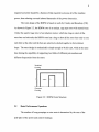
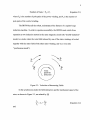


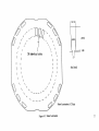
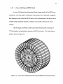


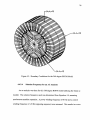


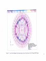

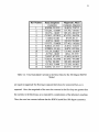
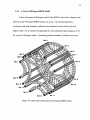
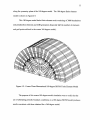
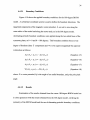
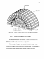

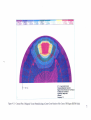

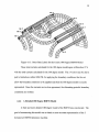
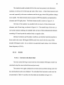
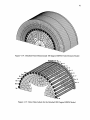


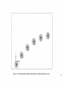
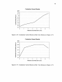
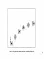
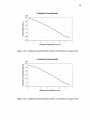


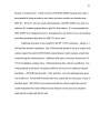


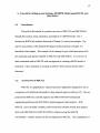


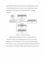

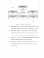


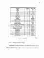


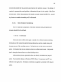


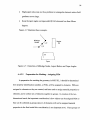
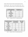


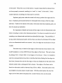


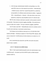

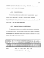


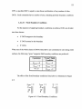


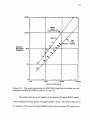


![[U2.10.02] Notice d`utilisation de MFront avec Code_Aster](http://vs1.manualzilla.com/store/data/006367052_1-f039eaa7ebc9872f5b28ed86f18edd22-150x150.png)